Diffusion Models in Low-Level Vision: A Survey

Abstract

Deep generative models have garnered significant attention in the realm of low-level vision tasks due to their formidable generative capabilities. Among them, diffusion model-based solutions, characterized by their utilization of a forward diffusion process for destroying an image and a reverse denoising process for image generation, have emerged as widely acclaimed for their ability to produce samples of superior quality and diversity. This ensures the generation of visually compelling results with intricate texture information. Despite their remarkable success and widespread application in low-level vision, a noticeable gap exists in the form of a comprehensive and illuminating survey that amalgamates these pioneering diffusion model-based works and organizes the corresponding threads. To address this void, this paper proposes the inaugural comprehensive review centered on denoising diffusion model-based techniques applied in low-level vision tasks, encompassing both theoretical and practical contributions to the field. We present three generic diffusion modeling frameworks and explore their correlations with other commonly used deep generative models, thereby establishing the theoretical foundation for subsequent analyses. Following this, we introduce a multi-perspective categorization of diffusion models employed in low-level vision tasks, considering both the underlying framework and the target task. Additionally, beyond natural image processing methods, we summarize extended diffusion models applied in other low-level vision tasks, including medical, remote sensing, and video scenarios. Moreover, we provide an overview of commonly used benchmarks and evaluation metrics in low-level vision tasks. We conduct a thorough evaluation, encompassing both performance and efficiency, of diffusion model-based techniques in three prominent tasks. Finally, we elucidate the limitations of current diffusion models and propose seven intriguing directions for future research. This comprehensive examination aims to facilitate a profound understanding of the landscape surrounding denoising diffusion models in the context of low-level vision tasks. For those interested, a curated list of diffusion model-based techniques, datasets, and other related information in over 20 low-level vision tasks can be found at https://github.com/ChunmingHe/awesome-diffusion-models-in-low-level-vision.

1 Introduction

Serving as an essential part of computer vision, low-level vision tasks have been extensively explored for enhancing the low-quality data degraded by complex scenarios and thereby encompass wide and practical applications, including but not limited to image super-resolution [1], deblurring [2], dehazing [3], inpainting [4], fusion [5], compression sensing[6], low-light enhancement [7], and remote sensing cloud removal [8]. See Fig. 1 for visual results.

(a) Image Super-resolution

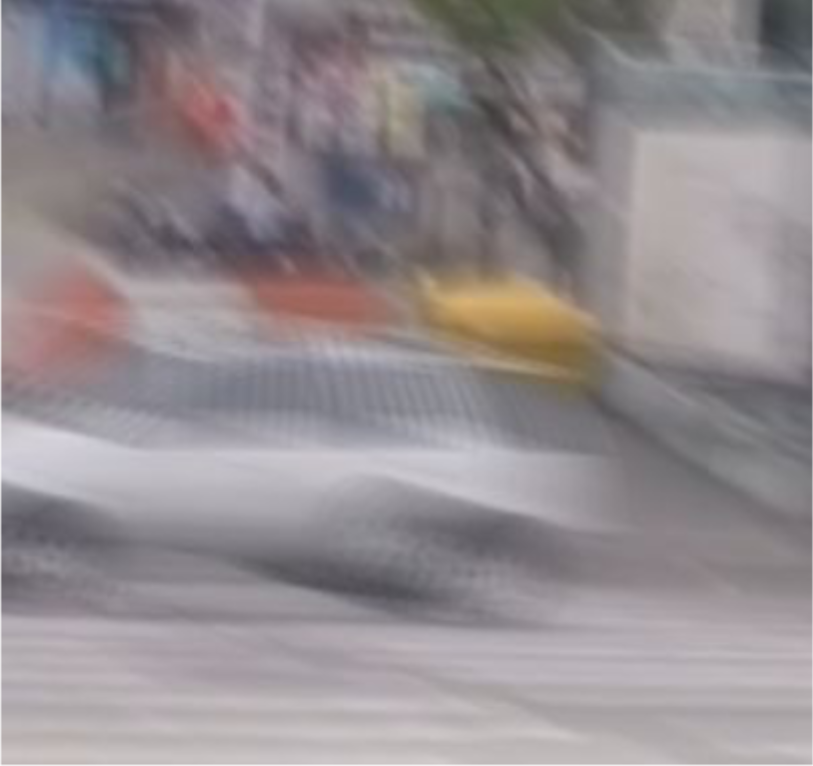
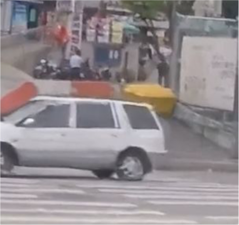
(b) Image Deblurring

(c) Image Inpainting

(d) Low-light Image Enhancement

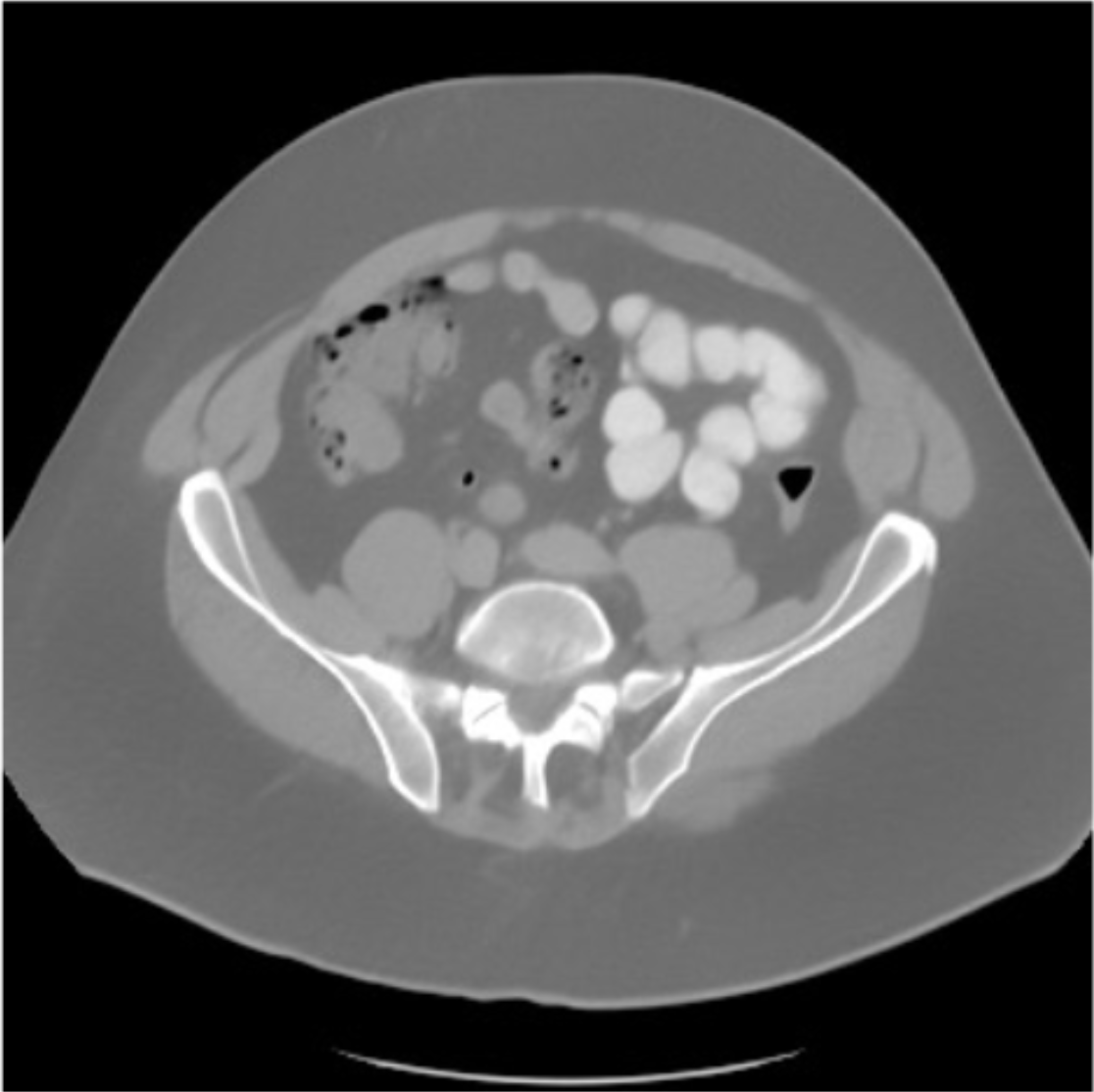
(e) Limited-angle CT Reconstruction

(f) Cloud Removal

Figure 1: Examples of various low-level vision tasks with the low-quality image (left) and the enhanced high-quality image (right). Notice that all the enhanced results are generated with diffusion model-based algorithms, which are IDM [9] in (a), MSGD [10] in (b), Repaint [11] in (c), Reti-Diff [7] in (d), DOLCE [12] in (e), and DDPM-CR [8] in (f).

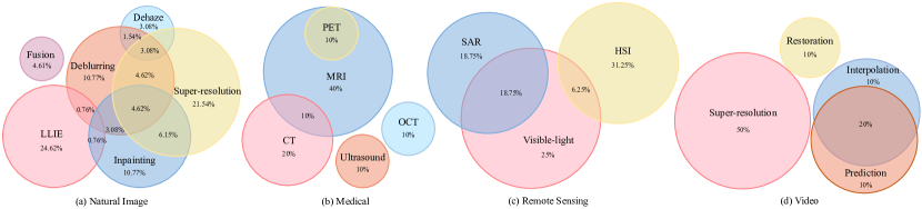
Figure 2: Distributions of the four main low-level vision scenarios of DM-based models. In each Venn diagram, the overlapping regions between circles indicate that these models are capable of addressing multiple application tasks or input modalities.

Traditional approaches [13, 14] formulated the problem as a variational optimization challenge and employed handcrafted algorithms to solve the proximity constraints related to certain image properties or degradation priors [15, 16]. Those methods, however, fail to cope with the complex degradation for lacking generalizability. With the advent of deep learning, convolutional neural networks (CNNs) [17] and transformers [18] are widely used in low-level vision tasks for their powerful feature extraction capacities. Besides, the collection of abundant datasets, e.g., DIV2K [19] in super-resolution and Rain800 [20] in deraining, further promotes their generalizability. Although achieving promising results, especially in distortion-based metrics like PSNR and SSIM, those techniques suffer from unsatisfactory texture generation, limiting the application in real-world scenarios.

In response to this limitation, deep generative models, especially generative adversarial networks (GANs) [21], have been introduced to the field of low-level vision. Benefiting from their powerful generative capacities, these networks are expected to synthesize realistic texture details and thus can be extended to real-world scenarios. However, those strategies still encounter several critical challenges: (1) The training process is susceptible to mode corruption and unstable optimization, necessitating intricate hyperparameter tuning during training. (2) The generated results can still exhibit artifacts and counterfactual details, undermining global coherence and limiting their applicability range.

A novel deep generative model, termed diffusion models (DMs) [22, 23, 24, 25, 26, 27, 28, 29, 30], has recently emerged as a hot topic in computer vision for its remarkable generative capacities and training stability. DMs, characterized by a forward diffusion stage and a reverse diffusion stage, systematically perturb data by introducing noise and subsequently learn to reverse this process for sample generation. Operating within the category of likelihood-based models, DMs formulate their training objective as a re-weighted variational lower bound, garnering acclaim for their extensive distribution coverage, stationary training objective, and straightforward scalability.

Leveraging the above advantages, DMs have exhibited significant success across multiple domains, encompassing data generation, image content comprehension, and low-level vision. Within the realm of low-level vision, DMs [9, 10, 31, 32] mainly concentrate on the restoration of low-quality data, ensuring the reconstruction of high-quality data with precise semantic information and realistic texture details, even in real-world scenarios characterized by complex and severe degradation. As depicted in Fig. 1, numerous DM-based algorithms have demonstrated promising outcomes across various low-level vision tasks. However, the techniques employed in different tasks exhibit considerable diversity and complexity, rendering them challenging to comprehend and enhance, thereby posing obstacles to future development and the introduction of a general-purpose reconstruction model. In light of this, there is a pressing need for a well-structured and comprehensive DM-based survey within low-level vision tasks. Nonetheless, most existing DM-based surveys [33, 34, 35, 36] focus on foundational theoretical models and the development of those generation-based techniques. Only a few surveys [37, 38, 39] concentrate on one specific problem or a few limited tasks within natural image scenarios in low-level vision tasks.

To address the needs of the field and mitigate the above drawbacks, we propose the first DM-based survey tailored for low-level vision tasks (see Figs. 2 and 3). This survey comprises a detailed theoretical introduction, wide application scopes, thorough experimental analysis, and extensive future perspectives. In specific, we commence with a comprehensive introduction to the fundamentals of diffusion models in Sec. 2, elucidating the connections and interrelations between DMs and other deep generative models. Then, we summarize existing cutting-edge DM-based natural low-level vision methods in Sec. 3, categorizing them based on the underlying framework and the target task, including six widely-used tasks. We then expand our scope in Sec. 4 to encompass broader scenarios, including medical, remote sensing, and video scenarios, aiming to provide a comprehensive overview with wide application ranges. Furthermore, Sec. 5 compiles collections of over 30 commonly used benchmarks and more than 10 fundamental evaluation metrics in low-level vision tasks. Abundant experiments on DM-based methods across three prominent tasks, including super-resolution, image deblurring, and low-light image enhancement, are provided in their corresponding settings. Finally, we identify the limitations of existing DM-based methods in low-level vision tasks and propose three main potential directions for future research and improvements in Sec. 6, and summarize the survey in Sec. 7.

Figure 3: The bar chart illustrates the continuous growth of diffusion model-based methods in low-level vision tasks across four distinct scenarios. Representative works from various periods are categorized and marked on the line graph with colors corresponding to each scenario as indicated in the legend. The methods highlighted in the figure represent the seminal works of each period, e.g., StableSR [40] has garnered 1.9k GitHub stars, while SR3 [41] boasts 1.2k citations.

We aspire that this DM-based survey, aimed at advancing the understanding of the low-level vision field, will inspire further interest in the computer vision community and promote related research endeavors.

Note. In formulating our search strategy, we executed a comprehensive exploration across diverse databases, including DBLP, Google Scholar, and ArXiv Sanity Preserver. Our emphasis was particularly placed on reputable sources, such as TPAMI, IJCV, and TIP, as well as esteemed conferences like CVPR, ICCV, and ECCV. Preference was accorded to studies that furnished official codes, thereby augmenting reproducibility, as well as those garnering higher citations and Github stars, indicative of broader acknowledgment and adoption within the academic community. Subsequent to this initial screening, our literature selection process entailed a meticulous evaluation of each paper’s novelty, contribution, and significance, along with assessing whether it constituted seminal work in the field. While acknowledging the potential omission of noteworthy papers, our endeavor was to present a comprehensive overview of the most influential and impactful research, thereby fostering research advancement and suggesting potential future avenues.

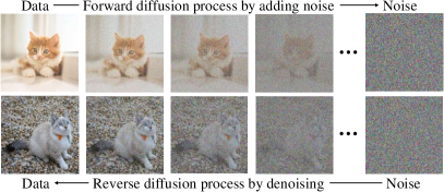
Figure 4: The schematic diagram of diffusion models.

2 A Walk-through of diffusion models

Diffusion models constitute a category of likelihood-based models. They are characterized by a shared principle of progressively perturbing data through a random noise process known as “diffusion” and then removing the noise to produce samples (see Fig. 4). These models are typically classified into three subcategories: denoising diffusion probabilistic models (DDPMs), noise-conditional score networks (NCSNs), and stochastic differential equations (SDEs).

DDPMs and their variants have garnered significant attention owing to their straightforward algorithmic flow and the ease of integrating conditional controls. In contrast, NCSNs and SDEs are often subject to detailed mathematical analysis, given their potential for more efficient sampling and enhancements in task generalization. In the following subsections, we will delve into these three formulations, elucidating the noise introduction and reversal process, and outlining the generation of new samples during inference.

2.1 Denoising Diffusion Probabilistic Models

A vanilla DDPM employs two Markov chains: a forward chain that perturbs data into random noise, and a reverse chain that converts the noise back to data. The initial diffusion process transforms data ${{x}_{0}}\sim q({{x}_{0}})$ from a complex distribution into a latent variable ${{x}_{T}}$ in a fixed simple prior distribution (e.g., standard Gaussian) over $T$ timesteps. At each diffusion step, Gaussian noise $\varepsilon$ is added to the data, following a hand-designed variance schedule $\{{{\beta}_{1}},\ldots,{{\beta}_{T}}\}$, and ${{x}_{t}}\in{{\mathbb{R}}^{d}}$, $t\in\{1,2,\ldots,T\}$, sharing the same dimension $d$ as ${{x}_{0}}$. Hence, the forward process can be expressed as the posterior $q({{x}_{1}},\ldots,{{x}_{T}}|{{x}_{0}})$ based on the Markov chains:

$$q({{x}_{1}},\cdots,{{x}_{T}}|{{x}_{0}}):=\mathchoice{\mathop{\vbox{\hbox{\scalebox{0.8}{$\displaystyle\prod$}}}}}{\mathop{\vbox{\hbox{\scalebox{0.8}{$\textstyle\prod$}}}}}{\mathop{\vbox{\hbox{\scalebox{0.8}{$\scriptstyle\prod$}}}}}{\mathop{\vbox{\hbox{\scalebox{0.8}{$\scriptscriptstyle\prod$}}}}}_{t=1}^{T}{q({{x}_{t}}|{{x}_{t-1}})},$$ (1)

$$q({{x}_{t}}|{{x}_{t-1}}):=\mathcal{N}({{x}_{t}};\sqrt{1-{{\beta}_{t}}}{{x}_{t-1}},{{\beta}_{t}}\bf I),$$ (2)

given the hyperparameters ${\alpha}_{t}:=1-{{\beta}_{t}}$, $~{}{{\bar{\alpha}}_{t}}:=\mathchoice{\mathop{\vbox{\hbox{\scalebox{0.8}{$\displaystyle\prod$}}}}}{\mathop{\vbox{\hbox{\scalebox{0.8}{$\textstyle\prod$}}}}}{\mathop{\vbox{\hbox{\scalebox{0.8}{$\scriptstyle\prod$}}}}}{\mathop{\vbox{\hbox{\scalebox{0.8}{$\scriptscriptstyle\prod$}}}}}_{s=1}^{t}{{{\alpha}_{s}}}\text{ }$. The above equations can be reformulated as

$$q({{x}_{t}}|{{x}_{0}})=\mathcal{N}({{x}_{t}};\sqrt{{{{\bar{\alpha}}}_{t}}}{{x}_{0}},(1-{{\bar{\alpha}}_{t}})\bf I).$$ (3)

By reparameterizing Eq. 3, ${x}_{t}$ can be calculated as

$${{x}_{t}}({{x}_{0}},\epsilon)=\sqrt{{{{\bar{\alpha}}}_{t}}}{{x}_{0}}+\sqrt{1-{{{\bar{\alpha}}}_{t}}}\epsilon,\epsilon\sim\mathcal{N}(0,\bf I).$$ (4)

While the latter process ${{p}_{\theta}}({{x}_{0}})=\int{{{p}_{\theta}}({{x}_{0:T}})d{{x}_{1:T}}}$ reverses the former from $p({{x}_{T}})=\mathcal{N}({{x}_{T}};0,\bf I)$.

$${{p}_{\theta}}({{x}_{t-1}}|{{x}_{t}})=\mathcal{N}({{x}_{t-1}};{{\mu}_{\theta}}({{x}_{t}},t),{{\mathchoice{\mathop{\vbox{\hbox{\scalebox{0.6}{$\displaystyle\sum$}}}}}{\mathop{\vbox{\hbox{\scalebox{0.6}{$\textstyle\sum$}}}}}{\mathop{\vbox{\hbox{\scalebox{0.6}{$\scriptstyle\sum$}}}}}{\mathop{\vbox{\hbox{\scalebox{0.6}{$\scriptscriptstyle\sum$}}}}}}_{\theta}}({{x}_{t}},t)),$$ (5)

where learnable Gaussian transitions kernels with $\theta$ are parameterized by deep neural networks under the training objects of minimizing the Kullback-Leibler (KL) divergence between $q({x_{0}},{{x}_{1}},\cdot\cdot\cdot,{{x}_{T}})$ and ${{p}_{\theta}}({{x}_{0}},{{x}_{1}},\cdot\cdot\cdot,{{x}_{T}})$.

The optimization principle is as follows: To generate $x_{0}$ in the reverse process, we sample from the noise vector $x_{T}\sim p(x_{T})$ to obtain $x_{T-1},x_{T-2},\ldots,x_{1},x_{0}$ using the learnable transition kernel. The key to this sampling process is training the reverse Markov chain to match the actual time reversal of the forward Markov chain. This requires adjusting $\theta$ to align the joint distribution of the reverse Markov chain $p_{\theta}(x_{0},x_{1},\ldots,x_{T})$ closely with that of the forward process $q(x_{0},x_{1},\ldots,x_{T})$. We use the KL divergence to characterize the gap between these two distributions. $\theta$ can be trained by minimizing the KL divergence:

$$\begin{split}&KL(q({{x}_{0}},{{x}_{1}},\cdot\cdot\cdot,{{x}_{T}})||{{p}_{\theta}}({{x}_{0}},{{x}_{1}},\cdot\cdot\cdot,{{x}_{T}}))\\ &\overset{(i)}{\mathop{=}}\,-{{\mathbb{E}}_{q({{x}_{0}},{{x}_{1}},\cdot\cdot\cdot,{{x}_{T}})}}[\log{{p}_{\theta}}({{x}_{0}},{{x}_{1}},\cdot\cdot\cdot,{{x}_{T}})]+const\\ &\overset{(ii)}{\mathop{=}}\,-{{\mathbb{E}}_{q({{x}_{0}},{{x}_{1}},\cdot\cdot\cdot,{{x}_{T}})}}[-\log p({{x}_{T}})-\sum\limits_{t=1}^{T}{\frac{{{p}_{\theta}}({{x}_{t-1}}|{{x}_{t}})}{q({{x}_{t}}|{{x}_{t-1}})}}]\\ &\geq\mathbb{E}[-\log{{p}_{\theta}}({{x}_{0}})]+const.\end{split}$$ (6)

For better sample quality, a simplified form of loss function is proposed as the optimization target of the model[42]:

$${{\mathbb{E}}_{t\sim\mathcal{U}\left[\!\left[1,T\right]\!\right],{{x}_{0}}\sim q({{x}_{0}}),\epsilon\sim\mathcal{N}(0,\bf I)}}\left[\lambda(t){{\left\|\epsilon-{{\epsilon}_{\theta}}({{x}_{t}},t)\right\|}^{2}}\right],$$ (7)

where $\lambda(t)$ is a positive weighting function computed from Eq. 4. $\mathcal{U}\left[\!\left[1,T\right]\!\right]$ represents a uniform distribution over the set $\{1,2,\ldots,T\}$. ${{\epsilon}_{\theta}}$ is a deep network with parameters $\theta$ that predicts the noise vector $\epsilon$ given ${{x}_{t}}$ and $t$.

2.2 Noise Conditioned Score Networks

Figure 5: The flowcharts of various generative models.

NCSNs are designed to estimate the probabilistic distribution of the target data from the score function, which guides the sampling process progressively toward the center of the data distribution. The score function for a specific data density $p(x)$ is defined as the gradient of the log-density function, ${{\nabla}{x}}\log p\left(x\right)$, which defines a vector field over the entire space that data $x$ inhabits, pointing towards the directions along which the probability density function has the largest growth rate. The directions provided by these gradients are utilized by the Langevin dynamics algorithm [23] to iteratively shift from a random prior sample ${{x}_{0}}$ to samples ${{x}_{T}}$ in regions with high density. By learning the score function of a real data distribution, it is possible to generate samples from any point in the same space by iteratively following the score function until a peak is reached. Specifically, the process can be represented as:

$${{x}_{t}}={{x}_{t-1}}+\frac{\gamma}{2}{{\nabla}_{x}}\log p(x)+\sqrt{\gamma}{{\epsilon}_{t}},$$ (8)

where $t\sim\mathcal{U}\left[\!\left[1,T\right]\!\right]$. $\gamma$ controls the updating magnitude in the direction of the score, akin to the learning rate in stochastic gradient descent. The noise ${{\epsilon}_{t}}\sim\mathcal{N}\left(0,\mathbf{I}\right)$ represents random normal Gaussian noise at time step $t$, introducing random perturbations into the recursive process to address the issue of getting stuck in local minima. As the time step $T\to\infty$ and $\gamma\to 0$, the distribution $p\left({{x}_{T}}\right)$ approaches the original data distribution $p(x)$. Hence, a generative model can utilize the above method to sample from $p(x)$ after estimating the score with a network ${{s}_{\theta}}\left(x,\text{ }t\right)\approx{{\nabla}_{x}}\log\text{ }{p}\left(x\right)$. This network can be trained via score matching [43] to optimize the objective function presented as follows:

$$\underset{\theta}{\mathop{\min}}\ {\mathbb{E}}_{t,{{x}_{0}},{x}_{t}}[\lambda(t)\|{{s}_{\theta}}({x}_{t},t)-{{\nabla}_{{{x}_{t}}}}\log p({x}_{t}|{x}_{0})\|_{2}^{2}],$$ (9)

where $t\sim\mathcal{U}\left[\!\left[1,T\right]\!\right],{{x}_{0}}\sim p({{x}_{0}}),{x}_{t}\sim{{p}}({x}_{t}|{x}_{0})$. In practice, because $\nabla_{x_{t}}\log p(x_{t}|x_{0})$ is unknown, Eq. 9 can only be solved by those score matching-based methods rather than be directly solved, limiting the generalization to real data. According to the manifold hypothesis, conventional score function estimation methods, including denoising score matching [43] and sliced score matching [44], when combined with Langevin dynamics, can lead the resulting distribution to collapse to a low-dimensional manifold and thus bring inaccurate score estimation in the low-density region. To address this issue, annealed Langevin dynamics perturbs the data with Gaussian noise at different scales and further proposes an optimization objective under a monotonically decreasing noise strategy $({{\sigma}_{t}})_{t=1}^{T}$:

$$\mathcal{L}\left(\theta,{{\sigma}_{t}}\right)\!=\!\frac{1}{T}\sum\limits_{t=1}^{T}{\lambda(}{{\sigma}_{t}}){{\mathbb{E}}_{p(x),{{x}_{t}}}}[\|{{s}_{\theta}}({{x}_{t}},{{\sigma}_{t}})\!+\!\frac{{{x}_{t}}-x}{\sigma_{t}^{2}}\|_{2}^{2}],$$ (10)

where ${{{{x}_{t}}\sim{{p}_{{{\sigma}_{t}}}}({{x}_{t}}\left|x)\right.}}$. In inference, one can initiate with white noise and apply Eq. 8 for a predetermined $T$. Once ${{\theta}^{*}}$ is acquired through optimizing the objective conditioned on $T$, as shown in Eq. 10, one can use the approximation ${{\nabla}_{x_{t}}}\log{p}\left({{x}_{t}}\right)\approx{{s}_{{{\theta}^{*}}}}\left({{x}_{t}},\text{ }t\right)$ as a plug-in estimate to replace the score function used in the stochastic differential equations [45]. As iterative processes continue, the final sample is derived from the output obtained at $t=0$.

2.3 Stochastic Differential Equations

As a continuous extension of NCSNs, SDE and reverse-time SDE can corresponding model the forward diffusion process and reverse diffusion process, respectively. The forward diffusion process modeled by SDE is formulated as

$$\frac{dx}{dt}=\bar{f}(x,t)+\bar{g}(t)\omega_{t}\Leftrightarrow\ dx=\bar{f}(x,t)dt+\bar{g}(t)d\omega,$$ (11)

where $\bar{f}(x,t)$ and $\bar{g}(t)$ are diffusion and drift functions of the SDE. ${\omega}\in{{\mathbb{R}}^{n}}$ denotes the standard n-dimensional Wiener process. Based on Eq. 11, the reverse process can be modeled with a reverse-time SDE [45], which is

$$dx=[\bar{f}(x,t)-\bar{g}{{(t)}^{2}}{{\nabla}_{x}}\log{{p}_{t}}(x)]dt+\bar{g}(t)d\bar{\omega},$$ (12)

where $d\bar{\omega}$ denotes the infinitesimal negative time step, defining the standard Wiener process running backward in time. Solutions to the reverse-time SDE are diffusion processes that gradually convert noise to data. Note that the reverse SDE defines the generative process through the score function ${{\nabla}_{x}}\log p(x)$, a shared concept in Sec. 2.2.

During both train and inference phases, SDE-based methods rely on practical numerical sampling techniques. Alongside numerical solutions discussed in Sec. 2.2, methodologies like Euler-Maruyama discretization and Ordinary Differential Equations (ODEs) [46] are effective, with the latter offering better sample efficiency advantages.

If the score function ${{\nabla}_{x}}\log p(x)$ is known, we can solve the reverse-time SDE easily. By generalizing the score-matching optimization objective in NCSNs to continuous time, we parameterize a time-dependent score model $s_{\theta}(x_{t},t)$ to estimate the score function in reverse-time SDE, bringing the same optimization objective as Eq. 9.

Comparing the expansion result of the score function that uses Bayes’ rule with the noise result obtained from Eq. 4, it is easy to observe that the training objectives for DDPMs and NCSNs are equivalent, as shown in Eq. 13. Namely, the optimization learning objectives of both methods only differ by a fixed scaling factor:

$${{s}_{\theta}}({{x}_{t}},t)=-\frac{1}{\sqrt{1-{{{\bar{\alpha}}}_{t}}}}{{\epsilon}_{\theta}}({{x}_{t}},t).$$ (13)

Moreover, when generalizing to the case of infinite time steps or noise levels, both DDPMs and NCSNs can be considered as discrete numerical solutions of SDEs in practical applications. For example, the Variance Preserving (VP) [30] form of the SDE can be perceived as the continuous version of DDPM [25], and the corresponding SDE is

$$dx=-\frac{1}{2}\beta(t)xdt+\sqrt{\beta(t)}d\omega,$$ (14)

where $\beta(\frac{t}{T})=T{{\beta}_{t}}$ as $T$ goes to infinity. NCSNs with annealed Langevin dynamics are equivalent to the discrete version of Variance Exploding (VE) SDE [30], which is

$$dx=\sqrt{\frac{d[\sigma{{(t)}^{2}}]}{dt}}d\omega,$$ (15)

where $\sigma(\frac{t}{T})={{\sigma}_{t}}$ as $T$ goes to infinity.

2.4 Comparisons With Other Deep Generative Models

In this subsection, we explore the connections between diffusion models and other commonly-used generative models, whose flowcharts are illustrated in Fig. 5.

Both DMs and variational autoencoders (VAEs) [47, 48] involve mapping data to a latent space, where the generative process learns to transform the latent representations back into data. Additionally, in both cases, the objective function can be derived as a lower bound of the data likelihood. However, while the latent representation in VAEs contains compressed information about the original image, classical assumptions suggest that DMs completely destroy the data after the final step of the forward process. Furthermore, the latent representations in diffusion models have the same dimensions as the original data, whereas VAEs tend to perform better with reduced dimensions. Drawing inspiration from these similarities, some existing work has explored the use of diffusion models on the latent space of a VAE to build more efficient models [26, 49, 50], or to construct hybrid models that fully leverage the advantages of both models.

Normalizing flows (NFs) [51, 52] transform a simple Gaussian distribution into a complex data distribution through a series of invertible functions with easily computable Jacobian determinants. The only similarity between DMs and NFs lies in their mapping of the data distribution to Gaussian noise. However, the learnable forward process of NFs, unlike that of DMs, imposes additional constraints on the architecture due to its requirement for invertible and differentiable properties. DiffFlow [53], serving as a bridge between these two generative algorithms, extends both diffusion models and normalizing flows to enable trainable stochastic forward and reverse processes.

GANs [54] drive the fake data distribution towards the real one through adversarial learning on the generator and the discriminator, ensuring that the sampled data resembles real data. Consequently, GANs are extensively utilized for generating photo-realistic high-resolution images (e.g., PGGAN [55] and StyleGAN series [56]). However, GANs are notorious for their challenging training process due to their adversarial objective [57] and often suffer from mode collapse. In contrast, DMs exhibit a stable training process and offer greater diversity as they are likelihood-based. Despite these advantages, DMs are less efficient than GANs as they require multiple iterative steps during inference.

The distinctions between GANs and DMs also manifest in their ability to manipulate semantic properties within the latent space. GANs’ latent space has been observed to contain subspaces associated with visual attributes, enabling attribute manipulation through changes in the latent space and thus facilitating more precise control over generated images. However, DMs manipulate semantic properties of the latent space in a more implicit and less controllable manner. Fortunately, Song et al. [28] demonstrate that DMs’ latent space exhibits a well-defined structure. Nonetheless, the exploration of DMs’ latent space has been less extensive compared to GANs, indicating the need for further research.

3 Diffusion models for natural image processing in low-level vision

To begin with, we first give the definition of ”natural images”, which depict common scenes and objects encountered in daily life, serving as the foundational input data in model training and evaluation, particularly for image restoration algorithms. In this section, ”images” encompass the ordinary and general notion of natural images.

Low-level vision tasks primarily focus on various ill-posed inverse problems in the image restoration domain. These tasks aim to restore degraded and noisy low-quality (LQ) images to high-quality (HQ) images. The general form of the forward model can be stated as

$$~{}y=H({{x}_{0}})+n,\text{ }\ \ y,n\in{{\mathbb{R}}^{n}},{x}_{0}\in{{\mathbb{R}}^{d}},$$ (16)

where $H(\cdot):{{\mathbb{R}}^{d}}\to{{\mathbb{R}}^{n}}$ is the forward measurement operator that maps the clean image ${x}_{0}$ to the distorted data $y$. In addition, $n$ is the measurement noise.

Through rapid development, DM-based models have achieved significant progress in this domain. Unlike random sample generation methods such as vanilla DDPM in Sec. 2, here the degraded LQ images are used as conditional inputs to guide the latent variables during inference. The models are expected to learn a parametric approximation to the unknown conditional distribution, posterior $p\left(x|y\right)$, through a stochastic iterative refinement process.

After conducting a comprehensive review of approximately 100 relevant DM-based works, we classify them from two perspectives. First, according to whether the DMs require training, we classify those methods into supervised and zero-shot DM-based methods. Additionally, we categorize them depending on the task being solved, e.g., super-resolution and low-light image enhancement.

3.1 DM-based methods with different training manners

DM-based models typically employ two training methods: supervised and zero-shot. Research has flourished in both paradigms, demonstrating the versatility of DMs as frameworks for various low-level vision tasks.

Supervised DM-based methods. Supervised DM-based methods tend to specialize in addressing specific degradation scenarios. They employ the well-designed conditional mechanism to incorporate distorted images as guidance during the reverse process, enabling them to tackle several extreme challenges, such as dehazing, deraining, and desnowing, that cannot be effectively modeled using the form of Eq. 16. However, despite yielding promising texture generation performance, these approaches require training the diffusion model from scratch using paired clean and distorted images from a particular degradation scenario. This results in costly data acquisition and limits the algorithm’s generalization to other degradation scenarios.

Figure 6: Linear and nonlinear inverse problems with DMs-based solutions. Figure adapted from [58].

Zero-shot DM-based methods. Zero-shot DM-based techniques, leveraging the image priors extracted from pre-trained diffusion models, offer an appealing alternative as they are plug-and-play without retraining on a specific dataset. The underlying concept is based on the understanding that pre-trained generative models, constructed using extensive real-world datasets such as ImageNet [59], can serve as a repository of structure and texture. A key challenge of zero-shot DM-based methods lies in extracting the corresponding perceptual priors while preserving the underlying data structure from distorted images. Consequently, these zero-shot DM methods are often applied to degradation scenarios simplified as linear reverse problems, such as super-resolution and inpainting. Given the simplicity of the application process, which only requires replacing the forward measurement operator, evaluating performance on linear inverse problems has become a common practice to assess the generalization of newly proposed conditional diffusion models. However, these works are frequently categorized under multi-task alongside other high-level tasks in existing surveys, without receiving systematic analysis and summarization. Therefore, we devote a specific subsection to introducing these DM-based inverse problem solvers for general-purpose image restoration in Sec. 3.2.

3.2 DM-based methods with different application goals

To provide a comprehensive overview, we categorize existing DM-based methods into the general-purpose image restoration task, encompassing most zero-shot methods and several supervised methods and six distinct specific tasks, including super-resolution (SR), inpainting, deblurring, dehazing, low-light image enhancement, and image fusion.

General-purpose image restoration. Notably, most methods in this subsection presuppose prior knowledge of the forward operator $H(\cdot)$ in Eq. 16, thereby confining their scope to non-blind inverse problems. To adhere to specific assumptions, further constraints are occasionally imposed to convert them into linear inverse problems, as shown in Fig. 6. Nonetheless, the mapping $y\to x_{0}$ remains many-to-one, rendering it impossible to precisely recover $x_{0}$.

Focusing on sampling from the posterior $p(x|y)$, the relationship can be formally established with the Bayes’ rule: $p(x|y)=p(y|x)p(x)/p(y)$. However, apart from $p(y|{{x}_{0}})\sim\mathcal{N}(y|A({{x}_{0}}),\text{ }{{\sigma}^{2}}\bf I)$, there does not exist explicit dependency between $y$ and ${{x}_{t}}$, where ${{x}_{t}}$ denotes the noisy results at time step $t$. To solve the intractability of the posterior distribution, Song et al. [28] propose conditional denoising estimator (CDiffE) ${{s}_{\theta}}\left(x,\text{ }y,\text{ }t\right)$. The condition $y$ is added to the input of the estimator to learn an approximation to the posterior score function ${{\nabla}_{{{x}_{t}}}}\text{log }p\left({{x}_{t}}|y\right)$ without altering the training object. Instead of direct learning, the conditional diffusive estimator [28] jointly diffuses $x$ and $y$ and then learns the posterior approximated from the joint distribution $p\left({{x}_{t}},\text{ }{{y}_{t}}\right)$ using denoising score matching. Batzolis et al.[60] rigorously prove the effect of the above two methods theoretically and analyze the errors caused by the imperfections.

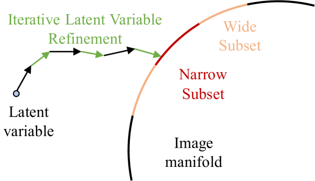
Figure 7: Guiding generation process in ILVR [61].

To enhance consistency, [62] and [61] guide the gradient towards high-density regions by conditioning it through projections on the measurement subspace without directly learning the posterior score function. Chung et al.[62] introduce the manifold constraint after the update step, which corrects deviations from the perfect data consistency. Utilizing pre-trained unconditional DDPM, Choi et al.[61] propose Iterative Latent Variable Refinement (ILVR). As shown in Fig. 7, ILVR is a learning-free method adopting low-frequency information from $y$ to guide the generation process towards a narrow data manifold. However, such approaches are limited to those noiseless inverse problems.

Besides the above learning-free methods, plug-and-play posterior sampling provides another favorable choice. According to the Bayesian framework, the posteriors are decomposed into likelihood functions and plug-and-play priors. The prior term is typically satisfied by generative diffusion models capable of learning robust assumptions about the underlying structure of images (e.g., the distribution of natural images), while the likelihood term, also known as the data term, is derived from the degradation model.

In plug-and-play sampling methods, Graikos et al.[63] first showcase the viability of directly using pre-trained DDPMs as plug-and-play modules that involve other differentiable constraints. Kawar et al.[64] propose the Denoising Diffusion Restoration Models (DDRM) to reconstruct the missing information in $y$ within the spectral space of $H(\cdot)$ using Singular Value Decomposition (SVD). Leveraging the power of pre-trained DMs, DDRM demonstrates versatility across several tasks, including SR, deblurring, inpainting, and colorization, even in the presence of varying levels of measurement noise. However, only linear inverse problems are viable in this framework due to the limitations of SVD.

Zhu et al.[65] decouple the data term and the prior term with Half-Quadratic-Splitting and propose DiffPIR, handling a wide range of degradation models with different degradation operators $H(\cdot)$, as the data term can be independently solved. Chung et al.[58] introduce a Laplacian approximation-based method named Diffusion Posterior Sampling for posterior sampling, applicable to nonlinear inverse problems with complex noise. Similarly utilizing DM as a prior term, Wang et al.[66] propose to solve zero-shot image restoration using Denoising Diffusion Null-space Model (DDNM). The pseudo-inverse based on SVD computes the low-dimensional image representation, then decomposed into its range and null-space components. By refining only the null-space during the reverse process, DDNM can learn missing information in image inverse problems while accommodating only linear operators.

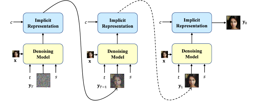
Figure 8: Outline of the IDM [9] framework.

Methods based on Schrödinger bridges, i.e., InDI[67] and I2SB[68], revisit DMs’ assumptions and depart from commencing the reverse diffusion process from Gaussian noise, ensuring efficiency. Chung et al.[69] demonstrate the equivalence of the above methods and propose the Consistent Direct Diffusion Bridge (CDDB), incorporating a previously overlooked data consistency module, to realize the generalization of Schrödinger bridges on low-level vision tasks. Similarly, Chung et al.[70] use a feed-forward network (FFN) to initialize the diffusion process and reduce sampling steps to generate images from pure noise, shedding light on combining existing FFNs for inverse problems with DMs.

To mitigate the computational overhead, researchers have shifted DMs from the image level to the vector level. Rombach et al.[26] propose latent diffusion models (LDMs), where both the forward and reverse processes occur in the latent space obtained through an auto-encoder. DiffIR[4] further compress latent variables to an extremely low-dimensional representation to guide the transformer in image reconstruction. To balance latent disentanglement and high-quality reconstructions, Pandey et al.[71] integrate VAEs within the diffusion model and propose DiffuseVAE, offering novel conditional parameterizations for DMs and providing a promising alternative for hybrid modeling.

Due to prevalent limitations stemming from various presuppositions, these models are frequently applied to relatively simple degradation scenarios that can be abstracted and simplified as linear inverse problems. Consequently, they are less effective in real-world blind tasks compared to task-specific methods.

Super-resolution (SR). Diffusion models have shown prowess in generating high-quality outputs with intricate details, addressing over-smoothing and artifacts commonly encountered for high-resolution SR[72, 73]. SRDiff[74] is the pioneering single-image SR model based on diffusion models, utilizing a pre-trained low-resolution encoder and a conditional noise predictor to produce diverse and realistic SR predictions. This approach effectively addresses over-smoothing and large footprint issues in previous methods[5]. Saharia et al.[75] also leverage a conditional diffusion network, employing low-resolution images as conditional inputs to resolve SR tasks, particularly for human faces.

Cascaded Diffusion Models (CDM) [76] propose to arrange multiple DMs sequentially. In specific, the initial model generates low-resolution images based on image classes while subsequent models progressively generate images with higher resolutions, facilitating SR at arbitrary magnifications but increasing training costs. Gao et al.[9] propose implicit DMs for continuous SR (in Fig. 8). They introduce a scale-adaptive conditioning mechanism to regulate resolution and adjust the ratio of realistic data and use implicit neural representation to capture complex structures across continuous resolutions. Niu et al. [77] first utilize a pre-trained SR model to generate high-resolution conditional inputs. Besides, they propose a $n^{th}$ order sampler to perform a deterministic denoising process, greatly reducing the iteration number. Wang et al. [40] propose StableSR to leverage prior knowledge encapsulated in pre-trained text-to-image DMs for blind SR. By utilizing a time-aware encoder, StableSR achieves promising restoration results without modifying the pre-trained synthesis model, preserving generative priors and minimizing training costs. Similarly leveraging generative diffusion priors, Lin et al. [78] design DiffBIR for blind image SR, decoupling the restoration process into two stages. Sunet al. [79] propose CoSeR, which leverages generative reference images from a pretrained LDM as implicit priors. It combines these generated results with low-resolution image priors and CLIP’s semantic priors as conditions to control the diffusion process, achieving cognitive SR. AlHalawani et al. [80] introduce DMs into the surveillance domain, verifying the superiority in license plate SR. Meanwhile, Wang et al. [81] propose the two-stage DR2 focusing on facial data, achieving desirable results.

Figure 9: Overview of RePaint [82].

Figure 10: Overview of the method proposed in [83].

Inpainting. As a probabilistic generative model, diffusion models exhibit robust generalization across different masks and effectively handle large missing regions while producing visually plausible results. RePaint [11] employs an enhanced denoising strategy involving resampling iterations to better condition images in Fig. 9. The model first uses a deep network to generate a rough estimate, which is then refined by a diffusion model with a Markov random field. To specify a desired inpainted object, Gebre et al. [84] input an extra target image to guide the generation of the masked region, providing valuable exploration in the controllable generation. Zhang et al. [85] employ both image and text as multimodal guidance. By integrating the inverse diffusion process with CLIP, semantic reference information is better encoded, thus enhancing performance and controllability.

Spatial diffusion model [86] employs a Markov random field and a network to estimate the missing pixels, which considers surrounding contexts and thus inpaints large missing regions. Saharial et al.[87] introduce Palette to explore diverse optimization objectives and underscore the significance of self-attention. BrushNet [88] is a plug-and-play model engineered to embed pixel-level masked features into any pre-trained DMs by separating masked image features and noisy latent into separate branches. Grechka et al. [89] propose a training-free DM-based method GradPaint for gradient-guided inpainting. GradPaint aims to improve the coherence and realism of generated images by using custom loss and gradient guidance, demonstrating promising results when generalized to various datasets.

Deblurring. Because realistic blur is often complex and non-uniform, modeling specific degradation prior can result in poor performance. Consequently, DMs in these domains often rely on hand-designed networks. Wang et al.[83] is the first to introduce diffusion models (as illustrated in Fig. 10) into the deblurring task, proposing a “predict-and-refine” conditional diffusion model. This model architecture comprises a deterministic data-adaptive predictor and a stochastic sampler, which refines the output through residual modeling. Ren et al.[10] introduce multiscale structure guidance in image-conditioned DPMs (icDPMs) for deblurring. Their guidance module projects the input image into a multiscale representation, where auxiliary priors provide information about edges. This guidance is integrated into the network’s intermediate layers as an implicit bias, enhancing the robustness by informing the coarse structure of the sharp image. Hierarchical Integration Diffusion Model (HI-Diff) in [90] leverages the diffusion model in a compact latent space to generate priors and fuse these priors into the regression-based model through a cross-attention mechanism, enabling generalization in complex blurry scenarios.

Laroche et al. [91] propose a DM-based blind image deblurring method. This method integrates DMs with the Expectation-Minimization (EM) estimation to jointly estimate restored images and the unknown blur kernel. Spetlik et al. [92] propose a DDPM-based method, SI-DDPM-FMO, for single-image object deblurring and trajectory recovery of fast-moving objects, getting competitive results to multi-frame methods. DiffEvent [93] firstly introduces DMs into the event deblurring task and designs diffusion priors for the image and the residual. To better adapt to real-world scenes, DiffEvent builds an Event-Blur Residual Degradation (EBRD) to provide pseudo-inverse guidance, enhancing subtle details and handling unknown degradation. Luo et al.[82] deviate from classical SDE and propose a novel approach called Image Restoration Stochastic Differential Equation (IR-SDE). The core is a mean-reverting SDE with a maximum likelihood objective for training. This ensures that the entire SDE will diffuse towards the mean $\mu$, representing the low-quality images with specific Gaussian noise, thus directly simulating the degradation process [94].

Figure 11: Framework of WeatherDiffusion [31].

Dehazing, deraining, and desnowing. Unlike linear inverse problems such as super-resolution and inpainting, real-world degradations like dehazing and deraining are complex and cannot be effectively modeled by a prior operator $H(\cdot)$. Consequently, they pose challenges for incorporation into general-purpose image restoration frameworks.

Özdenizci et al. [31] present a patch-based image restoration algorithm based on DDPMs called WeatherDiffusion (illustrated in Fig. 11). This approach facilitates size-agnostic image restoration by employing a guided denoising process with smoothed noise estimates across overlapping patches during inference, effectively mitigating the drawbacks of merging artifacts from independently restored intermediate results. WeatherDiffusion achieves superior performance on both weather-specific and multi-weather image restoration tasks, including dehazing, desnowing, deraining, and raindrop removal. Building upon the IR-SDE as the base diffusion framework, Luo et al. [32] further enhance it to perform restoration in a low-resolution latent space, which constitutes a resolution-agnostic architecture. This enhancement offers another viable option for handling large-size images. Additionally, they propose a latent-replacing pretraining strategy to improve training stability. Wang et al. [95] propose a Frequency Compensation block (FCB), equipped with a bank of filters that collectively amplify the mid-to-high frequencies of an input signal, aiming to enhance the reconstruction of image details in dehazing tasks and improve generalization to real haze scenarios.

Figure 12: Overview of the PyDiff [96].

Low-light image enhancement. Due to the intrinsic relationship between low-light image enhancement (LLIE) and the human visual perception of light intensity, various interpretive prior models have emerged, inspiring multiple approaches for integrating the advantages of physical models and generative networks. Consequently, compared to the relatively monolithic black-box design in other tasks, a plethora of research related to DMs has emerged in LLIE.

Zhu et al. [97] are pioneers in introducing DMs into LLIE within space-based visible cameras. This method effectively reduces computational complexity by diffusing processes on grayscale images and supplementing features with RGB images. Wu et al. [98] focus on restoring pure black images, providing a robust generative network for enhancing low-light images with diverse outputs. DiD [99], designed for downstream low-light text recognition, utilizes a bootstrap diffusion model to learn the distribution of light-enhancement curve parameters, preserving high-frequency details in dark conditions and alleviating the computational burden. Panagiotou et al. [100] employ DMs as a postprocessing technique, estimating the amount of noise present in an enhanced image in one pass through the model. Zhou et al. [96] propose the Pyramid Diffusion model named PyDiff (illustrated in Fig. 12) for LLIE, which progressively increases the resolution during the reverse process, effectively reducing computational burden. Jiang et al. [101] introduce a wavelet-based conditional diffusion model (WCDM), which leverages wavelet transform to reduce computation. Moreover, a high-frequency restoration branch module is proposed to supplement the diagonal information with vertical and horizontal details. Wang et al. [102] integrate DMs with a physics-based exposure model in the raw image space, where the reverse process can directly start from a noisy image instead of pure noise, boasting a small parameter size and fast inference speed. Lv et al. [103] input low-light images into a latent space for the diffusion process, also effectively reducing computation.

Some methods that integrate DMs with other advanced techniques have yielded superior results. LLDiffusion [104] proposes a degradation-aware learning scheme to integrate degradation representations from pre-trained models and proposes a dynamic diffusion module that considers both color maps and degradation. Hou et al. [105] regularize the ODE-trajectory and introduce a global structure-aware regularization term to constrain the intrinsic structures, along with an uncertainty-guided regularization to relax constraints on extreme situations. Diff-Retinex[106] decomposes the image into illumination and reflectance maps based on the Retinex theory and then uses multi-path DMs to estimate the light distribution and restore degradation. Adopting the opposite strategy, He et al. [7] propose a Retinex-based LDM to extract reflectance and illumination priors, and then perform decomposition and enhancement using a Retinex-guided transformer, ultimately achieving superior results. Yin et al. [107] achieve an interactive and controllable LLIE model based on a conditional DM. Users can customize the brightness level and enhance specific target regions with the assistance of the Segment Anything Model (SAM). To fully utilize the CLIP-based model prior, Xue et al. [108] introduce multimodal visual-language information and propose a novel approach named CLIP-Fourier Guided Wavelet Diffusion (CFWD). CFWD combines the strengths of wavelet transform, Fourier transform, and CLIP to guide the DM-based enhancement process in a multiscale visual-language manner, demonstrating the immense potential of integrating semantic features from CLIP and high-frequency detail recovery from the Fourier transform.

Figure 13: The overall framework of Dif-Fusion [109].

Image fusion. Image fusion is an often overlooked low-level vision task among researchers. However, its significance lies in its capacity to amalgamate complementary data from multiple images, elevating the overall visual quality and facilitating diverse downstream applications. Yue et al. [109] propose the first DM-based method for image fusion named Dif-Fusion (see in Fig. 13) to enhance color fidelity in infrared and visible image fusion. By creating a multi-channel data distribution using a denoising network, Dif-Fusion facilitates multi-source information aggregation and maintains high-quality color representation. The forward and reverse diffusion processes in the latent space enable the extraction of diffusion features for effective fusion, leading to superior results compared to existing methods.

Zhao et al.[110] propose DDFM for Multi-Modality Image Fusion. The conditional generation problem is divided into an unconditional DDPM for utilizing image generation priors and a maximum likelihood sub-problem for preserving cross-modal information of source images. The authors innovatively model the latter using a hierarchical Bayesian approach and integrate its EM algorithm-based solution into the unconditional DDPM, ensuring the generation of visually fidelity results. Cao et al.[111] propose the utilization of diffusion models for general image fusion tasks and devise two conditional injection modulation modules to introduce coarse-grained style information and fine-grained frequency information into the diffusion UNet. This method achieves state-of-the-art results with strong generalization performance, showcasing the potential of diffusion models in image fusion tasks. Li et al. [112] apply the DDPM model to the multi-focus image fusion task, showcasing the excellent performance and robustness of DM-based methods in terms of noise resistance and few-shot capabilities.

Figure 14: Overview of the method in[113].

4 Extended diffusion models

Beyond natural image processing scenarios, certain specialized domains—such as medical imaging, remote sensing, and video analysis—exhibit unique characteristics that necessitate the development of specifically tailored DM-based methods to address their distinct requirements.

4.1 Diffusion models for medical image processing

Compared with natural data, medical data acquisition typically involves more intricate and precise physical imaging processes [114, 115, 116], resulting in poor image quality due to equipment limitations and usage conditions (e.g., hospital throughput requirements, patient examination time constraints, and radiation dosage limits). Leveraging the robust learning capacity of DMs, researchers suggest that these models can implicitly capture knowledge related to imaging physics from dataset distributions. Hence, DM-based reconstruction methods have been introduced to address low-quality medical images degraded by imaging limitations, including limited-angle computed tomography (CT) and accelerated magnetic resonance imaging (MRI).

In addition to enhancing low-quality data, another significant application of DM-based algorithms is the generation of missing modalities. In disease diagnosis, the combination of multimodal data assists doctors in making more accurate diagnoses. However, the types of actual modal data collected are often limited, and aligning the acquired multimodal data can be challenging. DM-based image translation methods offer a potential solution in this regard. Furthermore, certain rarer medical images (e.g., Positron Emission Computed Tomography (PET) and Optical Coherence Tomography (OCT)) unavoidably contain speckle noise that traditional methods struggle to eliminate. Due to the nature of generative models in detail reconstruction, diffusion models are well-suited for addressing such issues.

To provide a multi-perspective categorization, we will classify methods according to their imaging modalities, covering MRI, CT, multi-modal, and other modalities.

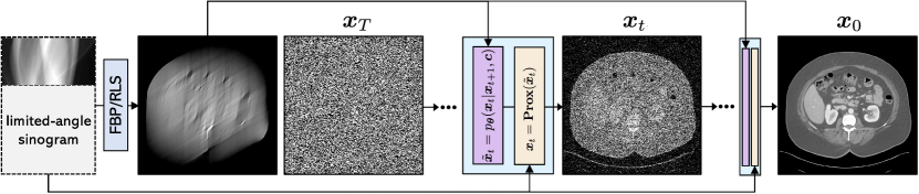
Figure 15: Overview of the proposed approach in[12].

Magnetic resonance imaging. Due to its inherent physics, MRI involves a time-consuming imaging process, where patient movement leads to various artifacts in the images. Hence, medical image reconstruction is necessary to achieve faster acquisition speed and solve this ill-posed inversion problem. Jalal et al.[117] initiate the primary study in MRI reconstruction using Compressed Sensing with Generative Models (CSGM). CSGM involves training score-based generative models on MRI images to provide prior information for inverting under-sampled MRI into realistic data through Langevin dynamics in a posterior sampling scheme.

Chung et al.[113] design a score-based framework for accelerated MRI reconstruction, illustrated in Fig. 14. Initially, they train a time-dependent score function using denoising score matching on magnitude images. They employ the VE SDE for sampling from the pre-trained score model distribution conditioned on the measurement. The reconstruction process involves splitting the image into real and imaginary components and applying data consistency mapping. Iterative steps include image division, correction, and further data consistency mapping for enhancement. It effectively handles multi-coil images and exhibits robust generalization, unaffected by subsampling patterns, unlike traditional models requiring retraining for each new sampling scheme.

CT. Similar to MRI, limited-angle CT reconstruction has been a primary focus in CT research, aiming to reduce patient radiation exposure and enhance examination throughput. DM-based methods have shown remarkable performance in this reconstruction task. For example, Liu et al. [12] introduce DOLCE, a method specifically designed for limited-angle CT reconstruction within a DDPM framework. Conventionally, the Filtered Back Projection (FBP) algorithm [118] is employed to map CT images from sinograms, leveraging the Fourier slice theorem. However, limited-angle measurements lead to Fourier measurement loss and subsequently degraded reconstruction outcomes.

Due to the ill-posed nature, directly using DDPM presents challenges. Following the design in inpainting tasks, DOLCE [12] integrates the FBP output on limited sinograms as prior information to condition the diffusion model (Fig. 15). Additionally, DOLCE enforces a consistency term in the denoising iteration to ensure reconstruction consistency through iterative refinement using proximal mapping in the inference step to meet the consistency conditions presented by sinograms. Evaluation on C4KC-KiTS verifies DOLCE’s effectiveness in generating high-quality CT images. Moreover, the reconstruction performance is further evaluated in downstream tasks such as 3D Segmentation.

Multi-modal medical data. MRI and CT are the two most widely used medical imaging modalities. MRI shows soft tissues such as vessels and organs in rich contrast while CT is preferred for imaging hard tissues such as bones and interfaces. Due to their complementary characteristics, multi-modality imaging with MRI and CT is often used in clinical practice. Therefore, the development of a simultaneous CT-MRI device is currently a hot research topic, and various studies have been carried out to propose advanced designs for such a device[119, 120, 121]. To translate MR to CT images, Lyu et al.[122] examine conditional DDPM and SDE models, employing three different sampling methods.

As shown in Fig. 16, Meng et al.[123] introduce a Unified Multi-Modal Conditional Score-based Generative Model (UMM-CSGM) to complete a wider range of missing modality images. This model is presented in a conditional format of SDE, leveraging a novel multi-in multi-out conditional score network (mm-CSN) module, to learn cross-modal conditional distributions. Experiments on BraTS19  [124] indicate that the method can generate missing-modality images with high fidelity and clear brain structural information.

Figure 16: Schematics of UMM-CSGM [123]. The upper panel shows the cross-modal diffusion and reverse generation process. The lower panel shows the structure of mm-CSN.

Due to the inter-modality differences and lacking medical data, training powerful DM-based models in a zero-shot manner for image translation is not feasible. However, this approach remains viable for translation tasks with lower difficulties, such as the CBCT-to-CT image translation and cross-institutional MRI image translation tasks. For example, Li et al. [125] propose the Frequency-Guided Diffusion Model (FGDM), which uses frequency-domain filters to preserve structure during image translation. FGDM enables zero-shot learning and exclusive training on target domain data, allowing direct deployment for source-to-target domain translation. This verifies significant advantages in zero-shot medical image translation over existing methods.

Other modalities. PET, crucial for cancer screening, faces challenges related to low SNR and resolution due to the limited beam count radiation during scans. To mitigate the oversmoothing in previous PET denoising methods, Gong et al. [126] introduce a DDPM-based framework for PET denoising, termed PET-DDPM. PET-DDPM explores the collaboration of diverse modalities to learn noise distribution through PET images. The MR image, serving as the prior, is seamlessly integrated as the input for the denoising network. Experiments reveal that employing MR prior as the input while embedding PET images as a data-consistency constraint during inference achieves the best performance.

Figure 17: General pipeline of DenoOCT-DDPM [127].

Hu et al.[127] apply a DDPM[25] to address speckle noise in OCT volumetric retina data using an unsupervised technique called DenoOCT-DDPM. OCT imaging encounters challenges due to restricted spatial-frequency bandwidth, resulting in images with speckle noise that hampers ophthalmologist diagnosis and tissue visibility, and conventional methods like averaging multiple B-scans struggle to handle this. DenoOCT-DDPM exploits DDPM’s adaptability to noise patterns instead of real-data patterns. It incorporates self-fusion[128] as a preprocessing step, feeding the DDPM with a clear reference image for training the parameterized Markov chain (refer to Fig. 17). The qualitative results support the efficacy of DMs in eliminating speckle noise while preserving detailed features like small vessels.

4.2 Diffusion models for remote sensing data

The versatility of diffusion models makes them well-suited for remote sensing data processing. Their applications span a spectrum of challenges encountered in the analysis of diverse remote sensing modalities, including visible-light images, hyperspectral imaging (HSI), and Synthetic Aperture Radar (SAR). These tasks encompass but are not limited to super-resolution [129, 130, 131], despeckling[132, 133], cloud removal[134, 8, 135], multi-modal fusion[111], and cross-modal image translation[136].

We continue to categorize these works based on the imaging modality, examining the significant impact and advancements brought about by diffusion models.

Visible-light remote sensing data. Compared with natural images, DM-based methods in remote sensing remain underdeveloped. Visible-light Remote Sensing Images share a high similarity with natural images. In this case, Sebaq et al.[137] employ techniques similar to Imagen [138] for low-resolution result generation and referenced the cascaded SR pipeline of CDM [76], ultimately constructing a powerful framework for high-resolution satellite imagery generation.

Given that RS images suffer from detail loss, Liu et al.[131] propose the first DM for Remote Sensing Super-Resolution (RSSR) and introduce a detailed supplement inpainting task through random masking, aiming to enhance the recovery ability for specific small objects and complex scenes. Besides, they introduce a joint loss to suppress the undesirable excessive diversity. Considering that RS images often have higher resolution and exhibit unusual sizes, Huang et al.[139] introduce an Adaptive Region-Based DM (in Fig. 18) capable of addressing arbitrary RS image dehazing tasks. They employ the cyclic shift strategy[140] to eliminate inconsistent color and artifacts.

Figure 18: Architecture of [139] for RS image dehazing.

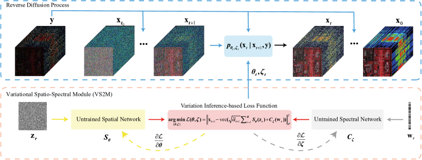
Figure 19: An overview of the self-supervised DDS2M in[141].

Hyperspectral imaging. HSI is a crucial modality in remote sensing with widespread applications. However, due to the limitations of imaging devices, HSIs suffer from data-hungry, noise corruption, and low spatial resolution. Zhang et al.[142] train the first DM conditioned on RGB natural images for HSI generation. The authors employ a spectral folding technique to achieve spectral-to-spatial mapping, addressing the convergence challenges associated with the large spatial sampling space of HSI images due to their high channel count. Deng et al.[143] propose a DM-based model for HSI denoising, utilizing random masking, resembling the one in [131], to balance the importance of spatial and spectral information for performance improvement.

As shown in Fig. 19, Miao et al.[141] introduce an innovative self-supervised DM, DDS2M, for HSI restoration, addressing the data-hungry issue. DDS2M leverages the variational spatio-spectral module, comprising two untrained networks, each focusing on the spatial and spectral dimensions, to exploit the intrinsic structural information of the underlying HSIs. By introducing prior information, DDS2M can learn the posterior distribution solely using the degraded HSI without extra training data. Experiments on HSI denoising, noisy HSI completion, and super-resolution verify the superiority of DDS2M. DDS2M provides new insight into integrating existing DMs with untrained networks and offers a promising solution for HSI restoration.

The spatial and spectral resolutions of spectral images are often challenging to balance due to limitations in imaging technology. Wu et al.[129] propose HSR-Diff, the first diffusion model for HSI Super-resolution (HSR). The model fuses high-resolution multispectral images (MSI) with low-resolution hyperspectral images (LR-HSI) to obtain HR-HSI. The conditional DDPM uses the Conditional Denoising Transformer (CDFormer), which replaces the time embedding with noise embedding, designing spatio-spectral transformer layers designed for HSI characteristics. Shi et al.[130] employ a similar approach and demonstrate the effect of DM-based models on multiple remote sensing datasets.

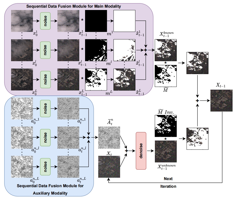
Figure 20: A summary of the conditional inference approach in training and inferential strategies based on sequences.[134].

Synthetic Aperture Radar. Tuel et al.[144] pioneer the use of diffusion models for radar remote sensing imagery, achieving tasks related to SAR image generation and denoising. This method highlights, due to limited data, the lack of powerful feature extractors specific to remote sensing data as a major bottleneck for high-quality generation. Speckle, a type of signal-dependent multiplicative noise affecting coherent imaging modalities including SAR images, is addressed by Perera et al.[132], who introduce DDPM to SAR despeckling. Besides, a new inference strategy based on cycle spinning is proposed to further improve performance. Xiao et al.[133] transform multiplicative noise into traditional additive noise through operations in the logarithmic domain for DM-based denoising. This method introduces patch shifting and averaging-based algorithm similar to[139] to adapt to inputs of arbitrary resolutions, further enhancing performance, albeit increasing computational burden.

Muti-modal remote sensing data. SAR images are robust to weather conditions but are hard to interpret, lacking intuitive visual clarity. In the remote sensing domain, SAR often collaborates with other modalities to accomplish cloud removal tasks. Similarly, in DM-based models, compared to simply modeling cloud removal tasks as inpainting tasks, results with SAR as auxiliary input often exhibit higher credibility. Jing et al.[8] introduce an innovative approach for cloud removal in optical satellite images with DDPM Feature-Based Network for Cloud Removal (DDPM-CR). This model incorporates auxiliary SAR data and multilevel features from the DDPM architecture to recover missing information across various scales. The cloud removal head, equipped with an attention mechanism, recovers missing information, and a cloud-oriented loss balances information recovery in cloud-covered and cloud-free regions. Zhao et al.[134] further integrate multi-temporal sequence information into DM-based models in Fig. 20, amalgamating two mainstream cloud removal concepts in a single framework.

Seo et al.[136], employing a self-supervised denoiser in the latent space, train the Brownian-Bridge diffusion model to achieve SAR to Electro-Optical image translation tasks. Experiments conducted around flood datasets verify enhanced visual information and downstream segmentation task performance for the translated images.

4.3 Diffusion models for video processing

The latest research endeavors aim to extend the exploration of DMs into higher-dimensional data, particularly in video tasks [145, 146, 147, 148, 149]. However, compared with image, video processing requires temporal consistency across video frames. Currently, the number of DM-based video models are relatively few, only applied in several fundamental tasks, including video frame prediction [6], interpolation [150, 151, 152], super-resolution [153, 154], and restoration [155].

Figure 21: The architecture of the two-stage hybrid models [6].

Video frame prediction and interpolation. Renowned for remarkable generative capacities, DM-based models are especially suitable for video prediction and interpolation. Yang et al.[6] first use DMs in autoregressive video prediction. Aiming to model residuals in video compression, the two-stage hybrid model (see in Fig. 21) initially utilizes RNNs to obtain deterministic predictions for the next frame, providing sequential priors for the DM. Then the DM focuses on modeling residuals, whose effect is verified with various metrics perceptually and probabilistically.

By employing different mask manners for time-series, masked conditional DMs can be trained for prediction and interpolation. Höppe et al. [152] introduce conditions through a randomized masking schedule, also allowing the model to be trained conditionally with only slight modifications to the unconditionally trained models. Voleti et al.[150] employ a similar masking concept but further propose a blockwise autoregressive conditioning procedure to facilitate coherent long-term generation. They also incorporate temporal information into the U-Net architecture. In contrast to direct modifications of DDPM, Danier et al.[151] first use LDM in video frame interpolation. They design a vector-quantized autoencoding model for LDM, better recovering high-frequency details and achieving perceptual superiority.

Video super-resolution. Early DM-based video works [146, 147] merely tailor the classical framework to meet data dimensionality of input-output sequences and train the models from scratch, resulting in an undeniable computational burden. Given the tremendous success of DMs [26], one approach is to leverage off-the-shelf pre-trained models and endow them with temporal modeling capacities by integrating temporal layers into the U-Net architecture. Inspired by such works [145, 148, 150], Yuan et al. [154] propose an efficient DM-based method for text-to-video super-resolution. By inflating text-to-image (T2I) model weights into the video generation framework and incorporating an attention-based temporal adapter for coherence across frames, this method achieves high-quality and temporally consistent results.

Striving for Spatial Adaptation and Temporal Coherence (SATeCo), Chen et al. [153] propose a novel video SR approach SATeCo (see in Fig. 22), which freezes pre-trained parameters and optimizes spatial feature adaptation (SFA) and temporal feature alignment (TFA) modules. Specifically, SFA modulates the pixel-level high-resolution features for spatial adaptation through learning affine parameters guided by low-resolution videos. TFA conducts self-attention to enhance feature interaction and further performs cross-attention between counterparts of different resolutions to guide temporal feature alignment learning. Experiments validate the effect of the modules in preserving spatial fidelity and enhancing temporal feature alignment.

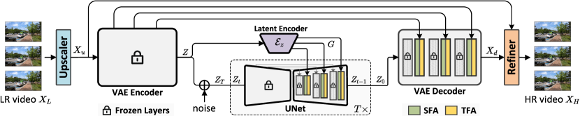
Figure 22: The architecture of SATeCo proposed in [153].

Video restoration. Limited DM-based algorithms focus on video restoration, showing a promising future direction. Yang et al. [155] propose a novel Diffusion Test-Time Adaptation (Diff-TTA) method for all-in-one adverse weather removal in videos. At the training stage, a novel temporal noise model is introduced to exploit frame-correlated information in degraded video clips. During inference, the authors first introduce test-time adaptation to DM-based methods by proposing a novel proxy task named Diffusion Tubelet Self-Calibration (Diff-TSC). This allows the model to adapt in real-time without modifying the training process and achieve restoration under unseen weather conditions.

5 EXPERIMENTS

5.1 Datasets

TABLE I: Datasets for low-level vision tasks. In the column of scales, we present detailed separation information if the dataset is separated as the training and testing sets. Clicking on the dataset will redirect you to its download link.

Tasks	Datasets	Scales	Sources	Modalities	Remarks
SR	BSD500 [156]	500	TPAMI 2010	Syn	A synthetic benchmark that is initially designed for object contour detection.
	Set14 [157]	14	TPAMI 2015	Syn	Commonly utilized for testing performance of super-resolution algorithms.
	Manga109 [158]	109	MTAP 2015	Syn	Compiled mainly for academic research on Japanese manga media processing.
	General100 [159]	100	ECCV 2016	Syn	Synthesized images in uncompressed BMP format covering various scales.
	DIV2K [19]	900/100	NTIRE 2018	Real	A commonly-used dataset with diverse scenarios and realistic degradations.
	Flickr1024 [160]	1024	ICCVW 2019	Syn	A large-scale stereo image dataset with high-quality pairs and diverse scenarios.
	Urban100 [161]	100	CVPR 2019	Syn	Sourced from urban environments: city streets, buildings, and urban landscapes.
	DRealSR [162]	31970	ECCV 2020	Real	Benchmarks captured by DSLR cameras, circumventing simulated degradation.
Deblur	GoPro [20]	2103/1111	CVPR 2017	Syn	Acquired by high-speed cameras for video quality assessment and restoration.
	HIDE [163]	8422	ICCV 2019	Syn	Cover long-distance and short-distance scenarios degraded by motion blur.
	REDS [164]	270/30	NTIRE 2019	Real	Contain 300 video sequences with dynamic duration and varied resolutions.
	BSD [165]	80/20	ECCV 2020	Real	Comprise more scenes and use the proposed beam-splitter acquisition system.
	RealBlur [166]	3758/980	ECCV 2020	Real	Cover common instances of motion blur, captured in raw and JPEG formats.
Dehaze	I-Haze [167]	35	NTIRE 2018	Real	Indoor dataset with real haze for objective image dehazing and evaluation.
	O-Haze [168]	45	NTIRE 2018	Real	Outdoor dataset with real haze for objective image dehazing and evaluation.
	Dense-Haze [169]	33	ICIP 2019	Real	Real-world dataset with dense haze for robust single image dehazing methods.
	RESIDE [170]	13000/990	TIP 2019	Syn+Real	Divided into five subsets to highlight diverse sources and heterogeneous contents.
	NH-Haze [171]	55	CVRPW 2020	Real	The first non-homogeneous dehazing dataset with realistic haze distribution.
	Haze-4K [172]	4000	MM 2021	Syn	A large-scale synthetic dataset for image dehazing with varing distributions.
LLIE	MIT-Fivek [173]	4500/500	CVPR 2011	Syn	A curated dataset of RAW photos adjusted by skilled retouchers for visual appeal.
	LOLv1 [174]	485/15	BMVC 2018	Real	The first dataset with image pairs from real scenarios for low-light enhancement.
	SID [175]	5094	CVPR 2018	Real	A dataset of raw short-exposure images with their long-exposure reference images.
	SICE [176]	589	TIP 2018	Syn	A large-scale multi-exposure image dataset with complex illumination conditions.
	ExDark [177]	7363	CVIU 2019	Real	Collected in low-light scenarios with 12 classes and instance-level annotations.
	LOLv2-Real [178]	689/100	TIP 2021	Real	A three-step shooting strategy is used to eliminate intra-pair image misalignments.
	LOLv2-Syn [178]	900/100	TIP 2021	Syn	Synthetic dark images mimic real low-light photography via histogram analysis.
	SDSD-Indoor [179]	62/6	ICCV 2021	Real	Indoor dataset collected from dynamic scenes under varying lighting conditions.
	SDSD-Outdoor [179]	116/10	ICCV 2021	Real	Outdoor dataset collected from dynamic scenes under varying lighting conditions.
Derain	Rain100H [180]	1800/100	CVPR 2017	Syn	Comprise synthetic datasets with five types of rain streaks for rain removal.
	RainDrop [181]	861/239	CVPR 2018	Syn	Image pairs with raindrop degradation, captured using the setup of dual glasses.
	SPA-Data [182]	638492/1000	CVPR 2019	Real	Design a semi-automatic method to generate clean images from real rain streaks.
	MPID [183]	3961/419	CVPR 2019	Syn+Real	A large-scale benchmark that focuses on driving and surveillance scenarios.
	RainCityscapes [184]	9432/1188	CVPR 2019	Syn	A famous rain removal dataset with paired depth maps for outdoor scenarios.
	RainDS [185]	3450/900	CVPR 2021	Syn+Real	A hybrid dataset with both real and synthesized data under diverse scenarios.
	RainDirection [186]	2920/430	ICCV 2021	Syn	A large-scale synthetic rainy dataset with directional labels in the training phase.
	GT-RAIN [187]	28217/2100	ECCV 2022	Real	The first paired derain dataset with real data by controlling non-rain variations.
Desnow	Snow100k [188]	100000	TIP 2018	Syn+Real	A large-scale dataset with over 1k real-world images degraded by heavy snow.
	SRRS [189]	16000	ECCV 2020	Syn+Real	A hybrid snow dataset with 15k synthesized images and 1k real-world images.
	CSD [190]	10000	ICCV 2021	Syn	A large-scale desnowing dataset to comprehensively simulate snow scenarios.

Large-scale datasets for model pre-training. Constructing DMs from scratch has a rigorous training process, requiring great computation capacities and high-memory hardware that are beyond the reach of many research labs [191]. Hence, using pre-trained models is a common practice in generative modeling tasks, despite the associated risk of potential data leakage[192, 193, 194]. Several commonly used large-scale datasets for pre-training are compiled as:

• ImageNet [59] is a large-scale dataset with over 14 million natural images spanning over 21k classes, termed ImageNet21K. ImageNet1k, serving as a subset of ImageNet21K, has 1k classes with about 1k images per class.

• CelebA [195] has 200k facial images, each annotated with 40 attributes, where CelebA-HQ[196] is a subset having 30k high-resolution facial images.

• LSUN [197] includes 10 scene categories and 20 object categories, each having about 1 million labeled images, typically compressed to JPEG image quality of 75.

• FFHQ [198] comprises 70k high-resolution facial images with diverse distributions. Existing methods based on pre-trained DMs undergo training on FFHQ and evaluation on CelebA-HQ to showcase their generalizability.

TABLE II: Results of DM-based 4$\times$ SR methods.

		DIV2K [19]			Urban100 [161]
Methods	Sources	PSNR$\uparrow$	SSIM$\uparrow$	LPIPS$\downarrow$	PSNR$\uparrow$	SSIM$\uparrow$	LPIPS$\downarrow$
Bicubic	—	25.36	0.643	0.31	24.26	0.628	0.34
IR-SDE [82]	ICML2023	25.90	0.657	0.23	26.63	0.786	0.18
CDPMSR [199]	ICIP2023	27.43	0.712	0.19	26.98	0.801	0.16
IDM [9]	CVPR2023	27.13	0.703	0.18	26.76	0.657	0.13
DiffIR [4]	ICCV2023	29.13	0.730	0.09	26.05	0.776	0.10
ResDiff [200]	AAAI2024	27.94	0.723	0.23	27.43	0.824	0.14

TABLE III: Results of DM-based motion deblurring methods.

		Gopro [20]			HIDE [163]
Methods	Sources	PSNR$\uparrow$	SSIM$\uparrow$	LPIPS$\downarrow$	PSNR$\uparrow$	SSIM$\uparrow$	LPIPS$\downarrow$
Blurred image	—	25.64	0.793	0.29	23.95	0.763	0.33
DSR [83]	CVPR2022	33.23	0.963	0.08	30.07	0.928	0.09
IR-SDE [82]	ICML2023	30.70	0.901	0.06	28.34	0.914	0.10
MSGD [10]	ICCV2023	31.19	0.943	0.06	29.14	0.910	0.09
HI-Diff [90]	NIPS2023	33.33	0.964	0.08	31.46	0.945	0.11
DiffEvent [93]	ICASSP2024	35.55	0.972	0.06	—	—	—

TABLE IV: Results of DM-based low-light enhancement methods (* means using the gt mean strategy in the inference stage.).

		LOLv1[174]			LOLv2 Real [178]			LOLv2 Syn [178]
Methods	Sources	PSNR$\uparrow$	SSIM$\uparrow$	LPIPS$\downarrow$	PSNR$\uparrow$	SSIM$\uparrow$	LPIPS$\downarrow$	PSNR$\uparrow$	SSIM$\uparrow$	LPIPS$\downarrow$	Parameters(M)$\downarrow$	MACs(G)$\downarrow$
Low-Light Image	—	7.77	0.193	0.56	9.71	0.210	0.52	11.22	0.447	0.38	N/A	N/A
PyDiff*[96]	IJCAI2023	27.09	0.936	0.10	24.01	0.876	0.23	19.60	0.878	0.22	97.89	459.69
Diff-Retinex[106]	ICCV2023	21.98	0.852	0.048	20.17	0.826	0.10	24.30	0.921	0.06	56.88	396.32
GSAD*[105]	NIPS2023	27.83	0.877	0.09	28.82	0.895	0.09	28.67	0.944	0.04	17.17	1340.63
LLDiffusion[104]	arXiv2023	24.65	0.843	—	23.16	0.842	—	25.99	0.948	—	—	—
Reti-Diff[7]	arXiv2023	25.35	0.866	0.09	22.97	0.858	0.08	27.53	0.951	0.03	26.11	156.55

Low-level vision datasets for model training. Various datasets are tailored to address diverse low-level vision tasks, aiming to accommodate various degradation modes. Due to space limitations, we provide a summary of commonly used datasets for several classical natural low-level vision tasks in Table I, including their scales, sources, modalities, and remarks. For more information about datasets in different scenarios, please refer to our repository. In practice, DM-based models are typically pre-trained on large-scale datasets to learn general features and structures, before being fine-tuned on specific low-level vision datasets to address the specific degradation issues.

5.2 Evaluation metrics

5.2.1 Distortion-based metrics

• PSNR [7] (Peak Signal to Noise Ratio) quantifies the pixel-wise disparity between a corrupted image and its clean image by computing their mean squared error.

• SSIM (Structural Similarity [201]), aiming to accommodate human visual perception, assesses the likeness between distorted and clean images across three aspects, including contrast, brightness, and structure.

5.2.2 Inception-based metrics

• LPIPS (Learned Perceptual Image Patch Similarity [202]), is a learning-based metric that leverages the pre-trained AlexNet as a feature extractor and adjusts the linear layer to emulate human perception.

• FID (Fréchet inception distance [203]) assesses the fidelity and diversity of generated images by computing the Fréchet distance of their reference images.

• KID (Kernel Inception Distance [204]), similar to FID, employs maximum mean discrepancy with a polynomial kernel to measure the distance, showing greater stability in the zero-shot and few-shot conditions.

• NIQE (Natural Image Quality Evaluator [205]), a no-reference metric, evaluates the distance between the natural scene statistics of distorted images and natural images modeled with a multivariate Gaussian model.

5.2.3 Human-centric evaluations

Human-centric evaluation serves as a primary subjective assessment method, where participants select the image verifying the most effective performance from a set of images. To ensure fairness, anonymizing the method and randomizing the order of images within each set are essential practices. Typically, human assessment scores are calculated using the Mean Opinion Score (MOS) derived from a pool of participants. A higher MOS indicates superior perceptual quality as perceived by humans. However, evaluating via MOS can be costly, and the results may be biased due to subjective perceptual differences. Besides, the time-consuming nature of the procedure makes it suitable for small-scale assessments, such as user studies, but challenging to employ for evaluation during training and broader comparisons.

5.2.4 Downstream application-based evaluations

Apart from improving visual quality, generating those enhanced images that can facilitate high-level vision tasks, such as object recognition and image segmentation[12, 21], is also a significant object. Hence, the evaluation of various methods extends to examining the impact of low-level vision methods on real-world vision-based applications.

5.3 Experimental results

We provide quantitative comparisons for DM-based methods on three commonly investigated tasks.

Results on super-resolution. The results for DM-based models on 4$\times$ image super-resolution, tested on DIV2k [19] and Urban100 [161], are listed in Table III. We find that IDM [9] and DiffIR [4] perform well on LPIPS. They leverage preprocessed images or features as conditional input, which are demonstrated to enhance perceptual quality. In contrast, Resdiff [200] performs well on PSNR and SSIM. This is because Resdiff uses DM to estimate residual information, ensuring the salient consistency of the restored image with the high-resolution image.

Results on deblurring. We evaluate five DM-based methods on the motion deblurring task using the Gopro [20] and HIDE [163] datasets and report The results in Table III. We can find that DiffEvent [93] and HI-Diff [90] achieve competitive performance on PSNRs and SSIMs. DiffEvent is enabled to achieve both low-light recovery and image deblurring by introducing a learnable decomposer. HI-Diff achieves good generalization performance in complex fuzzy scenarios by using LDM to generate a highly-compressed prior. Moreover, MSGD [10] introduces a multi-scale structural bootstrap to better sample from the target condition distribution, hence the best performance on perceptual metrics.

Results on low-light image enhancement. We validate the performance of five DM-based methods on the low-light image enhancement task using the LOLv1 [174], LOLv2 Real [178], and LOLv2 Syn [178] datasets. The results, presented in Table IV, demonstrate that GSAD [105] shows superior performance in terms of PSNR. Pydiff[96] performs exceptionally well on LOLv1 Dataset with a roughly 6% improvement over other diffusion models in terms of SSIM. Reti-Diff [7] achieves competitive performance in terms of LPIPS [202]. In terms of model parameters and computational complexity, GSAD significantly outperforms other methods on parameters, but introduces a huge computational complexity. Benefiting from using LDM within a low-dimensional compact space, Reti-Diff has the second smallest parameter count and the lowest MACs. Noting that GSAD [105] and PyDiff [96] employ the ”gt mean” strategy, which involves fine-tuning the brightness of the generated results using the ground truth, thus producing much more impressive results than others in PSNR and SSIM.

6 Future directions

Compared to other generative models, DMs exhibit the capability to generate high-fidelity images with complex details, rendering DMs widely applied in low-level vision tasks. However, considerable room for advancement remains in both DMs and low-level vision tasks.

In this section, we primarily focus on three avenues to enhance the influence of DMs in low-level vision tasks: (1) Mitigating the limitations of DMs, (2) Amalgamating the strengths of DMs with the traits of low-level vision, and (3) Tackling the inherent challenges of low-level vision.

6.1 Mitigating the limitations of DMs

Due to the high computational overhead, DMs encounter barriers to be applied in low-level vision tasks. Two viable ways are listed and discussed to mitigate this challenge.

Reducing sample steps. Various efforts, extending beyond low-level vision, have been undertaken to enhance the sampling efficiency of DM: (1) Modeling the diffusion process with a non-Markov Chain, such as DDIM[24]. (2) Designing efficient ODE solvers [46]. (3) Using knowledge distillation to reduce sampling steps[206, 207]. (4) Performing DMs on compressed latent spaces [26]. (5) Introducing cross-modality priors with conditional mechanisms[208, 209].

With these efforts, the number of sampling steps has been notably reduced to 10-20 steps, ensuring faster reconstruction. For instance, DDRM [64] achieves an inference time reduction to 8 seconds for a single $224\times 224$ image by using the sampling strategy of DDIM [24]. Besides, some studies[70, 210] initialize networks by sampling from low-quality images or one-step reconstruction results of baseline networks, streamlining the learning target.

However, despite notable progress, the overall computational cost remains high, particularly for high-resolution images, presenting a substantial gap from real-time applications. Addressing this challenge remains a longstanding and crucial direction for accelerating diffusion models.

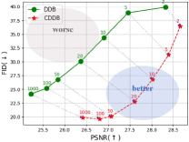
(a) Shift in pareto-frontier[69].

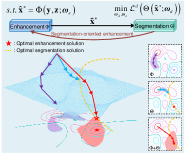
(b) Bi-level optimization[21].

Figure 23: Two strategies to amalgamate the strengths of DMs with the traits of low-level vision in Sec. 6.2.

Compressing model consumption. The deployment of DM-based models in low-resource environments, such as edge devices, faces challenges due to their immense parameter size and computational complexity. Apart from employing fewer-step inference, researchers can explore architectural optimizations to address this issue, including model quantization, pruning, and knowledge distillation. Zhang et al. [211] combine automated layer pruning with normalized feature distillation to compress models. Castells et al. [212] propose EdgeFusion, an optimized model for deploying SDMs on Neural Processing Units, which leverages advanced distillation techniques and model-level tiling to facilitate rapid inference. However, current methods primarily focus on generation tasks. In the future, these techniques are expected to be extended to low-level vision tasks, leveraging specific properties of each task for model compression.

6.2 Amalgamating the strengths of DMs with the traits of low-level vision

The greatest trait of low-level vision lies in the diversity of evaluation criteria, including visual fidelity, content invariance, and downstream task-based evaluations. DM-based methods, generating visual fidelity results, also should ensure the content invariance of the original one and the generated result and facilitate downstream tasks.

Perception-distortion trade-off. DM-based methods generate visually appealing results and excel in inception-based metrics, such as LPIPS[202] and FID[203]. However, their high diversity often leads to challenges in maintaining content consistency, resulting in suboptimal performance in those distortion-based metrics such as PSNR and SSIM.

One potential solution involves designing hybrid models that integrate DMs with CNN-based or Transformer-based frameworks [7, 4]. These hybrid models have shown promising results, particularly in improving distortion-based metrics. Besides, Pareto-frontiers are introduced as a comprehensive indicator to evaluate both perception and distortion and have proven the positive shift of the multiscale guidance mechanism [69] that enhances coarse sharp image structures (in Fig. 23 (a)). However, breakthrough progress has not yet been made and further explorations about novel mixed structure and new metrics are expected.

Downstream task-friendly designs. Enabling reconstructed images to better serve downstream tasks is a continuous endeavor in low-level vision research[41]. This pursuit manifests in three primary approaches with DMs.

First, as shown in Fig. 23 (b), several strategies [21, 213] adopt bi-level optimization to jointly optimize the networks of both the low-level vision task and the downstream task, such as image segmentation and object detection. By jointly optimizing the enhancement network with constraints from both itself and the downstream task, these methods aim to produce visually appealing results while enhancing downstream performance. Besides, Ju et. al [214] propose feature-level information aggregation between low-level vision tasks and downstream tasks instead of the previous image-level manner, improving performance with deep constraints. Inspired by the adversarial attacks, which introduce slight perturbations to cause original methods to fail, Sun et. al[215] propose adding slight noise to dehazed images. This strategy enhances downstream detection performance without altering the visual outcome. However, these methods are often tailored to specific downstream tasks. There remains a need for a unified strategy, especially DM-based solutions that can generate visually friend results, to optimize generated images for a wide range of downstream tasks, which awaits further exploration.

6.3 Tackling the inherent challenges of low-level vision

Low-level vision tasks have several inherent challenges, including generalizability, data volume and controllability.

Real-world image restoration. Two ways can help DM-based methods to address real-world scenarios, i.e., distortion invariant learning (DIL) and distortion estimation (DE).

DIL, renowned for its degradation-invariant representation and structural information preservation[216], can enhance DM-based methods by incorporating a distortion-invariant noise predictor and condition. This enables these methods to generalize effectively to diverse and even unknown degradations. Pioneering efforts have focused on redesigning the condition module to achieve distortion-invariant conditions, as demonstrated in works such as DifFace [217] and DR2 [81]. Notably, the effectiveness of such conditions also relies on DIL, warranting further research.

Moreover, DE techniques, extracting prior knowledge of degradation processes, are also urgently needed to extend the zero-shot diffusion models to real-world applications. Even though explicit results cannot be obtained, the powerful image synthesis capability of DMs can be utilized to convert synthetic datasets into real-world paired datasets, which will be discussed in detail in the following subsection.

Data generation for data-hungry fields. Data hungry is a prevalent challenge in low-level tasks, often stemming from limitations inherent in imaging devices and scenarios.

While the unsupervised training is one avenue, many existing approaches [21] resort to data generation strategies to create pseudo image pairs. These pairs typically consist of generated degraded low-quality images paired with their corresponding original high-quality counterparts. This is a promising way for DM-based methods, although with limited explorations, for their powerful generation capacity. Moreover, certain extreme tasks suffer from severely limited data availability due to the difficulty or costliness of data acquisition, as seen in Photoacoustic data[218] and Cryo-electron microscopy data[219]. He et. al [57] propose leveraging existing data to generate more training data with GAN and thus enhance the generalizability of the method. This strategy aligns well with the DM-based methods, offering stable training conditions. Furthermore, controllable data generation, facilitated by user interaction, presents a promising approach to filtering out negative data that could otherwise affect stable performance.

Controllable and interactive low-level vision. Enhancing the controllability of low-level vision methods, enabling them to discern what and where users desire recovery, is of paramount importance. This focus has persisted over time, with efforts including the integration of human perception-related loss functions [220] and interactive guidance priors [21]. Recently, the utilization of vision prompts facilitated by Vision-Language models [221] has provided a means for existing low-level vision methods to explicitly incorporate and interact with prompts within their networks, thereby achieving improved control and restoration effects [222]. Given that these vision prompts can act as interactive priors to curb the excessive diversity inherent in DM-based methods, leveraging Vision-Language models to develop controllable and interactive DM-based methods shows promise.

Moreover, future efforts should address real-world scenarios that involve multiple degradations. Zheng et al. [223] introduce a novel DM-based method named DiffUIR, employing a selective hourglass mapping technique. Instead of relying on prompt learning methods, DiffUIR combines shared distribution mapping and robust conditional guidance based on Residual Denoising Diffusion Models [224] to improve image restoration performance. Improving the internal mechanisms of deep learning to better learn the distribution of multi-task degradations represents a promising direction for future DM-based explorations.

7 Conclusions

In this survey, we offer an extensive examination of denoising diffusion models applied in low-level vision tasks, a gap overlooked in previous surveys. Our review covers both advances and practical implementations in this domain. Firstly, we identify and discuss various generic diffusion modeling frameworks. We then propose a comprehensive categorization of diffusion models utilized in low-level vision tasks from multiple perspectives. Lastly, we highlight the limitations of existing diffusion models and suggest intriguing avenues for future research and explorations. Advancements in low-level vision tasks using these models are emerging in more complex and higher-dimensional mediums, including 3D objects, locomotion, and 4D scenes, warranting sustained attention in future research.

References

- [1] Z. Wang, J. Chen, and S. C. Hoi, “Deep learning for image super-resolution: A survey,” IEEE Trans. Pattern Anal. Mach. Intell., vol. 43, no. 10, pp. 3365–3387, 2020.
- [2] S. Biyouki and H. Hwangbo, “A comprehensive survey on deep neural image deblurring,” arXiv preprint arXiv:2310.04719, 2023.
- [3] Y. Liu, G. Zhao, B. Gong, Y. Li, R. Raj, and N. Goel, “Improved techniques for learning to dehaze and beyond: A collective study,” arXiv preprint arXiv:1807.00202, 2018.
- [4] B. Xia, Y. Zhang, S. Wang, and Y. Wang, “Diffir: Efficient diffusion model for image restoration,” arXiv arXiv:2303.09472, 2023.
- [5] C. He, K. Li, G. Xu, Y. Zhang, R. Hu, Z. Guo, and X. Li, “Degradation-resistant unfolding network for heterogeneous image fusion,” in ICCV, pp. 12611–12621, 2023.
- [6] R. Yang, P. Srivastava, and S. Mandt, “Diffusion probabilistic modeling for video generation,” CoRR, vol. abs/2203.09481, 2022.
- [7] C. He, C. Fang, Y. Zhang, K. Li, L. Tang, and Z. Guo, “Reti-diff: Illumination degradation image restoration with retinex-based latent diffusion model,” arXiv preprint arXiv:2311.11638, 2023.
- [8] R. Jing, F. Duan, F. Lu, M. Zhang, and W. Zhao, “Denoising diffusion probabilistic feature-based network for cloud removal in sentinel-2 imagery,” Remote Sens., vol. 15, no. 9, p. 2217, 2023.
- [9] S. Gao, X. Liu, and B. Zeng, “Implicit diffusion models for continuous super-resolution,” in CVPR, pp. 10021–10030, 2023.
- [10] M. Ren, M. Delbracio, and H. Talebi, “Multiscale structure guided diffusion for image deblurring,” in ICCV, pp. 10721–10733, 2023.
- [11] A. Lugm, M. Danel, and F. Yu, “Repaint: Inpainting using denoising diffusion probabilistic models,” in CVPR, pp. 61–71, 2022.
- [12] J. Liu and R. Anirudh, “A model-based probabilistic diffusion framework for limited-angle ct reconstruction,” in ICCV, 2023.
- [13] C. Saxena and D. Kourav, “Noises and image denoising techniques: a brief survey,” IJEATE, vol. 4, no. 3, pp. 878–885, 2014.
- [14] C. He, X. Wang, and L. Deng, “Image threshold segmentation based on glle histogram,” in CPSCom, pp. 410–415, IEEE, 2019.
- [15] C. He, K. Li, Y. Zhang, L. Tang, Y. Zhang, Z. Guo, and X. Li, “Camouflaged object detection with feature decomposition and edge reconstruction,” in CVPR, pp. 22046–22055, 2023.
- [16] C. He, K. Li, Y. Zhang, G. Xu, and L. Tang, “Weakly-supervised concealed object segmentation with sam-based pseudo labeling and multi-scale feature grouping,” NeurIPS, 2024.
- [17] J. Su, B. Xu, and H. Yin, “A survey of deep learning approaches to image restoration,” Neurocomputing, vol. 487, pp. 46–65, 2022.
- [18] A. M. Ali, B. Benjdira, and A. Koubaa, “Vision transformers in image restoration: A survey,” Sensors, p. 2385, 2023.
- [19] E. Agustsson and R. Timofte, “Ntire17 challenge on single image super-resolution: Dataset and study,” in CVPRW, 2017.
- [20] S. Nah and T. Hyun Kim, “Deep multi-scale convolutional network for dynamic scene deblurring,” in CVPR, pp. 883–891, 2017.
- [21] C. He, K. Li, G. Xu, J. Yan, and L. Tang, “Hqg-net: Unpaired medical image enhancement with high-quality guidance,” IEEE Trans. Neural Netw. Learn. Syst., 2023.
- [22] J. Sohl-Dickstein and E. Weiss, “Deep unsupervised learning using nonequilibrium thermodynamics,” in ICML, 2015.
- [23] Y. Song and S. Ermon, “Generative modeling by estimating gradients of the data distribution,” NeurIPS, 2019.
- [24] J. Song, C. Meng, and S. Ermon, “Denoising diffusion implicit models,” arXiv preprint arXiv:2010.02502, 2020.
- [25] J. Ho, A. Jain, and P. Abbeel, “Denoising diffusion probabilistic models,” NeurIPS, pp. 6840–6851, 2020.
- [26] R. Rombach and A. Blattmann, “High-resolution image synthesis with latent diffusion models,” in CVPR, pp. 684–695, 2022.
- [27] A. Q. Nichol and P. Dhariwal, “Improved denoising diffusion probabilistic models,” in ICML, pp. 8162–8171, PMLR, 2021.
- [28] Y. Song and J. Sohl, “Score-based generative modeling through stochastic differential equations,” arXiv arXiv:2011.13456, 2020.
- [29] D. Watson and W. Chan, “Learning fast samplers for diffusion models by differentiating through sample quality,” in ICLR, 2021.
- [30] P. Dhariwal and A. Nichol, “Diffusion models beat gans on image synthesis,” NeurIPS, pp. 8780–8794, 2021.
- [31] O. Özdenizci and R. Legenstein, “Restoring vision in adverse weather conditions with patch-based denoising diffusion models,” IEEE Trans. Pattern Anal. Mach. Intell., 2023.
- [32] Z. Luo, F. K. Gustafsson, Z. Zhao, J. Sjölund, and T. B. Schön, “Refusion: Enabling large-size realistic image restoration with latent-space diffusion models,” in CVPR, pp. 1680–1691, 2023.
- [33] F.-A. Croitoru and V. Hondru, “Diffusion models in vision: A survey,” IEEE Trans. Pattern Anal. Mach. Intell., 2023.
- [34] L. Yang, Z. Zhang, Y. Song, S. Hong, R. Xu, Y. Zhao, W. Zhang, B. Cui, and M.-H. Yang, “Diffusion models: A comprehensive survey of methods and applications,” ACM Comput. Surv., 2022.
- [35] C. Zhang and C. Zhang, “Text-to-image diffusion model in generative ai: A survey,” arXiv preprint arXiv:2303.07909, 2023.
- [36] Y. Huang, J. Huang, Y. Liu, and M. Yan, “Diffusion model-based image editing: A survey,” arXiv preprint arXiv:2402.17525, 2024.
- [37] S. Parida, V. Srinivas, B. Jain, and R. Naik, “Survey on diverse image inpainting using diffusion models,” in PCEMS, 2023.
- [38] B. B. Moser, A. S. Shanbhag, F. Raue, S. Frolov, S. Palacio, and A. Dengel, “Diffusion models, image super-resolution and everything: A survey,” arXiv preprint arXiv:2401.00736, 2024.
- [39] X. Li and Y. Ren, “Diffusion models for image restoration and enhancement–a survey,” arXiv preprint arXiv:2308.09388, 2023.
- [40] J. Wang and Z. Yue, “Exploiting diffusion prior for real-world image super-resolution,” arXiv preprint arXiv:2305.07015, 2023.
- [41] C. Saharia and J. Ho, “Image super-resolution via iterative refinement,” IEEE Trans. Pattern Anal. Mach. Intell., pp. 713–726, 2022.
- [42] J. Ho, A. Jain, and P. Abbeel, “Denoising diffusion probabilistic models,” NeurIPS, pp. 6840–6851, 2020.
- [43] P. Vincent, “A connection between score matching and denoising autoencoders,” Neural Comput., vol. 23, no. 7, pp. 1661–1674, 2011.
- [44] Y. Song, S. Garg, J. Shi, and S. Ermon, “Sliced score matching: A scalable approach to score estimation,” in UAI, pp. 574–584, 2020.
- [45] B. D. Anderson, “Reverse-time diffusion equation models,” Stochastic Processes Appl., vol. 12, no. 3, pp. 313–326, 1982.
- [46] E. Weinan, “A proposal on machine learning via dynamical systems,” Commun. Math. Stat., vol. 1, no. 5, pp. 1–11, 2017.
- [47] D. P. Kingma and M. Welling, “Auto-encoding variational bayes,” arXiv preprint arXiv:1312.6114, 2013.
- [48] L. Deng, C. He, and G. Xu, “Pcgan: A noise robust conditional generative adversarial network for one shot learning,” IEEE Trans. Intell. Transp. Syst., pp. 25249–25258, 2022.
- [49] K. Pandey and A. Mukherjee, “Vaes meet diffusion models: Efficient and high-fidelity generation,” in NeurIPSW, 2021.
- [50] A. Vahdat, K. Kreis, and J. Kautz, “Score-based generative modeling in latent space. 2021,” arXiv preprint arXiv:2106.05931, 2021.
- [51] L. Dinh and Y. Bengio, “Nice: Non-linear independent components estimation,” arXiv preprint arXiv:1410.8516, 2014.
- [52] L. Dinh, J. Sohl-Dickstein, and S. Bengio, “Density estimation using real nvp,” arXiv preprint arXiv:1605.08803, 2016.
- [53] Q. Zhang and Y. Chen, “Diffusion normalizing flow,” Adv. neural inf. process. syst., vol. 34, pp. 16280–16291, 2021.
- [54] I. Goodfellow, J. Pouget-Abadie, and M. Mirza, “Generative adversarial nets,” NeurIPS, 2014.
- [55] C. Han, K. Murao, T. Noguchi, and Y. Kawata, “Learning more with less: Conditional pggan-based data augmentation for brain metastases detection,” in CIKM, pp. 119–127, 2019.
- [56] T. Karras, S. Laine, and M. Aittala, “Analyzing and improving the image quality of stylegan,” in CVPR, pp. 110–119, 2020.
- [57] C. He, K. Li, Y. Zhang, Y. Zhang, Z. Guo, and X. Li, “Strategic preys make acute predators: Enhancing camouflaged object detectors by generating camouflaged objects,” in ICLR, 2024.
- [58] H. Chung, J. Kim, and Mccann, “Diffusion posterior sampling for general noisy inverse problems,” arXiv arXiv:2209.14687, 2022.
- [59] O. Russakovsky, J. Deng, and H. Su, “Imagenet large scale visual recognition challenge,” Int. J. Comput. Vision, pp. 211–252, 2015.
- [60] G. Batzolis and J. Stanczuk, “Conditional image generation with score-based diffusion models,” arXiv arXiv:2111.13606, 2021.
- [61] J. Choi and S. Kim, “Ilvr: Conditioning method for denoising diffusion probabilistic models,” arXiv arXiv:2108.02938, 2021.
- [62] H. Chung and B. Sim, “Improving diffusion models for inverse problems using manifold constraints,” NeurIPS, pp. 83–96, 2022.
- [63] A. Graikos, N. Malkin, N. Jojic, and D. Samaras, “Diffusion models as plug-and-play priors,” NeurIPS, pp. 14715–14728, 2022.
- [64] B. Kawar, M. Elad, and S. Ermon, “Denoising diffusion restoration models,” NeurIPS, pp. 23593–23606, 2022.
- [65] Y. Zhu, K. Zhang, and J. Liang, “Denoising diffusion models for plug-and-play image restoration,” in CVPR, pp. 1219–1229, 2023.
- [66] Y. Wang and J. Yu, “Zero-shot image restoration using denoising diffusion model,” arXiv preprint arXiv:2212.00490, 2022.
- [67] M. Delbracio and P. Milanfar, “Inversion by direct iteration: An alternative to denoising diffusion for image restoration,” arXiv preprint arXiv:2303.11435, 2023.
- [68] G.-H. Liu, A. Vahdat, and D.-A. Huang, “I2sb: Image-to-image schrodinger bridge,” arXiv preprint arXiv:2302.05872, 2023.
- [69] H. Chung, J. Kim, and J. C. Ye, “Direct diffusion bridge using data consistency for inverse problems,” arXiv preprint arXiv:2305.19809, 2023.
- [70] H. Chung, B. Sim, and J. C. Ye, “Come-closer-diffuse-faster: Accelerating conditional diffusion models for inverse problems through stochastic contraction,” in CVPR, pp. 12413–12422, 2022.
- [71] K. Pandey, A. Mukherjee, P. Rai, and A. Kumar, “Diffusevae: Efficient, controllable and high-fidelity generation from low-dimensional latents,” arXiv preprint arXiv:2201.00308, 2022.
- [72] Z. Fabian, B. Tinaz, and M. Soltanolkotabi, “Diracdiffusion: Denoising and incremental reconstruction with assured data-consistency,” arXiv preprint arXiv:2303.14353, 2023.
- [73] Z. Yue and J. Wang, “Efficient diffusion model for image restoration by residual shifting,” arXiv preprint arXiv:2403.07319, 2024.
- [74] H. Li, Y. Yang, and M. Chang, “Srdiff: Single image super-resolution with diffusion models,” Neurocom., pp. 47–59, 2022.
- [75] C. Saharia, J. Ho, W. Chan, and T. Salimans, “Image super-resolution via iterative refinement,” IEEE Trans. Pattern Anal. Mach. Intell., vol. 45, no. 4, pp. 4713–4726, 2022.
- [76] J. Ho, C. Saha, and W. Chan, “Cascaded diffusion models for high fidelity image generation,” J. Mach. Learn. Res., pp. 249–281, 2022.
- [77] A. Niu, K. Zhang, and T. X. Pham, “Conditional diffusion probabilistic models for single image super-resolution,” in ICIP, 2023.
- [78] X. Lin, J. He, and Z. Chen, “Diffbir: Towards blind image restoration with generative diffusion prior,” arXiv:2308.15070, 2023.
- [79] H. Sun and W. Li, “Coser: Bridging image and language for cognitive super-resolution,” arXiv preprint arXiv:2311.16512, 2023.
- [80] S. AlHalawani and B. Benjdira, “License plate super-resolution using diffusion models,” arXiv preprint arXiv:2309.12506, 2023.
- [81] Z. Wang and Z. Zhang, “Dr2: Diffusion-based robust degradation remover for blind face restoration,” in CVPR, pp. 64–73, 2023.
- [82] Z. Luo and F. Gusta, “Image restoration with mean-reverting stochastic differential equations,” arXiv:2301.11699, 2023.
- [83] J. Whang, M. Delbracio, H. Talebi, and C. Saharia, “Deblurring via stochastic refinement,” in CVPR, pp. 293–303, 2022.
- [84] E. Gebre, K. Saxena, and T. Tran, “A diffusion-based image inpainting pipeline,” arXiv preprint arXiv:2403.16016, 2024.
- [85] C. Zhang and W. Yang, “Multi-modality guided image inpainting based on diffusion models,” IEEE Trans. Multimedia, 2024.
- [86] W. Li, X. Yu, and K. Zhou, “Sdm: Spatial diffusion model for large hole image inpainting,” arXiv preprint arXiv:2212.02963, 2022.
- [87] C. Saharia, W. Chan, H. Chang, and C. Lee, “Palette: Image-to-image diffusion models,” in SIGGRAPH, pp. 1–10, 2022.
- [88] X. Ju, X. Liu, and X. Wang, “A plug-and-play image inpainting model with decomposed diffusion,” arXiv:2403.06976, 2024.
- [89] A. Grechka and G. Couairon, “Gradient-guided inpainting with diffusion models,” Comput. Vis. Image Underst., 2024.
- [90] Z. Chen, Y. Zhang, and D. Liu, “Hierarchical integration diffusion model for realistic image deblurring,” NeurIPS, 2023.
- [91] C. Laroche, A. Almansa, and E. Coupete, “Fast diffusion em: a diffusion model for blind inverse problems with application to deconvolution,” in WACV, pp. 5271–5281, 2024.
- [92] R. Spetlik, D. Rozumnyi, and J. Matas, “Single-image deblurring, trajectory and shape recovery of fast moving objects with denoising diffusion models,” in WACV, pp. 6857–6866, 2024.
- [93] P. Wang, J. He, and Q. Yan, “Diffevent: Event residual diffusion for image deblurring,” in ICASSP, pp. 3450–3454, IEEE, 2024.
- [94] F.-A. Vasluianu and T. Seizinger, “Ntire 2023 image shadow removal challenge report,” in CVPR, pp. 1788–1807, 2023.
- [95] J. Wang, S. Wu, and Z. Yuan, “Frequency compensated diffusion model for real-scene dehazing,” Neural Networks, p. 106281, 2024.
- [96] D. Zhou and Z. Yang, “Pyramid diffusion models for low-light image enhancement,” arXiv preprint arXiv:2305.10028, 2023.
- [97] Y. Zhu and L. Wang, “Diffusion model based low-light enhancement for space satellite,” arXiv preprint arXiv:2306.14227, 2023.
- [98] G. Wu and C. Jin, “Difflie: Low-light image enhancment based on deep diffusion model,” in ISCTIS, pp. 522–526, IEEE, 2023.
- [99] C. Nguyen, E. Chan, A. Bergman, and G. Wetzstein, “A diffusion model for low-light text recognition,” in WACV, pp. 46–57, 2024.
- [100] S. Panagiotou and A. S. Bosman, “Denoising diffusion for low-light image enhancement,” arXiv preprint arXiv:2303.09627, 2023.
- [101] H. Jiang, A. Luo, and H. Fan, “Low-light image enhancement with wavelet-based diffusion models,” ACM TOG, pp. 1–14, 2023.
- [102] Y. Wang, Y. Yu, W. Yang, and L. Guo, “Learning to expose for low-light image enhancement,” in ICCV, pp. 12438–12448, 2023.
- [103] X. Lv, X. Dong, and Z. Jin, “L2dm: A diffusion model for low-light image enhancement,” in PRCV, pp. 130–145, 2023.
- [104] T. Wang, K. Zhang, and Z. Shao, “Lldiffusion: Learning degradation representations in diffusion models for low-light image enhancement,” arXiv preprint arXiv:2307.14659, 2023.
- [105] J. Hou, Z. Zhu, and J. Hou, “Global structure-aware diffusion process for low-light image enhancement,” NeurIPS, 2024.
- [106] X. Yi, H. Xu, and J. Ma, “Diff-retinex: Rethinking low-light image enhancement with a generative diffusion model,” in ICCV, 2023.
- [107] Y. Yin and D. Xu, “Cle diffusion: Controllable light enhancement diffusion model,” in ACM MM, pp. 145–156, 2023.
- [108] M. Xue, J. He, and Y. He, “Low-light image enhancement via clip-fourier guided wavelet diffusion,” arXiv:2401.03788, 2024.
- [109] J. Yue, L. Fang, S. Xia, Y. Deng, and J. Ma, “Dif-fusion: Towards high color fidelity in infrared and visible image fusion with diffusion models,” IEEE Trans. Image Process., 2023.
- [110] Z. Zhao, H. Bai, Y. Zhu, and J. Zhang, “Denoising diffusion model for multi-modality image fusion,” in ICCV, pp. 8082–8093, 2023.
- [111] Z. Cao, S. Cao, and X. Wu, “Denoising diffusion model for remote sensing image fusion,” arXiv preprint arXiv:2304.04774, 2023.
- [112] M. Li, R. Pei, and T. Zheng, “Multi-focus image fusion using denoising diffusion models,” Expert Syst. Appl., vol. 238, 2024.
- [113] H. Chung and J. C. Ye, “Score-based diffusion models for accelerated mri,” Med. Image Anal., vol. 80, p. 102479, 2022.
- [114] S. Kumari and P. Singh, “Data efficient deep learning for medical image analysis: A survey,” arXiv preprint arXiv:2310.06557, 2023.
- [115] L. Xu, H. Wu, and C. He, “Multi-modal sequence learning for alzheimer’s disease progression prediction with incomplete variable-length longitudinal data,” Med. Image Anal., 2022.
- [116] L. Tang, K. Li, C. He, Y. Zhang, and X. Li, “Source-free domain adaptive fundus image segmentation with class-balanced mean teacher,” in MICCAI, pp. 684–694, 2023.
- [117] A. Jalal, M. Arvinte, and G. Daras, “Robust compressed sensing mri with deep generative priors,” NeruIPS, pp. 38–54, 2021.
- [118] A. C. Kak and M. Slaney, Principles of computerized tomographic imaging. SIAM, 2001.
- [119] G. Xu, C. He, H. Wang, H. Zhu, and W. Ding, “Dm-fusion: Deep model-driven network for heterogeneous image fusion,” IEEE Trans. Neural Netw. Learn. Syst., 2023.
- [120] Y. Peng, M. Li, and J. Grandi, “Top-level design and simulated performance of first portable ct-mr scanner,” IEEE Access, 2022.
- [121] M. Ju, C. He, and J. Liu, “Ivf-net: An infrared and visible data fusion deep network for traffic object enhancement in intelligent transportation systems,” IEEE Trans. Intell. Transp. Syst., 2022.
- [122] Q. Lyu and G. Wang, “Conversion between ct and mri images using diffusion models,” arXiv preprint arXiv:2209.12104, 2022.
- [123] X. Meng, Y. Gu, and Y. Pan, “A novel unified conditional score-based generative framework for multi-modal medical image completion,” arXiv preprint arXiv:2207.03430, 2022.
- [124] S. Bakas, M. Reyes, and A. Jakab, “Identifying machine learning for brain tumor segmentation overall survival prediction in the brats challenge,” arXiv preprint arXiv:1811.02629, 2018.
- [125] Y. Li, H. Shao, and X. Liang, “Zero-shot medical image translation via frequency-guided diffusion models,” arXiv:2304.02742, 2023.
- [126] K. Gong and K. Johnson, “Pet image denoising based on denoising diffusion model,” Eur. J. Nucl. Med. Imaging, pp. 1–11, 2023.
- [127] D. Hu, Y. K. Tao, and I. Oguz, “Unsupervised denoising of retinal oct with diffusion model,” in Medical Imaging, SPIE, 2022.
- [128] I. Oguz, J. D. Malone, and Y. Atay, “Self-fusion for oct noise reduction,” in Medical Imaging, vol. 11313, pp. 45–50, SPIE, 2020.
- [129] C. Wu, D. Wang, Y. Bai, and H. Mao, “Hyperspectral image super-resolution via conditional diffusion models,” in ICCV, 2023.
- [130] S. Shi, L. Zhang, and J. Chen, “Hyperspectral and multispectral image fusion using the conditional denoising diffusion probabilistic model,” arXiv preprint arXiv:2307.03423, 2023.
- [131] J. Liu, Z. Yuan, and Z. Pan, “Diffusion model with detail complement for remote sensing super-resolution,” Remote Sens., 2022.
- [132] M. V. Perera and N. G. Nair, “Sar despeckling using a denoising diffusion model,” IEEE Geosci. Remote. Sens. Lett., 2023.
- [133] S. Xiao, L. Huang, and S. Zhang, “Unsupervised sar despeckling based on diffusion model,” in IGASS, pp. 810–813, IEEE, 2023.
- [134] X. Zhao and K. Jia, “Cloud removal in remote sensing using sequential-based diffusion models,” Remote Sens., p. 2861, 2023.
- [135] N. B. Badhe, V. A. Bharadi, N. Giri, and S. Tolye, “Implementation of diffusion model for cloud removal in satellite imagery,”
- [136] M. Seo and Y. Oh, “Improved flood insights: Diffusion-based sar to eo image translation,” arXiv preprint arXiv:2307.07123, 2023.
- [137] A. Sebaq and M. ElHelw, “Remote sensing image generation from text using diffusion model,” arXiv preprint arXiv:2309.02455, 2023.
- [138] C. Saharia and W. Chan, “Photorealistic text-to-image diffusion models with deep language understanding,” NeurIPS, 2022.
- [139] Y. Huang and S. Xiong, “Remote sensing dehazing using region-based diffusion models,” IEEE Geosci. Remote. Sens. Lett., 2023.
- [140] R. Coifman and D. Donoho, Translation-invariant denoising. 1995.
- [141] Y. Miao, L. Zhang, L. Zhang, and D. Tao, “Dds2m: Self-supervised denoising diffusion spatio-spectral model for hyperspectral image restoration,” in ICCV, pp. 12086–12096, 2023.
- [142] L. Zhang, X. Luo, and S. Li, “R2h-ccd: Hyperspectral imagery generation from rgb images based on conditional cascade diffusion probabilistic models,” in IGASS, pp. 7392–7395, 2023.
- [143] K. Deng and Z. Jiang, “A noise-model-free hyperspectral image denoising method based on diffusion model,” in IGASS, 2023.
- [144] A. Tuel and T. Kerdreux, “Diffusion models for interferometric satellite aperture radar,” arXiv preprint arXiv:2308.16847, 2023.
- [145] A. Blattmann, R. Rombach, and H. Ling, “High-resolution video synthesis with latent diffusion models,” in CVPR, 2023.
- [146] J. Ho, T. Salimans, A. A. Gritsenko, W. Chan, M. Norouzi, and D. J. Fleet, “Video diffusion models,” in NeurIPS, 2022.
- [147] J. Ho, W. Chan, and C. Saharia, “High definition video generation with diffusion models,” arXiv preprint arXiv:2210.02303, 2022.
- [148] Y. Wang, X. Chen, and X. Ma, “High-quality video generation with cascaded latent diffusion models,” arXiv:2309.15103, 2023.
- [149] S. Ge, S. Nah, and G. Liu, “Preserve your own correlation: A noise prior for video diffusion models,” in ICCV, pp. 930–941, 2023.
- [150] V. Voleti and C. Pal, “Masked conditional video diffusion for prediction, generation, and interpolation,” in NeurIPS, 2022.
- [151] D. Danier and F. Zhang, “Ldmvfi: Video frame interpolation with latent diffusion models,” in AAAI, pp. 1472–1480, 2024.
- [152] T. Höppe, A. Mehrjou, and S. Bauer, “Diffusion models for video prediction and infilling,” Trans. Mach. Learn. Res., 2022.
- [153] Z. Chen, F. Long, and Z. Qiu, “Learning spatial adaptation and temporal coherence in diffusion models,” arXiv:2403.17000, 2024.
- [154] X. Yuan, J. Baek, and K. Xu, “Efficient temporal adaptation for text-to-video super-resolution,” in WACV, pp. 489–496, 2024.
- [155] Y. Yang and H. Wu, “Diffusion test-time adaptation for video adverse weather removal,” arXiv preprint arXiv:2403.07684, 2024.
- [156] P. Arbelaez, M. Maire, C. Fowlkes, and J. Malik, “Contour detection and hierarchical image segmentation,” IEEE Trans. Pattern Anal. Mach. Intell., vol. 33, no. 5, pp. 898–916, 2010.
- [157] R. Zeyde, M. Elad, and M. Protter, “On single image scale-up using sparse-representations,” in Curv. Surf., pp. 711–730, 2012.
- [158] Y. Matsui, K. Ito, and Y. Aramaki, “Sketch-based manga retrieval with manga dataset,” Multi. Tools. Appl., pp. 811–838, 2017.
- [159] C. Dong and C. C. Loy, “Accelerating the super-resolution convolutional neural network,” in ECCV, pp. 391–407, Springer, 2016.
- [160] Y. Wang, L. Wang, and J. Yang, “Flickr1024: A large-scale dataset for stereo image super-resolution,” in ICCVW, pp. 0–0, 2019.
- [161] J.-B. Huang and A. Singh, “Single image super-resolution from transformed self-exemplars,” in CVPR, pp. 5197–5206, 2015.
- [162] P. Wei, Z. Xie, and H. Lu, “Component divide-and-conquer for real-world image super-resolution,” in ECCV, pp. 101–117, 2020.
- [163] Z. Shen, W. Wang, X. Lu, J. Shen, H. Ling, T. Xu, and L. Shao, “Human-aware motion deblurring,” in ICCV, pp. 72–81, 2019.
- [164] S. Nah, S. Baik, and S. Hong, “Ntire19 challenge on video deblur and super-resolution: Dataset and study,” in CVPRW, 2019.
- [165] Z. Zhong and Y. Gao, “Efficient spatio-temporal recurrent neural network for video deblurring,” in ECCV, pp. 191–207, 2020.
- [166] J. Rim and H. Lee, “Real-world blur dataset for learning and benchmark deblurring algorithms,” in ECCV, pp. 184–201, 2020.
- [167] C. Ancuti, C. Ancuti, and R. Timofte, “A dehazing benchmark with real hazy indoor images,” preprint arXiv:1804.05091, 2018.
- [168] C. Ancuti, C. Ancuti, and R. Timofte, “A dehazing benchmark with real hazy and haze-free outdoor images,” in CVPRW, 2018.
- [169] C. Ancuti, C. Ancuti, and R. Timofte, “A benchmark for image dehazing with dense-haze and haze-free images,” in ICIP, 2019.
- [170] B. Li, W. Ren, and D. Fu, “Benchmarking single-image dehazing and beyond,” IEEE Trans. Image Process., pp. 492–505, 2018.
- [171] C. Ancuti and C. Ancuti, “An image dehazing benchmark with non-homogeneous hazy images,” in CVPRW, pp. 444–445, 2020.
- [172] Y. Liu and L. Zhu, “From synthetic to real: Image dehazing collaborating with real data,” in ACM MM, pp. 50–58, 2021.
- [173] V. Bychkovsky, S. Paris, and E. Chan, “Learning photographic global tonal adjustment with a database,” in CVPR, 2011.
- [174] C. Wei, W. Wang, and W. Yang, “Deep retinex decomposition for low-light enhancement,” arXiv preprint arXiv:1808.04560, 2018.
- [175] C. Chen, Q. Chen, J. Xu, and V. Koltun, “Learning to see in the dark,” in CVPR, pp. 3291–3300, 2018.
- [176] J. Cai, S. Gu, and L. Zhang, “Learning a deep single image contrast enhancer from multi-exposure images,” IEEE Trans. Image Process., vol. 27, no. 4, pp. 2049–2062, 2018.
- [177] Y. Loh and C. Chan, “Getting to know low-light images with exclusively dark dataset,” Comput. Vis. Image Underst., 2019.
- [178] W. Yang and W. Wang, “Sparse gradient regularized deep retinex network,” IEEE Trans. Image Process., vol. 30, pp. 72–86, 2021.
- [179] R. Wang and X. Xu, “Seeing dynamic scene in the dark: A high-quality video dataset,” in ICCV, pp. 9700–9709, 2021.
- [180] W. Yang and R. T. Tan, “Deep joint rain detection and removal from a single image,” in CVPR, pp. 1357–1366, 2017.
- [181] R. Qian and R. Tan, “Attentive generative network for raindrop removal from a single image,” in CVPR, pp. 482–491, 2018.
- [182] T. Wang and X. Yang, “Spatial attentive single-image deraining with a high quality real rain dataset,” in CVPR, pp. 270–279, 2019.
- [183] S. Li, I. B. Araujo, and W. Ren, “Single image deraining: A comprehensive benchmark analysis,” in CVPR, pp. 38–47, 2019.
- [184] X. Hu, C.-W. Fu, and L. Zhu, “Depth-attentional features for single-image rain removal,” in CVPR, pp. 8022–8031, 2019.
- [185] R. Quan, X. Yu, Y. Liang, and Y. Yang, “Removing raindrops and rain streaks in one go,” in CVPR, pp. 9147–9156, 2021.
- [186] Y. Liu and Z. Yue, “Unpaired learning for deep image deraining with rain direction regularizer,” in ICCV, pp. 53–61, 2021.
- [187] Y. Ba, H. Zhang, and E. Yang, “Not just streaks: Towards ground truth for single image deraining,” in ECCV, pp. 723–740, 2022.
- [188] Y. Liu, D. Jaw, and S. Huang, “Context-aware deep network for snow removal,” IEEE Trans. Image Process., pp. 3064–3073, 2018.
- [189] W. Chen and H. Fang, “Transparency-aware snow removal based on modified partial convolution,” in ECCV, pp. 754–770, 2020.
- [190] S. Golodetz, T. Cavallari, and N. Lord, “Collaborative large-scale dense 3d reconstruction with online inter-agent pose optimisation,” IEEE Trans. Visual. Comput. Graphics, pp. 2895–2905, 2018.
- [191] R. Po, W. Yifan, and V. Golya, “State of the art on diffusion models for visual computing,” arXiv preprint arXiv:2310.07204, 2023.
- [192] N. Carlini, J. Hayes, and M. Nasr, “Extracting training data from diffusion models,” in USENIX Security 23, pp. 253–270, 2023.
- [193] R. Webster, “A reproducible extraction of training images from diffusion models,” arXiv preprint arXiv:2305.08694, 2023.
- [194] L. Tang and C. He, “Consistency regularization for generalizable source-free domain adaptation,” in ICCV, pp. 23–33, 2023.
- [195] Z. Liu, P. Luo, X. Wang, and X. Tang, “Deep learning face attributes in the wild,” in ICCV, pp. 3730–3738, 2015.
- [196] T. Karras and T. Aila, “Progressive growing of gans for improved quality, stability, and variation,” arXiv:1710.10196, 2017.
- [197] F. Yu, A. Seff, Y. Zhang, and S. Song, “Lsun: Construction of a large-scale image dataset using deep learning with humans in the loop,” arXiv preprint arXiv:1506.03365, 2015.
- [198] T. Karras, S. Laine, and T. Aila, “A style-based generator for generative adversarial networks,” in CVPR, pp. 4401–4410, 2019.
- [199] A. Niu, K. Zhang, and T. X. Pham, “Conditional diffusion models for single image super-resolution,” in ICIP, pp. 615–619, 2023.
- [200] S. Shang, Z. Shan, and G. Liu, “Combining cnn and diffusion model for image super-resolution,” in AAAI, pp. 8975–8983, 2024.
- [201] Z. Wang, A. C. Bovik, H. R. Sheikh, and E. P. Simoncelli, “Image quality assessment: from error visibility to structural similarity,” IEEE Trans. Image Process., vol. 13, no. 4, pp. 600–612, 2004.
- [202] R. Zhang and P. Isola, “The unreasonable effectiveness of deep features as a perceptual metric,” in CVPR, pp. 586–595, 2018.
- [203] M. Heusel, H. Ram, and Unter, “Gans trained by a two time-scale update rule converge to a local nash equilibrium,” NeruIPS, 2017.
- [204] M. Bińkowski, D. J. Sutherland, M. Arbel, and A. Gretton, “Demystifying mmd gans,” arXiv preprint arXiv:1801.01401, 2018.
- [205] A. Mittal and R. Soundararajan, “Making a completely blind image quality analyzer,” Signal Processing Lett., pp. 209–212, 2012.
- [206] C. Meng, R. Rombach, and R. Gao, “On distillation of guided diffusion models,” in CVPR, pp. 14297–14306, 2023.
- [207] T. Salimans and J. Ho, “Progressive distillation for fast sampling of diffusion models,” arXiv preprint arXiv:2202.00512, 2022.
- [208] H. Liu, J. Xing, and M. Xie, “Improved diffusion-based image colorization via piggybacked models,” arXiv:2304.11105, 2023.
- [209] S. Abu-Hussein, T. Tirer, and R. Giryes, “Adir: Adaptive diffusion for image reconstruction,” arXiv preprint arXiv:2212.03221, 2022.
- [210] K. Zhao and L. Y. Hung, “Partdiff: Image super-resolution with partial diffusion models,” arXiv preprint arXiv:2307.11926, 2023.
- [211] D. Zhang, S. Li, and C. Chen, “Layer pruning and normalized distillation for diffusion models,” arXiv:2404.11098, 2024.
- [212] T. Castells, H. Song, T. Piao, and S. Choi, “Edgefusion: On-device text-to-image generation,” arXiv preprint arXiv:2404.11925, 2024.
- [213] R. Liu, J. Gao, and J. Zhang, “Investigating bi-level optimization for learning and vision from a unified perspective: A survey,” IEEE Trans. Pattern Anal. Mach. Intell., pp. 10045–10067, 2021.
- [214] M. Ju and C. Chen, “Sllen: Semantic-aware low-light image enhancement network,” arXiv preprint arXiv:2211.11571, 2022.
- [215] S. Sun, W. Ren, T. Wang, and X. Cao, “Rethinking image restoration for object detection,” NeurIPS, pp. 4461–4474, 2022.
- [216] J. Wang, S. Song, J. Su, and S. K. Zhou, “Distortion-disentangled contrastive learning,” in WACV, pp. 75–85, 2024.
- [217] Z. Yue and C. C. Loy, “Difface: Blind face restoration with diffused error contraction,” arXiv preprint arXiv:2212.06512, 2022.
- [218] L. V. Wang and S. Hu, “Photoacoustic tomography: in vivo imaging from organelles to organs,” science, vol. 335, no. 6075, pp. 1458–1462, 2012.
- [219] X. Zeng, A. Kahng, L. Xue, J. Mahamid, Y.-W. Chang, and M. Xu, “High-throughput cryo-et structural pattern mining by unsupervised deep iterative subtomogram clustering,” PNAS, 2023.
- [220] Z. Liang and C. Li, “Iterative prompt learning for unsupervised backlit image enhancement,” in ICCV, pp. 8094–8103, 2023.
- [221] Z. Luo, F. K. Gustafsson, and Z. Zhao, “Controlling vision-language models for universal image restoration,” in ICLR, 2024.
- [222] Z. Li, Y. Lei, and C. Ma, “Prompt-in-prompt learning for universal image restoration,” arXiv preprint arXiv:2312.05038, 2023.
- [223] D. Zheng and X. Wu, “Selective hourglass mapping for universal image restoration based on diffusion model,” in CVPR, 2024.
- [224] J. Liu, Q. Wang, H. Fan, Y. Wang, Y. Tang, and L. Qu, “Residual denoising diffusion models,” in CVPR, 2024.