Fine-grained Classes and How to Find Them

Abstract

In many practical applications, coarse-grained labels are readily available compared to fine-grained labels that reflect subtle differences between classes. However, existing methods cannot leverage coarse labels to infer fine-grained labels in an unsupervised manner. To bridge this gap, we propose FALCON, a method that discovers fine-grained classes from coarsely labeled data without any supervision at the fine-grained level. FALCON simultaneously infers unknown fine-grained classes and underlying relationships between coarse and fine-grained classes. Moreover, FALCON is a modular method that can effectively learn from multiple datasets labeled with different strategies. We evaluate FALCON on eight image classification tasks and a single-cell classification task. FALCON outperforms baselines by a large margin, achieving $22\%$ improvement over the best baseline on the tieredImageNet dataset with over $600$ fine-grained classes.

1 Introduction

Machine learning excels in domains with large quantities of precisely labeled data (Esteva et al., 2017; Kirillov et al., 2023). While coarse labels are typically abundant and easy to obtain, precise annotation with fine-grained labels is challenging due to the subtle differences between classes and the small number of discriminative features. Thus, in many domains obtaining such fine-grained labels requires domain expertise and tedious manual effort (Tkatchenko, 2020; Erfanian et al., 2023). For example, B-cells and T-cells can be easily differentiated, but differentiating between very fine-grained cell subtypes such as CD4+ T cells and CD8+ T cells requires identifying a very small number of specific markers. To automate the tedious effort of obtaining fine-grained labels, machine learning methods that can differentiate between subtle differences in fine-grained labels are needed.

Prior work has shown that coarse labels can be used to more effectively learn fine-grained classes (Wu et al., 2018). Weakly-supervised classification methods use coarse labels as a form of weak supervision to improve fine-grained classification performance (Ristin et al., 2015; Taherkhani et al., 2019). Recently, few-shot learning methods have been proposed that are trained on a set of coarse classes and then adapted for fine-grained classification with only a few labeled samples per class (Liu et al., 2019; Bukchin et al., 2021; Ni et al., 2022). However, all these methods assume that a set of fine-grained classes along with a small number of samples assigned to them are known beforehand.

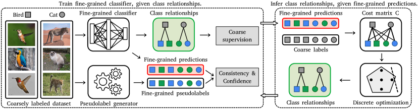
In this work, we propose FALCON (Fine grAined Labels from COarse supervisioN), a method that discovers fine-grained classes within a coarsely labeled dataset without any supervision. The key insight in FALCON is that fine-grained predictions can be combined with the relations between coarse and fine classes to recover coarse predictions. With this insight, FALCON develops a specialized optimization procedure that alternates between inferring unknown relations between the coarse and fine-grained classes and training a fine-grained classifier. Relationships between the coarse and fine-grained classes are inferred by solving a discrete optimization problem, while the fine-grained classifier is trained using coarse supervision and fine-grained pseudo-labels. Moreover, FALCON can be seamlessly adapted to leverage multiple datasets with incompatible coarse classes, relabeling all of them at the same fine-grained level.

We compare FALCON to alternative baselines on eight image classification datasets and a single-cell dataset from biology domain. Experimental results show that FALCON effectively discovers fine-grained classes without supervision and consistently outperforms baselines on both image and single-cell data. For instance, on the tieredImageNet dataset with $608$ fine-grained classes, FALCON outperforms baselines by $22\%$. Moreover, when trained with multiple datasets with different coarse classes, FALCON effectively reuses different annotation policies to improve its performance.

2 Related Work

Weakly-supervised classification. Coarse labels can be utilized as a form of weak supervision. Previous works (Ristin et al., 2015; Taherkhani et al., 2019; Hsieh et al., 2019) boost fine-grained classification performance by training on a mixture of coarse and fine labels. Robinson et al. (2020) build a theoretical framework for analyzing coarse labels as a form of weak supervision. However, all these methods are trained in a supervised manner with both coarse and fine supervision. In contrast, FALCON does not use any fine-grained supervision and assumes that only coarse labels are available during training.

Cross-granularity few-shot learning. Cross-granularity few-shot learning (Ni et al., 2022) considers a setting where a model is trained on a set of coarse classes and it needs to adapt to the fine-grained classes given only a few labeled examples. Wu et al. (2018) combines a non-parametric classifier with a deep feature extractor to learn fine-grained representation space. Bukchin et al. (2021) propose a contrastive learning objective that decreases the angle between the augmented views of the same input while increasing the angle to other samples from the same coarse class. Ni et al. (2022) models the generation of samples from coarse classes by representing the fine-grained subclasses with latent variables. Liu et al. (2019) considers a few-shot setup where relations between coarse and fine classes are known beforehand. Our setting differs from the few-shot learning setting since we do not assume to have any fine-grained labels available. Instead, our goal is to discover fine-grained classes.

Fine-grained image retrieval. Fine-grained image retrieval (Touvron et al., 2021) utilizes coarse supervision to learn fine-grained representations. The learned representations capture fine-grained correspondences between samples and enable retrieval of images at finer granularity. To solve this task, previous works (Xu et al., 2021; Touvron et al., 2021) combine self-supervised representation learning with parametric or non-parametric coarse classifiers. Alternatively, Feng & Patras (2023) extends the self-supervised objective by reweighting the samples according to the similarity in the feature space. Different from image retrieval, our goal is to discover the underlying fine-grained classes within the coarsely labeled data.

Deep clustering. Clustering is a decades-old machine learning problem (Lance & Williams, 1967). Recent deep clustering methods (Chang et al., 2017; Asano et al., 2020; Gadetsky & Brbić, 2023) outperform the classical approaches using deep neural networks trained with carefully designed optimization objectives. Common deep clustering objectives encourage consistent predictions for similar samples (Gansbeke et al., 2020), or gradually fit the network to the most confident predictions (Niu et al., 2022; Asano et al., 2020). Deep clustering methods can be used for the inference of fine-grained classes in an unsupervised manner; however, they typically result in a suboptimal performance due to the difficulty of the task. To address this limitation, we design a method that can effectively utilize available coarse-level supervision for the discovery of fine-level classes.

3 Fine-grained Class Discovery

Figure 1: FALCON simultaneously discovers fine-grained classes and infers relationships between the discovered fine and the available coarse classes by coarse supervision. The fine-grained classifier optimizes the loss (10), while the class relationships are inferred by solving a discrete optimization problem (14).

Problem setup. Let $\mathcal{X}$ be a sample space and $\mathcal{Y}_{C}$ a set of $K_{C}$ coarse classes. We assume a coarsely labeled dataset $\mathcal{D}=\{(\mathbf{x}^{i},y_{c}^{i})\}_{i=1}^{N}$ is given, where $\mathbf{x}^{i}\in\mathcal{X}$ and $y_{c}^{i}\in\mathcal{Y}_{C}$. Additionally, every sample $\mathbf{x}\in\mathcal{D}$ is associated with a fine-grained class $y_{\text{f}}$ from an unknown set of fine-grained classes $\mathcal{Y}_{F}$. We assume that every fine-grained class $y_{\text{f}}\in\mathcal{Y}_{F}$ is associated with a single coarse class $y_{c}\in\mathcal{Y}_{C}$, i.e., has a single coarse-grained parent. The number of fine classes $K_{F}=|\mathcal{Y}_{F}|$ is greater than $K_{C}$ and it is known beforehand or can be estimated. Given a coarsely labeled dataset $\mathcal{D}$, our goal is to discover a set of fine-grained classes $\mathcal{Y}_{F}$. Thus, we want to recover fine-grained labeling $\tau_{F}:\mathcal{X}\rightarrow\mathcal{Y}_{F}$ by using only supervision from the coarsely labeled dataset.

3.1 Parameterizing the Fine-grained Class Discovery

A key observation in FALCON is that the composition of fine-grained predictions and class relationships produces coarse predictions. Consequently, we can connect fine predictions and coarse labels using class relations.

We model the fine-grained labeling $\tau_{F}$ with a probabilistic classifier $f_{\theta}:\mathcal{X}\rightarrow\Delta^{K_{F}-1}$ that maps inputs into ($K_{F}-1$)-dimensional probabilistic simplex $\Delta^{K_{F}-1}$. Then, we can recover assignments of samples to fine-grained classes $\mathcal{Y}_{F}$ by taking the argmax over classifier’s fine-grained predictions $\mathbf{p}_{\text{f}}$:

$$\tau_{F}(\mathbf{x})=\text{argmax}_{i}\,\mathbf{p}_{\text{f}}^{i},\quad\text{where}\quad\mathbf{p}_{\text{f}}=f_{\theta}(\mathbf{x}).$$ (1)

Here, $\theta\in\mathbb{R}^{d}$ parameterizes the fine-grained classifier and $\mathbf{p}_{\text{f}}$ is a point on $\Delta^{K_{F}-1}$.

We obtain coarse predictions $\mathbf{p}_{\text{c}}$ using fine-grained predictions $\mathbf{p}_{\text{f}}$ and class relations $\mathbf{M}$:

$$\mathbf{p}_{\text{c}}=\mathbf{M}^{T}\mathbf{p}_{\text{f}},$$ (2)

where $\mathbf{p}_{\text{c}}$ is a point on ($K_{C}-1$)-dimensional probabilistic simplex $\Delta^{K_{C}-1}$ and $\mathbf{M}\in\{0,1\}^{K_{F}\times K_{C}}$ is a binary matrix of fine-coarse class relationships. In particular, element $\mathbf{M}_{ij}$ is $1$ if the i-th fine-grained class is associated with the j-th coarse class and $0$ otherwise. Since every fine-grained class is related to a single coarse class, every matrix row of $\mathbf{M}$ sums to $1$. Thus, $\mathbf{M}$ is the adjacency matrix of an undirected bipartite graph that models relationships between coarse and fine classes.

FALCON simultaneously learns the fine-grained classifier and class relationships by coarse supervision. We use the cross-entropy objective (CE) to leverage coarse supervision and learn parameters $\theta$ and relations $\mathbf{M}$:

$$\mathcal{L}_{\text{coarse}}(\theta,\mathbf{M}|\mathcal{D})=\frac{1}{|\mathcal{D}|}\sum_{(\mathbf{x},y_{c})\in\mathcal{D}}\text{CE}(\mathbf{M}^{T}f_{\theta}(\mathbf{x}),y_{c}).$$ (3)

Joint optimization of loss (3) w.r.t the discrete class relations $\mathbf{M}$ and continuous classifier parameters $\theta$ is unstable and computationally intensive, as we show in the following sections. To avoid these problems, we extend the objective (3) and conduct alternating optimization of parameters $\theta$ and class relationships $\mathbf{M}$.

The alternating optimization in FALCON is visualized in Figure 1 and proceeds as follows. We first train the fine-grained classifier parameterized by $\theta$, given class relationships $\mathbf{M}$. Next, we infer class relationships $\mathbf{M}$, given fine-grained predictions of the classifier and coarse labels. The procedure is repeated for a predefined number of epochs. The following sections describe the two steps of FALCON’s optimization procedure: (i) training the fine-grained classifier, and (ii) inferring class relationships. The technical details of the optimization are in Appendix A.

3.2 Training Fine-grained Classifier

With the class relationships $\mathbf{M}$ fixed, $\mathcal{L}_{\text{coarse}}(\theta,\mathbf{M}|\mathcal{D})$ becomes $\mathcal{L}_{\text{coarse}}(\theta|\mathbf{M},\mathcal{D})$. Training the fine-grained classifier by solely optimizing (3) with coarse labels is unable to separate fine-grained classes within a coarse class (see Appendix B for the detailed analysis). To overcome this issue, in FALCON we introduce additional objectives that encourage local consistency and confidence of fine-grained predictions, yielding better separation of fine-grained classes within a coarse class.

Consistent and confident fine-grained predictions. We enforce consistency in local fine-grained predictions by considering the nearest neighbors of a given input. We encourage consistent predictions by maximizing the dot product between the predictions for the input sample and the predictions for the neighbouring samples. The corresponding loss $\mathcal{L}_{\text{NN}}$ is a log-geometric mean of the dot products (Gansbeke et al., 2020):

$$\mathcal{L}_{\text{NN}}(\theta|\mathcal{D})=\frac{-1}{NL}\sum_{(\mathbf{x},y_{c})\in\mathcal{D}}\sum_{\hat{\mathbf{x}}\in\mathcal{N}(\mathbf{x},y_{c})}\ln(f_{\theta_{\text{EMA}}}(\hat{\mathbf{x}})^{T}f_{\theta}(\mathbf{x})),$$ (4)

where $\mathcal{N}(\mathbf{x},y_{c})$ denotes the set of nearest neighbours of a given sample $\mathbf{x}$ within the same coarse class $y_{c}$, $\hat{\mathbf{x}}$ is an element from $\mathcal{N}(\mathbf{x},y_{c})$, and $L=|\mathcal{N}(\mathbf{x},y_{c})|$. Parameters $\theta_{\text{EMA}}$ are computed as an exponential moving average of $\theta$ over iterations (Tarvainen & Valpola, 2017):

$$\theta_{\text{EMA}}^{t}=\gamma\theta_{\text{EMA}}^{t-1}+(1-\gamma)\theta^{t},$$ (5)

where $\gamma$ is a hyperparameter and $t$ represents training iterations. Different from (Gansbeke et al., 2020), we retrieve the nearest neighbors from the same coarse class and use EMA parameters.

The loss $\mathcal{L}_{\text{NN}}$ ensures consistent fine-grained predictions across the neighbouring samples. However, consistent predictions can also be ambiguous, which prevents the formation of adequate fine-grained classes. Hence, we encourage a more confident assignment of samples into fine-grained classes by minimizing the cross entropy between the fine-grained predictions and the target distribution $q$:

$$\mathcal{L}_{\text{conf}}(\theta|\mathbf{M},\mathcal{D})=\frac{1}{N}\sum_{(\mathbf{x},y_{c})\,\in\,\mathcal{D}}\text{CE}(q_{\theta_{\text{EMA}}}(\mathbf{x},y_{c}),f_{\theta}(\mathbf{x})).$$ (6)

The fine-grained target distribution $q$ utilizes information from the coarse label $y_{c}$ to sharpen the distribution over fine-grained classes. We define the target distribution $q$ using class relations $\mathbf{M}$ and parameters $\theta_{\text{EMA}}$ as follows:

$$q_{\theta_{\text{EMA}}}(\mathbf{x},y_{c}):=\begin{cases}\frac{\exp(\mathbf{s}^{y_{\text{f}}}/T)}{Z},&\text{if }\mathbf{M}_{y_{\text{f}},y_{c}}=1\\ 0,&\text{otherwise},\end{cases}$$ (7)

where $T$ is a scalar temperature hyperparameter and $\mathbf{s}$ denotes the logits of the fine-grained classifier. The scalar $Z$ is a normalization constant and is defined as $Z=\sum_{i=1}^{K_{F}}\mathbf{M}_{i,y_{c}}\exp(\mathbf{s}^{i}/T)$.

The introduced target distribution $q$ and the fine-grained predictions for nearest neighbours can be viewed as a form of pseudolabels, as visualized in Figure 1 (left).

We join the loss $\mathcal{L}_{\text{NN}}$ (4) and the loss $\mathcal{L}_{\text{conf}}$ (6) into a joint loss $\mathcal{L}_{\text{fine}}$ that operates over the fine-grained predictions:

$$\mathcal{L}_{\text{fine}}(\theta|\mathbf{M},\mathcal{D})=\mathcal{L}_{\text{NN}}(\theta|\mathcal{D})+\mathcal{L}_{\text{conf}}(\theta|\mathbf{M},\mathcal{D})$$ (8)

Regularization. To avoid degenerate solutions, we further stabilize the training by introducing the entropy maximization loss $\mathcal{L}_{\text{reg}}$ (9), which is commonly used in clustering-related tasks (Gansbeke et al., 2020; Cao et al., 2022).

$$\mathcal{L}_{\text{reg}}(\theta|\mathcal{D})=\ln K_{F}+\sum_{i=1}^{K_{F}}\overline{\mathbf{p}}_{\text{f}}^{i}\ln\overline{\mathbf{p}}_{\text{f}}^{i},\,\,\overline{\mathbf{p}}_{\text{f}}=\frac{1}{N}\sum_{\mathbf{x}\in\mathcal{D}}f_{\theta}(\mathbf{x}).$$ (9)

The loss $\mathcal{L}_{\text{reg}}$ helps to avoid degenerate solutions that assign all samples to the same fine class.

Total loss of the fine-grained classifier. Putting it all together, FALCON optimizes the following objective for training the fine-grained classifier:

$$\underset{\theta\,\in\,\mathbb{R}^{d}}{\text{min}}\left\{\mathcal{L}(\theta|\mathbf{M},\mathcal{D})=\lambda_{1}\mathcal{L}_{\text{coarse}}+\lambda_{2}\mathcal{L}_{\text{fine}}+\lambda_{3}\mathcal{L}_{\text{reg}}\right\},$$ (10)

where $\lambda_{1},\lambda_{2}$ and $\lambda_{3}$ are modulation hyperparameters. The importance of each loss component is ablated in Section 5.3. Using predictions of the fine-grained classifier, FALCON next learns relationships between fine and coarse classes.

3.3 Inferring Class Relationships

Given the fine-grained classifier $f_{\theta}$, optimizing (3) involves solving discrete optimization over all possible class relations to find the optimal $\mathbf{M}$. The main difficulties come from the fact that the objective (3) is both a nonlinear function of $\mathbf{M}$ and hard to evaluate due to the large dataset size $N$ ($K_{C}<K_{F}\ll N$). Yet, discrete optimization solvers require many evaluations of the objective function and are only effective for specific problem classes such as linear objective functions. To overcome the aforementioned issues, FALCON resorts to the approximation of the objective (3), leading to the efficient inference of the class relationships.

Approximated coarse-grained supervision. We begin by fixing parameters $\theta$ of the fine-grained classifier and rewriting loss over coarse labels $\mathcal{L}_{\text{coarse}}$ in the matrix form:

$$\mathcal{L}_{\text{coarse}}(\mathbf{M}|\theta,\mathcal{D})=-\frac{1}{N}\text{tr}(\mathbf{Y}_{oh}^{T}\ln(\mathbf{P}\mathbf{M})),$$ (11)

where $\mathbf{Y}_{oh}\in\{0,1\}^{N\times K_{C}}$ is a matrix that represents coarse labels as one-hot vectors and $\mathbf{P}\in[0,1]^{N\times K_{F}}$ is a matrix that gathers fine-grained predictions into rows. The logarithm is applied elementwise while $\text{tr}(\cdot)$ is the trace operator.

To overcome the discussed challenges, we approximate the loss $\mathcal{L}_{\text{coarse}}$ using Taylor expansion and reformulate it in a computationally efficient way:

$$\mathcal{L}_{\text{coarse}}^{\text{lin}}(\mathbf{M}|\theta,D)=-\frac{1}{N}\text{tr}(\mathbf{Y}_{oh}^{T}\mathbf{P}\mathbf{M}).$$ (12)

Details of the derivation are provided in Appendix C. The cost matrix $\mathbf{C}=\mathbf{Y}_{oh}^{T}\mathbf{P}\in\mathbb{R}^{K_{C}\times K_{F}}_{+}$ effectively encodes the strength of connections between coarse and fine classes. Each cost matrix element $\mathbf{C}_{ij}$ is proportional to the number of samples from coarse class $j$ assigned to the fine class $i$. Thus, the optimal solution of (12) preserves only the strongest connections between coarse and fine classes. Note that the objective (12) can be evaluated more efficiently than (11) since the matrix $\mathbf{Y}_{oh}^{T}\mathbf{P}$ can be precomputed.

Regularization. Computing the optimal solution for the objective $\mathcal{L}_{\text{coarse}}^{\text{lin}}$ may lead to severely imbalanced assignments of fine classes across coarse classes. Hence, we introduce an additional regularization term that penalizes the deviation from the balanced assignment of fine-grained classes across coarse classes:

$$\mathcal{L}_{\text{bal}}(\mathbf{M})=\frac{1}{K_{C}}\text{tr}(\mathbf{M}^{T}\boldsymbol{1}_{K_{F}}\boldsymbol{1}_{K_{F}}^{T}\mathbf{M})-\frac{K_{F}^{2}}{K_{C}^{2}},$$ (13)

where $\boldsymbol{1}_{K_{F}}$ denotes $K_{F}$-dimensional column vector of ones. Thus, $\mathbf{M}^{T}\boldsymbol{1}_{K_{F}}$ is a $K_{C}$-dimensional vector whose values correspond to the number of fine classes associated with every coarse class. The constant $K_{F}^{2}/K_{C}^{2}$ corrects the loss so that it yields zero in the case of the balanced assignment.

Total loss for inferring class relationships. FALCON recovers the relations between fine and coarse classes $\mathbf{M}$ by solving the following optimization problem:

$$\underset{\mathbf{M}\,\in\,\mathcal{M}}{\text{min}}\left\{\mathcal{L}(\mathbf{M}|\theta,\mathcal{D})=\mathcal{L}_{\text{coarse}}^{\text{lin}}(\mathbf{M}|\theta,D)+\lambda_{M}\mathcal{L}_{\text{bal}}(\mathbf{M})\right\},$$ (14)

where $\lambda_{M}$ is a hyperparameter that controls the influence of $\mathcal{L}_{\text{bal}}$. The set $\mathcal{M}$ contains all possible class relations:

$$\mathcal{M}=\{ \mathbf{M}\in\{0,1\}^{K_{F}\times K_{C}}\,|\,$$

$$\mathbf{M}\boldsymbol{1}_{K_{C}}=\boldsymbol{1}_{K_{F}},\mathbf{M}^{T}\boldsymbol{1}_{K_{F}}\geq\boldsymbol{1}_{K_{C}}\}.$$ (15)

The optimization problem (14) is essentially an integer quadratic program with linear constraints (as discussed in Appendix D). The problem involves the optimization of only $K_{F}\cdot K_{C}$ binary variables. Thus, we can swiftly compute the solution of (14) using modern hardware, even though the resulting problem is inherently NP-hard (Fotakis et al., 2021). Our experiments suggest that FALCON can be applied to real-world datasets with hundreds of fine-grained classes.

3.4 Training on Multiple Datasets

Fine-grained classes can be grouped into coarse classes in different ways. For example, one can group animals according to diet (carnivores vs omnivores), size (small vs large), or biological taxonomy (Canis lupus vs Canis familiaris). Thus, datasets often have different labels despite aggregating the instances of the same fine classes (Bevandić et al., 2024). FALCON is seamlessly applicable to training on multiple datasets with different coarse labels.

Specifically, let $\mathcal{D}_{l}=\{(\mathbf{x}^{i},y_{c}^{i})\}_{i=1}^{N_{l}}$ be a dataset where $\mathbf{x}^{i}\in\mathcal{X}$, $y_{c}^{i}\in\mathcal{Y}_{C}^{l}$, and $\mathcal{Y}_{C}^{l}$ is dataset-specific set of coarse classes. We assume that samples from every dataset $\mathcal{D}_{l}$ can be associated with fine classes from a shared set of fine classes $\mathcal{Y}_{F}$. We aggregate samples from $D$ datasets into a combined dataset $\mathcal{D}_{\text{all}}$:

$$\mathcal{D}_{\text{all}}=\cup_{l=1}^{D}\{(\mathbf{x},y,l)\,|\,(\mathbf{x},y)\in\mathcal{D}_{l}\}.$$ (16)

Every datapoint in $\mathcal{D}_{\text{all}}$ is a triplet of input, coarse label, and index of the dataset from which the sample originates.

We extend the parametrization (3) by modeling $D$ dataset-specific mappings $\mathbf{M}_{l}$:

$$\mathcal{L}_{\text{coarse}}(\theta,\mathbf{M}_{1},\dots,\mathbf{M}_{D}|\mathcal{D}_{\text{all}})=\\ \frac{1}{|\mathcal{D}_{\text{all}}|}\sum_{(\mathbf{x},y_{c},l)\in\mathcal{D}_{\text{all}}}\text{CE}(\mathbf{M}_{l}^{T}f_{\theta}(\mathbf{x}),y_{c}).$$ (17)

Thus, integrating multiple datasets into the FALCON framework only requires inferring $D$ dataset-specific class relations $M_{l}$. As in the case of a single dataset, FALCON infers dataset-specific class relations by solving (14). All $D$ discrete optimization problems are mutually independent and can be solved in parallel.

The fine-grained classifier optimizes the same losses described in Section 3.2. Still, dataset-specific coarse supervision results in different gradient updates for the same set of fine-grained predictions, resulting in better fine-grained performance, as we show in the experiments. Technical details for the multi-dataset training procedure are in Appendix E.

4 Experimental Setup

4.1 Datasets & Metrics

Datasets. We evaluate FALCON on eight image classification datasets including Living17, Nonliving26, Entity30, Entity13, tieredImageNet (Ren et al., 2018), CIFAR100 (Krizhevsky, 2009), CIFAR-SI, and CIFAR68 datasets. Datasets Living17, Nonliving26, Entity30 and Entity13 are from the BREEDS benchmark (Santurkar et al., 2021). For the tieredImageNet dataset(Ren et al., 2018), we joined training, validation and test taxonomies into a single dataset with $608$ fine classes assigned across $34$ coarse classes. For the CIFAR100 dataset, we used the original labels with $20$ coarse and $100$ fine classes. The original CIFAR100 dataset has an equal number of fine classes associated with every coarse class and an equal number of samples in every fine class. Hence, we additionally introduce two unbalanced versions of the CIFAR100 dataset that we name CIFAR68 and CIFAR-SI datasets. In the case of CIFAR68 dataset, we remove $32$ fine classes from the original dataset to disbalance the number of fine classes in coarse classes. In the case of CIFAR-SI dataset, we remove up to $70\%$ of samples from every fine class, which effectively disbalances sample distribution. We evaluate performance on the image datasets in the inductive setting on the predefined train/test splits.

In addition, to show that FALCON is widely applicable we consider a single-cell RNA-seq dataset from the biology domain. We evaluate FALCON on the PBMC dataset gathered from blood samples of COVID-19 patients (Lindeboom et al., 2023). The task is to classify cells into fine-grained cell subtypes given coarse-grained cell types. We evaluate the method on the ground-truth cell subtypes that correspond to fine-grained labels. The PBMC dataset is highly imbalanced (Gini coefficient greater than 0.5). We evaluate performance on the single-cell data in the transductive setting.

The overview of all considered datasets is shown in Table 1. Abbreviation L17 stands for Living17, N26 for Nonliving26, E30 for Entity30, E13 for Entity13, C100 for CIFAR100, C68 for CIFAR68, CSI for CIFAR Sample Imbalanced, tIN for tieredImageNet, and PB for PBMC. More details about the datasets are provided in Appendix F.

Table 1: Overview of nine evaluation datasets. The four rows correspond to the dataset abbreviation, the number of coarse classes, the number of fine classes, and the input resolution.

Dataset	L17	N26	E30	E13	C100	C68	CSI	tIN	PB
# Coarse	17	26	30	13	20	20	20	34	27
# Fine	68	104	240	260	100	68	100	608	83
Res.	$224^{2}$	$224^{2}$	$224^{2}$	$224^{2}$	$32^{2}$	$32^{2}$	$32^{2}$	$224^{2}$	2k

Metrics. We train FALCON and baselines without access to fine-grained ground-truth labels. Thus, we report fine-grained clustering accuracy (Gansbeke et al., 2020; Vaze et al., 2022) as an evaluation metric:

$$\text{Acc}=\underset{p\in\mathcal{P}(\mathcal{Y}_{\text{f}})}{\max}\frac{1}{|D|}\sum_{i=1}^{|D|}\,\llbracket y_{\text{f}}^{i}=p(\hat{y}^{i}_{\text{f}})\rrbracket.$$ (18)

Here, $\mathcal{P}(\mathcal{Y}_{\text{f}})$ is a set of all permutations of fine class labels. In practice, the metric can be efficiently computed using Hungarian algorithm (Kuhn, 1955). Additionally, we report adjusted rand index (ARI). Since FALCON also learns class relations, we report the difference between learned label relations and the ground-truth graph using the graph edit distance (GED) (Fischer et al., 2017). The graph edit distance counts the number of nodes and edges that have to be added or removed in order to match the target graph.

4.2 Baselines

Since there is no method specifically design for the setting of fine-grained class discovery with coarse supervision, we compare FALCON with methods that could be applied in this setting, including clustering and cross-granularity few-shot methods that we adapt for fine-grained class discovery.

SCAN (Gansbeke et al., 2020) is a deep clustering method which we directly apply for fine-grained class discovery by clustering the data. However, SCAN cannot utilize information about coarse classes during the training. Thus, we additionally adapt SCAN by enforcing consistent predictions across neighbors retrieved within the same coarse class. This adaptation enables SCAN to utilize coarse supervision. We call this baseline SCAN-C.

We further include cross-granularity few-shot learning methods as baselines. ANCOR (Bukchin et al., 2021) is a cross-granularity few-shot method which learns fine-grained representation space. Thus, we run K-Means over the extracted features to recover the fine-grained predictions. We use the same approach to adapt SNCA (Wu et al., 2018). SCGM (Ni et al., 2022) is a few-shot method which can be directly applied to fine-grained class discovery since it provides fine-grained predictions.

We also include GEORGE (Sohoni et al., 2020) which conducts distributionally robust optimization of the coarse classification objective. GEORGE only learns fine-grained representation space so we again run the K-Means algorithm to recover the fine-grained predictions.

Finally, we can determine the upper bound of the performance by empirical risk minimization (ERM) (Vapnik, 1998) over fine-grained labels.

4.3 Implementation Details

We use ResNet18 (He et al., 2016) as the backbone for small images from the CIFAR dataset and ResNet50 as the backbone for large images from the remaining five image datasets. We initialize all methods (i.e., FALCON and all baselines) with self-supervised pretraining method MoCoV3 (Chen et al., 2021). We update all parameters of the model during the training. We pair weak augmentations of the input with $\theta_{\text{EMA}}$ and strong augmentations with $\theta$, as in (Chen et al., 2021). We retrieve nearest neighbours using the distances between self-supervised feature representations. Hyperparameter search was conducted on the CIFAR100 dataset using the TPE algorithm implemented in Optuna (Akiba et al., 2019). We solve the discrete optimization problem using Gurobi (Gurobi Optimization, LLC, 2023).

In the case of single-cell data, we use randomly initialized MLP with 4 linear layers and ReLU activations. We retrieve the nearest neighbours by computing the distance over the top 2k highly variable genes. More implementation details are in the Appendix G. Our code is publicly available.

5 Experimental Evaluation

Table 2: Fine-grained accuracy (Acc) and adjusted rand index (ARI) on eight image datasets and a single-cell RNA-seq dataset. Results are averaged over three runs. Transductive evaluation is denoted with $\dagger$.

Method	Living17		NLiving26		Entity30		Entity13		CIFAR100		CIFAR68		CIFAR-SI		tieredIN		$\text{PBMC}^{\dagger}$
	Acc	ARI	Acc	ARI	Acc	ARI	Acc	ARI	Acc	ARI	Acc	ARI	Acc	ARI	Acc	ARI	Acc	ARI
Up. Bound	86.3	76.1	84.6	73.8	85.6	74.5	85.9	75.4	74.5	57.0	78.8	62.9	73.0	56.6	79.1	65.1	88.9	86.4
SCAN	61.9	50.1	54.3	39.7	51.1	38.4	50.8	37.5	47.1	34.4	51.4	39.8	47.4	35.8	43.6	28.9	20.7	13.5
ANCOR	27.7	36.1	27.9	34.7	17.0	20.2	8.4	8.5	23.4	26.6	30.1	33.7	28.7	25.9	47.8	34.1	44.9	37.7
SNCA	39.2	30.9	43.6	31.1	36.1	23.4	35.1	20.9	42.9	18.9	47.6	23.3	41.3	21.6	22.3	11.0	29.5	20.2
GEORGE	62.8	53.2	58.8	47.2	50.1	35.6	49.6	35.7	51.9	36.0	59.6	42.8	51.2	36.7	43.0	29.1	37.7	32.4
SCGM	62.3	49.3	56.4	42.0	56.0	41.4	54.8	40.8	47.9	32.2	49.6	34.7	46.3	31.8	46.6	32.0	22.7	13.8
SCAN-C	67.1	54.7	60.4	45.8	60.6	46.2	57.7	43.7	48.7	36.1	54.3	41.9	48.6	38.0	48.2	33.2	20.3	13.2
FALCON	71.8	60.3	65.7	55.5	65.1	53.3	63.6	51.9	59.6	42.5	60.4	47.0	55.6	39.1	53.4	41.6	75.8	74.0

5.1 Quantitative Results

Fine-grained class discovery. We compare FALCON to alternative baselines on eight image classification datasets and a single-cell dataset. The results in Table 2 show that FALCON outperforms baselines by a large margin on both image and single-cell data. For example, on the BREEDS benchmark of four datasets (Living17, Nonliving26, Entity30, Entity13) FALCON achieves an average improvement of $9\%$ in terms of accuracy and $16\%$ in terms of ARI over the best baselines. On the tieredImageNet dataset with $608$ fine-grained classes grouped into $34$ coarse classes, FALCON outperforms the best baseline ANCOR by $12\%$ and $22\%$ in terms of accuracy and ARI, respectively. Moreover, improvements of FALCON can be observed on both balanced (BREEDS benchmark and CIFAR100), as well as unbalanced datasets (CIFAR68, CIFAR-SI, tieredImageNet and single-cell PBMC).

Evaluation of learned class relationships. FALCON infers the mapping between fine-grained and coarse-grained classes. We next evaluate how well the inferred coarse-fine class relationships agree with the ground truth relationships using the graph edit distance (GED). The graph edit distance of zero indicates that two graphs are the same and the ground truth relationships are perfectly inferred. We compare FALCON with SCGM which learns class relations implicitly through a data generation process. The results shown in Table 3 demonstrate that FALCON can perfectly match the ground truth relations for all balanced datasets which is not the case for the SCGM. For the imbalanced datasets, not all class relationships are correctly recovered but FALCON still substantially outperforms SCGM on all datasets. The discrepancy between the learned and the ground-truth relations comes from the fact that (14) finds the optimal solution given a classifier $f_{\theta}$. Thus, the obtained solution may differ from the true optimal solution. This discrepancy could be mitigated by employing a stronger classifier (Radford et al., 2021).

Table 3: Graph edit distance (GED) between the learnt class relations and the true class relations averaged over three runs.

GED$\downarrow$	L17	N26	E30	E13	C100	C68	CSI	tIN	PM
SCGM	30.7	74.7	98.7	45.3	61.3	57.0	61.3	132.0	88.7
FALCON	0.0	0.0	0.0	0.0	0.0	40.3	0.0	110.7	73.3

Training on multiple datasets. FALCON can learn from multiple datasets labeled with different coarse-level classes (Section 3.4). We evaluate the effectiveness of FALCON on the CIFAR100 dataset. The CIFAR100 dataset has a default grouping of $100$ fine classes into $20$ coarse classes which we denote with T1. We construct a meaningful alternative grouping of fine classes into coarse classes, which we denote as T2. For example, the default grouping T1 arbitrarily divides $10$ fine-grained vehicle classes into two coarse classes named Vehicles1 and Vehicles2. On the contrary, our alternative taxonomy groups fine-grained vehicle classes into Personal Vehicles and Transit Vehicles (see Appendix I for the full list of coarse classes in each taxonomy). We split the training set into two halves and label the first half according to T1 and the second half according to T2. Thus, the resulting splits, denoted with $\mathcal{D}_{1}$ and $\mathcal{D}_{2}$, correspond to two datasets with the same underlying set of fine-grained classes and different coarse classes. We keep the CIFAR100 test set unmodified to track the generalization performance for different training configurations.

Table 4 shows the results of using FALCON to simultaneously learn from two coarsely labeled datasets with different labeling policies. The top two rows show fine-grained accuracy and ARI after training FALCON on $\mathcal{D}_{1}$ or $\mathcal{D}_{2}$. Compared to FALCON trained on a single dataset, we observe $14\%$ relative improvement according to ARI and $10\%$ relative improvement according to clustering accuracy. These results indicate that FALCON can effectively utilize different labeling policies to improve performance.

To evaluate the benefits of training from multiple datasets using baseline methods, we train SCAN-C on the same datasets. While SCAN-C can simultaneously learn from multiple datasets, the gains from different labelings are marginal compared to FALCON (2% improvement in terms of ARI).

Table 4: FALCON benefits from simultaneous training on multiple datasets with incompatible coarse labels.

Train DS	Samples	Taxonomy	SCAN-C		FALCON
			Acc	ARI	Acc	ARI
$\mathcal{D}_{1}$	N/2	T1	48.7	35.9	56.0	38.6
$\mathcal{D}_{2}$	N/2	T2	47.8	34.4	56.6	38.7
$\mathcal{D}_{\text{all}}$	N	T1&T2	49.6	36.7	61.5	43.9

Aggregating multiple training datasets implicitly increases the number of training samples and thus improves the generalization. Hence, we analyze the influence of different labeling policies in isolation by repeating the experiment with an equal number of samples in each training dataset from Table 4. The results, summarized in Appendix J, confirm that FALCON can effectively utilize the different labeling policies. For example, FALCON trained on taxonomies T1&T2 improves 7% in terms of accuracy over the FALCON trained only on T2. Contrary, SCAN-C trained on T1&T2 improves only 1% over the SCAN-C trained only on T2. Altogether, these results indicate that FALCON can effectively learn from multiple datasets labeled with different labeling policies.

5.2 Qualitative Results

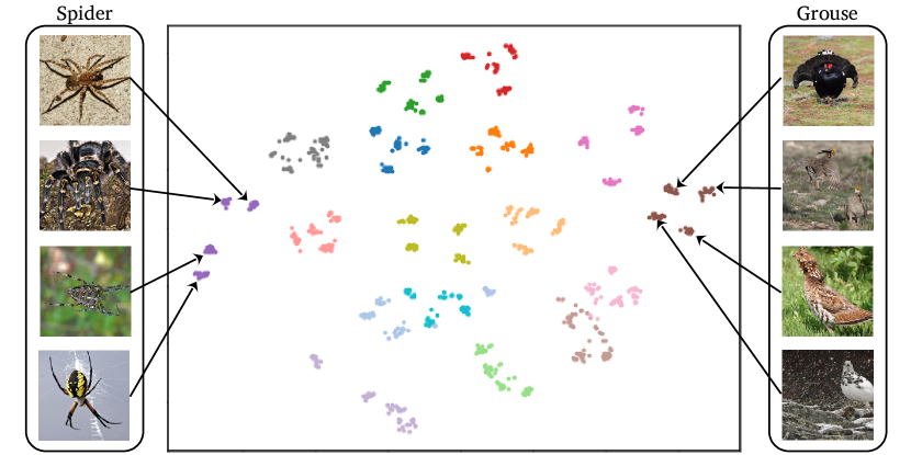
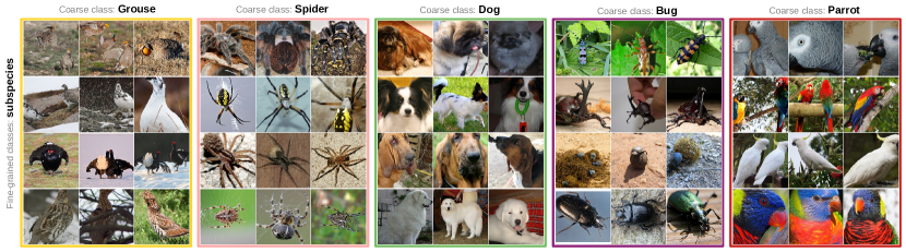
We next visually inspect the quality of the embedding space learnt by FALCON. Figure 2 shows two-dimensional t-SNE plot (Hinton & Roweis, 2002) of the embedding space learnt by FALCON on the Living17 dataset. The results show that samples assigned to the same coarse-grained classes are separated into multiple fine-grained classes.

To validate that these fine classes are correct and represent different subspecies of animals, we look into representative examples from every fine-grained class and confirm that the examples indeed reflect different subcategories. For example, the four fine classes of coarse class Spider correspond to subspecies of spiders including Barn spider, Tarantula, Garden spider, and Black and gold spider. Similarly, the inferred fine-grained classes of Grouse correspond to Black grouse, Prairie grouse, Ruffed grouse and Ptarmigan. This indicates that the embedding space learnt by FALCON indeed reflects fine-grained representations.

Figure 2: The t-SNE plot of Living17 test samples in the embedding space learned by FALCON. Coarse-grained classes used to supervise the model are shown in different colors. The images at the left and right side show representative examples of inferred fine-grained classes for coarse classes Spider and Grouse.

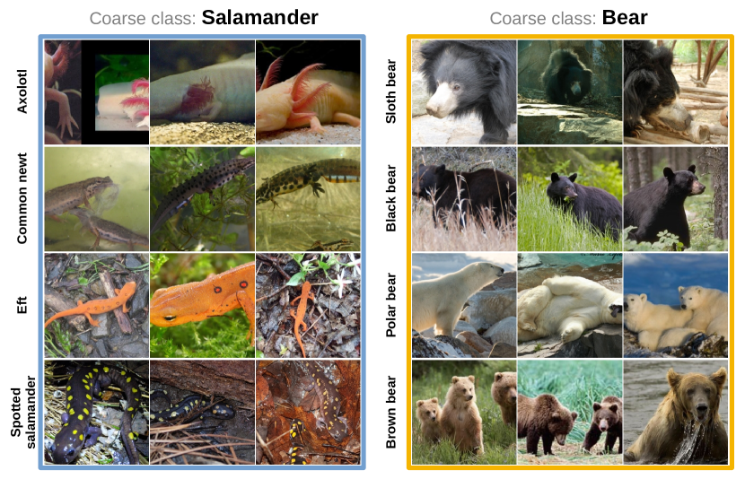
We next visualize the three most confident predictions for different fine-grained classes. Figure 3 shows the three most confident samples for every fine-grained class associated with coarse classes Salamander and Bear from the Living17 dataset. We validate the recovered fine-grained classes and confirm that they indeed correspond to different salamander subspecies (Axolotl, Common newt, Eft, and Spotted salamander) and bear subspecies (Sloth bear, Black bear, Polar bear, and Brown bear). This indicates that FALCON produces meaningful fine-grained classes even when differences between these subclasses are very subtle. We show more examples in the Appendix K.

Figure 3: Three most confident predictions for fine-grained classes associated with coarse class Salamander and Bear.

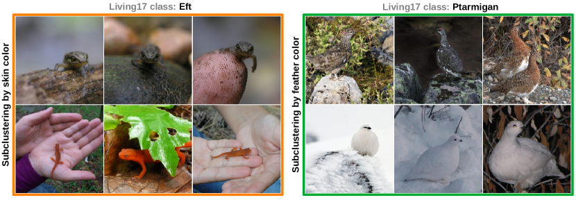
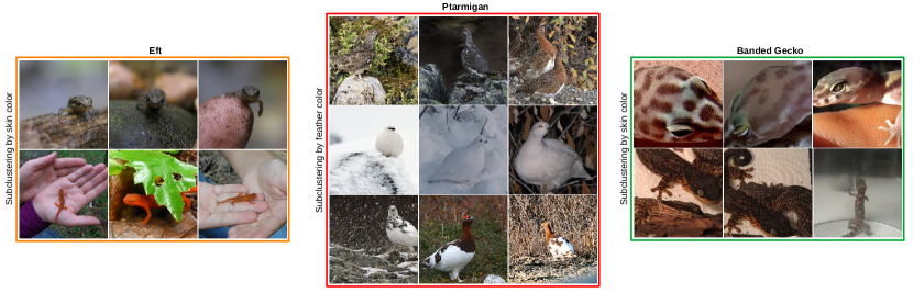
FALCON can also discover subclasses within existing fine-grained classes. To showcase this, we set 68 fine classes of the Living17 dataset as coarse classes and increased the expected number of fine-grained classes. Figure 4 shows the two subclasses discovered within classes Eft and Ptarmigan. The newly discovered subclasses differ by skin and feather color. Unfortunately, this evaluation can only be qualitatively verified since the appropriate ground-truth is unavailable. More visual examples can be found in Appendix L.

Figure 4: Subclasses discovered within fine-grained classes Eft and Ptarmigan. The discovered subclasses differ according to the skin (Eft) or feather (Ptarmigan) color.

5.3 Ablation Studies

Components of the objective. We next conduct ablation studies on the classifier’s objective function (10) which consists of coarse supervision $\mathcal{L}_{\text{coarse}}$, fine-grained consistency and confidence $\mathcal{L}_{\text{fine}}$, and entropy regularization $\mathcal{L}_{\text{reg}}$. To investigate the importance of each part, we modify FALCON by removing each loss component and then measure fine-grained clustering accuracy and ARI. We show the results on the CIFAR100 dataset in Table 5. Removing $\mathcal{L}_{\text{fine}}$ results in divergent fine-grained predictions for similar samples. Thus, the samples are arbitrarily grouped into subclasses and we observe poor fine-grained performance. Removing $\mathcal{L}_{\text{reg}}$ results in a skewed distribution of samples across fine-grained classes and poor fine-grained performance. Removing $\mathcal{L}_{\text{coarse}}$ eliminates coarse-level supervision and prevents joint learning of class relationships. Thus we also have to remove $\mathcal{L}_{\text{conf}}$ since it relies on class relations. Again, we observe a notable performance drop. This ablation confirms that all three losses contribute to strong fine-grained performance.

Table 5: Ablation study of the components from the objective function (10) on the CIFAR100 dataset. We report fine-grained performance averaged over three runs by removing different components of the FALCON objective.

$\mathcal{L}_{\text{coarse}}$	$\mathcal{L}_{\text{fine}}$	$\mathcal{L}_{\text{reg}}$	Acc	ARI
✓	✗	✓	22.9	14.6
✓	✓	✗	18.7	22.8
✗	✓	✓	51.0	32.0
✓	✓	✓	59.6	42.5

Estimated number of fine-grained classes. FALCON takes the expected number of fine-grained classes as a hyperparameter. However, in practice, we often do not know the number of classes in advance. In such a case, we can first estimate the number of novel classes. We estimate the number of classes as proposed in (Wang et al., 2018) and obtain $89$ for the CIFAR100 dataset and $76$ for the CIFAR68 dataset. We then train FALCON with the estimated number of fine-grained classes $K_{F}$. The results are shown in Table 6.

Remarkably, on the CIFAR100 dataset, FALCON with the estimated number of classes outperforms all other baselines trained with the ground truth number of fine classes. On the CIFAR68 dataset, FALCON outperforms all baselines except GEORGE which attains slightly better accuracy. FALCON’s sensitivity on different values of $K_{F}$ can be found in Appendix M.

Table 6: FALCON performance with the estimated number of fine-grained classes.

Method	CIFAR100		CIFAR68
	Acc	ARI	Acc	ARI
GEORGE	51.9	36.0	59.6	42.8
FALCON	59.6	42.5	60.4	47.0
FALCON-$\hat{K_{F}}$	54.9	39.9	59.1	45.7

Additional ablation studies. We validate the fine-grained performance for different hyperparameter values on CIFAR100. We validate $\lambda_{M}$ from (14), temperature $T$ from (7), and three loss modulation hyperparameters $\lambda_{1},\lambda_{2}$ and $\lambda_{3}$ from (10). The results are summarized in Appendix N. FALCON is robust to different values of hyperparameters. In addition, we evaluate the performance of FALCON with ground truth class relations in Appendix O. The results indicate that estimating class relations does not significantly affect the fine-grained classification performance. Thus, knowing class relations beforehand is not mandatory for good fine-grained performance.

6 Conclusion

We presented FALCON, a method that discovers fine-grained classes within coarsely labeled data. FALCON can simultaneously learn fine-grained classifier and relationships between the discovered fine and the available coarse classes by coarse supervision. We combine the coarse classification loss with additional fine-grained consistency and regularization losses to discover meaningful fine-grained classes. Simultaneously, we infer relations between the discovered fine and the available coarse classes by solving a discrete optimization problem. Such modular design enables FALCON to simultaneously train on multiple datasets with different coarse labels. FALCON consistently outperforms all baselines on large-scale image classification datasets and a single-cell dataset from the biology domain.

7 Limitations

Number of fine-grained classes. FALCON assumes that the number of fine-grained classes is known a priori, which is a common assumption in clustering and open-world learning problems (Gansbeke et al., 2020; Vaze et al., 2022; Cao et al., 2022; Gadetsky & Brbić, 2023). Still, FALCON can be combined with the existing methods which estimate this quantity (Wang et al., 2018) and deliver competitive results, as show in Section 5.3. Furthermore, FALCON is robust to noisy estimates of $K_{F}$, as discussed in Appendix M.

Consistently labeled dataset. FALCON assumes that samples within the same dataset are consistently labeled. That is, instances of the same fine-grained classes are always labeled as the same coarse class. However, FALCON can be simultaneously trained on multiple datasets with inconsistent labeling policies, as shown in Section 5.1. Thus, instances of the same fine-grained class can be differently labeled in different datasets.

The datasets are not severely imbalanced. The introduced entropy regularization term in FALCON encourages uniform distribution or samples to fine-grained classes. Since the influence of regularization is controlled by a hyperparameter, FALCON is still applicable even on sample-imbalanced datasets as we show in our experiments. However, extremely long-tailed class distribution will require replacing entropy regularization with alternative regularization objectives such as KL divergence between empirical label distribution and prior over the target label distribution.

Impact Statement

This paper presents work whose goal is to advance the field of Machine Learning. There are many potential societal consequences of our work, non which we feel must be specifically highlighted here.

Appendix A FALCON Training Algorithm

Algorithm A1 shows the training procedure for simultaneous learning of a fine-grained classifier and class relationships. We initialize feature extractor with self-supervised pretraining (Chen et al., 2021) in the case of images and randomly in the case of single-cell data. We construct a fine-grained classifier by appending a linear classifier atop the feature extractor. We initialize $\mathbf{M}$ by solving (14) for a randomly initialized cost matrix. In every epoch, we iteratively update parameters $\theta$ using SGD over the sampled minibatch. After every P iterations, we update class relations $\mathbf{M}$ using the current values of $\theta$. We do not gather predictions for the whole dataset but rather for a large enough subset (i.e. $20\times$ batch size). The training of $\theta$ then progresses with the new value of $\mathbf{M}$. Steps of the algorithm are outlined in Algorithm 1.

Algorithm A1 FALCON training on a single dataset

  Input: Fine-grained classifier $f_{\theta}$, dataset $\mathcal{D}$, number of fine-grained classes $K_{F}$, hyperparameters $\boldsymbol{\lambda},T,\lambda_{M}$, $\Omega$

  $\theta=\text{selfsup\_initialization}(\mathcal{D})$

  $\mathbf{M}$ = solve (14) for random cost matrix

  for $i=1$ to max_epochs do

     for $j=1$ to max_iters do

        Sample minibatch $(\mathbf{x},y)$ from $\mathcal{D}$

        $L_{\text{cls}}$ = evaluate loss (3)

        $L_{\text{cons}}$ = evaluate loss (8)

        $L_{\text{reg}}$ = evaluate loss (9)

        $L=\lambda_{1}\cdot L_{\text{cls}}+\lambda_{2}\cdot L_{\text{cons}}+\lambda_{3}\cdot L_{\text{reg}}$

        $\theta=\text{SGD}(L,\theta)$

        if j % $P$ = 0  then

           Gather $\mathbf{Y}_{oh}$ and $\mathbf{P}$ using $f_{\theta}$ over a subset of $\mathcal{D}$

           $\mathbf{C}=\mathbf{Y}_{oh}^{T}\mathbf{P}$

           $\mathbf{M}$ = solve (14) for cost matrix $\mathbf{C}$

        end if

     end for

  end for

  Output: classifier parameters $\theta$, class relationships $\mathbf{M}$

Appendix B Impact of Coarse Supervision to Fine-grained Predictions

Let $\mathbf{p}_{\text{f}}\in\Delta^{K_{F}-1}$ be the output of the fine-grained classifier $f_{\theta}$ for a given training example $\mathbf{x}$, $\mathbf{p}_{\text{c}}\in\Delta^{K_{C}-1}$ be the output of coarse-grained classifier $\mathbf{M}^{T}f_{\theta}$, and $j$ be the corresponding ground-truth coarse label. The loss $\mathcal{L}_{\text{coarse}}$ (3) for a particular sample can be written as:

$$\mathcal{L}_{\text{coarse}}(\theta|\mathbf{M},\mathbf{x},y_{c}=j)=\text{CE}(\mathbf{p}_{\text{c}},j),\quad\text{where}\quad\mathbf{p}_{\text{c}}=\mathbf{M}^{T}\mathbf{p}_{\text{f}}\quad\text{and}\quad\mathbf{p}_{\text{f}}=f_{\theta}(\mathbf{x}).$$ (19)

The gradient of $\mathcal{L}_{\text{coarse}}$ w.r.t $i$-th fine prediction equals to:

$$\frac{\partial\mathcal{L}_{\text{coarse}}}{\partial\mathbf{p}_{\text{f}}^{i}}=\frac{\partial\mathcal{L}_{\text{coarse}}}{\partial\mathbf{p}_{\text{c}}^{j}}\frac{\partial\mathbf{p}_{\text{c}}^{j}}{\partial\mathbf{p}_{\text{f}}^{i}}=\frac{\partial\mathcal{L}_{\text{coarse}}}{\partial\mathbf{p}_{\text{c}}^{j}}\mathbf{M}_{ij}.$$ (20)

Since $M$ is a binary matrix, the gradient of loss w.r.t $i$-th fine class boils down to:

$$\frac{\partial\mathcal{L}_{\text{coarse}}}{\partial\mathbf{p}_{\text{f}}^{i}}=\begin{cases}\frac{\partial\mathcal{L}_{\text{coarse}}}{\partial\mathbf{p}_{\text{c}}^{j}},&\text{if }\mathbf{M}_{ij}=1\\ 0,&\text{otherwise}\end{cases}$$ (21)

Thus, all fine-grained classes associated with coarse label $j$ receive the same gradient. Consequently, $\mathcal{L}_{\text{coarse}}$ only separates fine-grained classes that are associated with different coarse classes. We combine the coarse classification loss with additional fine-grained losses that further encourage the separation of fine classes.

Appendix C Step-by-step derivation of $\mathcal{L}^{\text{lin}}_{\text{cls}}$

We start from the cross entropy loss in the matrix form:

$$\mathcal{L}_{\text{coarse}}(\mathbf{M}|\theta,D)=-\frac{1}{N}\text{tr}(\mathbf{Y}_{oh}^{T}\ln(\mathbf{P}\mathbf{M})).$$ (22)

The logarithm function can be expressed with the Taylor series for $0<x\leq 2$ as:

$$\ln x=\sum_{i=1}^{\infty}\frac{(-1)^{i+1}}{i}(x-1)^{i}.$$ (23)

All row vectors of matrix $\mathbf{P}$ are points on $\Delta^{K_{F}-1}$ and all entries of $\mathbf{M}$ are either 0 or 1 therefore elements of $\mathbf{P}\mathbf{M}$ are positive and less or equal to 1. Consequently, we can approximate the logarithm function with the Taylor series truncated after the first term.

$$\mathcal{L}_{\text{coarse}}(M|\theta,D) =-\frac{1}{N}\text{tr}(\mathbf{Y}_{oh}^{T}\ln(\mathbf{P}\mathbf{M}))$$ (24)

$$\approx-\frac{1}{N}\text{tr}(\mathbf{Y}_{oh}^{T}(\mathbf{P}\mathbf{M}-\boldsymbol{1}_{N\times K_{C}}))$$ (25)

$$=-\frac{1}{N}\text{tr}(\mathbf{Y}_{oh}^{T}\mathbf{P}\mathbf{M}-\mathbf{Y}_{oh}^{T}\boldsymbol{1}_{N\times K_{C}})$$ (26)

$$=-\frac{1}{N}\text{tr}(\mathbf{Y}_{oh}^{T}\mathbf{P}\mathbf{M})+\frac{1}{N}\text{tr}(\mathbf{Y}_{oh}^{T}\boldsymbol{1}_{N\times K_{C}})$$ (27)

$$=-\frac{1}{N}\text{tr}(\mathbf{Y}_{oh}^{T}\mathbf{P}\mathbf{M})+1$$ (28)

$$\cong-\frac{1}{N}\text{tr}(\mathbf{Y}_{oh}^{T}\mathbf{P}\mathbf{M})$$ (29)

Appendix D Class Relationships by Solving Integer Quadratic Program

Integer quadratic programs (Boyd & Vandenberghe, 2014) are programs of the following form:

$$\underset{\mathbf{x}}{\text{min}}\quad\mathbf{x}^{T}A_{0}\mathbf{x}+\mathbf{b}_{0}^{T}\mathbf{x}+c_{0}$$ (30)

subjected to inequality and equality constraints:

$$\mathbf{b}_{i}^{T}\mathbf{x}+c_{i}\leq 0,\quad i=1,\dots,m$$ (31)

$$\mathbf{d}_{j}\mathbf{x}+e_{j}=0,\quad j=1,\dots,n.$$ (32)

The matrix $A$ is symmetric positive semidefinite, all $\mathbf{b}_{j}$, all $\mathbf{d}_{j}$ are real vectors, and $c_{i}$ and $e_{j}$ are real scalars. The variable $\mathbf{x}$ is restricted to take only integer values.

Our optimization problem for finding class relationships (14) equals to:

$$\underset{\mathbf{M}\in\mathcal{M}}{\text{min}}\quad-\frac{1}{N}\text{tr}(\mathbf{Y}_{oh}^{T}\mathbf{P}\mathbf{M})+\lambda_{M}\left(\frac{1}{K_{C}}\text{tr}(\mathbf{M}^{T}\boldsymbol{1}_{K_{F}}\boldsymbol{1}_{K_{F}}^{T}\mathbf{M})-\frac{K_{F}^{2}}{K_{C}^{2}}\right)$$ (33)

with

$$\mathcal{M}=\{\mathbf{M}\in\{0,1\}^{K_{F}\times K_{C}}\,|\,\mathbf{M}\boldsymbol{1}_{K_{C}}=\boldsymbol{1}_{K_{F}},\mathbf{M}^{T}\boldsymbol{1}_{K_{F}}\geq\boldsymbol{1}_{K_{C}}\}.$$ (34)

We can rewrite our objective as:

$$\underset{\mathbf{M}\in\mathcal{M}}{\text{min}}\quad\frac{\lambda_{M}}{K_{c}}\left(\text{tr}(\mathbf{M}^{T}\boldsymbol{1}_{K_{F}}\boldsymbol{1}_{K_{F}}^{T}\mathbf{M})\right)+\frac{-1}{N}\text{tr}(\mathbf{Y}_{oh}^{T}\mathbf{P}\mathbf{M})+\left(-\frac{\lambda_{M}\cdot K_{F}^{2}}{K_{C}^{2}}\right).$$ (35)

By defining $\mathbf{A}_{0}=\frac{\lambda_{M}}{K_{C}}\boldsymbol{1}_{K_{F}}\boldsymbol{1}_{K_{F}}^{T}$, $\mathbf{B}_{0}=\frac{-1}{N}\cdot\mathbf{Y}_{oh}^{T}\mathbf{P}$ and $c_{0}=-\frac{\lambda_{M}\cdot K_{F}^{2}}{K_{C}^{3}}$ we get:

$$\underset{\mathbf{M}}{\text{min}}\quad\text{tr}(\mathbf{M}^{T}\mathbf{A}_{0}\mathbf{M}+\mathbf{B}_{0}\mathbf{M}+c_{0}\cdot\mathbf{I}_{K_{C}}).$$ (36)

$\mathbf{A}_{0}$ is a matrix of ones scaled by a positive coefficient $\frac{\lambda_{M}}{K_{C}}$ and therefore symmetric positive semidefinite, $\mathbf{I}_{K_{C}}$ is $K_{C}$-dimensional identity matrix, while $\mathbf{B}_{0}$ and $c_{0}$ are real. We now turn to the set of feasible solutions $\mathcal{M}$. Let $\mathbf{M}\in\{0,1\}^{K_{F}\times K_{C}}$ be a binary matrix, then we can recover $\mathcal{M}$ with the following constraints written in the standard form:

$$-\mathbf{M}^{T}\boldsymbol{1}_{K_{F}}+\boldsymbol{1}_{K_{C}}\leq\boldsymbol{0}_{K_{C}}$$ (37)

$$\mathbf{M}\boldsymbol{1}_{K_{C}}-\boldsymbol{1}_{K_{F}}=\boldsymbol{0}_{K_{F}}.$$ (38)

$\boldsymbol{1}_{d}$ is $d$-dimensional column vector of ones and $\boldsymbol{0}_{d}$ is $d$-dimensional column vector of zeros. Thus, the objective (36) with the constraints (37) and (38) is integer quadratic program.

Appendix E FALCON Algorithm for Multiple Datasets

Algorithm E1 extends the Algorithm A1 to simultaneously train FALCON on multiple datasets. Different than the standard algorithm, we now learn $D$ class relationships matrices $\mathbf{M}$. Still, all of them can be learned in parallel. Other algorithm parts remain the same. The steps of the algorithm are outlined in Algorithm 2.

Algorithm E1 FALCON training on multiple datasets

  Input: Fine-grained classifier $f_{\theta}$, collection of D datasets $\mathcal{D}_{\text{all}}$, number of fine-grained classes $K_{F}$, hyperparameters $\boldsymbol{\lambda},T,\lambda_{M}$, $\phi$

  $\theta=\text{selfsup\_initialization}(\mathcal{D})$

  for $l=1$ to D do

     $\mathbf{M}_{l}$ = solve (14) for random cost matrix

  end for

  for $i=1$ to max_epochs do

     for $j=1$ to max_iters do

        Sample minibatch $(\mathbf{x},y,l)$ from $\mathcal{D}_{\text{all}}$

        $L_{\text{cls}}$ = evaluate loss (3) with $\mathbf{M}=\mathbf{M}_{l}$

        $L_{\text{cons}}$ = evaluate loss (8) with $\mathbf{M}=\mathbf{M}_{l}$

        $L_{\text{reg}}$ = evaluate loss (9) over the whole minibatch

        $L=\lambda_{1}\cdot L_{\text{cls}}+\lambda_{2}\cdot L_{\text{cons}}+\lambda_{3}\cdot L_{\text{reg}}$

        $\theta=\text{SGD}(L,\theta)$

        if j % $P$ = 0 then

           for $l=1$ to D do

              # Note: all D subroutines can run in parallel

              Gather $\mathbf{Y}_{oh}$ and $\mathbf{P}$ using $f_{\theta}$ over $\mathcal{D}_{l}$

              $\mathbf{C}=\mathbf{Y}_{oh}^{T}\mathbf{P}$

              $\mathbf{M}_{l}$ = solve (14) for cost matrix $\mathbf{C}$

           end for

        end if

     end for

  end for

  Output: fine-grained classifier parameters $\theta$, set of class relationships $\mathbf{M}_{1},\dots,\mathbf{M}_{D}$

Appendix F Dataset Details

Living17, Nonliving26, Entity13, Entity30 are four image datasets from BREEDS benchmark (Santurkar et al., 2021). Every dataset is a subset of ImageNet-1k. Class relations are obtained by merging ImageNet synsets according to the WordNet (Miller, 1994) lexical database. We use the standard image resolution of $224\times 224$. All four datasets are balanced in terms of fine-grained classes associated with every coarse class and in terms of dataset samples associated with every fine class.

CIFAR100 (Krizhevsky, 2009) is a well known dataset which contains small $32\times 32$ images with the corresponding coarse and fine labels. The dataset is balanced in terms of fine-grained classes associated with every coarse class and in terms of dataset samples associated with every fine-grained class.

CIFAR68 is created from CIFAR100 by removing the following 32 fine-grained classes: ’apple’, ’baby’, ’beetle’, ’bottle’, ’boy’, ’camel’, ’can’, ’chimpanzee’, ’clock’, ’couch’, ’crocodile’, ’crab’, ’dolphin’, ’lamp’, ’leopard’, ’lobster’, ’maple’, ’mountain’, ’mouse’, ’mushroom’, ’pear’, ’plate’, ’rose’, ’seal’, ’streetcar’, ’tank’, ’tiger’, ’tractor’, ’train’, ’turtle’, ’wardrobe’, and ’whale’. These classes are selected randomly. As a result, the dataset has an imbalanced number of fine-grained classes associated with every coarse class.

CIFAR-SI is created from CIFAR100 by removing up to $70\%$ of training samples from every fine-grained class. Thus we effectively disbalanced the number of samples within every fine as well as within every coarse class. Figure F1 shows the number of samples in every fine-grained class of the dataset.

Figure F1: Number of images in every fine-grained class of sample imbalanced version of the CIFAR100 dataset.

tieredImageNet is a subset of ImageNet-1k with non overlapping train, val and test taxonomies (Ren et al., 2018). We merge all three taxonomies to recover fine training classes grouped into 34 coarse classes. We combine the resulting taxonomy with the standard ImageNet splits. Also, we preserve the original resolution of the images. The resulting dataset has an imbalanced number of fine-grained classes associated with every coarse class.

PBMC (Lindeboom et al., 2023) is a dataset with single-cell RNA-seq data extracted from blood samples of COVID-19 patients. The dataset contains samples labeled according to coarse-grained cell types and fine-grained cell states. Cell states do not overlap between different cell types. We predict cell states given the knowledge of cell type. The datasets is imbalanced in terms of fine-grained classes associated with every coarse class and in terms of dataset samples associated with every fine-grained class.

Table F1: Detailed overview of nine evaluation datasets.

Dataset	Living17	Nonliving26	Entity30	Entity13	CIFAR100	CIFAR68	CIFAR-SI	tieredIN	PBMC
Coarse lasses	17	26	30	13	20	20	20	34	27
Fine classes	68	104	240	260	100	68	100	608	83
Resolution	$224^{2}$	$224^{2}$	$224^{2}$	$224^{2}$	$32^{2}$	$32^{2}$	$32^{2}$	$224^{2}$	2k
Train samples	88K	132K	307K	334K	45K	30.6K	29K	779K	372K
Val samples	8.8K	13K	31K	33K	5K	3.4K	3.2K	-	-
Test samples	3.4K	5.2K	12K	13K	10K	6.8K	6,4K	30.4K	-
Balanced samples	✓	✓	✓	✓	✓	✓	✗	✗	✗
Balanced classes	✓	✓	✓	✓	✓	✗	✓	✗	✗

Appendix G Implementation Details and Hyperparameter Search

In the case of large images, our fine-grained classifier is a ResNet50 (He et al., 2016) initialized with weights pre-trained in the self-supervised fashion on the ImageNet dataset (Chen et al., 2021). We train our method for 60 epochs with a batch size of 1024 across 2 GPUs for BREEDS datasets and for 90 epochs with batch size of 2048 across 4 GPUs for tieredImageNet. We use SGD with a momentum of 0.9 and no weight decay. The initial learning rate is set to 0.1 and annealed to 0.001 according to the cosine schedule with restarts every 30 epochs. This optimization procedure is similar to Bukchin et al. (2021); Ni et al. (2022). We apply weak image augmentations to the input for $\theta_{\text{EMA}}$ and strong image augmentations for $\theta$, as in Chen et al. (2021). In the case of small images, we use ResNet18 pre-trained in the self-supervised fashion on the CIFAR100 dataset, and train for 100 epochs with a batch size of 256. Also, we decrease the learning rate by a factor of 10 after 60 and 80 epochs. In the case of single-cell RNA transcriptomics, we use 4 layer MLP with 64 hidden units and ReLU activations. We apply the model to 2k highly variable genes and do not apply any input augmentations. We train for 10 epochs with a batch size of 1024 and decrease the learning rate by a factor of 10 after 6 and 8 epochs. We find the nearest neighbours by measuring the distance in self-supervised representation space for images and in the raw input space for single-cell RNA transcriptomics. We conducted all experiments using NVIDIA A100 GPUs.

Table G1: The selected hyperparameters.

Hyperparameter	Description	Value	Range
$\lambda_{1}$	Hyperparameter in (10)	0.5	$\{0.5,1.0,1.5,2.0\}$
$\lambda_{2}$	Hyperparameter in (10)	0.5	$\{0.5,1.0,1.5,2.0\}$
$\lambda_{3}$	Hyperparameter in (10)	2	$\{0,1,2,3\}$
$P$	Number of iterations in Alg. A1	20	$\{10,20,30,40,50\}$
$\lambda_{M}$	Hyperparameter in (14)	0.1	$\{1,0.5,0.1,0.05,0.01,0.005,0.001,0.0005\}$
$T$	Temperature in (7)	0.9	$\{0.5,0.6,0.7,0.8,0.9,1,1.1,1.2,1.3,1.4,1.5\}$
$\gamma$	EMA parameter	0.99	-
$L$	Number of nearest neighbours in (4)	20	-

The hyperparameter search was conducted using the TPE algorithm implemented with the Optuna framework (Akiba et al., 2019) on CIFAR100. We ran 200 trials and evaluated performance after 30 epochs on a held-out validation set. The range for every hyperparameter and the selected value are listed in the Table G1. The hyperparameters without range are fixed in the early stages of the research. For example, we follow Gansbeke et al. (2020) and use $L=20$. We transfer the selected hyperparameters to all other datasets with the exception of $\lambda_{3}$ and $\lambda_{M}$. $\lambda_{3}$ depends on the number of fine-grained classes hence we increase it for datasets with more fine-grained classes. In the case of Entity13 and Entity30 we set it to 3 and in the case of tieredImageNet we set it to 5. Similarly, we decrease $\lambda_{M}$ for the imbalanced datasets. We set it to $5\cdot 10^{-2}$ in the case of CIFAR68 and to $5\cdot 10^{-5}$ in the case of tieredImageNet. These values are set without additional hyperparameter search. We also transfer the majority of hyperparameters to single-cell datasets except for $\lambda_{M}$ which is set to $5\cdot 10^{-3}$ and $\lambda_{3}$ which is set to 0.5. We decrease these parameters due to imbalanced data and class distributions.

We solve discrete optimization problem using Gurobi solver (Gurobi Optimization, LLC, 2023). Gurobi offers free licenses for academics. We limit the runtime of the program to 30 seconds which is rarely reached. Due to the number of classes in tieredImageNet, we increase the time limit to 120 seconds. We compute the graph edit distance using GMatch4py.

Appendix H Extended Results

Table H1 presents the clustering accuracy (Acc) and adjusted rand index (ARI) for all the considered datasets. The number in subscript corresponds to the standard deviation over three runs.

Table H1: Fine-grained clustering accuracy and ARI performance on seven image datasets averaged over three runs. Standard deviation is reported as the subscript.

Method	Living17		Nonliving26		Entity30		Entity13		CIFAR100		CIFAR68		tieredIN
	Acc	ARI	Acc	ARI	Acc	ARI	Acc	ARI	Acc	ARI	Acc	ARI	Acc	ARI
ERM	$86.3_{0.2}$	$76.1_{0.3}$	$84.6_{0.1}$	$73.8_{0.2}$	$85.6_{0.1}$	$74.5_{0.1}$	$85.9_{0.1}$	$75.4_{0.1}$	$74.5_{0.4}$	$57.0_{0.6}$	$78.8_{0.5}$	$62.9_{0.8}$	$79.1_{0.1}$	$65.1_{0.2}$
SCAN	$61.9_{0.1}$	$50.1_{0.1}$	$54.3_{0.1}$	$39.7_{0.1}$	$51.1_{0.1}$	$38.4_{0.0}$	$50.8_{0.0}$	$37.5_{0.0}$	$47.1_{0.1}$	$34.4_{0.2}$	$51.4_{0.3}$	$39.8_{0.2}$	$43.6_{0.0}$	$28.9_{0.1}$
ANCOR	$27.7_{0.4}$	$36.1_{0.1}$	$27.9_{0.6}$	$34.7_{0.2}$	$17.0_{0.2}$	$20.2_{0.1}$	$8.4_{0.4}$	$8.5_{0.1}$	$23.4_{0.6}$	$26.6_{0.2}$	$30.1_{0.5}$	$33.7_{0.1}$	$47.8_{0.1}$	$34.1_{0.3}$
SNCA	$39.2_{0.1}$	$30.9_{0.6}$	$43.6_{0.9}$	$31.1_{1.0}$	$36.1_{0.5}$	$23.4_{0.2}$	$35.1_{0.7}$	$20.9_{0.3}$	$42.9_{0.1}$	$18.9_{1.3}$	$47.6_{0.3}$	$23.3_{3.2}$	$22.3_{0.2}$	$11.0_{0.1}$
GEORGE	$62.8_{1.5}$	$53.2_{0.8}$	$58.8_{1.0}$	$47.2_{0.7}$	$50.1_{0.4}$	$35.6_{0.9}$	$49.6_{0.3}$	$35.7_{0.1}$	$51.9_{0.3}$	$36.0_{0.4}$	$59.6_{0.9}$	$42.8_{1.0}$	$43.0_{0.2}$	$29.1_{0.1}$
SCGM	$62.3_{3.0}$	$49.3_{2.4}$	$56.4_{0.1}$	$42.0_{0.6}$	$56.0_{0.1}$	$41.4_{0.6}$	$54.8_{0.4}$	$40.8_{0.6}$	$47.9_{2.8}$	$32.2_{2.2}$	$49.6_{1.4}$	$34.7_{1.1}$	$46.6_{0.6}$	$32.0_{0.5}$
SCAN-C	$67.1_{0.1}$	$54.7_{0.1}$	$60.4_{0.1}$	$45.8_{0.1}$	$60.6_{0.1}$	$46.2_{0.1}$	$57.7_{0.1}$	$43.7_{0.1}$	$48.7_{0.2}$	$36.1_{0.1}$	$54.3_{0.2}$	$41.9_{0.1}$	$48.2_{0.1}$	$33.2_{0.0}$
FALCON	$\textbf{71.8}_{1.2}$	$\textbf{60.3}_{1.5}$	$\textbf{65.7}_{1.2}$	$\textbf{55.5}_{0.5}$	$\textbf{65.1}_{0.6}$	$\textbf{53.3}_{0.5}$	$\textbf{63.6}_{1.1}$	$\textbf{51.9}_{0.5}$	$\textbf{59.6}_{0.7}$	$\textbf{42.5}_{0.3}$	$\textbf{60.4}_{1.2}$	$\textbf{47.0}_{1.3}$	$\textbf{53.4}_{0.6}$	$\textbf{41.6}_{0.2}$

Table H2 reports the standard deviation for the two datasets with the imbalanced number of samples in every fine-grained class. Additionally, we compute the accuracy score for each class independently and average the score over all classes. The resulting macro averaged accuracy score is reported in the mAcc column. Macro accuracy provides a more balanced view of the classifier’s performance on imbalanced datasets.

Table H2: Fine-grained performance on two datasets with an imbalanced number of samples in each fine-grained class. Results are averaged over three runs.

Method	CIFAR-SI			PBMC
	Acc	ARI	mAcc	Acc	ARI	mAcc
Upper Bound	$73.0\pm 0.1$	$56.6\pm 0.2$	$71.4\pm 0.1$	$86.5\pm 0.3$	$83.7\pm 0.1$	$59.9\pm 0.5$
SCAN	$47.4\pm 0.3$	$35.8\pm 0.3$	$44.9\pm 0.4$	$18.9\pm 1.8$	$12.8\pm 1.7$	$11.7\pm 0.8$
ANCOR	$28.7\pm 0.6$	$25.9\pm 2.1$	$24.7\pm 0.1$	$43.4\pm 3.0$	$35.3\pm 2.8$	$33.4\pm 1.7$
SNCA	$41.3\pm 0.5$	$21.6\pm 0.6$	$39.4\pm 0.7$	$31.3\pm 1.9$	$23.0\pm 2.3$	$28.2\pm 1.7$
GEORGE	$51.2\pm 1.6$	$36.7\pm 1.7$	$49.8\pm 1.7$	$37.5\pm 2.9$	$34.5\pm 4.5$	$25.8\pm 0.4$
SCGM	$46.3\pm 1.2$	$31.8\pm 0.7$	$45.5\pm 1.0$	$23.9\pm 1.9$	$14.5\pm 2.0$	$21.6\pm 1.7$
SCAN-C	$49.6\pm 0.2$	$38.0\pm 0.1$	$47.0\pm 0.2$	$21.3\pm 1.3$	$15.6\pm 1.0$	$11.2\pm 1.2$
FALCON	$\textbf{55.6}\pm 0.2$	$\textbf{39.1}\pm 1.1$	$\textbf{53.4}\pm 0.5$	$\textbf{74.2}\pm 0.5$	$\textbf{71.9}\pm 0.4$	$\textbf{35.5}\pm 0.9$

Table H3 shows the standard deviation for the graph edit distance.

Table H3: Graph edit distance between the learnt class relations and the true class relations averaged over three runs.

GED	Living17	Nonliving26	Entity30	Entity13	CIFAR100	CIFAR68	CIFAR-SI	tieredImageNet	PBMC
SCGM	$30.7\pm 6.1$	$74.7\pm 2.3$	$98.7\pm 10.1$	$45.3\pm 6.1$	$61.3\pm 12.2$	$57.0\pm 2.6$	$61.3\pm 2.3$	$132.0\pm 0.0$	$88.7\pm 11.0$
FALCON	$\textbf{0.0}\pm 0.0$	$\textbf{0.0}\pm 0.0$	$\textbf{0.0}\pm 0.0$	$\textbf{0.0}\pm 0.0$	$\textbf{0.0}\pm 0.0$	$\textbf{40.3}\pm 7.1$	$\textbf{0.0}\pm 0.0$	$\textbf{110.7}\pm 9.2$	$\textbf{73.3}\pm 2.1$

Table H4 compares FALCON with two additional baselines derived from SCAN. SCAN-per-coarse applies deep clustering within each coarse class independently and utilizes coarse classes for routing between different model instances. SCAN-finetune utilizes SCAN-per-coarse to generate pseudo-labels for the training set. The generated pseudo-labels are then utilized for supervised training of a single model. Both SCAN-per-coarse and SCAN-finetune perform worse than SCAN and SCAN-C that are considered in main experimental results.

Table H4: Performance of FALCON with actual vs. estimated class relationships.

tieredImageNet	Acc	ARI
SCAN-C	48.2	33.2
SCAN-per-coarse	42.3	31.7
SCAN-finetune	33.4	17.9
FALCON	53.4	41.6

Appendix I Coarse classes of CIFAR100

Table I1 lists coarse classes from the two considered taxonomies of CIFAR100. We color the coarse classes shared between the two taxonomies in blue.

Table I1: Different groupings of fine-grained classes into coarse classes.

#	Taxonomy T1		Taxonomy T2
	Coarse class	Fine-grained classes	Coarse class	Fine-grained classes
1	Aquatic mammals	beaver, dolphin, otter, seal, whale	Trees	maple, oak, palm, pine, willow
2	Fish	aquarium fish, flatfish, ray, shark, trout	Flowers	orchid, poppy, rose, sunflower, tulip
3	Flowers	orchid, poppy, rose, sunflower, tulip	Food containers	bottle, bowl, can, cup, plate
4	Food containers	bottle, bowl, can, cup, plate	Fruit and vegetables	apple, mushroom, orange, pear, sweet pepper
5	Fruit and vegetables	apple, mushroom, orange, pear, sweet pepper	Household electrical devices	clock, keyboard, lamp, telephone, television
6	Household electrical devices	clock, keyboard, lamp, telephone, television	Household furniture	bed, chair, couch, table, wardrobe
7	Household furniture	bed, chair, couch, table, wardrobe	Large carnivores	bear, leopard, lion, tiger, wolf
8	Insects	bee, beetle, butterfly, caterpillar, cockroach	Invertebrates	bee, beetle, butterfly,caterpillar, worm
9	Large carnivores	bear, leopard, lion, tiger, wolf	Hard shelled animals	crab, lobster, snail, turtle, cockroach
10	Large man-made outdoor things	bridge, castle, house, road, skyscraper	Small aquatic animals	aquarium fish, flatfish, ray, trout, otter
11	Large natural outdoor scenes	cloud, forest, mountain, plain, sea	Large aquatic animals	beaver, dolphin, seal, crocodile, shark
12	Large omnivores and herbivores	camel, cattle, chimpanzee, elephant, kangaroo	Outdoor scenes 2	cloud, sea, bridge, road, skyscraper
13	Medium-sized mammals	fox, porcupine, possum, raccoon, skunk	Outdoor scenes 1	forest, mountain,plain, castle, house
14	Non-insect invertebrates	crab, lobster, snail, spider, worm	Large animals	camel, cattle, elephant, whale, dinosaur
15	People	baby, boy, girl, man, woman	Small mammals	shrew, squirrel, mouse, baby, raccoon
16	Reptiles	crocodile, dinosaur, lizard, snake, turtle	Medium sized mammals	fox, porcupine, possum, skunk, kangaroo
17	Small mammals	hamster, mouse, rabbit, shrew, squirrel	Pets	hamster, rabbit, lizard, snake, spider
18	Trees	maple, oak, palm, pine, willow	Primates	chimpanzee, boy, girl, man, woman
19	Vehicles 1	bicycle, bus, motorcycle, pickup truck, train	Personal vehicles	bicycle, motorcycle, lawn mower, pickup truck, streetcar
20	Vehicles 2	lawn mower, rocket, streetcar, tank, tractor	Transit vehicles	bus, train, rocket, tank, tractor

Appendix J Learning From Multiple Sources - Additional Experiments

Table J1 shows fine-grained performance depending on the labeling policies. The top row shows the fine-grained performance when CIFAR100 training images are labeled according to default coarse classes (T1). The middle row shows the fine-grained performance when CIFAR100 training images are labeled according to our alternative coarse classes (T2). In both cases, methods achieve comparable results which indicates that both coarse labeling policies are valid. The last row shows the fine-grained performance when the half of samples are labeled according to T1 while the other half is labeled according to T2. In all three cases, the training is conducted on the same number of samples. We observe performance improvements when trained on two coarse labelling policies for FALCON and only minor improvements for SCAN-C. Overall, these results further strengthen our claim that FALCON exploits different coarse labels to learn better fine-grained predictions.

Table J1: Impact of different labeling policies to fine-grained performance.

# Samples	Taxonomy	SCAN-C		FALCON
		Acc	ARI	Acc	ARI
N	T1	48.7	36.1	59.6	42.5
N	T2	49.0	36.3	57.7	41.1
N	T1&T2	49.6	36.7	61.5	43.9

Appendix K More Visual Examples

Fig. K1 shows the three most confident predictions for different fine-grained classes associated with the same coarse class. The fine-grained classes are grouped according to the learned class relationships. The three samples in every fine-grained class indeed correspond to the same ground-truth fine classes.

Figure K1: Three most confident predictions assigned to fine-grained classes. The fine-grained classes are grouped according to the learned class relationships. The obtained subclasses correspond to subspecies.

Appendix L Subclasses of Fine-grained Classes in the Living17 Dataset

Figure L1 shows subclasses that FALCON discovered within the existing fine-grained classes of the Living17 dataset. The discovered subclasses differ by skin or feather color, which indicates that they may correspond to different subspecies.

Figure L1: FALCON discovers subclasses within existing fine-grained classes, as shown for the three classes from the Living17 dataset. The obtained subclasses correspond to subspecies.

Appendix M Sensitivity on Number of Fine-grained Classes

Table M1 analyzes FALCON performance for different numbers of fine-grained classes, controlled by hyperparameter $K_{F}$. FLACON retains the majority of its performance for different values of $K_{F}$. Most notably, FALCON preserves 95% of its performance when $K_{F}$ is set to 1.5x the actual number of fine-grained classes.

Table M1: FALCON performance for different numbers of fine-grained classes.

Accuracy	80% $K_{F}$	$K_{F}$	120% $K_{F}$	150% $K_{F}$
FALCON	55.1	60.4	57.5	57.6

Appendix N Sensitivity to Loss Hyperparameters

We validate hyperparameter sensitivity on CIFAR100. All results are averaged over three runs. Table N2 shows fine-grained accuracy, adjusted rand index, and graph edit distance depending on the value of $\lambda_{M}$ in (14). Our method keeps strong fine-grained performance even for suboptimal values of $\lambda_{M}$. Decreasing the value of $\lambda_{M}$ reduces the influence of regularization (13), thus enabling experimentation on imbalanced datasets. Table N2 shows fine-grained accuracy and adjusted rand index for different values of temperature hyperparameter in (7). Our method keeps strong fine-grained performance for different values of $T$.

Table N1: Fine-grained performance for different $\lambda_{M}$ on CIFAR100.

$\lambda_{M}$	Acc	ARI	GED
0.5	59.3	42.2	0.0
0.1	59.6	42.5	0.0
0.05	59.0	41.9	0.0

Table N2: Fine-grained performance for different $T$ on CIFAR100.

$T$	Acc	ARI
0.6	57.1	40.5
0.8	58.3	41.1
0.9	59.6	42.5

Tables N5, N5 and N5 show fine-grained performance for different values of loss modulations hyperparameters $\lambda_{1},\lambda_{2},$ and $\lambda_{3}$ in (10). FALCON keeps strong performance for different values of these hyperparameters.

Table N3: Fine-grained performance for different $\lambda_{1}$ on CIFAR100.

$\lambda_{1}$	Acc	ARI
0.6	58.3	41.1
0.5	59.6	42.5
0.4	58.6	42.0

Table N4: Fine-grained performance for different $\lambda_{2}$ on CIFAR100.

$\lambda_{2}$	Acc	ARI
0.6	58.5	41.8
0.5	59.6	42.5
0.4	58.6	41.8

Table N5: Fine-grained performance for different $\lambda_{3}$ on CIFAR100.

$\lambda_{3}$	Acc	ARI
2.2	59.0	41.6
2.0	59.6	42.5
1.8	59.1	42.0

Appendix O FALCON performance with existing class relations

Table O1 compares the fine-grained classification performance of FALCON when class relations are estimated (as described in Section 3.3) against FALCON when class relations are available beforehand. FALCON preserves the majority of its performance even when class relations are not available beforehand, indicating that it effectively infers the underlying class relations in most cases.

Table O1: FALCON performance when class relations are available beforehand vs. FALCON performance when class relations are estimated (as described in Section 3.3).

	CIFAR100			CIFAR68			Nonliving26			Entity30			tieredIN
	Acc	ARI	GED	Acc	ARI	GED	Acc	ARI	GED	Acc	ARI	GED	Acc	ARI	GED
Actual M	59.6	42.5	0.0	67.2	50.7	0.0	67.8	56.1	0.0	67.5	54.4	0.0	53.9	41.7	0.0
Estimated M	59.6	42.5	0.0	60.4	47.0	40.3	65.7	55.5	0.0	65.1	53.3	0.0	53.4	41.6	110.7

References

- Akiba et al. (2019) Akiba, T., Sano, S., Yanase, T., Ohta, T., and Koyama, M. Optuna: A next-generation hyperparameter optimization framework. In Proceedings of the 25th ACM SIGKDD International Conference on Knowledge Discovery & Data Mining KDD, 2019.
- Asano et al. (2020) Asano, Y. M., Rupprecht, C., and Vedaldi, A. Self-labelling via simultaneous clustering and representation learning. In International Conference on Learning Representations, ICLR, 2020.
- Bevandić et al. (2024) Bevandić, P., Oršić, M., Šarić, J., Grubišić, I., and Šegvić, S. Weakly supervised training of universal visual concepts for multi-domain semantic segmentation. International Journal of Computer Vision, 2024.
- Boyd & Vandenberghe (2014) Boyd, S. P. and Vandenberghe, L. Convex Optimization. Cambridge University Press, 2014.
- Bukchin et al. (2021) Bukchin, G., Schwartz, E., Saenko, K., Shahar, O., Feris, R., Giryes, R., and Karlinsky, L. Fine-grained angular contrastive learning with coarse labels. In IEEE Conference on Computer Vision and Pattern Recognition CVPR, 2021.
- Cao et al. (2022) Cao, K., Brbic, M., and Leskovec, J. Open-world semi-supervised learning. In International Conference on Learning Representations ICLR, 2022.
- Chang et al. (2017) Chang, J., Wang, L., Meng, G., Xiang, S., and Pan, C. Deep adaptive image clustering. In IEEE International Conference on Computer Vision ICCV, 2017.
- Chen et al. (2021) Chen, X., Xie, S., and He, K. An empirical study of training self-supervised vision transformers. In IEEE International Conference on Computer Vision ICCV, 2021.
- Erfanian et al. (2023) Erfanian, N., Heydari, A. A., Feriz, A. M., Iañez, P., Derakhshani, A., Ghasemigol, M., Farahpour, M., Razavi, S. M., Nasseri, S., Safarpour, H., and Sahebkar, A. Deep learning applications in single-cell genomics and transcriptomics data analysis. Biomedicine & Pharmacotherapy, 2023.
- Esteva et al. (2017) Esteva, A., Kuprel, B., Novoa, R. A., Ko, J., Swetter, S. M., Blau, H. M., and Thrun, S. Dermatologist-level classification of skin cancer with deep neural networks. Nature, 2017.
- Feng & Patras (2023) Feng, C. and Patras, I. Maskcon: Masked contrastive learning for coarse-labelled dataset. In IEEE Conference on Computer Vision and Pattern Recognition CVPR, 2023.
- Fischer et al. (2017) Fischer, A., Riesen, K., and Bunke, H. Improved quadratic time approximation of graph edit distance by combining hausdorff matching and greedy assignment. Pattern Recognition Letters, 2017.
- Fotakis et al. (2021) Fotakis, D., Kalavasis, A., Kontonis, V., and Tzamos, C. Efficient algorithms for learning from coarse labels. In Conference on Learning Theory COLT, 2021.
- Gadetsky & Brbić (2023) Gadetsky, A. and Brbić, M. The Pursuit of Human Labeling: A New Perspective on Unsupervised Learning. In Advances in Neural Information Processing Systems, 2023.
- Gansbeke et al. (2020) Gansbeke, W. V., Vandenhende, S., Georgoulis, S., Proesmans, M., and Gool, L. V. SCAN: learning to classify images without labels. In European Conference on Computer Vision, 2020.
- Gurobi Optimization, LLC (2023) Gurobi Optimization, LLC. Gurobi Optimizer Reference Manual, 2023. URL https://www.gurobi.com.
- He et al. (2016) He, K., Zhang, X., Ren, S., and Sun, J. Deep residual learning for image recognition. In IEEE Conference on Computer Vision and Pattern Recognition, CVPR, 2016.
- Hinton & Roweis (2002) Hinton, G. E. and Roweis, S. T. Stochastic neighbor embedding. In Neural Information Processing Systems, 2002.
- Hsieh et al. (2019) Hsieh, C.-Y., Xu, M., Niu, G., Lin, H.-T., and Sugiyama, M. A pseudo-label method for coarse-to-fine multi-label learning with limited supervision, 2019.
- Kirillov et al. (2023) Kirillov, A., Mintun, E., Ravi, N., Mao, H., Rolland, C., Gustafson, L., Xiao, T., Whitehead, S., Berg, A. C., Lo, W., Dollár, P., and Girshick, R. B. Segment anything. In IEEE International Conference on Computer Vision ICCV, 2023.
- Krizhevsky (2009) Krizhevsky, A. Learning multiple layers of features from tiny images. Technical Report, University of Toronto, Toronto, 2009.
- Kuhn (1955) Kuhn, H. W. The hungarian method for the assignment problem. Naval Research Logistics (NRL), 52, 1955.
- Lance & Williams (1967) Lance, G. N. and Williams, W. T. A general theory of classificatory sorting strategies: II. clustering systems. The Computer Journal, 1967.
- Lindeboom et al. (2023) Lindeboom, R. G., Worlock, K. B., Dratva, L. M., Yoshida, M., Scobie, D., Wagstaffe, H. R., Richardson, L., Wilbrey-Clark, A., Barnes, J. L., Polanski, K., Allen-Hyttinen, J., Mehta, P., Sumanaweera, D., Boccacino, J., Sungnak, W., Huang, N., Mamanova, L., Kapuge, R., Bolt, L., Prigmore, E., Killingley, B., Kalinova, M., Mayer, M., Boyers, A., Mann, A., Teixeira, V., Janes, S. M., Chambers, R. C., Haniffa, M., Catchpole, A., Heyderman, R., Noursadeghi, M., Chain, B., Mayer, A., Meyer, K. B., Chiu, C., Nikolić, M. Z., and Teichmann, S. A. Human sars-cov-2 challenge resolves local and systemic response dynamics. medRxiv, 2023.
- Liu et al. (2019) Liu, L., Zhou, T., Long, G., Jiang, J., Yao, L., and Zhang, C. Prototype propagation networks (PPN) for weakly-supervised few-shot learning on category graph. In International Joint Conference on Artificial Intelligence IJCAI, 2019.
- Miller (1994) Miller, G. A. WordNet: A lexical database for English. In Human Language Technology: Proceedings of a Workshop held at Plainsboro, 1994.
- Ni et al. (2022) Ni, J., Cheng, W., Chen, Z., Asakura, T., Soma, T., Kato, S., and Chen, H. Superclass-conditional gaussian mixture model for learning fine-grained embeddings. In International Conference on Learning Representations ICLR, 2022.
- Niu et al. (2022) Niu, C., Shan, H., and Wang, G. SPICE: semantic pseudo-labeling for image clustering. IEEE Transactions on Image Processing, 2022.
- Radford et al. (2021) Radford, A., Kim, J. W., Hallacy, C., Ramesh, A., Goh, G., Agarwal, S., Sastry, G., Askell, A., Mishkin, P., Clark, J., Krueger, G., and Sutskever, I. Learning transferable visual models from natural language supervision. In International Conference on Machine Learning ICML, 2021.
- Ren et al. (2018) Ren, M., Triantafillou, E., Ravi, S., Snell, J., Swersky, K., Tenenbaum, J. B., Larochelle, H., and Zemel, R. S. Meta-learning for semi-supervised few-shot classification. In International Conference on Learning Representations ICLR, 2018.
- Ristin et al. (2015) Ristin, M., Gall, J., Guillaumin, M., and Gool, L. V. From categories to subcategories: Large-scale image classification with partial class label refinement. In IEEE Conference on Computer Vision and Pattern Recognition CVPR, 2015.
- Robinson et al. (2020) Robinson, J., Jegelka, S., and Sra, S. Strength from weakness: Fast learning using weak supervision. In International Conference on Machine Learning ICML, 2020.
- Santurkar et al. (2021) Santurkar, S., Tsipras, D., and Madry, A. BREEDS: benchmarks for subpopulation shift. In International Conference on Learning Representations ICLR, 2021.
- Sohoni et al. (2020) Sohoni, N., Dunnmon, J., Angus, G., Gu, A., and Ré, C. No subclass left behind: Fine-grained robustness in coarse-grained classification problems. In Neural Information Processing Systems NeurIPS, 2020.
- Taherkhani et al. (2019) Taherkhani, F., Kazemi, H., Dabouei, A., Dawson, J. M., and Nasrabadi, N. M. A weakly supervised fine label classifier enhanced by coarse supervision. In IEEE International Conference on Computer Vision ICCV, 2019.
- Tarvainen & Valpola (2017) Tarvainen, A. and Valpola, H. Mean teachers are better role models: Weight-averaged consistency targets improve semi-supervised deep learning results. In Neural Information Processing Systems, 2017.
- Tkatchenko (2020) Tkatchenko, A. Machine learning for chemical discovery. Nature Communications, 2020.
- Touvron et al. (2021) Touvron, H., Sablayrolles, A., Douze, M., Cord, M., and Jégou, H. Grafit: Learning fine-grained image representations with coarse labels. In IEEE International Conference on Computer Vision ICCV, 2021.
- Vapnik (1998) Vapnik, V. N. Statistical Learning Theory. Wiley-Interscience, 1998.
- Vaze et al. (2022) Vaze, S., Han, K., Vedaldi, A., and Zisserman, A. Generalized category discovery. In IEEE Conference on Computer Vision and Pattern Recognition CVPR, 2022.
- Wang et al. (2018) Wang, Y., Shi, Z., Guo, X., Liu, X., Zhu, E., and Yin, J. Deep embedding for determining the number of clusters. In Conference on Artificial Intelligence, 2018.
- Wu et al. (2018) Wu, Z., Efros, A. A., and Yu, S. X. Improving generalization via scalable neighborhood component analysis. In European Conference on Computer Vision ECCV, 2018.
- Xu et al. (2021) Xu, Y., Qian, Q., Li, H., Jin, R., and Hu, J. Weakly supervised representation learning with coarse labels. In IEEE International Conference on Computer Vision ICCV, 2021.