Nested finite element approximation of parabolic SPDEs with Whittle-Matérn noise

Abstract.

We propose a new type of fully discrete finite element approximation of a class of semilinear stochastic parabolic equations with additive noise. Our discretization differs from the ones typically considered, in that we employ a nested finite element approximation of the noise. This is well suited for dealing with covariance operators defined in terms of (negative powers of) elliptic operators, like that of Whittle-Matérn random fields. We derive strong and pathwise convergence rates for our proposed discretization, and our results are supported by numerical experiments.

1. introduction

We study finite element approximations to semilinear stochastic evolution equations of the form,

(1) $$du=-A_{1}u\,dt+F(u)\,dt+A_{2}^{-\gamma}\,dW,\quad u(0)=\xi,$$

where $W$ is a cylindrical Wiener process on $L^{2}(\mathcal{D})$, $\mathcal{D}\subseteq\mathbb{R}^{d}$ is a bounded domain with polygonal boundary, $F$ is a Lipschitz nonlinear term, $\gamma$ is some real valued parameter, and $\xi$ a random variable. $A_{j},\ j=1,2$ are second order elliptic operators of the form,

(2) $$A_{j}=\alpha_{j}-\nabla\cdot\mathcal{A}_{j}\nabla+w_{j}\cdot\nabla,\quad j=1,2,$$

where the coefficients $\mathcal{A}_{j}(x)\in\mathbb{R}^{d\times d}$, $w_{j}(x)\in\mathbb{R}^{d},\alpha_{j}(x)\in\mathbb{R}$ are allowed to vary spatially - for precise assumptions, see Assumption 2.2.

Strong and pathwise convergence of numerical approximations to mild solutions of semilinear parabolic stochastic partial differential equations (SPDEs) has been studied thoroughly [1, 4, 5, 10, 13, 17, 18, 19, 20, 21, 22, 23, 27, 26, 14]. Common to most of the finite element approximations considered is the that the treatment of the model noise, the term $A_{2}^{-\gamma}\,dW$ in (1), either involves: the $L^{2}$-orthogonal projection onto the finite element space, or a truncated Karhunen-Loève expansion. However, neither of these discretizations usually result in schemes which are easy to simulate from. The first approach would require knowledge of the law of the projected noise, while the latter requires knowledge of the eigenvectors and eigenvalues of the covariance operator of the noise - both of which are often computationally inaccessible. For this reason, we propose a new type of discretization of the noise, based on a ”nested” finite element approximation.

The name ”nested” is motivated by the fact that our discretization computes finite element approximations iteratively. First, a finite element approximation of the noise, $A_{2}^{-\gamma}W$ in (1), is computed, before we proceed to compute another finite element approximation of $u$ in (1), now with $A_{2}^{-\gamma}W$ replaced by its finite element approximation. This type of approximation is restricted to SPDEs where the noise has covariance operator given by a negative fractional power of a differentiation operator. Covariance operators of this form are often referred to as Matérn (or Whittle-Matérn) covariance operators, and has been a popular subject of research for both mathematicians and statisticians (see e.g. [6, 7, 15, 11, 16, 8] and [31, 25, 24]). In the context of statistical modelling, the parameter $\gamma$ is referred to as the smoothness parameter of the Matérn random field, as it controls the spatial regularity of the process. In (1), this parameter provides a way to control the spatial regularity of the added noise.

The first contribution of this paper is a new way of discretizing (1), and our second contribution is Theorem 3.5 and Corollary 3.5.1, which describes rates of strong and pathwise convergence for our proposed discretization. The structure of the paper is as follows: in the preliminaries section we state our assumptions on (1) and its numerical approximation, in addition to a space and time regularity result for the mild solution of (1). In the next section we outline our nested finite element approximation, and state our strong and pathwise convergence results. The last two sections contains the proof of Theorem 3.5 and Corollary 3.5.1, and numerical experiments verifying these convergence rates.

2. Preliminaries

Throughout the paper, we will denote by $C$ a generic constant, which may change from line to line. Parameter dependence of $C$ will be denoted by subscripts, but is omitted unless relevant.

We fix a filtered probability space $(\Omega,\mathcal{F},\{\mathcal{F}_{t}\}_{t\in[0,T]},P)$, and let $\mathcal{P}_{T}$ be the corresponding predictable $\sigma$-algebra (the smallest $\sigma$-algebra containing all sets of the form $(s,t]\times F$ for $F\in\mathcal{F}_{s}$ and $0\leq s\leq t\leq T$). Further, we abbreviate $\Omega_{T}:=[0,T]\times\Omega$, and denote the product measure on $\Omega_{T}$ by $P_{T}$. For a separable Hilbert space $H$, we denote by $L^{p}(\Omega;H)$ $(p\geq 1)$ the Banach space of equivalence classes of measurable functions $(\Omega,\mathcal{F})\to(H,\mathcal{B}(H))$, with the norm,

$$\|f\|_{L^{p}(\Omega;H)}^{p}:=E[\|f\|_{H}^{p}].$$

For another separable Hilbert space $U$, we denote by $L(U,H)$ the Banach space of bounded linear operators from $U$ to $H$ with the usual norm, and with the convention $L(H):=L(H,H)$. Further, we denote by $L_{2}(U,H)$ we the Hilbert space of Hilbert-Schmidt operators from $U$ to $H$, with inner product,

$$(A,B)_{L_{2}(H)}:=\sum_{j=1}^{\infty}(Ae_{j},Be_{j})_{H},$$

for any orthonormal basis $\{e_{j}\}_{j=1}^{\infty}$ of $U$, and with convention $L_{2}(H):=L_{2}(H,H)$. Finally, we let $W$ be a cylindrical Wiener process on $H$ (covariance operator $I$) adapted to the filtration $\{\mathcal{F}_{t}\}_{t\in[0,T]}$. Whenever we consider Itô integrals in the following, it will involve this cylindrical Wiener process.

Variational semigroups

Let $V,H$ be Hilbert spaces with $V\subseteq H$ densely and continuously, and let $a:V\times V\to\mathbb{R}$ be a continuous bilinear form on $V$, with the property that the shifted bilinear form,

$$a(\cdot,\cdot)+\lambda(\cdot,\cdot)_{H},$$

is coercive for $\lambda\geq 0$ large enough. The operator, $A:D(A)\to H$, $D(A)\subseteq V$ defined by $(Au,v)_{H}=a(u,v)$ for any $v\in V$ is called the generator of a variational semigroup on $H$, and is a subclass of generators of analytic semigroups. This semigroup is defined by the Bochner integral,

(3) $$S(t):=\frac{1}{2\pi i}\int_{\gamma}e^{-zt}(z-A)^{-1}\,dz,$$

where $\gamma:=\{-\lambda+se^{i\pm\delta},\ s\geq 0\}$ for some $\delta\in(0,\pi/2)$ large enough (see e.g. Theorem 2.1 and 3.1 in [2]). From the definition (3), it follows that the semigroup generated by $-z-A$, is $e^{-z\,\cdot}S(\cdot)$, for any $z\in\mathbb{C}$. With $\lambda,A$ as above, we can define fractional powers of $\lambda+A$ by,

(4) $$(\lambda+A)^{-\alpha}:=\frac{1}{\Gamma(\alpha)}\int_{0}^{\infty}t^{-1+\alpha}e^{-\lambda t}S(t)\,dt,\qquad(\lambda+A)^{\alpha}:=\frac{\sin(\alpha\pi)}{\pi}\int_{0}^{\infty}t^{-1+\alpha}(t+\lambda+A)^{-1}(\lambda+A)\,dt,$$

for $\alpha\in(0,1)$. See e.g. Equation 6.9 and Theorem 6.9 in [28] (the expression for $(\lambda+A)^{-\alpha}$ also holds for any $\alpha\geq 1$). The following properties of generators of analytic semigroups are useful.

Lemma 2.1.

Let $\lambda,A$ be as above. Then, for $t>0$ and $x\in H$,

$$S(t)x\in D((\lambda+A)^{\alpha}),\quad\alpha\geq 0,$$

with,

(5) $$\|(\lambda+A)^{\alpha}e^{-\lambda t}S(t)x\|_{H}\leq Ce^{-ct}t^{-\alpha}\|x\|_{X},\quad\alpha\geq 0$$

for some $c>0$. Further, for $x\in D((\lambda+A)^{\alpha})$,

$$(\lambda+A)^{\alpha}S(t)x=S(t)(\lambda+A)^{\alpha}x,\quad\alpha\in\mathbb{R},$$

and,

(6) $$\|(S(t)-I)x\|_{X} \leq Ct^{\alpha}\|(\lambda+A)^{\alpha}x\|_{X},\quad\alpha\in[0,1].$$

Proof.

The first three inequalities are listed in Theorem 6.13 in [28]. The last one follows by similar arguments as in the case of $\lambda=0$ (see e.g. [3]). ∎

Model and mild solution

We make the following assumptions on (1):

Assumption 2.2.

(M1):

$\mathcal{D}\subseteq\mathbb{R}^{d},\ d\leq 3$ is a bounded and polygonal domain.

(M2):

$H=L^{2}(\mathcal{D})$ and $V$ is a closed subspace of $H^{1}(\mathcal{D})$.

(M3):

$A_{j}:D(A_{j})\to H$ in (1) are generators of variational semigroups, related to the bilinear forms $a_{j}:V\times V\to\mathbb{R}$, where,

$$a_{j}(u,v):=\int_{\mathcal{D}}\mathcal{A}_{j}\nabla u\cdot\nabla v+(w_{j}\cdot\nabla u)v+\alpha_{j}uv\,dx,\quad j=1,2.$$

(M4):

The coefficients $\mathcal{A}_{j}(x)\in\mathbb{R}^{d\times d}$, $w_{j}(x)\in\mathbb{R}^{d}$ and $\alpha_{j}(x)\in\mathbb{R}$ are chosen so that:

1. There is $\lambda\geq 0$ such that the shifted bilinear form, $a_{1}(\cdot,\cdot)+\lambda(\cdot,\cdot)_{H}$, is coercive and continuous on $V$.

2. $a_{2}(\cdot,\cdot)$ is coercive and continuous on $V$.

(M5):

For any $\alpha<-d/4$, there is $C_{\alpha}>0$, such that,

$$\|A_{2}^{\alpha}\|_{L_{2}(H)}\leq C_{\alpha}.$$

(M6):

For any $\alpha\in\mathbb{R}$, there is $C_{\alpha}>0$, such that,

$$\|(\lambda+A_{1})^{\alpha}A_{2}^{-\alpha}\|_{L(H)}\leq C_{\alpha}.$$

(M7):

$\gamma>d/4-1/2$.

(M8):

$\xi$ is $\mathcal{F}_{0}$-measurable and in $L^{p}(\Omega;H)$ for some $p\geq 2$.

(M9):

$F:H\to H$ is Lipschitz continuous with linear growth:

$$\|F(x)\|_{H}\leq C(1+\|x\|_{H}),\quad\|F(x)-F(y)\|_{H}\leq C\|x-y\|_{H}.$$

In condition (M2): $H^{1}(\mathcal{D})$ is defined as the completion of $C^{\infty}(\mathcal{D})$ using the norm given by the inner product,

$$(u,v)_{H^{1}(\mathcal{D})}:=\int_{\mathcal{D}}uv\,dx+\int_{\mathcal{D}}\nabla u\cdot\nabla v\,dx,$$

where we identify members and their weak derivatives almost everywhere.

Remark 1.

A sufficient condition for the bilinear forms $a_{j}(\cdot,\cdot),\ j=1,2$ to satisfy condition (M4): of Assumption 2.2, is the following:

• $\mathrm{ess\ sup}_{x\in\mathcal{D}}\|\mathcal{A}_{j}(x)\|_{L(\mathbb{R}^{d})}<\infty$, $\mathrm{ess\ sup}_{x\in\mathcal{D}}|w_{j}(x)|<\infty$, while $\alpha_{j}\in L^{\infty}(\mathcal{D})$, $j=1,2$.

• There is $c>0$ such that for any $y\in\mathbb{R}^{d}$, and $y_{0}\in\mathbb{R}$,

  (7) $$\alpha_{1}(x)y_{0}^{2}+y^{T}\mathcal{A}_{1}(x)y+w_{1}(x)\cdot yy_{0}\geq c|y|^{2},\qquad \text{for a.e. }x\in\mathcal{D},$$

  (8) $$\alpha_{2}(x)y_{0}^{2}+y^{T}\mathcal{A}_{2}(x)y+w_{2}(x)\cdot yy_{0}\geq c(|y|^{2}+y_{0}^{2}),\qquad \text{for a.e. }x\in\mathcal{D}.$$

If $V$ is the subspace of $H^{1}(\mathcal{D})$ with zero Dirichlet boundary conditions, (8) can be replaced by the weaker condition (7). In either case, we find that the following inequalities holds,

$$a_{j}(u,v)\leq C\|u\|_{H^{1}(\mathcal{D})}\|v\|_{H^{1}(\mathcal{D})},\quad a_{1}(u,u)+\lambda(u,u)_{H}\geq\min(c,\lambda)\|u\|_{H^{1}(\mathcal{D})}^{2},\quad a_{2}(u,u)\geq c\|u\|_{H^{1}(\mathcal{D})}^{2},$$

for some $\lambda\geq 0$, for any $u,v\in V$ with $C\leq\mathrm{ess\ sup}_{x\in\mathcal{D}}\|\mathcal{A}_{j}(x)\|_{L(\mathbb{R}^{d})}+\mathrm{ess\ sup}_{x\in\mathcal{D}}|w_{j}(x)|+\|\alpha\|_{L^{\infty}(\mathcal{D})}$ and $c$ from (8). The continuity constant can be found by using Cauchy-Schwarz, while for the coercivity constant we use (8) with $y=\nabla u$ and $y_{0}=u$.

Remark 2.

Condition (M5): of Assumption 2.2 holds for example in the case of $\mathcal{D}=(0,1)^{d}$, and when $A_{2}=-\Delta$ with zero Dirichlet boundary conditions, or $A_{2}=I-\Delta$ with Neumann boundary conditions. In these cases, the eigenvectors of $-\Delta$ and $I-\Delta$ are given by

$$e_{(n_{1},\dots,n_{d})}(x)=\prod_{k=1}^{d}\sqrt{2}\sin(n_{k}\pi x_{k}),\qquad e^{\prime}_{(n_{1},\dots,n_{d})}(x)=\prod_{k=1}^{d}\sqrt{2}\cos((n_{k}-1)\pi x_{k}),\qquad(n_{1},\dots,n_{d})\in\mathbb{N}^{d},$$

respectively, and they constitute an orthonormal basis for $L^{2}(\mathcal{D})$. Enumerating and ordering the eigenvectors by increasing eigenvalues $\lambda_{j}>0$, we find in both cases,

$$cj^{2/d}\leq\lambda_{j}\leq Cj^{2/d},\quad j=1,\dots,$$

for some $c,C>0$, which in turn gives for any $\epsilon>0$ small,

$$\|(-\Delta)^{-d/4-\epsilon}\|_{L_{2}(H)}^{2}\leq C\sum_{j=1}^{\infty}j^{\frac{4}{d}(-\frac{d}{4}-\epsilon)}<\infty.$$

Remark 3.

Condition (M6): of Assumption 2.2 is for example satisfied for arbitrary $A_{1}$ provided $A_{2}=\lambda+A_{1}$.

We are interested in the mild solution of (1), which we define as a solution of the integral equation,

(9) $$u(t)=S_{1}(t)\xi+\int_{0}^{t}S_{1}(t-s)F(u)\,ds+\int_{0}^{t}S_{1}(t-s)A_{2}^{-\gamma}dW,\quad P\text{-a.s. for any }t\in[0,T],$$

where $S_{1}(t)$ is the semigroup generated by $-A_{1}$. We look for solutions among measurable mappings $u:(\Omega_{T},\mathcal{P}_{T})\to(H,\mathcal{B}(H))$, such that $u\in L^{2}(0,T;H)\ P$-a.s., where we identify members $P$-a.s. for every $t$, and denote this space by $\mathcal{H}_{0}$. For $p\geq 2$, we define $\mathcal{H}_{p}$ as the subspace of $\mathcal{H}_{0}$ where the norm,

$$\|\cdot\|_{\mathcal{H}_{p}}:=\sup_{t\in[0,T]}\|\cdot\|_{L^{p}(\Omega;H)},$$

is finite. Equipped with this norm, $\mathcal{H}_{p}$ becomes a Banach space.

We can now show existence and uniqueness of a mild solution to (9) using a fixed point argument. This is a special case of the setting of Theorem 7.2 in [12].

Lemma 2.3.

Under Assumption 2.2, (1) has a unique mild solution in $\mathcal{H}_{p}$ for $p\geq 2$. Further, there is $C>0$ such that,

(10) $$\|u\|_{\mathcal{H}_{p}}\leq C(1+\|\xi\|_{L^{p}(\Omega;H)}).$$

Proof.

See Appendix A. ∎

The next lemma describes the spatial regularity of the mild solution $u$ of (1).

Lemma 2.4.

Suppose Assumption 2.2 holds, and let $u$ be the mild solution to (1). For $p\geq 2$, $t\in[0,T]$, $\alpha\in[0,\gamma+1/2-d/4)\cap[0,1)$ and $\rho\in[0,\alpha]$, the following estimate holds,

$$\|(\lambda+A_{1})^{\alpha}u(t)\|_{L^{p}(\Omega;H)}\leq C_{\alpha,p}(1+t^{-\alpha+\rho}\|(\lambda+A_{1})^{\rho}\xi\|_{L^{p}(\Omega;H)}),$$

for some $C_{\alpha,p}>0$. As a consequence $u(t)\in D((\lambda+A_{1})^{\alpha}),\,t>0$ $P$-a.s. for any $\alpha$ in this interval.

Proof.

See Appendix A. ∎

The next lemma describes the time regularity of the mild solution, and is needed to prove our convergence results (Theorem 3.5 and Corollary 3.5.1).

Lemma 2.5.

Suppose Assumption 2.2 holds, and let $u$ be the mild solution to (1). For $p\geq 2$, $0\leq t_{1}\leq t_{2}\leq T$, $\alpha\in[0,\gamma+1/2-d/4)\cap[0,1/2]$, and $\rho\in[0,\alpha]$ the following estimate holds,

$$\|u(t_{2})-u(t_{1})\|_{L^{p}(\Omega;H)}\leq C_{\alpha,p}(t_{2}-t_{1})^{\alpha}(1+t_{1}^{-\alpha+\rho}\|(\lambda+A_{1})^{\rho}\xi\|_{L^{p}(\Omega;H)}),$$

for some $C_{\alpha,p}>0$.

Proof.

See Appendix A. ∎

3. Numerical method and convergence results

Finite element approximation

In order to approximate $A_{j}$ from (2), we introduce finite dimensional subspaces $V_{h}\subseteq V$, consisting of piecwise affine linear polynomials defined on a collection of disjoint simplices with maximum diameter $h$. We make the following assumption on $V_{h}$ and the finite element approximation of $A_{j}$:

Assumption 3.1.

(N1):

$V_{h}\subseteq V$ consists of piecewise affine linear polynomials, defined on $\cup_{k}T_{h,k}$, where $\{T_{h,k}\}_{k=1}^{M_{h}}$ is a collection of quasi-uniform simplices (see Equation 3.5.19 in [29]).

(N2):

The finite dimensional operators $A_{j,h}:V_{h}\to V_{h}$ are defined by requiring that,

$$(A_{j,h}u,v)_{H}=a_{j}(u,v),\quad\text{for any }u,v\in V_{h}.$$

(N3):

For some $\lambda\geq 0$, and with $\pi_{h}$ the $H$-orthogonal projection onto $V_{h}$,

$$\|((\lambda+A_{1})^{-1}-(\lambda+A_{1,h})^{-1}\pi_{h})(\lambda+A_{1})^{\alpha}f\|_{H}\leq Ch^{2-2\alpha}\|f\|_{H},$$

and,

$$\|A_{2}^{\alpha}(A_{2}^{-1}-A_{2,h}^{-1}\pi_{h})f\|_{H}\leq Ch^{2-2\alpha}\|f\|_{H},$$

for $\alpha\in\{0,1/2\}$, and some $C>0$.

(N4):

For any $f\in H$, we have $\|(\lambda+A_{1,h})^{-1/2}\pi_{h}(\lambda+A_{1})^{1/2}f\|_{H}\leq C\|f\|_{H}$ for some $C>0$.

(N5):

$N_{h}:=\mathrm{dim}(V_{h})\leq Ch^{-d}$.

Remark 4.

We interpret (N3): as a condition on the rate of convergence of the error $u-u_{h}$, where,

(11) $$(\lambda+A_{1})u=f,\quad\text{with numerical approximation solving}\quad(\lambda+A_{1,h})u_{h}=\pi_{h}f.$$

In the first inequality of (N3): different $\alpha$ corresponds to different regularity of $f$, while in the second it corresponds to different norms used on the difference $u-u_{h}$. It is also common, like in Chapter 7.3 in [2], to formulate condition (N3): in terms of the Ritz projection - in the first inequality of (N3): this would be defined by,

$$R_{h}:=(\lambda+A_{1,h})^{-1}\pi_{h}(\lambda+A_{1}).$$

As described in [2] Chapter 7.3, sufficient conditions for condition (N3): to hold is for example:

1. $\mathcal{D}\subseteq\mathbb{R}^{2}$, is bounded, polygonal and convex.

2. $V$ is the closed subspace of $H^{1}(\mathcal{D})$ with Neumann boundaries.

3. $w_{j}=0$, $(\mathcal{A}_{j})_{12}=(\mathcal{A}_{j})_{21}$.

4. The entries of $\mathcal{A}_{j}$ are in $C^{1}(\overline{\mathcal{D}})$, and $\alpha_{j}$ are in $L^{\infty}(\mathcal{D})$.

5. $y^{T}\mathcal{A}_{1}(x)y+\lambda|y|^{2}\geq c|y|^{2}$, $y^{T}\mathcal{A}_{2}(x)y\geq c|y|^{2}$ for any $x\in\overline{\mathcal{D}}$, $y\in\mathbb{R}^{2}$, and some $c>0$, while $\alpha_{j}(x)\geq c^{\prime}>0$ for a.e. $x\in\mathcal{D}$, for some $c^{\prime}>0$.

(See subsection 7.3.4, in particular Equation 7.58).

Remark 5.

Condition (N4): holds in the case of $A_{1}$ selfadjoint (or equivalently $a_{1}$ symmetric). To see this, assume first without loss of generality that we can set $\lambda=0$. Note that for any $u\in V_{h}$, the following identity holds,

(12) $$\|A_{1,h}^{1/2}u\|_{H}^{2}=(A_{1,h}^{1/2}u,A_{1,h}^{1/2}u)_{H}=(A_{1,h}u,u)_{H}=a_{1}(u,u)=\|A_{1}^{1/2}u\|_{H}^{2}.$$

Therefore, by Cauchy-Schwarz and (12), we have for any $f\in H$,

$$\|A_{1,h}^{-1/2}\pi_{h}A^{1/2}f\|_{H} =\sup_{\|\varphi\|_{H}=1,\varphi\in V_{h}}(A_{1,h}^{-1/2}\pi_{h}A_{1}^{1/2}f,\varphi)_{H}$$

$$=\sup_{\|\varphi\|_{H}=1,\varphi\in V_{h}}(f,A_{1}^{1/2}A_{1,h}^{-1/2}\varphi)_{H}$$

$$\leq\sup_{\|\varphi\|_{H}=1,\varphi\in V_{h}}\|f\|_{H}\|A_{1}^{1/2}A_{1,h}^{-1/2}\varphi\|_{H}\leq\|f\|_{H}.$$

Remark 6.

A consequence of (N1): is the estimate,

$$\|u\|_{H^{1}(\mathcal{D})}\leq Ch^{-1}\|u\|_{H},\quad u\in V_{h},$$

for some $C>0$ independent of $h$ (see e.g. Proposition 7.1 in [2]). This in turn gives for any $u\in V_{h}$, using (N2): and the continuity of the bilinear forms $a_{j}$,

$$\|A_{j,h}u\|_{H}=\sup_{\|\varphi\|_{H}=1,\varphi\in V_{h}}(A_{j,h}u,\varphi)_{H}=\sup_{\|\varphi\|_{H}=1,\varphi\in V_{h}}a_{j}(u,\varphi)\leq C\|u\|_{H^{1}(\mathcal{D})}\|\varphi\|_{H^{1}(\mathcal{D})}\leq Ch^{-2}\|u\|_{H}.$$

Quadrature approximation of fractional operator

In order to approximate the fractional power operator we use the quadrature studied in [9]. In this context, the following two lemmas will be needed.

Lemma 3.2 (Theorem 3.2 in [9]).

Let $A_{2}$ be as in Assumption 2.2, and let $\gamma\in(0,1)$. Then, for some $C,c>0$ independent of $k$, the following estimate holds,

$$\|(A_{2}^{-\gamma}-Q_{k}^{-\gamma}(A_{2}))u\|_{H}\leq Ce^{-c/k}\|u\|_{H},$$

where,

(13) $$Q_{k}^{-\gamma}(A_{2})=\frac{k\sin(\pi\gamma)}{\pi}\sum_{j=-M}^{N}e^{(1-\gamma)y_{j}}(e^{y_{j}}I+A_{2})^{-1}.$$

Here, $k>0$ is the quadrature resolution, $y_{j}=jk,\ j=-M,\dots,N$, and

(14) $$N=\bigg{\lceil}\frac{\pi^{2}}{2\gamma k^{2}}\bigg{\rceil},\quad M=\bigg{\lceil}\frac{\pi^{2}}{2(1-\gamma)k^{2}}\bigg{\rceil}.$$

Lemma 3.3.

Let $A_{2,h}$ be as in (N2): , and let $Q_{k}^{-\gamma}$ be as in Lemma 3.2 with $\gamma\in(0,1)$. Then, for some $C,c>0$ independent of $k$ and $h$, the following estimate holds,

(15) $$\|(A_{2,h}^{-\gamma}-Q_{k}^{-\gamma}(A_{2,h}))u\|_{H}\leq Ce^{-c/k}\|u\|_{H},\quad\text{for any }u\in V_{h}.$$

Proof.

As stated in Theorem 3.2 in [9], the constant $C$ depends only on $\gamma$ and the continuity and coercivity constant of $(A_{h}\cdot,\cdot)_{H}$ on $V_{h}$, which is the same as that of $a(\cdot,\cdot)$. $c$ is given explicitly in Theorem 3.2 in [9], and does not depend on $h$. ∎

Numerical scheme

In this section we first present the common way of discretizing (1) in space, which does not use a nested finite element approximation for the model noise. Afterwards, we present our proposed discretization in space, which uses a nested finite element approximation for the model noise. We then combine our semidiscrete approximation with a backward Euler approximation in time, to arrive at a fully discrete approximation.

Discretization in space without a nested finite element approximation

The typical semidiscrete approximation of the mild solution of (1) is based on the SPDE with values in $V_{h}$,

(16) $$du_{h}=-A_{1,h}u_{h}\,dt+\pi_{h}F(u_{h})\,dt+\pi_{h}A_{2}^{-\gamma}\,dW,\quad u_{h}(0)=\pi_{h}\xi.$$

Here, the actual operator $A_{2}^{-\gamma}$ is used in the noise term. In order to simulate from the approximation (16), one rewrites (16) as a system of linear SDEs for the basis coefficients of $u_{h}$ in the nodal basis of $V_{h}$. To set up this system, we would need to know the law of $(\pi_{h}A_{2}^{-\gamma}W(t),\varphi_{j})_{H}$, where $\varphi_{j},\ j=1,\dots,N_{h}$ is the nodal basis. This is not straight forward to compute. We instead propose a scheme which we can simulate from. To that end, the following lemma will be key:

Lemma 3.4.

Let $W$ be a cylindrical Wiener process on $H$. Then $\pi_{h}W$ is a cylindrical Wiener process on $V_{h}$, in the sense that,

$$\pi_{h}W(t)=\sum_{j=1}^{N_{h}}\beta_{j}(t)e_{h,j},\quad P\text{-a.s.}$$

where $\beta_{j}$ are independent scalar Brownian motions, and $\{e_{j,h}\}_{j=1}^{N_{h}}$ is an $H$-orthonormal basis of $V_{h}$.

Proof.

See Appendix B. ∎

Discretization in space with a nested finite element approximation

Our semidiscrete approximation of the mild solution is based on the SPDE with values in $V_{h}$,

(17) $$du_{h}=-A_{1,h}u_{h}\,dt+\pi_{h}F(u_{h})\,dt+A_{2,h}^{-\gamma}\pi_{h}\,dW,\quad u_{h}(0)=\pi_{h}\xi.$$

In contrast to the scheme in the previous subsection, we use the discrete operator $A_{2,h}^{-\gamma}$ in the noise term. The key difference here is that the law of $(A_{2,h}^{-1}\pi_{h}W(t),\varphi_{j})_{H},\ j=1,\dots,N_{h}$ is known (see (21), (22)). When $\gamma\in(0,1)$ we need to approximate the fractional power operator. To do so, we can employ the quadrature approximation (13) in (17), as in [6], [8] and [15]. We now get the following equation for our semidiscrete approximation,

(18) $$du_{h}=-A_{1,h}u_{h}\,dt+\pi_{h}F(u_{h})\,dt+Q_{k}^{-\gamma}(A_{2,h})\pi_{h}\,dW,$$

with the convention that $Q_{k}^{-1}(A_{2,h})=A_{2,h}^{-1}$ and $Q_{k}^{0}(A_{2,h})=I$. Discretizing (18) in time with backward Euler, we get a fully discrete approximation,

(19) $$(I+\Delta tA_{1,h})u_{h,\Delta t}(t_{n+1})=u_{h,\Delta t}(t_{n})+\pi_{h}F(u_{h,\Delta t}(t_{n}))\Delta t+Q_{k}^{-\gamma}(A_{2,h})\pi_{h}(W(t_{n+1})-W(t_{n})),$$

with $t_{n}=n\Delta t$, $n=0,\dots,N$, and $N\Delta t=T$. If we set $F=0$, we can simulate from (19) in a straight forward way. Let $\varphi_{j},\ j=1,\dots,N_{h}$ be the nodal basis of $V_{h}$, and set,

(20) $$(M_{h})_{ij}=\int_{\mathcal{D}}\varphi_{j}\varphi_{i}\,dx,\quad(T_{h})_{ij}=a_{1,h}(\varphi_{j},\varphi_{i}),\quad(K_{h})_{ij}=a_{2,h}(\varphi_{j},\varphi_{i}).$$

Since $u_{h,\Delta t}(t_{n})\in V_{h}$, we may express $u_{h,\Delta t}(t_{n})=\sum_{j=1}^{N_{h}}\alpha_{j}^{n}\varphi_{j}$, for some coefficients $\alpha_{j}^{n}$, and, using Lemma 3.4 (see Appendix B for a detailed derivation), we note that we may express (19),

(21) $$(M_{h}+\Delta tT_{h})\alpha^{n+1}=M_{h}\alpha^{n}+M_{h}\sqrt{\Delta t}\frac{k\sin(\pi\gamma)}{\pi}\sum_{j=-M}^{N}e^{(1-\gamma)y_{j}}(e^{y_{j}}M_{h}+K_{h})^{-1}\sqrt{M_{h}}\varrho^{n},$$

for $\gamma\in(0,1)$, and,

(22) $$(M_{h}+\Delta tT_{h})\alpha^{n+1}=M_{h}\alpha^{n}+M_{h}\sqrt{\Delta t}K_{h}^{-1}\sqrt{M_{h}}\varrho^{n},$$

for $\gamma=1$. Here, $\varrho^{n}\sim\mathcal{N}(0,I)$ are $N_{h}$-dimensional multivariate Gaussian and independent for each $n$, and $\sqrt{M_{h}}$ is some square root of $M_{h}$.

The following theorem describes rates of strong convergence of our approximation (19).

Theorem 3.5.

Suppose:

1. Assumption 2.2 and 3.1 holds.

2. $\gamma\in(d/4-1/2,1]\cap[0,1]$.

3. The quadrature resolution satisfies $k\leq-c(2\gamma+1)^{-1}\log(h)^{-1}$ where $c$ is as in Lemma 3.2.

and let $u_{h,\Delta t}$ be given as in (19), while $u$ is the mild solution in $\mathcal{H}^{p}$, $p\geq 2$, of (9). Then for any $T>0$ and $\theta\in[0,2\gamma+1-d/2)\cap[0,2)$, the following error estimate holds,

(23) $$\|u(T)-u_{h,\Delta t}(T)\|_{L^{p}(\Omega;H)}\leq C_{\theta,T,p}(h^{\theta}+\Delta t^{\min(\theta/2,1/2)})(1+\|(\lambda+A_{1})^{\min(\theta/2,1/2)}\xi\|_{L^{p}(\Omega;H)}).$$

Further, if $F=0$, we have,

$$\|u(T)-u_{h,\Delta t}(T)\|_{L^{p}(\Omega;H)}\leq C_{\theta,T,p}(h^{\theta}+\Delta t^{\theta/2})(1+\|\xi\|_{L^{p}(\Omega;H)}).$$

for any $\theta\in[0,2\gamma+1-d/2)\cap[0,2]$.

The following corollary describes the pathwise convergence of the approximation (19).

Corollary 3.5.1.

Suppose the conditions of Theorem 3.5 holds. Then, for any $\theta\in[0,2\gamma+1-d/2)\cap[0,2)$, $\epsilon>0$ small, and any sequences $h_{n},\Delta t_{n}$ such that,

$$\sum_{n=1}^{\infty}(h_{n}^{\theta}+\Delta t_{n}^{\min(\theta/2,1/2)})^{p\epsilon}<\infty,$$

there is a random variable $M_{\epsilon}>0$, such that,

(24) $$\|u(T)-u_{h_{n},\Delta t_{n}}(T)\|_{H}\leq M_{\epsilon}(h_{n}^{\theta}+\Delta t_{n}^{\min(\theta/2,1/2)})^{1-\epsilon},\quad P\text{-a.s.}$$

provided $(\lambda+A_{1})^{\min(\theta/2,1/2)}\xi\in L^{p}(\Omega;H)$. Further, if $F=0$, then for any $\theta\in[0,2\gamma+1-d/2)\cap[0,2]$, $\epsilon>0$ small, and sequences $h_{n},\Delta t_{n}$ such that,

$$\sum_{n=1}^{\infty}(h_{n}^{\theta}+\Delta t_{n}^{\theta/2})^{p\epsilon}<\infty,$$

there is a random variable $M_{\epsilon}>0$ such that,

$$\|u(T)-u_{h,\Delta t}(T)\|_{H}\leq M_{\epsilon}(h_{n}^{\theta}+\Delta t_{n}^{\theta/2})^{1-\epsilon},\quad P\text{-a.s.}$$

Proof.

This follows by Theorem 3.5 combined with Lemma 4.5. ∎

Remark 7.

With stronger conditions on $F$, like in [30], one can circumvent the bottleneck $\Delta t^{1/2}$-rate in Theorem 3.5 and Corollary 3.5.1.

4. Proof of Theorem 3.5

Before we are able to prove Theorem 3.5, we need a couple of lemmas. To that end, let

(25) $$S_{h,\Delta t}(t):=\begin{cases}I,\quad&t=0,\\ \sum_{n=0}^{N-1}r(\Delta tA_{1,h})^{n+1}\chi_{(t_{n},t_{n+1}]}(t),\quad&t>0,\end{cases}$$

where as in the previous section $t_{n}=n\Delta t$, $n=0,\dots,N$, while $r(z):=(1+z)^{-1}$, $I$ is the identity, and $\chi_{D}(\cdot)$ is the characteristic function on $D$. The following lemma is a fully discrete error estimate for the homogeneous linear Cauchy problem $\dot{u}=-A_{1}u,\ u(0)=x\in H$, and is taken from [3].

Lemma 4.1.

Let $S_{h,\Delta t}(t)$ be given as in (25). Under Assumption 2.2 and 3.1, the following estimate holds,

$$\|(S_{1}(t)-S_{h,\Delta t}(t)\pi_{h})x\|_{H}\leq Ct^{-\theta/2+\rho/2}(h^{\theta}+\Delta t^{\theta/2})\|(\lambda+A_{1})^{\rho/2}x\|_{H},$$

for $\theta\in[0,2]$, and $\rho\in[-1+\theta/2,\theta]$.

Proof.

This follows by combining Lemma 2.3 and Lemma 2.23 in [3]. These lemmas hold in this case, since:

1. $A_{1},A_{1,h}$ satisfies the conditions of Assumption 2.1 in [3]. In particular, Lemma 3.1 implies condition (A4), as well as condition (A5), noting that the continuity and coercivity constant of $(A_{1,h}\cdot,\cdot)_{H}:V_{h}\times V_{h}\to\mathbb{R}$ (where $V_{h}$ has the $H^{1}(\mathcal{D})$-norm) are independent of $h$.

2. Condition (A6), (A10) holds by condition (N3): .

3. Condition (A9) hold by condition (N4): .

4. Condition (A7) holds by condition (N1): (see Remark 6).

∎

Lemma 4.2.

Under Assumption 2.2 and 3.1 the following error estimate holds,

$$\|A_{2}^{\alpha}(S_{2}(t)-S_{2,h}(t)\pi_{h})x\|_{H}\leq Ce^{-ct}t^{-\theta/2}h^{\theta-2\alpha}\|x\|_{H}$$

for some $c,C>0$, $\alpha\in[-1/2,1/2]$, $\theta\in[\max(0,2\alpha),\min(2,2-2\alpha)]$.

Proof.

Arguing as in the proof of Lemma 4.1, this follows essentially by Lemma 2.14 and Lemma 2.17, as well as Remark 2 in [3]. Here condition (A8) in [3] holds by condition (N3): . ∎

Lemma 4.3.

Under the conditions of Theorem 3.5, we have

$$\|A_{2}^{\alpha}(A_{2}^{-1}-A_{2,h}^{-1}\pi_{h})\|_{L(H)}\leq Ch^{2-2\alpha},$$

for $\alpha\in[0,1/2]$. For $\gamma\in(0,1)$, we have,

$$\|A_{2}^{\alpha}(A_{2}^{-\gamma}-A_{2,h}^{-\gamma}\pi_{h})\|_{L(H)}\leq C_{\epsilon}h^{2\gamma-2\alpha-\epsilon},$$

where $\alpha\in[-1/2,1/2]\cap[\gamma-1,\gamma)$, $\epsilon\in(0,2\gamma-2\alpha]$. Further, for $\gamma\in(0,1]$,

$$\|\int_{0}^{T}(S_{1}(T-s)-S_{h,\Delta t}(T-s)\pi_{h})A_{2,h}^{-\gamma}\pi_{h}\,dW\|_{L^{p}(\Omega;H)}^{p}\leq C_{\theta,p}(h^{\theta}+\Delta t^{\theta})^{p},\quad\theta\in[0,2\gamma+1-d/2)\cap[0,2].$$

Proof.

The first inequality follows by condition (N3): of Assumption 3.1, combined with Lemma 2.5 in [3].

For the second inequality we use the expression (4), that $A_{2}^{\alpha}$ is closed, and Lemma 4.2 with $\theta=2\gamma-\epsilon$ for some $\epsilon>0$ small, to see that,

$$\|A_{2}^{\alpha}(A_{2}^{-\gamma}-A_{2,h}^{-\gamma}\pi_{h})x\|_{H} =C\|\int_{0}^{\infty}t^{-1+\gamma}A_{2}^{\alpha}(S_{2}(t)-S_{2,h}(t)\pi_{h})x\,dt\|_{H}$$

$$\leq C\int_{0}^{\infty}t^{-1+\gamma-\theta/2}e^{-ct}h^{\theta-2\alpha}\|x\|_{H}\,dt$$

$$\leq C_{\epsilon}h^{2\gamma-2\alpha-\epsilon}\|x\|_{H}.$$

For the final inequality, we recall that (by Lemma 3.4) $\pi_{h}W$ is a cylindrical Wiener process on $V_{h}$. Therefore, by Theorem 4.36 in [12], we have,

$$\|\int_{0}^{T}(S_{1}(T-s)-S_{h,\Delta t}(T-s)\pi_{h})A_{2,h}^{-\gamma}\pi_{h}\,dW\|_{L^{p}(\Omega;H)}^{p}$$

$$\leq C_{p}\bigg{(}\int_{0}^{T}\|(S_{1}(T-s)-S_{h,\Delta t}(T-s)\pi_{h})A_{2,h}^{-\gamma}\pi_{h}\|_{L_{2}(V_{h},H)}^{2}\,ds\bigg{)}^{p/2}$$

$$=C_{p}\bigg{(}\int_{0}^{T}\|(S_{1}(T-s)-S_{h,\Delta t}(T-s)\pi_{h})(A_{2,h}^{-\gamma}\pm A_{2}^{-\gamma})\pi_{h}\|_{L_{2}(V_{h},H)}^{2}\,ds\bigg{)}^{p/2}$$

$$\leq C_{p}\bigg{(}\int_{0}^{T}\|(S_{1}(T-s)-S_{h,\Delta t}(T-s)\pi_{h})A_{2}^{-\gamma}\pi_{h}\|_{L_{2}(V_{h},H)}^{2}\,ds\bigg{)}^{p/2}\quad(=:(I))$$

$$+C_{p}\bigg{(}\int_{0}^{T}\|(S_{1}(T-s)-S_{h,\Delta t}(T-s)\pi_{h})(A_{2,h}^{-\gamma}-A_{2}^{-\gamma})\pi_{h}\|_{L_{2}(V_{h},H)}^{2}\,ds\bigg{)}^{p/2}\quad(=:(II)).$$

Here we understand by $L_{2}(V_{h},H)$ the space of Hilbert-Schmidt operators from $V_{h}$ to $H$, where $V_{h}$ is given the $H$-norm, and so for any $B\in L_{2}(V_{h},H)$ we have:

$$\|B\|_{L_{2}(V_{h},H)}^{2}:=\sum_{j=1}^{N_{h}}\|Be_{h,j}\|_{H}^{2},\quad\text{where }\{e_{h,j}\}_{j=1}^{N_{h}}\text{ is an }H\text{-orthnormal basis of }V_{h}.$$

For $(I)$, we have by Lemma 4.1, and condition (M6): of Assumption 2.2,

$$\int_{0}^{T}\|(S_{1}(T-s)-S_{h,\Delta t}(T-s)\pi_{h})A_{2}^{-\gamma}\pi_{h}\|_{L_{2}(V_{h},H)}^{2}\,ds$$

$$\leq\int_{0}^{T}\|(S_{1}(T-s)-S_{h,\Delta t}(T-s)\pi_{h})(\lambda+A_{1})^{-\rho/2}(\lambda+A_{1})^{\rho/2}A_{2}^{-\rho/2}A_{2}^{\rho/2}A_{2}^{-\gamma}\pi_{h}\|_{L_{2}(V_{h},H)}^{2}\,ds$$

$$\leq\int_{0}^{T}\|(S_{1}(T-s)-S_{h,\Delta t}(T-s)\pi_{h})(\lambda+A_{1})^{-\rho/2}\|_{L(H)}^{2}\|(\lambda+A_{1})^{\rho/2}A_{2}^{-\rho/2}\|_{L(H)}^{2}\|A_{2}^{\rho/2-\gamma}\pi_{h}\|_{L_{2}(V_{h},H)}^{2}\,ds$$

$$\leq C\int_{0}^{T}(h^{2\theta}+\Delta t^{\theta})s^{-\theta+\rho}\|A_{2}^{\rho/2-\gamma}\|_{L_{2}(V_{h},H)}^{2}\,ds.$$

By condition (M5): of Assumption 2.2 we have,

$$\|A_{2}^{\rho/2-\gamma}\|_{L_{2}(V_{h},H)}^{2}\leq\|A_{2}^{\rho/2-\gamma}\|_{L_{2}(H)}^{2}<\infty,$$

provided $\rho<2\gamma-d/2$, where the inequality follows by completing the orthonormal basis $\{e_{j,h}\}_{j=1}^{N_{h}}$ by Gram-Schmidt (and noting that the Hilbert-Schmidt norm does not depend on the choice orthonormal basis). At the same time, we need $s^{-\theta+\rho}$ to be integrable from $0$ to $T$, and therefore $\rho>\theta-1$. It follows that we must have $(\theta-1,2\gamma-d/2)$ non empty, preferably for $\theta\in[0,2]$ as large as possible. Therefore, if $2\gamma-d/2>1$, we may choose $\theta=2$. Otherwise, we must choose any $\theta$ smaller than $2\gamma+1-d/2$. It follows that $(I)$ may be bounded by,

$$C_{\theta,p}(h^{\theta}+\Delta t^{\theta/2})^{p},\quad\theta\in[0,2\gamma+1-d/2)\cap[0,2].$$

For $(II)$ arguing as above, we also have by Lemma 4.1 and condition (M6): of Assumption 2.2,

$$\int_{0}^{T}\|(S_{1}(T-s)-S_{h,\Delta t}(T-s)\pi_{h})(A_{2,h}^{-\gamma}-A_{2}^{-\gamma})\pi_{h}\|_{L_{2}(V_{h},H)}^{2}\,ds$$

$$\leq\int_{0}^{T}\|(S_{1}(T-s)-S_{h,\Delta t}(T-s)\pi_{h})(\lambda+A_{1})^{-\rho/2}(\lambda+A_{1})^{\rho/2}A_{2}^{-\rho/2}A_{2}^{\rho/2}(A_{2,h}^{-\gamma}-A_{2}^{-\gamma})\pi_{h}\|_{L_{2}(V_{h},H)}^{2}\,ds$$

$$\leq C\int_{0}^{T}(h^{2\theta}+\Delta t^{\theta})s^{-\theta+\rho}\|A_{2}^{\rho/2}(A_{2}^{-\gamma}-A_{2,h}^{-\gamma}\pi_{h})\|_{L_{2}(V_{h},H)}^{2}\,ds.$$

From the first and second inequality of this Lemma combined with $N_{h}\leq Ch^{-d}$, we see that for any

$$\rho\in\begin{cases}[-1+\theta/2,\theta]\cap[0,1],\quad&\gamma=1,\\ [-1+\theta/2,\theta]\cap[-1,1]\cap[2\gamma-2,2\gamma),\quad&\gamma\in(0,1),\end{cases}$$

(which is the requirement on $\rho$ from Lemma 4.1 and the first and second inequality of this Lemma),

(26) $$\begin{split}\|A_{2}^{\rho/2}(A_{2}^{-\gamma}-A_{2,h}^{-\gamma}\pi_{h})\|_{L_{2}(V_{h},H)}^{2}&=\sum_{j=1}^{N_{h}}\|A_{2}^{\rho/2}(A_{2}^{-\gamma}-A_{2,h}^{-\gamma}\pi_{h})\psi_{j,h}\|_{H}^{2}\\ &\leq C_{\epsilon}N_{h}h^{4\gamma-2\rho-2\epsilon}\\ &\leq C_{\epsilon}h^{4\gamma-2\rho-d-2\epsilon},\end{split}$$

where $\{\psi_{j,h}\}_{j=1}^{N_{h}}$ is an $H$-orthonormal basis for $V_{h}$. For the $(II)$-term as a whole, we must also have that $s^{-\theta+\rho}$ is integrable from $0$ to $T$, and so $\rho>\theta-1$. If we set $\rho=\theta-1+\epsilon$, where $\theta\in[0,2\gamma+1-d/2)$, we get immediately that,

$$\|A_{2}^{\rho/2}(A_{2}^{-\gamma}-A_{2,h}^{-\gamma}\pi_{h})\|_{L_{2}(V_{h},H)}^{2}\leq C_{\epsilon}.$$

By combining the two factors, it follows that $(II)$ can be bounded by,

$$C_{\theta,p}(h^{\theta}+\Delta t^{\theta/2})^{p},\quad\theta\in[0,2\gamma+1-d/2)\cap[0,2].$$

∎

Lemma 4.4.

Under the conditions of Theorem 3.5, we have for $\gamma\in(0,1]$,

$$\|\int_{0}^{T}S_{1}(T-s)(A_{2}^{-\gamma}-A_{2,h}^{-\gamma}\pi_{h})\,dW\|_{L^{p}(\Omega;H)}^{p}\leq C_{\theta,p}(h^{\theta}+\Delta t^{\theta/2})^{p},\qquad\theta\in[0,2\gamma+1-d/2)\cap[0,2].$$

Proof.

Using Theorem 4.36 in [12], we get,

$$\|\int_{0}^{T}S_{1}(T-s)(A_{2}^{-\gamma}-A_{2,h}^{-\gamma}\pi_{h})\,dW\|_{L^{p}(\Omega;H)}^{p}\leq C_{p}\bigg{(}\int_{0}^{T}\|S_{1}(T-s)(A_{2}^{-\gamma}-A_{2,h}^{-\gamma}\pi_{h})\|_{L_{2}(H)}^{2}\,ds\bigg{)}^{p/2}.$$

Since $\|S_{1}(t)A_{2}^{\alpha}\|_{L(H)}\leq Ct^{-\alpha}$ for $\alpha\in[0,1]$ by condition (M6): combined with Lemma 2.1, we have for any $\epsilon>0$ small,

$$\int_{0}^{T}\|S_{1}(T-s)(A_{2}^{-\gamma}-A_{2,h}^{-\gamma}\pi_{h})\|_{L_{2}(H)}^{2}\,ds$$

$$=\int_{0}^{T}\|S_{1}(T-s)A_{2}^{1/2-\epsilon}A_{2}^{-1/2+\epsilon}(A_{2}^{-\gamma}-A_{2,h}^{-\gamma}\pi_{h})\|_{L_{2}(H)}^{2}\,ds$$

$$\leq\int_{0}^{T}\|S_{1}(T-s)A_{2}^{1/2-\epsilon}\|_{L(H)}^{2}\|A_{2}^{-1/2+\epsilon}(A_{2}^{-\gamma}-A_{2,h}^{-\gamma}\pi_{h})\|_{L_{2}(H)}^{2}\,ds$$

$$\leq C_{\epsilon}\|A_{2}^{-1/2+\epsilon}(A_{2}^{-\gamma}-A_{2,h}^{-\gamma}\pi_{h})\|_{L_{2}(H)}^{2}.$$

Since for $A,B\in L(H)$, with $AB\in L_{2}(H)$, we have $\|AB\|_{L^{2}(H)}=\|B^{*}A^{*}\|_{L^{2}(H)}$ where $A^{*},B^{*}$ are the Hilbert space adjoints of $A$ and $B$, and $\|A^{*}\|_{L(H)}=\|A\|_{L(H)}$, we may rewrite,

$$\|A_{2}^{-1/2+\epsilon}(A_{2}^{-\gamma}-A_{2,h}^{-\gamma}\pi_{h})\|_{L_{2}(H)}^{2}$$

$$=\|A_{2}^{-d/4-\epsilon}A_{2}^{-1/2+d/4+2\epsilon}(A_{2}^{-\gamma}-A_{2,h}^{-\gamma}\pi_{h})\|_{L_{2}(H)}^{2}$$

$$=\|(A_{2}^{-1/2+d/4+2\epsilon}(A_{2}^{-\gamma}-A_{2,h}^{-\gamma}\pi_{h}))^{*}(A_{2}^{-d/4-\epsilon})^{*}\|_{L_{2}(H)}^{2}$$

$$\leq\|(A_{2}^{-1/2+d/4+2\epsilon}(A_{2}^{-\gamma}-A_{2,h}^{-\gamma}\pi_{h}))^{*}\|_{L(H)}^{2}\|(A_{2}^{-d/4-\epsilon})^{*}\|_{L_{2}(H)}^{2}$$

$$=\|A_{2}^{-1/2+d/4+2\epsilon}(A_{2}^{-\gamma}-A_{2,h}^{-\gamma}\pi_{h})\|_{L(H)}^{2}\|A_{2}^{-d/4-\epsilon}\|_{L_{2}(H)}^{2}.$$

Note that since $-1/2+d/4\leq\min(1/2,\gamma)$ for $d\leq 3$ we have that $A_{2}^{-1/2+d/2+2\epsilon}(A_{2}^{-\gamma}-A_{2,h}^{-\gamma}\pi_{h})\in L(H)$ by the first two inequalities of Lemma 4.3. By the same lemma, the first factor of the expression above is bounded by,

$$C_{\theta}(h^{\theta}+\Delta t^{\theta/2})^{2},\quad\theta\in[0,2\gamma+1-d/2)\cap[0,2].$$

For the second factor we have,

$$\|A_{2}^{-d/4-\epsilon}\|_{L_{2}(H)}^{2}<\infty,$$

by condition (M5): of Assumption 2.2. Combining the factors, we see that the whole expression may be bounded by

$$C_{\theta,p}(h^{\theta}+\Delta t^{\theta/2})^{p},\quad\theta\in[0,2\gamma+1-d/2)\cap[0,2].$$

∎

We are now ready to show Theorem 3.5.

Proof of Theorem 3.5.

Our approximate mild solution at time $t_{N}=T$ may be expressed,

(27) $$\begin{split}u_{h,\Delta t}(T):=S_{h,\Delta t}(T)\pi_{h}\xi&+\sum_{j=0}^{N-1}\int_{t_{j}}^{t_{j+1}}S_{h,\Delta t}(T-s)\pi_{h}F(u_{h,\Delta t}(t_{j}))\,ds\\ &+\int_{0}^{T}S_{h,\Delta t}(T-s)\pi_{h}Q_{k}^{\gamma}(A_{2,h})\pi_{h}\,dW.\end{split}$$

This expression coincides with the scheme outlined in (19).

We have that,

$$u(T)-u_{h,\Delta t}(T)=(S(T)-S_{h,\Delta t}(T)\pi_{h})\xi,\quad(=:(I))$$

$$+\int_{0}^{T}S_{1}(T-s)F(u)\,ds-\sum_{j=0}^{N-1}\int_{t_{j}}^{t_{j+1}}S_{h,\Delta t}(T-s)\pi_{h}F(u_{h,\Delta t}(t_{j}))\,ds\quad(=:(II))$$

$$+\int_{0}^{T}S_{1}(T-s)A_{2}^{-\gamma}\,dW-\int_{0}^{T}S_{h,\Delta t}(T-s)A_{2,h}^{-\gamma}\pi_{h}\,dW\quad(=:(III))$$

$$+\int_{0}^{T}S_{h,\Delta t}(T-s)A_{2,h}^{-\gamma}\pi_{h}\,dW-\int_{0}^{T}S_{h,\Delta t}(T-s)Q_{k}^{-\gamma}(A_{2,h})\pi_{h}\,dW.\quad(=:(IV))$$

For $(I)$, we have,

$$\|(I)\|_{L^{p}(\Omega;H)}\leq C_{T}(h^{\theta}+\Delta t^{\theta/2})\|\xi\|_{L^{p}(\Omega;H)},$$

for any $\theta\in[0,2]$, by direct application of Lemma 4.1.

For $(II)$, we get,

$$\int_{0}^{T}S(T-s)F(u(s))\,ds-\sum_{j=0}^{N-1}\int_{t_{j}}^{t_{j+1}}S_{h,\Delta t}(T-s)\pi_{h}F(u_{h,\Delta t}(t_{j}))\,ds$$

$$=\bigg{(}\int_{0}^{T}S(T-s)F(u(s))\,ds-\int_{0}^{T}S_{h,\Delta t}(T-s)\pi_{h}F(u(s))\,ds\bigg{)}\quad(=:(i))$$

$$+\bigg{(}\int_{0}^{T}S_{h,\Delta t}(T-s)\pi_{h}F(u(s))\,ds-\sum_{j=0}^{N-1}\int_{t_{j}}^{t_{j+1}}S_{h,\Delta t}(T-s)\pi_{h}F(u(t_{j}))\,ds\bigg{)}\quad(=:(ii))$$

$$+\bigg{(}\sum_{j=0}^{N-1}\int_{t_{j}}^{t_{j+1}}S_{h,\Delta t}(T-s)\pi_{h}F(u(t_{j}))\,ds-\sum_{j=0}^{N-1}\int_{t_{j}}^{t_{j+1}}S_{h,\Delta t}(T-s)\pi_{h}F(u_{h,\Delta t}(t_{j}))\,ds\bigg{)}\quad(=:(iii)).$$

For $(i)$, we get using Lemma 4.1, the linear growth of $F$ (condition (M9): ) and finally Lemma 2.3,

$$\|\int_{0}^{T}S(T-s)F(u(s))\,ds-\int_{0}^{T}S_{h,\Delta t}(T-s)\pi_{h}F(u(s))\,ds\|_{L^{p}(\Omega;H)}$$

$$\leq\int_{0}^{T}\|(S(T-s)-S_{h,\Delta t}(T-s)\pi_{h})F(u(s))\|_{L^{p}(\Omega;H)}\,ds$$

$$\leq C(h^{\theta}+\Delta t^{\theta/2})\int_{0}^{T}s^{-\theta/2}\|F(u(s))\|_{L^{p}(\Omega;H)}\,ds$$

$$\leq C(h^{\theta}+\Delta t^{\theta/2})\int_{0}^{T}s^{-\theta/2}\|u(s)\|_{L^{p}(\Omega;H)}\,ds$$

$$\leq C_{\theta}(h^{\theta}+\Delta t^{\theta/2})(1+\|\xi\|_{L^{p}(\Omega;H)}),$$

for any $\theta\in[0,2)$. For $(ii)$, we get using the boundedness of the fully discrete semigroup (which follows by Lemma 4.1), the Lipschitz continuity of $F$ (condition (M9): ), and Lemma 2.5 with $\rho=\alpha$,

$$\|\int_{0}^{T}S_{h,\Delta t}(T-s)\pi_{h}F(u(s))\,ds-\sum_{j=0}^{N-1}\int_{t_{j}}^{t_{j+1}}S_{h,\Delta t}(T-s)\pi_{h}F(u(t_{j}))\,ds\|_{L^{p}(\Omega;H)}$$

$$=\|\sum_{j=0}^{N-1}\int_{t_{j}}^{t_{j+1}}S_{h,\Delta t}(T-s)\pi_{h}(F(u(s))-F(u(t_{j})))\,ds\|_{L^{p}(\Omega;H)}$$

$$\leq\sum_{j=0}^{N-1}\int_{t_{j}}^{t_{j+1}}C\|F(u(s))-F(u(t_{j}))\|_{L^{p}(\Omega;H)}$$

$$\leq\sum_{j=0}^{N-1}\int_{t_{j}}^{t_{j+1}}C\|u(s)-u(t_{j})\|_{L^{p}(\Omega;H)}$$

$$\leq\sum_{j=0}^{N-1}\int_{t_{j}}^{t_{j+1}}C_{\theta}(s-t_{j})^{\min(\theta/2,1/2)}(1+\|(\lambda+A_{1})^{\min(\theta/2,1/2)}\xi\|_{L^{p}(\Omega;H)})$$

$$\leq\sum_{j=0}^{N-1}\int_{t_{j}}^{t_{j+1}}C_{\theta}\Delta t^{\min(\theta/2,1/2)}(1+\|(\lambda+A_{1})^{\min(\theta/2,1/2)}\xi\|_{L^{p}(\Omega;H)})$$

$$\leq C_{\theta}\Delta t^{\min(\theta/2,1/2)}(1+\|(\lambda+A_{1})^{\min(\theta/2,1/2)}\xi\|_{L^{p}(\Omega;H)}),$$

for any $\theta\in[0,2\gamma+1-d/2)$. For $(iii)$, we get using the boundedness of the fully discrete semigroup, and the Lipschitz continuity of $F$ (condition (M9): ),

$$\|\sum_{j=0}^{N-1}\int_{t_{j}}^{t_{j+1}}S_{h,\Delta t}(T-s)\pi_{h}F(u(t_{j}))\,ds-\sum_{j=0}^{N-1}\int_{t_{j}}^{t_{j+1}}S_{h,\Delta t}(T-s)\pi_{h}F(u_{h,\Delta t}(t_{j}))\,ds\|_{L^{p}(\Omega;H)}$$

$$\leq\sum_{j=0}^{N-1}\int_{t_{j}}^{t_{j+1}}\|S_{h,\Delta t}(T-s)\pi_{h}(F(u(t_{j}))-F(u_{h,\Delta t}(t_{j}))))\|_{L^{p}(\Omega;H)}\,ds$$

$$\leq\sum_{j=0}^{N-1}\int_{t_{j}}^{t_{j+1}}C\|F(u(t_{j}))-F(u_{h,\Delta t}(t_{j}))\|_{L^{p}(\Omega;H)}\,ds$$

$$\leq\frac{C}{N}\sum_{j=0}^{N-1}\|F(u(t_{j}))-F(u_{h,\Delta t}(t_{j}))\|_{L^{p}(\Omega;H)}$$

$$\leq\frac{C}{N}\sum_{j=0}^{N-1}\|u(t_{j})-u_{h,\Delta t}(t_{j})\|_{L^{p}(\Omega;H)}.$$

For $(III)$, we have,

$$\int_{0}^{T}S_{1}(T-s)A_{2}^{-\gamma}\,dW-\int_{0}^{T}S_{h,\Delta t}(T-s)\pi_{h}A_{2,h}^{-\gamma}\pi_{h}\,dW$$

$$=\int_{0}^{T}S_{1}(T-s)(A_{2}^{-\gamma}-A_{2,h}^{-\gamma}\pi_{h})\,dW+\int_{0}^{T}(S_{1}(T-s)-S_{h,\Delta t}(T-s)\pi_{h})A_{2,h}^{-\gamma}\pi_{h}\,dW.$$

For the first term above we can use Lemma 4.4, while for the second term, we can use the third inequality in Lemma 4.3.

Finally for $(IV)$, we have using Theorem 4.36 in [12] and that $\pi_{h}W$ is a cylindrical Wiener process on $V_{h}$,

$$\|\int_{0}^{T}S_{h,\Delta t}(T-s)(A_{2,h}^{-\gamma}-Q_{k}^{-\gamma}(A_{2,h}))\pi_{h}\,dW\|_{L^{p}(\Omega;H)}^{p}$$

$$\leq C_{p}\bigg{(}\int_{0}^{T}\|S_{h,\Delta t}(T-s)(A_{2,h}^{-\gamma}-Q_{k}^{-\gamma}(A_{2,h}))\|_{L_{2}(V_{h},H)}^{2}\,ds\bigg{)}^{p/2}$$

$$\leq C_{p}\bigg{(}\int_{0}^{T}\|(A_{2,h}^{-\gamma}-Q_{k}^{-\gamma}(A_{2,h}))\|_{L_{2}(V_{h},H)}^{2}\,ds\bigg{)}^{p/2}$$

$$\leq C_{p}\bigg{(}\int_{0}^{T}\sum_{j=1}^{N_{h}}\|(A_{2,h}^{-\gamma}-Q_{k}^{-\gamma}(A_{2,h}))e_{h,j}\|_{H}^{2}\,ds\bigg{)}^{p/2}$$

$$\leq C_{p}(N_{h}^{1/2}e^{-c/k})^{p},$$

where $\{e_{h,j}\}_{j}$ is an $H$-orthonormal basis of $V_{h}$. Using the bound on $k$ in terms of $h$, this term is bounded by $C(h^{2\gamma+1-d/2})^{p}$. If $\gamma=1$, this term vanishes.

In total, we have,

$$\|u(T)-u_{h,\Delta t}(T)\|_{L^{p}(\Omega;H)} \leq\|(I)\|_{L^{p}(\Omega;H)}+\|(II)\|_{L^{p}(\Omega;H)}+\|(III)\|_{L^{p}(\Omega;H)}$$

$$\leq C_{\theta,T,p}(h^{\theta}+\Delta t^{\min(\theta/2,1/2)})(1+\|(\lambda+A_{1})^{\min(\theta/2,1/2)}\xi\|_{L^{p}(\Omega;H)})$$

$$+\frac{C}{N}\sum_{j=0}^{N-1}\|u(t_{j})-u_{h,\Delta t}(t_{j})\|_{L^{p}(\Omega;H)},$$

for any $\theta\in[0,2\gamma+1-d/2)\cap[0,2)$. The expression above implies the $L^{p}(\Omega;H)$-error estimate. If we require $F=0$, and therefore $(II)=0$, we get,

$$\|u(T)-u_{h,\Delta t}(T)\|_{L^{p}(\Omega;H)} \leq C_{\theta,T,p}(h^{\theta}+\Delta t^{\theta/2})(1+\|\xi\|_{L^{p}(\Omega;H)}),$$

for any $\theta\in[0,2\gamma+1-d/2)\cap[0,2]$. ∎

The final lemma is used to show that the strong convergence rate in Theorem 3.5 gives the rate of pathwise convergence described in Corollary 3.5.1.

Lemma 4.5.

Let $y_{\phi}:\Omega\to[0,\infty)$ $0<\phi<1$ be a collection of random variables, and suppose that for some $p>0$ there is a constant $C>0$ such that $E[y_{\phi}^{p}]^{1/p}\leq C\phi$. Then for any $\epsilon>0$ small, and decreasing sequence $\phi_{n}\in(0,1)$ satisfying,

$$\sum_{n=1}^{\infty}\phi_{n}^{p\epsilon}<\infty,$$

there is $M_{\epsilon}:\Omega\to[0,\infty)$, ensuring that,

$$y_{\phi_{n}}\leq M_{\epsilon}\phi_{n}^{1-\epsilon},\quad P\text{-a.s.}$$

Proof.

We will construct $M_{\epsilon}$ explicitly. For any $\epsilon>0$, define $f_{\epsilon,n}:=y_{\phi_{n}}/\phi_{n}^{1-\epsilon}$. Since,

$$P(f_{\epsilon,n}>1)\leq E[f_{\epsilon,n}^{p}]\leq C\phi_{n}^{p\epsilon},\quad\text{ and therefore }\quad\sum_{n=1}^{\infty}P(f_{\epsilon,n}>1)<\infty,$$

we have that $P(\limsup_{n\to\infty}f_{\epsilon,n}\leq 1)=1$ by Borel-Cantelli. Therefore, $\sup_{n}f_{\epsilon,n}<\infty$ $P$-a.s., and defining,

$$M_{\epsilon}(\omega):=\begin{cases}\sup_{n\in\mathbb{N}}f_{n,\epsilon}(\omega),\quad&\sup_{n\in\mathbb{N}}f_{n,\epsilon}(\omega)<\infty,\\ 0,\quad&\text{otherwise},\end{cases}$$

we find,

$$y_{\phi_{n}}=f_{\epsilon,n}\phi^{1-\epsilon}\leq M_{\epsilon}\phi^{1-\epsilon},\quad P\text{-a.s.}$$

∎

5. Numerical example and verification of convergence rate

As a numerical example we consider $\mathcal{D}=(0,1)^{2}$, $A_{1}=-\Delta,A_{2}=I-\Delta$ with Neumann boundary conditions. Then,

$$du=\Delta u\,dt+(I-\Delta)^{-\gamma}\,dW,\quad u(0)=0,$$

has mild solution,

$$u(t)=\int_{0}^{t}S(t-s)(I-\Delta)^{-\gamma}dW.$$

In order to verify the convergence rate in Theorem 3.5 numerically, we compute a fine resolution solution, denoted $\tilde{u}$, and compare this to solutions obtained on a coarser mesh. This is done as follows: we simulate a Wiener process of the form,

$$\begin{pmatrix}(\pi_{h}W(t),\tilde{\varphi}_{1})_{H}\\ \vdots\\ (\pi_{h}W(t),\tilde{\varphi}_{n})_{H}\end{pmatrix}=\sqrt{\tilde{M}_{h}}\beta(t),$$

where $\tilde{\varphi}_{k}$ is the nodal basis on the fine resolution finite element space (where $\tilde{u}$ is defined), $\tilde{M}_{h}$ is the mass matrix for this finite element space, and $\beta(t)=(\beta_{1}(t),\dots,\beta_{\tilde{N}_{h}}(t))$ is a vector of independent scalar Brownian motions. In order to simulate $u_{h}$ on a coarser mesh but using the same cylindrical Wiener process, we use that the nodal basis on the coarser mesh can be expressed as a linear combination of the nodal basis on the finer mesh. We have,

$$\varphi_{i}=\sum_{j=1}^{\tilde{N}_{h}}\varphi_{i}(x_{j})\tilde{\varphi}_{j},$$

where $\{x_{j}\}_{j=1}^{\tilde{N}_{h}}$ are the vertices of the finer mesh. This allows us to compute,

$$\begin{pmatrix}(\pi_{h}W(t),{\varphi}_{1})_{H}\\ \vdots\\ (\pi_{h}W(t),{\varphi}_{n})_{H}\end{pmatrix}=A\sqrt{\tilde{M}_{h}}\beta(t),$$

where $A_{ij}=\varphi_{i}(x_{j})$ (and $W$ is the same cylindrical Wiener process).

This way, we may compute a sample of fine resolution solutions, denoted $\tilde{u}^{(n)}$, $n=1,\dots,N_{\text{sim}}$, and compare it to solutions obtained using a coarser mesh, $u_{h}^{(n)}$. Setting $u_{h}^{(n)}=\sum_{j=1}^{N_{h}}\alpha_{j}^{(n)}\varphi_{j}$, and $\tilde{u}^{(n)}=\sum_{j=1}^{N}\tilde{\alpha}_{j}^{(n)}\tilde{\varphi}_{k}$, the $L^{2}(\Omega;H)$ error is approximated as follows,

$$\|u_{h}-\tilde{u}\|_{L^{2}(\Omega;H)}^{2}\approx\sum_{n=1}^{N_{\text{sim}}}\frac{1}{N_{\text{sim}}}(\tilde{\alpha}^{(n)}-A^{T}\alpha^{(n)})^{T}\tilde{M}(\tilde{\alpha}^{(n)}-A^{T}\alpha^{(n)}),$$

where the matrix $A$ is as above. For our pathwise error estimate, we have set $N_{\text{sim}}=1$. The relative pathwise errors, $e_{h}$, are defined by,

$$e_{h}^{2}:=\frac{(\tilde{\alpha}^{(1)}-A^{T}\alpha^{(1)})^{T}\tilde{M}(\tilde{\alpha}^{(1)}-A^{T}\alpha^{(n)})}{(\tilde{\alpha}^{(1)})^{T}\tilde{M}\tilde{\alpha}^{(1)}},$$

and in Figure 2 we have plotted $\log(e_{h})$ against $\log(h)$.

(a) $\gamma=0.1$.

(b) $\gamma=0.5$.

(c) $\gamma=1$.

Figure 1. Finite element approximations of $u(1)$ with Neumann (top) or zero Dirichlet (bottom) boundary conditions.

Figure 2. Relative errors.

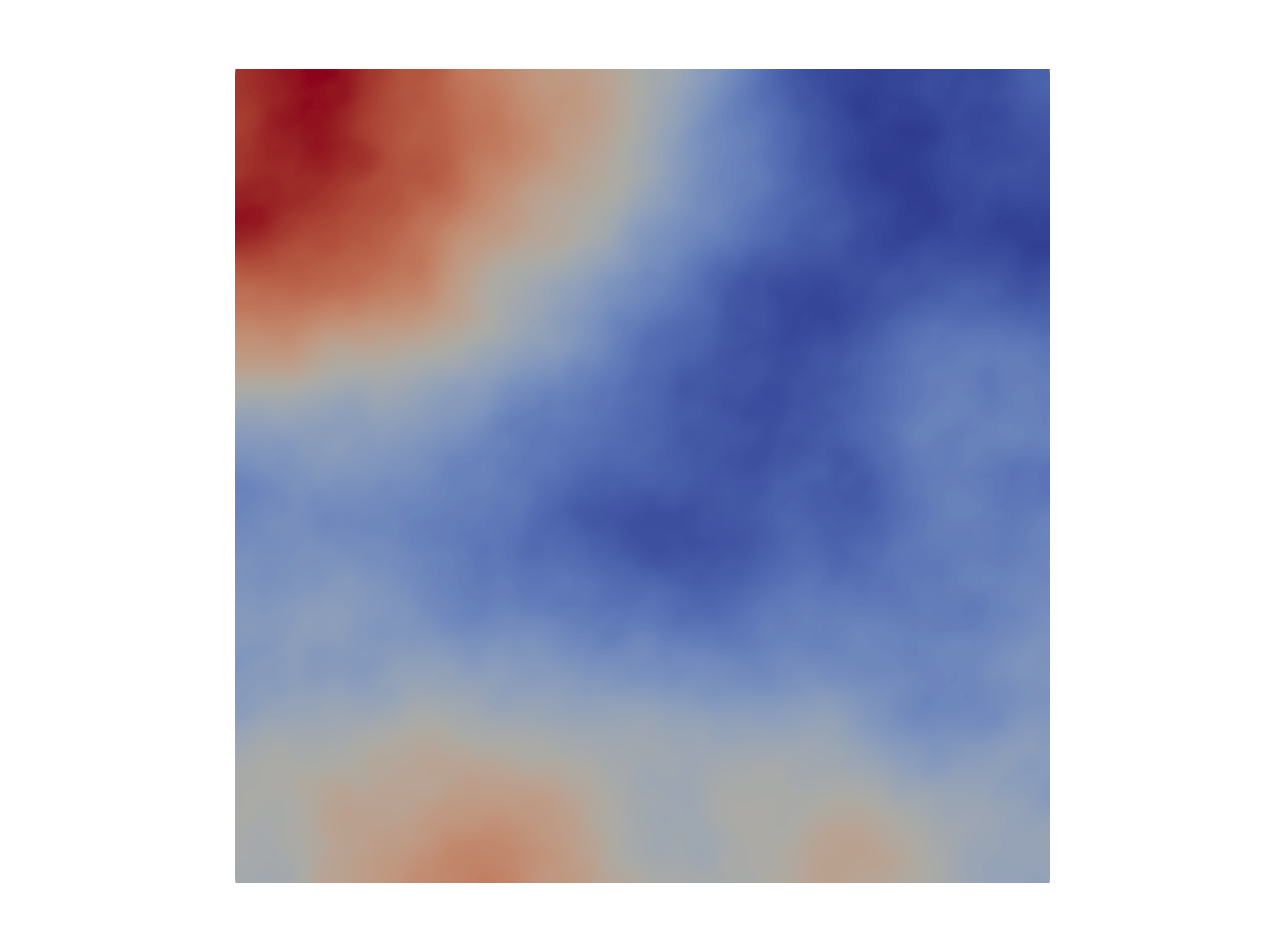
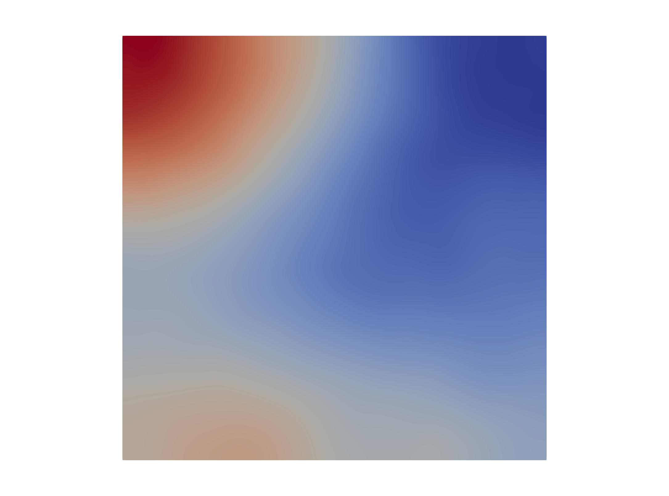
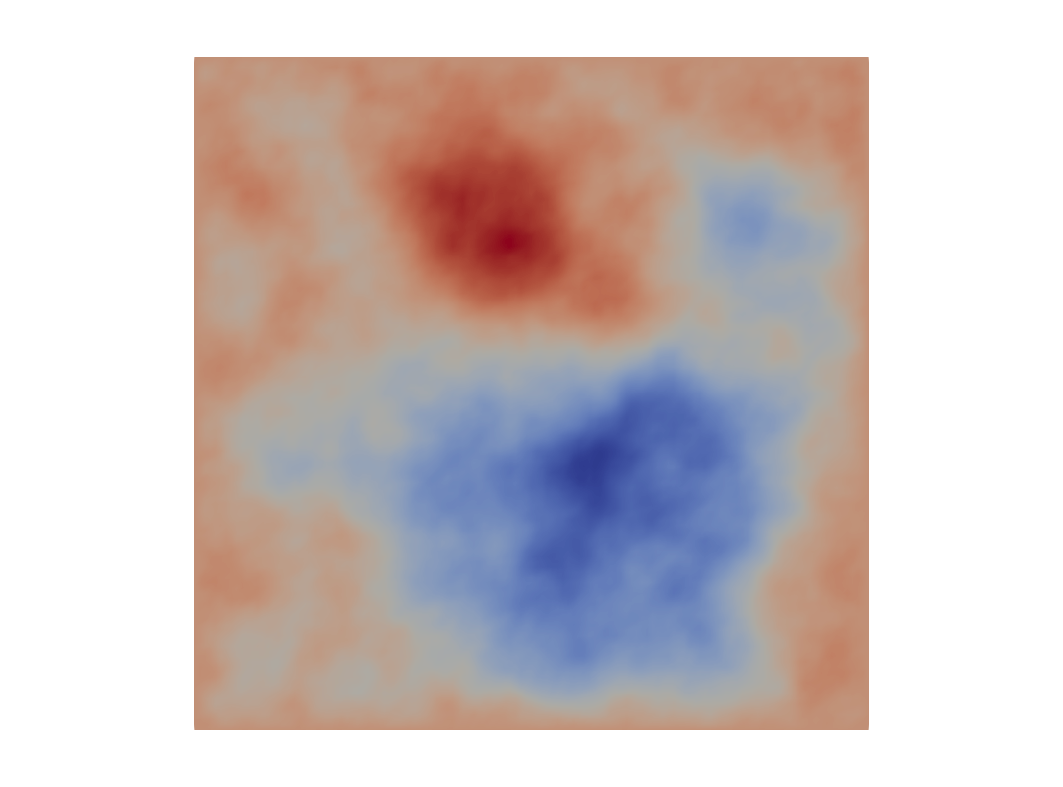
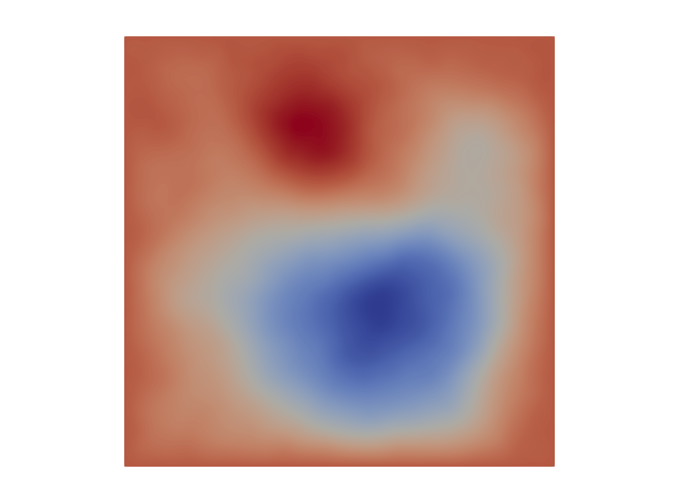
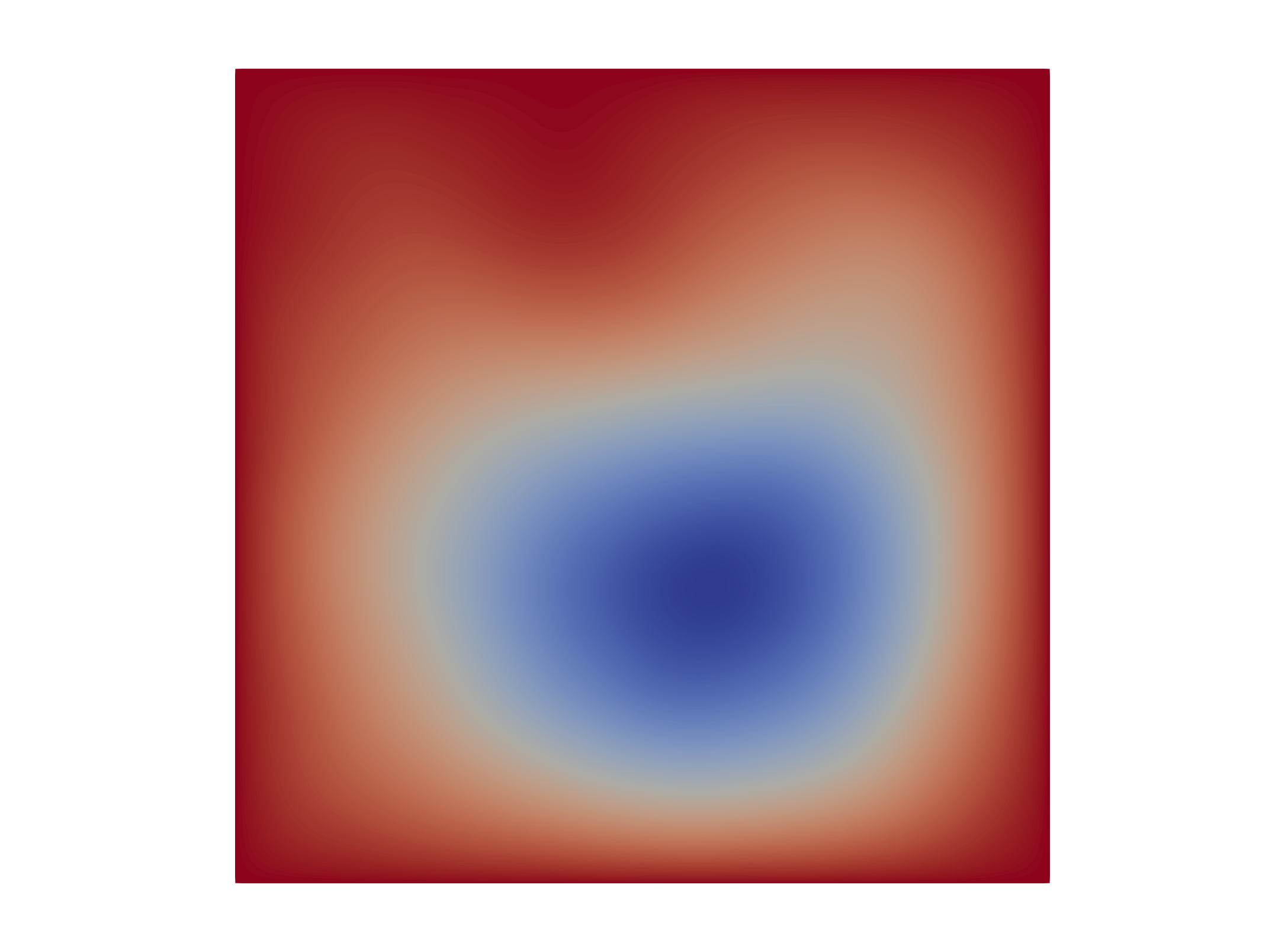
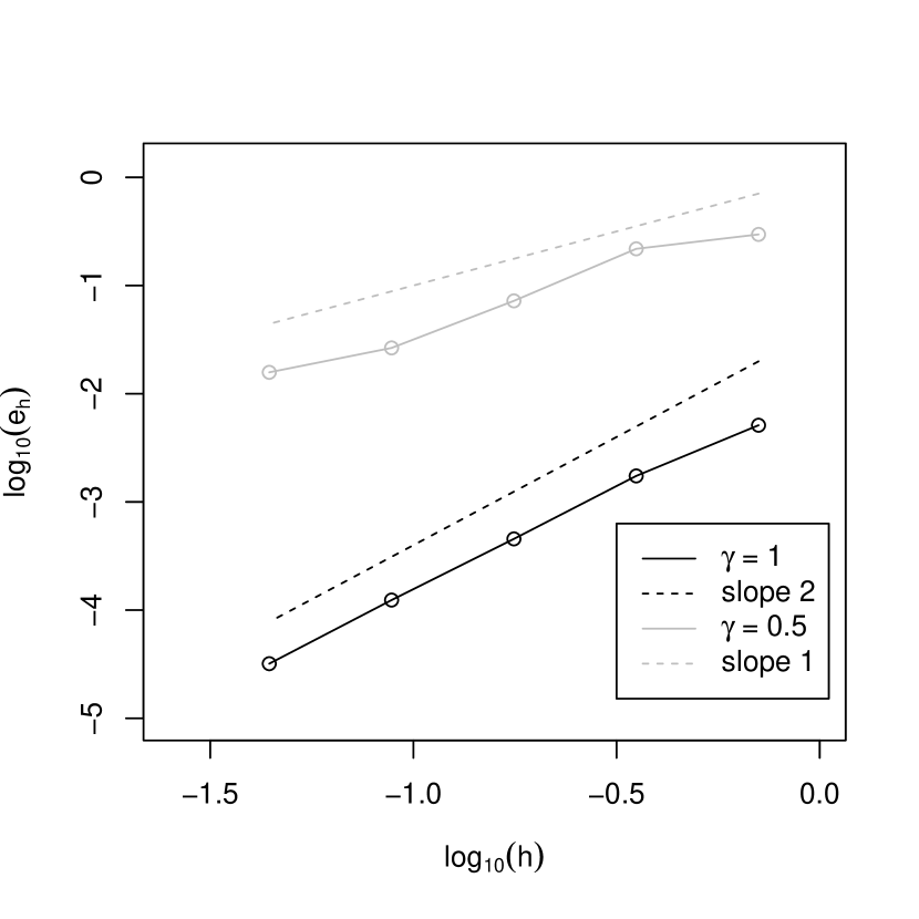
For both examples in Figure 2 we have used $T=1$ fixed $\Delta t=2^{-14}$, $k=0.1$, and a reference resolution with $h=2^{-7+1/2}$. For $\gamma=1$ the behaviour agrees with what we would expect asymptotically, while for $\gamma=0.5$ it is not as apparent. By computational restrictions, we were not able to run the $\gamma=0.5$ example with finer parameter values. The implementation is available at https://github.com/oyvinda/nested-sfem.

Appendix A Proofs of mild solution existence, and space and time regularity

Proof of Lemma 2.3.

This follows by the proof of Theorem 7.2 in [12], provided $\gamma$ is large enough for,

(28) $$E[\int_{0}^{T}\|S_{1}(T-t)A_{2}^{-\gamma}\|_{L_{2}(H)}^{2}\,dt]<\infty.$$

To show that (28) holds for any $\gamma>d/4-1/2$, we first note that owing to condition (M6): of Assumption 2.2,

$$\|(\lambda+A_{1})^{\alpha}A_{2}^{\beta}\|_{L_{2}(H)} =\|(\lambda+A_{1})^{\alpha}A_{2}^{-\alpha}A_{2}^{\alpha}A_{2}^{\beta}\|_{L_{2}(H)}$$

$$\leq\|(\lambda+A_{1})^{\alpha}A_{2}^{-\alpha}\|_{L(H)}\|A_{2}^{\alpha+\beta}\|_{L_{2}(H)}$$

$$\leq C\|A_{2}^{\alpha+\beta}\|_{L_{2}(H)}.$$

By combining Lemma 2.1 with condition (M6): and a similar computation, we also see that,

$$\|S_{1}(t)A_{2}^{\alpha}\|_{L(X)}=\|S_{1}(t)(\lambda+A_{1})^{\alpha}(\lambda+A_{1})^{-\alpha}A_{2}^{\alpha}\|_{L(X)}\leq C_{\alpha}e^{\lambda t}t^{-\alpha},\quad\alpha\geq 0.$$

This in turn gives,

$$\int_{0}^{T}\|S_{1}(t)A_{2}^{-\gamma}\|_{L_{2}(H)}^{2}\,dt =\int_{0}^{T}\|S_{1}(t)A_{2}^{1/2-\epsilon}A_{2}^{-1/2+\epsilon-\gamma}\|_{L_{2}(H)}^{2}$$

$$\leq\int_{0}^{T}\|S_{1}(t)A_{2}^{1/2-\epsilon}\|_{L(H)}^{2}\|A_{2}^{-1/2+\epsilon-\gamma}\|_{L_{2}(H)}^{2}$$

$$\leq Ce^{\lambda T}\int_{0}^{T}t^{-1+2\epsilon}\|A_{2}^{-1/2+\epsilon-\gamma}\|_{L_{2}(H)}^{2}$$

$$\leq C_{\epsilon}T^{2\epsilon}e^{\lambda T}\|A_{2}^{-1/2+\epsilon-\gamma}\|_{L_{2}(H)}^{2}<\infty,$$

since $\gamma>d/4-1/2$ and $\epsilon$ can be chosen arbitrarily small. ∎

Proof of Lemma 2.4.

The mild solution satisfies,

$$u(t)=S_{1}(t)\xi+\int_{0}^{t}S_{1}(t-s)F(u(s))\,ds+\int_{0}^{t}S_{1}(t-s)A_{2}^{-\gamma}\,dW,$$

and using that $(\lambda+A_{1})^{\alpha}$ is closed (see e.g. Theorem 6.8 in [28]), we find that,

$$(\lambda+A_{1})^{\alpha}u(t)=(\lambda+A_{1})^{\alpha}S_{1}(t)\xi+\int_{0}^{t}(\lambda+A_{1})^{\alpha}S_{1}(t-s)F(u(s))\,ds+\int_{0}^{t}(\lambda+A_{1})^{\alpha}S_{1}(t-s)A_{2}^{-\gamma}\,dW.$$

For the first term above, we have by Lemma 2.1,

$$\|(\lambda+A_{1})^{\alpha}S(t)\xi\|_{L^{p}(\Omega;H)}^{p} =E[\|(\lambda+A_{1})^{\alpha-\rho}S(t)(\lambda+A_{1})^{\rho}\xi\|_{H}^{p}]$$

$$=E[Ct^{-p\alpha+p\rho}\|(\lambda+A_{1})^{\rho}\xi\|_{H}^{p}]$$

$$=Ct^{-p\alpha+p\rho}\|(\lambda+A_{1})^{\rho}\xi\|_{L^{p}(\Omega;H)}^{p}.$$

For the next term, we have using Lemma 2.1, condition (M9): of Assumption 2.2 and finally Lemma 2.3,

$$\|\int_{0}^{t}(\lambda+A_{1})^{\alpha}S(t-s)F(u(s))\,ds\|_{L^{p}(\Omega;H)} \leq\int_{0}^{t}\|(\lambda+A_{1})^{\alpha}S_{1}(t-s)F(u(s))\|_{L^{p}(\Omega;H)}\,ds$$

$$=\int_{0}^{t}E[\|(\lambda+A_{1})^{\alpha}S_{1}(t-s)F(u(s))\|_{H}^{p}]^{1/p}\,ds$$

$$\leq\int_{0}^{t}E[\|(\lambda+A_{1})^{\alpha}S_{1}(t-s)\|_{L(H)}^{p}\|F(u(s))\|_{H}^{p}]^{1/p}\,ds]$$

$$\leq\int_{0}^{t}C(t-s)^{-\alpha}E[\|u(s)\|_{H}^{p}]^{1/p}\,ds$$

$$\leq C_{\alpha}(1+\|\xi\|_{L^{p}(\Omega;H)}^{p}),$$

provided $\alpha\in[0,1)$. For the final term, we have using Theorem 4.36 in [12],

$$\|\int_{0}^{t}(\lambda+A_{1})^{\alpha}S_{1}(t-s)A_{2}^{-\gamma}\,dW\|_{L^{p}(\Omega;H)}^{p} \leq C_{p}\bigg{(}\int_{0}^{t}\|(\lambda+A_{1})^{\alpha}S_{1}(t-s)A_{2}^{-\gamma}\|_{L_{2}(H)}^{2}\,ds\bigg{)}^{p/2}.$$

By using condition (M5): , (M6): and (M7): of Assumption 2.2, we see that for some $\epsilon\in(0,\gamma-d/4+1/2)$, the integrand satisfies,

$$\|(\lambda+A_{1})^{\alpha}S_{1}(t-s)A_{2}^{-\gamma}\|_{L_{2}(H)}^{2} =\|S_{1}(t-s)(\lambda+A_{1})^{\alpha-\gamma+d/4+\epsilon}(\lambda+A_{1})^{\gamma-d/4-\epsilon}A_{2}^{-\gamma+d/4+\epsilon}A_{2}^{-d/4-\epsilon}\|_{L_{2}(H)}^{2}$$

$$\leq Ct^{-2\alpha+2\gamma-d/2-2\epsilon}\|A_{2}^{-d/4-\epsilon}\|_{L_{2}(H)}^{2}.$$

Therefore, the integrand is integrable for any $\alpha<\gamma+1/2-d/4$ (since we can choose $\epsilon$ arbitrarily small).

Combining all of these inequalities, in addition to the fact that for $\alpha\in[0,1]$,

$$\|\xi\|_{H}\leq C\|(\lambda+A_{1})^{\alpha}\xi\|_{H},\quad\xi\in D((\lambda+A_{1})^{\alpha}),$$

(see e.g. Corollary 6.11 in [28]) finishes the proof. Note that the constant $C_{\alpha,p}$ may depend on $T$ as well, but we omit this dependence in the notation since it is not important. ∎

Proof of Lemma 2.5.

We decompose the difference as follows,

$$u(t_{2})-u(t_{1}) =(S_{1}(t_{2})-S_{1}(t_{1}))\xi+\bigg{(}\int_{0}^{t_{2}}S_{1}(t_{2}-s)F(u(s))\,ds-\int_{0}^{t_{1}}S_{1}(t_{1}-s)F(u(s))\,ds\bigg{)}$$

$$+\bigg{(}\int_{0}^{t_{2}}S_{1}(t_{2}-s)A_{2}^{-\gamma}\,dW-\int_{0}^{t_{1}}S_{1}(t_{1}-s)A_{2}^{-\gamma}\,dW\bigg{)}$$

$$=(I)+(II)+(III).$$

For $(I)$ we use Lemma 2.1 (6):

$$\|(S_{1}(t_{2})-S_{1}(t_{1}))\xi\|_{L^{p}(\Omega;H)} =E[\|(S_{1}(t_{2})-S_{1}(t_{1}))\xi\|_{H}^{p}]^{1/p}$$

$$=E[\|(S_{1}(t_{2}-t_{1})-I)(\lambda+A_{1})^{-\alpha}(\lambda+A_{1})^{\alpha-\rho}S_{1}(t_{1})(\lambda+A_{1})^{\rho}\xi\|_{H}^{p}]^{1/p}$$

$$\leq E[\|(S_{1}(t_{2}-t_{1})-I)(\lambda+A_{1})^{-\alpha}\|_{L(H)}^{p}\|(\lambda+A_{1})^{\alpha-\rho}S_{1}(t_{1})\|_{L(H)}^{p}\|(\lambda+A_{1})^{\rho}\xi\|_{H}^{p}]^{1/p}$$

$$\leq C(t_{2}-t_{1})^{\alpha}t^{-\alpha+\rho}E[\|(\lambda+A_{1})^{\rho}\xi\|_{H}^{p}]^{1/p},$$

for some $\alpha\in[0,1]$ and $\rho\in[0,\alpha]$.

For $(II)$ we have,

$$\int_{0}^{t_{2}}S_{1}(t_{2}-s)F(u(s))\,ds-\int_{0}^{t_{1}}S_{1}(t_{1}-s)F(u(s))\,ds$$

$$=\int_{0}^{t_{1}}(S_{1}(t_{2}-s)-S_{1}(t_{1}-s))F(u(s))\,ds+\int_{t_{1}}^{t_{2}}S_{1}(t_{2}-s)F(u(s))\,ds$$

$$=(i)+(ii).$$

For $(i)$ we have for some $\epsilon>0$ small, using Lemma 2.1, condition (M9): of Assumption 2.2, and finally Lemma 2.3,

$$\|\int_{0}^{t_{1}}(S_{1}(t_{2}-s)-S_{1}(t_{1}-s))F(u(s))\,ds\|_{L^{p}(\Omega;H)}$$

$$\leq\int_{0}^{t_{1}}\|(S_{1}(t_{2}-s)-S_{1}(t_{1}-s))F(u(s))\|_{L^{p}(\Omega;H)}\,ds$$

$$=\int_{0}^{t_{1}}E[\|(S_{1}(t_{2}-s)-S_{1}(t_{1}-s))F(u(s))\|_{H}^{p}]^{1/p}\,ds$$

$$=\int_{0}^{t_{1}}E[\|(S_{1}(t_{2}-t_{1})-I)S_{1}(t_{1}-s)F(u(s))\|_{H}^{p}]^{1/p}\,ds$$

$$=\int_{0}^{t_{1}}E[\|(S_{1}(t_{2}-t_{1})-I)(\lambda+A_{1})^{-1+\epsilon}(\lambda+A_{1})^{1-\epsilon}S_{1}(t_{1}-s)F(u(s))\|_{H}^{p}]^{1/p}\,ds$$

$$\leq\int_{0}^{t_{1}}E[\|(S_{1}(t_{2}-t_{1})-I)(\lambda+A_{1})^{-1+\epsilon}\|_{L(H)}^{p}\|(\lambda+A_{1})^{1-\epsilon}S_{1}(t_{1}-s)\|_{L(H)}^{p}\|F(u(s))\|_{H}^{p}]^{1/p}\,ds$$

$$\leq\int_{0}^{t_{1}}C(t_{2}-t_{1})^{1-\epsilon}(t_{1}-s)^{-1+\epsilon}E[\|F(u(s))\|_{H}^{p}]^{1/p}\,ds$$

$$\leq\int_{0}^{t_{1}}C(t_{2}-t_{1})^{1-\epsilon}(t_{1}-s)^{-1+\epsilon}E[\|u(s)\|_{H}^{p}]^{1/p}\,ds$$

$$\leq C_{\epsilon}(t_{2}-t_{1})^{1-\epsilon}(1+\|\xi\|_{L^{p}(\Omega;H)}).$$

For $(ii)$, we have by the boundedness of $S_{1}(t)$, condition (M9): of Assumption 2.2 and finally Lemma 2.3,

$$\|\int_{t_{1}}^{t_{2}}S_{1}(t_{2}-s)F(u(s))\,ds\|_{L^{p}(\Omega;H)} \leq\int_{t_{1}}^{t_{2}}\|S_{1}(t_{2}-s)F(u(s))\|_{L^{p}(\Omega;H)}\,ds$$

$$=\int_{t_{1}}^{t_{2}}E[\|S_{1}(t_{2}-s)F(u(s))\|_{H}^{p}]^{1/p}$$

$$\leq\int_{t_{1}}^{t_{2}}E[\|S_{1}(t_{2}-s)\|_{L(H)}^{p}\|F(u(s))\|_{H}^{p}]^{1/p}$$

$$\leq C\int_{t_{1}}^{t_{2}}E[\|F(u(s))\|_{H}^{p}]^{1/p}\,ds$$

$$\leq C(t_{2}-t_{1})(1+\|\xi\|_{L^{p}(\Omega;H)}).$$

For $(III)$, we have,

$$\int_{0}^{t_{2}}S_{1}(t_{2}-s)A_{2}^{-\gamma}\,dW-\int_{0}^{t_{1}}S_{1}(t_{1}-s)A_{2}^{-\gamma}\,dW =\int_{0}^{t_{1}}(S_{1}(t_{2}-s)-S_{1}(t_{1}-s))A_{2}^{-\gamma}\,dW$$

$$+\int_{t_{1}}^{t_{2}}S_{1}(t_{2}-s)A_{2}^{-\gamma}\,dW$$

$$=(i)+(ii).$$

For $(i)$ we have using Theorem 4.36 in [12],

$$\|\int_{0}^{t_{1}}(S_{1}(t_{2}-s)-S_{1}(t_{1}-s))A_{2}^{-\gamma}\,dW\|_{L^{p}(\Omega;H)}^{p}\leq C_{p}\bigg{(}\int_{0}^{t_{1}}\|(S_{1}(t_{2}-s)-S_{1}(t_{1}-s))A_{2}^{-\gamma}\|_{L_{2}(H)}^{2}\,ds\bigg{)}^{p/2}.$$

For the integrand, we have by condition (M5): and (M6): of Assumption 2.2 and some $\epsilon>0$ small,

$$\|(S_{1}(t_{2}-s)-S_{1}(t_{1}-s))A_{2}^{-\gamma}\|_{L_{2}(H)}^{2} =\|(S_{1}(t_{2}-t_{1})-I)S(t_{1}-s)A_{2}^{-\gamma+d/4+\epsilon}A_{2}^{-d/4-\epsilon}\|_{L_{2}(H)}^{2}$$

$$\leq\|(S_{1}(t_{2}-t_{1})-I)S_{1}(t_{1}-s)(\lambda+A_{1})^{-\gamma+d/4+\epsilon}\|_{L(H)}^{2}$$

$$\times\|(\lambda+A_{1})^{\gamma-d/4-\epsilon}A_{2}^{-\gamma+d/4+\epsilon}\|_{L(H)}^{2}$$

$$\times\|A_{2}^{-d/4-\epsilon}\|_{L_{2}(H)}^{2}$$

$$\leq C_{\epsilon}\|(S_{1}(t_{2}-t_{1})-I)S_{1}(t_{1}-s)(\lambda+A_{1})^{-\gamma+d/4+\epsilon}\|_{L(H)}^{2}.$$

By using Lemma 2.1, (6), we get,

$$\|(S_{1}(t_{2}-t_{1})-I)S_{1}(t_{1}-s)(\lambda+A_{1})^{-\gamma+d/4+\epsilon}\|_{L(H)}^{2}$$

$$=\|(S_{1}(t_{2}-t_{1})-I)(\lambda+A_{1})^{-\gamma+d/4+2\epsilon-1/2}A^{1/2-\epsilon}S_{1}(t_{1}-s)\|_{L(H)}^{2}$$

$$\leq(t_{2}-t_{1})^{2\gamma+1-d/2-4\epsilon}(t_{1}-s)^{-1+2\epsilon},$$

and we must therefore have,

$$\|(i)\|_{L^{p}(\Omega;H)}\leq C_{\epsilon}(t_{2}-t_{1})^{\gamma+1/2-d/4-\epsilon}.$$

For $(ii)$ we have by Theorem 4.36 in [12],

$$\|\int_{t_{1}}^{t_{2}}S_{1}(t_{2}-s)A_{2}^{-\gamma}\,dW\|_{L^{p}(\Omega;H)}^{p}\leq C_{p}\bigg{(}\int_{t_{1}}^{t_{2}}\|S_{1}(t_{2}-s)A_{2}^{-\gamma}\|_{L_{2}(H)}^{2}\,ds\bigg{)}^{p/2}.$$

For the integrand, we have by condition (M5): of Assumption 2.2, and for some $\epsilon>0$ small,

$$\|S_{1}(t_{2}-s)A_{2}^{-\gamma+d/4+\epsilon}A_{2}^{-d/4-\epsilon}\|_{L_{2}(H)}^{2} \leq\|S_{1}(t_{2}-s)A_{2}^{-\gamma+d/4+\epsilon}\|_{L(H)}^{2}\|A_{2}^{-d/4-\epsilon}\|_{L_{2}(H)}^{2}$$

$$\leq C_{\epsilon}\begin{cases}(t_{2}-s)^{2\gamma-d/2-2\epsilon},\quad&\gamma-d/4-\epsilon<0,\\ 1,\quad&\text{otherwise}.\end{cases}$$

By evaluating the integral, we therefore, have,

$$\|(ii)\|_{L^{p}(\Omega;H)}\leq C_{\epsilon}\begin{cases}(t_{2}-t_{1})^{\gamma+1/2-d/4-\epsilon},\quad&\gamma-d/4-\epsilon<0,\\ (t_{2}-t_{1})^{1/2},\quad&\text{otherwise}.\end{cases}$$

Combining all of these inequalities, in addition to the fact that for $\alpha\in[0,1]$,

$$\|\xi\|_{H}\leq C\|(\lambda+A_{1})^{\alpha}\xi\|_{H},\quad\xi\in D((\lambda+A_{1})^{\alpha}),$$

(see e.g. Corollary 6.11 in [28]) finishes the proof (also here the constant may depend on $T$). ∎

Appendix B Derivation of (21) and (22)

Before we move on to the derivation of (21), (22) we state the proof of Lemma 3.4.

Proof of Lemma 3.4.

First we assert that $\pi_{h}\in L_{2}(H)$. Let $\{e_{j}\}_{j=1}^{\infty}$ be an $H$-orthonormal basis of $H$, $\{e_{h,j}\}_{j=1}^{\infty}$ the $H$-orthonormal basis of $V_{h}$, and note that,

$$\|\pi_{h}\|_{L_{2}(H)}^{2} =\sum_{j=1}^{\infty}\|\pi_{h}e_{j}\|_{H}^{2}=\sum_{j=1}^{\infty}(\pi_{h}e_{j},\pi_{h}e_{j})_{H}=\sum_{j=1}^{\infty}(\sum_{k=1}^{N_{h}}(e_{j},e_{h,k})_{H}e_{k,h},\sum_{l=1}^{N_{h}}(e_{j},e_{h,l})_{H}e_{l,h})_{H}$$

$$=\sum_{k=1}^{N_{h}}\sum_{l=1}^{N_{h}}\sum_{j=1}^{\infty}(e_{j},e_{h,k})_{H}(e_{j},e_{h,l})_{H}(e_{h,l},e_{h,k})_{H},$$

and using the orthonormality of $\{e_{h,j}\}$, we get that the expansion above reduces to,

$$\sum_{k=1}^{N_{h}}\sum_{j=1}^{\infty}(e_{j},e_{h,k})_{H}(e_{j},e_{h,k})_{H}=\sum_{k=1}^{N_{h}}(e_{h,k},e_{h,k})_{H}=N_{h}.$$

It follows that $\|\pi_{h}\|_{L_{2}(H)}=N_{h}^{1/2}$. By definition of $W$, we have,

$$W(t):=\sum_{j=1}^{\infty}\beta_{j}^{\prime}(t)e_{j},\quad P\text{-a.s.}$$

for some independent Brownian motions $\{\beta_{j}^{\prime}\}_{j}$, where the equality holds $P$-a.s., with equality in any larger Hilbert space where the inclusion is Hilbert-Schmidt (see e.g. Proposition 4.7 in [12]). Defining,

$$\pi_{h}W(t):=\sum_{j=1}^{\infty}\beta_{j}^{\prime}(t)\pi_{h}e_{j},$$

we have that $\pi_{h}W$ is a Wiener process with covariance operator $\pi_{h}(\pi_{h})^{*}=\pi_{h}$. Since $\pi_{h}$ is compact and selfadjoint, it admits an $H$-orthonormal basis of $H$ of eigenvectors. Since $\pi_{h}^{2}=\pi_{h}$ and $\pi_{h}$ has rank $N_{h}$, we must have that the eigenvalues $\lambda_{j}$ (after reordering) are $1$ for $j=1,\dots,N_{h}$, while $\lambda_{j}=0$ for $j>N_{h}$. We may take the corresponding eigenvectors to by $e_{h,j}$ above, and by expressing this $\pi_{h}$-Wiener process as an expansion in terms of the eigenvectors $\{e_{h,j}\}_{j}$ of $\pi_{h}$ (see e.g. Proposition 4.3 in [12]), we have that,

$$\pi_{h}W(t)=\sum_{j=1}^{\infty}\sqrt{\lambda_{j}}\beta_{j}(t)e_{h,j}=\sum_{j=1}^{N_{h}}\beta_{j}(t)e_{h,j},$$

$P$-a.s. for some independent scalar Brownian motions $\{\beta_{j}\}_{j=1}^{N_{h}}$. ∎

In order to derive (21), (22) we first note that solving (19) (with $F=0$) is the same as solving the system on equations,

(29) $$((I+\Delta tA_{1,h})u_{h,\Delta t}(t_{n+1}),\varphi_{j})_{H}=(u_{h,\Delta t}(t_{n})+Q_{k}^{-\gamma}(A_{2,h})\pi_{h}(W(t_{n+1})-W(t_{n})),\varphi_{j})_{H},\quad j=1,\dots,N_{h},$$

where $\{\varphi_{j}\}_{j=1}^{N_{h}}$ is the nodal basis of $V_{h}$. To set up this system, the following lemma will be useful.

Lemma B.1.

For $\gamma=1$, we have,

$$A_{2,h}^{-1}\pi_{h}(W(t_{n+1})-W(t_{n}))=\sum_{j=1}^{N_{h}}\theta_{j}\varphi_{j},$$

$P$-a.s, where,

$$\theta=\sqrt{\Delta t}K_{h}^{-1}\sqrt{M_{h}}\varrho^{n}.$$

Here $(\cdot)_{j}$ denotes the $j$’th entry of a vector, $\varrho^{n}\sim\mathcal{N}(0,I)$ are $N_{h}$-dimensional multivariate Gaussian, and $\sqrt{M_{h}}$ is some square root of $M_{h}$. If $\gamma\in(0,1)$, we have,

$$Q_{k}^{-\gamma}(A_{2,h})\pi_{h}(W(t_{n+1})-W(t_{n}))=\sum_{j=1}^{N_{h}}\theta_{j}^{\prime}\varphi_{j},$$

$P$-a.s., where,

$$\theta^{\prime}=\sqrt{\Delta t}\frac{k\sin(\pi\gamma)}{\pi}\sum_{l=-M}^{N}e^{(1-\gamma)y_{l}}(e^{y_{l}}M_{h}+K_{h})^{-1}\sqrt{M_{h}}\varrho^{n}.$$

Proof.

Set for ease of notation,

$$f:=\pi_{h}(W(t_{n+1})-W(t_{n})).$$

By lemma 3.4, one has that $f$ is an $H$-valued Gaussian random variable, with covariance operator $\Delta t\pi_{h}$.

For the first idenity of the lemma, note that $A_{2,h}^{-1}f$ is the solution $g\in V_{h}$ of

$$A_{2,h}g=f.$$

Since $f\in V_{h}$ $P$-a.s. by Lemma 3.4, solving the equation above is the same as solving the system of equations,

(30) $$\begin{pmatrix}(A_{2,h}g,\varphi_{1})_{H}\\ \vdots\\ (A_{2,h}g,\varphi_{N_{h}})_{H}\end{pmatrix}=\begin{pmatrix}(f,\varphi_{1})_{H}\\ \vdots\\ (f,\varphi_{N_{h}})_{H}\end{pmatrix}.$$

By Lemma 3.4 we have,

$$E[(f,\varphi_{i})_{H}(f,\varphi_{j})_{H}]=\Delta t(\varphi_{i},\varphi_{j})_{H},$$

and so the covariance matrix of $((f,\varphi_{1})_{H},\dots,(f,\varphi_{N_{h}}))^{T}$ is the (scaled) mass matrix, $\Delta tM_{h}$ (as defined in (20)). It follows that we can construct some multivariate Gaussian $\varrho^{n}\sim\mathcal{N}(0,I)$ such that,

$$((f,\varphi_{1})_{H},\dots,(f,\varphi_{N_{h}}))^{T}=\sqrt{\Delta t}\sqrt{M_{h}}\varrho^{n},$$

$P$-a.s. For the left hand side of (30) we insert $g=\sum_{j=1}^{N_{h}}\theta_{j}\varphi_{j}$, and find, using that $(A_{2,h}\varphi_{j},\varphi_{i})_{H}=a_{2}(\varphi_{j},\varphi_{i})$,

$$\begin{pmatrix}(A_{2,h}g,\varphi_{1})_{H}\\ \vdots\\ (A_{2,h}g,\varphi_{N_{h}})_{H}\end{pmatrix}=K_{h}\begin{pmatrix}\theta_{1}\\ \vdots\\ \theta_{N_{h}}\end{pmatrix},$$

where $K_{h}$ is as in (20). Combining these observations, we see that (30) has solution $(g_{1},\dots,g_{N_{h}})$ given by,

$$(g_{1},\dots,g_{N_{h}})^{T}=\sqrt{\Delta t}K_{h}^{-1}\sqrt{M_{h}}\varrho^{n}.$$

For the second identity of the lemma we argue similarly: note that,

$$Q_{k}^{-\gamma}(A_{2,h})f=\frac{k\sin(\pi\gamma)}{\pi}\sum_{j=-M}^{N}e^{(1-\gamma)y_{j}}g^{(j)},$$

where $g^{(j)}\in V_{h}$, is the solution of the equation,

$$(e^{y_{j}}I+A_{2,h})g^{(j)}=f,\quad j=-M,\dots,N.$$

As for the previous term, to solve this equation we insert $g^{(j)}=\sum_{l=1}^{N_{h}}\theta^{(j)}_{l}\varphi_{l}$ into the equation and integrate against the nodal basis, to find,

$$(e^{y_{j}}M_{h}+K_{h})\begin{pmatrix}\theta_{1}^{(j)}\\ \vdots\\ \theta_{N_{h}}^{(j)}\end{pmatrix}=\sqrt{\Delta t}\sqrt{M_{h}}\varrho^{n}.$$

Summing up the vectors $(\theta^{(j)}_{1},\dots,\theta^{(j)}_{N_{h}}),\ j=-M,\dots,N$ we find the coeffcients of $Q_{k}^{-\gamma}f$ in the nodal basis, $\theta^{\prime}$. This gives the second identity of the lemma. ∎

Now we can insert the identities of Lemma B.1 into the system of equations (29) to arrive at (21) and (22): note that for any $g=\sum_{j=1}^{N_{h}}\theta_{j}\varphi_{j}$, we have,

$$\begin{pmatrix}(g,\varphi_{1})_{H}\\ \vdots\\ (g,\varphi_{N_{h}})_{H}\end{pmatrix}=M_{h}\theta,$$

and so,

$$\begin{pmatrix}((I+\Delta tA_{1,h})u_{h,\Delta t}(t_{n+1}),\varphi_{1})_{H}\\ \vdots\\ ((I+\Delta tA_{1,h})u_{h,\Delta t}(t_{n+1}),\varphi_{N_{h}})_{H}\end{pmatrix}=(M_{h}+\Delta tT_{h})\alpha^{n+1},$$

while,

$$\begin{pmatrix}(Q_{k}^{-\gamma}(A_{2,h})\pi_{h}(W(t_{n+1})-W(t_{n})),\varphi_{1})_{H}\\ \vdots\\ (Q_{k}^{-\gamma}(A_{2,h})\pi_{h}(W(t_{n+1})-W(t_{n})),\varphi_{N_{h}})_{H}\end{pmatrix}$$

$$=\begin{cases}M_{h}\sqrt{\Delta t}\frac{k\sin(\pi\gamma)}{\pi}\sum_{j=-M}^{N}e^{(1-\gamma)y_{j}}(e^{y_{j}}M_{h}+K_{h})^{-1}\sqrt{M_{h}}\varrho^{n},\quad&\gamma\in(0,1),\\ M_{h}\sqrt{\Delta t}K_{h}^{-1}\sqrt{M_{h}}\varrho^{n},\quad&\gamma=1.\end{cases}$$

References

- [1] Rikard Anton, David Cohen and Lluis Quer-Sardanyons “A fully discrete approximation of the one-dimensional stochastic heat equation” In IMA J. Numer. Anal. 40.1, 2020, pp. 247–284
- [2] Yagi Atsushi “Abstract Parabolic Evolution Equations and their Applications” Springer, 2010
- [3] Øyvind Stormark Auestad “Numerical Approximation of Linear Evolution Equations Revisited” In arXiv, 2024
- [4] Andrea Barth and Annika Lang “ and almost sure convergence of a Milstein scheme for stochastic partial differential equations” In Stochastic Process. Appl. 123.5, 2013, pp. 1563–1587
- [5] Sebastian Becker and Arnulf Jentzen “Strong convergence rates for nonlinearity-truncated Euler-type approximations of stochastic Ginzburg-Landau equations” In Stochastic Process. Appl. 129.1, 2019, pp. 28–69
- [6] David Bolin, Kristin Kirchner and Mihály Kovács “Numerical solution of fractional elliptic stochastic PDEs with spatial white noise” In IMA J. Numer. Anal. 40.2, 2018, pp. 1051–1073
- [7] David Bolin, Kristin Kirchner and Mihály Kovács “Weak convergence of Galerkin approximations for fractional elliptic stochastic PDEs with spatial white noise” In BIT 58.4, 2018, pp. 881–906
- [8] Andrea Bonito, Diane Guignard and Wenyu Lei “Numerical approximation of gaussian random fields on closed surfaces” In Comput. Methods Appl. Math., 2022
- [9] Andrea Bonito, Wenyu Lei and Joseph E. Pasciak “On sinc quadrature approximations of fractional powers of regularly accretive operators” In Numer. Math. 27.2, 2019, pp. 57–68
- [10] Sonja Cox and Jan Neerven “Pathwise Hölder convergence of the implicit-linear Euler scheme for semi-linear SPDEs with multiplicative noise” In Numer. Math. 125.2, 2013, pp. 259–345
- [11] Sonja G. Cox and Kristin Kirchner “Regularity and convergence analysis in Sobolev and Hölder spaces for generalized Whittle–Matérn fields” In Numer. Math. 146.4 Springer ScienceBusiness Media LLC, 2020, pp. 819–873
- [12] Giuseppe Da Prato and Jerzy Zabczyk “Stochastic Equations in Infinite Dimensions” Cambridge university texts, 2014
- [13] Istvan Gyöngy and Annie Millet “Rate of convergence of space time approximations for stochastic evolution equations” In Potential Anal. 30.1, 2009, pp. 29–64
- [14] Claudine Hallern and Andreas Rössler “An Analysis of the Milstein Scheme for SPDEs Without a Commutative Noise Condition” In Monte Carlo and Quasi-Monte Carlo Methods 324 Cham: Springer International Publishing, 2020, pp. 503–521
- [15] Lukas Herrmann, Kristin Kirchner and Christoph Schwab “Multilevel approximation of Gaussian random fields: fast simulation” In Math. Models Methods Appl. Sci. 30.01, 2020, pp. 181–223
- [16] Erik Jansson, Mihály Kovács and Annika Lang “Surface finite element approximation of spherical Whittle-Matérn Gaussian random fields” In SIAM J. Sci. Comput. 44.2, 2021, pp. A825–A842
- [17] Arnulf Jentzen and Peter Kloeden “The Numerical Approximation of Stochastic Partial Differential Equations” In Milan J. Math. 77 Springer, 2009, pp. 205–244
- [18] Arnulf Jentzen, Peter Kloeden and Georg Winkel “Efficient simulation of nonlinear parabolic SPDEs with additive noise” In Ann. Appl. Probab. 21.3, 2011, pp. 908–950
- [19] Minoo Kamrani and Dirk Blömker “Pathwise convergence of a numerical method for stochastic partial differential equations with correlated noise and local Lipschitz condition” In J. Comput. Appl. Math. 323, 2017, pp. 123–135
- [20] Mihály Kovács, Stig Larsson and Fredrik Lindgren “On the backward Euler approximation of the stochastic Allen Cahn equation” In J. Appl. Probab. 52.2, 2015, pp. 323–338
- [21] Mihály Kovács, Stig Larsson and Fredrik Lindgren “On the discretisation in time of the stochastic Allen-Cahn equation” In Math. Nachr. 291.5-6, 2015, pp. 966–995
- [22] Raphael Kruse “Optimal error estimates of Galerkin finite element methods for stochastic partial differential equations with multiplicative noise” In IMA J. Numer. Anal. 34.1, 2014, pp. 217–251
- [23] Raphael Kruse “Strong and weak approximations of semilinear stochastic evolution equations”, Springer lecture notes in mathematics Springer, 2014
- [24] Finn Lindgren, David Bolin and Håvard Rue “The SPDE approach for Gaussian and non-Gaussian fields: 10 years and still running” In Spat. Stat. 50, 2022, pp. 100599
- [25] Finn Lindgren, Håvard Rue and Johan Lindstrøm “An explicit link between Gaussian fields and Gaussian Markov random fields: the stochastic partial differential equation approach” In J. R. Stat. Soc. Ser. B. Stat. Methodol. 73.4 Oxford University Press, 2011, pp. 423–498
- [26] Gabriel J Lord and Antoine Tambue “Stochastic exponential integrators for the finite element discretization of SPDEs for multiplicative and additive noise” In IMA J. Numer. Anal. 33.2, 2013, pp. 515–543
- [27] Gabriel J. Lord, Catherine E. Powell and Tony Shardlow “An introduction to computational stochastic PDEs”, Cambridge Texts in Applied Mathematics Cambridge University Press, New York, 2014
- [28] Amnon Pazy “Semigroups of Linear Operators and Applications to Partial Differential Equations” Applied mathematical sciences, 1983
- [29] Alfio Quarteroni and Alberto Valli “Numerical Approximation of Partial Differential Equations”, Springer Series in Computational Mathematics Springer, 1994
- [30] Xiaojie Wang “Strong convergence rates of the linear implicit Euler method for the finite element discretization of SPDEs with additive noise” In IMA J. Numer. Anal. 37.2, 2016, pp. 965–984
- [31] Peter Whittle “On stationary processes in the plane” In Biometrika 41.3/4 Oxford University Press, 1954, pp. 434–449