a𝑎a-potent Schwarz matrices and Bessel-like Jacobi polynomials

Alexander Dyachenko Keldysh Institute of Applied Mathematics, Russian Academy of Sciences, 125047, Moscow, Russia diachenko@sfedu.ru Carlos M. da Fonseca Kuwait College of Science and Technology, Doha District, Safat 13133, Kuwait Chair of Computational Mathematics, University of Deusto, 48007 Bilbao, Spain c.dafonseca@kcst.edu.kw  and  Mikhail Tyaglov Department of Mathematics and Computer Sciences, St.Petersburg State University, St.Petersburg, 199178, Russia tyaglov@mail.ru
Abstract.

We consider the problem of the reconstruction of a Schwarz matrix from exactly one given eigenvalue. This inverse eigenvalue problem leads to the Jacobi orthogonal polynomials {Pk(n,n)}k=0n1superscriptsubscriptsuperscriptsubscript𝑃𝑘𝑛𝑛𝑘0𝑛1\{P_{k}^{(-n,n)}\}_{k=0}^{n-1} that can be treated as a discrete finite analogue of Bessel polynomials.

Key words and phrases:
Inverse eigenvalue problem, Schwarz matrices, unipotent matrices, orthogonal polynomials
1991 Mathematics Subject Classification:
15B05, 33C45, 15A18, 15A29, 15A15

1. Introduction

The matrix inverse eigenvalue problem consists in reconstructing a specific structured matrix from a prescribed spectral data. This topic is of great interest in different branches of mathematics, continually providing new and surprising results (see for example [10, 22, 33, 34] and the references there).

From the celebrated work [36] by Hubert S. Wall, it follows that there exists a unique matrix

(1.1) Jn=[b01b101b21bn10]subscript𝐽𝑛matrixsubscript𝑏01missing-subexpressionmissing-subexpressionmissing-subexpressionsubscript𝑏101missing-subexpressionmissing-subexpressionmissing-subexpressionsubscript𝑏2missing-subexpressionmissing-subexpressionmissing-subexpression1missing-subexpressionmissing-subexpressionmissing-subexpressionsubscript𝑏𝑛10J_{n}=\begin{bmatrix}-b_{0}&1&&&\\ -b_{1}&0&1&&\\ &-b_{2}&\ddots&\ddots&\\ &&\ddots&\ddots&1\\ &&&-b_{n-1}&0\\ \end{bmatrix}

with bk>0subscript𝑏𝑘0b_{k}>0, for k=0,1,,n1𝑘01𝑛1k=0,1,\ldots,n-1, whose characteristic polynomial is (x+1)nsuperscript𝑥1𝑛(x+1)^{n} (see also [32, 35, 37] for more details). Wall’s argumentation is based on the stability of the characteristic polynomial, i.e. on that all its zeros have negative real parts — which is of course true for (x+1)nsuperscript𝑥1𝑛(x+1)^{n}.

By analogy with nilpotent matrices, one introduces unipotent matrices: an n×n𝑛𝑛n\times n matrix is called unipotent if its characteristic polynomial is (x1)nsuperscript𝑥1𝑛(x-1)^{n}, or, equivalently, if all its eigenvalues are equal to 111. Various disciplines deal with unipotent matrices, cf. e.g. [6, 21, 28, 38]. We consider an extension of this definition, namely matrices with only a single eigenvalue labelled by a𝑎a. In brief, we are looking for an “a𝑎a-potent” matrix of the form (1.1) where a{0}𝑎0a\in\mathbb{C}\setminus\{0\}.

Matrices of the form (1.1) are called Schwarz matrices. Such matrices are very important in automatic control theory and signal processing (see, for example, [8]), and several general inverse problems have been previously considered in [3, 7, 11, 13, 16]. So, here we consider the inverse eigenvalue problem for a Schwarz matrix whose characteristic polynomial is

(1.2) p(z)=(za)n=i=0n(1)ni(ni)anizi,𝑝𝑧superscript𝑧𝑎𝑛superscriptsubscript𝑖0𝑛superscript1𝑛𝑖binomial𝑛𝑖superscript𝑎𝑛𝑖superscript𝑧𝑖p(z)=(z-a)^{n}=\sum_{i=0}^{n}(-1)^{n-i}\binom{n}{i}a^{n-i}z^{i},

where a𝑎a is a given nonzero complex number. That is, we want to construct a Schwarz matrix (1.1) with only one eigenvalue a𝑎a.

Since Jksubscript𝐽𝑘J_{k} is the leading principal k×k𝑘𝑘k\times k submatrix of Jnsubscript𝐽𝑛J_{n}, with k{1,,n}𝑘1𝑛k\in\{1,\ldots,n\}, the polynomials

Pk(z)=det(zIkJk),fork=1,,n,formulae-sequencesubscript𝑃𝑘𝑧𝑧subscript𝐼𝑘subscript𝐽𝑘for𝑘1𝑛P_{k}(z)=\det(zI_{k}-J_{k})\,,\quad\mbox{for}\;k=1,\ldots,n\,,

where Iksubscript𝐼𝑘I_{k} is the identity matrix of order k𝑘k and Pn(z)=p(z)subscript𝑃𝑛𝑧𝑝𝑧P_{n}(z)=p(z), satisfy the following three-term recurrence relation:

P0(z)subscript𝑃0𝑧\displaystyle P_{0}(z) =\displaystyle= 1,1\displaystyle 1\,,
(1.3) P1(z)subscript𝑃1𝑧\displaystyle P_{1}(z) =\displaystyle= z+b0,𝑧subscript𝑏0\displaystyle z+b_{0}\,,
Pk+1(z)subscript𝑃𝑘1𝑧\displaystyle P_{k+1}(z) =\displaystyle= zPk(z)+bkPk1(z),fork=1,,n1.formulae-sequence𝑧subscript𝑃𝑘𝑧subscript𝑏𝑘subscript𝑃𝑘1𝑧for𝑘1𝑛1\displaystyle zP_{k}(z)+b_{k}P_{k-1}(z)\,,\quad\mbox{for}\;k=1,\ldots,n-1\,.

By the Favard theorem, see111In [27], this extended version is attributed to Chihara, although in essence it already existed in [17].  [9, pp. 21–22], the sequence {Pk(z)}k=0n1superscriptsubscriptsubscript𝑃𝑘𝑧𝑘0𝑛1\{P_{k}(z)\}_{k=0}^{n-1} is orthogonal w.r.t. a linear functional. Observe that, given arbitrary n>1𝑛1n>1 and a{0}𝑎0a\in\mathbb{C}\setminus\{0\}, this functional is not positive and cannot be written as an integral w.r.t. a measure on the real line (otherwise Jnsubscript𝐽𝑛J_{n} would have n𝑛n distinct real eigenvalues). Accordingly, for n>1𝑛1n>1 the numbers b1,,bn1subscript𝑏1subscript𝑏𝑛1b_{1},\dots,b_{n-1} in (1.3) cannot be chosen negative while b0subscript𝑏0b_{0} remains real. As is seen from Section 3.2, the support of the orthogonality functional is natural to take consisting of a unique point a𝑎a.

We find the aforementioned matrix Jnsubscript𝐽𝑛J_{n}, see the values of b0subscript𝑏0b_{0} and b1,,bn1subscript𝑏1subscript𝑏𝑛1b_{1},\dots,b_{n-1} in, resp., (2.9) and (2.23). The sequence {Pk(z)}k=0n1superscriptsubscriptsubscript𝑃𝑘𝑧𝑘0𝑛1\{P_{k}(z)\}_{k=0}^{n-1} satisfying (1.3) reduces to a finite chunk of the Jacobi polynomials with non-standard parameters. The explicit expression of the polynomial Pk(z)subscript𝑃𝑘𝑧P_{k}(z) for a=1𝑎1a=1 is given in (3.3), while the relation of the polynomials with distinct a𝑎a is in (3.2).

It turns out that three-term recurrence relations for the Bessel polynomials [24] have a form similar to (1.3), so Bessel polynomials are also characteristic polynomials of Schwarz matrices, and for a=1n𝑎1𝑛a=-\dfrac{1}{n} the polynomials Pk(z)subscript𝑃𝑘𝑧P_{k}(z) approximate Bessel polynomials uniformly on the compact sets of the complex plane as n+𝑛n\to+\infty. Moreover, the support of the functional of orthogonality for Bessel polynomials on the real line may also be treated as consisting of one point of essential singularity. Thus, we can treat polynomials {Pk(z)}k=0n1superscriptsubscriptsubscript𝑃𝑘𝑧𝑘0𝑛1\{P_{k}(z)\}_{k=0}^{n-1} as a discrete finite analogue of Bessel polynomials.

The paper is organised as follows. Section 2 is devoted to finding the entries of the matrix Jnsubscript𝐽𝑛J_{n}. In Sections 3.1 and 3.2, we investigate properties of the orthogonal polynomials Pk(z)subscript𝑃𝑘𝑧P_{k}(z) and find their functional of orthogonality on the real line. In Section 3.3, we compare our polynomials with Bessel polynomials and provide some calculations showing that the zeroes of Pk(z)subscript𝑃𝑘𝑧P_{k}(z) approach the zeroes of Bessel polynomials for a=1n𝑎1𝑛a=-\dfrac{1}{n} as n+𝑛n\to+\infty. In Section 3.4, we calculate zeroes of Pk(z)subscript𝑃𝑘𝑧P_{k}(z) for varying a𝑎a and k𝑘k to estimate numerically their asymptotic behaviour as n𝑛n is large.

2. Explicit formula for Schwarz matrix

To find the entries of the matrix Jnsubscript𝐽𝑛J_{n} or, similarly, the coefficients of the three-term recurrence relations (1.3), we consider the rational function

(2.1) R(z)=b0((zInJn)1e1,e1)=q(z)p(z),𝑅𝑧subscript𝑏0superscript𝑧subscript𝐼𝑛subscript𝐽𝑛1subscript𝑒1subscript𝑒1𝑞𝑧𝑝𝑧R(z)=b_{0}((zI_{n}-J_{n})^{-1}e_{1},e_{1})=\dfrac{q(z)}{p(z)},

where e1subscript𝑒1e_{1} is the first coordinate vector. Here the polynomial q(z)𝑞𝑧q(z), multiplied by b0subscript𝑏0b_{0}, is the characteristic polynomial of the principal submatrix of Jnsubscript𝐽𝑛J_{n} (1.1) constructed from Jnsubscript𝐽𝑛J_{n} by deleting its first row and the first column:

q(z)=b0det[z10b2z1b31bn1z].𝑞𝑧subscript𝑏0matrix𝑧10missing-subexpressionmissing-subexpressionsubscript𝑏2𝑧1missing-subexpressionmissing-subexpressionmissing-subexpressionsubscript𝑏3missing-subexpressionmissing-subexpressionmissing-subexpression1missing-subexpressionmissing-subexpressionmissing-subexpressionsubscript𝑏𝑛1𝑧q(z)=b_{0}\det\begin{bmatrix}z&-1&0&&\\ b_{2}&z&-1&&\\ &b_{3}&\ddots&\ddots&\\ &&\ddots&\ddots&-1\\ &&&b_{n-1}&z\\ \end{bmatrix}.

Observe that the polynomial p(z)𝑝𝑧p(z), the characteristic polynomial of the matrix Jnsubscript𝐽𝑛J_{n}, can be represented as follows

(2.2) p(z)=Q(z)+q(z),𝑝𝑧𝑄𝑧𝑞𝑧p(z)=Q(z)+q(z)\,,

where

Q(z)=det[z10b1z1b21bn1z].𝑄𝑧matrix𝑧10missing-subexpressionmissing-subexpressionsubscript𝑏1𝑧1missing-subexpressionmissing-subexpressionmissing-subexpressionsubscript𝑏2missing-subexpressionmissing-subexpressionmissing-subexpression1missing-subexpressionmissing-subexpressionmissing-subexpressionsubscript𝑏𝑛1𝑧Q(z)=\det\begin{bmatrix}z&-1&0&&\\ b_{1}&z&-1&&\\ &b_{2}&\ddots&\ddots&\\ &&\ddots&\ddots&-1\\ &&&b_{n-1}&z\\ \end{bmatrix}\,.

It is easy to see that q(z)𝑞𝑧q(z) is an even polynomial whenever n𝑛n is odd, and is an odd polynomial otherwise, while the polynomial Q(z)𝑄𝑧Q(z) is odd if n𝑛n is odd, and is even if n𝑛n is even. Therefore, by (2.2), the polynomial q(z)𝑞𝑧q(z) is the even (odd) part of the polynomial p(z)𝑝𝑧p(z) whenever n𝑛n is odd (even). This means that q(z)𝑞𝑧q(z) can be obtained from p(z)𝑝𝑧p(z) in the following way

q(z)=p(z)(1)np(z)2,𝑞𝑧𝑝𝑧superscript1𝑛𝑝𝑧2q(z)=\dfrac{p(z)-(-1)^{n}p(-z)}{2}\,,

so that

(2.3) q(z)𝑞𝑧\displaystyle q(z) =\displaystyle= (n1)azn1(n3)a3zn3(n5)a5zn5binomial𝑛1𝑎superscript𝑧𝑛1binomial𝑛3superscript𝑎3superscript𝑧𝑛3binomial𝑛5superscript𝑎5superscript𝑧𝑛5\displaystyle-\binom{n}{1}az^{n-1}-\binom{n}{3}a^{3}z^{n-3}-\binom{n}{5}a^{5}z^{n-5}-\cdots
=\displaystyle= j=0n12(n2j+1)a2j+1zn2j1.superscriptsubscript𝑗0𝑛12binomial𝑛2𝑗1superscript𝑎2𝑗1superscript𝑧𝑛2𝑗1\displaystyle-\sum_{j=0}^{\left\lfloor\tfrac{n-1}{2}\right\rfloor}\binom{n}{2j+1}a^{2j+1}z^{n-2j-1}.

For the calculation of the entries of the matrix Jnsubscript𝐽𝑛J_{n} we first study the rational function R(z)𝑅𝑧R(z) defined in (2.1).

Theorem 2.1.

The rational function R(z)=q(z)p(z)𝑅𝑧𝑞𝑧𝑝𝑧R(z)=\dfrac{q(z)}{p(z)} has the form

R(z)=α1za+α1(za)2++αn(za)n=s0z+s1z2+s2z3+,𝑅𝑧subscript𝛼1𝑧𝑎subscript𝛼1superscript𝑧𝑎2subscript𝛼𝑛superscript𝑧𝑎𝑛subscript𝑠0𝑧subscript𝑠1superscript𝑧2subscript𝑠2superscript𝑧3R(z)=\dfrac{\alpha_{1}}{z-a}+\dfrac{\alpha_{1}}{(z-a)^{2}}+\cdots+\dfrac{\alpha_{n}}{(z-a)^{n}}=\dfrac{s_{0}}{z}+\dfrac{s_{1}}{z^{2}}+\dfrac{s_{2}}{z^{3}}+\cdots,

where

(2.4) αk=2k1ak(nk),fork=1,,n,formulae-sequencesubscript𝛼𝑘superscript2𝑘1superscript𝑎𝑘binomial𝑛𝑘for𝑘1𝑛\alpha_{k}=-2^{k-1}a^{k}\binom{n}{k}\,,\quad\mbox{for}\;k=1,\ldots,n\,,

and

(2.5) sm=k=1namk+1(mk1)αk=am+1k=1n2k1(mk1)(nk).subscript𝑠𝑚superscriptsubscript𝑘1𝑛superscript𝑎𝑚𝑘1binomial𝑚𝑘1subscript𝛼𝑘superscript𝑎𝑚1superscriptsubscript𝑘1𝑛superscript2𝑘1binomial𝑚𝑘1binomial𝑛𝑘s_{m}=\sum\limits_{k=1}^{n}a^{m-k+1}\binom{m}{k-1}\alpha_{k}=-a^{m+1}\sum\limits_{k=1}^{n}2^{k-1}\binom{m}{k-1}\binom{n}{k}.
Proof.

Expanding the polynomial q(z)𝑞𝑧q(z) into the Taylor series at the point a𝑎a, we obtain

R(z)=q(a)(za)n+q(a)1!(za)n1+q′′(a)2!(za)n2++q(n1)(a)(n1)!(za),𝑅𝑧𝑞𝑎superscript𝑧𝑎𝑛superscript𝑞𝑎1superscript𝑧𝑎𝑛1superscript𝑞′′𝑎2superscript𝑧𝑎𝑛2superscript𝑞𝑛1𝑎𝑛1𝑧𝑎R(z)=\dfrac{q(a)}{(z-a)^{n}}+\dfrac{q^{\prime}(a)}{1!(z-a)^{n-1}}+\dfrac{q^{\prime\prime}(a)}{2!(z-a)^{n-2}}+\cdots+\dfrac{q^{(n-1)}(a)}{(n-1)!(z-a)}\,,

so

αk=q(nk)(a)(nk)!,fork=1,,n.formulae-sequencesubscript𝛼𝑘superscript𝑞𝑛𝑘𝑎𝑛𝑘for𝑘1𝑛\alpha_{k}=\dfrac{q^{(n-k)}(a)}{(n-k)!}\,\,,\quad\mbox{for}\;k=1,\ldots,n\,.

From (2.3), we have

q(nk)(z)(nk)!=j=1k12(n2j+1)(n2j1nk)a2j+1zk2j1,fork=1,,n,formulae-sequencesuperscript𝑞𝑛𝑘𝑧𝑛𝑘superscriptsubscript𝑗1𝑘12binomial𝑛2𝑗1binomial𝑛2𝑗1𝑛𝑘superscript𝑎2𝑗1superscript𝑧𝑘2𝑗1for𝑘1𝑛\dfrac{q^{(n-k)}(z)}{(n-k)!}=-\sum_{j=1}^{\left\lfloor\tfrac{k-1}{2}\right\rfloor}\binom{n}{2j+1}\binom{n-2j-1}{n-k}a^{2j+1}z^{k-2j-1}\,,\quad\mbox{for}\;k=1,\ldots,n,

which implies

(2.6) αk=q(nk)(a)(nk)!=ak(nk)j=0k12(k2j+1),fork=1,,n.formulae-sequencesubscript𝛼𝑘superscript𝑞𝑛𝑘𝑎𝑛𝑘superscript𝑎𝑘binomial𝑛𝑘superscriptsubscript𝑗0𝑘12binomial𝑘2𝑗1for𝑘1𝑛\alpha_{k}=\dfrac{q^{(n-k)}(a)}{(n-k)!}=-a^{k}\binom{n}{k}\sum_{j=0}^{\left\lfloor\tfrac{k-1}{2}\right\rfloor}\binom{k}{2j+1}\,,\quad\mbox{for}\;k=1,\ldots,n.

Now substituting

2k1=j=0k12(k2j+1)superscript2𝑘1superscriptsubscript𝑗0𝑘12binomial𝑘2𝑗12^{k-1}=\sum_{j=0}^{\left\lfloor\tfrac{k-1}{2}\right\rfloor}\binom{k}{2j+1}

into (2.6), we get (2.4).

To establish (2.5), we recall that, for any nonnegative integer number \ell,

1(za)=m=0(m+11)amzm+,1superscript𝑧𝑎superscriptsubscript𝑚0binomial𝑚11superscript𝑎𝑚superscript𝑧𝑚\displaystyle\dfrac{1}{(z-a)^{\ell}}=\sum_{m=0}^{\infty}\binom{m+\ell-1}{\ell-1}\dfrac{a^{m}}{z^{m+\ell}}\,,

so

R(z)𝑅𝑧\displaystyle R(z) =\displaystyle= k=1nαk(za)k=m=0k=1n(m+k1k1)amαkzm+ksuperscriptsubscript𝑘1𝑛subscript𝛼𝑘superscript𝑧𝑎𝑘superscriptsubscript𝑚0superscriptsubscript𝑘1𝑛binomial𝑚𝑘1𝑘1superscript𝑎𝑚subscript𝛼𝑘superscript𝑧𝑚𝑘\displaystyle\sum_{k=1}^{n}\dfrac{\alpha_{k}}{(z-a)^{k}}=\sum_{m=0}^{\infty}\sum_{k=1}^{n}\dfrac{\binom{m+k-1}{k-1}a^{m}\alpha_{k}}{z^{m+k}}
=\displaystyle= m=01zm+1k=1namk+1(mk1)αk.superscriptsubscript𝑚01superscript𝑧𝑚1superscriptsubscript𝑘1𝑛superscript𝑎𝑚𝑘1binomial𝑚𝑘1subscript𝛼𝑘\displaystyle\sum_{m=0}^{\infty}\dfrac{1}{z^{m+1}}\sum_{k=1}^{n}a^{m-k+1}\binom{m}{k-1}\alpha_{k}\,.

This formula together with (2.4) gives us (2.5). ∎

Remark 2.2.

Note that the numbers smsubscript𝑠𝑚s_{m} satisfy the following recurrence relation

(1+m)a2sm+2nasm+1(3+m)sm+2=0.1𝑚superscript𝑎2subscript𝑠𝑚2𝑛𝑎subscript𝑠𝑚13𝑚subscript𝑠𝑚20(1+m)a^{2}s_{m}+2nas_{m+1}-(3+m)s_{m+2}=0\,.

A careful consideration shows that the moments smsubscript𝑠𝑚s_{m} are polynomials in n𝑛n, and can be represented as

sm(n)=am+1n(m+1)!pm(n),form=0,1,2,,formulae-sequencesubscript𝑠𝑚𝑛superscript𝑎𝑚1𝑛𝑚1subscript𝑝𝑚𝑛for𝑚012s_{m}(n)=-\dfrac{a^{m+1}n}{(m+1)!}\,p_{m}(n)\,,\quad\mbox{for}\;m=0,1,2,\ldots,

where pm(x)subscript𝑝𝑚𝑥p_{m}(x) are the polynomials satisfying the following three-term recurrence relations:

pm+1(x)=xpm(x)+m(m+1)pm1(x),form=1,2,formulae-sequencesubscript𝑝𝑚1𝑥𝑥subscript𝑝𝑚𝑥𝑚𝑚1subscript𝑝𝑚1𝑥for𝑚12p_{m+1}(x)=xp_{m}(x)+m(m+1)p_{m-1}(x)\,,\quad\mbox{for}\;m=1,2,\ldots

with the initial conditions p0(x)=1subscript𝑝0𝑥1p_{0}(x)=1, p1(x)=xsubscript𝑝1𝑥𝑥p_{1}(x)=x. These recurrence relations generate the following continued fraction (see, e.g., [26, p.231]):

Φ(x)=x0exttanh(t)𝑑t=1x+12x+23x+Φ𝑥𝑥superscriptsubscript0superscript𝑒𝑥𝑡𝑡differential-d𝑡continued-fraction1𝑥continued-fraction12𝑥continued-fraction23𝑥\Phi(x)=x\int\limits_{0}^{\infty}e^{-xt}\tanh(t)\,dt=\cfrac{1}{x+\cfrac{1\cdot 2}{x+\cfrac{2\cdot 3}{x+\cdots}}}

convergent for x>0𝑥0x>0. In fact, the integral itself converges in the right half-plane, so it generates a measure of orthogonality for the polynomials pm(x)subscript𝑝𝑚𝑥p_{m}(x) with the support on the imaginary axis.

It is not hard to identify this system of orthogonal polynomials: on comparing the recurrence coefficients one observes that they are the Meixner–Pollaczek polynomials Pm(1)(;π2)superscriptsubscript𝑃𝑚1𝜋2P_{m}^{(1)}\big{(}\>\cdot\>;\frac{\pi}{2}\big{)} up to rotation and renormalisation. Namely,

pm(n)=(m+1)!am+1nsm(n)=(m+1)!F12(m,1n2| 2)=m!imPm(1)(in;π2),subscript𝑝𝑚𝑛𝑚1superscript𝑎𝑚1𝑛subscript𝑠𝑚𝑛𝑚1subscriptsubscript𝐹12conditionalmatrix𝑚1𝑛22𝑚superscript𝑖𝑚superscriptsubscript𝑃𝑚1𝑖𝑛𝜋2p_{m}(n)=-\frac{(m+1)!}{a^{m+1}n}s_{m}(n)=(m+1)!\>{}_{2}F_{1}\left(\begin{matrix}-m,1-n\\ 2\end{matrix}\,\Big{|}\,2\right)=\frac{m!}{i^{m}}P_{m}^{(1)}\left(in;\frac{\pi}{2}\right),

so the corresponding orthogonality measure is |Γ(1x)|2superscriptΓ1𝑥2\left|\Gamma(1-x)\right|^{2} with xi𝑥𝑖x\in i\mathbb{R}, see222Note a typo in formula (3.22) on that page: the third parameter of F12subscriptsubscript𝐹12{}_{2}F_{1} is actually 2λ2𝜆2\lambda, not 222. [9, p. 180].

The entries bmsubscript𝑏𝑚b_{m} of the matrix Jnsubscript𝐽𝑛J_{n} defined in (1.1) can be found by the formula (see, e.g., [20, 35] and references therein)

(2.7) bm=Dm1(R)Dm+1(R)Dm2(R),form=1,2,,n1,formulae-sequencesubscript𝑏𝑚subscript𝐷𝑚1𝑅subscript𝐷𝑚1𝑅superscriptsubscript𝐷𝑚2𝑅for𝑚12𝑛1b_{m}=-\dfrac{D_{m-1}(R)D_{m+1}(R)}{D_{m}^{2}(R)}\,,\quad\mbox{for}\;m=1,2,\ldots,n-1\,,

where D0(R)=1subscript𝐷0𝑅1D_{0}(R)=1, and Dm(R)subscript𝐷𝑚𝑅D_{m}(R), for m=1,,n𝑚1𝑛m=1,\ldots,n, are the Hankel determinants defined as follows

(2.8) Dm(R)=|s0s1s2sm1s1s2s3smsm1smsm+1s2m2|,form=1,2,,n.formulae-sequencesubscript𝐷𝑚𝑅matrixsubscript𝑠0subscript𝑠1subscript𝑠2subscript𝑠𝑚1subscript𝑠1subscript𝑠2subscript𝑠3subscript𝑠𝑚subscript𝑠𝑚1subscript𝑠𝑚subscript𝑠𝑚1subscript𝑠2𝑚2for𝑚12𝑛D_{m}(R)=\begin{vmatrix}s_{0}&s_{1}&s_{2}&\cdots&s_{m-1}\\ s_{1}&s_{2}&s_{3}&\cdots&s_{m}\\ \vdots&\vdots&\vdots&\cdots&\vdots\\ s_{m-1}&s_{m}&s_{m+1}&\cdots&s_{2m-2}\end{vmatrix}\,,\quad\mbox{for}\;m=1,2,\dots,n.

Recall that

Dm(R)=0,for m=n+1,n+2,,subscript𝐷𝑚𝑅0for m=n+1,n+2,,D_{m}(R)=0\,,\qquad\mbox{for $m=n+1,n+2,\ldots,$}

since the rational function R(z)𝑅𝑧R(z) has exactly n𝑛n poles, counting multiplicities (see, e.g., [15, Ch. XV, §10, Theorem 8] or, alternatively, [20, Theorem 1.2]).

Moreover,

(2.9) b0=an,subscript𝑏0𝑎𝑛b_{0}=-an,

since b0subscript𝑏0-b_{0} equals the trace of Jnsubscript𝐽𝑛J_{n}.

To find the exact formula for the minors Dm(R)subscript𝐷𝑚𝑅D_{m}(R) we need the following general result that can be obtained using elementary determinant properties.

Lemma 2.3.

The minors Dm(R)subscript𝐷𝑚𝑅D_{m}(R) can be represented in the following form:

(2.10) Dm(R)=|α1α2αmα2α3αm+1αmαm+1α2m1|,subscript𝐷𝑚𝑅matrixsubscript𝛼1subscript𝛼2subscript𝛼𝑚subscript𝛼2subscript𝛼3subscript𝛼𝑚1subscript𝛼𝑚subscript𝛼𝑚1subscript𝛼2𝑚1D_{m}(R)=\begin{vmatrix}\alpha_{1}&\alpha_{2}&\dots&\alpha_{m}\\ \alpha_{2}&\alpha_{3}&\dots&\alpha_{m+1}\\ \vdots&\vdots&\ddots&\vdots\\ \alpha_{m}&\alpha_{m+1}&\dots&\alpha_{2m-1}\end{vmatrix}\,,

for m=1,2,,n𝑚12𝑛m=1,2,\dots,n, where we set αj=0subscript𝛼𝑗0\alpha_{j}=0, for j>n𝑗𝑛j>n.

Proof.

Indeed, the k𝑘kth column 𝐂ksubscript𝐂𝑘\mathbf{C}_{k} of the minor Dm(R)subscript𝐷𝑚𝑅D_{m}(R) has the form

(2.11) 𝐂k=[sk1sk+m2],fork=1,,m.formulae-sequencesubscript𝐂𝑘matrixsubscript𝑠𝑘1subscript𝑠𝑘𝑚2for𝑘1𝑚\mathbf{C}_{k}=\begin{bmatrix}s_{k-1}\\ \vdots\\ s_{k+m-2}\end{bmatrix}\,,\quad\mbox{for}\;k=1,\dots,m\,.

If we change columns as follows

(2.12) 𝐂~k=j=1k(a)kj(k1j1)𝐂j,subscript~𝐂𝑘superscriptsubscript𝑗1𝑘superscript𝑎𝑘𝑗binomial𝑘1𝑗1subscript𝐂𝑗\widetilde{\mathbf{C}}_{k}=\sum_{j=1}^{k}(-a)^{k-j}\binom{k-1}{j-1}\mathbf{C}_{j}\,,

for k=1,,m𝑘1𝑚k=1,\dots,m, where 𝐂~ksubscript~𝐂𝑘\widetilde{\mathbf{C}}_{k} is the k𝑘kth new column, then the minor Dm(R)subscript𝐷𝑚𝑅D_{m}(R) does not change its value. From (2.11)–(2.12), we obtain that the \ell-entry (𝐂~k)subscriptsubscript~𝐂𝑘(\widetilde{\mathbf{C}}_{k})_{\ell} of the new k𝑘kth column has the form

(𝐂~k)subscriptsubscript~𝐂𝑘\displaystyle(\widetilde{\mathbf{C}}_{k})_{\ell} =\displaystyle= j=1k(a)kj(k1j1)sj+2superscriptsubscript𝑗1𝑘superscript𝑎𝑘𝑗binomial𝑘1𝑗1subscript𝑠𝑗2\displaystyle\sum_{j=1}^{k}(-a)^{k-j}\binom{k-1}{j-1}s_{j+\ell-2}
=\displaystyle= j=1k(a)kj(k1j1)i=1naj+1i(j+2i1)αisuperscriptsubscript𝑗1𝑘superscript𝑎𝑘𝑗binomial𝑘1𝑗1superscriptsubscript𝑖1𝑛superscript𝑎𝑗1𝑖binomial𝑗2𝑖1subscript𝛼𝑖\displaystyle\sum_{j=1}^{k}(-a)^{k-j}\binom{k-1}{j-1}\sum\limits_{i=1}^{n}a^{j+\ell-1-i}\binom{j+\ell-2}{i-1}\alpha_{i}
=\displaystyle= i=1nak+1iαij=0k1(1)k1j(k1j)(j+1i1)superscriptsubscript𝑖1𝑛superscript𝑎𝑘1𝑖subscript𝛼𝑖superscriptsubscript𝑗0𝑘1superscript1𝑘1𝑗binomial𝑘1𝑗binomial𝑗1𝑖1\displaystyle\sum\limits_{i=1}^{n}a^{k+\ell-1-i}\alpha_{i}\sum_{j=0}^{k-1}(-1)^{k-1-j}\binom{k-1}{j}\binom{j+\ell-1}{i-1}
=\displaystyle= i=1nak+1i(1ik)αi=i=1ai(1i1)αk+i1,superscriptsubscript𝑖1𝑛superscript𝑎𝑘1𝑖binomial1𝑖𝑘subscript𝛼𝑖superscriptsubscript𝑖1superscript𝑎𝑖binomial1𝑖1subscript𝛼𝑘𝑖1\displaystyle\sum_{i=1}^{n}a^{k+\ell-1-i}\binom{\ell-1}{i-k}\alpha_{i}=\sum_{i=1}^{\ell}a^{\ell-i}\binom{\ell-1}{i-1}\alpha_{k+i-1}\,,

where k,=1,,mformulae-sequence𝑘1𝑚k,\ell=1,\dots,m and αj=0subscript𝛼𝑗0\alpha_{j}=0, for j>n𝑗𝑛j>n. Here we used the identity

k=0m(1)mk(mk)(k+i)=(im)superscriptsubscript𝑘0𝑚superscript1𝑚𝑘binomial𝑚𝑘binomial𝑘𝑖binomial𝑖𝑚\sum_{k=0}^{m}(-1)^{m-k}\binom{m}{k}\binom{k+\ell}{i}=\binom{\ell}{i-m}

which is true for any nonnegative integer numbers m,,i𝑚𝑖m,\ell,i (cf., e.g., [31, Section 4.2.5, no. 55] or [18, Chapter 5, Table 169]).

Thus, we get the following formula for the minors Dm(R)subscript𝐷𝑚𝑅D_{m}(R):

(2.13) Dm(R)=|α1α2αmaα1+α2aα2+α3aαm+αm+1r=1mamr(mr)αrr=1mamr(mr)αr+1r=1mamr(mr)αr+m1|,subscript𝐷𝑚𝑅matrixsubscript𝛼1subscript𝛼2subscript𝛼𝑚𝑎subscript𝛼1subscript𝛼2𝑎subscript𝛼2subscript𝛼3𝑎subscript𝛼𝑚subscript𝛼𝑚1superscriptsubscript𝑟1𝑚superscript𝑎𝑚𝑟binomial𝑚𝑟subscript𝛼𝑟superscriptsubscript𝑟1𝑚superscript𝑎𝑚𝑟binomial𝑚𝑟subscript𝛼𝑟1superscriptsubscript𝑟1𝑚superscript𝑎𝑚𝑟binomial𝑚𝑟subscript𝛼𝑟𝑚1D_{m}(R)=\begin{vmatrix}\alpha_{1}&\alpha_{2}&\cdots&\alpha_{m}\\ a\alpha_{1}+\alpha_{2}&a\alpha_{2}+\alpha_{3}&\cdots&a\alpha_{m}+\alpha_{m+1}\\ \vdots&\vdots&\ddots&\vdots\\ \displaystyle\sum_{r=1}^{m}a^{m-r}\binom{m}{r}\alpha_{r}&\displaystyle\sum_{r=1}^{m}a^{m-r}\binom{m}{r}\alpha_{r+1}&\cdots&\displaystyle\sum_{r=1}^{m}a^{m-r}\binom{m}{r}\alpha_{r+m-1}\end{vmatrix}\,,

for m=1,2,,n𝑚12𝑛m=1,2,\dots,n.

Let us consider now the \ellth row of the matrix (2.13). It has the form

(2.14) 𝐑=[v,1,v,2,,v,m],for=1,,m,formulae-sequencesubscript𝐑matrixsubscript𝑣1subscript𝑣2subscript𝑣𝑚for1𝑚\mathbf{R}_{\ell}=\begin{bmatrix}v_{\ell,1},v_{\ell,2},\ldots,v_{\ell,m}\end{bmatrix}\,\,,\quad\mbox{for}\;\ell=1,\dots,m\,,

where

(2.15) vk=i=1lai(1i1)αi+k1,for,k=1,2,,m.formulae-sequencesubscript𝑣𝑘superscriptsubscript𝑖1𝑙superscript𝑎𝑖binomial1𝑖1subscript𝛼𝑖𝑘1for𝑘12𝑚v_{\ell k}=\sum_{i=1}^{l}a^{\ell-i}\binom{\ell-1}{i-1}\alpha_{i+k-1}\,,\quad\mbox{for}\;\ell,k=1,2,\ldots,m\,.

Now we change the rows as follows

(2.16) 𝐑~=j=1(a)j(1j1)𝐑j,for=1,,m,formulae-sequencesubscript~𝐑superscriptsubscript𝑗1superscript𝑎𝑗binomial1𝑗1subscript𝐑𝑗for1𝑚\widetilde{\mathbf{R}}_{\ell}=\sum_{j=1}^{\ell}(-a)^{\ell-j}\binom{\ell-1}{j-1}\mathbf{R}_{j}\,,\quad\mbox{for}\;\ell=1,\dots,m\,,

where 𝐑~subscript~𝐑\widetilde{\mathbf{R}}_{\ell} is the \ellth new row. This operation does not change the value of the minor Dm(R)subscript𝐷𝑚𝑅D_{m}(R). From (2.14)–(2.16), we conclude that the k𝑘kth entry (𝐑~)ksubscriptsubscript~𝐑𝑘(\widetilde{\mathbf{R}}_{\ell})_{k} of the new \ellth row has the form

(2.17) (𝐑~)ksubscriptsubscript~𝐑𝑘\displaystyle(\widetilde{\mathbf{R}}_{\ell})_{k} =\displaystyle= j=1(a)j(1j1)vj,ksuperscriptsubscript𝑗1superscript𝑎𝑗binomial1𝑗1subscript𝑣𝑗𝑘\displaystyle\sum_{j=1}^{\ell}(-a)^{\ell-j}\binom{\ell-1}{j-1}v_{j,k}
=\displaystyle= j=1i=1jai(1)j(1j1)(j1i1)αi+k1superscriptsubscript𝑗1superscriptsubscript𝑖1𝑗superscript𝑎𝑖superscript1𝑗binomial1𝑗1binomial𝑗1𝑖1subscript𝛼𝑖𝑘1\displaystyle\sum\limits_{j=1}^{\ell}\sum\limits_{i=1}^{j}a^{\ell-i}(-1)^{\ell-j}\binom{\ell-1}{j-1}\binom{j-1}{i-1}\alpha_{i+k-1}
=\displaystyle= i=1aiαi+k1j=i(1)j(1j1)(j1i1)superscriptsubscript𝑖1superscript𝑎𝑖subscript𝛼𝑖𝑘1superscriptsubscript𝑗𝑖superscript1𝑗binomial1𝑗1binomial𝑗1𝑖1\displaystyle\sum\limits_{i=1}^{\ell}a^{\ell-i}\alpha_{i+k-1}\sum\limits_{j=i}^{\ell}(-1)^{\ell-j}\binom{\ell-1}{j-1}\binom{j-1}{i-1}
=\displaystyle= i=1aiαi+k1δi=αk+1,superscriptsubscript𝑖1superscript𝑎𝑖subscript𝛼𝑖𝑘1subscript𝛿𝑖subscript𝛼𝑘1\displaystyle\sum\limits_{i=1}^{\ell}a^{\ell-i}\alpha_{i+k-1}\delta_{\ell i}=\alpha_{k+\ell-1},

for k,=1,,mformulae-sequence𝑘1𝑚k,\ell=1,\dots,m. Now (2.17) implies (2.10). ∎

Now we are in a position to calculate the values of the Hankel minors Dm(R)subscript𝐷𝑚𝑅D_{m}(R).

Theorem 2.4.

The minors Dm(R)subscript𝐷𝑚𝑅D_{m}(R) have the form

(2.18) Dm(R)=(1)m(m+1)2am22m(m1)(nm)k=0m1(n+knk)(m+kmk),subscript𝐷𝑚𝑅superscript1𝑚𝑚12superscript𝑎superscript𝑚2superscript2𝑚𝑚1binomial𝑛𝑚superscriptsubscriptproduct𝑘0𝑚1binomial𝑛𝑘𝑛𝑘binomial𝑚𝑘𝑚𝑘D_{m}(R)=(-1)^{\tfrac{m(m+1)}{2}}a^{m^{2}}2^{m(m-1)}\binom{n}{m}\prod_{k=0}^{m-1}\dfrac{\binom{n+k}{n-k}}{\binom{m+k}{m-k}}\,,

for m=1,2,,n𝑚12𝑛m=1,2,\dots,n.

Proof.

From (2.4) and (2.10) we have

(2.19) Dm(R)subscript𝐷𝑚𝑅\displaystyle D_{m}(R) =\displaystyle= |a(n1)2a2(n2)2m1am(nm)2a2(n2)22a3(n3)2mam+1(nm+1)2m1am(nm)2mam+1(nm+1)22m2a2m1(n2m1)|matrix𝑎binomial𝑛12superscript𝑎2binomial𝑛2superscript2𝑚1superscript𝑎𝑚binomial𝑛𝑚2superscript𝑎2binomial𝑛2superscript22superscript𝑎3binomial𝑛3superscript2𝑚superscript𝑎𝑚1binomial𝑛𝑚1superscript2𝑚1superscript𝑎𝑚binomial𝑛𝑚superscript2𝑚superscript𝑎𝑚1binomial𝑛𝑚1superscript22𝑚2superscript𝑎2𝑚1binomial𝑛2𝑚1\displaystyle\begin{vmatrix}-a\binom{n}{1}&-2a^{2}\binom{n}{2}&\dots&-2^{m-1}a^{m}\binom{n}{m}\\ -2a^{2}\binom{n}{2}&-2^{2}a^{3}\binom{n}{3}&\dots&-2^{m}a^{m+1}\binom{n}{m+1}\\ \vdots&\vdots&\ddots&\vdots\\ -2^{m-1}a^{m}\binom{n}{m}&-2^{m}a^{m+1}\binom{n}{m+1}&\dots&-2^{2m-2}a^{2m-1}\binom{n}{2m-1}\end{vmatrix}
=\displaystyle= (1)m2m(m1)2am(m+1)2|(n1)2a(n2)2m1am1(nm)(n2)2a(n3)2m1am1(nm+1)(nm)2a(nm+1)2m1am1(n2m1)|superscript1𝑚superscript2𝑚𝑚12superscript𝑎𝑚𝑚12matrixbinomial𝑛12𝑎binomial𝑛2superscript2𝑚1superscript𝑎𝑚1binomial𝑛𝑚binomial𝑛22𝑎binomial𝑛3superscript2𝑚1superscript𝑎𝑚1binomial𝑛𝑚1binomial𝑛𝑚2𝑎binomial𝑛𝑚1superscript2𝑚1superscript𝑎𝑚1binomial𝑛2𝑚1\displaystyle(-1)^{m}2^{\tfrac{m(m-1)}{2}}a^{\tfrac{m(m+1)}{2}}\begin{vmatrix}\binom{n}{1}&2a\binom{n}{2}&\dots&2^{m-1}a^{m-1}\binom{n}{m}\\ \binom{n}{2}&2a\binom{n}{3}&\dots&2^{m-1}a^{m-1}\binom{n}{m+1}\\ \vdots&\vdots&\ddots&\vdots\\ \binom{n}{m}&2a\binom{n}{m+1}&\dots&2^{m-1}a^{m-1}\binom{n}{2m-1}\end{vmatrix}
=\displaystyle= (1)m2m(m1)2am(m+1)2(2a)m(m1)2|(n1)(n2)(nm)(n2)(n3)(nm+1)(nm)(nm+1)(n2m1)|superscript1𝑚superscript2𝑚𝑚12superscript𝑎𝑚𝑚12superscript2𝑎𝑚𝑚12matrixbinomial𝑛1binomial𝑛2binomial𝑛𝑚binomial𝑛2binomial𝑛3binomial𝑛𝑚1binomial𝑛𝑚binomial𝑛𝑚1binomial𝑛2𝑚1\displaystyle(-1)^{m}2^{\tfrac{m(m-1)}{2}}a^{\tfrac{m(m+1)}{2}}(2a)^{\tfrac{m(m-1)}{2}}\begin{vmatrix}\binom{n}{1}&\binom{n}{2}&\dots&\binom{n}{m}\\ \binom{n}{2}&\binom{n}{3}&\dots&\binom{n}{m+1}\\ \vdots&\vdots&\ddots&\vdots\\ \binom{n}{m}&\binom{n}{m+1}&\dots&\binom{n}{2m-1}\end{vmatrix}
=\displaystyle= (1)m2m(m1)am2Tm,superscript1𝑚superscript2𝑚𝑚1superscript𝑎superscript𝑚2subscript𝑇𝑚\displaystyle(-1)^{m}2^{m(m-1)}a^{m^{2}}T_{m}\,,

where

(2.20) Tmsubscript𝑇𝑚\displaystyle T_{m} =\displaystyle= |(n1)(n2)(nm)(n2)(n3)(nm+1)(nm)(nm+1)(n2m1)|matrixbinomial𝑛1binomial𝑛2binomial𝑛𝑚binomial𝑛2binomial𝑛3binomial𝑛𝑚1binomial𝑛𝑚binomial𝑛𝑚1binomial𝑛2𝑚1\displaystyle\begin{vmatrix}\binom{n}{1}&\binom{n}{2}&\dots&\binom{n}{m}\\ \binom{n}{2}&\binom{n}{3}&\dots&\binom{n}{m+1}\\ \vdots&\vdots&\ddots&\vdots\\ \binom{n}{m}&\binom{n}{m+1}&\dots&\binom{n}{2m-1}\end{vmatrix}
=\displaystyle= |n1!n(n1)2!n(n1)(nm+1)m!n(n1)2!n(n1)(n2)3!n(n1)(nm)(m+1)!n(n1)(nm+1)m!n(n1)(nm)(m+1)!n(n1)(n2m+2)(2m1)!|matrix𝑛1𝑛𝑛12𝑛𝑛1𝑛𝑚1𝑚𝑛𝑛12𝑛𝑛1𝑛23𝑛𝑛1𝑛𝑚𝑚1𝑛𝑛1𝑛𝑚1𝑚𝑛𝑛1𝑛𝑚𝑚1𝑛𝑛1𝑛2𝑚22𝑚1\displaystyle\begin{vmatrix}\tfrac{n}{1!}&\tfrac{n(n-1)}{2!}&\dots&\tfrac{n(n-1)\cdots(n-m+1)}{m!}\\ \tfrac{n(n-1)}{2!}&\tfrac{n(n-1)(n-2)}{3!}&\dots&\tfrac{n(n-1)\cdots(n-m)}{(m+1)!}\\ \vdots&\vdots&\ddots&\vdots\\ \tfrac{n(n-1)\cdots(n-m+1)}{m!}&\tfrac{n(n-1)\cdots(n-m)}{(m+1)!}&\dots&\tfrac{n(n-1)\cdots(n-2m+2)}{(2m-1)!}\end{vmatrix}

for m=1,2,3,,n𝑚123𝑛m=1,2,3,\dots,n. Taking into account that the j𝑗jth, (j+1)𝑗1(j+1)th,…, m𝑚mth rows have the common factor n(n1)(nj+1)𝑛𝑛1𝑛𝑗1n(n-1)\cdots(n-j+1), for j=1,,m𝑗1𝑚j=1,\ldots,m, we get

Tmsubscript𝑇𝑚\displaystyle T_{m} =\displaystyle= nm(n1)m1(nm)2(nm+1)|11!n12!(n1)(nm+1)m!12!n23!(n2)(nm)(m+1)!1m!nm(m+1)!(nm)(n2m+2)(2m1)!|superscript𝑛𝑚superscript𝑛1𝑚1superscript𝑛𝑚2𝑛𝑚1matrix11𝑛12𝑛1𝑛𝑚1𝑚12𝑛23𝑛2𝑛𝑚𝑚11𝑚𝑛𝑚𝑚1𝑛𝑚𝑛2𝑚22𝑚1\displaystyle n^{m}(n-1)^{m-1}\cdots(n-m)^{2}(n-m+1)\begin{vmatrix}\tfrac{1}{1!}&\tfrac{n-1}{2!}&\dots&\tfrac{(n-1)\cdots(n-m+1)}{m!}\\ \tfrac{1}{2!}&\tfrac{n-2}{3!}&\dots&\tfrac{(n-2)\cdots(n-m)}{(m+1)!}\\ \vdots&\vdots&\ddots&\vdots\\ \tfrac{1}{m!}&\tfrac{n-m}{(m+1)!}&\dots&\tfrac{(n-m)\cdots(n-2m+2)}{(2m-1)!}\end{vmatrix}
=\displaystyle= k=1mk!(nk)|11!n12!(n1)(nm+1)m!12!n23!(n2)(nm)(m+1)!1m!nm(m+1)!(nm)(n2m+2)(2m1)!|superscriptsubscriptproduct𝑘1𝑚𝑘binomial𝑛𝑘matrix11𝑛12𝑛1𝑛𝑚1𝑚12𝑛23𝑛2𝑛𝑚𝑚11𝑚𝑛𝑚𝑚1𝑛𝑚𝑛2𝑚22𝑚1\displaystyle\prod_{k=1}^{m}k!\binom{n}{k}\,\begin{vmatrix}\tfrac{1}{1!}&\tfrac{n-1}{2!}&\dots&\tfrac{(n-1)\cdots(n-m+1)}{m!}\\ \tfrac{1}{2!}&\tfrac{n-2}{3!}&\dots&\tfrac{(n-2)\cdots(n-m)}{(m+1)!}\\ \vdots&\vdots&\ddots&\vdots\\ \tfrac{1}{m!}&\tfrac{n-m}{(m+1)!}&\dots&\tfrac{(n-m)\cdots(n-2m+2)}{(2m-1)!}\end{vmatrix}

Now we add the (m1)𝑚1(m-1)th column to the m𝑚mth column, then the (m2)𝑚2(m-2)th column to the (m1)𝑚1(m-1)th column, etc. The identity

(2.21) (ni)(ni1)(nij+3)(i+j2)!+(ni)(ni1)(nij+2)(i+j1)!==(n+1)(ni)(ni1)(nij+3)(i+j1)!𝑛𝑖𝑛𝑖1𝑛𝑖𝑗3𝑖𝑗2𝑛𝑖𝑛𝑖1𝑛𝑖𝑗2𝑖𝑗1absentmissing-subexpressionabsent𝑛1𝑛𝑖𝑛𝑖1𝑛𝑖𝑗3𝑖𝑗1\begin{array}[]{l}\dfrac{(n-i)(n-i-1)\cdots(n-i-j+3)}{(i+j-2)!}+\dfrac{(n-i)(n-i-1)\cdots(n-i-j+2)}{(i+j-1)!}=\\ \\ =(n+1)\dfrac{(n-i)(n-i-1)\cdots(n-i-j+3)}{(i+j-1)!}\end{array}

is used repeatedly for each element of the j𝑗jth column, for j=m,m1,,2𝑗𝑚𝑚12j=m,m-1,\ldots,2. Thus, we conclude that the determinant does not change its value, while its 222nd, 333rd, …, m𝑚mth columns have the common factor n+1𝑛1n+1. Therefore, we have

Tm=(n+1)m1k=1mk!(nk)|11!12!(n1)(nm+2)m!12!13!(n2)(nm+1)(m+1)!1m!1(m+1)!(nm)(n2m+3)(2m1)!|subscript𝑇𝑚superscript𝑛1𝑚1superscriptsubscriptproduct𝑘1𝑚𝑘binomial𝑛𝑘matrix1112𝑛1𝑛𝑚2𝑚1213𝑛2𝑛𝑚1𝑚11𝑚1𝑚1𝑛𝑚𝑛2𝑚32𝑚1T_{m}=(n+1)^{m-1}\prod_{k=1}^{m}k!\binom{n}{k}\,\begin{vmatrix}\tfrac{1}{1!}&\tfrac{1}{2!}&\dots&\tfrac{(n-1)\cdots(n-m+2)}{m!}\\ \tfrac{1}{2!}&\tfrac{1}{3!}&\dots&\tfrac{(n-2)\cdots(n-m+1)}{(m+1)!}\\ \vdots&\vdots&\ddots&\vdots\\ \tfrac{1}{m!}&\tfrac{1}{(m+1)!}&\dots&\tfrac{(n-m)\cdots(n-2m+3)}{(2m-1)!}\end{vmatrix}

Now we use the similar procedure for the 333rd, 444th,\ldots, (m+1)𝑚1(m+1)th columns. Namely, we add the (m1)𝑚1(m-1)th column to the m𝑚mth, then the (m2)𝑚2(m-2)th column to the (m1)𝑚1(m-1)th, etc., and use the identity

(ni)(ni1)(nij+4)(i+j2)!+(ni)(ni1)(nij+3)(i+j1)!==(n+2)(ni)(ni1)(nij+4)(i+j1)!𝑛𝑖𝑛𝑖1𝑛𝑖𝑗4𝑖𝑗2𝑛𝑖𝑛𝑖1𝑛𝑖𝑗3𝑖𝑗1absentmissing-subexpressionabsent𝑛2𝑛𝑖𝑛𝑖1𝑛𝑖𝑗4𝑖𝑗1\begin{array}[]{l}\dfrac{(n-i)(n-i-1)\cdots(n-i-j+4)}{(i+j-2)!}+\dfrac{(n-i)(n-i-1)\cdots(n-i-j+3)}{(i+j-1)!}=\\ \\ =(n+2)\dfrac{(n-i)(n-i-1)\cdots(n-i-j+4)}{(i+j-1)!}\end{array}

repeatedly for each element of the j𝑗jth column, for j=3,,m𝑗3𝑚j=3,\ldots,m. Again we conclude that the determinant does not change its value, while its 333rd, 444th,\ldots, m𝑚mth columns have the common factor n+2𝑛2n+2. So we have

Tm=(n+1)m1(n+2)m2k=1mk!(nk)|11!12!(n1)(nm+3)m!12!13!(n2)(nm+2)(m+1)!1m!1(m+1)!(nm)(n2m+4)(2m1)!|subscript𝑇𝑚superscript𝑛1𝑚1superscript𝑛2𝑚2superscriptsubscriptproduct𝑘1𝑚𝑘binomial𝑛𝑘matrix1112𝑛1𝑛𝑚3𝑚1213𝑛2𝑛𝑚2𝑚11𝑚1𝑚1𝑛𝑚𝑛2𝑚42𝑚1T_{m}\displaystyle=(n+1)^{m-1}(n+2)^{m-2}\prod_{k=1}^{m}k!\binom{n}{k}\,\begin{vmatrix}\tfrac{1}{1!}&\tfrac{1}{2!}&\cdots&\tfrac{(n-1)\cdots(n-m+3)}{m!}\\ \tfrac{1}{2!}&\tfrac{1}{3!}&\cdots&\tfrac{(n-2)\cdots(n-m+2)}{(m+1)!}\\ \vdots&\vdots&\ddots&\vdots\\ \tfrac{1}{m!}&\tfrac{1}{(m+1)!}&\dots&\tfrac{(n-m)\cdots(n-2m+4)}{(2m-1)!}\end{vmatrix}

Consequently, from a straightforward inductive argument, we get

Tmsubscript𝑇𝑚\displaystyle T_{m} =\displaystyle= =1m1(n+)mk=1mk!(nk)|11!12!1m!12!13!1(m+1)!1m!1(m+1)!1(2m1)!|superscriptsubscriptproduct1𝑚1superscript𝑛𝑚superscriptsubscriptproduct𝑘1𝑚𝑘binomial𝑛𝑘matrix11121𝑚12131𝑚11𝑚1𝑚112𝑚1\displaystyle\prod_{\ell=1}^{m-1}(n+\ell)^{m-\ell}\prod_{k=1}^{m}k!\binom{n}{k}\,\begin{vmatrix}\tfrac{1}{1!}&\tfrac{1}{2!}&\cdots&\tfrac{1}{m!}\\ \tfrac{1}{2!}&\tfrac{1}{3!}&\cdots&\tfrac{1}{(m+1)!}\\ \vdots&\vdots&\ddots&\vdots\\ \tfrac{1}{m!}&\tfrac{1}{(m+1)!}&\cdots&\tfrac{1}{(2m-1)!}\end{vmatrix}
=\displaystyle= k=1mk!(nk)j=1m1j!(n+jj)|11!12!1m!12!13!1(m+1)!1m!1(m+1)!1(2m1)!|superscriptsubscriptproduct𝑘1𝑚𝑘binomial𝑛𝑘superscriptsubscriptproduct𝑗1𝑚1𝑗binomial𝑛𝑗𝑗matrix11121𝑚12131𝑚11𝑚1𝑚112𝑚1\displaystyle\prod_{k=1}^{m}k!\binom{n}{k}\prod_{j=1}^{m-1}j!\binom{n+j}{j}\,\begin{vmatrix}\tfrac{1}{1!}&\tfrac{1}{2!}&\cdots&\tfrac{1}{m!}\\ \tfrac{1}{2!}&\tfrac{1}{3!}&\cdots&\tfrac{1}{(m+1)!}\\ \vdots&\vdots&\ddots&\vdots\\ \tfrac{1}{m!}&\tfrac{1}{(m+1)!}&\cdots&\tfrac{1}{(2m-1)!}\end{vmatrix}
=\displaystyle= m!(nm)k=1m1(2k)!(n+knk)|11!12!1m!12!13!1(m+1)!1m!1(m+1)!1(2m1)!|.𝑚binomial𝑛𝑚superscriptsubscriptproduct𝑘1𝑚12𝑘binomial𝑛𝑘𝑛𝑘matrix11121𝑚12131𝑚11𝑚1𝑚112𝑚1\displaystyle m!\binom{n}{m}\prod_{k=1}^{m-1}(2k)!\binom{n+k}{n-k}\begin{vmatrix}\tfrac{1}{1!}&\tfrac{1}{2!}&\cdots&\tfrac{1}{m!}\\ \tfrac{1}{2!}&\tfrac{1}{3!}&\cdots&\tfrac{1}{(m+1)!}\\ \vdots&\vdots&\ddots&\vdots\\ \tfrac{1}{m!}&\tfrac{1}{(m+1)!}&\cdots&\tfrac{1}{(2m-1)!}\end{vmatrix}\,.

Note that the determinant Tmsubscript𝑇𝑚T_{m} equals (1)m(m1)2superscript1𝑚𝑚12(-1)^{\tfrac{m(m-1)}{2}}, if n=m𝑛𝑚n=m, as it follows from (2.20). Therefore,

(2.22) |11!12!1m!12!13!1(m+1)!1m!1(m+1)!1(2m1)!|=(1)m(m1)2m!k=1m1(2k)!(m+kmk),matrix11121𝑚12131𝑚11𝑚1𝑚112𝑚1superscript1𝑚𝑚12𝑚superscriptsubscriptproduct𝑘1𝑚12𝑘binomial𝑚𝑘𝑚𝑘\begin{vmatrix}\tfrac{1}{1!}&\tfrac{1}{2!}&\cdots&\tfrac{1}{m!}\\ \tfrac{1}{2!}&\tfrac{1}{3!}&\cdots&\tfrac{1}{(m+1)!}\\ \vdots&\vdots&\ddots&\vdots\\ \tfrac{1}{m!}&\tfrac{1}{(m+1)!}&\cdots&\tfrac{1}{(2m-1)!}\end{vmatrix}=\displaystyle\dfrac{(-1)^{\tfrac{m(m-1)}{2}}}{m!\displaystyle\prod_{k=1}^{m-1}(2k)!\binom{m+k}{m-k}},

and, consequently,

Tmsubscript𝑇𝑚\displaystyle\displaystyle T_{m} =\displaystyle= (1)m(m1)2m!(nm)k=1m1(2k)!(n+knk)m!k=1m1(2k)!(m+kmk)superscript1𝑚𝑚12𝑚binomial𝑛𝑚superscriptsubscriptproduct𝑘1𝑚12𝑘binomial𝑛𝑘𝑛𝑘𝑚superscriptsubscriptproduct𝑘1𝑚12𝑘binomial𝑚𝑘𝑚𝑘\displaystyle(-1)^{\tfrac{m(m-1)}{2}}\dfrac{m!\displaystyle\binom{n}{m}\prod_{k=1}^{m-1}(2k)!\binom{n+k}{n-k}}{m!\displaystyle\prod_{k=1}^{m-1}(2k)!\binom{m+k}{m-k}}
=\displaystyle= (1)m(m1)2(nm)k=1m1(n+knk)(m+kmk).superscript1𝑚𝑚12binomial𝑛𝑚superscriptsubscriptproduct𝑘1𝑚1binomial𝑛𝑘𝑛𝑘binomial𝑚𝑘𝑚𝑘\displaystyle(-1)^{\tfrac{m(m-1)}{2}}\binom{n}{m}\prod_{k=1}^{m-1}\dfrac{\binom{n+k}{n-k}}{\binom{m+k}{m-k}}\,.

Substituting this expression for Tmsubscript𝑇𝑚T_{m} into (2.19), we obtain (2.18), as required. ∎

Remark 2.5.

The determinant (2.22) is connected to the Padé approximations to the exponential, and its value can be found, e.g., in [2, Section 1.2, p.9].

Remark 2.6.

On summing up the matrix transformations behind Theorem 2.4, one additionally arrives at the following factorisation of the matrix from (2.20):

[(ni+j1)]i,j=1m=diag[(nj)j+1]j=0m1[1(i+j1)!]i,j=1mdiag[(n)j]j=0m1[(1)i+j(ji)]i,j=0m1,\left[\binom{n}{i+j-1}\right]_{i,j=1}^{m}=\operatorname{diag}\left[(n-j)_{j+1}\right]_{j=0}^{m-1}\cdot\left[\frac{1}{(i+j-1)!}\right]_{i,j=1}^{m}\cdot\operatorname{diag}\left[(n)_{j}\right]_{j=0}^{m-1}\cdot\left[(-1)^{i+j}\binom{j}{i}\right]_{i,j=0}^{m-1}\,,

where

[(1)i+j(ji)]i,j=0m1=([(ji)]i,j=0m1)1superscriptsubscriptdelimited-[]superscript1𝑖𝑗binomial𝑗𝑖𝑖𝑗0𝑚1superscriptsuperscriptsubscriptdelimited-[]binomial𝑗𝑖𝑖𝑗0𝑚11\left[(-1)^{i+j}\binom{j}{i}\right]_{i,j=0}^{m-1}=\left(\left[\binom{j}{i}\right]_{i,j=0}^{m-1}\right)^{-1}

is the inverse of the upper-triangular Pascal matrix. This inverse of the Pascal matrix is a product of m1𝑚1m-1 bidiagonal terms stemming from column operations and application of the Pascal identity starting (2.21). The Pascal matrix itself also has an analogous bidiagonal factorisation (but the terms are unsigned). The remaining term, whose determinant appears on the left-hand side of (2.22), can be expressed from the matrix [(mi+j1)]i,j=1msuperscriptsubscriptdelimited-[]binomial𝑚𝑖𝑗1𝑖𝑗1𝑚\left[\binom{m}{i+j-1}\right]_{i,j=1}^{m} by the reverse transformations with n𝑛n set to be m𝑚m, that is

[1(i+j1)!]i,j=1m=diag[1(mj)j+1]j=0m1[(mi+j1)]i,j=1mdiag[1(m)j]j=0m1[(ji)]i,j=0m1.\left[\frac{1}{(i+j-1)!}\right]_{i,j=1}^{m}\!\!\!\!\!\!=\operatorname{diag}\left[\frac{1}{(m-j)_{j+1}}\right]_{j=0}^{m-1}\cdot\left[\binom{m}{i+j-1}\right]_{i,j=1}^{m}\!\!\!\!\!\!\cdot\operatorname{diag}\left[\frac{1}{(m)_{j}}\right]_{j=0}^{m-1}\cdot\left[\binom{j}{i}\right]_{i,j=0}^{m-1}\!\!\!.

At the same time, the Hankel matrix [(mi+j1)]i,j=1msuperscriptsubscriptdelimited-[]binomial𝑚𝑖𝑗1𝑖𝑗1𝑚\left[\binom{m}{i+j-1}\right]_{i,j=1}^{m} is built from the coefficients of the polynomial (x+1)msuperscript𝑥1𝑚(x+1)^{m}, and hence it may be further factorised into m×m𝑚𝑚m\times m factors

[(mi+j1)]i,j=1m=[000101010001000][1000110011000011]m.superscriptsubscriptdelimited-[]binomial𝑚𝑖𝑗1𝑖𝑗1𝑚matrix000101010001000superscriptmatrix1000110011000011𝑚\left[\binom{m}{i+j-1}\right]_{i,j=1}^{m}=\begin{bmatrix}0&\ldots&0&0&1\\[-3.0pt] \vdots&\iddots&0&1&0\\[-3.0pt] \vdots&\iddots&1&0&0\\[-3.0pt] 0&\iddots&\iddots&\iddots&\vdots\\ 1&0&0&\ldots&0\\ \end{bmatrix}\cdot\begin{bmatrix}1&0&0&\ldots&0\\[-3.0pt] 1&1&0&\ddots&\vdots\\[-3.0pt] 0&1&1&\ddots&0\\[-3.0pt] \vdots&\ddots&\ddots&\ddots&0\\ 0&\ldots&0&1&1\\ \end{bmatrix}^{m}\!\!\!.

Now (2.7) and (2.18) give us the exact formula for the entries of the matrix (1.1) whose characteristic polynomial is (1.2).

Corollary 2.7.

The coefficients bmsubscript𝑏𝑚b_{m} of the relations (1.3) have the form

(2.23) bm=a2n2m24m21,form=1,2,,n1.formulae-sequencesubscript𝑏𝑚superscript𝑎2superscript𝑛2superscript𝑚24superscript𝑚21for𝑚12𝑛1b_{m}=a^{2}\,\dfrac{n^{2}-m^{2}}{4m^{2}-1}\,,\quad\mbox{for}\;m=1,2,\ldots,n-1.
Proof.

Let us consider first the relation

(2.24) Dm+1(R)Dm(R)subscript𝐷𝑚1𝑅subscript𝐷𝑚𝑅\displaystyle\dfrac{D_{m+1}(R)}{D_{m}(R)} =\displaystyle= (1)(m+1)(m+2)22(m+1)ma(m+1)2(nm+1)k=1m(n+knk)(m+1+km+1k)(1)m(m+1)22m(m1)am2(nm)k=1m1(n+knk)(m+kmk)superscript1𝑚1𝑚22superscript2𝑚1𝑚superscript𝑎superscript𝑚12binomial𝑛𝑚1superscriptsubscriptproduct𝑘1𝑚binomial𝑛𝑘𝑛𝑘binomial𝑚1𝑘𝑚1𝑘superscript1𝑚𝑚12superscript2𝑚𝑚1superscript𝑎superscript𝑚2binomial𝑛𝑚superscriptsubscriptproduct𝑘1𝑚1binomial𝑛𝑘𝑛𝑘binomial𝑚𝑘𝑚𝑘\displaystyle\dfrac{(-1)^{\tfrac{(m+1)(m+2)}{2}}2^{(m+1)m}a^{(m+1)^{2}}\binom{n}{m+1}\displaystyle\prod_{k=1}^{m}\dfrac{\binom{n+k}{n-k}}{\binom{m+1+k}{m+1-k}}}{(-1)^{\tfrac{m(m+1)}{2}}2^{m(m-1)}a^{m^{2}}\binom{n}{m}\displaystyle\prod_{k=1}^{m-1}\dfrac{\binom{n+k}{n-k}}{\binom{m+k}{m-k}}}
=\displaystyle= (1)m+14ma2m+1nmm+1(n+mnm)2m+1k=1m1(m+kmk)(m+1+km+1k)superscript1𝑚1superscript4𝑚superscript𝑎2𝑚1𝑛𝑚𝑚1binomial𝑛𝑚𝑛𝑚2𝑚1superscriptsubscriptproduct𝑘1𝑚1binomial𝑚𝑘𝑚𝑘binomial𝑚1𝑘𝑚1𝑘\displaystyle\displaystyle(-1)^{m+1}4^{m}a^{2m+1}\dfrac{n-m}{m+1}\dfrac{\binom{n+m}{n-m}}{2m+1}\prod_{k=1}^{m-1}\dfrac{\binom{m+k}{m-k}}{\binom{m+1+k}{m+1-k}}
=\displaystyle= (1)m+14ma2m+1nmm+1(n+mnm)2m+1k=1m1m+1km+1+ksuperscript1𝑚1superscript4𝑚superscript𝑎2𝑚1𝑛𝑚𝑚1binomial𝑛𝑚𝑛𝑚2𝑚1superscriptsubscriptproduct𝑘1𝑚1𝑚1𝑘𝑚1𝑘\displaystyle(-1)^{m+1}4^{m}a^{2m+1}\dfrac{n-m}{m+1}\dfrac{\binom{n+m}{n-m}}{2m+1}\prod_{k=1}^{m-1}\dfrac{m+1-k}{m+1+k}
=\displaystyle= (1)m+14ma2m+1nm(2m+1)!(n+mnm)(m!)2.superscript1𝑚1superscript4𝑚superscript𝑎2𝑚1𝑛𝑚2𝑚1binomial𝑛𝑚𝑛𝑚superscript𝑚2\displaystyle(-1)^{m+1}4^{m}a^{2m+1}\dfrac{n-m}{(2m+1)!}\displaystyle\binom{n+m}{n-m}(m!)^{2}.

Now, from (2.7) and (2.24), we have

bmsubscript𝑏𝑚\displaystyle b_{m} =\displaystyle= Dm+1(R)/Dm(R)Dm(R)/Dm1(R)subscript𝐷𝑚1𝑅subscript𝐷𝑚𝑅subscript𝐷𝑚𝑅subscript𝐷𝑚1𝑅\displaystyle-\dfrac{D_{m+1}(R)/D_{m}(R)}{D_{m}(R)/D_{m-1}(R)}
=\displaystyle= (1)m+14ma2m+1nm(2m+1)!(n+mnm)(m!)2(1)m4m1a2m1nm+1(2m1)!(n+m1nm+1)((m1)!)2superscript1𝑚1superscript4𝑚superscript𝑎2𝑚1𝑛𝑚2𝑚1binomial𝑛𝑚𝑛𝑚superscript𝑚2superscript1𝑚superscript4𝑚1superscript𝑎2𝑚1𝑛𝑚12𝑚1binomial𝑛𝑚1𝑛𝑚1superscript𝑚12\displaystyle-\dfrac{(-1)^{m+1}4^{m}a^{2m+1}\dfrac{n-m}{(2m+1)!}\displaystyle\binom{n+m}{n-m}(m!)^{2}}{(-1)^{m}4^{m-1}a^{2m-1}\dfrac{n-m+1}{(2m-1)!}\displaystyle\binom{n+m-1}{n-m+1}((m-1)!)^{2}}
=\displaystyle= 4m2a2nm2m(2m+1)(n+m)!(nm)!(2m)!(nm)!(2m2)!(n+m1)!4superscript𝑚2superscript𝑎2𝑛𝑚2𝑚2𝑚1𝑛𝑚𝑛𝑚2𝑚𝑛𝑚2𝑚2𝑛𝑚1\displaystyle 4m^{2}a^{2}\,\dfrac{n-m}{2m(2m+1)}\dfrac{(n+m)!}{(n-m)!(2m)!}\dfrac{(n-m)!(2m-2)!}{(n+m-1)!}
=\displaystyle= a2nm(2m1)(2m+1)(n+m)!(n+m1)!=a2n2m24m21.superscript𝑎2𝑛𝑚2𝑚12𝑚1𝑛𝑚𝑛𝑚1superscript𝑎2superscript𝑛2superscript𝑚24superscript𝑚21\displaystyle a^{2}\,\dfrac{n-m}{(2m-1)(2m+1)}\dfrac{(n+m)!}{(n+m-1)!}=a^{2}\,\dfrac{n^{2}-m^{2}}{4m^{2}-1}\,.

As a conclusion, up to similarity, the only Schwarz matrix Jnsubscript𝐽𝑛J_{n} whose characteristic polynomial is (za)nsuperscript𝑧𝑎𝑛(z-a)^{n} is

(2.25) Jn=[an1a2n21301a2n24151a212n30].subscript𝐽𝑛matrix𝑎𝑛1missing-subexpressionmissing-subexpressionmissing-subexpressionsuperscript𝑎2superscript𝑛21301missing-subexpressionmissing-subexpressionmissing-subexpressionsuperscript𝑎2superscript𝑛2415missing-subexpressionmissing-subexpressionmissing-subexpression1missing-subexpressionmissing-subexpressionmissing-subexpressionsuperscript𝑎212𝑛30J_{n}=\begin{bmatrix}an&1&&&\\ -a^{2}\dfrac{n^{2}-1}{3}&0&1&&\\ &-a^{2}\dfrac{n^{2}-4}{15}&\ddots&\ddots&\\ &&\ddots&\ddots&1\\ &&&-a^{2}\dfrac{1}{2n-3}&0\\ \end{bmatrix}.

Clearly, the spectrum of the matrix

J~n=a[nn11n+130n23n+2512n310]subscript~𝐽𝑛𝑎matrix𝑛𝑛11missing-subexpressionmissing-subexpressionmissing-subexpression𝑛130𝑛23missing-subexpressionmissing-subexpressionmissing-subexpression𝑛25missing-subexpressionmissing-subexpressionmissing-subexpression12𝑛3missing-subexpressionmissing-subexpressionmissing-subexpression10\tilde{J}_{n}=a\begin{bmatrix}n&\dfrac{n-1}{1}&&&\\ -\,\dfrac{n+1}{3}&0&\dfrac{n-2}{3}&&\\ &-\,\dfrac{n+2}{5}&\ddots&\ddots&\\ &&\ddots&\ddots&\dfrac{1}{2n-3}\\ &&&-1&0\\ \end{bmatrix}

is reduced to a𝑎a as well.

3. Orthogonal polynomials

In this section, we consider the sequence {Pk(z)}k=0n1superscriptsubscriptsubscript𝑃𝑘𝑧𝑘0𝑛1\{P_{k}(z)\}_{k=0}^{n-1} of the characteristic polynomials of the leading principal minors of the matrix (2.25) satisfying the three-term recurrence relation (1.1)–(1.3):

P0(z)=1,P1(z)=zan,formulae-sequencesubscript𝑃0𝑧1subscript𝑃1𝑧𝑧𝑎𝑛P_{0}(z)=1,\quad P_{1}(z)=z-an,
(3.1) Pk+1(z)=zPk(z)+a2(n2k2)(2k1)(2k+1)Pk1(z),fork=1,,n1.formulae-sequencesubscript𝑃𝑘1𝑧𝑧subscript𝑃𝑘𝑧superscript𝑎2superscript𝑛2superscript𝑘22𝑘12𝑘1subscript𝑃𝑘1𝑧for𝑘1𝑛1P_{k+1}(z)=zP_{k}(z)+\dfrac{a^{2}(n^{2}-k^{2})}{(2k-1)(2k+1)}P_{k-1}(z)\,,\quad\mbox{for}\;k=1,\ldots,n-1.

We give their explicit representations and study their even and odd parts. Then we show that {Pk(z)}k=0n1superscriptsubscriptsubscript𝑃𝑘𝑧𝑘0𝑛1\{P_{k}(z)\}_{k=0}^{n-1} are orthogonal w.r.t. a linear functional supported at the only point z=a𝑧𝑎z=a. We also find the inverse Fourier transform of the corresponding distributional weight and depict the zeroes of the polynomials Pk(z)subscript𝑃𝑘𝑧P_{k}(z) for various a𝑎a and relations between k𝑘k and n𝑛n as n+𝑛n\to+\infty.

3.1. Basic properties

For the current subsection we assume a=1𝑎1a=1 keeping in mind that the general case a0𝑎0a\neq 0 may be obtained by

(3.2) akPk(az)=Pk(z)|a=1,superscript𝑎𝑘subscript𝑃𝑘𝑎𝑧evaluated-atsubscript𝑃𝑘𝑧𝑎1a^{-k}P_{k}(az)=P_{k}(z)\big{|}_{a=1},

which immediately follows from (3.1). Observe that the monic Jacobi polynomials

P^k(n,n)(z)=2k(2kk)Pk(n,n)(z)(=(2)k(2kk)Pk(n,n)(z))superscriptsubscript^𝑃𝑘𝑛𝑛𝑧annotatedsuperscript2𝑘binomial2𝑘𝑘superscriptsubscript𝑃𝑘𝑛𝑛𝑧absentsuperscript2𝑘binomial2𝑘𝑘superscriptsubscript𝑃𝑘𝑛𝑛𝑧\widehat{P}_{k}^{(-n,n)}(z)=\frac{2^{k}}{\binom{2k}{k}}P_{k}^{(-n,n)}(z)\qquad\left(=\frac{(-2)^{k}}{\binom{2k}{k}}P_{k}^{(n,-n)}(-z)\right)

satisfy for k1𝑘1k\geq 1 the three-term recurrence relation [9, p. 153, eq. (2.29)]

P^k+1(n,n)(z)=zP^k(n,n)(z)4k(kn)(k+n)k(2k1)(2k+1)(2k)2P^k1(n,n)(z),superscriptsubscript^𝑃𝑘1𝑛𝑛𝑧𝑧superscriptsubscript^𝑃𝑘𝑛𝑛𝑧4𝑘𝑘𝑛𝑘𝑛𝑘2𝑘12𝑘1superscript2𝑘2superscriptsubscript^𝑃𝑘1𝑛𝑛𝑧\widehat{P}_{k+1}^{(-n,n)}(z)=z\widehat{P}_{k}^{(-n,n)}(z)-\frac{4k(k-n)(k+n)k}{(2k-1)(2k+1)(2k)^{2}}\widehat{P}_{k-1}^{(-n,n)}(z),

which on reduction of similar terms turns into (3.1) with a=1𝑎1a=1. Similarly, P^0(n,n)(z)1superscriptsubscript^𝑃0𝑛𝑛𝑧1\widehat{P}_{0}^{(-n,n)}(z)\equiv 1 and P^1(n,n)(z)=znsuperscriptsubscript^𝑃1𝑛𝑛𝑧𝑧𝑛\widehat{P}_{1}^{(-n,n)}(z)=z-n. Therefore, our Pk(z)subscript𝑃𝑘𝑧P_{k}(z) are exactly P^k(n,n)(z)superscriptsubscript^𝑃𝑘𝑛𝑛𝑧\widehat{P}_{k}^{(-n,n)}(z), namely, for all k=0,,n,𝑘0𝑛k=0,\dots,n,

(3.3) Pk(z)=P^k(n,n)(z)=(2)k(n+1)k(k+1)kF12(.k,k+1n+1|1+z2).subscript𝑃𝑘𝑧superscriptsubscript^𝑃𝑘𝑛𝑛𝑧superscript2𝑘subscript𝑛1𝑘subscript𝑘1𝑘subscriptsubscript𝐹12FRACOP𝑘𝑘1𝑛11𝑧2P_{k}(z)=\widehat{P}_{k}^{(-n,n)}(z)=(-2)^{k}\frac{(n+1)_{k}}{(k+1)_{k}}\,{}_{2}F_{1}\left(\genfrac{.}{|}{0.0pt}{0}{-k,\ k+1}{n+1}\dfrac{1+z}{2}\right).

Also,

Pk(z)|a=1=(1)k(k+1)k(1z1+z)ndkdzk[(1z)nk(1+z)n+k],evaluated-atsubscript𝑃𝑘𝑧𝑎1superscript1𝑘subscript𝑘1𝑘superscript1𝑧1𝑧𝑛superscript𝑑𝑘𝑑superscript𝑧𝑘delimited-[]superscript1𝑧𝑛𝑘superscript1𝑧𝑛𝑘P_{k}(z)\big{|}_{a=1}=\dfrac{(-1)^{k}}{(k+1)_{k}}\left(\dfrac{1-z}{1+z}\right)^{n}\dfrac{d^{k}}{dz^{k}}\left[(1-z)^{n-k}(1+z)^{n+k}\right],
(1z2)Pk′′(z)+2(nz)Pk(z)+k(k+1)Pk(z)=0.1superscript𝑧2superscriptsubscript𝑃𝑘′′𝑧2𝑛𝑧superscriptsubscript𝑃𝑘𝑧𝑘𝑘1subscript𝑃𝑘𝑧0(1-z^{2})P_{k}^{\prime\prime}(z)+2(n-z)P_{k}^{\prime}(z)+k(k+1)P_{k}(z)=0.

Although the three-term recurrence degenerates to a two-term recurrence for k=n𝑘𝑛k=n, the sequence {Pk}k=0nsuperscriptsubscriptsubscript𝑃𝑘𝑘0𝑛\{P_{k}\}_{k=0}^{n} may be further extended to an infinite sequence. Properties of infinite sequences of the monic polynomials {P^k(n,β)}k=0superscriptsubscriptsuperscriptsubscript^𝑃𝑘𝑛𝛽𝑘0\{\widehat{P}_{k}^{(-n,\beta)}\}_{k=0}^{\infty} with β{1,2,}𝛽12\beta\notin\{-1,-2,\dots\} were studied in [1], where orthogonality was introduced via a bilinear form.

Now, on introducing two auxiliary families of polynomials via

(3.4) f0(z)=1,f1(z)=z,andfk+1(z)=zfk(z)+n2k24k21fk1(z)formulae-sequencesubscript𝑓0𝑧1formulae-sequencesubscript𝑓1𝑧𝑧andsubscript𝑓𝑘1𝑧𝑧subscript𝑓𝑘𝑧superscript𝑛2superscript𝑘24superscript𝑘21subscript𝑓𝑘1𝑧f_{0}(z)=1\,,\quad f_{1}(z)=z\,,\quad\text{and}\quad f_{k+1}(z)=zf_{k}(z)+\dfrac{n^{2}-k^{2}}{4k^{2}-1}f_{k-1}(z)

and

(3.5) g0(z)=0,g1(z)=1,andgk+1(z)=zgk(z)+n2k24k21gk1(z)formulae-sequencesubscript𝑔0𝑧0formulae-sequencesubscript𝑔1𝑧1andsubscript𝑔𝑘1𝑧𝑧subscript𝑔𝑘𝑧superscript𝑛2superscript𝑘24superscript𝑘21subscript𝑔𝑘1𝑧g_{0}(z)=0\,,\quad g_{1}(z)=1\,,\quad\text{and}\quad g_{k+1}(z)=zg_{k}(z)+\dfrac{n^{2}-k^{2}}{4k^{2}-1}g_{k-1}(z)

with k=1,,n1𝑘1𝑛1k=1,\dots,n-1, one immediately obtains that the decomposition

Pk(z)=fk(z)ngk(z)subscript𝑃𝑘𝑧subscript𝑓𝑘𝑧𝑛subscript𝑔𝑘𝑧P_{k}(z)=f_{k}(z)-ng_{k}(z)

is valid for all k𝑘k. The formula (3.4) determines monic orthogonal polynomials supported on the imaginary axis, and (3.5) gives exactly the corresponding monic numerator polynomials. In particular, for each k𝑘k the zeroes of fksubscript𝑓𝑘f_{k} and gksubscript𝑔𝑘g_{k} are all simple and pure imaginary, they also interlace on the imaginary axis, see [9, p. 86]. Therefore, the Hermite-Biehler theorem implies that all zeroes of the polynomial Pk(z)=fk(z)ngk(z)subscript𝑃𝑘𝑧subscript𝑓𝑘𝑧𝑛subscript𝑔𝑘𝑧P_{k}(z)=f_{k}(z)-ng_{k}(z) have positive real parts, [25] (see also [20] and references there). That is to say, all zeroes of the polynomial Pksubscript𝑃𝑘P_{k} for arbitrary a0𝑎0a\neq 0 lie in the half-plane {z:Re(z/a)>0}conditional-set𝑧Re𝑧𝑎0\{z\in\mathbb{C}\,:\,\operatorname{Re}\left(z/a\right)>0\}, which is clearly seen on the figures in Sections 3.3 and 3.4.

In fact, the polynomials fksubscript𝑓𝑘f_{k} and gksubscript𝑔𝑘g_{k} may also be expressed via classical families of orthogonal polynomials. The three-term relations (3.4) and (3.5) are known to determine monic versions of the so-called associated Jacobi polynomials P^k(α,β)(z;c)superscriptsubscript^𝑃𝑘𝛼𝛽𝑧𝑐\widehat{P}_{k}^{(\alpha,\beta)}(z;c), namely,

fk(z)=P^k(n,n)(z;n)andgk(z)=P^k1(n,n)(z;n+1).formulae-sequencesubscript𝑓𝑘𝑧superscriptsubscript^𝑃𝑘𝑛𝑛𝑧𝑛andsubscript𝑔𝑘𝑧superscriptsubscript^𝑃𝑘1𝑛𝑛𝑧𝑛1f_{k}(z)=\widehat{P}_{k}^{(-n,-n)}(z;n)\quad\text{and}\quad g_{k}(z)=\widehat{P}_{k-1}^{(-n,-n)}(z;n+1).

The explicit representation of the associated Jacobi polynomials is due to Wimp [23, p. 182], however our specific case allows to write these polynomials using the simple expressions

fk(z)=(1)kPk(z)+Pk(z)2andgk(z)=(1)kPk(z)Pk(z)2n.formulae-sequencesubscript𝑓𝑘𝑧superscript1𝑘subscript𝑃𝑘𝑧subscript𝑃𝑘𝑧2andsubscript𝑔𝑘𝑧superscript1𝑘subscript𝑃𝑘𝑧subscript𝑃𝑘𝑧2𝑛f_{k}(z)=\frac{(-1)^{k}P_{k}(-z)+P_{k}(z)}{2}\quad\text{and}\quad g_{k}(z)=\frac{(-1)^{k}P_{k}(-z)-P_{k}(z)}{2n}.

Note that the sequence {fk}k=0n1superscriptsubscriptsubscript𝑓𝑘𝑘0𝑛1\{f_{k}\}_{k=0}^{n-1} consists of the so-called (monic) exceptional Jacobi polynomials [23, p. 97], although the parameter α=n𝛼𝑛\alpha=-n is non-standard for them. Observe also that fksubscript𝑓𝑘f_{k} and ngk𝑛subscript𝑔𝑘-ng_{k} turn into Q𝑄Q and q𝑞q from (2.2) on letting k=n𝑘𝑛k=n.

3.2. Orthogonality

Now, let us introduce the following linear functional na(f(x))superscriptsubscript𝑛𝑎𝑓𝑥\mathcal{L}_{n}^{a}(f(x)) acting on (n1)𝑛1(n-1)th differentiable functions f𝑓f and depending on the positive integer number n𝑛n and the (complex) nonzero number a𝑎a:

na(f(x))=k=1nf(k1)(a)αk(k1)!=k=1nf(k1)(a)(k1)!q(nk)(a)(nk)!=1(n1)!dn1[f(x)q(x)]dxn1|x=a.superscriptsubscript𝑛𝑎𝑓𝑥superscriptsubscript𝑘1𝑛superscript𝑓𝑘1𝑎subscript𝛼𝑘𝑘1superscriptsubscript𝑘1𝑛superscript𝑓𝑘1𝑎𝑘1superscript𝑞𝑛𝑘𝑎𝑛𝑘evaluated-at1𝑛1superscript𝑑𝑛1delimited-[]𝑓𝑥𝑞𝑥𝑑superscript𝑥𝑛1𝑥𝑎\mathcal{L}_{n}^{a}(f(x))=\sum_{k=1}^{n}\dfrac{f^{(k-1)}(a)\alpha_{k}}{(k-1)!}=\sum_{k=1}^{n}\dfrac{f^{(k-1)}(a)}{(k-1)!}\dfrac{q^{(n-k)}(a)}{(n-k)!}=\dfrac{1}{(n-1)!}\dfrac{d^{n-1}[f(x)q(x)]}{dx^{n-1}}\Big{|}_{x=a}\,.

where the numbers αksubscript𝛼𝑘\alpha_{k} are defined in (2.4).

Alternatively, assuming that f𝑓f is analytic near the point a𝑎a this functional may be expressed in a more usual form — as an integral with a continuous (complex-valued) Jacobi weight (za)n(z+a)nsuperscript𝑧𝑎𝑛superscript𝑧𝑎𝑛(z-a)^{-n}(z+a)^{n} over the circle |za|=2|a|𝑧𝑎2𝑎|z-a|=2|a|, which is typical for the Jacobi polynomials with such parameters, cf. [17, p. 222]. The weight is analytic in {0}0\mathbb{C}\setminus\{0\}, so the circle may be replaced with any Jordan curve enclosing the point z=a𝑧𝑎z=a. Due to Cauchy’s integral formula, this integral will essentially express the same functional nasuperscriptsubscript𝑛𝑎\mathcal{L}_{n}^{a}, namely:

na(f)=1(n1)!dn1[f(z)q(z)]dzn1|z=a=12πi|za|=2|a|f(z)q(z)(za)n𝑑z=12πi|za|=2|a|f(z)12((zaza)n(z+aza)n)𝑑z=i4π|za|=2|a|f(z)(z+aza)n𝑑z.superscriptsubscript𝑛𝑎𝑓evaluated-at1𝑛1superscript𝑑𝑛1delimited-[]𝑓𝑧𝑞𝑧𝑑superscript𝑧𝑛1𝑧𝑎12𝜋𝑖subscriptcontour-integral𝑧𝑎2𝑎𝑓𝑧𝑞𝑧superscript𝑧𝑎𝑛differential-d𝑧12𝜋𝑖subscriptcontour-integral𝑧𝑎2𝑎𝑓𝑧12superscript𝑧𝑎𝑧𝑎𝑛superscript𝑧𝑎𝑧𝑎𝑛differential-d𝑧𝑖4𝜋subscriptcontour-integral𝑧𝑎2𝑎𝑓𝑧superscript𝑧𝑎𝑧𝑎𝑛differential-d𝑧\begin{split}\mathcal{L}_{n}^{a}(f)&=\dfrac{1}{(n-1)!}\dfrac{d^{n-1}[f(z)q(z)]}{dz^{n-1}}\Big{|}_{z=a}=\frac{1}{2\pi i}\oint\limits_{|z-a|=2|a|}\frac{f(z)q(z)}{(z-a)^{n}}dz\\ &=\frac{1}{2\pi i}\oint\limits_{|z-a|=2|a|}f(z)\cdot\frac{1}{2}\left(\left(\frac{z-a}{z-a}\right)^{n}-\left(\frac{z+a}{z-a}\right)^{n}\right)dz\\ &=\frac{i}{4\pi}\oint\limits_{|z-a|=2|a|}f(z)\left(\frac{z+a}{z-a}\right)^{n}dz.\end{split}

With this functional we can represent the rational function R(z)𝑅𝑧R(z) defined in (2.1) as follows

(3.6) R(z)=na(1zx)=k=1nαk(za)k.𝑅𝑧superscriptsubscript𝑛𝑎1𝑧𝑥superscriptsubscript𝑘1𝑛subscript𝛼𝑘superscript𝑧𝑎𝑘R(z)=\mathcal{L}_{n}^{a}\left(\dfrac{1}{z-x}\right)=\sum_{k=1}^{n}\dfrac{\alpha_{k}}{(z-a)^{k}}\,.

Moreover, from (3.2) we have

na(xm)=sm,form=0,1,,formulae-sequencesuperscriptsubscript𝑛𝑎superscript𝑥𝑚subscript𝑠𝑚for𝑚01\mathcal{L}_{n}^{a}(x^{m})=s_{m}\,,\quad\mbox{for}\;m=0,1,\ldots,

where smsubscript𝑠𝑚s_{m} are the moments defined in (2.5). In fact,

na(xm)superscriptsubscript𝑛𝑎superscript𝑥𝑚\displaystyle\mathcal{L}_{n}^{a}(x^{m}) =\displaystyle= k=1n(xm)(k1)|x=a(k1)!αk=amα1+k=2nm(m1)(mk+2)amk+1(k1)!αksuperscriptsubscript𝑘1𝑛evaluated-atsuperscriptsuperscript𝑥𝑚𝑘1𝑥𝑎𝑘1subscript𝛼𝑘superscript𝑎𝑚subscript𝛼1superscriptsubscript𝑘2𝑛𝑚𝑚1𝑚𝑘2superscript𝑎𝑚𝑘1𝑘1subscript𝛼𝑘\displaystyle\sum_{k=1}^{n}\dfrac{(x^{m})^{(k-1)}\Big{|}_{x=a}}{(k-1)!}\,\alpha_{k}=a^{m}\alpha_{1}+\sum_{k=2}^{n}\dfrac{m(m-1)\cdots(m-k+2)a^{m-k+1}}{(k-1)!}\,\alpha_{k}
=\displaystyle= k=1n(mk1)amk+1αk=sm.superscriptsubscript𝑘1𝑛binomial𝑚𝑘1superscript𝑎𝑚𝑘1subscript𝛼𝑘subscript𝑠𝑚\displaystyle\sum_{k=1}^{n}\binom{m}{k-1}a^{m-k+1}\alpha_{k}=s_{m}\,.

We now prove that the polynomials Pk(z)subscript𝑃𝑘𝑧P_{k}(z), for k=0,1,,n1𝑘01𝑛1k=0,1,\ldots,n-1, defined in (3.1) are orthogonal w.r.t. the functional (3.2), that is,

na(Pm(x)Pk(x))=Cmδkmform,k=0,1,,n1,formulae-sequencesuperscriptsubscript𝑛𝑎subscript𝑃𝑚𝑥subscript𝑃𝑘𝑥subscript𝐶𝑚subscript𝛿𝑘𝑚for𝑚𝑘01𝑛1\mathcal{L}_{n}^{a}(P_{m}(x)P_{k}(x))=C_{m}\delta_{km}\ \ \quad\text{for}\quad m,k=0,1,\ldots,n-1\,,

where δkmsubscript𝛿𝑘𝑚\delta_{km} is the Kronecker symbol. To this end, we find the three-term recurrence relations for monic polynomials Qm(z)subscript𝑄𝑚𝑧Q_{m}(z) orthogonal w.r.t. the functional na(f)superscriptsubscript𝑛𝑎𝑓\mathcal{L}_{n}^{a}(f) and compare the obtained relations with (3.1). Firstly, let us note that all the minors Dm(R)subscript𝐷𝑚𝑅D_{m}(R), m=1,,n𝑚1𝑛m=1,\ldots,n, defined in (2.8) are nonzero, i.e.,

Dm(R)0,form=1,,n,formulae-sequencesubscript𝐷𝑚𝑅0for𝑚1𝑛D_{m}(R)\neq 0\,,\quad\mbox{for}\;m=1,\ldots,n,

by (2.18), so such a sequence exists (see, e.g., [9, Theorem 3.1]). These orthogonal polynomials have the form [23, p. 21]

(3.7) Qm(z)=1Dm(R)|s0s1s2sms1s2s3sm+1sm1smsm+1s2m11zz2zm|,subscript𝑄𝑚𝑧1subscript𝐷𝑚𝑅matrixsubscript𝑠0subscript𝑠1subscript𝑠2subscript𝑠𝑚subscript𝑠1subscript𝑠2subscript𝑠3subscript𝑠𝑚1subscript𝑠𝑚1subscript𝑠𝑚subscript𝑠𝑚1subscript𝑠2𝑚11𝑧superscript𝑧2superscript𝑧𝑚Q_{m}(z)=\dfrac{1}{D_{m}(R)}\begin{vmatrix}s_{0}&s_{1}&s_{2}&\dots&s_{m}\\ s_{1}&s_{2}&s_{3}&\dots&s_{m+1}\\ \vdots&\vdots&\vdots&\ddots&\vdots\\ s_{m-1}&s_{m}&s_{m+1}&\dots&s_{2m-1}\\ 1&z&z^{2}&\dots&z^{m}\\ \end{vmatrix}\,,

for m=1,,n𝑚1𝑛m=1,\ldots,n. The roots of the last polynomial Qn(z)subscript𝑄𝑛𝑧Q_{n}(z) (partially) define the functional na(f)superscriptsubscript𝑛𝑎𝑓\mathcal{L}_{n}^{a}(f). If na(f)superscriptsubscript𝑛𝑎𝑓\mathcal{L}_{n}^{a}(f) is a positive or negative functional, Qn(z)subscript𝑄𝑛𝑧Q_{n}(z) would have exactly n𝑛n real distinct roots that are the growth point of the measure generated by na(f)superscriptsubscript𝑛𝑎𝑓\mathcal{L}_{n}^{a}(f), see, e.g., [23, Section 2.2]. But the formula (2.18) shows that na(f)superscriptsubscript𝑛𝑎𝑓\mathcal{L}_{n}^{a}(f) is neither a positive nor a negative functional, since the minors Dm(R)subscript𝐷𝑚𝑅D_{m}(R) are not all positive nor of alternating signs (sgnDm(R)(1)m(\mbox{sgn}\,D_{m}(R)\neq(-1)^{m}, for m=1,,n𝑚1𝑛m=1,\ldots,n).

The polynomials Qm(z)subscript𝑄𝑚𝑧Q_{m}(z) satisfy a three-term recurrence relation

Qm+1(z)=(zcm+1)Qm(z)dm+1Qm1(z).subscript𝑄𝑚1𝑧𝑧subscript𝑐𝑚1subscript𝑄𝑚𝑧subscript𝑑𝑚1subscript𝑄𝑚1𝑧Q_{m+1}(z)=(z-c_{m+1})Q_{m}(z)-d_{m+1}Q_{m-1}(z).

It is well known, e.g., [9, 20, 23, 37], that

(3.8) dm+1=Dm1(R)Dm+1(R)Dm2(R)=bm,subscript𝑑𝑚1subscript𝐷𝑚1𝑅subscript𝐷𝑚1𝑅subscriptsuperscript𝐷2𝑚𝑅subscript𝑏𝑚d_{m+1}=\dfrac{D_{m-1}(R)D_{m+1}(R)}{D^{2}_{m}(R)}=-b_{m},

so the polynomials Qm(z)subscript𝑄𝑚𝑧Q_{m}(z) satisfy the recurrence relation

(3.9) Qm+1(z)=(zcm+1)Qm(z)+bmQm1(z),form=0,1,,n1,formulae-sequencesubscript𝑄𝑚1𝑧𝑧subscript𝑐𝑚1subscript𝑄𝑚𝑧subscript𝑏𝑚subscript𝑄𝑚1𝑧for𝑚01𝑛1Q_{m+1}(z)=(z-c_{m+1})Q_{m}(z)+b_{m}Q_{m-1}(z)\,,\quad\mbox{for}\;m=0,1,\cdots,n-1,

where Q1(z)=0subscript𝑄1𝑧0Q_{-1}(z)=0 and Q0(z)=1subscript𝑄0𝑧1Q_{0}(z)=1.

Furthermore, if

Qm(z)=zm+i=1mAimzmi,subscript𝑄𝑚𝑧superscript𝑧𝑚superscriptsubscript𝑖1𝑚subscript𝐴𝑖𝑚superscript𝑧𝑚𝑖Q_{m}(z)=z^{m}+\displaystyle\sum_{i=1}^{m}A_{im}z^{m-i}\,,

then (cf., e.g., [9])

(3.10) c1=A11,cm+1=A1mA1,m+1,form=1,,n1,formulae-sequencesubscript𝑐1subscript𝐴11formulae-sequencesubscript𝑐𝑚1subscript𝐴1𝑚subscript𝐴1𝑚1for𝑚1𝑛1c_{1}=A_{11}\,,\quad c_{m+1}=A_{1m}-A_{1,m+1}\,,\quad\mbox{for}\;m=1,\ldots,n-1\,,

and, from (3.7), we have

(3.11) A1,m=Dm(R)Dm(R),form=1,,n.formulae-sequencesubscript𝐴1𝑚subscriptsuperscript𝐷𝑚𝑅subscript𝐷𝑚𝑅for𝑚1𝑛A_{1,m}=-\dfrac{D^{\prime}_{m}(R)}{D_{m}(R)}\,,\quad\mbox{for}\;m=1,\ldots,n.

where

Dm(R)=|s0s1s2sm2sms1s2s3sm1sm+1sm1smsm+1s2m3s2m1|,form=1,,n.formulae-sequencesubscriptsuperscript𝐷𝑚𝑅matrixsubscript𝑠0subscript𝑠1subscript𝑠2subscript𝑠𝑚2subscript𝑠𝑚subscript𝑠1subscript𝑠2subscript𝑠3subscript𝑠𝑚1subscript𝑠𝑚1subscript𝑠𝑚1subscript𝑠𝑚subscript𝑠𝑚1subscript𝑠2𝑚3subscript𝑠2𝑚1for𝑚1𝑛D^{\prime}_{m}(R)=\begin{vmatrix}s_{0}&s_{1}&s_{2}&\cdots&s_{m-2}&s_{m}\\ s_{1}&s_{2}&s_{3}&\cdots&s_{m-1}&s_{m+1}\\ \vdots&\vdots&\vdots&\cdots&\vdots&\vdots\\ s_{m-1}&s_{m}&s_{m+1}&\cdots&s_{2m-3}&s_{2m-1}\\ \end{vmatrix}\,,\quad\mbox{for}\;m=1,\ldots,n\,.

To find the formula for the minors Dm(R)subscriptsuperscript𝐷𝑚𝑅D^{\prime}_{m}(R), we need the following lemma which can be proved in the same way as Lemma 2.3.

Lemma 3.1.

The minors Dm(R)subscriptsuperscript𝐷𝑚𝑅D^{\prime}_{m}(R) can be represented in the following form:

Dm(R)subscriptsuperscript𝐷𝑚𝑅\displaystyle D^{\prime}_{m}(R) =\displaystyle= |α1α2α3αmα2α3α4αm+1αm1αmαm+1α2m2αm+1αm+2αm+3α2m|matrixsubscript𝛼1subscript𝛼2subscript𝛼3subscript𝛼𝑚subscript𝛼2subscript𝛼3subscript𝛼4subscript𝛼𝑚1subscript𝛼𝑚1subscript𝛼𝑚subscript𝛼𝑚1subscript𝛼2𝑚2subscript𝛼𝑚1subscript𝛼𝑚2subscript𝛼𝑚3subscript𝛼2𝑚\displaystyle\begin{vmatrix}\alpha_{1}&\alpha_{2}&\alpha_{3}&\cdots&\alpha_{m}\\ \alpha_{2}&\alpha_{3}&\alpha_{4}&\cdots&\alpha_{m+1}\\ \vdots&\vdots&\vdots&\cdots&\vdots\\ \alpha_{m-1}&\alpha_{m}&\alpha_{m+1}&\cdots&\alpha_{2m-2}\\ \alpha_{m+1}&\alpha_{m+2}&\alpha_{m+3}&\cdots&\alpha_{2m}\end{vmatrix}
+am|α1α2α3αmα2α3α4αm+1αm1αmαm+1α2m2αmαm+1αm+2α2m1|,𝑎𝑚matrixsubscript𝛼1subscript𝛼2subscript𝛼3subscript𝛼𝑚subscript𝛼2subscript𝛼3subscript𝛼4subscript𝛼𝑚1subscript𝛼𝑚1subscript𝛼𝑚subscript𝛼𝑚1subscript𝛼2𝑚2subscript𝛼𝑚subscript𝛼𝑚1subscript𝛼𝑚2subscript𝛼2𝑚1\displaystyle\;+\,am\begin{vmatrix}\alpha_{1}&\alpha_{2}&\alpha_{3}&\cdots&\alpha_{m}\\ \alpha_{2}&\alpha_{3}&\alpha_{4}&\cdots&\alpha_{m+1}\\ \vdots&\vdots&\vdots&\cdots&\vdots\\ \alpha_{m-1}&\alpha_{m}&\alpha_{m+1}&\cdots&\alpha_{2m-2}\\ \alpha_{m}&\alpha_{m+1}&\alpha_{m+2}&\cdots&\alpha_{2m-1}\end{vmatrix},

for m=1,,n𝑚1𝑛m=1,\dots,n, and setting αj=0subscript𝛼𝑗0\alpha_{j}=0, for j>n𝑗𝑛j>n.

Furthermore, by the same technique that we used in proof of Theorem 2.4, we may conclude the next theorem (here, we omit the proof to avoid long and unnecessary repetitions).

Theorem 3.2.

The following identity holds for m=1,,n𝑚1𝑛m=1,\dots,n,

(3.13) |α1α2α3αmα2α3α4αm+1αm1αmαm+1α2m2αm+1αm+2αm+3α2m|=a(nm)|α1α2α3αmα2α3α4αm+1αm1αmαm+1α2m2αmαm+1αm+2α2m1|,matrixsubscript𝛼1subscript𝛼2subscript𝛼3subscript𝛼𝑚subscript𝛼2subscript𝛼3subscript𝛼4subscript𝛼𝑚1subscript𝛼𝑚1subscript𝛼𝑚subscript𝛼𝑚1subscript𝛼2𝑚2subscript𝛼𝑚1subscript𝛼𝑚2subscript𝛼𝑚3subscript𝛼2𝑚𝑎𝑛𝑚matrixsubscript𝛼1subscript𝛼2subscript𝛼3subscript𝛼𝑚subscript𝛼2subscript𝛼3subscript𝛼4subscript𝛼𝑚1subscript𝛼𝑚1subscript𝛼𝑚subscript𝛼𝑚1subscript𝛼2𝑚2subscript𝛼𝑚subscript𝛼𝑚1subscript𝛼𝑚2subscript𝛼2𝑚1\begin{vmatrix}\alpha_{1}&\alpha_{2}&\alpha_{3}&\cdots&\alpha_{m}\\ \alpha_{2}&\alpha_{3}&\alpha_{4}&\cdots&\alpha_{m+1}\\ \vdots&\vdots&\vdots&\cdots&\vdots\\ \alpha_{m-1}&\alpha_{m}&\alpha_{m+1}&\dots&\alpha_{2m-2}\\ \alpha_{m+1}&\alpha_{m+2}&\alpha_{m+3}&\dots&\alpha_{2m}\end{vmatrix}=a(n-m)\begin{vmatrix}\alpha_{1}&\alpha_{2}&\alpha_{3}&\cdots&\alpha_{m}\\ \alpha_{2}&\alpha_{3}&\alpha_{4}&\cdots&\alpha_{m+1}\\ \vdots&\vdots&\vdots&\cdots&\vdots\\ \alpha_{m-1}&\alpha_{m}&\alpha_{m+1}&\cdots&\alpha_{2m-2}\\ \alpha_{m}&\alpha_{m+1}&\alpha_{m+2}&\cdots&\alpha_{2m-1}\end{vmatrix},

where we set αj=0subscript𝛼𝑗0\alpha_{j}=0, for j>n𝑗𝑛j>n, and for m=1𝑚1m=1 we mean that the left determinant equals α2subscript𝛼2\alpha_{2}.

So, from (3.1) and (3.13) we have

Dm(R)=an|α1α2α3αmα2α3α4αm+1αm1αmαm+1α2m2αmαm+1αm+2α2m1|,subscriptsuperscript𝐷𝑚𝑅𝑎𝑛matrixsubscript𝛼1subscript𝛼2subscript𝛼3subscript𝛼𝑚subscript𝛼2subscript𝛼3subscript𝛼4subscript𝛼𝑚1subscript𝛼𝑚1subscript𝛼𝑚subscript𝛼𝑚1subscript𝛼2𝑚2subscript𝛼𝑚subscript𝛼𝑚1subscript𝛼𝑚2subscript𝛼2𝑚1D^{\prime}_{m}(R)=an\begin{vmatrix}\alpha_{1}&\alpha_{2}&\alpha_{3}&\dots&\alpha_{m}\\ \alpha_{2}&\alpha_{3}&\alpha_{4}&\dots&\alpha_{m+1}\\ \vdots&\vdots&\vdots&\cdots&\vdots\\ \alpha_{m-1}&\alpha_{m}&\alpha_{m+1}&\dots&\alpha_{2m-2}\\ \alpha_{m}&\alpha_{m+1}&\alpha_{m+2}&\dots&\alpha_{2m-1}\end{vmatrix},

i.e.,

Dm(R)=anDm(R).subscriptsuperscript𝐷𝑚𝑅𝑎𝑛subscript𝐷𝑚𝑅D^{\prime}_{m}(R)=anD_{m}(R)\,.

Now, (2.10) and (3.11) imply

A1,m=an,form=1,2,,n.formulae-sequencesubscript𝐴1𝑚𝑎𝑛for𝑚12𝑛A_{1,m}=-an\,,\quad\mbox{for}\;m=1,2,\ldots,n\,.

Hence

(3.14) c1=anandcm=0,form=2,,n.formulae-sequencesubscript𝑐1𝑎𝑛andformulae-sequencesubscript𝑐𝑚0for𝑚2𝑛c_{1}=an\quad\mbox{and}\quad c_{m}=0\,,\quad\mbox{for}\;m=2,\ldots,n\,.

by (3.10).

Thus, from (3.8)–(3.9) and (3.14) we have

Qm+1(z)=zQm(z)+a2(n2m2)(2m1)(2m+1)Qm1(z),withm=1,,n,formulae-sequencesubscript𝑄𝑚1𝑧𝑧subscript𝑄𝑚𝑧superscript𝑎2superscript𝑛2superscript𝑚22𝑚12𝑚1subscript𝑄𝑚1𝑧with𝑚1𝑛Q_{m+1}(z)=zQ_{m}(z)+\dfrac{a^{2}(n^{2}-m^{2})}{(2m-1)(2m+1)}Q_{m-1}(z)\,,\quad\mbox{with}\;m=1,\ldots,n\,,

with initial conditions Q0(z)=1subscript𝑄0𝑧1Q_{0}(z)=1, and Q1(z)=zansubscript𝑄1𝑧𝑧𝑎𝑛Q_{1}(z)=z-an. Therefore, the monic polynomials Pk(z)subscript𝑃𝑘𝑧P_{k}(z) coincide with the monic polynomials Qm(z)subscript𝑄𝑚𝑧Q_{m}(z) which are orthogonal with respect to the functional na(f(x))superscriptsubscript𝑛𝑎𝑓𝑥\mathcal{L}_{n}^{a}(f(x)) defined in (3.2) and

Cmsubscript𝐶𝑚\displaystyle C_{m} =\displaystyle= an(Pm2(x))=b0k=1m(bk)=(1)m+1a2m+1nk=1m(n2k2)4k21superscriptsubscript𝑎𝑛subscriptsuperscript𝑃2𝑚𝑥subscript𝑏0superscriptsubscriptproduct𝑘1𝑚subscript𝑏𝑘superscript1𝑚1superscript𝑎2𝑚1𝑛superscriptsubscriptproduct𝑘1𝑚superscript𝑛2superscript𝑘24superscript𝑘21\displaystyle\mathcal{L}_{a}^{n}(P^{2}_{m}(x))=b_{0}\prod_{k=1}^{m}(-b_{k})=(-1)^{m+1}a^{2m+1}n\prod_{k=1}^{m}\dfrac{(n^{2}-k^{2})}{4k^{2}-1}
=\displaystyle= (1)m+1a2m+1(n+m2m+1)(2m)!!(2m1)!!,superscript1𝑚1superscript𝑎2𝑚1binomial𝑛𝑚2𝑚1double-factorial2𝑚double-factorial2𝑚1\displaystyle(-1)^{m+1}a^{2m+1}\binom{n+m}{2m+1}\,\dfrac{(2m)!!}{(2m-1)!!}\,,

or, equivalently,

Cm=(1)m+1a2m+1π(n+m2m+1)Γ(m+1)Γ(m+12),subscript𝐶𝑚superscript1𝑚1superscript𝑎2𝑚1𝜋binomial𝑛𝑚2𝑚1Γ𝑚1Γ𝑚12C_{m}=(-1)^{m+1}a^{2m+1}\sqrt{\pi}\binom{n+m}{2m+1}\,\dfrac{\Gamma(m+1)}{\Gamma\left(m+\tfrac{1}{2}\right)},

for m=0,1,,n1𝑚01𝑛1m=0,1,\ldots,n-1.

For example, setting m=n1𝑚𝑛1m=n-1, we have the following interesting fact:

Cn1subscript𝐶𝑛1\displaystyle C_{n-1} =\displaystyle= an(Pn12(x))(1)na2n1πΓ(n)Γ(n12)(1)na2n1πnasn+.formulae-sequencesimilar-tosuperscriptsubscript𝑎𝑛subscriptsuperscript𝑃2𝑛1𝑥superscript1𝑛superscript𝑎2𝑛1𝜋Γ𝑛Γ𝑛12superscript1𝑛superscript𝑎2𝑛1𝜋𝑛as𝑛\displaystyle\mathcal{L}_{a}^{n}(P^{2}_{n-1}(x))(-1)^{n}a^{2n-1}\sqrt{\pi}\,\dfrac{\Gamma(n)}{\Gamma\left(n-\tfrac{1}{2}\right)}\sim(-1)^{n}a^{2n-1}\sqrt{\pi n}\quad\text{as}\quad n\to+\infty.

Having the moments smsubscript𝑠𝑚s_{m} defined in (2.5) which are related to the orthogonal polynomials {Pm(z)}m=0n1superscriptsubscriptsubscript𝑃𝑚𝑧𝑚0𝑛1\{P_{m}(z)\}_{m=0}^{n-1}, one can introduce the distributional weight function wasubscript𝑤𝑎w_{a} characterised by those moments (see [29]) such that

(3.15) wa,f=m=0smf(m)(0)m!subscript𝑤𝑎𝑓superscriptsubscript𝑚0subscript𝑠𝑚superscript𝑓𝑚0𝑚\langle w_{a},f\rangle=\sum\limits_{m=0}^{\infty}\dfrac{s_{m}f^{(m)}(0)}{m!}

for infinitely differentiable function f𝑓f with a compact support. Therefore, the distributional weight function ωasubscript𝜔𝑎\omega_{a} of this functional has the form [29]

(3.16) ωa(x)=m=0(1)msmδ(m)(x)m!,subscript𝜔𝑎𝑥superscriptsubscript𝑚0superscript1𝑚subscript𝑠𝑚superscript𝛿𝑚𝑥𝑚\omega_{a}(x)=\sum\limits_{m=0}^{\infty}\dfrac{(-1)^{m}s_{m}\delta^{(m)}(x)}{m!}\,,

where δ(x)=δ(0)(x)𝛿𝑥superscript𝛿0𝑥\delta(x)=\delta^{(0)}(x) is the Dirac delta-function, and δ(m)(x)superscript𝛿𝑚𝑥\delta^{(m)}(x), for m=1,2,𝑚12m=1,2,\ldots, are its derivatives. From (2.5) it easily follows that the moments smsubscript𝑠𝑚s_{m} satisfy the inequality

|sm|C|a|mm!,subscript𝑠𝑚𝐶superscript𝑎𝑚𝑚|s_{m}|\leqslant C\,|a|^{m}\,m!\,,

for certain constants C=C(a,n)>0𝐶𝐶𝑎𝑛0C=C(a,n)>0, and the distributional weight wa(x)subscript𝑤𝑎𝑥w_{a}(x) has the inverse Fourier transform [29]

F1wa(t)=12π+eixtωa(x)𝑑x=12πm=0+sm(it)mm!.superscript𝐹1subscript𝑤𝑎𝑡12𝜋superscriptsubscriptsuperscript𝑒𝑖𝑥𝑡subscript𝜔𝑎𝑥differential-d𝑥12𝜋superscriptsubscript𝑚0subscript𝑠𝑚superscript𝑖𝑡𝑚𝑚F^{-1}w_{a}(t)=\dfrac{1}{2\pi}\int\limits_{-\infty}^{+\infty}e^{-ixt}\omega_{a}(x)dx=\dfrac{1}{2\pi}\sum\limits_{m=0}^{+\infty}\dfrac{s_{m}(-it)^{m}}{m!}\,.

The sum of this series can be found explicitly.

Theorem 3.3.

The inverse Fourier transform of the distributional weight (3.16) corresponding to the functional wasubscript𝑤𝑎w_{a} has the form

F1wa(t)=aeiat2πLn1(1)(2iat),t,formulae-sequencesuperscript𝐹1subscript𝑤𝑎𝑡𝑎superscript𝑒𝑖𝑎𝑡2𝜋subscriptsuperscript𝐿1𝑛12𝑖𝑎𝑡𝑡F^{-1}w_{a}(t)=\dfrac{-ae^{-iat}}{2\pi}\,L^{(1)}_{n-1}(2iat),\quad t\in\mathbb{C}\,,

where Ln(α)(x)subscriptsuperscript𝐿𝛼𝑛𝑥L^{(\alpha)}_{n}(x) denotes the (generalised) Laguerre polynomial.

Proof.

From (2.5) one has

F1wa(t)superscript𝐹1subscript𝑤𝑎𝑡\displaystyle\displaystyle F^{-1}w_{a}(t) =\displaystyle= a2πm=0k=1n2k1am(mk1)(nk)(it)mm!𝑎2𝜋superscriptsubscript𝑚0superscriptsubscript𝑘1𝑛superscript2𝑘1superscript𝑎𝑚binomial𝑚𝑘1binomial𝑛𝑘superscript𝑖𝑡𝑚𝑚\displaystyle\dfrac{-a}{2\pi}\sum\limits_{m=0}^{\infty}\sum\limits_{k=1}^{n}2^{k-1}a^{m}\binom{m}{k-1}\binom{n}{k}\dfrac{(-it)^{m}}{m!}
=\displaystyle= a2πk=1n2k1(k1)!(nk)m=0(ait)m(mk+1)!𝑎2𝜋superscriptsubscript𝑘1𝑛superscript2𝑘1𝑘1binomial𝑛𝑘superscriptsubscript𝑚0superscript𝑎𝑖𝑡𝑚𝑚𝑘1\displaystyle\dfrac{-a}{2\pi}\sum\limits_{k=1}^{n}\dfrac{2^{k-1}}{(k-1)!}\binom{n}{k}\sum\limits_{m=0}^{\infty}\dfrac{(-ait)^{m}}{(m-k+1)!}
=\displaystyle= aeait2πk=0n11k!(nk+1)(2ait)k=aeiat2πLn1(1)(2iat),𝑎superscript𝑒𝑎𝑖𝑡2𝜋superscriptsubscript𝑘0𝑛11𝑘binomial𝑛𝑘1superscript2𝑎𝑖𝑡𝑘𝑎superscript𝑒𝑖𝑎𝑡2𝜋subscriptsuperscript𝐿1𝑛12𝑖𝑎𝑡\displaystyle\dfrac{-ae^{-ait}}{2\pi}\sum\limits_{k=0}^{n-1}\dfrac{1}{k!}\binom{n}{k+1}(-2ait)^{k}=\dfrac{-ae^{-iat}}{2\pi}\,L^{(1)}_{n-1}(2iat)\,,

where the series converges for t𝑡t\in\mathbb{C}. ∎

In (3.15) we defined the functional wasubscript𝑤𝑎w_{a} for infinitely differentiable functions with compact support. In fact it will be extended to a larger class of functions. Indeed, let us find the functional wasubscript𝑤𝑎w_{a} by applying the Fourier transform to F1wa(t)superscript𝐹1subscript𝑤𝑎𝑡F^{-1}w_{a}(t).

F(F1wa(t))=a2πF(eiatLn1(1)(2iat))=k=1n2k1ak(nk)(k1)!(i)k1F(eiattk1)2π=k=1nαkδ(k1)(xa)(k1)!,𝐹superscript𝐹1subscript𝑤𝑎𝑡𝑎2𝜋𝐹superscript𝑒𝑖𝑎𝑡subscriptsuperscript𝐿1𝑛12𝑖𝑎𝑡superscriptsubscript𝑘1𝑛superscript2𝑘1superscript𝑎𝑘binomial𝑛𝑘𝑘1superscript𝑖𝑘1𝐹superscript𝑒𝑖𝑎𝑡superscript𝑡𝑘12𝜋superscriptsubscript𝑘1𝑛subscript𝛼𝑘superscript𝛿𝑘1𝑥𝑎𝑘1\begin{split}F\left(F^{-1}w_{a}(t)\right)&=-\dfrac{a}{2\pi}F\left(e^{-iat}\,L^{(1)}_{n-1}(2iat)\right)\\[3.0pt] &=\sum\limits_{k=1}^{n}\dfrac{-2^{k-1}a^{k}\binom{n}{k}}{(k-1)!}\,\dfrac{(-i)^{k-1}F(e^{-iat}\,t^{k-1})}{2\pi}=\sum\limits_{k=1}^{n}\dfrac{\alpha_{k}\delta^{(k-1)}(x-a)}{(k-1)!}\,,\end{split}

where αksubscript𝛼𝑘\alpha_{k} are defined in (2.4). Thus, we can continuously extend the functional wasubscript𝑤𝑎w_{a} to the set of all (n1)𝑛1(n-1)-times differentiable functions. From (3.2) it follows that the continuously extended functional wasubscript𝑤𝑎w_{a} coincides with ansuperscriptsubscript𝑎𝑛\mathcal{L}_{a}^{n}.

Note that since the matrix Jnsubscript𝐽𝑛J_{n} defined in (1.1) is tridiagonal, it is non-derogatory. Thus, the normalized (by the first unit entry) eigenvector corresponding to the unique eigenvalue of Jnsubscript𝐽𝑛J_{n} is 𝐮0:=𝐮(a)assignsubscript𝐮0𝐮𝑎\mathbf{u}_{0}:=\mathbf{u}(a) where 𝐮(z)=(P0(z),P1(z),,Pn2(z),Pn1(z))T𝐮𝑧superscriptsubscript𝑃0𝑧subscript𝑃1𝑧subscript𝑃𝑛2𝑧subscript𝑃𝑛1𝑧𝑇\mathbf{u}(z)=(P_{0}(z),P_{1}(z),\ldots,P_{n-2}(z),P_{n-1}(z))^{T}. The corresponding generalised eigenvectors are 𝐮k:=dk𝐮(z)dzk|z=aassignsubscript𝐮𝑘evaluated-atsuperscript𝑑𝑘𝐮𝑧𝑑superscript𝑧𝑘𝑧𝑎\mathbf{u}_{k}:=\dfrac{d^{k}\mathbf{u}(z)}{dz^{k}}\Bigg{|}_{z=a}, k=1,,n1𝑘1𝑛1k=1,\ldots,n-1.

3.3. Relation to Bessel polynomials

The Bessel polynomials {Bn(x)}n=0superscriptsubscriptsubscript𝐵𝑛𝑥𝑛0\{B_{n}(x)\}_{n=0}^{\infty} is a sequence of polynomials satisfying the differential equation

x2d2ydx2+(2x+2)dydx=n(n+1)y.superscript𝑥2superscript𝑑2𝑦𝑑superscript𝑥22𝑥2𝑑𝑦𝑑𝑥𝑛𝑛1𝑦x^{2}\dfrac{d^{2}y}{dx^{2}}+(2x+2)\dfrac{dy}{dx}=n(n+1)y.

They occur naturally in the theory of traveling spherical waves [24]. These (monic) polynomials satisfy the following three-term recurrence relations

(3.17) B0(z)=1,B1(z)=z+1,Bk+1(z)=zBk(z)+14k21Bk1(z),fork=1,2,formulae-sequencesubscript𝐵0𝑧1subscript𝐵1𝑧𝑧1missing-subexpressionformulae-sequencesubscript𝐵𝑘1𝑧𝑧subscript𝐵𝑘𝑧14superscript𝑘21subscript𝐵𝑘1𝑧for𝑘12\begin{array}[]{l}B_{0}(z)=1,\quad B_{1}(z)=z+1,\\ \\ B_{k+1}(z)=zB_{k}(z)+\dfrac{1}{4k^{2}-1}B_{k-1}(z)\,,\quad\mbox{for}\;k=1,2,\ldots\end{array}

The Bessel polynomials were introduced by H.L. Krall and O. Frink in [24]. They satisfy complex orthogonality conditions

CBn(z)Bm(z)e2/z𝑑z=0,mn,formulae-sequencesubscript𝐶subscript𝐵𝑛𝑧subscript𝐵𝑚𝑧superscript𝑒2𝑧differential-d𝑧0𝑚𝑛\int\limits_{C}B_{n}(z)B_{m}(z)e^{-2/z}dz=0,\qquad\quad m\neq n,

where C𝐶C is a closed path in the complex plane enclosing the origin. Their orthogonality on the real axis was a subject of discussion for many years until this problem was resolved in a few different ways, see [12, 14, 29]. We note that on the real line, the support of the functional of orthogonality for the Bessel polynomials consists of a unique point z=0𝑧0z=0 which is an essential singularity. Moreover, from the recurrence relations (3.17), it follows that every monic Bessel polynomial is the characteristic polynomial of a Schwarz matrix defined by these relations and, therefore, is stable. Since the polynomials {Pk}k=0n1superscriptsubscriptsubscript𝑃𝑘𝑘0𝑛1\{P_{k}\}_{k=0}^{n-1} satisfying (3.1) and orthogonal w.r.t. the functional ansuperscriptsubscript𝑎𝑛\mathcal{L}_{a}^{n} defined in (3.2) are characteristic polynomials of Schwarz matrices stable for a<0𝑎0a<0, and the support of the functional ansuperscriptsubscript𝑎𝑛\mathcal{L}_{a}^{n} consists of one point, we may say that {Pk}k=0n1superscriptsubscriptsubscript𝑃𝑘𝑘0𝑛1\{P_{k}\}_{k=0}^{n-1} can be treated as a finite discrete analogue of Bessel polynomials. Additionally, if one sets a=1n𝑎1𝑛a=-\dfrac{1}{n}, then the three-term recurrence relations (3.1) for the polynomials Pk(z)subscript𝑃𝑘𝑧P_{k}(z) take the form

P0(z)=1,P1(z)=z+1,Pk+1(z)=zPk(z)+Pk1(z)4k211n2k24k21Pk1(z),fork=1,,n1,formulae-sequencesubscript𝑃0𝑧1subscript𝑃1𝑧𝑧1formulae-sequencesubscript𝑃𝑘1𝑧𝑧subscript𝑃𝑘𝑧subscript𝑃𝑘1𝑧4superscript𝑘211superscript𝑛2superscript𝑘24superscript𝑘21subscript𝑃𝑘1𝑧for𝑘1𝑛1\begin{array}[]{l}P_{0}(z)=1,\quad P_{1}(z)=z+1,\\[5.0pt] P_{k+1}(z)=zP_{k}(z)+\dfrac{P_{k-1}(z)}{4k^{2}-1}-\dfrac{1}{n^{2}}\,\dfrac{k^{2}}{4k^{2}-1}P_{k-1}(z)\,,\quad\mbox{for}\;k=1,\ldots,n-1,\end{array}

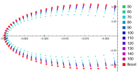
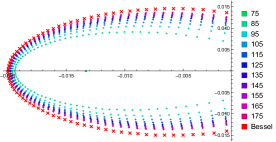
from which it follows that as n+𝑛n\to+\infty, these recurrence relations are close to (3.17). Thus, the polynomials Pk(z)subscript𝑃𝑘𝑧P_{k}(z) approach Bk(z)subscript𝐵𝑘𝑧B_{k}(z) coefficient-wise, and, therefore, on the compact subsets of the complex plane. So for a=1n𝑎1𝑛a=-\dfrac{1}{n}, sufficiently large n𝑛n, and relatively small k𝑘k (comparing with n𝑛n) one can consider the polynomials Pk(z)subscript𝑃𝑘𝑧P_{k}(z) as an approximation of the monic Bessel polynomials Bk(z)subscript𝐵𝑘𝑧B_{k}(z). Thus, we can expect that for a fixed k𝑘k and large n𝑛n the zeroes of Pk(z)subscript𝑃𝑘𝑧P_{k}(z) will approximate zeroes of Bk(z)subscript𝐵𝑘𝑧B_{k}(z), and as k+𝑘k\to+\infty and n+𝑛n\to+\infty with kn0𝑘𝑛0\dfrac{k}{n}\to 0 the zeroes of Pk(z)subscript𝑃𝑘𝑧P_{k}(z) will approach the same curve as the zeroes of Bk(z)subscript𝐵𝑘𝑧B_{k}(z) for k+𝑘k\to+\infty, see [4, 5] and references there. Figures 3.2 and 3.2 show the zeroes of the polynomials B50(z)subscript𝐵50𝑧B_{50}(z) and B75(z)subscript𝐵75𝑧B_{75}(z), respectively, and the zeroes of P50(z)subscript𝑃50𝑧P_{50}(z) and P75(z)subscript𝑃75𝑧P_{75}(z) approaching them as n+𝑛n\to+\infty.

Refer to caption
Figure 3.1. Zeroes of B50subscript𝐵50B_{50} and P50subscript𝑃50P_{50} for n=50,,150𝑛50150n=50,\dots,150
Refer to caption
Figure 3.2. Zeroes of B75subscript𝐵75B_{75} and P75subscript𝑃75P_{75} for n=75,,175𝑛75175n=75,\dots,175

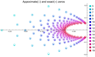
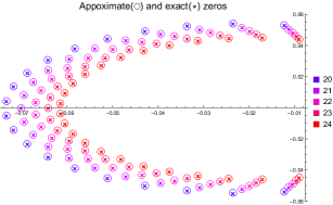
Figures 3.4 and 3.4 represent the zeroes of the polynomials Pk(z)subscript𝑃𝑘𝑧P_{k}(z) and Bk(z)subscript𝐵𝑘𝑧B_{k}(z) for n=k2𝑛superscript𝑘2n=k^{2} and k=5,,24𝑘524k=5,\ldots,24. There is a visibly good approximation of Bk(z)subscript𝐵𝑘𝑧B_{k}(z) by Pk(z)subscript𝑃𝑘𝑧P_{k}(z) in such a case.

Refer to caption
Figure 3.3. Zeroes of Pksubscript𝑃𝑘P_{k} and Bksubscript𝐵𝑘B_{k} for n=k2𝑛superscript𝑘2n=k^{2} and k=5,,19𝑘519k=5,\ldots,19
Refer to caption
Figure 3.4. Zeroes of Pksubscript𝑃𝑘P_{k} and Bksubscript𝐵𝑘B_{k} for n=k2𝑛superscript𝑘2n=k^{2} and k=20,,24𝑘2024k=20,\ldots,24

Note also that if a=1n𝑎1𝑛a=-\dfrac{1}{n}, then as n+𝑛n\to+\infty the limits of the moments sm(n)subscript𝑠𝑚𝑛s_{m}(n), m=0,1,2,𝑚012m=0,1,2,\ldots, are close to the moments of the Bessel polynomials (but not the same). At the same time, the inverse Fourier transform of the distributional weight function corresponding to the Bessel polynomials has the form

F1w(t)=12πk=0+2k+1(it)kk!(k+1)!=I1(8it)π8it,superscript𝐹1𝑤𝑡12𝜋superscriptsubscript𝑘0superscript2𝑘1superscript𝑖𝑡𝑘𝑘𝑘1subscript𝐼18𝑖𝑡𝜋8𝑖𝑡F^{-1}w(t)=-\dfrac{1}{2\pi}\sum\limits_{k=0}^{+\infty}\dfrac{2^{k+1}(it)^{k}}{k!(k+1)!}=-\dfrac{I_{1}(\sqrt{8it})}{\pi\sqrt{8it}},

where I1(x)subscript𝐼1𝑥I_{1}(x) is the modified Bessel function [29].

3.4. Zeroes of polynomials Pk(z)subscript𝑃𝑘𝑧P_{k}(z) for fixed a𝑎a

Apart of approximation of Bessel polynomials, it is interesting to study how the zeroes the polynomials Pksubscript𝑃𝑘P_{k} behave for a fixed a{0}𝑎0a\in\mathbb{C}\setminus\{0\}. As it was already observed in Section 3.1, the results on the polynomials Pksubscript𝑃𝑘P_{k} for a certain fixed a{0}𝑎0a\in\mathbb{C}\setminus\{0\} immediately extend to other values of a𝑎a due to

akPk(az)=Pk(z)|a=1or, equivalently,(a)kPk(az)=Pk(z)|a=1.formulae-sequencesuperscript𝑎𝑘subscript𝑃𝑘𝑎𝑧evaluated-atsubscript𝑃𝑘𝑧𝑎1or, equivalently,superscript𝑎𝑘subscript𝑃𝑘𝑎𝑧evaluated-atsubscript𝑃𝑘𝑧𝑎1a^{-k}P_{k}(az)=P_{k}(z)\big{|}_{a=1}\quad\text{or, equivalently,}\quad(-a)^{-k}P_{k}(-az)=P_{k}(z)\big{|}_{a=-1}.

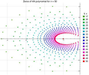
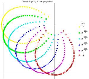
Accordingly, varying values of a𝑎a only scales and/or rotates the zeroes of these polynomials in \mathbb{C}, see Figure 3.6. We shall concentrate on the case a=1𝑎1a=-1 which is related to the previous section.
Refer to caption
Figure 3.5. Zeroes of Pksubscript𝑃𝑘P_{k} for a=eiφ𝑎superscript𝑒𝑖𝜑a=e^{i\varphi} with n=k+1=71𝑛𝑘171n=k+1=71, and φ=π,,π2𝜑𝜋𝜋2\varphi=-\pi,\dots,-\frac{\pi}{2}
Refer to caption
Figure 3.6. Zeroes of Pksubscript𝑃𝑘P_{k} for a=1𝑎1a=-1, k=17,,50𝑘1750k=17,\ldots,50, and n=50𝑛50n=50

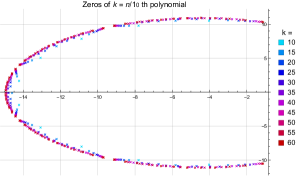
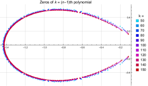
Figures 3.8 and 3.8 represent the zeroes of the polynomials Pn/10(z)subscript𝑃𝑛10𝑧P_{n/10}(z) and Pn1(z)subscript𝑃𝑛1𝑧P_{n-1}(z) for a=1𝑎1a=-1. According to calculations, the zeroes tend to a certain curve in the left half-plane that depends on the limiting ratio kn𝑘𝑛\dfrac{k}{n} as k𝑘k\to\infty, n>k𝑛𝑘n>k.

Refer to caption
Figure 3.7. Zeroes of Pksubscript𝑃𝑘P_{k} for a=1𝑎1a=-1, n=10k𝑛10𝑘n=10k, and k=10,,60𝑘1060k=10,\ldots,60
Refer to caption
Figure 3.8. Zeroes of Pksubscript𝑃𝑘P_{k} for a=1𝑎1a=-1, n=k+1𝑛𝑘1n=k+1, and k=50,,150𝑘50150k=50,\ldots,150

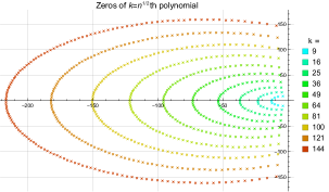
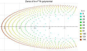
If one changes linear dependence between n𝑛n and k𝑘k to higher powers, the zeroes of Pksubscript𝑃𝑘P_{k} move to infinity as k+𝑘k\to+\infty, see Figures 3.10 and 3.10.

Refer to caption
Figure 3.9. Zeroes of Pksubscript𝑃𝑘P_{k} for a=1𝑎1a=-1, n=k2𝑛superscript𝑘2n=k^{2}, and k=9,,144𝑘9144k=9,\ldots,144
Refer to caption
Figure 3.10. Zeroes of Pksubscript𝑃𝑘P_{k} for a=1𝑎1a=-1, n=k5/4𝑛superscript𝑘54n=\lfloor k^{5/4}\rfloor, and k=9,,144𝑘9144k=9,\ldots,144

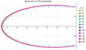
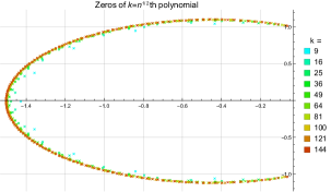
This phenomenon may be explained as follows. As kn0𝑘𝑛0\dfrac{k}{n}\to 0 we can rescale the polynomials Pk(z)subscript𝑃𝑘𝑧P_{k}(z) to have the zeroes bounded. The proper rescaling may be achieved by letting a=1n𝑎1𝑛a=-\dfrac{1}{n} and study the asymptotic behaviour of the zeroes of Pk(zk)subscript𝑃𝑘𝑧𝑘P_{k}\left(\dfrac{z}{k}\right), which is equivalent to letting a=kn𝑎𝑘𝑛a=-\dfrac{k}{n} and studying the zeroes of Pk(z)subscript𝑃𝑘𝑧P_{k}(z), see Figures 3.12 and 3.12. From the discussion in Section 3.3 it follows that the zeroes of Pk(zk)subscript𝑃𝑘𝑧𝑘P_{k}\left(\dfrac{z}{k}\right) for a=1n𝑎1𝑛a=-\dfrac{1}{n} should approximate those of Bk(zk)subscript𝐵𝑘𝑧𝑘B_{k}\left(\dfrac{z}{k}\right) as k𝑘k\to\infty, n𝑛n\to\infty, kn0𝑘𝑛0\dfrac{k}{n}\to 0. At the same time, the latter zeroes are known to remain bounded [19, 30], see also [4, 5].
Refer to caption
Figure 3.11. Zeroes of Pksubscript𝑃𝑘P_{k} for a=k/n𝑎𝑘𝑛a=-k/n, n=k2𝑛superscript𝑘2n=k^{2}, and k=9,,144𝑘9144k=9,\ldots,144
Refer to caption
Figure 3.12. Zeroes of Pksubscript𝑃𝑘P_{k} for a=k/n𝑎𝑘𝑛a=-k/n, n=k5/4𝑛superscript𝑘54n=\lfloor k^{5/4}\rfloor, and k=9,,144𝑘9144k=9,\ldots,144

Acknowledgement

The results of Theorems 2.1 and 2.4, Corollary 2.7 and Sections 3.2 and 3.3 (except Theorem 3.2) were obtained with the support of the Russian Science Foundation grant 19-71-30002. The work on Remarks 2.2 and 2.6, Section 3.1 and all numerical calculations were supported by the state assignment, registration number 122041100132-9.

References

  • [1] M. Alfaro, T.  E. Pérez, M. A. Piñar, M. L. Rezola, Sobolev orthogonal polynomials: the discrete-continuous case, Methods Appl. Anal.,  6, no. 4, 1999, 593–616.
  • [2] G. Baker, Jr. and P. Graves-Morris, Padé approximants, Vol. 1, Encyclopedia of Mathematics and Applications 13, Addison-Wesley Publ. Co., 1980.
  • [3] A. Behn, K. R. Driessel, I. R. Hentzel, K. A. Vander Velden, and J. Wilson, Some nilpotent, tridiagonal matrices with a special sign pattern, Linear Algebra Appl.436, no. 12, 2012, 4446–4450.
  • [4] M.G. de Bruin, E.B. Saff, and R.S Varga, On the generalized Bessel polynomials. I, Indag. Math.84, no. 1, 1981, 1–13.
  • [5] M.G. de Bruin, E.B. Saff, and R.S Varga, On the generalized Bessel polynomials. II, Indag. Math.84, no. 1, 1981, 14–25.
  • [6] M.B. Can, R. Howe, and M. Joyce, Unipotent invariant matrices, Linear Algebra Appl., 439, 2013, 196–210.
  • [7] K. Castillo, C.M. da Fonseca, and J. Petronilho, On Chebyshev polynomials and the inertia of certain matrices, Appl. Math. Comput.467, 2024, no. 128497.
  • [8] V. Černý and J. Hrušák, On some new similarities between non-linear observer and filter design, Nonlinear Control Syst., 6, 2004, 465–470.
  • [9] T.S. Chihara, An Introduction to Orthogonal Polynomials, Gordon and Breach, New York, 1978.
  • [10] M.T. Chu, Inverse eigenvalue problems, SIAM Rev., 40, 1998, 1–39.
  • [11] J.H. Drew, C.R. Johnson, D.D. Olesky, and P. van den Driessche, Spectrally arbitrary patterns, Linear Algebra Appl.308, 2000, 121–137.
  • [12] A.J. Duran, Functions with given moments and weight functions for orthogonal polynomials, Rocky Mountain J. Math., 23, no. 1, 1993, 87–104.
  • [13] L. Elsner and D. Hershkowitz, On the spectra of close-to-Schwarz matrices, Linear Algebra Appl.363, 2003, 81–88.
  • [14] W.D. Evans, W.N. Everitt, K.H.  Kwon, and L.L. Littlejohn, Real orthogonalizing weights for Bessel polynomials, J. Comput. Appl. Math, 49, 1993, 51–57.
  • [15] F.R. Gantmacher, The Theory of Matrices, vol. II, Translated by K. A. Hirsch, Chelsea Publishing Co., New York, 1959.
  • [16] C. Garnett and B. L. Shader, A proof of the conjecture: Centralizers, Jacobians and spectrally arbitrary sign patterns, Linear Algebra Appl.436, no. 12, 2012, 4451–4458.
  • [17] J. Geronimus, Sur les polynômes orthogonaux relatifs à une suite des nombres donnée et sur le théorème de W. Hahn, Izv. Akad. Nauk SSSR, Ser. Mat., 4, no. 2, 1940, 215–228.
  • [18] R. Gragham, D. Knuth, and O. Patashnik, Concrete Mathematics, Advanced Book Program (First ed.), Reading, MA: Addison-Wesley Publ. Co., 1998, pp. xiv+625.
  • [19] E. Grosswald, Bessel polynomials, Lecture Notes in Mathematics, 698, Springer-Verlag, New York, 1978, pp. 182.
  • [20] O. Holtz and M. Tyaglov, Structured matrices, continued fractions, and root localization of polynomials, SIAM Rev., 54, 2012, 421–509.
  • [21] X. Hou, Z. Xiao, Y. Hao, and Q. Yuan, Decomposition of symplectic matrices into products of symplectic unipotent matrices of index 222, Electron. J. Linear Algebra, 35, 2019, 497–502.
  • [22] C.R. Johnson, B.D. Sutton, and A.J. Witt, Implicit construction of multiple eigenvalues for trees, Linear Multilinear Algebra, 57, 2009, 409–420.
  • [23] M.E.H. Ismail, Classical and quantum orthogonal polynomials in one variable, with two chapters by W. Van Assche, with a foreword by R. Askey, Encyclopedia of Mathematics and its Applications 98, Cambridge University Press, Cambridge, 2005.
  • [24] H.L. Krall and O. Frink, A new class of orthogonal polynomials: The Bessel polynomials, Trans. Amer. Math. Soc., 65, 1949, 100–115.
  • [25] M.G. Krein and M.A. Naimark, The method of symmetric and Hermitian forms in the theory of the separation of the roots of algebraic equations, Linear and Multilinear Algebra, 1981, 10, 265–308.
  • [26] L. Lorentzen and H. Waadeland, Continued Fractions with Applications, North-Holland Publishing Co., Amsterdam, 1992.
  • [27] F. Marcellán and R. Álvarez-Nodarse, On the “Favard theorem” and its extensions, J. Comput. Appl. Math, 127, 2001, 231–254.
  • [28] A.W. Mason, Unipotent matrices, modulo elementary matrices, in SL2 over a coordinate ring, J. Algebra, 203, 1998, 134–155.
  • [29] R.D. Morton and A.M. Krall, Distributional weight functions for orthogonal polynomials, SIAM J. Math. Anal., 9, no. 4, 1978, 604–626.
  • [30] F.W.J. Olver, The asymptotic expansions of Bessel functions of large order, Phil. Trans. Roy. Soc. London Ser. A, 247, 1954, 338–368.
  • [31] A. Prudnikov, Yu. Brychkov, and O. Marichev, Integrals and Series, Vol. 1, Elementary functions, Phys. and Math. Literature, Moscow, 2002, p. 632.
  • [32] H.R. Schwarz, Ein Verfahren zur Stabilitätsfrage bei Matrizen-Eigenwertproblemen, Zeitschrift für angew. Math. Phys., 7, no. 6, 1956, 473–500.
  • [33] R.L. Soto, A.I. Julio, and J.H. Alfaro, Permutative universal realizability, Spec. Matrices, 9, 2021, 66–77.
  • [34] B.D. Sutton, Numerical construction of structured matrices with given eigenvalues, Spec. Matrices, 7, 2019, 263–271.
  • [35] M. Tyaglov, Sign patterns of the Schwarz matrices and generalized Hurwitz polynomials, Electron. J. Linear Algebra, 24, 2012, 215–236.
  • [36] H.S. Wall, Polynomials whose zeros have negative real parts, Amer. Math. Monthly, 52, no. 6, 1945, 308–322.
  • [37] H.S. Wall, Analytic Theory of Continued Fractions, D. Van Nostrand Company Inc., New York, 1948.
  • [38] H. Zassenhaus, Characterization of unipotent matrices, J. Number Theory, 1, 1969, 222–230.