Revisiting Cosine Similarity via Normalized ICA-transformed Embeddings

Abstract

Cosine similarity is widely used to measure the similarity between two embeddings, while interpretations based on angle and correlation coefficient are common. In this study, we focus on the interpretable axes of embeddings transformed by Independent Component Analysis (ICA), and propose a novel interpretation of cosine similarity as the sum of semantic similarities over axes. To investigate this, we first show experimentally that unnormalized embeddings contain norm-derived artifacts. We then demonstrate that normalized ICA-transformed embeddings exhibit sparsity, with a few large values in each axis and across embeddings, thereby enhancing interpretability by delineating clear semantic contributions. Finally, to validate our interpretation, we perform retrieval experiments using ideal embeddings with and without specific semantic components.

1 Introduction

Cosine similarity is widely used to measure the similarity between two embeddings Bojanowski et al. (2017); Reimers and Gurevych (2019); Sitikhu et al. (2019) and can be computed efficiently Li and Han (2013); Xia et al. (2015); Gao et al. (2021). For word embeddings, the norm represents the importance of the word and the direction represents the meaning of the word Yokoi et al. (2020); Oyama et al. (2023). Therefore, cosine similarity, which is the inner product of the normalized embeddings, makes sense as word similarity. Studies dealing with cosine tend to focus on the angle Deng et al. (2019); Li and Li (2023) or interpret it as a correlation coefficient van Dongen and Enright (2012).

Figure 1: Heatmaps of 300-dimensional GloVe embeddings transformed by (left) Independent Component Analysis (ICA) and (right) Principal Component Analysis (PCA), with embeddings normalized to unit length following the transformations. We select five specific axes (50th, 100th, etc.) and display the top five words by component values for each axis. For the normalized ICA-transformed embeddings, the maximum component values on the axes are substantial, highlighting significant features, while the remaining values are typically small, resulting in a sparse representation. Conversely, for the normalized PCA-transformed embeddings, even the maximum values are not large, making it difficult to interpret the meanings of the axes.

(a) Normalized ICA-transformed embeddings of ultraviolet and light and their component-wise products.

(b) Normalized PCA-transformed embeddings of ultraviolet and light and their component-wise products.

Figure 2: For the (a) ICA and (b) PCA transformations, bar graphs are displayed for each, plotting the component values of the normalized GloVe embeddings: (left) ultraviolet, (middle) light, and (right) their component-wise products. The axes with the top five component values in the ultraviolet embedding are highlighted, and these same axes are consistently colored across the other two plots. The sum of the component-wise products corresponds to the cosine similarity value of $0.485$ for both transformations. See Table 2 in Appendix B for the top words of the axes. The component [spectrum] of the normalized ICA-transformed embeddings is much more emphasized in the component-wise products than in the components, because their standard deviations are $1/d$ and $1/\sqrt{d}$, respectively. See Appendix B for more descriptions and Appendix C for details of the distribution theory.

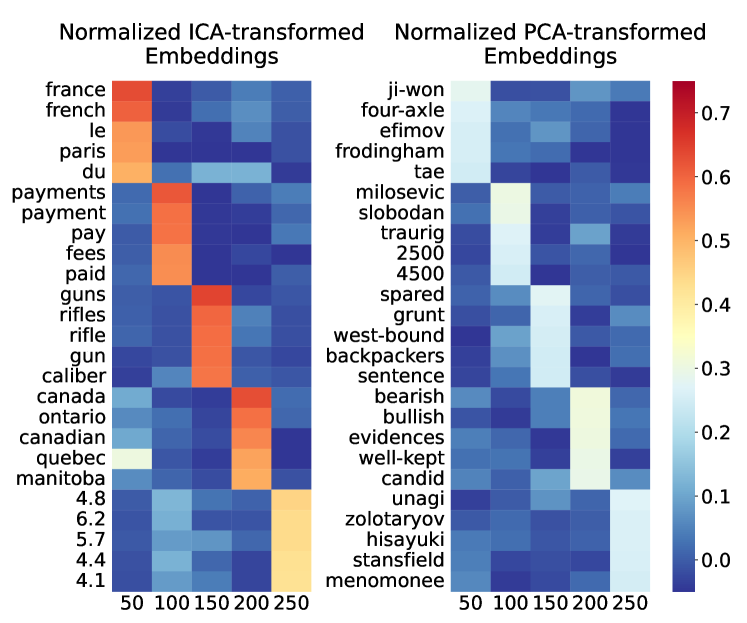
Unlike existing studies, our research introduces a novel interpretation of cosine similarity, focusing on embeddings transformed by Independent Component Analysis (ICA) Hyvärinen and Oja (2000), which aims to maximize the independence of components. To implement the ICA transformation, FastICA Hyvärinen (1999), which is derived from Principal Component Analysis (PCA) Hotelling (1933), is widely used. ICA-transformed embeddings are known to have interpretable axes Mareček et al. (2020); Musil and Mareček (2022); Yamagiwa et al. (2023). Specifically, Yamagiwa et al. (2023) determined the meanings of the axes by examining the top words with the highest component values in the normalized ICA-transformed embeddings. Figure 1 shows heatmaps of the normalized embeddings after ICA and PCA transformations. These axes of the ICA-transformed embeddings can be interpreted as [france], [payments], [guns], [canada], and [decimals], whereas those of the PCA-transformed embeddings remain uninterpretable. Hereafter, the meaning of an axis will be denoted as [decimals] and a word is denoted as paris, with their indices denoted as $\ell_{\text{{[decimals]}}}$ and $i_{\text{{paris}}}$, respectively.

The inner product of normalized embeddings represents the cosine similarity. Figure 2 displays the normalized embeddings transformed by ICA and PCA for ultraviolet and light, along with their component-wise products, shown in a bar graph. The sum of the component-wise products forms the inner product, yielding an identical cosine similarity value of $0.485$ for both transformations. This equivalence arises because the ICA embeddings are obtained by rotating the PCA embeddings. However, a closer examination of the component-wise products shows distinct differences: In the ICA-transformed embeddings, both ultraviolet and light exhibit a large component value in [spectrum], resulting in a significant product value and sparse values elsewhere. Conversely, the PCA-transformed embeddings do not have any axes with large component values, resulting in a uniformly dense vector. These differences illustrate that, while the overall cosine similarity is the same, the underlying structural contributions to this similarity vary significantly between the two transformations.

Based on these observations, we define the semantic similarity of the $\ell$-th axis for words $w_{i}$ and $w_{j}$ as the component-wise product of the normalized ICA-transformed embeddings, denoted as $\text{sem}_{\ell}(w_{i},w_{j})$. For example, in Fig. 2,

$$\text{sem}_{\ell_{\text{{[spectrum]}}}}(\text{{ultraviolet}},\text{{light}})=0.296.$$

Thus, the cosine similarity can be interpreted as the sum of the semantic similarities across all axes:

$$\cos(w_{i},w_{j})=\sum_{\ell=1}^{d}\text{sem}_{\ell}(w_{i},w_{j}),$$ (1)

which represents the “additive compositionality” of semantic similarities, decomposing overall similarity into the component-wise similarities.

In this study, we aim to explore the interpretation of the cosine similarity presented in (1). First, we explain the PCA and ICA transformations for embeddings. Next, we consider the need for normalization and demonstrate in Fig. 3 that unnormalized embeddings contain norm-derived artifacts. We then compare ICA and PCA, showing in Fig. 4 that for normalized ICA-transformed embeddings, a few large component values tend to be present in each axis and across embeddings. Finally, we give an explanation of (1) and, based on this interpretation, perform experiments on ideal embeddings and downstream tasks.

2 Related work

2.1 Cosine similarity

Cosine similarity is commonly used to measure the similarity between two embeddings, such as word Mikolov et al. (2013b, c); Pennington et al. (2014), token Zhang et al. (2020); Bommasani et al. (2020), and sentence embeddings Reimers and Gurevych (2019); Gao et al. (2021). Cross-lingual alignment methods based on cosine similarity have also been proposed Xing et al. (2015); Alvarez-Melis and Jaakkola (2018); Lample et al. (2018).

There are studies that question the effectiveness of cosine similarity. For example, Schnabel et al. (2015) showed that word frequency can affect cosine similarity. Steck et al. (2024) used linear models to show cases where cosine similarity fails.

(c) Before Normalization

(d) After Normalization

Figure 3: Scatterplots for the 150th axis of the ICA-transformed embeddings, (a) before and (b) after normalization, showing the ranks of component values within the axis and within each embedding, colored by the norms. The larger the norm of an embedding, the more it is plotted in the foreground. See Appendix A for other axes and the PCA-transformed embeddings.

(a) Each Axis

(b) Each Embedding

Figure 4: Comparison of component values of normalized embeddings following ICA and PCA transformations. The component values are sorted in descending order for (a) each axis and (b) each embedding, and their averages are plotted. The range of $\pm 1\sigma$ is shown, where $\sigma$ is the standard deviation of the component values.

2.2 Interpretability of embeddings

Research on the interpretability of embeddings has used various methods, including non-negative matrix factorization Murphy et al. (2012), sparse coding Faruqui et al. (2015), methods for learning interpretable embeddings Luo et al. (2015); Sun et al. (2016), rotation of embeddings Park et al. (2017), Singular Value Decomposition (SVD)  Shin et al. (2018), autoencoders Subramanian et al. (2018); Huben et al. (2024), and PCA Musil (2019).

There has also been a lot of research on applying ICA to embeddings. For example, Chagnaa et al. (2007) showed that the features of similar verbs have a large same independent component through bar graphs. The axes of the ICA-transformed embeddings are known to be interpretable Mareček et al. (2020); Musil and Mareček (2022). Moreover, such axes are also observed in embeddings for other languages, dynamic models, and images Yamagiwa et al. (2023). Yamagiwa et al. (2024) maximized the semantic continuity of the axes by finding their optimal order.

To invert the meaning of a word, Ishibashi et al. (2020) mirrored the embedding by a hyerplane, while in Section 7.4 we invert the meaning by simply removing the component from a particular axis.

2.3 Norm of word embedding

Studies have shown that the norm of word embeddings contains information about the word. For example, tokens with less information tend to have smaller norms Schakel and Wilson (2015); Pagliardini et al. (2018); Arefyev et al. (2018); Kobayashi et al. (2020) and BERT embeddings show a negative correlation between word frequency and norm Liang et al. (2021). Oyama et al. (2023) showed that the squared norm of an embedding can approximate the Kullback-Leibler (KL) divergence, and Kurita et al. (2023) found a correlation between KL and Integrated Gradients Sundararajan et al. (2017) in contrastive-based sentence encoders. Yokoi et al. (2020) proposed norm-proportional weights for optimal transport. Nagata et al. (2023) considered the norm of the mean vector of normalized embeddings as the degree of semantic breadth.

3 Background

In this section, we explain PCA and ICA transformations for embeddings based on Yamagiwa et al. (2023). Let $\mathbf{X}\in\mathbb{R}^{n\times d}$ be pre-trained embeddings with vocabulary size $n$ and dimension $d$. We assume that $\mathbf{X}$ is centered, i.e., the mean of each column is zero.

3.1 PCA-transformed embeddings

PCA, typically implemented using algorithms such as SVD, transforms the embeddings so that their components align with the directions of maximum variance. The PCA-transformed embeddings $\mathbf{Z}\in\mathbb{R}^{n\times d}$ of $\mathbf{X}$ are given by the transformation matrix $\mathbf{A}\in\mathbb{R}^{d\times d}$ as

$$\mathbf{Z}=\mathbf{X}\mathbf{A}.$$ (2)

The columns of $\mathbf{Z}$ are called principal components (PC), and the matrix $\mathbf{Z}$ is whitened; i.e., the variance of each column is $1$ and the columns are uncorrelated with each other. Whitening generally improves the quality of the embeddings Su et al. (2021); Sasaki et al. (2023).

3.2 ICA-transformed embeddings

ICA transforms the embeddings so that their components are as independent as possible. The ICA-transformed embeddings $\mathbf{S}\in\mathbb{R}^{d\times d}$ of $\mathbf{X}$ are given by the transformation matrix $\mathbf{B}\in\mathbb{R}^{d\times d}$ as

$$\mathbf{S}=\mathbf{X}\mathbf{B}.$$ (3)

The columns of $\mathbf{S}$ are called independent components (IC).

In particular, FastICA Hyvärinen (1999) uses $\mathbf{Z}$ in (2) to compute $\mathbf{S}$ as follows:

$$\mathbf{S}=\mathbf{Z}\mathbf{R}_{\text{ica}},$$ (4)

where $\mathbf{R}_{\text{ica}}\in\mathbb{R}^{d\times d}$ is an orthogonal matrix that maximizes the statistical independence of the columns of $\mathbf{S}$. Similar to $\mathbf{Z}$, the matrix $\mathbf{S}$ is also whitened.

In this study, following Yamagiwa et al. (2024), we use $300$-dimensional GloVe Pennington et al. (2014) with $n=400{,}000$ and run FastICA from scikit-learn Pedregosa et al. (2011) as the ICA transformation for the embeddings, setting iterations to $10{,}000$ and tolerance to $10^{-10}$ as the hyperparameters for the transformation. Similar to Yamagiwa et al. (2023), we flip the signs of the axes in $\mathbf{S}$ if necessary to ensure positive skewness, and sort the axes in descending order of their skewness.

4 Normalization of embeddings

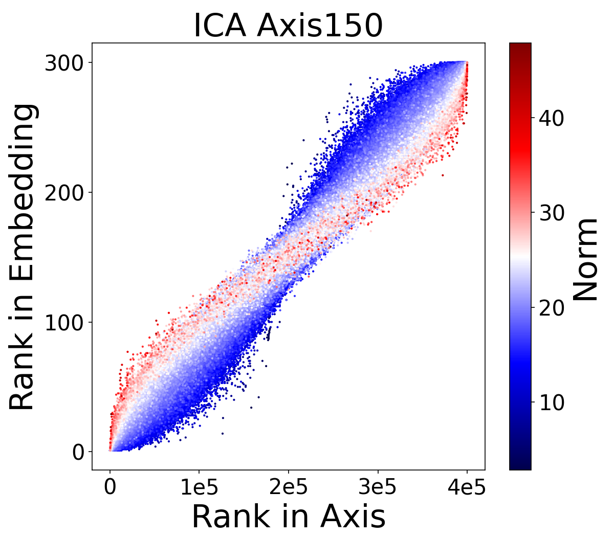
As seen in Fig. 1, while the meanings of the axes of the ICA-transformed embeddings can be interpreted from the top words, the ranks of the component values within each axis can change before and after normalization. Thus, we compare the ranks of the values within each axis and within each embedding, both before and after normalization.

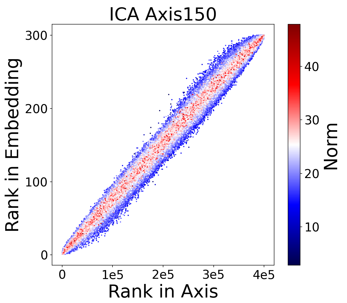
Figure 3 shows the ranks for the $150$th axis. Before normalization, as shown in Fig. 3, embeddings with higher ranks within the axis tend to have lower ranks within each embedding as their norms increase. After normalization, as shown in Fig. 3, the norm-derived artifacts observed in Fig. 3 disappear. These results are consistent with existing research Yokoi et al. (2020); Oyama et al. (2023), suggesting that the direction of a word embedding, independent of the norm, represents the meaning of the word. Similar results are observed in other axes, the PCA-transformed embeddings, and other embeddings, as discussed in Appendix A.

5 Comparison of ICA and PCA

As seen in (4), the ICA-transformed embeddings are orthogonal transformations of the PCA-transformed embeddings; however, the component values of these embeddings can differ significantly. This also applies to their normalized embeddings, so we compare the component values of these normalized embeddings.

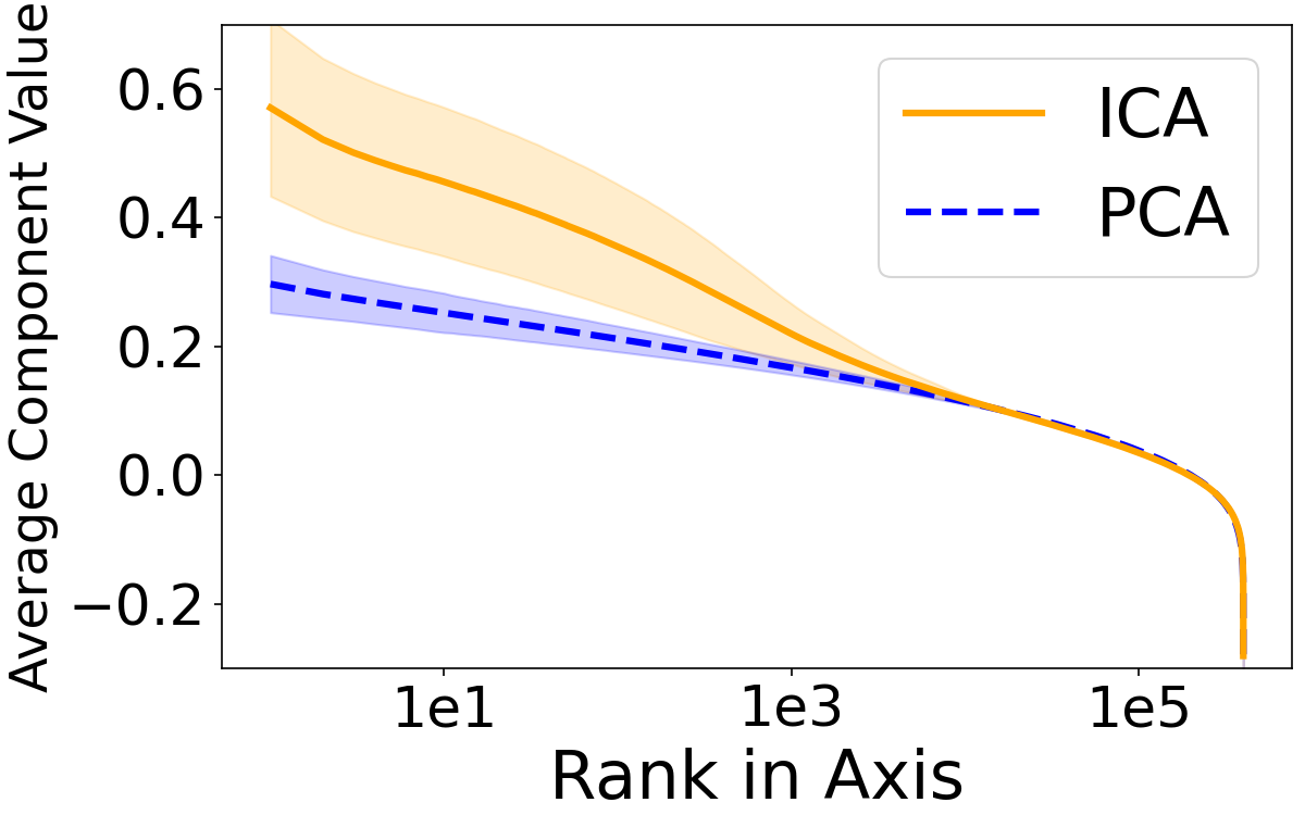
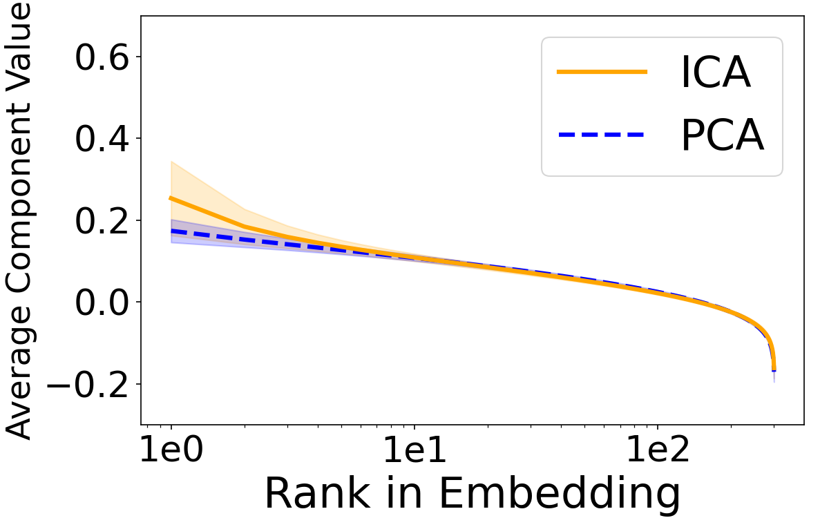
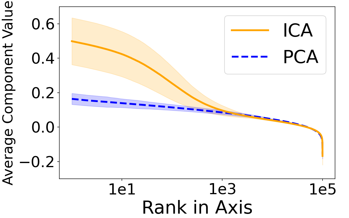
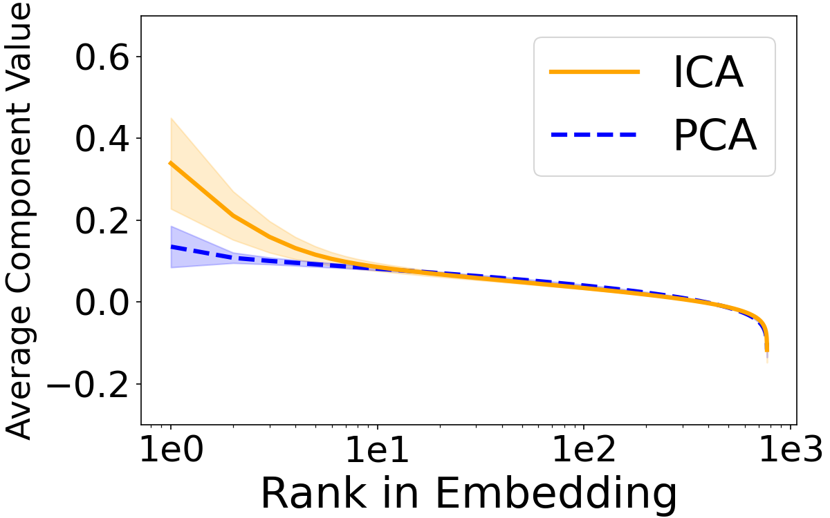
Figure 4 shows a plot of the component values for each axis, sorted in descending order and averaged. The values for ICA are larger than those for PCA up to about the $10{,}000$th axis. This indicates that an axis of the normalized ICA-transformed embeddings contains a greater number of components with larger values than that of the normalized PCA-transformed embeddings. Figure 4 shows a plot of the component values for each embedding, sorted in descending order and averaged. The values for ICA are larger than those for PCA up to about the $10$th axis. This indicates that in a normalized ICA-transformed embedding, there are several axes with larger component values than in a normalized PCA-transformed embedding.

These results suggest that in normalized ICA-transformed embeddings, large component values tend to be present in each axis and embedding.

6 Interpretation

Figure 5: Cosine similarity interpretation. For the normalized ICA-transformed embedding of ultraviolet, the meanings of the axes of the top five components are [chemistry], [biology], [space], [spectrum], and [virology]. For the top words on these axes, see Table 2 in Appendix B. The cosine similarities are calculated between ultraviolet and the top words on these axes: salts, proteins, spacecraft, light, and virus, respectively. The inner products (i.e., cosine similarities) of their normalized ICA-transformed embeddings are computed, and the semantic similarities of these five axes are displayed. For example, the semantic similarity of the [space] axis between ultraviolet and spacecraft is $0.155$, which is more than half of the cosine similarity of $0.260$. The value of [space] in the distribution of semantic similarity is much more emphasized than the value of $\cos(\textrm{ultraviolet},\textrm{spacecraft})$ in the distribution of cosine similarity because their standard deviations are $1/d$ and $1/\sqrt{d}$, respectively. See Appendix B for more descriptions and Appendix C for details of the distribution theory.

6.1 Normalized ICA-transformed embeddings

The ICA-transformed embedding of a word $w_{i}$, denoted by $\mathbf{s}_{i}\in\mathbb{R}^{d}$, is normalized to $\hat{\mathbf{s}}_{i}\in\mathbb{R}^{d}$:

$$\hat{\mathbf{s}}_{i}:=\mathbf{s}_{i}/\|\mathbf{s}_{i}\|=(\hat{s}_{i}^{(1)},\ldots,\hat{s}_{i}^{(\ell)},\ldots,\hat{s}_{i}^{(d)}).$$ (5)

Based on Sections 4 and 5, $\hat{s}_{i}^{(\ell)}$ can be interpreted as the semantic component of the word $w_{i}$ on the $\ell$-th axis. For example, as shown in Fig. 2(a), the normalized ICA-transformed embedding of ultraviolet has large semantic components of [chemistry], [biology], [space], [spectrum], and [virology].

6.2 Cosine similarity

Cosine similarity is widely used to measure the similarity between words. The cosine similarity between words $w_{i}$ and $w_{j}$ can be expressed as the inner product of their normalized ICA-transformed embeddings $\hat{\mathbf{s}}_{i}$ and $\hat{\mathbf{s}}_{j}$:

$$\cos(w_{i},w_{j})=\hat{\mathbf{s}}_{i}^{\top}\hat{\mathbf{s}}_{j}=\sum_{\ell=1}^{d}\hat{s}_{i}^{(\ell)}\hat{s}_{j}^{(\ell)}.$$ (6)

As seen in Section 6.1, $\hat{s}_{i}^{(\ell)}$ can be interpreted as the semantic component of a word $w_{i}$ on the $\ell$-th axis. Therefore, the semantic similarity for words $w_{i}$ and $w_{j}$ on the $\ell$-th axis, $\text{sem}_{\ell}(w_{i},w_{j})$, is defined as:

$$\text{sem}_{\ell}(w_{i},w_{j}):=\hat{s}_{i}^{(\ell)}\hat{s}_{j}^{(\ell)}.$$ (7)

Using (7), the expression for the cosine similarity in (6) can be rewritten as in (1). Thus, the cosine similarity can be interpreted as the sum of the semantic similarities over all axes.

Note that the cosine similarity between two embeddings is the same for the ICA-transformed embeddings and the PCA-transformed embeddings, while it differs from the original cosine similarity before these transformations. As seen in (4), since $\mathbf{S}$ is $\mathbf{Z}$ multiplied by the orthogonal matrix $\mathbf{R}_{\text{ica}}$, $\hat{\mathbf{z}}_{i}=\mathbf{R}_{\text{ica}}\hat{\mathbf{s}}_{i}$, where $\hat{\mathbf{z}}_{i}$ is the normalized PCA-transformed embedding of $w_{i}$. Then $\hat{\mathbf{z}}_{i}^{\top}\hat{\mathbf{z}}_{j}=\hat{\mathbf{s}}_{i}^{\top}\hat{\mathbf{s}}_{j}=\cos(w_{i},w_{j})$.

Figure 6: Bar graphs of the normalized ICA-transformed embeddings for shore_0, shore_1, and shore_2. The ten axes whose component values are large for these shore are interpreted and colored. While shore_0 is a verb, shore_1 and shore_2 are nouns. For the top words of the axes and the sentences containing each shore, see Appendix D.

Figure 7: Performance comparison of ICA and PCA when reducing non-zero normalized component-wise products and then computing cosine similarity. Each value represents the average of $8$ word similarity tasks or $30$ analogy tasks. See Appendix G for more details.

Figure 8: Search results for seven ideal embeddings containing only the semantic components of [food], [animals], and [plants]. For each embedding, the top $10$ words and their cosine similarities are displayed. The search is performed sequentially from top to bottom for each combination of semantic components. Each word has its rank and is assigned a color corresponding to the combination of semantic components where it first appears.

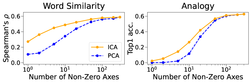
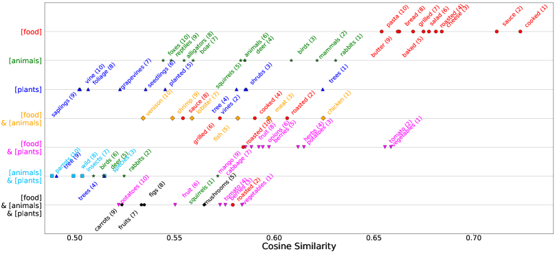
Fig. 2 shows bar graphs for the normalized ICA-transformed and PCA-transformed embeddings of ultraviolet and light and their component-wise products. The sum of the component-wise products is equal to the cosine similarity value ($0.485$) for both transformations. In the normalized ICA-transformed embeddings, the semantic components of [spectrum] are large ($0.535$ for ultraviolet and $0.554$ for light), and the semantic similarity is $\text{sem}_{\ell_{\text{{[spectrum]}}}}(\textit{ultraviolet},\textit{light})=0.296$. Other semantic similarities are close to zero. However, in the normalized PCA-transformed embeddings, although no axis has a component-wise product as large as in the normalized ICA-transformed embeddings, the sum of the component-wise products is still equal to the cosine similarity. Therefore, the component-wise products are not close to zero compared to ICA, resulting in a dense vector.

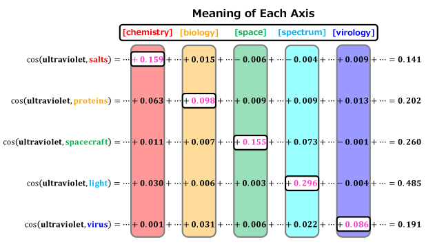
Fig. 5 shows the cosine similarity calculations for ultraviolet with salts, proteins, spacecraft, light, and virus, and semantic similarities for the axes of [chemistry], [biology], [space], [spectrum], and [virology]. The cosine similarity values, which is the sum of the all semantic similarities, can be interpreted from these semantic similarity values.

7 Experiments

7.1 Other embeddings

While we have used the static embedding GloVe to illustrate our interpretation, the use of dynamic embeddings is common in recent large-scale language models. Therefore, we use a simple example to show that ICA transformations are also useful for dynamic embeddings. Yamagiwa et al. (2023) observed that the noun shore has a large component value of [sea], while that of the verb shore is small. We then use their embeddings to examine the semantic components across all axes.

Figure 6 shows the normalized ICA-transformed embeddings of these three shore as bar graphs. For the embeddings of shore_1 and shore_2, the semantic components of [sea] and [location] are large. For the embedding of shore_0, these are small, but those of [cotrol] and [causative verbs] are large. These results explain the large and small relations in the cosine similarity: $\cos(\text{{shore\_1}},\text{{shore\_2}})=0.299$, while $\cos(\text{{shore\_0}},\text{{shore\_1}})=0.054$ and $\cos(\text{{shore\_0}},\text{{shore\_2}})=0.128$. Appendix E shows the ICA transformation in other languages.

7.2 Sparsity of normalized component-wise products for ICA and PCA

We investigate whether the sparsity of component-wise products observed in Fig. 2 also holds for other words. To do this, we perform word similarity and analogy tasks, comparing ICA-transformed and PCA-transformed embeddings. We assess the performance degradation when component-wise products are replaced by zero in ascending order until only $p$ non-zero products remain. Similar to Yamagiwa et al. (2024), we use the Word Embedding Benchmark Jastrzebski et al. (2017).

Figure 7 shows the results for several dimensions. In both tasks, the ICA-transformed embeddings outperform the PCA-transformed embeddings, even when the number of non-zero products is small. The difference in performance between the tasks can be attributed to the fact that in the word similarity task, cosine similarities are computed directly from the word embeddings, whereas in the analogy task, embeddings are added and subtracted before cosine similarities are computed.

7.3 Ideal embeddings with some components

7.3.1 Setting

We define ideal embeddings with specific semantic components and examine words whose normalized ICA-transformed embeddings are close to these ideal embeddings. The ideal embedding $\hat{\mathbf{q}}=(\hat{q}^{(\ell)})_{\ell=1}^{d}\in\mathbb{R}^{d}$ with the semantic components at indices $\ell_{1},\ldots,\ell_{m}$ is defined as follows:

$$\hat{q}^{(\ell)}:=\begin{cases}1/\sqrt{m}&\text{if }\ell={\ell_{1},\ldots,\ell_{m}}\\ 0&\text{otherwise},\end{cases}$$ (8)

where $\|\hat{\mathbf{q}}\|=1$. Note that searching using an ideal embedding with only one semantic component is the same as examining the top words of the axis of the normalized ICA-transformed embeddings. Using the ideal embedding $\hat{\mathbf{q}}$, we search for the top $k$ words by the inner product, i.e., cosine similarity:

$$\mathop{\operatorname{argmax}}_{i\in\llbracket n\rrbracket}{}_{k}\,\hat{\mathbf{q}}^{\top}\hat{\mathbf{s}}_{i},$$ (9)

where $\llbracket n\rrbracket:=\{1,\ldots,n\}$.

7.3.2 Specific examples

As an example, searches using ideal embeddings with the semantic components of [food], [animals], and [plants] yield insightful results. Figure 8 shows these results. The results for one semantic component show that the meanings of the selected axes represent [food], [animals], and [plants]. For the combinations of two semantic components, top words include chicken, meat, and fish for [food] & [animals]; vegetables, tomato, and potatoes for [food] & [plants]; and species, insects, and wild for [animals] & [plants]. In addition, for [food] & [animals] & [plants], top words include words such as mushrooms, fruits, and figs, which are plant-based food favored by animals. As the number of semantic components increases, the ambiguity increases, resulting in lower cosine similarity values.

These results are consistent with an existing study showing that the axes of ICA-transformed embeddings have additive compositional properties and good sparsity Yamagiwa et al. (2023). Moreover, from our perspective, this suggests that word similarity can be well measured by the sum of only a few semantic similarities.

7.4 Ablation of a semantic component

7.4.1 Setting

By setting the $\ell_{\ast}$-th semantic component to zero, we define the ideal embedding for the normalized ICA-transformed embedding of the $i_{\ast}$-th word as

$$\hat{\mathbf{s}}_{i_{\ast}\ominus\ell_{\ast}}:=(\hat{s}_{i_{\ast}}^{(1)},\ldots,\hat{s}_{i_{\ast}}^{(\ell_{\ast}-1)},0,\hat{s}_{i_{\ast}}^{(\ell_{\ast}+1)}\ldots,\hat{s}_{i_{\ast}}^{(d)}).$$ (10)

Since $\|\hat{\mathbf{s}}_{i_{\ast}}\|=1$, it follows that $\|\hat{\mathbf{s}}_{i_{\ast}\ominus\ell_{\ast}}\|\leq 1$. For $\hat{\mathbf{s}}_{i_{\ast}}$ and $\hat{\mathbf{s}}_{i_{\ast}\ominus\ell_{\ast}}$, based on (6), we search for the top $k$ words by their inner products as follows:

$$\mathop{\operatorname{argmax}}_{i\in\llbracket n\rrbracket\setminus\{i_{\ast}\}}{}_{k}\,\hat{\mathbf{s}}_{i_{\ast}}{}^{\top}\hat{\mathbf{s}}_{i},\,\mathop{\operatorname{argmax}}_{i\in\llbracket n\rrbracket\setminus\{i_{\ast}\}}{}_{k}\,\hat{\mathbf{s}}_{i_{\ast}\ominus\ell_{\ast}}{}^{\top}\hat{\mathbf{s}}_{i}.$$ (11)

Note that the original $i_{\ast}$-th word is excluded from the candidates.

7.4.2 Specific examples

$w_{i}$	M	F	$\hat{\mathbf{s}}_{i_{\text{{woman}}}}{}^{\top}\hat{\mathbf{s}}_{i}$	$\hat{\mathbf{s}}_{i_{\text{{woman}}}\ominus\ell_{\text{[female]}}}{}^{\top}\hat{\mathbf{s}}_{i}$
girl		✓	$0.691$	0.595 ($\downarrow 0.096$)
man	✓		$0.679$	0.720 ($\uparrow 0.041$)
mother		✓	$0.632$	0.467 ($\downarrow 0.165$)
person	✓	✓	$0.579$	0.576 ($\downarrow 0.003$)
female		✓	$0.575$	0.518 ($\downarrow 0.057$)
she		✓	$0.568$	0.422 ($\downarrow 0.146$)
herself		✓	$0.567$	0.429 ($\downarrow 0.138$)
wife		✓	$0.553$	0.392 ($\downarrow 0.161$)
women		✓	$0.544$	0.468 ($\downarrow 0.076$)
daughter		✓	$0.535$	0.382 ($\downarrow 0.153$)

Table 1: For the top $10$ words of woman, their inner product values with both woman and woman$\ominus$[female] are shown. Check marks indicate whether words are masculine (M) or feminine (F). The differences between the results for woman and woman$\ominus$[female] are indicated with $\uparrow$ for increases and $\downarrow$ for decreases.

(a) woman and girl

(b) woman and man

Figure 9: Scatterplots of component values of normalized ICA-transformed embeddings for (a) the pair woman and girl and (b) the pair woman and man. The semantic component of [female] is marked with $\blacksquare$ and others with $\bullet$. Figure 21 in Appendix F shows bar graphs for each embedding.

Figure 10: Scatterplot of $\hat{\mathbf{s}}_{i_{\textit{woman}}\ominus\ell_{\textit{[female]}}}{}^{\top}\hat{\mathbf{s}}_{i}$ and $\hat{s}_{i}^{(\ell_{\textit{[female]}})}$ for each $i\in\llbracket n\rrbracket$. The position of woman is marked with $\star$. Words that appear in the top 10 for both woman and woman$\ominus$[female] are marked with $\blacklozenge$, those that appear in the top 10 for woman only with $\blacktriangle$, those that appear in the top 10 for woman$\ominus$[female] only with $\blacktriangledown$, and others with $\bullet$. The value of $\hat{\mathbf{s}}_{i_{\textit{woman}}}{}^{\top}\hat{\mathbf{s}}_{i}$, which represents the cosine similarity $\cos{(\textit{woman},w_{i})}$ between woman and the word $w_{i}$, is plotted as contours. The contour for the 10th closest word daughter to woman is shown as a dash-dotted line. For the 10th closest word women to woman$\ominus$[female], their inner product $\hat{\mathbf{s}}_{i_{\textit{woman}}\ominus\ell_{\textit{[female]}}}{}^{\top}\hat{\mathbf{s}}_{i_{\textit{women}}}$ is shown as a dashed line.

As an example, consider the ablation of a semantic component in the normalized ICA-transformed embedding of woman. We focused on one of the axes with large component values in the embedding, where the top $5$ words were her, wife, mother, daughter, and actress. So we interpret the meaning of this axis as [female]. We then set the semantic component of [female] in the embedding to zero and define an ideal embedding. We call the corresponding ideal word for this ideal embedding woman$\ominus$[female].

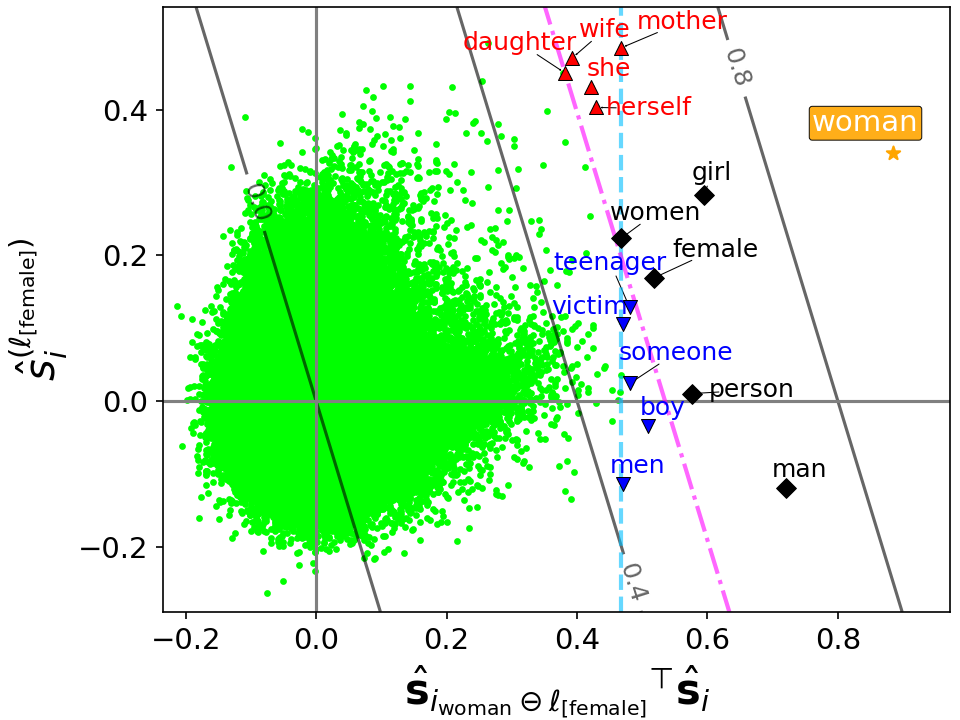
Based on (11), we first searched for the top $10$ words of woman, and then Table 1 shows their inner product values with both woman and woman$\ominus$[female]. Words such as mother, wife, and daughter, which have high inner product values with woman, have lower values with woman$\ominus$[female]. Conversely, man has higher values with woman$\ominus$[female] than with woman.

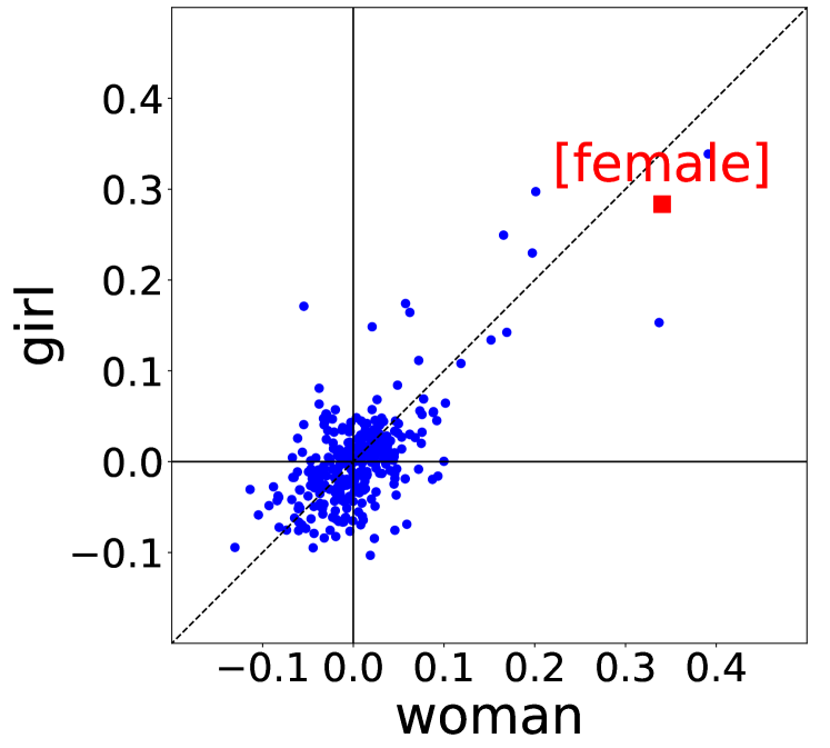
Focusing on girl and man as the top words, Fig. 9 shows scatterplots of the normalized ICA-transformed embeddings for woman and girl, and woman and man. For the semantic component of [female], both the embeddings of woman and girl have positive values, while the embedding of man has negative values. In addition, other semantic components are roughly correlated in both pairs.

7.4.3 Consideration of top word changes

We examine the changes in the top words before and after eliminating the semantic component of [female]. Figure 10 shows a scatterplot of the inner product with woman$\ominus$[female] and the semantic component of [female] for every word. Words in the upper right are close to woman, while those with higher values on the horizontal axis are closer to woman$\ominus$[female]. The transition from dash-dotted to dashed lines indicates that the ablation for [female] replaces the top words for woman such as mother, she, herself, wife, and daughter with the top words for woman$\ominus$[female] such as boy, someone, teenager, men, and victim. These results show that setting one semantic similarity to zero can significantly alter the cosine similarity in (1).

8 Discussion and conclusion

In Section 7.2, we examined the sparsity of the component-wise products of the normalized ICA-transformed embeddings. Based on this, in Sections 7.3 and 7.4, we defined the ideal embeddings with and without specific semantic components. We then searched for close words by the inner products in (6), i.e., cosine similarity, and found that the results were significantly influenced by specific semantic components. This supports our interpretation of cosine similarity as seen in (1).

In summary, we proposed and experimentally validated a new interpretation of cosine similarity. Specifically, we focused on the semantic interpretation of the axes of ICA-transformed embeddings and showed that cosine similarity can be interpreted as the sum of semantic similarities over all axes.

Limitations

• This study explains the interpretation of cosine similarity using centered and whitened embeddings. These embeddings are different from the original embeddings.

• The meanings of the axes of the ICA-transformed embeddings are manually interpreted based on their top words after normalization. In addition, it is not always possible to interpret the meaning of an axis from its top words. Note that the top words used to interpret the meanings of the axes in this study can all be found in the Appendix sections.

• We need to pay attention to the signs of the axes of the ICA-transformed embeddings. In this study, following Yamagiwa et al. (2023), we ensure that all axes have positive skewness by flipping their signs when necessary. We then assume that larger component values are more representative of the meanings of the axes. However, we do not assume that negative component values, whose absolute values are large, represent the opposite meanings of the axes. Therefore, we set $\hat{s}_{i_{\ast}}^{(\ell_{\ast})}$ to $0$ instead of $-\hat{s}_{i_{\ast}}^{(\ell_{\ast})}$ in (10).

• The examples using specific words in Section 7 may have a selection bias. To mitigate this concern, we conducted the experiments to investigate sparsity of normalized component-wise products through the downstream tasks in Section 7.2.

• To explain our interpretation of cosine similarity, we mainly use the GloVe embeddings for which cosine similarity works well. Although cosine similarity may not be effective for all embeddings Steck et al. (2024), this study does not cover which specific types of embeddings are suitable for cosine similarity.

Ethics Statement

This study complies with the ACL Ethics Policy.

Appendix A Additional experiments on normalization of embedding

(a) Each Axis

(b) Each Embedding

Figure 11: Comparison of component values of normalized BERT embeddings following ICA and PCA transformations. The component values are sorted in descending order for (a) each axis and (b) each embedding, and their averages are plotted. The range of $\pm 1\sigma$ is shown, where $\sigma$ is the standard deviation of the component values.

A.1 Rank comparison of component values

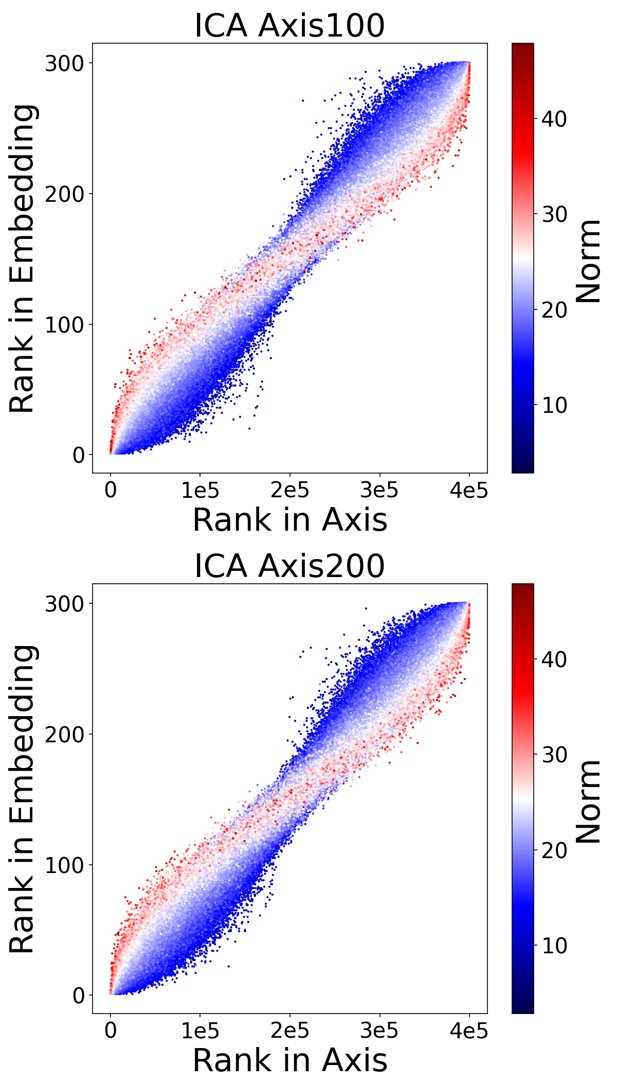
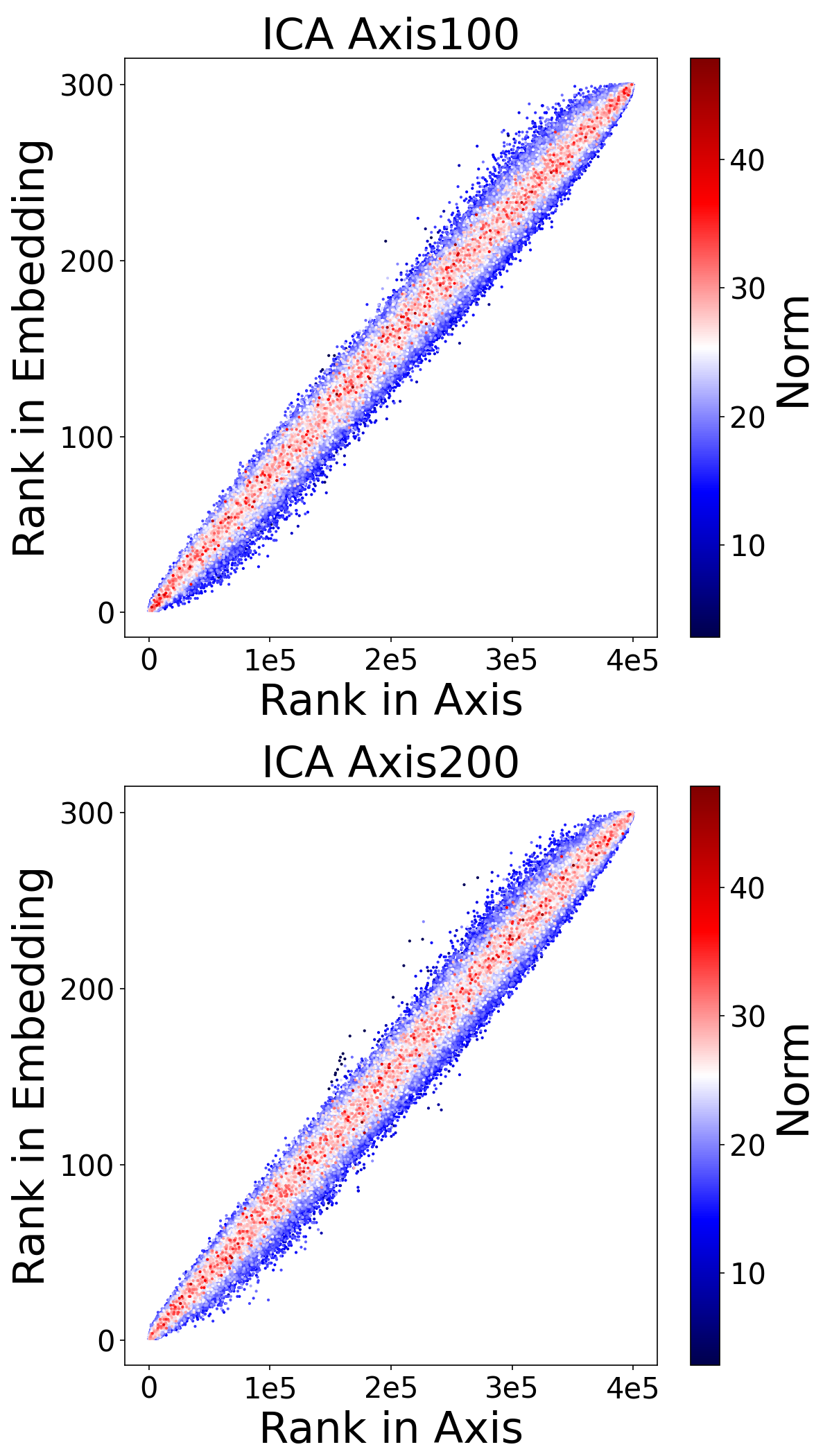
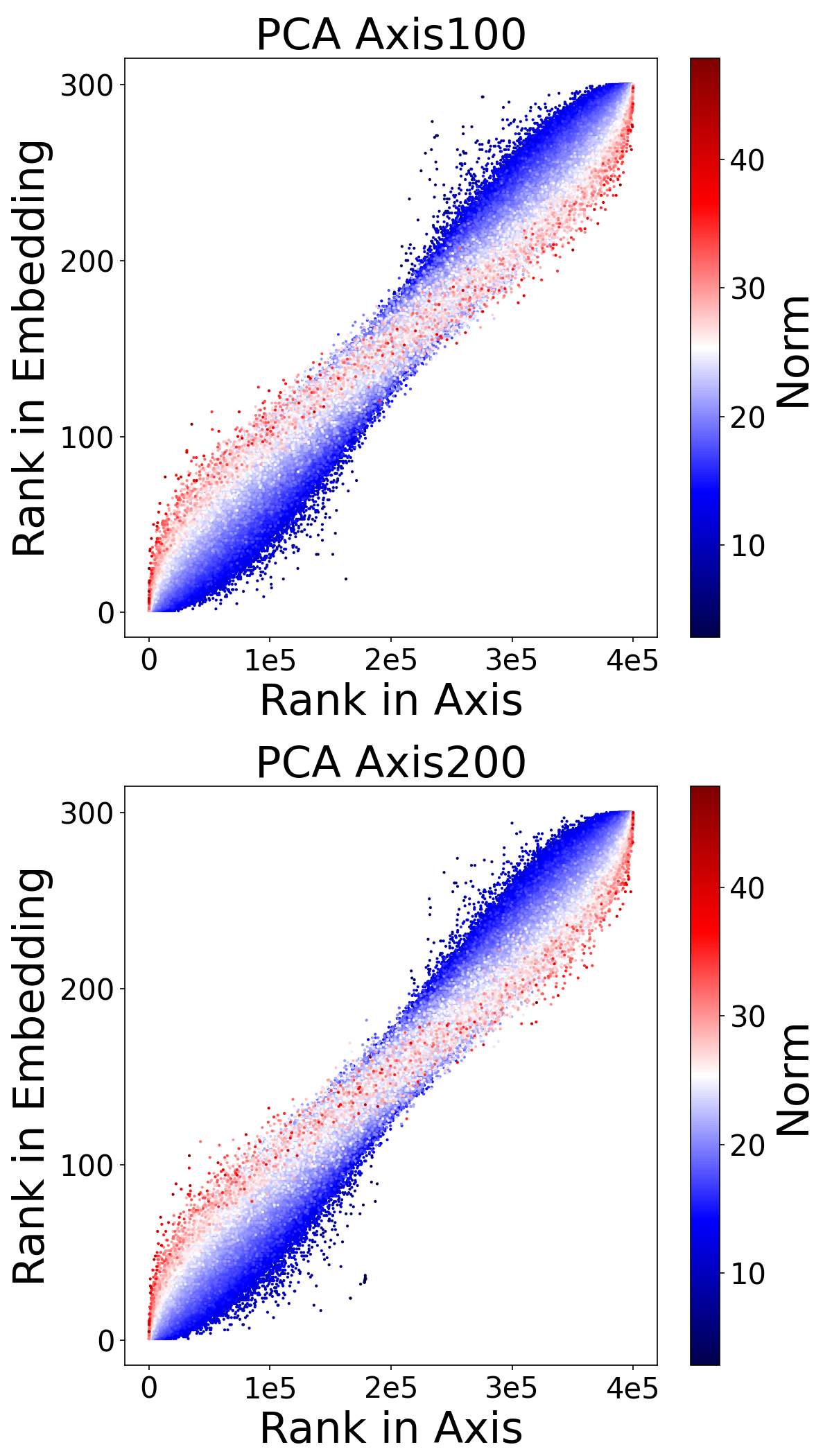
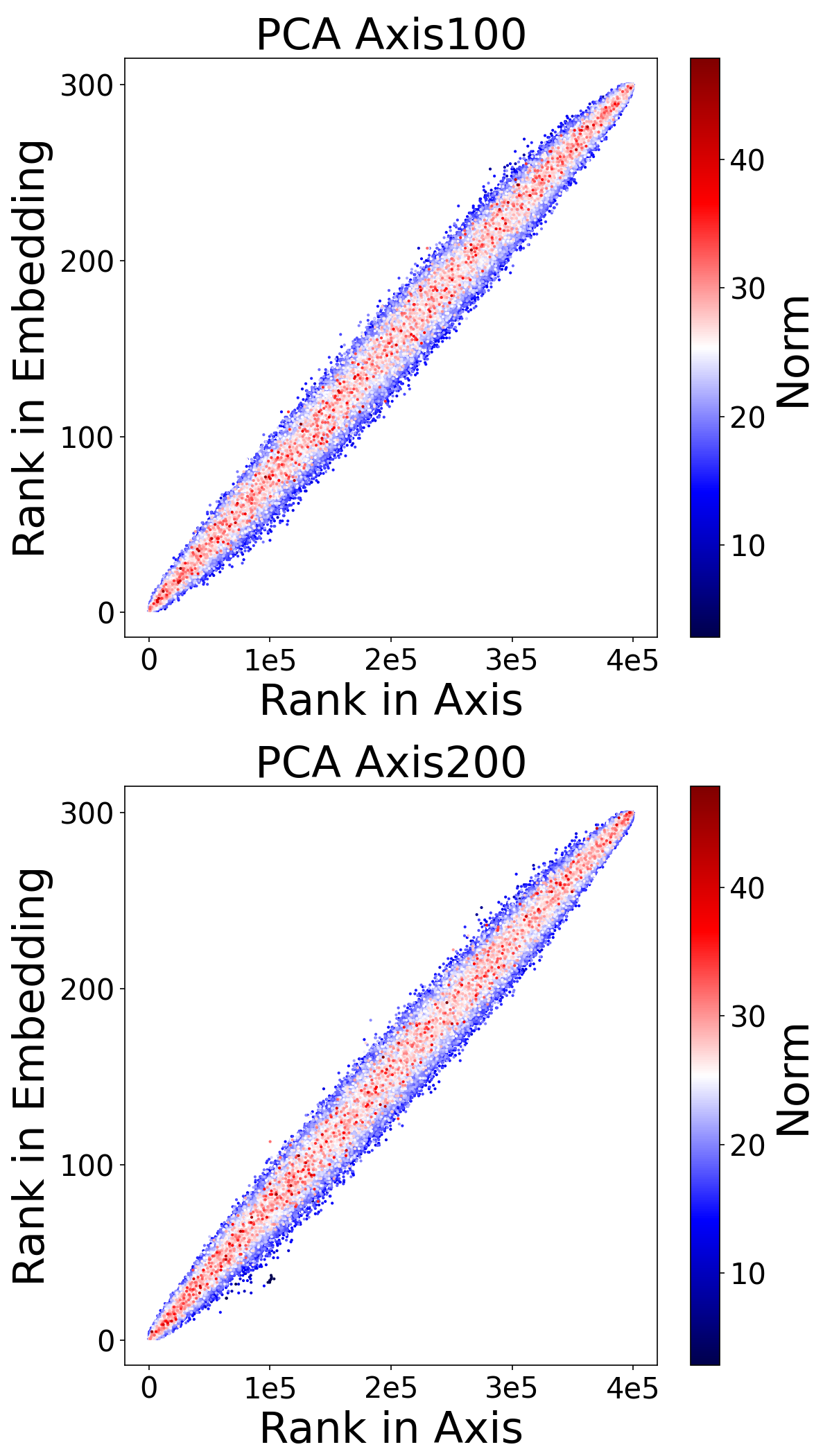
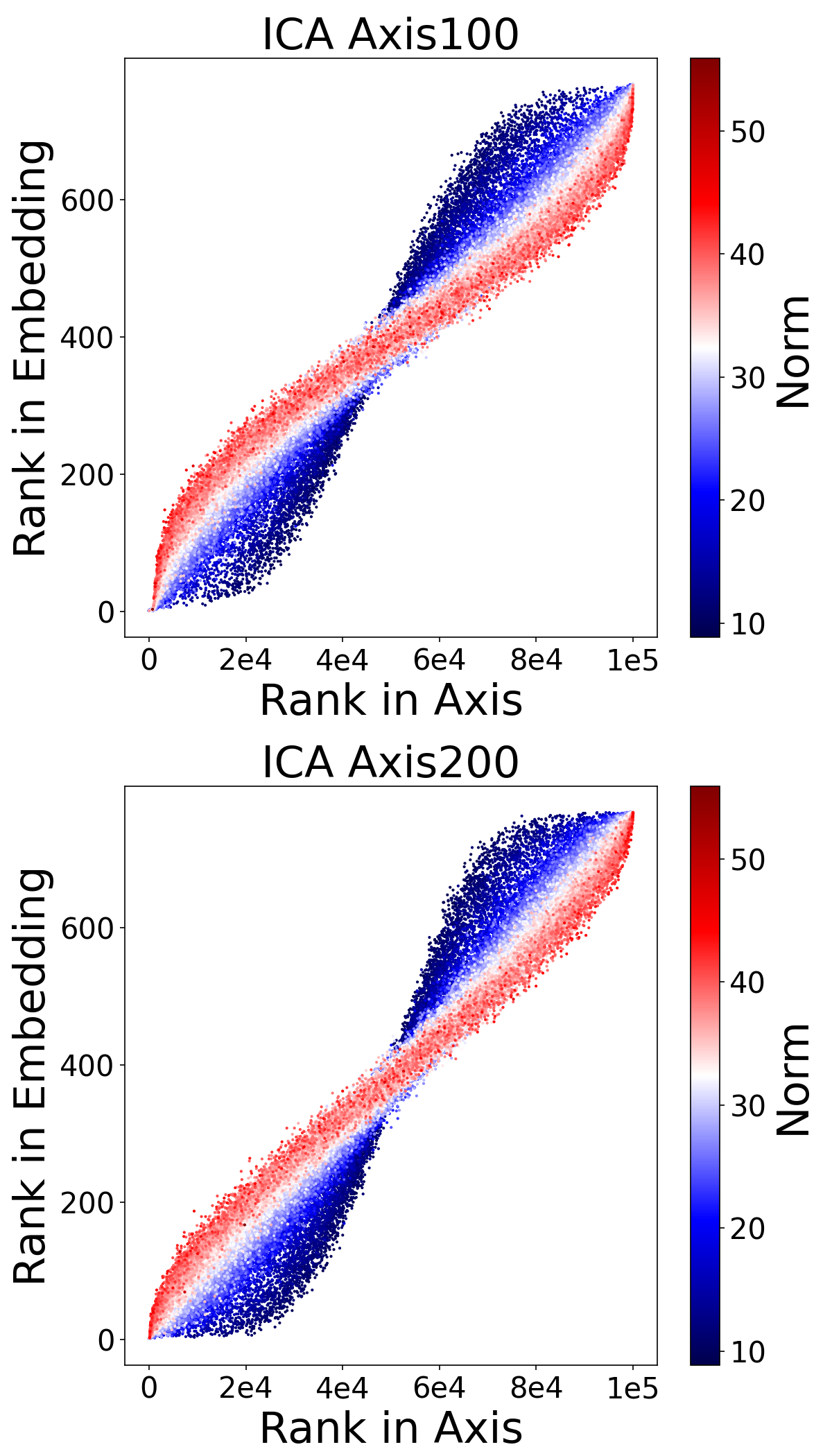
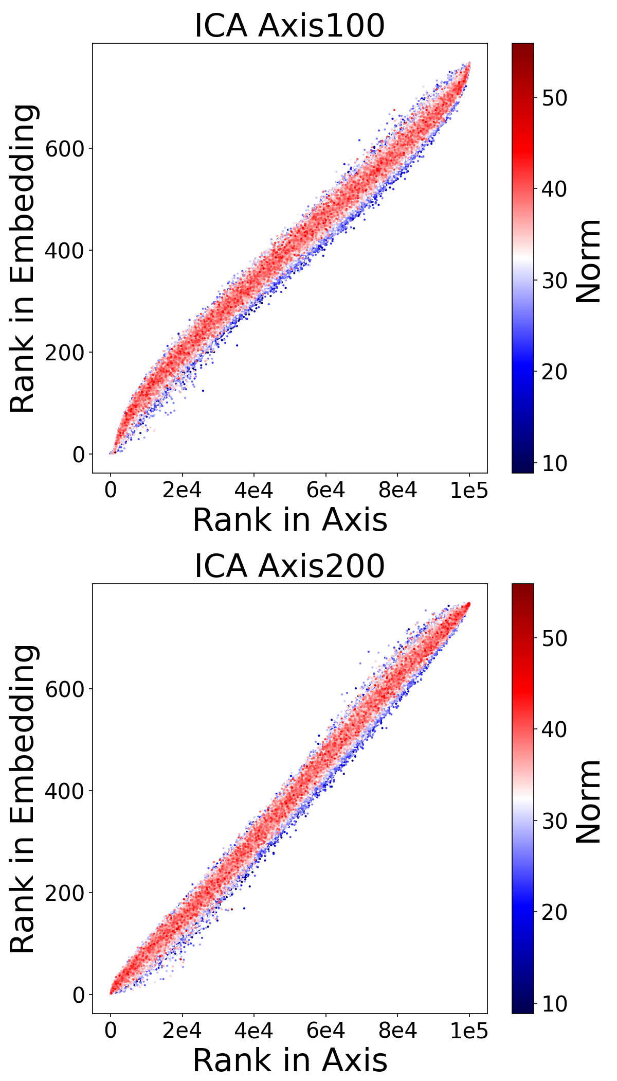
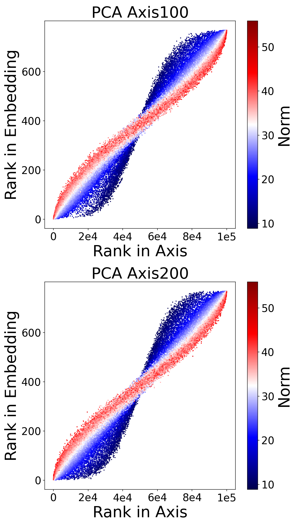
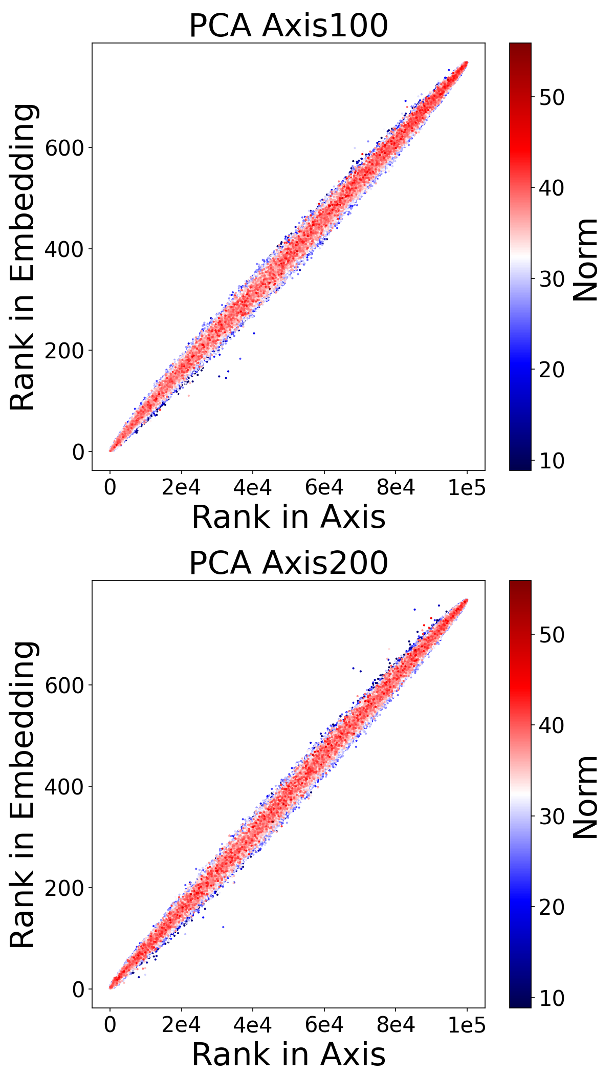
In Section 4, for the $150$th axis of the ICA-transformed embeddings, Fig. 3 shows the ranks within the axis and within each embedding before and after normalization. This section extends similar experiments to other axes and to the PA-transformed embeddings.

For the $100$th and $200$th axes of the ICA-transformed embeddings, Fig. 12 shows the ranks within the axis and within each embedding before and after normalization. Similar to Fig. 3, norm-derived artifacts are present before normalization and disappear after normalization.

Experiments were also performed on the PCA-transformed embeddings, and Fig. 13 shows the results. Since the norm represents the importance of the word and the direction represents the meaning of the word Yokoi et al. (2020); Oyama et al. (2023), the results are similar to those of the ICA-transformed embeddings.

(a) Before Normalization

(b) After Normalization

Figure 12: Scatterplots for the $100$th and $200$th axes of the ICA-transformed GloVe embeddings, (a) before and (b) after normalization, showing ranks within the axis and within each embedding, colored by the norms of the embeddings.

(a) Before Normalization

(b) After Normalization

Figure 13: Scatterplots for the $100$th and $200$th axes of the PCA-transformed GloVe embeddings, (a) before and (b) after normalization, showing ranks within the axis and within each embedding, colored by the norms of the embeddings.

(a) Before Normalization

(b) After Normalization

Figure 14: Scatterplots for the $100$th and $200$th axes of the ICA-transformed BERT embeddings, (a) before and (b) after normalization, showing ranks within the axis and within each embedding, colored by the norms of the embeddings.

(a) Before Normalization

(b) After Normalization

Figure 15: Scatterplots for the $100$th and $200$th axes of the PCA-transformed BERT embeddings, (a) before and (b) after normalization, showing ranks within the axis and within each embedding, colored by the norms of the embeddings.

A.2 BERT

Experiments similar to those described in Appendix A.1 and Section 5 are performed using the BERT embeddings. Similar to Fig. 6, we used the embeddings published by Yamagiwa et al. (2023) as the ICA-transformed and PCA-transformed BERT embeddings.

A.2.1 Rank comparison of component values

Using the BERT embeddings, for the $100$th and $200$th axes of the ICA-transformed and PCA-transformed embeddings, Figs. 14 and 15 show the ranks within the axis and within each embedding before and after normalization. Even for the dynamic BERT embeddings, the results are similar to the static GloVe embeddings in Figs. 12 and 13.

	Axis	Top1	Top2	Top3	Top4	Top5	Top6	Top7	Top8	Top9	Top10	Meaning
Normalized ICA	53	salts	solvents	chlorine	hydrogen	inorganic	ammonia	chloride	flammable	sulfide	sulfur	[chemistry]
	68	proteins	protein	genes	gene	mrna	receptor	transcription	activation	p53	rna	[biology]
	141	spacecraft	astronauts	orbit	nasa	astronaut	orbiter	space	orbiting	mars	atlantis	[space]
	194	light	ultraviolet	infrared	sunlight	uv	shadows	bright	illumination	glow	illuminate	[spectrum]
	197	virus	h5n1	influenza	flu	contagious	outbreak	swine	avian	viruses	pandemic	[virology]
Normalized PCA	80	zhongshan	solar	optical	shyh	electrics	wafers	nerpa	selden	wbut	reutemann	[PC80]
	92	woodcuts	natrun	eriboll	linocuts	shamva	cellblock	hafslund	g2	heidelberg	venter	[PC92]
	152	sidebar	maternal	smoker	customizer	non-qualified	sufia	foundresses	frosting	traudl	romm	[PC152]
	153	monogamous	lifespan	necessitate	loyals	supplementation	skrall	zng	gietzen	remnant	well-meaning	[PC153]
	222	replication	isley	guaporé	bobos	pawhuska	foss	rigoberto	angara	laporta	200-250	[PC222]

Table 2: For the normalized ICA-transformed and PCA-transformed embeddings of ultraviolet in Fig. 2, the axes of the top 5 component values are focused on, and their top 10 words are shown. For ICA, the meanings of the axes are interpreted from these listed words and labeled such as [chemistry]. For PCA, however, since it is difficult to interpret the meanings of the axes, they are simply labeled such as [PC80].

Figure 16: For 10,000 randomly sampled pairs of ICA-transformed embeddings $S,S^{\prime}\in\mathbb{R}^{d}$, the histogram of the cosine similarity $\cos(S,S^{\prime})$ is displayed. Since cosine similarities are invariant under the orthogonal transformation, exactly the same plot is also obtained from PCA-transformed embeddings. The theoretical probability density of (12) is almost identical to the observed histogram. The theory in Appendix C is also supported by the inverse of the variance, ${309.663}\approx d$ for $d=300$. The observed cosine similarities in Fig. 5 are also indicated as vertical lines.

(a) Components

(b) Component-wise products

(c) Component-wise products (magnified)

Figure 17: For 10,000 randomly sampled pairs of normalized ICA-transformed embeddings $\hat{S},\hat{S}^{\prime}\in\mathbb{R}^{d}$, (a) the histogram of the components $\hat{S}_{i}$ and (b, c) the histograms of the products of the components $\hat{S}_{i}\hat{S}_{i}^{\prime}$ are displayed. The theoretical probability density of (14) for the components and that of (15) for the component-wise products are almost identical to their observed histograms. The theory in Appendix C is also supported by the inverse of the variance, ${300.005}\approx d$ in (a) and $89{,}917.992\approx d^{2}$ in (b, c) for $d=300$. The observed component values in Fig. 2 are also indicated as vertical lines.

(a) Components

(b) Component-wise products

(c) Component-wise products (magnified)

Figure 18: The plots for the normalized PCA-transformed embeddings are displayed in the same manner as in Fig. 17. The inverse of the variance is $300.000\approx d$ in (a) and $90{,}108.283\approx d^{2}$ in (b, c) for $d=300$.

Axis	Top1	Top2	Top3	Top4	Top5	Top6	Top7	Top8	Top9	Top10	Meaning
61	naval_2	sea_1	marine_2	vessels_2	sea_2	sea_6	vessel_0	naval_1	ships_1	ship_2	[sea]
207	australian_1	australian_2	new_1	wales_0	australia_0	sydney_1	south_0	queensland_0	sydney_0	australia_3	[australia]
250	neighborhood_3	street_12	drag_0	of_209	central_7	district_12	street_29	street_8	heart_5	in_680	[district]
303	curb_2	prevent_0	avoid_0	reduce_12	reducing_1	##d_39	reduce_3	control_2	prevent_7	prevent_10	[control]
338	makes_2	allowed_7	forcing_1	bring_11	triggered_1	lead_2	illustrated_0	make_65	triggered_2	force_8	[causative verbs]
344	the_1179	the_1976	of_1927	were_41	were_89	the_1593	also_64	the_1180	been_154	been_81	[numbers]
354	agency_17	agency_1	strategy_2	company_59	country_7	group_41	law_7	charity_1	company_13	pact_0	[orgnization]
521	bail_2	bail_8	pay_23	walk_0	##avi_1	roll_0	walk_5	cop_1	go_28	turn_5	[action]
558	ground_10	side_2	front_10	side_18	corner_2	scene_3	sides_6	trail_0	hand_8	hand_19	[location]
572	more_167	a_244	##some_0	with_434	and_1493	good_38	and_246	with_318	more_148	the_2200	[linking words]

Table 3: For the normalized ICA-transformed embeddings of shore_0, shore_1, and shore_2 in Fig. 6, the axes of the top 4 component values for each embedding are focused. The number of axes is 10, excluding duplicates, and the top 10 words of the axes are shown.

shore_0	Last month , the two companies sliced their dividends and sold billions of dollars of special stock to raise capital and shore up their finances .
shore_1	Working for a Sydney newspaper , my daughter covered a dreadful 1994 fire where , on one of the suburban streets of Sydney ’s North Shore ,
	the fire jumped the road and , for some terrifying seconds , took all the oxygen with it .
shore_2	Coastguards from Clevedon and Weston searched the shore while two lifeboats and two helicopters were also involved .

Table 4: Sentences for shore_0, shore_1, and shore_2 in Fig. 6. Note that shore_0 is a verb, while shore_1 and shore_2 are nouns.

A.2.2 Comparison of ICA and PCA

The experiments in Section 5 were also performed on the BERT embeddings. Fig. 11 shows a plot of the component values for each axis, sorted in descending order and averaged. Fig. 11 shows a plot of the component values for each embedding, sorted in descending order and averaged. The dynamic BERT embeddings also show similar results to the static GloVe embeddings shown in Fig. 4.

Appendix B Details of examples that illustrate our interpretation of cosine similarity

For the normalized ICA-transformed and PCA-transformed embeddings of ultraviolet in Fig. 2, Table 2 shows the top 10 words for the axes of the top 5 component values. The semantic interpretations of the axes are also provided for ICA-transformed embeddings, but such interpretations are challenging for PCA-transformed embeddings.

Based on Table 2, Fig. 5 illustrates our interpretation of cosine similarity using the top word of each axis: salts, proteins, spacecraft, light, and virus. The cosine similarities are decomposed into component-wise similarities, thus providing semantic interpretations of the similarities.

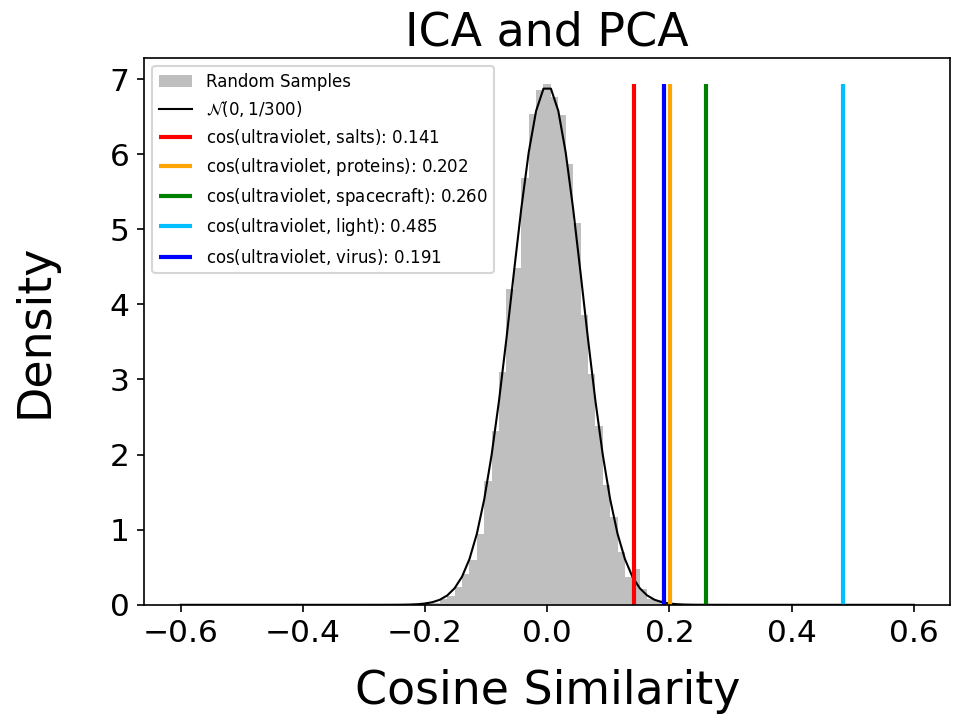
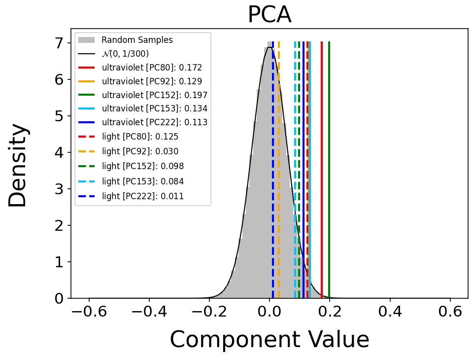
The observed and theoretical distributions of the cosine similarities are exhibited in Fig. 16. The histogram and the theoretical curve of the probability density function clearly suggest that the distribution theory in Appendix C.1 is strongly supported and that the cosine similarities are normally distributed with mean zero and variance $1/d$. However, when embeddings are centered but not whitened, which violates the assumption in Appendix C.1, the variance should tend to be larger than $1/d$. In such a case, the inverse of the variance would provide an effective dimensionality of the embeddings.

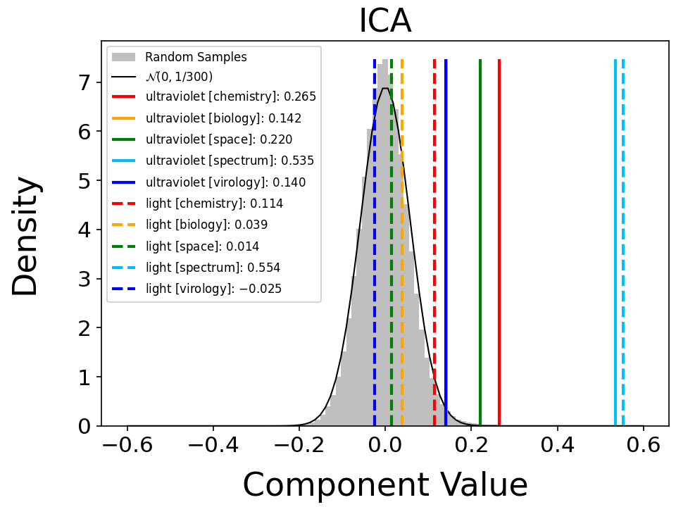
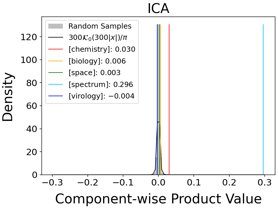
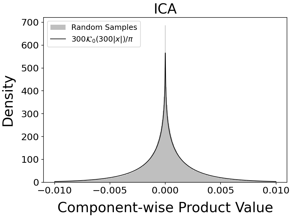
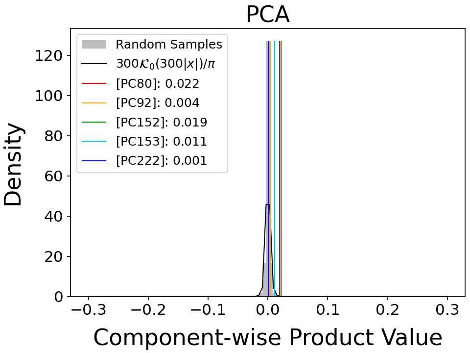
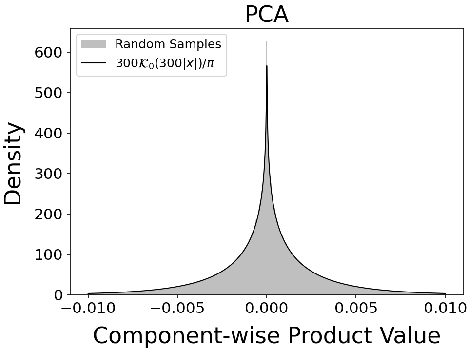
The observed and theoretical distributions of the components and the component-wise products are exhibited in Figs. 17 and 18. The histograms and the theoretical curves of the probability density functions clearly suggest that the distribution theory in Appendices C.2 and C.3 is strongly supported. The components are normally distributed with mean zero and variance $1/d$, and the probability density function of the component-wise products is expressed by the modified Bessel function, where the mean is zero and the variance is $1/d^{2}$. Interestingly, while the theory was originally provided for ICA-transformed embeddings, the experiments suggest that the theory also applies to the PCA-transformed embeddings.

In Figs. 16, 17, and 18, the observed values, indicated as vertical lines, are compared to their respective distributions to identify the significance of the values. By multiplying the values by the inverse of the standard deviations, these values can be easily interpreted. Thus, $\sqrt{d}\cos(S,S^{\prime})$, $\sqrt{d}\hat{S}_{i}$, and $d\hat{S}_{i}\hat{S}_{i}^{\prime}$ may be used for numerical comparisons.

Appendix C Distribution of cosine similarity, component values and their products

C.1 Cosine similarity

Let us consider two random vectors $X=(X_{1},\ldots,X_{d}),Y=(Y_{1},\ldots,Y_{d})\in\mathbb{R}^{d}$ with elements of mean zero $\mathbb{E}(X_{\ell})=\mathbb{E}(Y_{\ell})=0$ and variance one $\mathbb{E}(X_{\ell}^{2})=\mathbb{E}(Y_{\ell}^{2})=1$. We assume that the elements $X_{1},\ldots,X_{d}$ and $Y_{1},\ldots,Y_{d}$ are independent. Then, for sufficiently large $d$, the cosine similarity $\cos(X,Y)$ asymptotically follows $\mathcal{N}(0,1/d)$, the normal distribution with mean 0 and variance $1/d$,

$$\cos(X,Y)\sim\mathcal{N}(0,1/d).$$ (12)

This is easily shown as follows; a more general argument can be found in Appendix C of Yamagiwa et al. (2024). First note that $\mathbb{E}(X_{\ell}Y_{\ell})=\mathbb{E}(X_{\ell})\mathbb{E}(Y_{\ell})=0$, $\mathbb{E}(X_{\ell}^{2}Y_{\ell}^{2})=\mathbb{E}(X_{\ell}^{2})\mathbb{E}(Y_{\ell}^{2})=1$. Thus the inner product, if scaled by dimension, $d^{-1/2}\langle X,Y\rangle=d^{-1/2}\sum_{\ell=1}^{d}X_{\ell}Y_{\ell}$ has mean zero and variance one. Thus, according to the central limit theorem,

$$d^{-1/2}\langle X,Y\rangle\sim\mathcal{N}(0,1)$$ (13)

for sufficiently large $d$. It also follows from the law of large numbers that $d^{-1}\|X\|^{2}=d^{-1}\sum_{\ell=1}^{d}X_{\ell}^{2}$ converges in probability to $\mathbb{E}(X_{\ell}^{2})=1$, and similarly $d^{-1}\|Y\|^{2}\to 1$ in probability. Therefore,

$$\sqrt{d}\cos(X,Y)=\frac{d^{-1/2}\langle X,Y\rangle}{\sqrt{d^{-1}\|X\|^{2}}\sqrt{d^{-1}\|Y\|^{2}}}$$

converges to (13), thereby concluding (12).

C.2 Component values

Let $S=(S_{1},\ldots,S_{d})\in\mathbb{R}^{d}$ be a random vector representing ICA-transformed embeddings, and let $e_{i}=(0,\ldots,0,1,0,\ldots,0)\in\mathbb{R}^{d}$ be the one-hot vector with a one at the $i$-th element. Then, $\hat{S}_{i}=\cos(S,e_{i})$ represents the $i$-th component of the normalized ICA-transformed embeddings. Although $e_{i}$ is not a random vector, formally letting $X=S$ and $Y=e_{i}$ in (12) gives

$$\hat{S}_{i}\sim\mathcal{N}(0,1/d)$$ (14)

for sufficiently large $d$. Considering $S$ and $e_{i}$ in the original coordinate system before the ICA-transformation, they can be regarded as almost random, which suggests that the formal argument above is valid.

C.3 Product of two component values

Let $\hat{S}=(\hat{S}_{1},\ldots,\hat{S}_{d}),\hat{S}^{\prime}=(\hat{S}_{1}^{\prime},\ldots,\hat{S}_{d}^{\prime})\in\mathbb{R}^{d}$ be two independent random vectors representing normalized ICA-transformed embeddings. We consider $Z_{i}=\hat{S}_{i}\hat{S}_{i}^{\prime}$, the $i$-th element of the component-wise product of $\hat{S}$ and $\hat{S}^{\prime}$. Then, for sufficiently large $d$, the probability density function of $Z_{i}$ is

$$Z_{i}\sim(d/\pi)K_{0}(d|Z_{i}|),$$ (15)

where $K_{0}(\cdot)$ is the modified Bessel function of the second kind of order zero. This result follows directly from Theorem 2.1 of Nadarajah and Pogány (2016), assuming that $\hat{S}_{i}$ and $\hat{S}_{i}^{\prime}$ are independently distributed as $\mathcal{N}(0,1/d)$. The mean of $Z_{i}$ is $\mathbb{E}(Z_{i})=\mathbb{E}(\hat{S}_{i}\hat{S}_{i}^{\prime})=\mathbb{E}(\hat{S}_{i})\mathbb{E}(\hat{S}_{i}^{\prime})=0$ and the variance of $Z_{i}$ is $\mathbb{E}(Z_{i}^{2})=\mathbb{E}(\hat{S}_{i}^{2}\hat{S}_{i}^{\prime 2})=\mathbb{E}(\hat{S}_{i}^{2})\mathbb{E}(\hat{S}_{i}^{\prime 2})=1/d^{2}$.

Appendix D Details of examples of ICA-transformed BERT embeddings

In Section 7.1, Fig. 6 showed the semantic components of the normalized ICA-transformed embeddings of shore_0, shore_1, and shore_2 using the embeddings published by Yamagiwa et al. (2023). For each shore, the axes of the top 4 component values, excluding duplicates, were selected, and the top 10 words of these $10$ axes are shown in Table 3. Similar to the ICA-transformed GloVe embeddings, the axes of the ICA-transformed BERT embeddings are also interpretable. Additionally, the sentences containing these tokens are shown in Table 4. While shore_0 is a verb, both shore_1 and shore_2 are nouns. Comparing the nouns shore_1 and shore_2, we find that since shore_1 is specifically part of Sydney’s North Shore, the normalized ICA-transformed embedding of shore_1 in Fig. 6 has a large semantic component of [australia]. This result also shows that the BERT embeddings are well contextualized.

Appendix E Examples of ICA-transformed embeddings in multiple languages

	Axis	Top1	Top2	Top3	Top4	Top5	Top6	Top7	Top8	Top9	Top10	Meaning
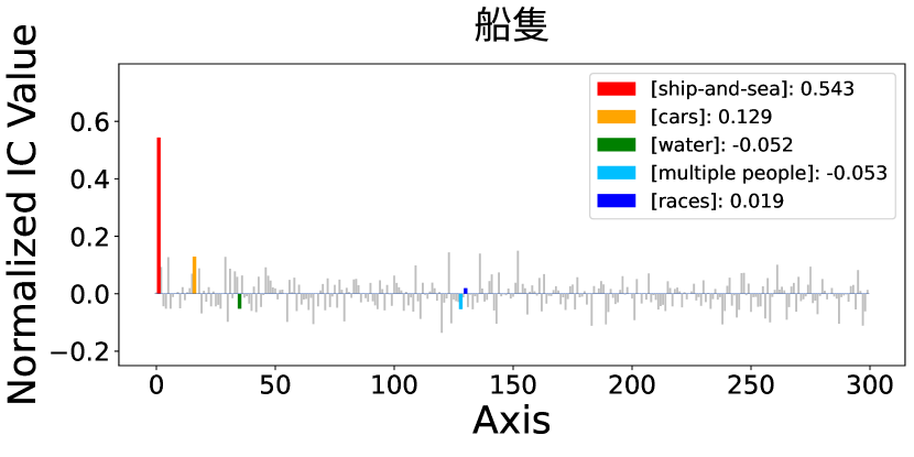
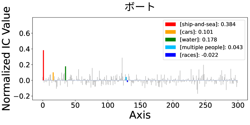
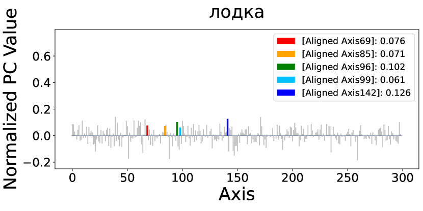
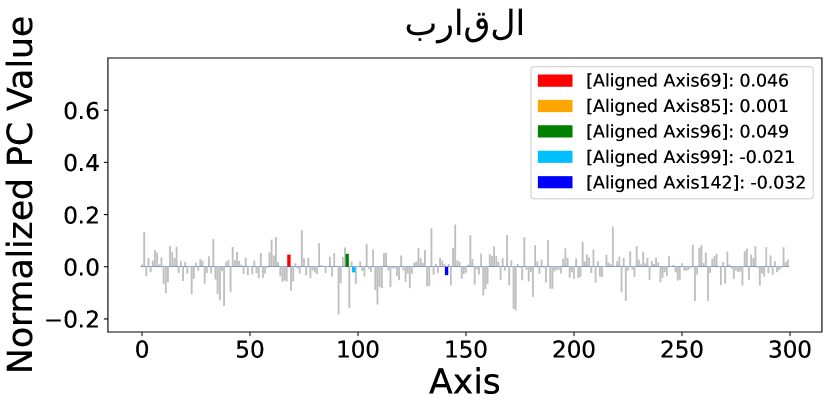
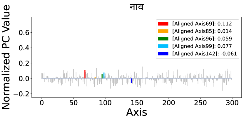
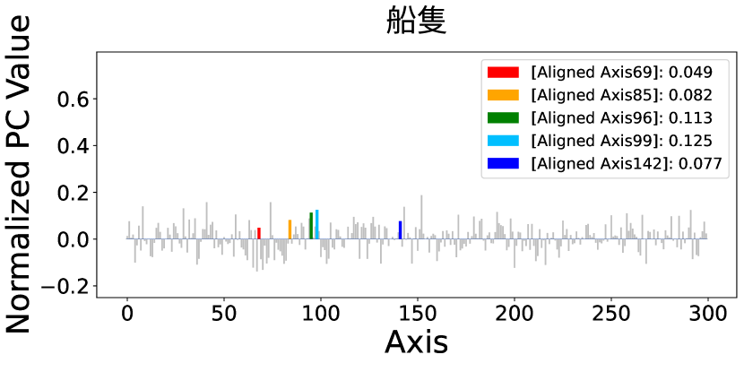
Normalized ICA	2	boat	sailing	sail	ship	boats	sea	ships	海	open-sea	ocean	[ship-and-sea]
	17	car.	car	bmw	4-door	car–	v-6	2-dr	u.s.-market	car–and	2-door	[cars]
	36	water	rivers	reservoir	water–the	river-water	water.	water–	black-water	basin	de-water	[water]
	129	12-man	five-man	five-person	six-member	seven-man	14-member	12-person	seven-person	12-member	three-person	[multiple people]
	131	race	races	racing	race.	racer	race.-	.race	rider	laps	race-like	[races]
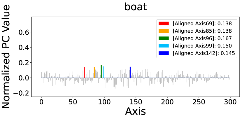
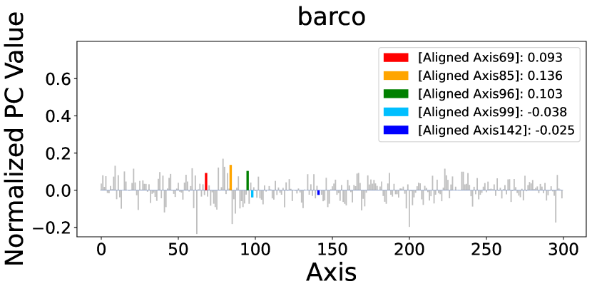
Normalized PCA	69	bit-field	torn	out-of-round	unused	final-	3-space	bad.2.	cup	too-large	.language	[Aligned Axis69]
	85	2-the	name-called	accusations	t-head	down.1.	1-the	relata	attacked	flew	two-place	[Aligned Axis85]
	96	government-run	trading	state-run	military-run	kids-only	trade	floating	e-a	sirven	trade.	[Aligned Axis96]
	99	white-red-white	-green	white-blue	red-green	white-red	.hair	color	’k	voz	poles	[Aligned Axis99]
	142	business-process	source-to-pay	time-to-market	menudo	s-u	5-6-11	pulse	cost	news-	time-to-value	[Aligned Axis142]

Table 5: For the normalized ICA and PCA transformed embeddings of boat in Figs 19 and 20, the axes of the top 5 component values are focused and their top 10 words are shown. For PCA, since it is difficult to interpret the meanings of the axes, they are simply labeled such as [Aligned Axis69]. Similar to GloVe, the meanings of the axes of the ICA-transformed fastText embeddings are interpretable.

(a) English

(b) Spanish

(c) Russian

(d) Arabic

(e) Hindi

(f) Chinese

(g) Japanese

Figure 19: For boat and its translations, the normalized ICA-transformed embeddings are shown as bar graphs. These axes are aligned by the correlation coefficients between English and the other languages. The axes of the top 5 component values in English are highlighted with their meanings. The component values of these axes are shown in each language. See Table 5 for the top 10 words of these axes.

(a) English

(b) Spanish

(c) Russian

(d) Arabic

(e) Hindi

(f) Chinese

(g) Japanese

Figure 20: For boat and its translations, the normalized PCA-transformed embeddings are shown as bar graphs. These axes are aligned by the correlation coefficients between English and the other languages. The axes of the top 5 component values in English are highlighted with their meanings. The component values of these axes are shown in each language. See Table 5 for the top 10 words of these axes.

Figure 21: Bar graphs of the normalized ICA-transformed embeddings of woman, girl, and man, showing each component value of [female].

$p=1$ $p=5$ $p=10$ $p=50$ $p=100$ $p=300$ Tasks PCA ICA PCA ICA PCA ICA PCA ICA PCA ICA PCA ICA Similarity MEN 0.11 0.45 0.31 0.59 0.45 0.63 0.69 0.72 0.73 0.74 0.75 0.75 WS353 -0.02 0.19 0.12 0.45 0.25 0.49 0.49 0.55 0.54 0.56 0.57 0.57 WS353R 0.04 0.16 0.15 0.44 0.22 0.46 0.43 0.49 0.48 0.49 0.51 0.51 WS353S 0.01 0.31 0.17 0.56 0.34 0.60 0.62 0.67 0.66 0.70 0.69 0.69 SimLex999 0.00 0.10 0.11 0.21 0.19 0.25 0.35 0.35 0.38 0.37 0.40 0.40 RW 0.08 0.13 0.15 0.20 0.18 0.22 0.27 0.30 0.30 0.32 0.34 0.34 RG65 0.42 0.42 0.53 0.57 0.61 0.64 0.71 0.76 0.74 0.79 0.78 0.78 MTurk 0.22 0.42 0.36 0.58 0.49 0.61 0.64 0.65 0.66 0.66 0.64 0.64 Average 0.11 0.27 0.24 0.45 0.34 0.49 0.53 0.56 0.56 0.58 0.59 0.59 Analogy capital-common-countries 0.00 0.22 0.01 0.51 0.24 0.62 0.93 0.94 0.95 0.94 0.95 0.95 capital-world 0.01 0.05 0.04 0.15 0.21 0.29 0.91 0.90 0.95 0.93 0.95 0.95 city-in-state 0.00 0.00 0.00 0.13 0.05 0.21 0.49 0.55 0.59 0.60 0.67 0.67 currency 0.00 0.00 0.00 0.00 0.00 0.03 0.06 0.11 0.11 0.12 0.12 0.12 family 0.00 0.00 0.01 0.24 0.14 0.36 0.74 0.74 0.84 0.84 0.88 0.88 gram1-adjective-to-adverb 0.00 0.00 0.00 0.00 0.02 0.02 0.16 0.16 0.19 0.20 0.21 0.21 gram2-opposite 0.00 0.00 0.00 0.00 0.02 0.02 0.18 0.18 0.24 0.23 0.26 0.26 gram3-comparative 0.00 0.00 0.02 0.19 0.17 0.42 0.79 0.82 0.84 0.86 0.88 0.88 gram4-superlative 0.00 0.00 0.04 0.15 0.14 0.28 0.57 0.63 0.66 0.69 0.69 0.69 gram5-present-participle 0.00 0.00 0.01 0.15 0.07 0.36 0.64 0.68 0.69 0.70 0.69 0.69 gram6-nationality-adjective 0.01 0.22 0.14 0.37 0.52 0.49 0.91 0.92 0.92 0.92 0.93 0.93 gram7-past-tense 0.00 0.00 0.03 0.09 0.09 0.21 0.50 0.52 0.56 0.57 0.60 0.60 gram8-plural 0.00 0.00 0.01 0.15 0.13 0.27 0.70 0.69 0.75 0.74 0.76 0.76 gram9-plural-verbs 0.00 0.00 0.02 0.20 0.12 0.37 0.48 0.57 0.57 0.60 0.58 0.58 jj_jjr 0.00 0.00 0.03 0.13 0.14 0.29 0.53 0.56 0.60 0.63 0.66 0.66 jj_jjs 0.00 0.00 0.03 0.11 0.10 0.22 0.41 0.49 0.49 0.54 0.51 0.51 jjr_jj 0.00 0.00 0.01 0.03 0.05 0.10 0.45 0.46 0.53 0.54 0.54 0.54 jjr_jjs 0.00 0.00 0.03 0.08 0.09 0.20 0.38 0.49 0.49 0.56 0.55 0.55 jjs_jj 0.00 0.00 0.02 0.05 0.05 0.10 0.36 0.36 0.43 0.44 0.48 0.48 jjs_jjr 0.00 0.01 0.01 0.14 0.09 0.29 0.55 0.59 0.60 0.63 0.63 0.63 nn_nnpos 0.00 0.02 0.00 0.13 0.06 0.22 0.35 0.35 0.39 0.39 0.42 0.42 nn_nns 0.00 0.03 0.00 0.24 0.10 0.39 0.62 0.63 0.69 0.68 0.74 0.74 nnpos_nn 0.00 0.06 0.00 0.21 0.05 0.29 0.41 0.41 0.43 0.42 0.45 0.45 nns_nn 0.00 0.06 0.01 0.24 0.11 0.36 0.56 0.55 0.61 0.59 0.64 0.64 vb_vbd 0.00 0.01 0.03 0.10 0.13 0.23 0.55 0.53 0.56 0.54 0.58 0.58 vb_vbz 0.00 0.00 0.02 0.16 0.11 0.34 0.66 0.72 0.74 0.76 0.76 0.76 vbd_vb 0.00 0.01 0.02 0.09 0.08 0.27 0.60 0.64 0.66 0.67 0.69 0.69 vbd_vbz 0.00 0.00 0.03 0.11 0.10 0.29 0.56 0.60 0.63 0.63 0.63 0.63 vbz_vb 0.00 0.00 0.02 0.09 0.15 0.27 0.77 0.75 0.80 0.79 0.82 0.82 vbz_vbd 0.01 0.00 0.04 0.05 0.14 0.14 0.57 0.51 0.59 0.56 0.55 0.55 Average 0.00 0.02 0.02 0.14 0.12 0.26 0.55 0.57 0.60 0.61 0.63 0.63

Table 6: The performance of ICA-transformed and PCA-transformed embeddings when reducing the number of non-zero normalized component-wise products to $p$ and then computing cosine similarity. The values in the table correspond to Top 1 accuracy for analogy tasks and Spearman’s rank correlation for word similarity tasks.

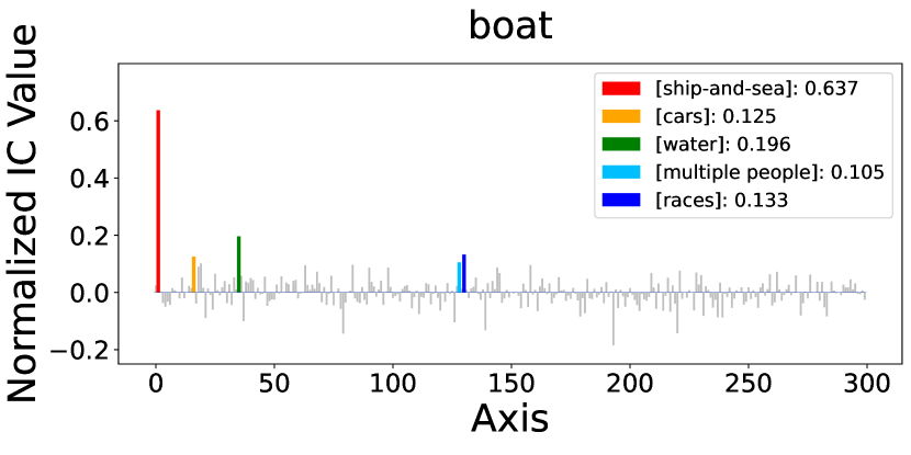
Yamagiwa et al. (2023) showed that common semantic axes exist between ICA-transformed embeddings of different languages, and matched these axes by their correlations. They used the fastText Bojanowski et al. (2017) embeddings for their experiments, and their ICA-transformed and PCA-transformed embeddings are published.

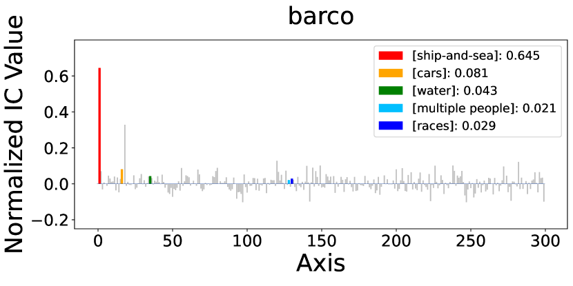
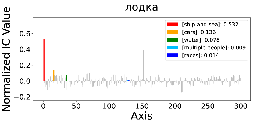
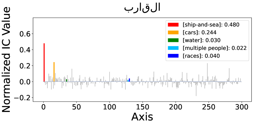
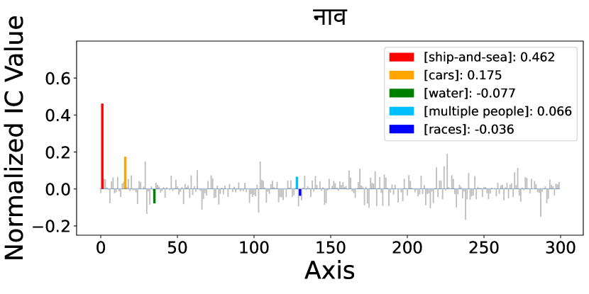
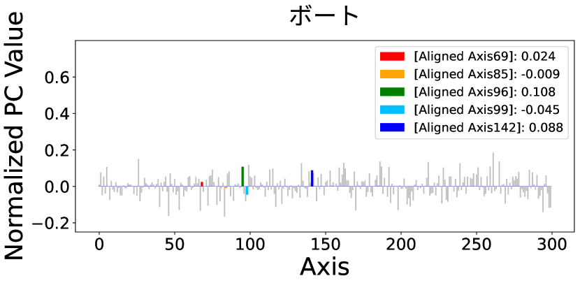
As an example, we analyzed the embedding of boat and compared it with those of its translations in Spanish, Russian, Arabic, Hindi, Chinese, and Japanese. Figs. 19 and 20 show the bar graphs of the normalized ICA-transformed and PCA-transformed embeddings, respectively, for these languages. Table 5 shows the top 10 words of the axes of the top 5 component values in each embedding of boat. These results show that while the semantic component of [ship-and-sea] is the largest for all normalized ICA-transformed embeddings in Fig. 19, there is no such semantic component for the normalized PCA-transformed embeddings in Fig. 20.

Appendix F Details of examples for the ablation of the semantic component of [female]

In section, Fig. 9 showed scatterplots of normalized ICA-transformed embeddings for woman and girl, and woman and girl. Fig. 21 shows bar graphs of these embeddings. The graphs for woman and girl are similar in shape. On the other hand, the graphs for woman and man show differences in the semantic component of [female], although other parts are broadly similar.

Appendix G Details of the downstream tasks used to examine the sparsity in Section 7.2

We performed analogy and word similarity tasks following the settings of Yamagiwa et al. (2024). We explain the details of the tasks using the ICA-transformed embeddings, and apply the same procedure to the PCA-transformed embeddings. We define $\llbracket d\rrbracket:=\{1,\ldots,d\}$ and let $p\,(\leq d)$ be the number of non-zero product components.

G.1 Word similarity tasks

(a) $p=1$

(b) $p=10$

(c) $p=100$

Figure 22: Comparison of the scatterplots for the sum of the top $p$ component-wise products and the cosine similarity for the normalized ICA-transformed and PCA-transformed embeddings at (a) $p=1$, (b) $10$, and (c) $100$. We used word pairs from the word similarity tasks. For $p=1$, $10$, and $100$, the correlation coefficients for ICA were $0.619$, $0.876$, and $0.979$, respectively, while for PCA they were $0.432$, $0.761$, and $0.982$. See Fig. 23 for the correlation coefficients for other values of $p$.

Figure 23: Comparison of correlation coefficients between the sum of the top $p$ component-wise products and the cosine similarity for normalized ICA-transformed and PCA-transformed embeddings. We used word pairs from the word similarity tasks.

G.1.1 Setting

We used several datasets, including MEN Bruni et al. (2014), MTurk Radinsky et al. (2011), RG65 Rubenstein and Goodenough (1965), RW Luong et al. (2013), SimLex999 Hill et al. (2015), WS353 Finkelstein et al. (2002), WS353R (WS353 Relatedness), and WS353S (WS353 Similarity). In these tasks, we compute the cosine similarity $\cos{(w_{i},w_{j})}$ between words $w_{i}$ and $w_{j}$ and compare it with human-rated similarity scores. Spearman’s rank correlation is used as the evaluation metric.

G.1.2 Details of $p$ non-zero products

We explain the top $p$ component-wise products used for the similarity tasks.

As seen in (6), since the cosine similarity between words $w_{i}$ and $w_{j}$ is expressed as the sum of the component-wise products, we consider the index set of the top $p$ component-wise products:

$$\text{Top}_{p}:=\mathop{\operatorname{argmax}}_{\ell\in\llbracket d\rrbracket}{}_{p}\,\hat{s}_{i}^{(\ell)}\,\hat{s}_{j}^{(\ell)}.$$ (16)

If $p=d$, then $\text{Top}_{p}=\llbracket d\rrbracket$.

Then, based on the cosine similarity expression in (6), we express the top $p$ component-wise products as

$$\sum_{\ell\in\text{Top}_{p}}\hat{s}_{i}^{(\ell)}\,\hat{s}_{j}^{(\ell)}.$$ (17)

G.2 Analogy tasks

G.2.1 Setting

We used the Google Analogy Test Set Mikolov et al. (2013a), which consists of 14 types of analogy tasks, and the Microsoft Research Syntactic Analogies Dataset Mikolov et al. (2013d), which consists of 16 types. In these tasks, if $w_{1}$ corresponds to $w_{2}$, then we predict $w_{4}$ to which $w_{3}$ corresponds. To do this, the vector $s_{2}-s_{1}+s_{3}$ is computed, and if the index of the closest word embedding to the vector in terms of cosine similarity,

$$\mathop{\operatorname{argmax}}_{i\in\llbracket n\rrbracket}{}\,\cos{(\mathbf{s}_{i_{2}}-\mathbf{s}_{i_{1}}+\mathbf{s}_{i_{3}},\mathbf{s}_{i})},$$ (18)

is $i_{4}$, then it is considered correct (top 1 accuracy).

G.2.2 Details of $p$ non-zero products

We explain the top $p$ component-wise products used for the analogy tasks.

Based on Appendix G.2.1, we define $\mathbf{s}_{i_{1},i_{2},i_{3}}:=\mathbf{s}_{i_{2}}-\mathbf{s}_{i_{1}}+\mathbf{s}_{i_{3}}$ and normalize it as

$$\hat{\mathbf{s}}_{i_{1},i_{2},i_{3}}:=\frac{\mathbf{s}_{i_{1},i_{2},i_{3}}}{\|\mathbf{s}_{i_{1},i_{2},i_{3}}\|}=\left(\hat{s}_{i_{1},i_{2},i_{3}}^{(\ell)}\right)_{\ell=1}^{d}\in\mathbb{R}^{d}.$$ (19)

Then, following the cosine similarity expression in (6), (18) can be rewritten as

$$\mathop{\operatorname{argmax}}_{i\in\llbracket n\rrbracket}{}\,\sum_{\ell=1}^{d}\hat{s}_{i_{1},i_{2},i_{3}}^{(\ell)}\,\hat{s}_{i}^{(\ell)}.$$ (20)

Based on (20), we consider the index set of top $p$ component-wise products for each word $w_{i}$:

$$\text{Top}_{p}^{i}:=\mathop{\operatorname{argmax}}_{\ell\in\llbracket d\rrbracket}{}_{p}\,\hat{s}_{i_{1},i_{2},i_{3}}^{(\ell)}\,\hat{s}_{i}^{(\ell)}$$ (21)

If $p=d$, then $\text{Top}_{p}^{i}=\llbracket d\rrbracket$.

Then, following the expression in (20), we use the top $p$ component-wise products and predict the index of the answer word as follows:

$$\mathop{\operatorname{argmax}}_{i\in\llbracket n\rrbracket}{}\,\sum_{\ell\in\text{Top}_{p}^{i}}\hat{s}_{i_{1},i_{2},i_{3}}^{(\ell)}\,\hat{s}_{i}^{(\ell)}.$$ (22)

G.3 Results

Table 6 shows the results for the tasks with $p=1$, $5$, $10$, $50$, $100$, and $300$. The performance of the ICA-transformed embeddings is better than that of the PCA-transformed embeddings. As seen in Fig. 7, the difference in performance between ICA and PCA is larger for the word similarity tasks than for the analogy tasks. This is probably because in the word similarity tasks, the semantic components are used directly, as shown in (17). On the other hand, in the analogy tasks, the component values of the normalized vector $\hat{\mathbf{s}}_{i_{1},i_{2},i_{3}}$ are used, as shown in (22).

G.4 Relation between the sum of the top $p$ products and cosine similarity

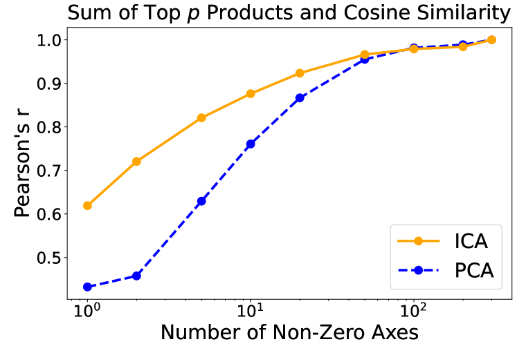
As seen in Appendix G.1, in the word similarity tasks, we compared performance using the sum of the top $p$ component-wise products for the normalized ICA-transformed and PCA-transformed embeddings. In this section, we examine the relation between this sum and the original cosine similarity.

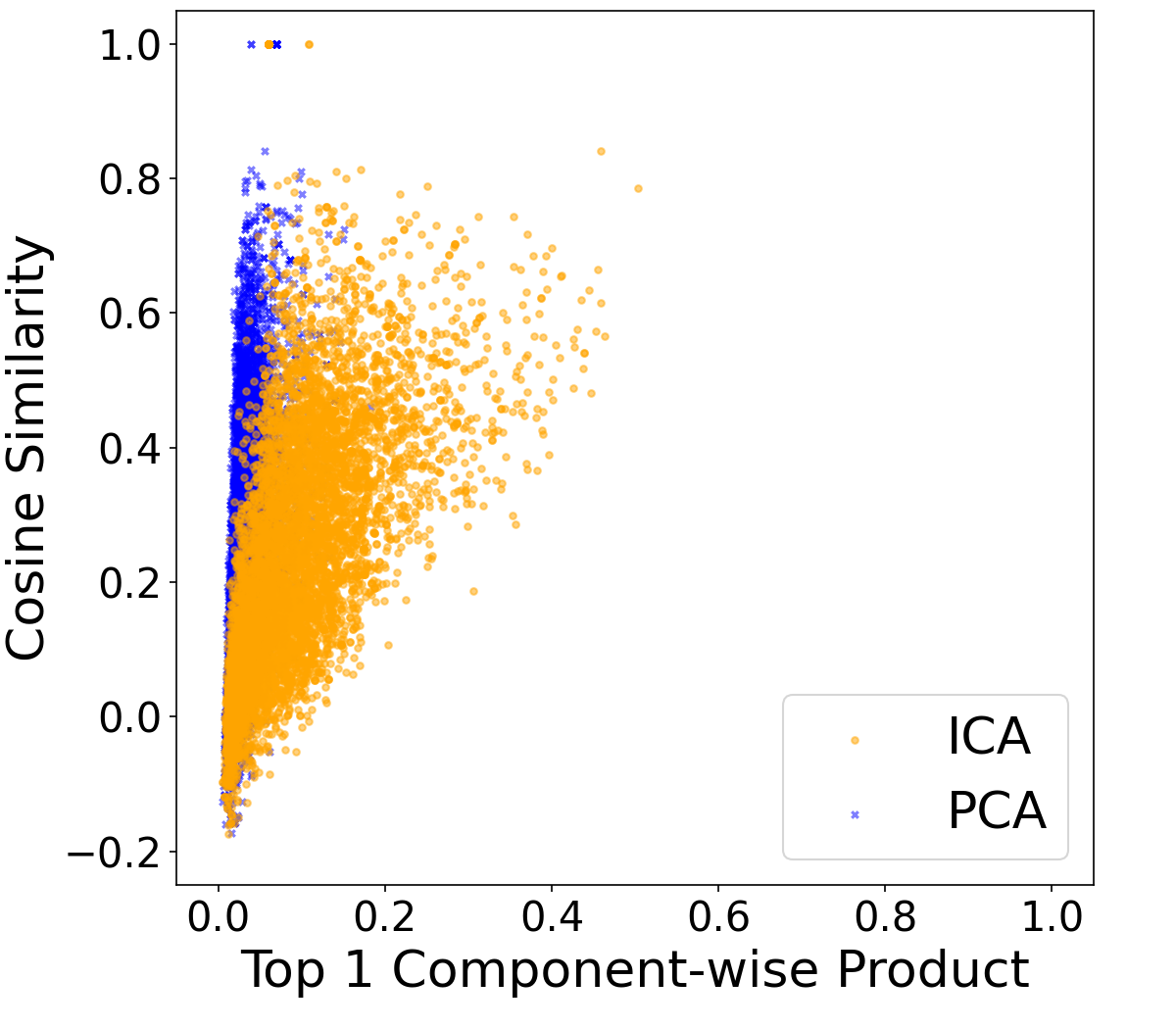
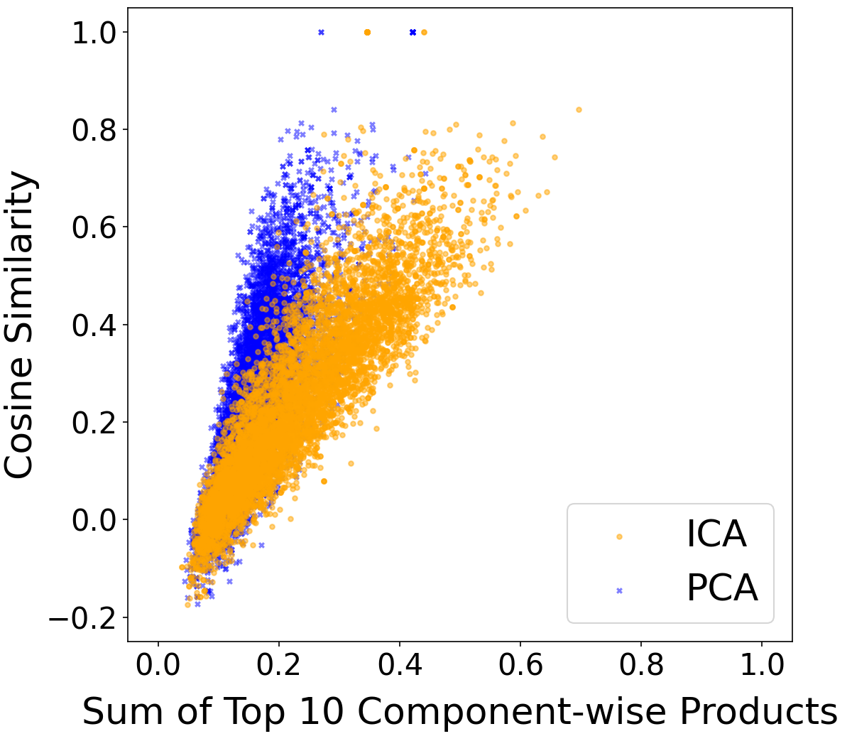
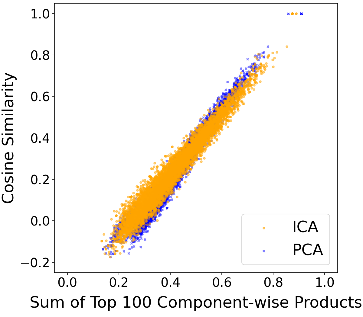
Figure 22 shows the comparison of the scatterplots for the sum and the cosine similarity for the normalized ICA-transformed and PCA-transformed embeddings. For smaller values of $p$, such as $p=1$ or $p=10$, the correlation of the scatterplots is stronger for ICA than for PCA. At $p=100$, the scatterplot shows strong correlations for both ICA and PCA.

Figure 23 compares the correlation coefficients at different values of $p$ for these normalized embeddings. As seen in Fig. 22, the correlation coefficients for ICA are stronger than those for PCA at smaller values of $p$. As $p$ increases, the correlation coefficients for both ICA and PCA increase and the difference between them decreases. These results indicate the favorable sparsity of the component-wise products of the normalized ICA-transformed embeddings.

References

- Alvarez-Melis and Jaakkola (2018) David Alvarez-Melis and Tommi S. Jaakkola. 2018. Gromov-wasserstein alignment of word embedding spaces. In Proceedings of the 2018 Conference on Empirical Methods in Natural Language Processing, Brussels, Belgium, October 31 - November 4, 2018, pages 1881–1890. Association for Computational Linguistics.
- Arefyev et al. (2018) Nikolay Arefyev, Pavel Ermolaev, and Alexander Panchenko. 2018. How much does a word weigh? weighting word embeddings for word sense induction. CoRR, abs/1805.09209.
- Bojanowski et al. (2017) Piotr Bojanowski, Edouard Grave, Armand Joulin, and Tomás Mikolov. 2017. Enriching word vectors with subword information. Trans. Assoc. Comput. Linguistics, 5:135–146.
- Bommasani et al. (2020) Rishi Bommasani, Kelly Davis, and Claire Cardie. 2020. Interpreting pretrained contextualized representations via reductions to static embeddings. In Proceedings of the 58th Annual Meeting of the Association for Computational Linguistics, ACL 2020, Online, July 5-10, 2020, pages 4758–4781. Association for Computational Linguistics.
- Bruni et al. (2014) Elia Bruni, Nam-Khanh Tran, and Marco Baroni. 2014. Multimodal distributional semantics. Journal of Artificial Intelligence Research, 49:1–47.
- Chagnaa et al. (2007) Altangerel Chagnaa, Cheol-Young Ock, Chang-Beom Lee, and Purev Jaimai. 2007. Feature extraction of concepts by independent component analysis. Journal of Information Processing Systems, 3(1):33–37.
- Deng et al. (2019) Jiankang Deng, Jia Guo, Niannan Xue, and Stefanos Zafeiriou. 2019. Arcface: Additive angular margin loss for deep face recognition. In IEEE Conference on Computer Vision and Pattern Recognition, CVPR 2019, Long Beach, CA, USA, June 16-20, 2019, pages 4690–4699. Computer Vision Foundation / IEEE.
- Faruqui et al. (2015) Manaal Faruqui, Yulia Tsvetkov, Dani Yogatama, Chris Dyer, and Noah A. Smith. 2015. Sparse overcomplete word vector representations. In Proceedings of the 53rd Annual Meeting of the Association for Computational Linguistics and the 7th International Joint Conference on Natural Language Processing of the Asian Federation of Natural Language Processing, ACL 2015, July 26-31, 2015, Beijing, China, Volume 1: Long Papers, pages 1491–1500. The Association for Computer Linguistics.
- Finkelstein et al. (2002) Lev Finkelstein, Evgeniy Gabrilovich, Yossi Matias, Ehud Rivlin, Zach Solan, Gadi Wolfman, and Eytan Ruppin. 2002. Placing search in context: The concept revisited. ACM Transactions on information systems, 20(1):116–131.
- Gao et al. (2021) Tianyu Gao, Xingcheng Yao, and Danqi Chen. 2021. Simcse: Simple contrastive learning of sentence embeddings. In Proceedings of the 2021 Conference on Empirical Methods in Natural Language Processing, EMNLP 2021, Virtual Event / Punta Cana, Dominican Republic, 7-11 November, 2021, pages 6894–6910. Association for Computational Linguistics.
- Hill et al. (2015) Felix Hill, Roi Reichart, and Anna Korhonen. 2015. Simlex-999: Evaluating semantic models with (genuine) similarity estimation. Computational Linguistics, 41(4):665–695.
- Hotelling (1933) Harold Hotelling. 1933. Analysis of a complex of statistical variables into principal components. Journal of educational psychology, 24(6):417.
- Huben et al. (2024) Robert Huben, Hoagy Cunningham, Logan Riggs Smith, Aidan Ewart, and Lee Sharkey. 2024. Sparse autoencoders find highly interpretable features in language models. In The Twelfth International Conference on Learning Representations.
- Hyvärinen (1999) Aapo Hyvärinen. 1999. Fast and robust fixed-point algorithms for independent component analysis. IEEE Trans. Neural Networks, 10(3):626–634.
- Hyvärinen and Oja (2000) Aapo Hyvärinen and Erkki Oja. 2000. Independent component analysis: algorithms and applications. Neural Networks, 13(4-5):411–430.
- Ishibashi et al. (2020) Yoichi Ishibashi, Katsuhito Sudoh, Koichiro Yoshino, and Satoshi Nakamura. 2020. Reflection-based word attribute transfer. In Proceedings of the 58th Annual Meeting of the Association for Computational Linguistics: Student Research Workshop, ACL 2020, Online, July 5-10, 2020, pages 51–58. Association for Computational Linguistics.
- Jastrzebski et al. (2017) Stanislaw Jastrzebski, Damian Lesniak, and Wojciech Marian Czarnecki. 2017. How to evaluate word embeddings? on importance of data efficiency and simple supervised tasks. CoRR, abs/1702.02170.
- Kobayashi et al. (2020) Goro Kobayashi, Tatsuki Kuribayashi, Sho Yokoi, and Kentaro Inui. 2020. Attention is not only a weight: Analyzing transformers with vector norms. In Proceedings of the 2020 Conference on Empirical Methods in Natural Language Processing, EMNLP 2020, Online, November 16-20, 2020, pages 7057–7075. Association for Computational Linguistics.
- Kurita et al. (2023) Hiroto Kurita, Goro Kobayashi, Sho Yokoi, and Kentaro Inui. 2023. Contrastive learning-based sentence encoders implicitly weight informative words. In Findings of the Association for Computational Linguistics: EMNLP 2023, Singapore, December 6-10, 2023, pages 10932–10947. Association for Computational Linguistics.
- Lample et al. (2018) Guillaume Lample, Alexis Conneau, Marc’Aurelio Ranzato, Ludovic Denoyer, and Hervé Jégou. 2018. Word translation without parallel data. In 6th International Conference on Learning Representations, ICLR 2018, Vancouver, BC, Canada, April 30 - May 3, 2018, Conference Track Proceedings. OpenReview.net.
- Li and Han (2013) Baoli Li and Liping Han. 2013. Distance weighted cosine similarity measure for text classification. In Intelligent Data Engineering and Automated Learning - IDEAL 2013 - 14th International Conference, IDEAL 2013, Hefei, China, October 20-23, 2013. Proceedings, volume 8206 of Lecture Notes in Computer Science, pages 611–618. Springer.
- Li and Li (2023) Xianming Li and Jing Li. 2023. Angle-optimized text embeddings. CoRR, abs/2309.12871.
- Liang et al. (2021) Yuxin Liang, Rui Cao, Jie Zheng, Jie Ren, and Ling Gao. 2021. Learning to remove: Towards isotropic pre-trained BERT embedding. In Artificial Neural Networks and Machine Learning - ICANN 2021 - 30th International Conference on Artificial Neural Networks, Bratislava, Slovakia, September 14-17, 2021, Proceedings, Part V, volume 12895 of Lecture Notes in Computer Science, pages 448–459. Springer.
- Luo et al. (2015) Hongyin Luo, Zhiyuan Liu, Huan-Bo Luan, and Maosong Sun. 2015. Online learning of interpretable word embeddings. In Proceedings of the 2015 Conference on Empirical Methods in Natural Language Processing, EMNLP 2015, Lisbon, Portugal, September 17-21, 2015, pages 1687–1692. The Association for Computational Linguistics.
- Luong et al. (2013) Thang Luong, Richard Socher, and Christopher Manning. 2013. Better word representations with recursive neural networks for morphology. In Proceedings of the Seventeenth Conference on Computational Natural Language Learning, pages 104–113.
- Mareček et al. (2020) David Mareček, Jindřich Libovický, Tomáš Musil, Rudolf Rosa, and Tomasz Limisiewicz. 2020. Hidden in the Layers: Interpretation of Neural Networks for Natural Language Processing, volume 20 of Studies in Computational and Theoretical Linguistics. Institute of Formal and Applied Linguistics, Prague, Czechia.
- Mikolov et al. (2013a) Tomás Mikolov, Kai Chen, Greg Corrado, and Jeffrey Dean. 2013a. Efficient estimation of word representations in vector space. In 1st International Conference on Learning Representations, ICLR 2013, Scottsdale, Arizona, USA, May 2-4, 2013, Workshop Track Proceedings.
- Mikolov et al. (2013b) Tomás Mikolov, Quoc V. Le, and Ilya Sutskever. 2013b. Exploiting similarities among languages for machine translation. CoRR, abs/1309.4168.
- Mikolov et al. (2013c) Tomás Mikolov, Ilya Sutskever, Kai Chen, Gregory S. Corrado, and Jeffrey Dean. 2013c. Distributed representations of words and phrases and their compositionality. In Advances in Neural Information Processing Systems 26: 27th Annual Conference on Neural Information Processing Systems 2013. Proceedings of a meeting held December 5-8, 2013, Lake Tahoe, Nevada, United States, pages 3111–3119.
- Mikolov et al. (2013d) Tomás Mikolov, Wen-tau Yih, and Geoffrey Zweig. 2013d. Linguistic regularities in continuous space word representations. In Human Language Technologies: Conference of the North American Chapter of the Association of Computational Linguistics, Proceedings, June 9-14, 2013, Westin Peachtree Plaza Hotel, Atlanta, Georgia, USA, pages 746–751. The Association for Computational Linguistics.
- Murphy et al. (2012) Brian Murphy, Partha Pratim Talukdar, and Tom M. Mitchell. 2012. Learning effective and interpretable semantic models using non-negative sparse embedding. In COLING 2012, 24th International Conference on Computational Linguistics, Proceedings of the Conference: Technical Papers, 8-15 December 2012, Mumbai, India, pages 1933–1950. Indian Institute of Technology Bombay.
- Musil (2019) Tomás Musil. 2019. Examining structure of word embeddings with PCA. In Text, Speech, and Dialogue - 22nd International Conference, TSD 2019, Ljubljana, Slovenia, September 11-13, 2019, Proceedings, volume 11697 of Lecture Notes in Computer Science, pages 211–223. Springer.
- Musil and Mareček (2022) Tomás Musil and David Mareček. 2022. Independent components of word embeddings represent semantic features. CoRR, abs/2212.09580.
- Nadarajah and Pogány (2016) Saralees Nadarajah and Tibor K. Pogány. 2016. On the distribution of the product of correlated normal random variables. Comptes Rendus Mathematique, 354(2):201–204.
- Nagata et al. (2023) Ryo Nagata, Hiroya Takamura, Naoki Otani, and Yoshifumi Kawasaki. 2023. Variance matters: Detecting semantic differences without corpus/word alignment. In Proceedings of the 2023 Conference on Empirical Methods in Natural Language Processing, EMNLP 2023, Singapore, December 6-10, 2023, pages 15609–15622. Association for Computational Linguistics.
- Oyama et al. (2023) Momose Oyama, Sho Yokoi, and Hidetoshi Shimodaira. 2023. Norm of word embedding encodes information gain. In Proceedings of the 2023 Conference on Empirical Methods in Natural Language Processing, EMNLP 2023, Singapore, December 6-10, 2023, pages 2108–2130. Association for Computational Linguistics.
- Pagliardini et al. (2018) Matteo Pagliardini, Prakhar Gupta, and Martin Jaggi. 2018. Unsupervised learning of sentence embeddings using compositional n-gram features. In Proceedings of the 2018 Conference of the North American Chapter of the Association for Computational Linguistics: Human Language Technologies, NAACL-HLT 2018, New Orleans, Louisiana, USA, June 1-6, 2018, Volume 1 (Long Papers), pages 528–540. Association for Computational Linguistics.
- Park et al. (2017) Sungjoon Park, JinYeong Bak, and Alice Oh. 2017. Rotated word vector representations and their interpretability. In Proceedings of the 2017 Conference on Empirical Methods in Natural Language Processing, EMNLP 2017, Copenhagen, Denmark, September 9-11, 2017, pages 401–411. Association for Computational Linguistics.
- Pedregosa et al. (2011) Fabian Pedregosa, Gaël Varoquaux, Alexandre Gramfort, Vincent Michel, Bertrand Thirion, Olivier Grisel, Mathieu Blondel, Peter Prettenhofer, Ron Weiss, Vincent Dubourg, Jake VanderPlas, Alexandre Passos, David Cournapeau, Matthieu Brucher, Matthieu Perrot, and Edouard Duchesnay. 2011. Scikit-learn: Machine learning in python. J. Mach. Learn. Res., 12:2825–2830.
- Pennington et al. (2014) Jeffrey Pennington, Richard Socher, and Christopher D. Manning. 2014. Glove: Global vectors for word representation. In Proceedings of the 2014 Conference on Empirical Methods in Natural Language Processing, EMNLP 2014, October 25-29, 2014, Doha, Qatar, A meeting of SIGDAT, a Special Interest Group of the ACL, pages 1532–1543. ACL.
- Radinsky et al. (2011) Kira Radinsky, Eugene Agichtein, Evgeniy Gabrilovich, and Shaul Markovitch. 2011. A word at a time: Computing word relatedness using temporal semantic analysis. In Proceedings of the 20th International Conference on World Wide Web, page 337–346.
- Reimers and Gurevych (2019) Nils Reimers and Iryna Gurevych. 2019. Sentence-bert: Sentence embeddings using siamese bert-networks. In Proceedings of the 2019 Conference on Empirical Methods in Natural Language Processing and the 9th International Joint Conference on Natural Language Processing, EMNLP-IJCNLP 2019, Hong Kong, China, November 3-7, 2019, pages 3980–3990. Association for Computational Linguistics.
- Rubenstein and Goodenough (1965) Herbert Rubenstein and John B. Goodenough. 1965. Contextual correlates of synonymy. Commun. ACM, 8(10):627–633.
- Sasaki et al. (2023) Shota Sasaki, Benjamin Heinzerling, Jun Suzuki, and Kentaro Inui. 2023. Examining the effect of whitening on static and contextualized word embeddings. Inf. Process. Manag., 60(3):103272.
- Schakel and Wilson (2015) Adriaan M. J. Schakel and Benjamin J. Wilson. 2015. Measuring word significance using distributed representations of words. CoRR, abs/1508.02297.
- Schnabel et al. (2015) Tobias Schnabel, Igor Labutov, David M. Mimno, and Thorsten Joachims. 2015. Evaluation methods for unsupervised word embeddings. In Proceedings of the 2015 Conference on Empirical Methods in Natural Language Processing, EMNLP 2015, Lisbon, Portugal, September 17-21, 2015, pages 298–307. The Association for Computational Linguistics.
- Shin et al. (2018) Jamin Shin, Andrea Madotto, and Pascale Fung. 2018. Interpreting word embeddings with eigenvector analysis. In 32nd Conference on Neural Information Processing Systems (NIPS 2018), IRASL workshop, pages 73–81.
- Sitikhu et al. (2019) Pinky Sitikhu, Kritish Pahi, Pujan Thapa, and Subarna Shakya. 2019. A comparison of semantic similarity methods for maximum human interpretability. In 2019 artificial intelligence for transforming business and society (AITB), volume 1, pages 1–4. IEEE.
- Steck et al. (2024) Harald Steck, Chaitanya Ekanadham, and Nathan Kallus. 2024. Is cosine-similarity of embeddings really about similarity? CoRR, abs/2403.05440.
- Su et al. (2021) Jianlin Su, Jiarun Cao, Weijie Liu, and Yangyiwen Ou. 2021. Whitening sentence representations for better semantics and faster retrieval. CoRR, abs/2103.15316.
- Subramanian et al. (2018) Anant Subramanian, Danish Pruthi, Harsh Jhamtani, Taylor Berg-Kirkpatrick, and Eduard H. Hovy. 2018. SPINE: sparse interpretable neural embeddings. In Proceedings of the Thirty-Second AAAI Conference on Artificial Intelligence, (AAAI-18), the 30th innovative Applications of Artificial Intelligence (IAAI-18), and the 8th AAAI Symposium on Educational Advances in Artificial Intelligence (EAAI-18), New Orleans, Louisiana, USA, February 2-7, 2018, pages 4921–4928. AAAI Press.
- Sun et al. (2016) Fei Sun, Jiafeng Guo, Yanyan Lan, Jun Xu, and Xueqi Cheng. 2016. Sparse word embeddings using regularized online learning. In Proceedings of the Twenty-Fifth International Joint Conference on Artificial Intelligence, IJCAI 2016, New York, NY, USA, 9-15 July 2016, pages 2915–2921. IJCAI/AAAI Press.
- Sundararajan et al. (2017) Mukund Sundararajan, Ankur Taly, and Qiqi Yan. 2017. Axiomatic attribution for deep networks. In Proceedings of the 34th International Conference on Machine Learning, ICML 2017, Sydney, NSW, Australia, 6-11 August 2017, volume 70 of Proceedings of Machine Learning Research, pages 3319–3328. PMLR.
- van Dongen and Enright (2012) Stijn van Dongen and Anton J. Enright. 2012. Metric distances derived from cosine similarity and pearson and spearman correlations. CoRR, abs/1208.3145.
- Xia et al. (2015) Peipei Xia, Li Zhang, and Fanzhang Li. 2015. Learning similarity with cosine similarity ensemble. Inf. Sci., 307:39–52.
- Xing et al. (2015) Chao Xing, Dong Wang, Chao Liu, and Yiye Lin. 2015. Normalized word embedding and orthogonal transform for bilingual word translation. In NAACL HLT 2015, The 2015 Conference of the North American Chapter of the Association for Computational Linguistics: Human Language Technologies, Denver, Colorado, USA, May 31 - June 5, 2015, pages 1006–1011. The Association for Computational Linguistics.
- Yamagiwa et al. (2023) Hiroaki Yamagiwa, Momose Oyama, and Hidetoshi Shimodaira. 2023. Discovering universal geometry in embeddings with ICA. In Proceedings of the 2023 Conference on Empirical Methods in Natural Language Processing, EMNLP 2023, Singapore, December 6-10, 2023, pages 4647–4675. Association for Computational Linguistics.
- Yamagiwa et al. (2024) Hiroaki Yamagiwa, Yusuke Takase, and Hidetoshi Shimodaira. 2024. Axis tour: Word tour determines the order of axes in ica-transformed embeddings. CoRR, abs/2401.06112.
- Yokoi et al. (2020) Sho Yokoi, Ryo Takahashi, Reina Akama, Jun Suzuki, and Kentaro Inui. 2020. Word rotator’s distance. In Proceedings of the 2020 Conference on Empirical Methods in Natural Language Processing, EMNLP 2020, Online, November 16-20, 2020, pages 2944–2960. Association for Computational Linguistics.
- Zhang et al. (2020) Tianyi Zhang, Varsha Kishore, Felix Wu, Kilian Q. Weinberger, and Yoav Artzi. 2020. Bertscore: Evaluating text generation with BERT. In 8th International Conference on Learning Representations, ICLR 2020, Addis Ababa, Ethiopia, April 26-30, 2020. OpenReview.net.