Graph Neural Thompson Sampling

Abstract

We consider an online decision-making problem with a reward function defined over graph-structured data. We formally formulate the problem as an instance of graph action bandit. We then propose GNN-TS, a Graph Neural Network (GNN) powered Thompson Sampling (TS) algorithm which employs a GNN approximator for estimating the mean reward function and the graph neural tangent features for uncertainty estimation. We prove that, under certain boundness assumptions on the reward function, GNN-TS achieves a state-of-the-art regret bound which is (1) sub-linear of order $\tilde{{\mathcal{O}}}((\tilde{d}T)^{1/2})$ in the number of interaction rounds, $T$, and a notion of effective dimension $\tilde{d}$, and (2) independent of the number of graph nodes. Empirical results validate that our proposed GNN-TS exhibits competitive performance and scales well on graph action bandit problems.

1 Introduction

Thompson Sampling [Thompson, 1933] is a widely adopted and effective technique in sequential decision-making problems, known for its ease of implementation and practical success [Chapelle and Li, 2011, Kawale et al., 2015, Russo et al., 2018, Riquelme et al., 2018]. The fundamental concept behind Thompson Sampling (TS) is to compute the posterior probability of each action being optimal for the present context, followed by the selection of an action from this distribution. Previous research has extended TS or developed variants of it to incorporate increasingly complex models of the reward function, such as Linear TS [Agrawal and Goyal, 2013, Abeille and Lazaric, 2017], Kernelized TS [Chowdhury and Gopalan, 2017], and Neural TS [Zhang et al., 2020]. However, these efforts have mainly focused on conventional data types. In contrast, the application of sequential learning to graph-structured data, such as molecular or biological graph representations, introduces unique challenges that merit further investigation.

Recently, there has been a growing interest in studying bandit optimization over graphs. Several researchers have initiated this line of work by addressing the challenge of encoding graph structures in bandit problems [Gómez-Bombarelli et al., 2018, Jin et al., 2018, Griffiths and Hernández-Lobato, 2020, Korovina et al., 2020]. More recently, Graph Neural Network (GNN) bandits have been proposed, which leverage expressive GNNs to approximate reward functions on graphs [Kassraie et al., 2022]. Despite these advancements, the GNN bandits remain relatively unexplored compared to the extensive research on Neural bandits. Firstly, a formal formulation of this sequential graph selection problem is yet to be proposed. More importantly, there is a significant lack of comprehensive theoretical and empirical investigations regarding the use of TS in sequential graph selection.

Contribution. In this work, we address the online decision-making problem over graph-structured data by contributing a novel algorithm called GNN-TS. We begin by formulating the sequential graph selection as graph action bandit. We then propose Graph Neural Thompson Sampling, GNN-TS, to incorporate TS exploration with graph neural networks. We establish a regret bound for the proposed algorithm with sub-linear growth of order $\tilde{{\mathcal{O}}}((\tilde{d}T)^{1/2})$ with respect to the effective dimension $\tilde{d}$ and the number of interaction round $T$, and independent of the number of graph nodes. Finally, we corroborate the analysis with an empirical evaluation of the algorithm in simulations. Experiments show that GNN-TS yields competitive performance and scalability, compared to the state-of-the-art baselines, underscoring its practical value in addition to its strong theoretical guarantees.

Notations. Let $[n]=\{1,2,...,n\}$. For a set or event ${\mathcal{E}}$, we denote its complement as $\bar{{\mathcal{E}}}$. ${\boldsymbol{I}}_{n}\in\mathbb{R}^{n\times n}$ is the identity matrix. For a matrix ${\boldsymbol{A}}$, ${\boldsymbol{A}}_{i*}$ and ${\boldsymbol{A}}_{*j}$ denote its $i$-th row and $j$-th column, respectively. $\lambda_{\max}({\boldsymbol{A}})$ and $\lambda_{\min}({\boldsymbol{A}})$ represents the maximum and minimum eigenvalues of the matrix ${\boldsymbol{A}}$. For any vector ${\boldsymbol{x}}$ and square matrix ${\boldsymbol{A}}$, $\|{\boldsymbol{x}}\|_{{\boldsymbol{A}}}=\sqrt{{\boldsymbol{x}}^{\top}{\boldsymbol{A}}{\boldsymbol{x}}}$. We denote the history of randomness up to (but not including) round $t$ as ${\mathcal{F}}_{t}$ and write $\mathbb{P}_{t}(\cdot):=\mathbb{P}(\,\cdot\,\,|\,{\mathcal{F}}_{t})$ and $\mathbb{E}_{t}(\cdot):=\mathbb{E}[\,\cdot\,\,|\,{\mathcal{F}}_{t}]$ for the conditional probability and expectation given ${\mathcal{F}}_{t}$. We use $\lesssim$ and big-$O$, to denote “less than”, up to a constant factor. We further use $\tilde{{\mathcal{O}}}(\cdot)$ for big-$O$ up to logarithmic factor.

2 Related Works

Graph Bandit. Multiple works have studied graph bandit problems, which can be classified into two categories: graph as structure across arms and graph as data. Most research focuses on the former category, starting from spectral bandit [Kocák et al., 2014, 2020] to graphical bandit [Liu et al., 2018, Yu et al., 2020, Gou et al., 2023, Toni and Frossard, 2023]. Within this field, bandit problems with graph feedback have garnered significant attention [Tossou et al., 2017, Dann et al., 2020, Chen et al., 2021, Kong et al., 2022], where learners observe rewards from selected nodes and their neighborhoods. The primary focus of these works have been improving sample efficiency [Bellemare et al., 2019, Waradpande et al., 2020, Idé et al., 2022], with some assuming that payoffs are shared according to the graph Laplacian [Esposito et al., 2022, Lee et al., 2020, Lykouris et al., 2020, Thaker et al., 2022, Yang et al., 2020]. While the existing literature primarily aims to optimize over geometrical signal domains, our work focuses on optimization within graph domains. Specifically, we investigate the online graph selection problem, aligning with the second category of research that considers the entire graph as input data. A related recent work [Kassraie et al., 2022] proposed a GNN bandit approach with regret bound based on information gain and an elimination-based algorithm. In contrast, our work explores regret bound based on the effective dimension and builds upon the foundation of Thompson Sampling. This second category of research also encompasses empirical works [Upadhyay et al., 2020, Qi et al., 2022, 2023], particularly those centered around molecule optimization [Wang-Henderson et al., 2023a, b].

Neural Bandit. Our work contributes to the research on neural bandits, where deep neural networks are utilized to estimate the reward function. The work of Zahavy and Mannor [2019], Xu et al. [2020] investigated the Neural Linear bandit, while Zhou et al. [2020] developed Neural Upper Confidence Bound (UCB), an extension of Linear UCB. Zhang et al. [2020] adapted TS with deep neural networks, proposing Neural TS. Dai et al. [2022] makes improvements to neural bandit algorithms to overcome practical limitations. Nguyen-Tang et al. [2021] explores neural bandit in an offline contextual bandit setting and  [Gu et al., 2024] examines batched learning for neural bandit. Our work can be seen as an extension of Neural TS [Zhang et al., 2020], incorporating significant improvements such as the utilization of graph neural tangent kernel and a distinct definition of effective dimension.

3 Problem Formulation and Methodology

3.1 Graph Action Bandit Problem

We consider an online decision-making problem in which the learner aims to optimize an unknown reward function by sequentially interacting with a stochastic environment. We identify the actions with graphs from an action space ${\mathcal{G}}$ and assume that the size of this action space, denoted as $|\mathcal{G}|$, is finite. At time $t\in[T]$, the learner selects a graph $G_{t}$ from the action space ${\mathcal{G}}_{t}\subset{\mathcal{G}}$. The learner then observes a noisy reward $y_{t}=\mu(G_{t})+\varepsilon_{t}$ where $\mu:{\mathcal{G}}\rightarrow\mathbb{R}$ is the true (unknown) reward function and $\{\varepsilon_{t}\}_{t\in[T]}$ are i.i.d zero-mean sub-gaussian noise with variance proxy $\sigma^{2}_{\varepsilon}$. The goal of the learner is to maximize the expected cumulative reward in $T$ rounds, which equivalently entails minimizing the expected (pseudo-)regret denoted as $R_{T}=\sum_{t=1}^{T}\mathbb{E}[\mu(G^{*}_{t})-\mu(G_{t})]$ where $G^{*}_{t}=\operatorname*{argmax}_{G\in{\mathcal{G}}_{t}}\mu(G)$ represents the optimal graph at time $t$.

The graph space ${\mathcal{G}}$ is a finite set of undirected graphs with at most $N$ nodes. Note that the graphs with less than $N$ nodes can be treated by adding auxiliary isolated nodes with no features. We denote an undirected attributed graph with $N$ nodes as $G=(\mathbf{X},\mathbf{A})$, where $\mathbf{X}\in\mathbb{R}^{N\times d}$ represents the feature matrix with $d$ features, and $\mathbf{A}\in\{0,1\}^{N\times N}$ is the unweighted adjacency matrix. The rows of $\mathbf{X}$ correspond to node features. The size of the node set of a graph $G$ is denoted as $|\mathcal{V}(G)|\leq N$.

Graph action bandit has several applications such as chemical molecules optimization. Consider the graph structures representing the molecules [Weininger, 1988] and rewards are molecular properties. The goal is to sequentially recommend the optimal molecules for experimental testing.

3.2 Graph Neural Network Model

We propose to learn the unknown reward function $\mu(\cdot)$ by fitting a Graph Neural Network (GNN). We consider a relatively simple GNN architecture where the output of a single graph convolution layer is normalized (to unit $\ell_{2}$ norm) and passed through a multilayer perceptron (MLP). A single-layer graph convolution can be compactly stated as ${\boldsymbol{A}}{\boldsymbol{X}}$ using the adjacency matrix ${\boldsymbol{A}}$ of the network. Additionally, we normalize each row of the resulting matrix to have a unit $\ell_{2}$ norm. Letting $u({\boldsymbol{x}})={\boldsymbol{x}}/\|{\boldsymbol{x}}\|_{2}$ denote the normalization operator, the aggregated feature of node $i$ in a graph $G$ is ${\boldsymbol{h}}_{i}^{G}=u(({\boldsymbol{A}}{\boldsymbol{X}})_{i*})=u(\sum_{j\in{\mathcal{N}}_{i}}{\boldsymbol{X}}_{j*})$ where ${\mathcal{N}}_{j}$ is the neighborhood of node $j$. Our GNN also consists of an $L$-layer $m$-width MLP neural network $f_{\operatorname{MLP}}$ which is defined recursively as follows

$$f^{(1)}({\boldsymbol{h}}_{i}^{G}) ={\boldsymbol{W}}^{(1)}{\boldsymbol{h}}_{i}^{G},\quad i\in[N],$$ (1)

$$f^{(l)}({\boldsymbol{h}}_{i}^{G}) =\frac{1}{\sqrt{m}}{\boldsymbol{W}}^{(l)}{\mbox{ReLU}}(f^{(l-1)}({\boldsymbol{h}}_{i}^{G})),\quad 2\leq l\leq L,$$

$$f_{\operatorname{MLP}}({\boldsymbol{h}}_{i}^{G};{\boldsymbol{\theta}}) =f^{(L)}({\boldsymbol{h}}_{i}^{G}).$$

Here, ${\mbox{ReLU}}(\cdot)=\max(\cdot,0)$, ${\boldsymbol{W}}^{(1)}\in\mathbb{R}^{m\times d}$, ${\boldsymbol{W}}^{(L)}\in\mathbb{R}^{1\times m}$, ${\boldsymbol{W}}^{(l)}\in\mathbb{R}^{m\times m}$ for any $1<l<L$ are weight matrices of the MLP and ${\boldsymbol{\theta}}:=({\boldsymbol{W}}^{(1)},\dots,{\boldsymbol{W}}^{(L)})\in\mathbb{R}^{p}$ is the collection of parameters of the neural network where $p=dm+(L-2)m^{2}+m$. Our GNN model to estimate the reward function is

$$f_{\operatorname{GNN}}(G;{\boldsymbol{\theta}}):=\frac{1}{N}\sum_{i=1}^{N}f_{\operatorname{MLP}}({\boldsymbol{h}}_{i}^{G};{\boldsymbol{\theta}}).$$ (2)

The gradient of ${\boldsymbol{\theta}}\mapsto f_{\operatorname{GNN}}(G;{\boldsymbol{\theta}})$ denoted as ${\boldsymbol{\textnormal{{g}}}}(G;{\boldsymbol{\theta}}):=\nabla_{{\boldsymbol{\theta}}}f_{\operatorname{GNN}}(G;{\boldsymbol{\theta}})$ will play a key role in uncertainty quantification, which will be discussed in Section 3.3. The GNN model (2) is trained by minimizing the mean-squared loss with $\ell_{2}$ penalty, described concretely in (6). A hyperparameter $\lambda$ is used to tune the strength of $\ell_{2}$ regularization. For the simplicity of exposition, in the theoretical analysis, we solve the optimization via gradient descent with learning rate $\eta$, total number of iterations $J$ and initialize parameters ${\boldsymbol{\theta}}_{0}$ such that $f_{\operatorname{GNN}}(G;{\boldsymbol{\theta}}_{0})=0$ for all $G\in{\mathcal{G}}$, which can be fulfilled based on the work of Zhou et al. [2020], Kassraie and Krause [2022].

3.3 Graph Neural Thompson Sampling

We adapt Thompson Sampling (TS) for graph exploration, due to its robust performance in balancing exploration against exploitation. Algorithm 1 outlines our proposed GNN Thompson sampling, following the idea of NeuralTS in Zhang et al. [2020]. The key step is the sampling of an estimated reward mean $\widehat{r}_{t}(G)$ for each graph $G$ in the action space at time $t$, from a normal distribution as in equation (4). The mean of the normal distribution in (4) is our current estimate, $f_{\operatorname{GNN}}(G;{\boldsymbol{\theta}}_{t-1})$, of the true mean reward for graph $G$ (i.e., $\mu(G)$). This estimate is obtained by fitting the GNN to all the past data as in (6). The variance of the normal distribution $\nu^{2}\sigma_{t}^{2}(G)$ is our current measure of uncertainty about the true reward of graph $G$. Note that

$$\sigma^{2}_{t}(G)=\frac{1}{m}\|{\boldsymbol{\textnormal{{g}}}}(G;{\boldsymbol{\theta}}_{t-1})\|_{{\boldsymbol{U}}_{t-1}^{-1}}^{2}\quad\text{where}\quad{\boldsymbol{U}}_{t-1}=\lambda{\boldsymbol{I}}_{p}+\frac{1}{m}\sum_{i=1}^{t-1}{\boldsymbol{\textnormal{{g}}}}(G_{i};{\boldsymbol{\theta}}_{i-1}){\boldsymbol{\textnormal{{g}}}}(G_{i};{\boldsymbol{\theta}}_{i-1})^{\top}.$$ (3)

The rationale behind $\sigma_{t}^{2}(G)$ comes from a linear approximation to $f_{\operatorname{GNN}}(G;{\boldsymbol{\theta}})$. In particular, the idea is that (6) approximately looks like a linear ridge regression problem, with features $\{{\boldsymbol{\textnormal{{g}}}}(G_{i};{\boldsymbol{\theta}}_{i})/\sqrt{m}\}_{i\in[t]}$. The expression (3) is then the familiar estimated covariance matrix from linear bandits after we make this identification. This approximation can be made rigorous via the neural tangent kernel idea, as discussed in Section 4.

The sampled reward mean $\widehat{r}_{t}(G)$ is the index for decision-making. The learner selects the graph with the highest index, i.e., $G_{t}=\operatorname*{argmax}_{G\in{\mathcal{G}}}\widehat{r}_{t}(G)$. The randomness in $\widehat{r}_{t}(G)$, due to the positive variance of the sampling distribution, is what allows TS to efficiently explore the action space. We want the uncertainty, as captured by $\sigma_{t}^{2}(G)$ not to be too small early on, to allow for effective exploration, but not too large either to miss out on the optimal choice too often. Lemma 5.2 in Section 5 captures the two sides of this trade-off in our theory.

It is worth noting that our proposed Algorithm 1 is not exact TS. In our approach, (4) serves as an approximation to a posterior for mean reward function, rather than a true posterior. The difference between our proposed method and an exact Bayesian method will be smaller if the GNN model is better approximated by a linear model.

Lastly, we note that $\widehat{r}_{t}(G)$ is also referred to as the perturbed mean reward, as it can be expressed as: $\widehat{r}_{t}(G)=f_{\operatorname{GNN}}(G;{\boldsymbol{\theta}}_{t-1})+\nu\sigma_{t}(G)z$ where $z\sim{\mathcal{N}}(0,1)$. This perturbed reward includes both the estimated part ($f_{\text{gnn}}(G;\boldsymbol{\theta}_{t-1})$) and the random perturbation part ($\nu\sigma_{t}(G)\cdot z$). The use of perturbations for exploration has been shown to be a strong strategy in previous works [Kim and Tewari, 2019, Kveton et al., 2019a]. Algorithm 1 can be summarized as greedily selecting the graph with the highest perturbed mean reward.

Algorithm 1 Graph Neural Thompson Sampling (GNN-TS)

1:Input: $T$, $\lambda$, $\nu$

2:Initialization: ${\boldsymbol{\theta}}_{0}$, ${\boldsymbol{U}}_{0}=\lambda{\boldsymbol{I}}_{p}$.

3:for $t=1,...,T$ do

4:     Compute $\sigma_{t}^{2}(G):=\frac{1}{m}\|{\boldsymbol{\textnormal{{g}}}}(G;{\boldsymbol{\theta}}_{t-1})\|_{{\boldsymbol{U}}_{t-1}^{-1}}^{2}$ and sample

$$\widehat{r}_{t}(G)\sim{\mathcal{N}}\bigl{(}f_{\operatorname{GNN}}(G;{\boldsymbol{\theta}}_{t-1}),\nu^{2}\sigma_{t}^{2}(G)\bigr{)},\quad\text{for all $G\in{\mathcal{G}}_{t}$.}$$ (4)

5:     Select graph $G_{t}=\operatorname*{argmax}_{G\in{\mathcal{G}}_{t}}\widehat{r}_{t}(G)$, and collect reward $y_{t}:=\mu(G_{t})+\varepsilon_{t}$.

6:     Update uncertainty estimate as

$${\boldsymbol{U}}_{t}={\boldsymbol{U}}_{t-1}+{\boldsymbol{\textnormal{{g}}}}(G_{t};{\boldsymbol{\theta}}_{t-1}){\boldsymbol{\textnormal{{g}}}}(G_{t};{\boldsymbol{\theta}}_{t-1})^{\top}/m.$$ (5)

7:     Update the parameter estimate as

$${\boldsymbol{\theta}}_{t}=\operatorname*{argmin}_{{\boldsymbol{\theta}}}\frac{1}{2t}\sum_{i=1}^{t}\bigl{(}f_{\operatorname{GNN}}(G_{i};{\boldsymbol{\theta}})-y_{i}\bigr{)}^{2}+\frac{m\lambda}{2}\|{\boldsymbol{\theta}}\|_{2}^{2}.$$ (6)

8:end for

4 Regret Bound for GNN-TS

Graph Neural Tangent Kernel. Let us briefly review the idea of graph neural tangent kernel (GNTK) [Kassraie et al., 2022] which is based on the neural tangent kernel (NTK) of [Jacot et al., 2018]. The tangent kernel on graph space ${\mathcal{G}}$, induced by initialization ${\boldsymbol{\theta}}_{0}$, is defined as the inner product of the gradient at initialization, i.e $\tilde{k}(G,G^{\prime}):={\boldsymbol{\textnormal{{g}}}}(G;{\boldsymbol{\theta}}_{0})^{\top}{\boldsymbol{\textnormal{{g}}}}(G^{\prime};{\boldsymbol{\theta}}_{0})$ for any $G,G^{\prime}\in{\mathcal{G}}$. The GNTK is the limiting kernel of $\tilde{k}(G,G^{\prime})/m$. We define the finite-width (empirical) and infinite-width GNTK as

$$\hat{k}(G,G^{\prime}):=\frac{1}{m}\langle{\boldsymbol{\textnormal{{g}}}}(G;{\boldsymbol{\theta}}_{0}),{\boldsymbol{\textnormal{{g}}}}(G^{\prime};{\boldsymbol{\theta}}_{0})\rangle,\quad k(G,G^{\prime}):=\lim_{m\to\infty}\frac{1}{m}\langle{\boldsymbol{\textnormal{{g}}}}(G;{\boldsymbol{\theta}}_{0}),{\boldsymbol{\textnormal{{g}}}}(G^{\prime};{\boldsymbol{\theta}}_{0})\rangle.$$ (7)

We assume the reward function falls within the RKHS corresponding to the GNTK $k$ defined in (7). Define ${\boldsymbol{K}}\in\mathbb{R}^{|{\mathcal{G}}|\times|{\mathcal{G}}|}$ as the GNTK matrix with entries $k(G,G^{\prime})$ for all $G,G^{\prime}\in{\mathcal{G}}$ and ${\boldsymbol{\mu}}=(\mu(G))_{G\in{\mathcal{G}}}\in\mathbb{R}^{|{\mathcal{G}}|}$ as the reward function vector. The kernel matrix ${\boldsymbol{K}}$ is positive definite with maximum eigenvalue $\rho_{\max}:=\lambda_{max}({\boldsymbol{K}})$ and minimum eigenvalue $\rho_{min}:=\lambda_{min}({\boldsymbol{K}})$. We also define the finite-width GNTK matrix $\hat{\boldsymbol{K}}\in\mathbb{R}^{|\mathcal{G}|\times|\mathcal{G}|}$ with entries $\hat{k}(G,G^{\prime})$ for all $G,G^{\prime}\in{\mathcal{G}}$ and maximum eigenvalues $\hat{\rho}_{\max}=\lambda_{\max}(\hat{\boldsymbol{K}})$. Note that $\hat{\boldsymbol{K}}\to{\boldsymbol{K}}$ as $m\to\infty$.

Effective Dimension. We define the effective dimension $\tilde{d}$ of the GNTK matrix ${\boldsymbol{K}}$ with regularization $\lambda$ as

$$\tilde{d}:=\frac{\log\det({\boldsymbol{I}}_{|{\mathcal{G}}|}+T{\boldsymbol{K}}/\lambda)}{\log(1+T\rho_{\max}/\lambda)}.$$ (8)

This quantity, which appears in our regret bound, measures the actual underlying dimension of the reward function space as seen by the bandit problem [Valko et al., 2013, Bietti and Mairal, 2019]. Our definition is adapted from [Yang and Wang, 2020]. The key difference is that our $\tilde{d}$ does not directly depend on $|{\mathcal{G}}|$, which is replaced by $\rho_{\max}$, compared to the definition in [Zhang et al., 2020]. Our definition is the ratio of the sum over the maximum of the sequence of log-eigenvalues of matrix ${\boldsymbol{I}}_{|{\mathcal{G}}|}+T{\boldsymbol{K}}/\lambda$. As such, it is a robust measure of matrix rank. In particular, we always have $\tilde{d}\leq|\mathcal{G}|$. Moreover, previous work on GNN bandit [Kassraie et al., 2022] utilized the notion of information gain which we replace with the related, but different, notion of effective dimension $\tilde{d}$.

We will make the following assumptions:

Assumption 1 (Bounded RKHS norm for Reward).

The reward function $\mu$ has $R$-bounded RKHS norm with respect to a positive definite kernel $k$: $\|\mu\|_{k}=\sqrt{{\boldsymbol{\mu}}^{\top}{\boldsymbol{K}}^{-1}{\boldsymbol{\mu}}}\leq R$.

Assumption 2 (Bounded Reward Differences).

Reward differences between any graph in action space are bounded. Formally, $\forall G,G^{\prime}\in{\mathcal{G}}$: $|\mu(G)-\mu(G^{\prime})|\leq B$, for some $B\geq 1$.

Assumption 3 (Subgaussian Noise).

Noise process $\{\epsilon_{t}\}_{t\in[T]}$ satisfies $\mathbb{E}_{t-1}[e^{\eta\epsilon_{t}}]\leq e^{\sigma_{\epsilon}^{2}\eta^{2}/2},\forall\eta>0$.

Assumption 1 aligns with the regularity assumption commonly found in the kernelized and neural bandit literature [Srinivas et al., 2009, Chowdhury and Gopalan, 2017, Kassraie and Krause, 2022]. Assumption 2 implies that instantaneous regret is bounded: $|\mu(G_{t}^{*})-\mu(G_{t})|\leq B$ for all $t\in[T]$ and Assumption 3 is the conditional subgaussian assumption for stochastic process $\{\epsilon_{t}\}_{t\in[T]}$.

We are now ready to state our main result. Recall that $N$ is the maximum number of (graph) nodes and $L$ the depth of MLP and $m$ its width.

Theorem 4.1.

Suppose Assumption 1,2 and 3 hold. For a fixed horizon $T\in\mathbb{N}$, let

$$m \geq\operatorname{poly}\bigl{(}T,L,|{\mathcal{G}}|,\lambda^{-1},R,\sigma_{\varepsilon},\rho_{\min}^{-1},\log(TLN|{\mathcal{G}}|)\bigr{)}$$

$$\nu \gtrsim 1+\sigma_{\varepsilon}\sqrt{\tilde{d}\log T}+\sqrt{\lambda}R,\quad\lambda\gtrsim(\sigma_{\varepsilon}^{2}+R^{2})^{3}+\rho_{\max}$$

and learning rate $\eta\leq(\tilde{C}mL+m\lambda)^{-1}$, for some constant $\tilde{C}$. Then, the regret of Algorithm 1 is bounded as

$$R_{T}\leq C\,B\sqrt{\tilde{d}\,T\log(T|\mathcal{G}|)\cdot\log(2+T\rho_{\max}/\lambda)}$$

for some universal constant $C>0$.

The order of regret upper bound in Theorem 4.1, $\tilde{{\mathcal{O}}}((\tilde{d}T)^{1/2})$ matches the state-of-the-art regret bounds in the literature of Thompson Sampling [Agrawal and Goyal, 2013, Chowdhury and Gopalan, 2017, Kveton et al., 2020, Zhang et al., 2020]. As in [Kassraie et al., 2022], our regret bound is independent of $N$, indicating that GNN-TS is valid for large graphs. Moreover, for low complexity reward functions of effective dimension $\tilde{d}=O(1)$, the regret scales as $\sqrt{\log|\mathcal{G}|}$ in the size of the action space, showing the robust scalability of GNN-TS.

5 Proof of the Regret Bound

Similar to the previous literature, the key is to to obtain probabilistic control on the ‘discrepancy’ of the policy in GNN-TS Consider the following events

$${\mathcal{E}}_{t}^{\mu} :=\Bigl{\{}\bigl{|}f_{\operatorname{GNN}}(G;{\boldsymbol{\theta}}_{t-1})-\mu(G)\bigr{|}\;\leq\;c_{t}^{\mu}(G),\;\text{for all}\;G\in{\mathcal{G}}_{t}\Bigr{\}}$$ (9)

$${\mathcal{E}}_{t}^{\sigma} :=\Bigl{\{}\bigl{|}\widehat{r}_{t}(G)-f_{\operatorname{GNN}}(G;{\boldsymbol{\theta}}_{t-1})\bigr{|}\;\leq\;c_{t}^{\sigma}(G),\;\text{for all}\;G\in{\mathcal{G}}_{t}\Bigr{\}}$$ (10)

$${\mathcal{E}}_{t}^{a} :=\Bigl{\{}\widehat{r}_{t}(G^{*}_{t})-f_{\operatorname{GNN}}(G^{*}_{t};{\boldsymbol{\theta}}_{t-1})\;>\;\nu\sigma_{t}(G^{*}_{t})\Bigr{\}}$$ (11)

where $c_{t}^{\mu}(G):=\nu\sigma_{t}(G)+\varepsilon(t,m)$ and $c_{t}^{\sigma}(G):=\nu\sigma_{t}(G)\sqrt{2\log(t^{2}|{\mathcal{G}}_{t}|)}$ as well as $\varepsilon(t,m)=(C_{0}\nu L^{9/2})\,m^{-1/6}\sqrt{\log m}\cdot t$ and $C_{0}$ is some universal constant. Events ${\mathcal{E}}^{\mu}_{t}$ and ${\mathcal{E}}^{\sigma}_{t}$ control the discrepancies with constants $c_{t}^{\mu}(G)$ and $c_{t}^{\sigma}(G)$ respectively: $c_{t}^{\mu}(G)$ is bounding the estimation discrepancy while $c_{t}^{\sigma}(G)$ is bounding the exploration discrepancy. Note that event ${\mathcal{E}}_{t}^{a}$ is only for $G^{*}_{t}$, the optimal graph at round $t$.

5.1 Estimation Bound (${\mathcal{E}}^{\mu}_{t}$)

The following lemma ensures that event ${\mathcal{E}}^{\mu}_{t}$ happens with high probability.

Lemma 5.1.

Fix $\delta\in(0,1)$. For $m\geq\operatorname{poly}(R,\sigma_{\varepsilon},L,|{\mathcal{G}}|,\lambda^{-1},\rho_{\min}^{-1},\log(TLN|{\mathcal{G}}|/\delta))$ and $(\nu,\lambda,\eta)$ satisfying conditions of Theorem 4.1, we have $\mathbb{P}({\mathcal{E}}_{t}^{\mu})\geq 1-\delta/T$.

In other words, given a large enough width of the GNN ($m$) and a small enough learning rate ($\eta$), there is a high probability upper bound for the estimation error $|f_{\operatorname{GNN}}(G;{\boldsymbol{\theta}}_{t-1})-\mu(G)|$. This Lemma 5.1 also gives an approximate upper confidence bound similar to GNN-UCB in [Kassraie et al., 2022]: $\mu(G)\leq f_{\operatorname{GNN}}(G;{\boldsymbol{\theta}}_{t-1})+\nu\sigma_{t}(G)+\varepsilon(t,m).$ Since $\varepsilon(t,m)$ is negligible for large $m$, the approximate upper confidence bound, $f_{\operatorname{GNN}}(G;{\boldsymbol{\theta}}_{t-1})+\nu\sigma_{t}(G)$ is used as the index for GNN-UCB. Note that this lemma controls the estimation error produced by GNNs, hence applicable to all GNN bandit algorithms using model (2). Our $c_{t}^{\mu}(G)=\nu\sigma_{t}(G)+\varepsilon(t,m)$ is similar in form to that of Zhang et al. [2020] which is different from the earlier analysis of TS in Agrawal and Goyal [2013].

5.2 Exploration Bound (${\mathcal{E}}^{\sigma}_{t},{\mathcal{E}}^{a}_{t}$)

We also need event ${\mathcal{E}}_{t}^{\sigma}$ to quantify the level of exploration achieved by the algorithm. Intuitively, ${\mathcal{E}}_{t}^{\sigma}$ ensures our exploration is moderate. On the other hand, indicated by the regret analysis in [Kveton et al., 2019b], instead of controlling the exploration independently, the relation between two sources of explorations needs to be considered because this relation is critical for finding the optimal action. To meet such observation, we define an extra ”good” event for anti-concentration on the optimal actions, which is ${\mathcal{E}}^{a}_{t}$. Under event ${\mathcal{E}}_{t}^{a}$, the policy index $\widehat{r}_{t}(G^{*}_{t})$ of the optimal graph has the higher future positive exploration, which guides the learner to have higher chance to pick the optimal graph. A formal lemma for exploration discrepancy using TS is given as below:

Lemma 5.2.

For GNN-TS, for all $t\in[T]$, we have $\mathbb{P}_{t}(\bar{\mathcal{E}}_{t}^{\sigma})\leq t^{-2}$ and $\mathbb{P}(\mathcal{E}_{t}^{a})\geq(4e\sqrt{\pi})^{-1}$.

Lemma 5.2 shows that GNN-TS has a positive probability of moderate exploration of the optimal arm, which is beneficial to regret reduction.

5.3 Proof of Theorem 4.1

Let $\Delta_{t}:=\mu(G_{t}^{*})-\mu(G_{t})$ be the instantaneous regret. We will need two additional lemmas:

Lemma 5.3 (One Step Regret Bound).

Assume the same as Theorem 4.1. Suppose $\mathbb{P}_{t}({\mathcal{E}}_{t}^{a})-\mathbb{P}_{t}(\bar{{\mathcal{E}}}_{t}^{\sigma})>0$. Then for any $t\in[T]$, almost surely,

$$\mathbb{E}_{t}[\Delta_{t}\mathbb{I}_{\mathcal{E}_{t}^{\mu}}]\leq\mathbb{I}_{{\mathcal{E}}_{t}^{\mu}}\cdot\Bigl{\{}\Bigl{(}\frac{2}{\mathbb{P}_{t}(\mathcal{E}_{t}^{a})-\mathbb{P}_{t}(\bar{\mathcal{E}}_{t}^{\sigma})}+1\Bigr{)}\mathbb{E}_{t}[\gamma_{t}(G_{t})]-\varepsilon(t,m)+B\cdot\mathbb{P}_{t}(\bar{\mathcal{E}}_{t}^{\sigma})\Bigr{\}}$$ (12)

where $\gamma_{t}(G)=c_{t}^{\mu}(G)+c_{t}^{\sigma}(G)$.

Lemma 5.4 (Cumulative Uncertainty Bound).

Assume the same as Theorem 4.1. Then with probability at least $1-\delta/T$,

$$\frac{1}{2}\sum_{t=1}^{T}\min\{1,\sigma_{t}^{2}(G_{t})\}\leq\tilde{d}\log(1+\lambda^{-1}T\rho_{\max})+3C_{\psi}|{\mathcal{G}}|^{3/2}\sqrt{T}\lambda^{-1/2}\varepsilon_{m}$$ (13)

where $\varepsilon_{m}=o(1)$ as $m\to\infty$ and $C_{\psi}$ is some constant. We always have $\tilde{d}\leq|{\mathcal{G}}|$.

Main Proof.

The expected cumulative regret is

$$R_{T}=\sum_{t=1}^{T}\mathbb{E}[\Delta_{t}]=\sum_{t=1}^{T}\mathbb{E}[\Delta_{t}\mathbb{I}_{{\mathcal{E}}^{\mu}_{t}}]+\sum_{t=1}^{T}\mathbb{E}[\Delta_{t}\mathbb{I}_{\bar{{\mathcal{E}}}^{\mu}_{t}}].$$ (14)

By Lemma 5.1, letting $\mathbb{P}(\bar{{\mathcal{E}}}_{t}^{\mu})\leq\delta/T$ and $\Delta_{t}\leq B$, we have the upper bound for the second term

$$\sum_{t=1}^{T}\mathbb{E}[\Delta_{t}\mathbb{I}_{\bar{{\mathcal{E}}}^{\mu}_{t}}]\leq BT(\delta/T)=B\delta.$$ (15)

Now our focus is controlling the first summation term. By Lemma 5.3, almost surely, we have

$$\mathbb{E}_{t}[\Delta_{t}\mathbb{I}_{\mathcal{E}_{t}^{\mu}}]\leq\mathbb{I}_{{\mathcal{E}}_{t}^{\mu}}\cdot\Bigl{\{}\Bigl{(}\frac{2}{\mathbb{P}_{t}(\mathcal{E}_{t}^{a})-\mathbb{P}_{t}(\bar{\mathcal{E}}_{t}^{\sigma})}+1\Bigr{)}\mathbb{E}_{t}[\gamma_{t}(G_{t})]-\varepsilon(t,m)+B\cdot\mathbb{P}_{t}(\bar{\mathcal{E}}_{t}^{\sigma})\Bigr{\}}$$ (16)

where $\gamma_{t}(G)=c_{t}^{\mu}(G)+c_{t}^{\sigma}(G)$. Assuming that $t\geq 5$, we have $t^{2}\geq 5e\sqrt{\pi}$. By Lemma 5.2, $\mathbb{P}_{t}(\mathcal{E}_{t}^{a})-\mathbb{P}(\bar{\mathcal{E}}_{t}^{\sigma})\geq\frac{1}{4e\sqrt{\pi}}-\frac{1}{t^{2}}\geq\frac{1}{20e\sqrt{\pi}}.$ Then, for $t\geq 5$, dropping $\varepsilon(t,m)$ from the bound,

$$\mathbb{E}_{t}[\Delta_{t}\mathbb{I}_{\mathcal{E}_{t}^{\mu}}]\leq 194\mathbb{E}_{t}[\gamma_{t}(G_{t})]+Bt^{-2}\leq\bigl{(}194\mathbb{E}_{t}[\min\{1,\gamma_{t}(G_{t})\}]+t^{-2}\bigr{)}B$$ (17)

using $40e\sqrt{\pi}+1\leq 194$, $\Delta_{t}\leq B$ and $B\geq 1$. Therefore, we have

$$\sum_{t=1}^{T}\mathbb{E}[\mathbb{E}_{t}[\Delta_{t}\mathbb{I}_{\mathcal{E}_{t}^{\mu}}]]\leq 194B\sum_{t=5}^{T}\mathbb{E}[\mathbb{E}_{t}[\min\{1,\gamma_{t}(G_{t})\}]]+4B+B(\pi^{2}/6)$$ (18)

using $\sum_{t=1}^{\infty}t^{-2}=\pi^{2}/6$. Note that $\gamma_{t}(G_{t})\leq\sigma_{t}(G_{t})\sqrt{8\log(T^{2}|\mathcal{G}|)}+\varepsilon(T,m)$ for all $t\in[T]$. Then by Cauchy-Schwarz inequality,

$$\sum_{t=5}^{T}\min\{1,\gamma_{t}(G_{t})\}\leq\sqrt{8T\log(T^{2}|\mathcal{G}|)}\Bigl{(}\sum_{t=5}^{T}\min\{1,\sigma_{t}^{2}(G_{t})\}\Bigr{)}^{1/2}+T\varepsilon(T,m).$$ (19)

By Lemma 5.4 and take $m$ sufficiently large such that $3C_{\psi}|{\mathcal{G}}|^{3/2}\sqrt{T}\lambda^{-1/2}\varepsilon_{m}\leq\tilde{d}\log(1+\lambda^{-1}T\rho_{\max})$, we have

$$\sum_{t=1}^{T}\mathbb{E}[\min\{1,\sigma_{t}^{2}(G_{t})\}]\leq 4\tilde{d}\log(1+T\rho_{\max}/\lambda)+T(\delta/T).$$ (20)

Recall that the $\varepsilon(T,m)=C_{1}\,T\,m^{-1/6}\sqrt{\log m}$. Take $m$ large enough we have $T\varepsilon(T,m)\leq\sqrt{T}$. Then put the above results back into (18), we have:

$$\sum_{t=1}^{T}\mathbb{E}[\mathbb{E}_{t}[\Delta_{t}\mathbb{I}_{\mathcal{E}_{t}^{\mu}}]]\leq 194B\bigl{(}\sqrt{16T\log(T|\mathcal{G}|)}\cdot\sqrt{4\tilde{d}\log(1+T\rho_{\max}/\lambda)+\delta}+\sqrt{T}\bigr{)}+4B+B(\pi^{2}/6)$$ (21)

by using $\log(T^{2}|\mathcal{G}|)\leq 2\log(T|\mathcal{G}|)$. Therefore, we have our regret bound:

$$R_{T} \leq CB\sqrt{\tilde{d}T\log(T|{\mathcal{G}}|)\cdot\bigl{(}1+\log(1+T\rho_{\max}/\lambda)\bigr{)}}$$ (22)

for some universal constant $C$. We have used $\tilde{d}\geq 1$ and $B\geq 1$, to simplify the bound. Finally, note that $1+\log(1+x)\leq 2\log(2+x)$ for all $x\geq 0$. ∎

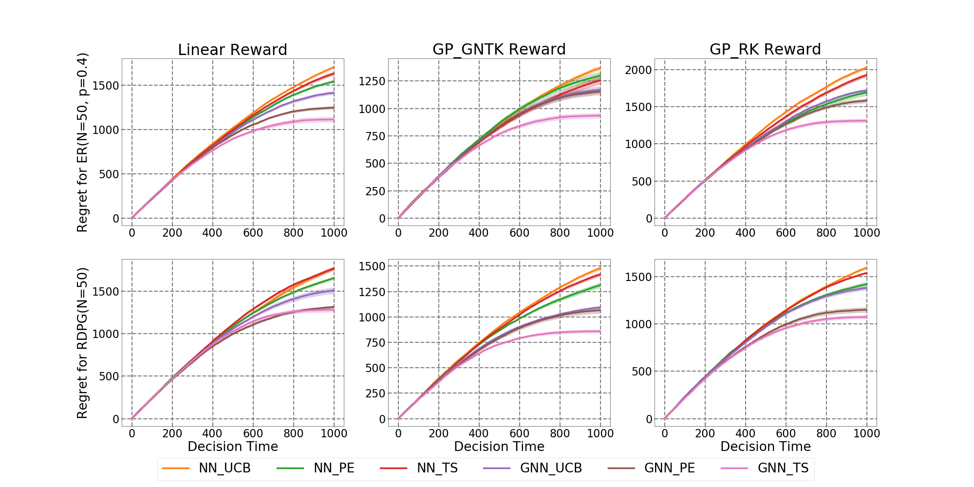
Figure 1: Regret over horizon $T=1000$ for Erdös–Rényi random graphs with $p=0.4$ and $N=50$ in the first row and random dot product graphs with $N=50$. Three columns are three types of reward function generation: linear model, Gaussian process with GNTK, Gaussian process with representation kernel. GNN-TS is competitive and robust to different environment settings.

6 Experiments

We create synthetic graph data and generate the rewards through three different mechanisms. For the graph structures, we use random graph models including Erdös–Rényi and random dot product graph models. The features are generated i.i.d. from the ${\mathcal{N}}(0,1)$. The noisy reward is assumed to have $\sigma_{\varepsilon}=0.01$. Our experiments investigate GNN-UCB, GNN-PE, NN-UCB, NN-PE, and NN-TS as baselines from Kassraie et al. [2022]. All performance curves in our empirical studies show an average of over $10$ repetitions with a standard deviation of the corresponding bandit algorithm with horizon $T=1000$. We assume the graph domain is fully observable, ${\mathcal{G}}_{t}={\mathcal{G}}$ for all $t\in[T]$. Below is a brief overview of the simulation elements. For more details, see Appendix D.

Random Graph. We use two types of random graphs including Erdös–Rényi (ER) random graphs and random dot product graphs (RDPG). ER graphs are generated with edge probability $p$ and number of nodes $N$. RDPGs are generated by modeling the expected edge probabilities as the function of the inner product of features. In the first row of Figure 1, the graphs in ${\mathcal{G}}$ are from the ER model with $p=0.4$ and in the second row from an RDPG, both of size $N=50$.

Reward Function. To generate the rewards, we use models of three different types: linear model, Gaussian Process (GP) with GNTK, Gaussian process with the representation kernel. For the linear model, we have $\mu(G)=\langle{\boldsymbol{\theta}}^{*},\bar{{\boldsymbol{h}}}^{G}\rangle$ with true parameter ${\boldsymbol{\theta}}^{*}\sim\mathcal{N}(0,{\boldsymbol{I}}_{d})$ and $\bar{{\boldsymbol{h}}}^{G}=\sum_{i=1}^{N}{\boldsymbol{h}}^{G}_{i}/N$. For the GP with GNTK, we fit a GP regression model with empirical GNTK matrix $\hat{\boldsymbol{K}}\in\mathbb{R}^{|{\mathcal{G}}|\times|{\mathcal{G}}|}$ as the covariance matrix of the prior, trained on $\{(G,y_{G})\}_{G\in{\mathcal{G}}}$ where $\{y_{G}\}_{G\in{\mathcal{G}}}$ are i.i.d. from ${\mathcal{N}}(0,1)$. For the GP with the representation kernel, we trained a GNN for a graph property prediction task and used the mean pooling over all the nodes of the last layer representations as the graph representation, denoted as $\bar{\boldsymbol{h}}^{G}_{\text{rep}}$. We then define the representation kernel as $k_{\text{rep}}(G,G^{\prime}):=\langle\bar{\boldsymbol{h}}^{G}_{\text{rep}},\bar{\boldsymbol{h}}^{G^{\prime}}_{\text{rep}}\rangle$ and draw $\mu(\cdot)$ from a zero-mean GP with this covariance function (over $\mathcal{G}$).

Algorithms. We investigate two baselines GNN-UCB and GNN-PE along with our proposed GNN-TS. GNN-PE is the proposed state-of-the-art algorithm that selects the graph with the highest uncertainty and eliminates the graph candidates by the upper confidence bounds. All the algorithms in our work use the loss function (6) which is different from previous work. All gradients used for our experiments are ${\boldsymbol{\textnormal{{g}}}}(G;{\boldsymbol{\theta}}_{t})$, not ${\boldsymbol{\textnormal{{g}}}}(G;{\boldsymbol{\theta}}_{0})$, unless otherwise specified. In addition, in order to show the benefit of considering the graph structure, we include NN-UCB, NN-TS, and NN-PE as our baselines. For these NN-based algorithms, we ignore the adjacency matrix of a graph (setting ${\boldsymbol{A}}={\boldsymbol{I}}_{N}$), and pass through the model in (1) and (2) with ${\boldsymbol{h}}^{G}_{i}={\boldsymbol{X}}_{i*}$. The MLPs in our experiments have $L=2$ layers and width $m=512$. We use SGD as the optimizer, with mini-batch size $5$, and train for $30$ epochs. For the tuning of the hyperparameters $(\eta,\lambda)$ and other algorithmic setup, see Appendix D. The matrix inversion in the algorithms is approximated by diagonal inversion across all policy algorithms.

Regret Experiments. In Figure 1, we show the performance of all the algorithms for the six possible environments: ER or RDPG model coupled with either of the three reward models. We set the size of the graph domain to $|{\mathcal{G}}|=100$ in Figure 1 and we experiment across different $|{\mathcal{G}}|$ in Appendix D. Figure 1 demonstrates that GNN-TS consistently outperforms the baseline algorithms and is robust to all types of random graph models and reward function generations in our experiment. In addition, GNN-based algorithms are clearly better than NN-based algorithms in graph action bandit settings.

Appendix A Proof for Lemmas in Regret Analysis

A.1 Notations

In the following parts, we further define the some notations to represent the linear and kernelized models:

$${\boldsymbol{G}}_{t} =[{\boldsymbol{\textnormal{{g}}}}(G_{1};{\boldsymbol{\theta}}_{0}),...,{\boldsymbol{\textnormal{{g}}}}(G_{t};{\boldsymbol{\theta}}_{t-1}))]\in\mathbb{R}^{p\times t}$$ (23)

$$\bar{{\boldsymbol{G}}}_{t} =[{\boldsymbol{\textnormal{{g}}}}(G_{1};{\boldsymbol{\theta}}_{0}),...,{\boldsymbol{\textnormal{{g}}}}(G_{t};{\boldsymbol{\theta}}_{0})]\in\mathbb{R}^{p\times t}$$

$${\boldsymbol{\mu}}_{t} =[\mu(G_{1}),...,\mu(G_{t})]^{\top}\in\mathbb{R}^{t\times 1}$$

$${\boldsymbol{y}}_{t} =[y_{1},...,y_{t}]^{\top}\in\mathbb{R}^{t\times 1}$$

$${\boldsymbol{\epsilon}}_{t} =[\varepsilon_{1},...,\varepsilon_{t}]^{\top}\in\mathbb{R}^{t\times 1}.$$

Then we define the uncertainty estimate with initial gradient ${\boldsymbol{\theta}}_{0}$:

$$\bar{\sigma}_{t}^{2}(G)=\frac{1}{m}\|{\boldsymbol{\textnormal{{g}}}}(G;{\boldsymbol{\theta}}_{0})\|_{\bar{{\boldsymbol{U}}}_{t-1}^{-1}}^{2}\quad\text{and}\quad\bar{{\boldsymbol{U}}}_{t}=\lambda{\boldsymbol{I}}_{p}+\sum_{i=1}^{t}{\boldsymbol{\textnormal{{g}}}}(G_{i};{\boldsymbol{\theta}}_{0}){\boldsymbol{\textnormal{{g}}}}(G_{i};{\boldsymbol{\theta}}_{0})^{\top}/m.$$ (24)

A.2 Proof of Lemma 5.1

Let us write

$$\widetilde{{\boldsymbol{\theta}}}_{t-1}:=\bar{{\boldsymbol{U}}}_{t-1}^{-1}\bar{{\boldsymbol{G}}}_{t-1}{\boldsymbol{y}}_{t-1}/m$$

for the ridge regression solution. We will need the following auxiliary lemmas:

Lemma A.1 (Taylor Approximation of a GNN).

Suppose learning rate $\eta\leq(\tilde{C}mL+m\lambda)^{-1}$ for some constant $\tilde{C}$, then for any fixed $t\in[T]$ and $G\in{\mathcal{G}}$, with probability at least $1-\delta$

$$|f_{\operatorname{GNN}}(G;{\boldsymbol{\theta}}_{t}^{(J)})-f_{\operatorname{GNN}}(G;{\boldsymbol{\theta}}_{0})-\langle{\boldsymbol{\textnormal{{g}}}}(G;{\boldsymbol{\theta}}_{0}),{\boldsymbol{\theta}}_{t}^{(J)}-{\boldsymbol{\theta}}_{0}\rangle|\leq CL^{3}\Bigl{(}\frac{R^{2}+\sigma_{\varepsilon}^{2}}{m\lambda}\Bigr{)}^{2/3}\sqrt{m\log(m)}$$ (25)

where $C$ is some constant independent of $m$ and $t$.

Lemma A.2.

Suppose $m\geq poly(R,\sigma_{\varepsilon},L,\lambda^{-1},|{\mathcal{G}}|,\rho_{min}^{-1},\log(LN|{\mathcal{G}}|/\delta))$ given a fixed $\delta\in(0,1)$ and learning rate $\eta\leq(\tilde{C}mL+m\lambda)^{-1}$ for some constant $\tilde{C}$. For $G\in{\mathcal{G}}_{t}$ and $t>1$, with probability at lease $1-\delta$,

$$|\langle{\boldsymbol{\textnormal{{g}}}}(G;{\boldsymbol{\theta}}_{0}),{\boldsymbol{\theta}}_{t-1}-{\boldsymbol{\theta}}_{0}-\widetilde{{\boldsymbol{\theta}}}_{t-1}\rangle|\leq C\bar{\sigma}_{t}(G)$$ (26)

where $C=(C_{1}(2-\eta m\lambda)^{J}+C_{2})\sqrt{\frac{\sigma_{\varepsilon}^{2}+R^{2}}{\lambda}(1+\frac{3\rho_{\max}}{2\lambda})}$ with $C_{1}={\mathcal{O}}(1)$ and $C_{2}={\mathcal{O}}(\lambda^{1/3})$.

Lemma A.3.

Fix $\delta\in(0,1)$ and let $m=\Omega(L^{10}T^{4}|{\mathcal{G}}|^{6}\rho_{min}^{-4}\log(LN^{2}|{\mathcal{G}}|^{2}/\delta)).$ Then, there exists ${\boldsymbol{\theta}}^{*}\in\mathbb{R}^{p}$ with $\sqrt{m}\|{\boldsymbol{\theta}}^{*}\|_{2}\leq\sqrt{2}R$ such that with probability at least $1-\delta$,

$$\mu(G) =\langle{\boldsymbol{\textnormal{{g}}}}(G;{\boldsymbol{\theta}}_{0}),{\boldsymbol{\theta}}^{*}\rangle,\quad\text{for all $G\in\mathcal{G}$}$$ (27)

$$\log\det(\lambda^{-1}\bar{{\boldsymbol{U}}}_{t}) \leq\log\det({\boldsymbol{I}}_{|{\mathcal{G}}|}+\lambda^{-1}t{\boldsymbol{K}})+1.$$

Lemma A.4.

With probability at least $1-\delta$, we have

$$|\bar{\sigma}_{t}(G)-\sigma_{t}(G)|\leq Ct\lambda^{-1/6}L^{9/2}(R^{2}+\sigma_{\varepsilon}^{2})^{1/6}m^{-1/6}\sqrt{\log(m)}.$$ (28)

We choose an arbitrary small $\delta\in(0,1)$ and set $\delta_{i}=\delta/(5T)$ for $i=1,\dots,5$. For all $\forall G\in{\mathcal{G}}_{t}$, we have

$$|f_{\operatorname{GNN}}(G;{\boldsymbol{\theta}}_{t-1})-\mu(G)|\leq\underbrace{|f_{\operatorname{GNN}}(G;{\boldsymbol{\theta}}_{t-1})-\langle{\boldsymbol{\textnormal{{g}}}}(G;{\boldsymbol{\theta}}_{0}),\widetilde{{\boldsymbol{\theta}}}_{t-1}\rangle|}_{:=I_{1}}+\underbrace{|\mu(G)-\langle{\boldsymbol{\textnormal{{g}}}}(G;{\boldsymbol{\theta}}_{0}),\widetilde{{\boldsymbol{\theta}}}_{t-1}\rangle|}_{:=I_{2}}.$$ (29)

We then turn to bounding $I_{1}$ and $I_{2}$. Throughout the proof, let

$$\gamma_{m}:=m^{-1/6}\sqrt{\log m}$$ (30)

Bounding $I_{1}$: By Lemma A.1 and Lemma A.2, with probability at least $1-\delta_{1}-\delta_{2}$,

$$I_{1} =|f_{\operatorname{GNN}}(G;{\boldsymbol{\theta}}_{t-1})-\langle{\boldsymbol{\textnormal{{g}}}}(G;{\boldsymbol{\theta}}_{0}),\widetilde{{\boldsymbol{\theta}}}_{t-1}\rangle|$$ (31)

$$\leq|f_{\operatorname{GNN}}(G;{\boldsymbol{\theta}}_{t-1})-\langle{\boldsymbol{\textnormal{{g}}}}(G;{\boldsymbol{\theta}}_{0}),{\boldsymbol{\theta}}_{t-1}-{\boldsymbol{\theta}}_{0}\rangle|+|\langle{\boldsymbol{\textnormal{{g}}}}(G;{\boldsymbol{\theta}}_{0}),{\boldsymbol{\theta}}_{t-1}-{\boldsymbol{\theta}}_{0}-\widetilde{{\boldsymbol{\theta}}}_{t-1}\rangle|$$

$$\leq C_{0}L^{3}\gamma_{m}+\tilde{C}_{2}\,\bar{\sigma}_{t}(G).$$

where $C_{0}:=\tilde{C}_{1}\Bigl{(}\frac{R^{2}+\sigma_{\varepsilon}^{2}}{\lambda}\Bigr{)}^{2/3}$ and $\tilde{C}_{2}:=(\bar{C}_{1}(2-\eta m\lambda)^{J}+\bar{C}_{2}\lambda^{1/3})\sqrt{\frac{\sigma_{\varepsilon}^{2}+R^{2}}{\lambda}(1+\frac{3\rho_{\max}}{2\lambda})}$ for some constant $\bar{C}_{1}$, $\bar{C}_{2}$. For $\lambda\gtrsim(\sigma_{\varepsilon}^{2}+R^{2})^{3}+\rho_{\max}$, we have $C_{0},\tilde{C}_{2}\lesssim 1$ subject to the constraint in $\eta$ in Lemma A.2. Thus, we obtain

$$I_{1}\lesssim L^{3}\gamma_{m}+\bar{\sigma}_{t}(G).$$

Bounding $I_{2}$: By Lemma B.5, with at least probability $1-\delta_{3}$, for all $G\in\mathcal{G}$, we have

$$I_{2}=|\langle{\boldsymbol{\textnormal{{g}}}}(G;{\boldsymbol{\theta}}_{0}),{\boldsymbol{\theta}}^{*}-\widetilde{{\boldsymbol{\theta}}}_{t-1}\rangle|.$$

Recall that ${\boldsymbol{y}}_{t-1}={\boldsymbol{\mu}}_{t-1}+{\boldsymbol{\epsilon}}_{t-1}$ and by Lemma A.3, we have ${\boldsymbol{\mu}}_{t-1}=\bar{{\boldsymbol{G}}}_{t-1}^{\top}{\boldsymbol{\theta}}^{*}$. Then,

$$\widetilde{{\boldsymbol{\theta}}}_{t-1}=\bar{{\boldsymbol{U}}}_{t-1}^{-1}\bar{{\boldsymbol{G}}}_{t-1}\bar{{\boldsymbol{G}}}_{t-1}^{\top}{\boldsymbol{\theta}}^{*}/m+\bar{{\boldsymbol{U}}}_{t-1}^{-1}\bar{{\boldsymbol{G}}}_{t-1}{\boldsymbol{\epsilon}}_{t-1}/m$$

We have $\bar{\boldsymbol{U}}_{t}=\lambda{\boldsymbol{I}}_{p}+\bar{\boldsymbol{G}}_{t}\bar{\boldsymbol{G}}_{t}^{\top}/m$. Hence, $\bar{\boldsymbol{U}}_{t}^{-1}\bar{\boldsymbol{G}}_{t}\bar{\boldsymbol{G}}_{t}^{\top}/m=\bar{\boldsymbol{U}}_{t}^{-1}(\bar{\boldsymbol{U}}_{t}-\lambda{\boldsymbol{I}}_{p})={\boldsymbol{I}}_{p}-\lambda\bar{\boldsymbol{U}}_{t}^{-1}$. This gives

$$\widetilde{{\boldsymbol{\theta}}}_{t-1}={\boldsymbol{\theta}}^{*}-\lambda\bar{\boldsymbol{U}}_{t-1}^{-1}{\boldsymbol{\theta}}^{*}+\frac{1}{\sqrt{m}}\,\bar{{\boldsymbol{U}}}_{t-1}^{-1}\boldsymbol{S}_{t-1}$$

where we have defined $\boldsymbol{S}_{t-1}:=\frac{1}{\sqrt{m}}\bar{{\boldsymbol{G}}}_{t-1}{\boldsymbol{\epsilon}}_{t-1}$. Thus, we have

$$I_{2}\leq\lambda|\langle{\boldsymbol{\textnormal{{g}}}}(G;{\boldsymbol{\theta}}_{0}),\bar{\boldsymbol{U}}_{t}^{-1}{\boldsymbol{\theta}}^{*}\rangle|+\frac{1}{\sqrt{m}}|\langle{\boldsymbol{\textnormal{{g}}}}(G;{\boldsymbol{\theta}}_{0}),\bar{\boldsymbol{U}}_{t-1}^{-1}\boldsymbol{S}_{t-1}\rangle|$$ (32)

Recall that $\sqrt{m}\bar{\sigma}_{t}(G)=\|{\boldsymbol{\textnormal{{g}}}}(G;{\boldsymbol{\theta}}_{0})\|_{\bar{{\boldsymbol{U}}}_{t-1}^{-1}}$. Since $\bar{{\boldsymbol{U}}}_{t-1}^{-1}\preccurlyeq\frac{1}{\lambda}{\boldsymbol{I}}_{p}$, for any vector ${\boldsymbol{v}}$, we have $\|{\boldsymbol{v}}\|_{\bar{{\boldsymbol{U}}}_{t-1}^{-1}}\leq\frac{1}{\sqrt{\lambda}}\|{\boldsymbol{v}}\|$. Then, for the first term in (32), we have

$$\lambda|{\boldsymbol{\textnormal{{g}}}}(G;{\boldsymbol{\theta}}_{0})^{\top}\bar{{\boldsymbol{U}}}_{t-1}^{-1}{\boldsymbol{\theta}}^{*}| \leq\lambda\|{\boldsymbol{\textnormal{{g}}}}(G;{\boldsymbol{\theta}}_{0})\|_{\bar{{\boldsymbol{U}}}_{t-1}^{-1}}\cdot\|{\boldsymbol{\theta}}^{*}\|_{\bar{{\boldsymbol{U}}}_{t-1}^{-1}}$$

$$\leq\sqrt{m}\bar{\sigma}_{t}(G)\cdot\sqrt{\lambda}\|{\boldsymbol{\theta}}^{*}\|_{2}\leq\bar{\sigma}_{t}(G)\sqrt{2\lambda}R$$

where we have used Cauchy-Schwarz inequality for $\langle\cdot,\cdot\rangle_{{\boldsymbol{U}}_{t-1}^{-1}}$ and Lemma A.3. For the second term in (32), we have

$$\frac{1}{\sqrt{m}}|{\boldsymbol{\textnormal{{g}}}}(G;{\boldsymbol{\theta}}_{0})^{\top}\bar{{\boldsymbol{U}}}_{t-1}^{-1}\boldsymbol{S}_{t-1}| \leq\frac{1}{\sqrt{m}}\|{\boldsymbol{\textnormal{{g}}}}(G;{\boldsymbol{\theta}}_{0})\|_{\bar{{\boldsymbol{U}}}_{t-1}^{-1}}\|\boldsymbol{S}_{t-1}\|_{\bar{{\boldsymbol{U}}}_{t-1}^{-1}}=\bar{\sigma}_{t}(G)\cdot\|\boldsymbol{S}_{t-1}\|_{\bar{{\boldsymbol{U}}}_{t-1}^{-1}}$$

By Theorem 20.4 of Lattimore and Szepesvári [2020], with probability at least $1-\delta_{4}$, we have

$$\frac{1}{\sigma_{\varepsilon}^{2}}\|\boldsymbol{S}_{t}\|_{\bar{{\boldsymbol{U}}}_{t}^{-1}}^{2}\leq 2\log(1/\delta_{4})+\log\deg(\lambda^{-1}\bar{\boldsymbol{U}}_{t}),\quad\text{for all}\;t\in\mathbb{N}.$$

By Lemma A.3, with high probability,

$$\log\det(\lambda^{-1}\bar{\boldsymbol{U}}_{t})\leq\log\det({\boldsymbol{I}}_{|\mathcal{G}|}+T{\boldsymbol{K}}/\lambda)+1\leq 2\tilde{d}\log(1+T\rho_{\max}/\lambda).$$ (33)

Using $\lambda\gtrsim\rho_{\max}$, we have $\log\det(\lambda^{-1}\bar{\boldsymbol{U}}_{t})\lesssim\tilde{d}\log(T)+1\lesssim\tilde{d}\log(T)$. We also have $\log(1/\delta_{4})=\log(5T)\lesssim\log(T)\lesssim\tilde{d}\log(T)$.

Putting the pieces together, we have

$$\frac{1}{\sqrt{m}}|{\boldsymbol{\textnormal{{g}}}}(G;{\boldsymbol{\theta}}_{0})^{\top}\bar{{\boldsymbol{U}}}_{t-1}^{-1}\boldsymbol{S}_{t-1}|\lesssim\sigma_{\varepsilon}\sqrt{\tilde{d}\log T}\cdot\bar{\sigma}_{t}(G).$$

Combining with the first term, we obtain

$$I_{2}\lesssim\bigl{(}\sigma_{\varepsilon}\sqrt{\tilde{d}\log T}+\sqrt{\lambda}R\bigr{)}\bar{\sigma}_{t}(G).$$

Combining with the bound on $I_{1}$, we have

$$|f_{\operatorname{GNN}}(G;{\boldsymbol{\theta}}_{t-1})-\mu(G)| \lesssim L^{3}\gamma_{m}+\bigl{(}1+\sigma_{\varepsilon}\sqrt{\tilde{d}\log T}+\sqrt{\lambda}R\bigr{)}\,\bar{\sigma}_{t}(G)$$

$$=:L^{3}\gamma_{m}+\alpha\,\bar{\sigma}_{t}(G)$$

where we have set $\alpha:=1+\sigma_{\varepsilon}\sqrt{\tilde{d}\log T}+\sqrt{\lambda}R$ for simplificty.

By Lemma A.4, with probability at least $1-\delta_{5}$,

$$\bar{\sigma}_{t}(G)-\sigma_{t}(G)\leq CtL^{9/2}\Bigl{(}\frac{R^{2}+\sigma_{\varepsilon}^{2}}{\lambda}\Bigr{)}^{1/6}\gamma_{m}\lesssim t\cdot L^{9/2}\gamma_{m}$$

using the assumption $\lambda\gtrsim R^{2}+\sigma_{\varepsilon}^{2}$. We obtain

$$|f_{\operatorname{GNN}}(G;{\boldsymbol{\theta}}_{t-1})-\mu(G)| \lesssim L^{3}\gamma_{m}+t\cdot\alpha L^{9/2}\gamma_{m}+\alpha\sigma_{t}(G)$$

$$\leq 2t\cdot\alpha L^{9/2}\gamma_{m}+\alpha\sigma_{t}(G)$$

since $t\geq 1$ and $\alpha\geq 1$. Taking $\nu\geq\alpha$ finishes the proof.

A.3 Proof of Lemma 5.2

Proof of Lemma 5.2.

Conditioned on $\mathcal{F}_{t}$, we have

$$\widehat{r}_{t}(G)\,|\,\mathcal{F}_{t}\sim{\mathcal{N}}(f_{\operatorname{GNN}}(G;{\boldsymbol{\theta}}_{t-1}),\nu^{2}\sigma_{t}^{2}(G)).$$ (34)

Using standard Gaussian tail bound, followed by a union bound gives

$$\mathbb{P}_{t}(|\widehat{r}_{t}(G)-f_{\operatorname{GNN}}(G;{\boldsymbol{\theta}}_{t-1})|\geq\nu\sigma_{t}(G)\cdot u)\leq|\mathcal{G}_{t}|e^{-u^{2}/2}$$ (35)

which shows the first assertion by letting $u=\sqrt{2\log(t^{2}|{\mathcal{G}}_{t}|)}$.

For the second assertion, it is enough to note that $\mathbb{P}(Z\geq 1)\geq(4e\sqrt{\pi})^{-1}$ for $Z\sim{\mathcal{N}}(0,1)$. ∎

A.4 Proof of Lemma 5.3

Proof of Lemma 5.3.

Our proof is inspired from the proof in Wu et al. [2022]. Recall that $c_{t}^{\mu}(G)=\nu\sigma_{t}(G)+\varepsilon(t,m)$ and $c_{t}^{\sigma}(G):=\nu\sigma_{t}(G)\sqrt{2\log(t^{2}|{\mathcal{G}}_{t}|)}$ and

$${\mathcal{E}}_{t}^{\mu} =\{\forall G\in{\mathcal{G}}_{t},|f_{\operatorname{GNN}}(G;{\boldsymbol{\theta}}_{t-1})-\mu(G)|\leq c_{t}^{\mu}(G)\}$$ (36)

$${\mathcal{E}}_{t}^{\sigma} =\{\forall G\in{\mathcal{G}}_{t},|\widehat{r}_{t}(G)-f_{\operatorname{GNN}}(G;{\boldsymbol{\theta}}_{t-1})|\leq c_{t}^{\sigma}(G)\}$$

Let $\gamma_{t}(G)=c_{t}^{\mu}(G)+c_{t}^{\sigma}(G)$ and $c_{t}(G)=\gamma_{t}(G)+\varepsilon(t,m)$. Then, on $\mathcal{E}_{t}^{\mu}\cap\mathcal{E}_{t}^{\sigma}$, by triangle inequality,

$$|\widehat{r}_{t}(G)-\mu(G)|\leq\gamma_{t}(G).$$ (37)

We also recall that $\mathcal{E}^{a}_{t}:=\{\widehat{r}_{t}(G^{*}_{t})-f_{\operatorname{GNN}}(G^{*}_{t};{\boldsymbol{\theta}}_{t-1})>\nu\sigma_{t}(G^{*}_{t})\}$. Then, on $\mathcal{E}_{t}^{\mu}\cap\mathcal{E}_{t}^{a}$, we have

$$\widehat{r}_{t}(G^{*}_{t}) >f_{\operatorname{GNN}}(G^{*}_{t};{\boldsymbol{\theta}}_{t-1})+\nu\sigma_{t}(G^{*}_{t})$$

$$\geq\mu(G^{*}_{t})-c_{t}^{\mu}(G^{*}_{t})+\nu\sigma_{t}(G^{*}_{t})$$

$$=\mu(G^{*}_{t})-\varepsilon(t,m)$$ (38)

Recall that $\Delta_{t}:=\mu(G^{*}_{t})-\mu(G_{t})$ for convenience. Consider the set of unsaturated actions

$$\mathcal{U}_{t}=\bigr{\{}G\in\mathcal{G}_{t}:\;\mu(G^{*}_{t})<\mu(G)+c_{t}(G)\bigl{\}}$$

and let $\bar{G}_{t}$ be the least uncertain unsaturated action at time $t$:

$$\bar{G}_{t}:=\operatorname*{argmin}_{G\in\mathcal{U}_{t}}c_{t}(G).$$ (39)

By $\bar{G}_{t}\in\mathcal{U}_{t}$, we have $\Delta_{t}\leq c_{t}(\bar{G}_{t})+\mu(\bar{G}_{t})-\mu(G_{t}).$ Applying (37), twice, on $\mathcal{E}_{t}^{\mu}\cap\mathcal{E}_{t}^{\sigma}$, we have

$$\Delta_{t} \leq c_{t}(\bar{G}_{t})+\gamma_{t}(\bar{G}_{t})+\gamma_{t}(G_{t})+\widehat{r}_{t}(\bar{G}_{t})-\widehat{r}_{t}(G_{t})$$

$$\leq\ c_{t}(\bar{G})+\gamma_{t}(\bar{G}_{t})+\gamma_{t}(G_{t})$$

for all $G\in\mathcal{G}_{t}$ where the second inequality follows since $G_{t}$ maximizes $\widehat{r}_{t}(\cdot)$ over $\mathcal{G}_{t}$, by design.

Recall that $\mathbb{E}_{t}[\cdot]=\mathbb{E}[\cdot\,|\,\mathcal{F}_{t}]$, where $\mathcal{F}_{t}$ is the history up to (but not including) time $t$. Given $\mathcal{F}_{t}$, the event $\mathcal{E}_{t}^{\mu}$ is deterministic while $\mathcal{E}_{t}^{\sigma}$ is only random due to the independent randomness in the sampling step (4). Next, we have

$$\mathbb{E}_{t}[\Delta_{t}\mathbb{I}_{\mathcal{E}_{t}^{\mu}}] =\mathbb{I}_{\mathcal{E}_{t}^{\mu}}\cdot\mathbb{E}_{t}[\Delta_{t}]$$

$$=\mathbb{I}_{\mathcal{E}_{t}^{\mu}}\cdot\bigl{(}\mathbb{E}_{t}[\Delta_{t}\mathbb{I}_{\mathcal{E}_{t}^{\sigma}}]+\mathbb{E}_{t}[\Delta_{t}\mathbb{I}_{\bar{\mathcal{E}}_{t}^{\sigma}}]\bigr{)}$$

$$\leq\mathbb{I}_{\mathcal{E}_{t}^{\mu}}\cdot\bigl{(}\mathbb{E}_{t}[\Delta_{t}\mathbb{I}_{\mathcal{E}_{t}^{\sigma}}]+B\,\mathbb{P}_{t}(\bar{\mathcal{E}}_{t}^{\sigma})\bigr{)}$$ (40)

using the boundedness Assumption 2. Here, we are using the fact that $\mathcal{E}_{t}^{\mu}$ is measurable w.r.t. $\mathcal{F}_{t}$, hence it is deterministic conditioned on $\mathcal{F}_{t}$. Due to factor $\mathbb{I}_{\mathcal{E}_{t}^{\mu}}$ in the above, the bound is trivial when $\mathcal{E}_{t}^{\mu}$ fails, so for the rest of the proof we assume that $\mathcal{E}_{t}^{\mu}$ holds (conditioned on $\mathcal{F}_{t}$).

We have

$$\mathbb{E}_{t}[\Delta_{t}\mathbb{I}_{\mathcal{E}_{t}^{\sigma}}] \leq c_{t}(\bar{G}_{t})+\gamma_{t}(\bar{G}_{t})+\mathbb{E}_{t}[\gamma_{t}(G_{t})\mathbb{I}_{\mathcal{E}_{t}^{\sigma}}]$$

$$\leq 2c_{t}(\bar{G}_{t})-\varepsilon(t,m)+\mathbb{E}_{t}[\gamma_{t}(G_{t})]$$

where we have used the definition of $c_{t}(\cdot)$ and dropped the indicator $\mathbb{I}_{\mathcal{E}_{t}^{\sigma}}$ to get a further upper bound. It remains to bound $c_{t}(\bar{G}_{t})$ in terms of $\gamma_{t}(G_{t})$.

Since $\bar{G}_{t}$ is the least uncertain unsaturated action, we have

$$c_{t}(\bar{G}_{t})\mathbb{I}\{G_{t}\in\mathcal{U}_{t}\}\leq c_{t}(G_{t}).$$

Multiplying both sides by $\mathbb{I}_{\mathcal{E}_{\sigma}^{t}}$, taking $\mathbb{E}_{t}[\cdot]$, and rearranging

$$c_{t}(\bar{G}_{t})\leq\frac{\mathbb{E}_{t}[c_{t}(G_{t})\mathbb{I}_{\mathcal{E}_{\sigma}^{t}}]}{\mathbb{P}_{t}(\{G_{t}\in\mathcal{U}_{t}\}\cap\mathcal{E}_{t}^{\sigma})}\leq\frac{\mathbb{E}_{t}[\gamma_{t}(G_{t})]}{\mathbb{P}_{t}(\{G_{t}\in\mathcal{U}_{t}\}\cap\mathcal{E}_{t}^{\sigma})}.$$

It remains to bound the denominator.

Recall that $G_{t}$ maximizes $\widehat{r}_{t}(\cdot)$ over the entire $\mathcal{G}_{t}$. Thus, if

$$\widehat{r}_{t}(G_{t}^{*})>\max_{G\,\in\,\bar{\mathcal{U}}_{t}}\widehat{r}_{t}(G)$$ (41)

then $G_{t}$ cannot belong to $\bar{\mathcal{U}}_{t}$, hence $G_{t}\in\mathcal{U}_{t}$. On $\mathcal{E}_{t}^{\mu}\cap\mathcal{E}_{t}^{\sigma}$, for any $G\in\bar{\mathcal{U}}_{t}$, we have

$$\widehat{r}_{t}(G)\leq\mu(G)+\gamma_{t}(G) \leq\mu(G^{*}_{t})-c_{t}(G)+\gamma_{t}(G)$$

$$\leq\mu(G^{*}_{t})-\varepsilon(t,m)$$

where the second inequality is by the definition of $\bar{\mathcal{U}}_{t}$. Then for (41) to hold on $\mathcal{E}_{t}^{\mu}\cap\mathcal{E}_{t}^{\sigma}$, it is enough to have $\widehat{r}_{t}(G_{t}^{*})>\mu(G_{t}^{*})-\varepsilon(t,m)$. But this holds on $\mathcal{E}_{t}^{\mu}\cap\mathcal{E}_{t}^{a}$ by (38). That is,

$$\mathcal{E}_{t}^{a}\cap\mathcal{E}_{t}^{\mu}\cap\mathcal{E}_{t}^{\sigma} \subset\{\widehat{r}_{t}(G_{t}^{*})>\mu(G_{t}^{*})-\varepsilon(t,m)\}\cap\mathcal{E}_{t}^{\mu}\cap\mathcal{E}_{t}^{\sigma}$$

$$\subset\{\widehat{r}_{t}(G_{t}^{*})>\max_{G\,\in\,\bar{\mathcal{U}}_{t}}\widehat{r}_{t}(G)\}\cap\mathcal{E}_{t}^{\mu}\cap\mathcal{E}_{t}^{\sigma}$$

$$\subset\{G_{t}\in\mathcal{U}_{t}\}\cap\mathcal{E}_{t}^{\mu}\cap\mathcal{E}_{t}^{\sigma}.$$

Assuming as before that $\mathcal{E}_{t}^{\mu}$ holds, we have

$$\mathbb{P}_{t}(\mathcal{E}_{t}^{a}\cap\mathcal{E}_{t}^{\sigma})\leq\mathbb{P}_{t}(\{G_{t}\in\mathcal{U}_{t}\}\cap\mathcal{E}_{t}^{\sigma}).$$ (42)

We have $\mathbb{P}_{t}(\mathcal{E}_{t}^{a}\cap\mathcal{E}_{t}^{\sigma})\geq\mathbb{P}_{t}(\mathcal{E}_{t}^{a})-\mathbb{P}_{t}(\bar{\mathcal{E}}_{t}^{\sigma})$. Putting the pieces together

$$c_{t}(\bar{G}_{t})\leq\frac{\mathbb{E}_{t}[\gamma_{t}(G_{t})]}{\mathbb{P}_{t}(\mathcal{E}_{t}^{a})-\mathbb{P}_{t}(\bar{\mathcal{E}}_{t}^{\sigma})}$$

and we obtain

$$\mathbb{E}_{t}[\Delta_{t}\mathbb{I}_{\mathcal{E}_{t}^{\sigma}}]\leq\Bigl{(}\frac{2}{\mathbb{P}_{t}(\mathcal{E}_{t}^{a})-\mathbb{P}_{t}(\bar{\mathcal{E}}_{t}^{\sigma})}+1\Bigr{)}\mathbb{E}_{t}[\gamma_{t}(G_{t})]-\varepsilon(t,m)$$

Combining with (40) the result follows. ∎

A.5 Proof of Lemma 5.4

Proof of Lemma 5.4.

For simplicity, we define

$${\boldsymbol{\textnormal{{g}}}}_{t}:=\frac{1}{\sqrt{m}}{\boldsymbol{\textnormal{{g}}}}(G_{t};{\boldsymbol{\theta}}_{t-1}),\quad\bar{{\boldsymbol{\textnormal{{g}}}}}_{t}:=\frac{1}{\sqrt{m}}{\boldsymbol{\textnormal{{g}}}}(G_{t};{\boldsymbol{\theta}}_{0}).$$ (43)

Then, recall that

$$\sigma_{t}^{2}(G_{t})=\|{\boldsymbol{\textnormal{{g}}}}_{t}\|_{{\boldsymbol{U}}_{t-1}^{-1}}^{2},\quad{\boldsymbol{U}}_{t-1}=\lambda{\boldsymbol{I}}_{p}+\sum_{i=1}^{t-1}{\boldsymbol{\textnormal{{g}}}}_{t}{\boldsymbol{\textnormal{{g}}}}_{t}^{\top}.$$

Note that ${\boldsymbol{U}}_{t}={\boldsymbol{U}}_{t-1}+{\boldsymbol{\textnormal{{g}}}}_{t}{\boldsymbol{\textnormal{{g}}}}_{t}^{\top}$.

Then we introduce following Lemmas:

Lemma A.5 (Elliptical Potential).

Assume that ${\boldsymbol{U}}_{t}={\boldsymbol{U}}_{t-1}+{\boldsymbol{\textnormal{{g}}}}_{t}{\boldsymbol{\textnormal{{g}}}}_{t}^{\top}$ for all $t\in[T]$. Then,

$$\sum_{t=1}^{T}\min\{1,\|{\boldsymbol{\textnormal{{g}}}}_{t}\|_{{\boldsymbol{U}}_{t-1}^{-1}}^{2}\}\leq 2\log\Big{(}\frac{\det{\boldsymbol{U}}_{T}}{\det{\boldsymbol{U}}_{0}}\Big{)}.$$ (44)

Lemma A.6.

Let ${\boldsymbol{A}}=[{\boldsymbol{a}}_{1}\;{\boldsymbol{a}}_{2}\;\cdots\;{\boldsymbol{a}}_{n}]$ and $\boldsymbol{\bar{A}}=[\bar{{\boldsymbol{a}}}_{1}\;\bar{{\boldsymbol{a}}}_{2}\;\cdots\;\bar{{\boldsymbol{a}}}_{n}]$ be $p\times n$ matrices, with columns $\{{\boldsymbol{a}}_{i}\}$ and $\{\bar{{\boldsymbol{a}}}_{i}\}$, respectively. Assume that for $\varepsilon\leq C$, we have

$$\|{\boldsymbol{a}}_{i}-\bar{{\boldsymbol{a}}}_{i}\|\leq\varepsilon,\quad\|{\boldsymbol{a}}_{i}\|\leq C$$

for all $i$. Then,

$$\log\det({\boldsymbol{I}}_{p}+{\boldsymbol{A}}{\boldsymbol{A}}^{\top}) \leq\log\det({\boldsymbol{I}}_{p}+\boldsymbol{\bar{A}}\boldsymbol{\bar{A}}^{\top})+p\log(1+3Cn\varepsilon)$$ (45)

$$\log\det({\boldsymbol{I}}_{p}+{\boldsymbol{A}}{\boldsymbol{A}}^{\top}) \leq\log\det({\boldsymbol{I}}_{n}+\boldsymbol{\bar{A}}^{\top}\boldsymbol{\bar{A}})+3Cn^{3/2}\varepsilon.$$ (46)

By Lemma A.5, we have

$$\frac{1}{2}\sum_{t=1}^{T}\min\{1,\sigma_{t}^{2}(G_{t})\}\leq\log\Big{(}\frac{\det{\boldsymbol{U}}_{T}}{\det{\boldsymbol{U}}_{0}}\Big{)}=\log\det(\lambda^{-1}{\boldsymbol{U}}_{T})=:\log\det({\boldsymbol{V}}_{T})$$ (47)

using $\det({\boldsymbol{U}}_{0})=\det(\lambda{\boldsymbol{I}}_{p})=\lambda^{p}$, and defining ${\boldsymbol{V}}_{t}:=\lambda^{-1}{\boldsymbol{U}}_{t}$.

Let ${\mathcal{G}}=\{G^{j}:j\in[|{\mathcal{G}}|]\}$ be the collection of all the graphs and $n_{j}(t)$ be the number of graphs which are equal to $G^{j}\in\mathcal{G}$ in our selection of graphs up to and including time $t$, i.e $n_{j}(t):=\sum_{t=1}^{t}\mathbb{I}_{G_{i}=G^{j}}$. Let

$${\boldsymbol{\psi}}_{j}:=\frac{1}{\sqrt{m}}{\boldsymbol{\textnormal{{g}}}}(G^{j};{\boldsymbol{\theta}}_{t-1}),\quad\bar{{\boldsymbol{\psi}}}_{j}:=\frac{1}{\sqrt{m}}{\boldsymbol{\textnormal{{g}}}}(G^{j};{\boldsymbol{\theta}}_{0})$$ (48)

and let ${\boldsymbol{\Psi}}$ and $\bar{\boldsymbol{\Psi}}$ be the corresponding $p\times|{\mathcal{G}}|$ matrices with the above columns. Then, we have

$$\sum_{i=1}^{T}{\boldsymbol{\textnormal{{g}}}}_{i}{\boldsymbol{\textnormal{{g}}}}_{i}^{\top}=\sum_{j=1}^{|{\mathcal{G}}|}n_{j}(T){\boldsymbol{\psi}}_{j}{\boldsymbol{\psi}}_{j}^{\top}={\boldsymbol{\Psi}}{\boldsymbol{D}}{\boldsymbol{\Psi}}^{\top}\preceq T\cdot{\boldsymbol{\Psi}}{\boldsymbol{\Psi}}^{\top}$$ (49)

where ${\boldsymbol{D}}\in\mathbb{R}^{|{\mathcal{G}}|\times|{\mathcal{G}}|}$ is the diagonal matrix with diagonal elements $\{n_{j}(T)\}_{j=1}^{|{\mathcal{G}}|}$ and the last inequality due to $n_{j}(T)\leq T$ for all $j\in[|{\mathcal{G}}|]$.

Note that ${\boldsymbol{V}}_{T}={\boldsymbol{I}}_{p}+\lambda^{-1}\sum_{i=1}^{T}{\boldsymbol{\textnormal{{g}}}}_{i}{\boldsymbol{\textnormal{{g}}}}_{i}^{\top}$, hence

$$\log\det({\boldsymbol{V}}_{T})\leq\log\det({\boldsymbol{I}}_{p}+\lambda^{-1}T\cdot{\boldsymbol{\Psi}}{\boldsymbol{\Psi}}^{\top}).$$ (50)

By Lemma C.7, fix a $\delta_{1}\in(0,1)$, we have the following bound for $\|{\boldsymbol{\psi}}_{j}\|_{2}$ and $\|{\boldsymbol{\psi}}_{j}-\bar{{\boldsymbol{\psi}}}_{j}\|_{2}$, with probability at least $1-\delta_{1}$,

$$\|{\boldsymbol{\psi}}_{j}\|_{2} \leq\frac{1}{N}\sum_{i\in{\mathcal{V}}(G^{j})}\|{\boldsymbol{\textnormal{{g}}}}_{\operatorname{MLP}}({\boldsymbol{h}}_{i}^{G^{j}};{\boldsymbol{\theta}}_{t-1})/\sqrt{m}\|_{2}\leq C_{\psi}$$ (51)

$$\|{\boldsymbol{\psi}}_{j}-\bar{{\boldsymbol{\psi}}}_{j}\|_{2} \leq\frac{1}{N}\sum_{i\in{\mathcal{V}}(G^{j})}\|{\boldsymbol{\textnormal{{g}}}}_{\operatorname{MLP}}({\boldsymbol{h}}_{i}^{G^{j}};{\boldsymbol{\theta}}_{t-1})/\sqrt{m}-{\boldsymbol{\textnormal{{g}}}}_{\operatorname{MLP}}({\boldsymbol{h}}_{i}^{G^{j}};{\boldsymbol{\theta}}_{0})/\sqrt{m}\|_{2}\leq\varepsilon_{m}$$

where $\varepsilon_{m}=o(1)$ as $m\to\infty$ and $C_{\psi}$ is $C_{7}\sqrt{L}$ in Lemma C.7.

Then, applying Lemma A.6 with $n=|{\mathcal{G}}|$, ${\boldsymbol{A}}=\sqrt{\lambda^{-1}T}{\boldsymbol{\Psi}}$, $\boldsymbol{\bar{A}}=\sqrt{\lambda^{-1}T}\bar{{\boldsymbol{\Psi}}}$ and $\varepsilon$ replaced with $\sqrt{\lambda^{-1}T}\varepsilon_{m}$, we obtain

$$\log\det({\boldsymbol{V}}_{T}) \leq\log\det({\boldsymbol{I}}_{|\mathcal{G}|}+\lambda^{-1}T\cdot\bar{\boldsymbol{\Psi}}^{\top}\bar{\boldsymbol{\Psi}})+3C_{\psi}|\mathcal{G}|^{3/2}\sqrt{T}\lambda^{-1/2}\varepsilon_{m}$$ (52)

Recall $\hat{\boldsymbol{K}}=\bar{\boldsymbol{\Psi}}^{\top}\bar{\boldsymbol{\Psi}}$ and $\hat{\rho}_{\max}=\lambda_{\max}(\hat{\boldsymbol{K}})$ and note that $\hat{\boldsymbol{K}}$ is the finite-width GNTK matrix. By Lemma B.6, with high probability, $\hat{\rho}_{\max}\leq\rho_{\max}+\varepsilon_{\rho,m}$ and note that $\varepsilon_{\rho,m}=\Omega(m^{-1/4})$. Dropping $\varepsilon_{\rho,m}$ by large enough $m$, we have

$$\log\det({\boldsymbol{I}}_{|\mathcal{G}|}+\lambda^{-1}T\cdot{\bar{\boldsymbol{\Psi}}}^{\top}\bar{{\boldsymbol{\Psi}}})\leq|{\mathcal{G}}|\log(1+T\rho_{\max}/\lambda).$$

Putting the pieces together with the definition of effective dimension $\tilde{d}$ in (8) finishes the proof. ∎

A.6 Proof of Lemma A.5

Proof of Lemma A.5.

Since $\min\{1,x\}\leq 2\log(1+x)$ for $x\geq 0$, we have

$$\sum_{t=1}^{T}\min\{1,\|{\boldsymbol{\textnormal{{g}}}}_{t}\|_{{\boldsymbol{U}}_{t-1}^{-1}}^{2}\} \leq 2\sum_{t}\log(1+\|{\boldsymbol{\textnormal{{g}}}}_{t}\|_{{\boldsymbol{U}}_{t-1}^{-1}}^{2})$$

$$=2\sum_{t=1}^{T}\log\Bigl{(}\frac{\det{\boldsymbol{U}}_{t}}{\det{\boldsymbol{U}}_{t-1}}\Bigr{)}=2\log\Big{(}\frac{\det{\boldsymbol{U}}_{T}}{\det{\boldsymbol{U}}_{0}}\Big{)}$$

where the first equality follows from $\det({\boldsymbol{A}}+{\boldsymbol{v}}{\boldsymbol{v}}^{\top})=\det({\boldsymbol{A}})(1+{\boldsymbol{v}}^{\top}{\boldsymbol{A}}^{-1}{\boldsymbol{v}})$, obtained by an application of Sylvester’s determinant identity: $\det({\boldsymbol{I}}+{\boldsymbol{A}}{\boldsymbol{B}})=\det({\boldsymbol{I}}+{\boldsymbol{B}}{\boldsymbol{A}})$. ∎

A.7 Proof of Lemma A.6

Proof of Lemma A.6.

Note that

$$\|{\boldsymbol{a}}_{i}{\boldsymbol{a}}_{i}^{\top}-\bar{{\boldsymbol{a}}}_{i}\bar{{\boldsymbol{a}}}_{i}^{\top}\|_{\text{op}} =\|{\boldsymbol{a}}_{i}({\boldsymbol{a}}_{i}-\bar{{\boldsymbol{a}}}_{i})^{\top}-(\bar{{\boldsymbol{a}}}_{i}-{\boldsymbol{a}}_{i})\bar{{\boldsymbol{a}}}_{i}^{\top}\|_{\text{op}}$$

$$\leq(\|{\boldsymbol{a}}_{i}\|+\|\bar{{\boldsymbol{a}}}_{i}\|)\|{\boldsymbol{a}}_{i}-{\boldsymbol{a}}_{i}\|\leq(2C+\varepsilon)\varepsilon\leq 3C\varepsilon$$

Let ${\boldsymbol{V}}={\boldsymbol{I}}_{p}+{\boldsymbol{A}}{\boldsymbol{A}}^{\top}$ and $\bar{{\boldsymbol{V}}}={\boldsymbol{I}}_{p}+\boldsymbol{\bar{A}}\boldsymbol{\bar{A}}^{\top}$. We have

$$\|{\boldsymbol{V}}-\bar{{\boldsymbol{V}}}\|_{\text{op}}\leq\sum_{i=1}^{n}\|{\boldsymbol{a}}_{i}{\boldsymbol{a}}_{i}^{\top}-\bar{{\boldsymbol{a}}}_{i}\bar{{\boldsymbol{a}}}_{i}^{\top}\|_{\text{op}}\leq n\cdot 3C\varepsilon$$

Write $\lambda_{i}({\boldsymbol{V}})$ for the $i$th eigenvalue of matrix ${\boldsymbol{V}}$. By Weyl’s inequality $|\lambda_{i}({\boldsymbol{V}})-\lambda_{i}(\bar{{\boldsymbol{V}}})|\leq 3Cn\varepsilon$. Then,

$$\log\det({\boldsymbol{V}})=\sum_{i=1}^{p}\log\lambda_{i}({\boldsymbol{V}}) \leq\sum_{i}\log\bigl{(}\lambda_{i}(\bar{{\boldsymbol{V}}})+3Cn\varepsilon\bigr{)}$$

$$=\sum_{i}\log(\lambda_{i}(\bar{{\boldsymbol{V}}}))+\sum_{i}\log\Bigl{(}1+\frac{3Cn\varepsilon}{\lambda_{i}(\bar{{\boldsymbol{V}}})}\Bigr{)}$$

$$\leq\log\det(\bar{{\boldsymbol{V}}})+p\log(1+3Cn\varepsilon)$$

using $\lambda_{i}(\bar{{\boldsymbol{V}}})\geq 1$. This proves one of the bounds.

For the second bound, let ${\boldsymbol{W}}={\boldsymbol{I}}_{n}+{\boldsymbol{A}}^{\top}{\boldsymbol{A}}$ and $\bar{{\boldsymbol{W}}}={\boldsymbol{I}}_{n}+\boldsymbol{\bar{A}}^{\top}\boldsymbol{\bar{A}}$. Then, then by concavity of the ${\boldsymbol{X}}\mapsto\log\det({\boldsymbol{X}})$ and the fact that its derivative is ${\boldsymbol{X}}^{-1}$ over symmetric matrices, we have

$$\log\det({\boldsymbol{X}}+{\boldsymbol{\Delta}})-\log\deg({\boldsymbol{X}})\leq\operatorname{tr}({\boldsymbol{X}}^{-1}{\boldsymbol{\Delta}})\leq\|{\boldsymbol{X}}^{-1}\|_{F}\|{\boldsymbol{\Delta}}\|_{F}.$$

Let ${\boldsymbol{\Delta}}={\boldsymbol{W}}-\bar{{\boldsymbol{W}}}$. We have $|{\boldsymbol{\Delta}}_{ij}|=|\langle{\boldsymbol{a}}_{i},{\boldsymbol{a}}_{j}\rangle-\langle\bar{{\boldsymbol{a}}}_{i},\bar{{\boldsymbol{a}}}_{j}\rangle|\leq 3C\varepsilon$, hence $\|{\boldsymbol{\Delta}}\|_{F}\leq 3Cn\varepsilon$ Then,

$$\log\det({\boldsymbol{V}})-\log\det(\bar{{\boldsymbol{W}}}) \stackrel{{\scriptstyle(a)}}{{=}}\log\det({\boldsymbol{W}})-\log\det(\bar{{\boldsymbol{W}}})$$

$$\leq\operatorname{tr}(\bar{{\boldsymbol{W}}}^{-1}{\boldsymbol{\Delta}})$$

$$\leq\sqrt{n}\|\bar{{\boldsymbol{W}}}^{-1}\|_{\text{op}}\|{\boldsymbol{\Delta}}\|_{F}\stackrel{{\scriptstyle(b)}}{{\leq}}\sqrt{n}\cdot 3Cn\varepsilon.$$

where (a) is by Sylvester’s identity and (b) uses the fact that $\bar{{\boldsymbol{W}}}\succeq{\boldsymbol{I}}_{n}$, hence $\bar{{\boldsymbol{W}}}^{-1}\preceq{\boldsymbol{I}}_{n}$ giving $\|\bar{{\boldsymbol{W}}}^{-1}\|_{\text{op}}\leq 1$. ∎

Appendix B Technical Lemmas

In this Section, we provides the Proof for Lemmas in Appendix A and other Technical Lemmas supporting the proofs. Most technical Lemmas are related to NTK and optimization in depp learning theory, mainly modified from the GNN helper Lemmas in [Kassraie et al., 2022] and technical Lemmas in Zhou et al. [2020], Vakili et al. [2021].

B.1 Notations for MLP

Recall our GNN with one layer of linear graph convolution and a MLP:

$$f^{(1)}({\boldsymbol{h}}_{i}^{G}) ={\boldsymbol{W}}^{(1)}{\boldsymbol{h}}_{i}^{G},\quad i\in[N],$$ (53)

$$f^{(l)}({\boldsymbol{h}}_{i}^{G}) =\frac{1}{\sqrt{m}}{\boldsymbol{W}}^{(l)}{\mbox{ReLU}}(f^{(l-1)}({\boldsymbol{h}}_{i}^{G})),\quad 2\leq l\leq L,$$

$$f_{\operatorname{MLP}}({\boldsymbol{h}}_{i}^{G};{\boldsymbol{\theta}}) =f^{(L)}({\boldsymbol{h}}_{i}^{G})$$

$$f_{\operatorname{GNN}}(G;{\boldsymbol{\theta}}) =\frac{1}{N}\sum_{i=1}^{N}f_{\operatorname{MLP}}({\boldsymbol{h}}_{i}^{G};{\boldsymbol{\theta}}).$$

We denote the gradients for GNN and associated MLP as

$${\boldsymbol{\textnormal{{g}}}}(G;{\boldsymbol{\theta}}) :=\nabla_{{\boldsymbol{\theta}}}f_{\operatorname{GNN}}(G;{\boldsymbol{\theta}})$$ (54)

$${\boldsymbol{\textnormal{{g}}}}_{\operatorname{MLP}}(\cdot;{\boldsymbol{\theta}}) :=\nabla_{{\boldsymbol{\theta}}}f_{\operatorname{MLP}}(\cdot;{\boldsymbol{\theta}})$$

and the connection between gradients for the MLP and the gradient for the whole GNN is

$${\boldsymbol{\textnormal{{g}}}}(G;{\boldsymbol{\theta}})=\frac{1}{N}\sum_{i=1}^{N}{\boldsymbol{\textnormal{{g}}}}_{\operatorname{MLP}}({\boldsymbol{h}}_{i}^{G};{\boldsymbol{\theta}})$$ (55)

Similarly, we define a tangent kernel for the a MLP as

$$\tilde{k}_{MLP}({\boldsymbol{x}},{\boldsymbol{x}}^{\prime}):={\boldsymbol{\textnormal{{g}}}}_{MLP}(G;{\boldsymbol{\theta}}_{0})^{\top}{\boldsymbol{\textnormal{{g}}}}_{MLP}(G^{\prime};{\boldsymbol{\theta}}_{0})$$ (56)

for any MLP inputs ${\boldsymbol{x}}$, ${\boldsymbol{x}}^{\prime}$ and the associated neural tangent kernel $k_{MLP}({\boldsymbol{x}},{\boldsymbol{x}}^{\prime})$ is defined as limiting kernel of $\tilde{k}_{MLP}({\boldsymbol{x}},{\boldsymbol{x}}^{\prime})/m$:

$$k_{MLP}({\boldsymbol{x}},{\boldsymbol{x}}^{\prime}):=\lim_{m\to\infty}\tilde{k}_{MLP}({\boldsymbol{x}},{\boldsymbol{x}}^{\prime})/m.$$ (57)

By the connection between $f_{\operatorname{GNN}}$ and $f_{\operatorname{MLP}}$, we have

$$k(G,G^{\prime})=\frac{1}{N^{2}}\sum_{i\in{\mathcal{V}}(G)}\sum_{j\in{\mathcal{V}}(G^{\prime})}k_{\operatorname{MLP}}({\boldsymbol{h}}^{G}_{i},{\boldsymbol{h}}^{G^{\prime}}_{j}).$$ (58)

B.2 Proof for Lemmas in Appendix A

Proof of Lemma A.1.

By Lemma C.7, with probability at least $1-\delta\in(0,1)$

$$|f_{\operatorname{GNN}}(G;{\boldsymbol{\theta}}_{t}^{(J)})-f_{\operatorname{GNN}}(G;{\boldsymbol{\theta}}_{0})-\langle{\boldsymbol{\textnormal{{g}}}}(G;{\boldsymbol{\theta}}_{0}),{\boldsymbol{\theta}}_{t}^{(J)}-{\boldsymbol{\theta}}_{0}\rangle|$$ (59)

$$\qquad\qquad\leq\frac{1}{N}\sum_{j\in{\mathcal{V}}(G)}|f_{\operatorname{MLP}}({\boldsymbol{h}}_{j}^{G};{\boldsymbol{\theta}}_{t}^{(J)})-f_{\operatorname{MLP}}({\boldsymbol{h}}_{j}^{G};{\boldsymbol{\theta}}_{0})-\langle{\boldsymbol{\textnormal{{g}}}}_{\operatorname{MLP}}({\boldsymbol{h}}_{j}^{G};{\boldsymbol{\theta}}_{0}),{\boldsymbol{\theta}}_{t}^{(J)}-{\boldsymbol{\theta}}_{0}\rangle|$$

$$\qquad\qquad\leq C_{1}\tau^{4/3}L^{3}\sqrt{m\log(m)}$$

$$\qquad\qquad\leq C_{1}(\tilde{C}\sqrt{(R^{2}+\sigma_{\varepsilon}^{2})/m\lambda})^{4/3}L^{3}\sqrt{m\log(m)}$$

where the last inequality is from the choice of $\tau=\tilde{C}\sqrt{(R^{2}+\sigma_{\varepsilon}^{2})/m\lambda}$ such that $\|{\boldsymbol{\theta}}_{t}^{(J)}-{\boldsymbol{\theta}}_{0}\|_{2}\leq\tau$. Since $\tau\propto 1/\sqrt{m}$, it can be verified that technical condition (129) in Lemma C.7 is satisfied when $m$ is large. Therefore, set $C_{2}=C_{1}\tilde{C}^{4/3}$,

$$|f_{\operatorname{GNN}}(G;{\boldsymbol{\theta}}_{t}^{(J)})-f_{\operatorname{GNN}}(G;{\boldsymbol{\theta}}_{0})-\langle{\boldsymbol{\textnormal{{g}}}}(G;{\boldsymbol{\theta}}_{0}),{\boldsymbol{\theta}}_{t}^{(J)}-{\boldsymbol{\theta}}_{0}\rangle|\leq C_{2}L^{3}(\frac{R^{2}+\sigma_{\varepsilon}^{2}}{m\lambda})^{2/3}\sqrt{m\log(m)}.$$ (60)

∎

Proof of Lemma A.2.

In this proof, set $\delta_{1}=\delta_{2}=\delta/2$ where $\delta\in(0,1)$ is an arbitrary small real value. We introduce $\{\tilde{{\boldsymbol{\theta}}}_{t}^{(j)}\}_{j=1}^{J}$ be the gradient descent update sequence of the following proximal optimization [Kassraie et al., 2022]:

$$\min_{{\boldsymbol{\theta}}}\frac{1}{2t}\sum_{i=1}^{t}(\langle{\boldsymbol{\textnormal{{g}}}}(G_{i};{\boldsymbol{\theta}}_{0}),{\boldsymbol{\theta}}-{\boldsymbol{\theta}}_{0}\rangle-y_{i})^{2}+\frac{m\lambda}{2}\|{\boldsymbol{\theta}}\|_{2}^{2}$$ (61)

and $\{{\boldsymbol{\theta}}_{t}^{(j)}\}_{j=1}^{J}$ be the gradient descent update sequence of parameters of our primary optimization (6). In GNN training step in algorithms, we let ${\boldsymbol{\theta}}_{t}:={\boldsymbol{\theta}}_{t}^{(J)}$. Recall that $\bar{{\boldsymbol{U}}}_{t}=\lambda{\boldsymbol{I}}+\bar{{\boldsymbol{G}}}_{t}\bar{{\boldsymbol{G}}}_{t}^{\top}/m$. By Lemma B.5, with probability at least $1-\delta_{1}\in(0,1)$, $\bar{{\boldsymbol{U}}}_{t}\preccurlyeq(\lambda+\frac{3}{2}\rho_{\max}){\boldsymbol{I}}$. Therefore,

$$|\langle{\boldsymbol{\textnormal{{g}}}}(G;{\boldsymbol{\theta}}_{0}),{\boldsymbol{\theta}}_{t}-{\boldsymbol{\theta}}_{0}-\bar{{\boldsymbol{U}}}_{t}^{-1}\bar{{\boldsymbol{G}}}_{t}{\boldsymbol{y}}_{t}/m\rangle| \leq\|{\boldsymbol{\textnormal{{g}}}}(G;{\boldsymbol{\theta}}_{0})\|_{\bar{{\boldsymbol{U}}}_{t}^{-1}}\|{\boldsymbol{\theta}}_{t}-{\boldsymbol{\theta}}_{0}-\bar{{\boldsymbol{U}}}_{t}^{-1}\bar{{\boldsymbol{G}}}_{t}{\boldsymbol{y}}_{t}/m\|_{\bar{{\boldsymbol{U}}}_{t}}$$ (62)

$$\leq\sqrt{\lambda+3\rho_{\max}/2}\|{\boldsymbol{\textnormal{{g}}}}(G;{\boldsymbol{\theta}}_{0})\|_{\bar{{\boldsymbol{U}}}_{t}^{-1}}\|{\boldsymbol{\theta}}_{t}-{\boldsymbol{\theta}}_{0}-\bar{{\boldsymbol{U}}}_{t}^{-1}\bar{{\boldsymbol{G}}}_{t}{\boldsymbol{y}}_{t}/m\|_{2}$$

$$\leq\sqrt{\lambda+3\rho_{\max}/2}\|{\boldsymbol{\textnormal{{g}}}}(G;{\boldsymbol{\theta}}_{0})\|_{\bar{{\boldsymbol{U}}}_{t}^{-1}}(\|\tilde{{\boldsymbol{\theta}}}_{t}^{(J)}-{\boldsymbol{\theta}}_{0}-\bar{{\boldsymbol{U}}}_{t}^{-1}\bar{{\boldsymbol{G}}}_{t}{\boldsymbol{y}}_{t}/m\|_{2}$$

$$\qquad\qquad+\|\tilde{{\boldsymbol{\theta}}}_{t}^{(J)}-{\boldsymbol{\theta}}_{t}\|_{2}$$

By Lemma B.3 and Lemma B.1, with probability at least $1-\delta_{2}\in(0,1)$, for some constants $C_{1}$ and $C_{2}$, we have

$$|\langle{\boldsymbol{\textnormal{{g}}}}(G;{\boldsymbol{\theta}}_{0}),{\boldsymbol{\theta}}_{t}-{\boldsymbol{\theta}}_{0}-\bar{{\boldsymbol{U}}}_{t}^{-1}\bar{{\boldsymbol{G}}}_{t}{\boldsymbol{y}}_{t}/m\rangle|$$ (63)

$$\leq \sqrt{\lambda+3\rho_{\max}/2}\|{\boldsymbol{\textnormal{{g}}}}(G;{\boldsymbol{\theta}}_{0})\|_{\bar{{\boldsymbol{U}}}_{t}^{-1}}\bigg{(}C_{1}(2-\eta m\lambda)^{J}\sqrt{\frac{\sigma_{\varepsilon}^{2}+R^{2}}{m\lambda}}+\|\tilde{{\boldsymbol{\theta}}}_{t}^{(J)}-{\boldsymbol{\theta}}_{t}\|_{2}\bigg{)}\quad\text{ (by Lemma~{}\ref{lemma: parameter bound for proximal optimization })}$$

$$\leq \sqrt{\lambda+3\rho_{\max}/2}\|{\boldsymbol{\textnormal{{g}}}}(G;{\boldsymbol{\theta}}_{0})\|_{\bar{{\boldsymbol{U}}}_{t}^{-1}}\times\bigg{(}C_{1}(2-\eta m\lambda)^{J}\sqrt{\frac{\sigma_{\varepsilon}^{2}+R^{2}}{m\lambda}}+C_{2}\sqrt{\frac{\sigma_{\varepsilon}^{2}+R^{2}}{m\lambda}}\bigg{)}\quad\text{ (by Lemma~{}\ref{lemma: parameter bound for primary optimization })}$$

$$= \sqrt{m(1+\frac{3\rho_{\max}}{2\lambda})}(C_{1}(2-\eta m\lambda)^{J}+C_{2})\sqrt{\frac{\sigma_{\varepsilon}^{2}+R^{2}}{m\lambda}}\bar{\sigma}_{t+1}(G)$$

The last equality is obtained from the definition of $\bar{\sigma}_{t+1}^{2}(G)$, which is $\bar{\sigma}_{t+1}^{2}(G)=\lambda{\boldsymbol{\textnormal{{g}}}}^{\top}(G;{\boldsymbol{\theta}}_{0})\bar{{\boldsymbol{U}}}_{t}^{-1}{\boldsymbol{\textnormal{{g}}}}(G;{\boldsymbol{\theta}}_{0})/m=\frac{\lambda}{m}\|{\boldsymbol{\textnormal{{g}}}}(G;{\boldsymbol{\theta}}_{0})\|_{\bar{{\boldsymbol{U}}}_{t}^{-1}}^{2}$. Now we let $\tilde{C}=\sqrt{m(1+\frac{3\rho_{\max}}{2\lambda})}(C_{1}(2-\eta m\lambda)^{J}+C_{2})\sqrt{\frac{\sigma_{\varepsilon}^{2}+R^{2}}{m\lambda}}$. Note that this constant $\tilde{C}={\mathcal{O}}(1)$ with respect to $m$ since $\eta={\mathcal{O}}(m^{-1})$. Then we have the desired result:

$$|\langle{\boldsymbol{\textnormal{{g}}}}(G;{\boldsymbol{\theta}}_{0}),{\boldsymbol{\theta}}_{t}-{\boldsymbol{\theta}}_{0}-\bar{{\boldsymbol{U}}}_{t}^{-1}\bar{{\boldsymbol{G}}}_{t}{\boldsymbol{y}}_{t}/m\rangle|\leq\tilde{C}\bar{\sigma}_{t+1}(G)$$ (64)

where $\tilde{C}=(C_{1}(2-\eta m\lambda)^{J}+C_{2})\sqrt{\frac{\sigma_{\varepsilon}^{2}+R^{2}}{\lambda}(1+\frac{3\rho_{\max}}{2\lambda})}$ with $C_{1}={\mathcal{O}}(1)$ and $C_{2}={\mathcal{O}}(\lambda^{1/3})$. ∎

Proof of Lemma A.3.

See Appendix B.4. ∎

Proof of Lemma A.4.

Define function $\psi_{\lambda}$ for vectors $\{{\boldsymbol{v}},{\boldsymbol{a}}_{1},...,{\boldsymbol{a}}_{t-1}\}$ as followed:

$$\psi_{\lambda}({\boldsymbol{v}},{\boldsymbol{a}}_{1},...,{\boldsymbol{a}}_{t-1}):=\sqrt{{\boldsymbol{v}}^{\top}(\lambda{\boldsymbol{I}}+\sum_{i=1}^{t-1}{\boldsymbol{a}}_{i}{\boldsymbol{a}}_{i}^{\top})^{-1}{\boldsymbol{v}}},$$ (65)

and denote the gradients for $\psi_{\lambda}$ as

$$\nabla_{0}\psi_{\lambda} :=\nabla_{{\boldsymbol{v}}}\psi_{\lambda}({\boldsymbol{v}},{\boldsymbol{a}}_{1},...,{\boldsymbol{a}}_{t-1})$$ (66)

$$\nabla_{i}\psi_{\lambda} :=\nabla_{{\boldsymbol{a}}_{i}}\psi_{\lambda}({\boldsymbol{v}},{\boldsymbol{a}}_{1},...,{\boldsymbol{a}}_{t-1}),\forall i\in[t-1].$$

By setting ${\boldsymbol{A}}=(\lambda{\boldsymbol{I}}+\sum_{i=1}^{t-1}{\boldsymbol{a}}_{i}{\boldsymbol{a}}_{i}^{\top})^{-1}\preccurlyeq\frac{1}{\lambda}{\boldsymbol{I}}$ with eigendecomposition ${\boldsymbol{A}}={\boldsymbol{V}}{\boldsymbol{D}}{\boldsymbol{V}}^{\top}$. The gradients are bounded as followed

$$\|\nabla_{0}\psi_{\lambda}\|_{2} =\frac{\|{\boldsymbol{A}}{\boldsymbol{v}}\|_{2}}{\sqrt{{\boldsymbol{v}}^{\top}{\boldsymbol{A}}{\boldsymbol{v}}}}=\sqrt{\frac{{\boldsymbol{v}}^{\top}{\boldsymbol{A}}^{2}{\boldsymbol{v}}}{{\boldsymbol{v}}^{\top}{\boldsymbol{A}}{\boldsymbol{v}}}}\leq\sqrt{\lambda_{max}({\boldsymbol{A}})}\leq 1/\sqrt{\lambda}$$ (67)

$$\|\nabla_{i}\psi_{\lambda}\|_{2} =\frac{\|{\boldsymbol{A}}{\boldsymbol{v}}{\boldsymbol{v}}^{\top}{\boldsymbol{A}}{\boldsymbol{a}}_{i}\|_{2}}{\sqrt{{\boldsymbol{v}}^{\top}{\boldsymbol{A}}{\boldsymbol{v}}}}\leq\|{\boldsymbol{a}}_{i}\|_{2}\frac{{\boldsymbol{v}}^{\top}{\boldsymbol{A}}^{2}{\boldsymbol{v}}}{\sqrt{{\boldsymbol{v}}^{\top}{\boldsymbol{A}}{\boldsymbol{v}}}}\leq\|{\boldsymbol{a}}_{i}\|_{2}\|{\boldsymbol{v}}\|_{2}/\lambda$$

We can express $\bar{\sigma}_{t}(G)$ and $\sigma_{t}(G)$ by $\psi_{\lambda}$:

$$\bar{\sigma}_{t}(G) =\psi_{\lambda}(\frac{{\boldsymbol{\textnormal{{g}}}}(G;{\boldsymbol{\theta}}_{t-1})}{\sqrt{m}},\frac{{\boldsymbol{\textnormal{{g}}}}(G_{1};{\boldsymbol{\theta}}_{1})}{\sqrt{m}},...,\frac{{\boldsymbol{\textnormal{{g}}}}(G_{t-1};{\boldsymbol{\theta}}_{t-1})}{\sqrt{m}})$$ (68)

$$\sigma_{t}(G) =\psi_{\lambda}(\frac{{\boldsymbol{\textnormal{{g}}}}(G;{\boldsymbol{\theta}}_{0})}{\sqrt{m}},\frac{{\boldsymbol{\textnormal{{g}}}}(G_{1};{\boldsymbol{\theta}}_{0})}{\sqrt{m}},...,\frac{{\boldsymbol{\textnormal{{g}}}}(G_{t-1};{\boldsymbol{\theta}}_{0})}{\sqrt{m}}).$$

From Lemma C.7, there exists positive constants such that the gradients and gradient differences are bounded with high probability, which indicates for some constant $C_{1}$ with probability greater than $1-\delta$,

$$\|{\boldsymbol{\textnormal{{g}}}}(G;{\boldsymbol{\theta}})\|_{2}=\|\frac{1}{N}\sum_{j\in{\mathcal{V}}(G)}{\boldsymbol{\textnormal{{g}}}}_{\operatorname{MLP}}({\boldsymbol{h}}_{j}^{G};{\boldsymbol{\theta}})\|_{2}\leq C_{1}\sqrt{mL}$$ (69)

Note that $\psi_{\lambda}$ is Lipschitz continuous, then with high probability, we have

$$|\bar{\sigma}_{t}(G)-\sigma_{t}(G)| =|\psi_{\lambda}(\frac{{\boldsymbol{\textnormal{{g}}}}(G;{\boldsymbol{\theta}}_{t-1})}{\sqrt{m}},\frac{{\boldsymbol{\textnormal{{g}}}}(G_{1};{\boldsymbol{\theta}}_{1})}{\sqrt{m}},...,\frac{{\boldsymbol{\textnormal{{g}}}}(G_{t-1};{\boldsymbol{\theta}}_{t-1})}{\sqrt{m}})-\psi_{\lambda}(\frac{{\boldsymbol{\textnormal{{g}}}}(G;{\boldsymbol{\theta}}_{0})}{\sqrt{m}},\frac{{\boldsymbol{\textnormal{{g}}}}(G_{1};{\boldsymbol{\theta}}_{0})}{\sqrt{m}},...,\frac{{\boldsymbol{\textnormal{{g}}}}(G_{t-1};{\boldsymbol{\theta}}_{0})}{\sqrt{m}})|$$ (70)

$$\leq\sup\{\|\nabla_{0}\psi_{\lambda}\|_{2}\}\|\frac{{\boldsymbol{\textnormal{{g}}}}(G;{\boldsymbol{\theta}}_{t-1})}{\sqrt{m}}-\frac{{\boldsymbol{\textnormal{{g}}}}(G;{\boldsymbol{\theta}}_{0})}{\sqrt{m}}\|_{2}+\sum_{i=1}^{t-1}\sup\{\|\nabla_{i}\psi_{\lambda}\|_{2}\}\|\frac{{\boldsymbol{\textnormal{{g}}}}(G_{i};{\boldsymbol{\theta}}_{i})}{\sqrt{m}}-\frac{{\boldsymbol{\textnormal{{g}}}}(G_{i};{\boldsymbol{\theta}}_{0})}{\sqrt{m}}\|_{2}$$

$$\leq\frac{1}{\sqrt{\lambda}}\|\frac{{\boldsymbol{\textnormal{{g}}}}(G;{\boldsymbol{\theta}}_{t-1})}{\sqrt{m}}-\frac{{\boldsymbol{\textnormal{{g}}}}(G;{\boldsymbol{\theta}}_{0})}{\sqrt{m}}\|_{2}+\frac{C_{1}^{2}L}{\lambda}\sum_{i=1}^{t-1}\|\frac{{\boldsymbol{\textnormal{{g}}}}(G_{i};{\boldsymbol{\theta}}_{i})}{\sqrt{m}}-\frac{{\boldsymbol{\textnormal{{g}}}}(G_{i};{\boldsymbol{\theta}}_{0})}{\sqrt{m}}\|_{2}\text{( by \eqref{eq in lemma proof: gradient of sigma norm bound} and \eqref{eq in lemma proof: bound for gradient})}$$

$$\leq C_{2}\sqrt{\log(m)}\tau^{1/3}L^{3}\|{\boldsymbol{\textnormal{{g}}}}(G;{\boldsymbol{\theta}}_{0})\|_{2}/\sqrt{m}(\frac{1}{\sqrt{\lambda}}+\frac{C_{1}^{2}Lt}{\lambda})\quad\text{(by Lemma~{}\ref{lemma: bound for gradient norm})}$$

$$\leq C_{1}C_{2}\sqrt{\log(m)}\tau^{1/3}L^{7/2}(\frac{1}{\sqrt{\lambda}}+\frac{C_{1}^{2}Lt}{\lambda})\quad\text{(by \eqref{eq in lemma proof: bound for gradient})}$$

Therefore, if $\lambda\leq C_{1}^{4}L^{2}t^{2}$ and let $\tau=\tilde{C}\sqrt{\frac{R^{2}+\sigma_{\varepsilon}^{2}}{m\lambda}}$, $C_{3}=2\tilde{C}C_{2}C_{1}^{3}$,

$$|\bar{\sigma}_{t}(G)-\sigma_{t}(G)|\leq C_{3}t\lambda^{-7/6}L^{9/2}(R^{2}+\sigma_{\varepsilon}^{2})^{1/6}m^{-1/6}\sqrt{\log(m)}$$ (71)

∎

B.3 Lemmas for GNN training

Lemma B.1 (Parameter Bound for Primary Optimization).

Let $\{{\boldsymbol{\theta}}_{t}^{(j)}\}_{j=1}^{J}$ be the gradient descent update sequence of parameters of the optimization (6) which is,

$$\min_{{\boldsymbol{\theta}}}\frac{1}{2t}\sum_{i=1}^{t}(f_{\operatorname{GNN}}(G_{i};{\boldsymbol{\theta}})-y_{i})^{2}+\frac{m\lambda}{2}\|{\boldsymbol{\theta}}\|_{2}^{2}$$ (72)

then if $m\geq poly(R,\sigma_{\varepsilon},L,\lambda^{-1},\log(\frac{N}{\delta}))$ and learning rate $\eta\leq(\tilde{C}mL+m\lambda)^{-1}$ for some constant $\tilde{C}$. Then for a constant $C={\mathcal{O}}(\lambda^{1/3})$ which is independent of $m$ and $t$, with probability at least $1-\delta$

$$\|{\boldsymbol{\theta}}_{t}^{(j)}-\tilde{{\boldsymbol{\theta}}}_{t}^{(j)}\|_{2}\leq C\sqrt{\frac{R^{2}+\sigma_{\varepsilon}^{2}}{m\lambda}}$$ (73)

where $\{\tilde{{\boldsymbol{\theta}}}_{t}^{(j)}\}_{j=1}^{J}$ be the gradient descent update sequence of parameters of the proximal optimization with loss function $\frac{1}{2t}\sum_{i=1}^{t}(\langle{\boldsymbol{\textnormal{{g}}}}(G_{i};{\boldsymbol{\theta}}_{0}),{\boldsymbol{\theta}}-{\boldsymbol{\theta}}_{0}\rangle-y_{i})^{2}+\frac{m\lambda}{2}\|{\boldsymbol{\theta}}\|_{2}^{2}$. Both optimization have the same initialization at $\tilde{{\boldsymbol{\theta}}}_{t}^{(0)}={\boldsymbol{\theta}}_{t}^{(0)}={\boldsymbol{\theta}}_{0}$ and same learning rate $\eta$.

Proof.

In this proof, set $\delta_{1}=\delta_{2}=\delta/2$ where $\delta\in(0,1)$ is an arbitrary small real value. Define ${\boldsymbol{G}}_{t}^{(j)}:=[{\boldsymbol{\textnormal{{g}}}}(G_{1};{\boldsymbol{\theta}}_{t}^{(j)}),...,{\boldsymbol{\textnormal{{g}}}}(G_{t};{\boldsymbol{\theta}}_{t}^{(j)}))]\in\mathbb{R}^{p\times t}$ as the $j$-th updates in our primary optimzation with loss (6) at round $t$. Also define ${\boldsymbol{f}}_{gnn,t}^{(j)}:=[f_{\operatorname{GNN}}(G_{1};{\boldsymbol{\theta}}_{t}^{(j)}),...,f_{\operatorname{GNN}}(G_{t};{\boldsymbol{\theta}}_{t}^{(j)})]^{\top}\in\mathbb{R}^{t\times 1}$. The gradient descent updates for sequences $\{{\boldsymbol{\theta}}_{t}^{(j)}\}_{j=1}^{J}$ and $\{\tilde{{\boldsymbol{\theta}}}_{t}^{(j)}\}_{j=1}^{J}$ are

$${\boldsymbol{\theta}}_{t}^{(j+1)} ={\boldsymbol{\theta}}_{t}^{(j)}-\eta\bigg{(}\frac{1}{t}[{\boldsymbol{G}}_{t}^{(j)}]^{\top}({\boldsymbol{f}}_{gnn,t}^{(j)}-{\boldsymbol{y}}_{t})+m\lambda{\boldsymbol{\theta}}_{t}^{(j)}\bigg{)}$$ (74)

$$\tilde{{\boldsymbol{\theta}}}_{t}^{(j+1)} =\tilde{{\boldsymbol{\theta}}}_{t}^{(j)}-\eta\bigg{(}\frac{1}{t}\bar{{\boldsymbol{G}}}_{t}^{\top}(\bar{{\boldsymbol{G}}}_{t}(\tilde{{\boldsymbol{\theta}}}_{t}^{(j)}-{\boldsymbol{\theta}}_{0})-{\boldsymbol{y}}_{t})+m\lambda\tilde{{\boldsymbol{\theta}}}_{t}^{(j)}\bigg{)}$$

Therefore,

$$\|{\boldsymbol{\theta}}_{t}^{(j+1)}-\tilde{{\boldsymbol{\theta}}}_{t}^{(j+1)}\|_{2}$$ (75)

$$= \|(1-\eta m\lambda)({\boldsymbol{\theta}}_{t}^{(j)}-\tilde{{\boldsymbol{\theta}}}_{t}^{(j)})-\frac{\eta}{t}[{\boldsymbol{G}}_{t}^{(j)}]^{\top}({\boldsymbol{f}}_{gnn,t}^{(j)}-{\boldsymbol{y}}_{t})+\frac{\eta}{t}\bar{{\boldsymbol{G}}}_{t}^{\top}(\bar{{\boldsymbol{G}}}_{t}(\tilde{{\boldsymbol{\theta}}}_{t}^{(j)}-{\boldsymbol{\theta}}_{0})-{\boldsymbol{y}}_{t})\|_{2}$$

$$= \|(1-\eta m\lambda)({\boldsymbol{\theta}}_{t}^{(j)}-\tilde{{\boldsymbol{\theta}}}_{t}^{(j)})-\frac{\eta}{t}({\boldsymbol{G}}_{t}^{(j)}-\bar{{\boldsymbol{G}}}_{t})^{\top}({\boldsymbol{f}}_{gnn,t}^{(j)}-{\boldsymbol{y}}_{t})-\frac{\eta}{t}\bar{{\boldsymbol{G}}}_{t}^{\top}({\boldsymbol{f}}_{gnn,t}^{(j)}-\bar{{\boldsymbol{G}}}_{t}(\tilde{{\boldsymbol{\theta}}}_{t}^{(j)}-{\boldsymbol{\theta}}_{0}))\|_{2}$$

$$= \|(1-\eta m\lambda)({\boldsymbol{\theta}}_{t}^{(j)}-\tilde{{\boldsymbol{\theta}}}_{t}^{(j)})-\frac{\eta}{t}({\boldsymbol{G}}_{t}^{(j)}-\bar{{\boldsymbol{G}}}_{t})^{\top}({\boldsymbol{f}}_{gnn,t}^{(j)}-{\boldsymbol{y}}_{t})-\frac{\eta}{t}\bar{{\boldsymbol{G}}}_{t}^{\top}({\boldsymbol{f}}_{gnn,t}^{(j)}-\bar{{\boldsymbol{G}}}_{t}({\boldsymbol{\theta}}_{t}^{(j)}-{\boldsymbol{\theta}}_{0})+\bar{{\boldsymbol{G}}}_{t}({\boldsymbol{\theta}}_{t}^{(j)}-\tilde{{\boldsymbol{\theta}}}_{t}^{(j)}))\|_{2}$$

$$= \|({\boldsymbol{I}}-\eta(m\lambda{\boldsymbol{I}}+\bar{{\boldsymbol{G}}}_{t}^{\top}\bar{{\boldsymbol{G}}}_{t}/t))({\boldsymbol{\theta}}_{t}^{(j)}-\tilde{{\boldsymbol{\theta}}}_{t}^{(j)})-\frac{\eta}{t}({\boldsymbol{G}}_{t}^{(j)}-\bar{{\boldsymbol{G}}}_{t})^{\top}({\boldsymbol{f}}_{gnn,t}^{(j)}-{\boldsymbol{y}}_{t})-\frac{\eta}{t}\bar{{\boldsymbol{G}}}_{t}^{\top}({\boldsymbol{f}}_{gnn,t}^{(j)}-\bar{{\boldsymbol{G}}}_{t}({\boldsymbol{\theta}}_{t}^{(j)}-{\boldsymbol{\theta}}_{0}))\|_{2}$$

$$\leq \underbrace{\|({\boldsymbol{I}}-\eta(m\lambda{\boldsymbol{I}}+\bar{{\boldsymbol{G}}}_{t}^{\top}\bar{{\boldsymbol{G}}}_{t}/t))\|_{2}\|{\boldsymbol{\theta}}_{t}^{(j)}-\tilde{{\boldsymbol{\theta}}}_{t}^{(j)}\|_{2}}_{I_{1}}+\underbrace{\frac{\eta}{t}\|\bar{{\boldsymbol{G}}}_{t}\|_{2}\|{\boldsymbol{f}}_{gnn,t}^{(j)}-\bar{{\boldsymbol{G}}}_{t}({\boldsymbol{\theta}}_{t}^{(j)}-{\boldsymbol{\theta}}_{0})\|_{2}}_{I_{2}}+\underbrace{\frac{\eta}{t}\|{\boldsymbol{G}}_{t}^{(j)}-\bar{{\boldsymbol{G}}}_{t}\|_{2}\|{\boldsymbol{f}}_{gnn,t}^{(j)}-{\boldsymbol{y}}_{t}\|_{2}}_{I_{3}}$$

For $I_{1}$, due to $\bar{{\boldsymbol{G}}}_{t}^{\top}\bar{{\boldsymbol{G}}}_{t}/t\succcurlyeq{\boldsymbol{0}}$, we have

$$I_{1}=\|({\boldsymbol{I}}-\eta(m\lambda{\boldsymbol{I}}+\bar{{\boldsymbol{G}}}_{t}^{\top}\bar{{\boldsymbol{G}}}_{t}/t))\|_{2}\|{\boldsymbol{\theta}}_{t}^{(j)}-\tilde{{\boldsymbol{\theta}}}_{t}^{(j)}\|_{2}\leq(1-\eta m\lambda)\|{\boldsymbol{\theta}}_{t}^{(j)}-\tilde{{\boldsymbol{\theta}}}_{t}^{(j)}\|_{2}$$ (76)

For $I_{2}$, by Lemma B.4, set $\tau=\tilde{C}\sqrt{(R^{2}+\sigma_{\varepsilon}^{2})/m\lambda}$. Since $\tau\propto 1/\sqrt{m}$, it can be verified that technical condition (129) in Lemma C.7 is satisfied when $m$ is large. Then with probability at least $1-\delta_{1}\in(0,1)$,

$$I_{2}=\frac{\eta}{t}\|\bar{{\boldsymbol{G}}}_{t}\|_{2}\|{\boldsymbol{f}}_{gnn,t}^{(j)}-\bar{{\boldsymbol{G}}}_{t}({\boldsymbol{\theta}}_{t}^{(j)}-{\boldsymbol{\theta}}_{0})\|_{2}\leq\eta C_{1}(\tilde{C}\frac{R^{2}+\sigma_{\varepsilon}^{2}}{m\lambda})^{2/3}L^{7/2}m\sqrt{\log(m)}$$ (77)

For $I_{3}$, by Lemma B.2 and Lemma B.4, and Lemma C.7, with probability at least $1-\delta_{2}\in(0,1)$,

$$I_{3} =\frac{\eta}{t}\|{\boldsymbol{G}}_{t}^{(j)}-\bar{{\boldsymbol{G}}}_{t}\|_{2}\|{\boldsymbol{f}}_{gnn,t}^{(j)}-{\boldsymbol{y}}_{t}\|_{2}\leq\eta C_{2}(\tilde{C}\frac{R^{2}+\sigma_{\varepsilon}^{2}}{m\lambda})^{1/6}L^{7/2}\sqrt{m\log(m)}\sqrt{R^{2}+\sigma_{\varepsilon}^{2}}$$ (78)

Put the upper bound for $I_{1}$, $I_{2}$., $I_{3}$ together and set $C_{3}=(\lambda^{1/3}C_{1}+C_{2})\tilde{C}={\mathcal{O}}(\lambda^{1/3})$, then we get,

$$\|{\boldsymbol{\theta}}_{t}^{(j+1)}-\tilde{{\boldsymbol{\theta}}}_{t}^{(j+1)}\|_{2}\leq(1-\eta m\lambda)\|{\boldsymbol{\theta}}_{t}^{(j)}-\tilde{{\boldsymbol{\theta}}}_{t}^{(j)}\|_{2}+C_{3}\eta(R^{2}+\sigma_{\varepsilon}^{2})^{2/3}L^{7/2}m^{1/3}\lambda^{-1/6}\sqrt{\log(m)}$$ (79)

Therefore, there exists $m=poly(R,\sigma_{\varepsilon},\lambda,L)$ satisfies that $(R^{2}+\sigma_{\varepsilon}^{2})^{1/6}L^{7/2}\lambda^{1/3}\sqrt{\log(m)}\leq m^{1/6}$, which indicates

$$\|{\boldsymbol{\theta}}_{t}^{(j)}-\tilde{{\boldsymbol{\theta}}}_{t}^{(j)}\|_{2} \leq C_{3}(R^{2}+\sigma_{\varepsilon}^{2})^{2/3}L^{7/2}m^{-2/3}\lambda^{-1/6}\sqrt{\log(m)} \leq C_{3}\sqrt{\frac{R^{2}+\sigma_{\varepsilon}^{2}}{m\lambda}}$$ (80)

∎

Lemma B.2 (Prediction Error Bound in Gradient Descent).

Let $\{{\boldsymbol{\theta}}_{t}^{(j)}\}_{j=1}^{J}$ be the gradient descent update sequence of parameters of the optimization (6). Define ${\boldsymbol{f}}_{gnn,t}^{(j)}:=[f_{\operatorname{GNN}}(G_{1};{\boldsymbol{\theta}}_{t}^{(j)}),...,f_{\operatorname{GNN}}(G_{t};{\boldsymbol{\theta}}_{t}^{(j)})]^{\top}\in\mathbb{R}^{t\times 1}$. Assume $\tau$ is set such that $\|{\boldsymbol{\theta}}_{t}^{(j)}-{\boldsymbol{\theta}}_{0}\|_{2}\leq\tau$ for all $t$ and $\forall j\leq J$. Suppose $m\geq poly(L,\lambda^{-1},\log(N/\delta))$ where $\delta\in(0,1)$ and learning rate $\eta\leq(\tilde{C}mL+m\lambda)^{-1}$ for some constant $\tilde{C}$, then with probability at least $1-\delta$,

$$\|{\boldsymbol{f}}_{gnn,t}^{(j)}-{\boldsymbol{y}}_{t}\|_{2}\leq C\sqrt{t(R^{2}+\sigma_{\varepsilon}^{2})}$$ (81)

where $C$ is some constant which does not depend on $m$ and $t$.

Proof.

Define ${\boldsymbol{f}}_{t}({\boldsymbol{\theta}})$ and ${\boldsymbol{G}}_{t}({\boldsymbol{\theta}})$ as follow

$${\boldsymbol{f}}_{t}({\boldsymbol{\theta}}) =[f_{\operatorname{GNN}}(G_{1};{\boldsymbol{\theta}}),...,f_{\operatorname{GNN}}(G_{t};{\boldsymbol{\theta}})]^{\top}\in\mathbb{R}^{t\times 1}$$ (82)

$${\boldsymbol{G}}_{t}({\boldsymbol{\theta}}) =[{\boldsymbol{\textnormal{{g}}}}(G_{1};{\boldsymbol{\theta}}),...,{\boldsymbol{\textnormal{{g}}}}(G_{t};{\boldsymbol{\theta}})]\in\mathbb{R}^{p\times t}$$

Also define ${\mathcal{L}}_{t}({\boldsymbol{\theta}}):=\frac{1}{2t}\sum_{i=1}^{t}(f_{\operatorname{GNN}}(G_{i};{\boldsymbol{\theta}})-y_{i})^{2}+\frac{m\lambda}{2}\|{\boldsymbol{\theta}}\|_{2}^{2}$ as the loss function in primary optimization. Note that ${\mathcal{L}}_{t}({\boldsymbol{\theta}}):=\frac{1}{2t}\|{\boldsymbol{f}}_{t}({\boldsymbol{\theta}})-{\boldsymbol{y}}_{t}\|_{2}^{2}+\frac{m\lambda}{2}\|{\boldsymbol{\theta}}\|_{2}^{2}$ First notice that loss function ${\mathcal{L}}_{t}({\boldsymbol{\theta}})$ is convex due to the strongly convexity of $\|\cdot\|_{2}^{2}/2$. We are going to use the following two-sided bound from strongly convexity in this proof:

$$\|{\boldsymbol{y}}\|_{2}^{2}/2-\|{\boldsymbol{x}}\|_{2}^{2}/2={\boldsymbol{x}}^{\top}({\boldsymbol{y}}-{\boldsymbol{x}})+\frac{1}{2}\|{\boldsymbol{y}}-{\boldsymbol{x}}\|_{2}^{2}$$ (83)

By $1$-strongly convexity of $\|\cdot\|_{2}^{2}/2$, we have

$${\mathcal{L}}_{t}({\boldsymbol{\theta}}^{\prime})-{\mathcal{L}}_{t}({\boldsymbol{\theta}})= \frac{1}{2t}\bigg{(}\|{\boldsymbol{f}}_{t}({\boldsymbol{\theta}}^{\prime})-{\boldsymbol{y}}_{t}\|_{2}^{2}-\|{\boldsymbol{f}}_{t}({\boldsymbol{\theta}})-{\boldsymbol{y}}_{t}\|_{2}^{2}\bigg{)}+\frac{m\lambda}{2}\bigg{(}\|{\boldsymbol{\theta}}^{\prime}\|_{2}^{2}-\|{\boldsymbol{\theta}}\|_{2}^{2}\bigg{)}$$ (84)

$$\leq \frac{1}{t}\bigg{(}({\boldsymbol{f}}_{t}({\boldsymbol{\theta}})-{\boldsymbol{y}}_{t})^{\top}({\boldsymbol{f}}_{t}({\boldsymbol{\theta}}^{\prime})-{\boldsymbol{f}}_{t}({\boldsymbol{\theta}}))+\frac{1}{2}\|{\boldsymbol{f}}_{t}({\boldsymbol{\theta}})-{\boldsymbol{f}}_{t}({\boldsymbol{\theta}}^{\prime})\|_{2}^{2}\bigg{)}+m\lambda\bigg{(}{\boldsymbol{\theta}}^{\top}({\boldsymbol{\theta}}^{\prime}-{\boldsymbol{\theta}})+\frac{1}{2}\|{\boldsymbol{\theta}}-{\boldsymbol{\theta}}^{\prime}\|_{2}^{2}\bigg{)}.$$

Define ${\boldsymbol{e}}_{t}:={\boldsymbol{f}}_{t}({\boldsymbol{\theta}}^{\prime})-{\boldsymbol{f}}_{t}({\boldsymbol{\theta}})-{\boldsymbol{G}}_{t}^{\top}({\boldsymbol{\theta}})({\boldsymbol{\theta}}^{\prime}-{\boldsymbol{\theta}})$. By Lemma B.4, with probability at least $1-\delta_{1}\in(0,1)$

$${\mathcal{L}}_{t}({\boldsymbol{\theta}}^{\prime})-{\mathcal{L}}_{t}({\boldsymbol{\theta}})$$ (85)

$$\leq \frac{1}{t}({\boldsymbol{f}}_{t}({\boldsymbol{\theta}})-{\boldsymbol{y}}_{t})^{\top}({\boldsymbol{G}}_{t}^{\top}({\boldsymbol{\theta}})({\boldsymbol{\theta}}^{\prime}-{\boldsymbol{\theta}})+{\boldsymbol{e}}_{t})+\frac{1}{2t}\|{\boldsymbol{G}}_{t}^{\top}({\boldsymbol{\theta}})({\boldsymbol{\theta}}^{\prime}-{\boldsymbol{\theta}})+{\boldsymbol{e}}_{t}\|_{2}^{2}+m\lambda\bigg{(}{\boldsymbol{\theta}}^{\top}({\boldsymbol{\theta}}-{\boldsymbol{\theta}})+\frac{1}{2}\|{\boldsymbol{\theta}}-{\boldsymbol{\theta}}^{\prime}\|_{2}^{2}\bigg{)}$$

$$= \frac{1}{t}[{\boldsymbol{G}}_{t}({\boldsymbol{\theta}})({\boldsymbol{f}}_{t}({\boldsymbol{\theta}})-{\boldsymbol{y}}_{t})+m\lambda{\boldsymbol{\theta}}]^{\top}({\boldsymbol{\theta}}^{\prime}-{\boldsymbol{\theta}})+\frac{1}{t}({\boldsymbol{f}}_{t}({\boldsymbol{\theta}})-{\boldsymbol{y}}_{t})^{\top}{\boldsymbol{e}}_{t}+\frac{1}{2t}\|{\boldsymbol{G}}_{t}^{\top}({\boldsymbol{\theta}})({\boldsymbol{\theta}}^{\prime}-{\boldsymbol{\theta}})+{\boldsymbol{e}}_{t}\|_{2}^{2}+\frac{m\lambda}{2}\|{\boldsymbol{\theta}}-{\boldsymbol{\theta}}^{\prime}\|_{2}^{2}$$

$$= \nabla{\mathcal{L}}_{t}({\boldsymbol{\theta}})^{\top}({\boldsymbol{\theta}}^{\prime}-{\boldsymbol{\theta}})+\frac{1}{t}({\boldsymbol{f}}_{t}({\boldsymbol{\theta}})-{\boldsymbol{y}}_{t})^{\top}{\boldsymbol{e}}_{t}+\frac{1}{2t}\|{\boldsymbol{G}}_{t}^{\top}({\boldsymbol{\theta}})({\boldsymbol{\theta}}^{\prime}-{\boldsymbol{\theta}})+{\boldsymbol{e}}_{t}\|_{2}^{2}+\frac{m\lambda}{2}\|{\boldsymbol{\theta}}-{\boldsymbol{\theta}}^{\prime}\|_{2}^{2}$$

$$\leq \nabla{\mathcal{L}}_{t}({\boldsymbol{\theta}})^{\top}({\boldsymbol{\theta}}^{\prime}-{\boldsymbol{\theta}})+\frac{1}{t}\|{\boldsymbol{f}}_{t}({\boldsymbol{\theta}})-{\boldsymbol{y}}_{t}\|_{2}\|{\boldsymbol{e}}_{t}\|_{2}+\frac{1}{t}\|{\boldsymbol{G}}_{t}({\boldsymbol{\theta}})\|_{2}^{2}\|{\boldsymbol{\theta}}^{\prime}-{\boldsymbol{\theta}}\|_{2}^{2}+\frac{1}{t}\|{\boldsymbol{e}}_{t}\|_{2}^{2}+\frac{m\lambda}{2}\|{\boldsymbol{\theta}}-{\boldsymbol{\theta}}^{\prime}\|_{2}^{2}$$

$$\leq \nabla{\mathcal{L}}_{t}({\boldsymbol{\theta}})^{\top}({\boldsymbol{\theta}}^{\prime}-{\boldsymbol{\theta}})+\frac{1}{t}\|{\boldsymbol{f}}_{t}({\boldsymbol{\theta}})-{\boldsymbol{y}}_{t}\|_{2}\|{\boldsymbol{e}}_{t}\|_{2}+\frac{1}{t}\|{\boldsymbol{e}}_{t}\|_{2}^{2}+(C_{1}^{2}mL+m\lambda/2)\|{\boldsymbol{\theta}}^{\prime}-{\boldsymbol{\theta}}\|_{2}^{2}\quad\text{ (by Lemma~{}\ref{lemma: gradient descent norm bound})}$$

Similarly by $1$-strongly convexity of $\|\cdot\|_{2}^{2}/2$ , we also investigate the lower bound:

$${\mathcal{L}}_{t}({\boldsymbol{\theta}}^{\prime})-{\mathcal{L}}_{t}({\boldsymbol{\theta}})\geq\frac{1}{t}\bigg{(}({\boldsymbol{f}}_{t}({\boldsymbol{\theta}})-{\boldsymbol{y}}_{t})^{\top}({\boldsymbol{f}}_{t}({\boldsymbol{\theta}}^{\prime})-{\boldsymbol{f}}_{t}({\boldsymbol{\theta}}))+\frac{1}{2}\|{\boldsymbol{f}}_{t}({\boldsymbol{\theta}}^{\prime})-{\boldsymbol{f}}_{t}({\boldsymbol{\theta}}_{)}\|_{2}^{2}\bigg{)}+m\lambda\bigg{(}{\boldsymbol{\theta}}^{\top}({\boldsymbol{\theta}}^{\prime}-{\boldsymbol{\theta}})+\frac{1}{2}\|{\boldsymbol{\theta}}^{\prime}-{\boldsymbol{\theta}}\|_{2}^{2}\bigg{)}$$ (86)

Using ${\boldsymbol{e}}_{t}:={\boldsymbol{f}}_{t}({\boldsymbol{\theta}}^{\prime})-{\boldsymbol{f}}_{t}({\boldsymbol{\theta}})-{\boldsymbol{G}}_{t}^{\top}({\boldsymbol{\theta}})({\boldsymbol{\theta}}^{\prime}-{\boldsymbol{\theta}})$, we obtain

$${\mathcal{L}}_{t}({\boldsymbol{\theta}}^{\prime})-{\mathcal{L}}_{t}({\boldsymbol{\theta}})\geq \frac{1}{t}({\boldsymbol{f}}_{t}({\boldsymbol{\theta}})-{\boldsymbol{y}}_{t})^{\top}({\boldsymbol{G}}_{t}^{\top}({\boldsymbol{\theta}})({\boldsymbol{\theta}}^{\prime}-{\boldsymbol{\theta}})+{\boldsymbol{e}}_{t})+m\lambda{\boldsymbol{\theta}}^{\top}({\boldsymbol{\theta}}^{\prime}-{\boldsymbol{\theta}})+\frac{m\lambda}{2}\|{\boldsymbol{\theta}}-{\boldsymbol{\theta}}^{\prime}\|_{2}^{2}$$ (87)

$$= \frac{1}{t}[{\boldsymbol{G}}_{t}({\boldsymbol{\theta}})({\boldsymbol{f}}_{t}({\boldsymbol{\theta}})-{\boldsymbol{y}}_{t})+m\lambda{\boldsymbol{\theta}}]^{\top}({\boldsymbol{\theta}}^{\prime}-{\boldsymbol{\theta}})+\frac{1}{t}({\boldsymbol{f}}_{t}({\boldsymbol{\theta}})-{\boldsymbol{y}}_{t})^{\top}{\boldsymbol{e}}_{t}+\frac{m\lambda}{2}\|{\boldsymbol{\theta}}-{\boldsymbol{\theta}}^{\prime}\|_{2}^{2}$$

Then using $\nabla{\mathcal{L}}_{t}({\boldsymbol{\theta}})={\boldsymbol{G}}_{t}({\boldsymbol{\theta}})({\boldsymbol{f}}_{t}({\boldsymbol{\theta}})-{\boldsymbol{y}}_{t})+m\lambda{\boldsymbol{\theta}}$, we have

$${\mathcal{L}}_{t}({\boldsymbol{\theta}}^{\prime})-{\mathcal{L}}_{t}({\boldsymbol{\theta}})\geq \nabla{\mathcal{L}}_{t}({\boldsymbol{\theta}})^{\top}({\boldsymbol{\theta}}^{\prime}-{\boldsymbol{\theta}})+\frac{1}{t}({\boldsymbol{f}}_{t}({\boldsymbol{\theta}})-{\boldsymbol{y}}_{t})^{\top}{\boldsymbol{e}}_{t}+\frac{m\lambda}{2}\|{\boldsymbol{\theta}}-{\boldsymbol{\theta}}^{\prime}\|_{2}^{2}$$ (88)

$$\geq \nabla{\mathcal{L}}_{t}({\boldsymbol{\theta}})^{\top}({\boldsymbol{\theta}}^{\prime}-{\boldsymbol{\theta}})+\frac{m\lambda}{2}\|{\boldsymbol{\theta}}-{\boldsymbol{\theta}}^{\prime}\|_{2}^{2}-\frac{1}{t}\|{\boldsymbol{f}}_{t}({\boldsymbol{\theta}})-{\boldsymbol{y}}_{t}\|_{2}\|{\boldsymbol{e}}_{t}\|_{2}$$

$$\geq -\frac{\|\nabla{\mathcal{L}}_{t}({\boldsymbol{\theta}})\|_{2}^{2}}{2m\lambda}-\frac{1}{t}\|{\boldsymbol{f}}_{t}({\boldsymbol{\theta}})-{\boldsymbol{y}}_{t}\|_{2}\|{\boldsymbol{e}}_{t}\|_{2}\quad\text{ (by Lemma~{}\ref{lemma: algebra lemma})}$$

Now recall the update step ${\boldsymbol{\theta}}_{t}^{(j+1)}={\boldsymbol{\theta}}_{t}^{(j)}-\eta\nabla{\mathcal{L}}_{t}({\boldsymbol{\theta}}_{t}^{(j)})$ and combine the above upper and lower bounds,

$${\mathcal{L}}_{t}({\boldsymbol{\theta}}-\eta\nabla{\mathcal{L}}_{t}({\boldsymbol{\theta}}))-{\mathcal{L}}_{t}({\boldsymbol{\theta}})$$ (89)

$$\leq -\eta\|\nabla{\mathcal{L}}_{t}({\boldsymbol{\theta}})\|_{2}^{2}+\frac{1}{t}\|{\boldsymbol{f}}_{t}({\boldsymbol{\theta}})-{\boldsymbol{y}}_{t}\|_{2}\|{\boldsymbol{e}}_{t}\|_{2}+\frac{1}{t}\|{\boldsymbol{e}}_{t}\|_{2}^{2}+\eta^{2}(C_{1}^{2}mL+m\lambda/2)\|\nabla{\mathcal{L}}_{t}({\boldsymbol{\theta}})\|_{2}^{2}\quad\text{ (by update step and \eqref{upper bound in prediction error bound in gradient descent})}$$

$$= -\eta\bigg{(}1-\frac{\eta}{2}(2C_{1}^{2}mL+m\lambda)\bigg{)}\|\nabla{\mathcal{L}}_{t}({\boldsymbol{\theta}})\|_{2}^{2}+\frac{1}{t}\|{\boldsymbol{f}}_{t}({\boldsymbol{\theta}})-{\boldsymbol{y}}_{t}\|_{2}\|{\boldsymbol{e}}_{t}\|_{2}+\frac{1}{t}\|{\boldsymbol{e}}_{t}\|_{2}^{2}$$

$$\leq -\frac{\eta}{2}\|\nabla{\mathcal{L}}_{t}({\boldsymbol{\theta}})\|_{2}^{2}+\frac{1}{t}\|{\boldsymbol{f}}_{t}({\boldsymbol{\theta}})-{\boldsymbol{y}}_{t}\|_{2}\|{\boldsymbol{e}}_{t}\|_{2}+\frac{1}{t}\|{\boldsymbol{e}}_{t}\|_{2}^{2}\quad\text{ (by choice of $\eta$)}$$

$$\leq \eta m\lambda\bigg{(}{\mathcal{L}}_{t}({\boldsymbol{\theta}}^{\prime})-{\mathcal{L}}_{t}({\boldsymbol{\theta}})+\frac{1}{t}\|{\boldsymbol{f}}_{t}({\boldsymbol{\theta}})-{\boldsymbol{y}}_{t}\|_{2}\|{\boldsymbol{e}}_{t}\|_{2}\bigg{)}+\frac{1}{t}\|{\boldsymbol{f}}_{t}({\boldsymbol{\theta}})-{\boldsymbol{y}}_{t}\|_{2}\|{\boldsymbol{e}}_{t}\|_{2}+\frac{1}{t}\|{\boldsymbol{e}}_{t}\|_{2}^{2}\quad\text{ (by \eqref{lower bound in prediction error bound in gradient descent})}$$

$$\leq \eta m\lambda\bigg{(}{\mathcal{L}}_{t}({\boldsymbol{\theta}}^{\prime})-{\mathcal{L}}_{t}({\boldsymbol{\theta}})+\|{\boldsymbol{f}}_{t}({\boldsymbol{\theta}})-{\boldsymbol{y}}_{t}\|_{2}^{2}/8t+2\|{\boldsymbol{e}}_{t}\|_{2}^{2}/t\bigg{)}+\frac{1}{t}(\eta m\lambda\|{\boldsymbol{f}}_{t}({\boldsymbol{\theta}})-{\boldsymbol{y}}_{t}\|_{2}^{2}/8+2\|{\boldsymbol{e}}_{t}\|_{2}^{2}/\eta m\lambda)+\frac{1}{t}\|{\boldsymbol{e}}_{t}\|_{2}^{2}$$

$$= \eta m\lambda({\mathcal{L}}_{t}({\boldsymbol{\theta}}^{\prime})-{\mathcal{L}}_{t}({\boldsymbol{\theta}}))+\frac{\eta m\lambda}{4t}\|{\boldsymbol{f}}_{t}({\boldsymbol{\theta}})-{\boldsymbol{y}}_{t}\|_{2}^{2}+(\frac{2\eta m\lambda}{t}+\frac{2}{\eta m\lambda t}+\frac{1}{t})\|{\boldsymbol{e}}_{t}\|_{2}^{2}$$

$$\leq \eta m\lambda({\mathcal{L}}_{t}({\boldsymbol{\theta}}^{\prime})-{\mathcal{L}}_{t}({\boldsymbol{\theta}}))+\eta m\lambda{\mathcal{L}}_{t}({\boldsymbol{\theta}})/2+(\frac{2\eta m\lambda}{t}+\frac{2}{\eta m\lambda t}+\frac{1}{t})\|{\boldsymbol{e}}_{t}\|_{2}^{2}\quad\text{ (by $\|{\boldsymbol{f}}_{t}({\boldsymbol{\theta}})-{\boldsymbol{y}}_{t}\|_{2}^{2}\leq 2t{\mathcal{L}}({\boldsymbol{\theta}})$)}$$

$$= \eta m\lambda({\mathcal{L}}_{t}({\boldsymbol{\theta}}^{\prime})-{\mathcal{L}}_{t}({\boldsymbol{\theta}})/2)+(\frac{2\eta m\lambda}{t}+\frac{2}{\eta m\lambda t}+\frac{1}{t})\|{\boldsymbol{e}}_{t}\|_{2}^{2}$$

For $\|{\boldsymbol{e}}_{t}\|_{2}^{2}$, by Lemma C.7, with probability at least $1-\delta_{2}\in(0,1)$ for some constant $C_{2}$, we have

$$\|{\boldsymbol{e}}_{t}\|_{2} =\|{\boldsymbol{f}}_{t}({\boldsymbol{\theta}}^{\prime})-{\boldsymbol{f}}_{t}({\boldsymbol{\theta}})-{\boldsymbol{G}}_{t}^{\top}({\boldsymbol{\theta}})({\boldsymbol{\theta}}^{\prime}-{\boldsymbol{\theta}})\|_{2}$$ (90)

$$\leq\sqrt{t}\max_{i\in[t]}|f_{\operatorname{GNN}}(G_{i};{\boldsymbol{\theta}}^{\prime})-f_{\operatorname{GNN}}(G_{i};{\boldsymbol{\theta}})+{\boldsymbol{\textnormal{{g}}}}^{\top}(G_{i};{\boldsymbol{\theta}})({\boldsymbol{\theta}}^{\prime}-{\boldsymbol{\theta}})|$$

$$\leq\frac{\sqrt{t}}{N}\max_{i\in[t]}\sum_{j\in{\mathcal{V}}(G_{i})}|f_{\operatorname{MLP}}({\boldsymbol{h}}_{j};{\boldsymbol{\theta}}^{\prime})-f_{\operatorname{MLP}}({\boldsymbol{h}}_{j};{\boldsymbol{\theta}})+{\boldsymbol{\textnormal{{g}}}}_{\operatorname{MLP}}({\boldsymbol{h}}_{j};{\boldsymbol{\theta}})^{\top}({\boldsymbol{\theta}}^{\prime}-{\boldsymbol{\theta}})|$$

$$\leq C_{2}\tau^{4/3}L^{3}\sqrt{tm\log(m)}$$

where ${\mathcal{V}}(G)$ as vertice set of a graph $G$. Moreove, by Lemma C.4, we have the high probability upper bound for $\frac{1}{t}\|{\boldsymbol{y}}_{t}\|_{2}^{2}$: with probability at least $1-\delta_{3}\in(0,1)$ and some constant $C_{3}$ depends on $\delta_{3}$,

$$\frac{1}{t}\|{\boldsymbol{y}}_{t}\|_{2}^{2}\leq\frac{1}{t}(tR^{2}+\|{\boldsymbol{\epsilon}}_{t}\|_{2}^{2}+2\sqrt{t}R\|{\boldsymbol{\epsilon}}_{t}\|_{2})\leq C_{3}(\sigma_{\varepsilon}^{2}+R^{2})$$ (91)

Then let ${\boldsymbol{\theta}}^{\prime}={\boldsymbol{\theta}}_{0}$ and plug in ${\boldsymbol{\theta}}_{t}^{(j+1)}$ and ${\boldsymbol{\theta}}_{t}^{(j)}$ in (LABEL:combined_upper_bound_in_prediction_error_bound_in_gradient_descent), by Lemma B.3, with probability at least $1-\delta_{4}$,

$${\mathcal{L}}_{t}({\boldsymbol{\theta}}_{t}^{(j+1)})-{\mathcal{L}}_{t}({\boldsymbol{\theta}}_{0}) \leq(1-\eta m\lambda/2)({\mathcal{L}}_{t}({\boldsymbol{\theta}}_{t}^{(j)})-{\mathcal{L}}_{t}({\boldsymbol{\theta}}_{0}))+\frac{\eta m\lambda}{2}{\mathcal{L}}_{t}({\boldsymbol{\theta}}_{0})+(\frac{2\eta m\lambda}{t}+\frac{2}{\eta m\lambda t}+\frac{1}{t})\|{\boldsymbol{e}}_{t}\|_{2}^{2}$$ (92)

$$\leq(1-\eta m\lambda/2)({\mathcal{L}}_{t}({\boldsymbol{\theta}}_{t}^{(j)})-{\mathcal{L}}_{t}({\boldsymbol{\theta}}_{0}))+\frac{\eta m\lambda}{2}(\frac{1}{t}\|{\boldsymbol{y}}_{t}\|_{2}^{2}+m\lambda\|{\boldsymbol{\theta}}_{0}\|_{2}^{2})$$

$$\quad+(2\eta m\lambda+2/\eta m\lambda+1)C_{2}^{2}\tau^{8/3}L^{6}m\log(m)\quad\text{ (by \eqref{y_t upper bound in prediction error bound in gradient descent})}$$

$$\leq(1-\eta m\lambda/2)({\mathcal{L}}_{t}({\boldsymbol{\theta}}_{t}^{(j)})-{\mathcal{L}}_{t}({\boldsymbol{\theta}}_{0}))+\frac{\eta m\lambda}{2}(C_{3}(\sigma_{\varepsilon}^{2}+R^{2})+m\lambda\|{\boldsymbol{\theta}}_{0}\|_{2}^{2})$$

$$\quad+\frac{5}{\eta m\lambda}C_{2}^{2}\tau^{8/3}L^{6}m\log(m)\quad\text{ (by \eqref{e_t upper bound in prediction error bound in gradient descent} and $\eta m\lambda\leq 1$)}$$

$$\leq(1-\eta m\lambda/2)({\mathcal{L}}_{t}({\boldsymbol{\theta}}_{t}^{(j)})-{\mathcal{L}}_{t}({\boldsymbol{\theta}}_{0}))+C_{4}\eta m\lambda(\sigma_{\varepsilon}^{2}+R^{2})+\frac{5}{\eta m\lambda}C_{2}^{2}\tau^{8/3}L^{6}m\log(m)$$

    (by Lemma B.3)

Now we further set $\tau=\tilde{C}\sqrt{\frac{\sigma_{\varepsilon}^{2}+R^{2}}{m\lambda}}$ and the upper bound for ${\mathcal{L}}_{t}({\boldsymbol{\theta}}_{t}^{(j+1)})-{\mathcal{L}}_{t}({\boldsymbol{\theta}}_{0})$ is

$${\mathcal{L}}_{t}({\boldsymbol{\theta}}_{t}^{(j+1)})-{\mathcal{L}}_{t}({\boldsymbol{\theta}}_{0}) \leq(1-\eta m\lambda/2)({\mathcal{L}}_{t}({\boldsymbol{\theta}}_{t}^{(j)})-{\mathcal{L}}_{t}({\boldsymbol{\theta}}_{0}))+C_{4}\eta m\lambda(\sigma_{\varepsilon}^{2}+R^{2})+\frac{5}{\eta m\lambda}\tilde{C}^{2}C_{2}^{2}(\sigma_{\varepsilon}^{2}+$$ (93)

$$R^{2})\tau^{2/3}\lambda^{-1}L^{6}\log(m)\quad\text{ (by $\tau=\tilde{C}\sqrt{\frac{\sigma_{\varepsilon}^{2}+R^{2}}{m\lambda}}$)}$$

$$\leq(1-\eta m\lambda/2)({\mathcal{L}}_{t}({\boldsymbol{\theta}}_{t}^{(j)})-{\mathcal{L}}_{t}({\boldsymbol{\theta}}_{0}))+C_{4}\eta m\lambda(\sigma_{\varepsilon}^{2}+R^{2})+C_{5}\eta m\lambda(\sigma_{\varepsilon}^{2}+R^{2})$$

    (by choice of $$\tau$$ in Lemma C.7)

where $C_{4}$ is a constant depends on $\delta_{3}$ and $\delta_{4}$ and $C_{5}$ depends on $\delta_{2}$, $\delta_{3}$ and $\delta_{4}$. Then by recursion,

$${\mathcal{L}}_{t}({\boldsymbol{\theta}}_{t}^{(j+1)})-{\mathcal{L}}_{t}({\boldsymbol{\theta}}_{0})\leq\frac{C_{6}\eta m\lambda(\sigma_{\varepsilon}^{2}+R^{2})}{\eta m\lambda/2}=\tilde{C}_{6}(\sigma_{\varepsilon}^{2}+R^{2})$$ (94)

where $C_{6}=C_{4}+C_{5}$ and $\tilde{C}_{6}=2C_{6}$. Recall that $\|{\boldsymbol{f}}_{t}({\boldsymbol{\theta}})-{\boldsymbol{y}}_{t}\|_{2}^{2}=2t{\mathcal{L}}_{t}({\boldsymbol{\theta}})-\frac{m\lambda}{2}\|{\boldsymbol{\theta}}\|_{2}^{2}\leq 2t{\mathcal{L}}_{t}({\boldsymbol{\theta}})$, with some constant $C_{7}$ derived from $C_{6}$ and $C_{4}$, then we have

$$\|{\boldsymbol{f}}_{gnn,t}^{(j)}-{\boldsymbol{y}}_{t}\|_{2}^{2}\leq 2t{\mathcal{L}}_{t}({\boldsymbol{\theta}}_{t}^{(j)}) \leq 2t\tilde{C}_{6}(\sigma_{\varepsilon}^{2}+R^{2})+2t{\mathcal{L}}_{t}({\boldsymbol{\theta}}_{0})$$ (95)

$$=2t\tilde{C}_{6}(\sigma_{\varepsilon}^{2}+R^{2})+2t(\frac{1}{t}\|{\boldsymbol{y}}_{t}\|_{2}^{2}+\frac{m\lambda}{2}\|{\boldsymbol{\theta}}_{0}\|_{2}^{2})$$

$$\leq C_{7}t(\sigma_{\varepsilon}^{2}+R^{2})\quad\text{ (by Lemma~{}\ref{lemma: parameter bound for proximal optimization })}$$

which implies our result by setting $\delta_{1}=\delta_{2}=\delta_{3}=\delta_{4}=\delta/4$ where $\delta\in(0,1)$ is arbitrary small.

∎

Lemma B.3 (Parameter Bound for Proximal Optimization).

Let $\{\tilde{{\boldsymbol{\theta}}}_{t}^{(j)}\}_{j=1}^{J}$ be the gradient descent update sequence of parameters of the following optimization,

$$\min_{{\boldsymbol{\theta}}}\frac{1}{2t}\sum_{i=1}^{t}(\langle{\boldsymbol{\textnormal{{g}}}}(G_{i};{\boldsymbol{\theta}}_{0}),{\boldsymbol{\theta}}-{\boldsymbol{\theta}}_{0}\rangle-y_{i})^{2}+\frac{m\lambda}{2}\|{\boldsymbol{\theta}}\|_{2}^{2}$$ (96)

Then if $m\geq poly(L,\lambda^{-1},\log(N/\delta))$ and learning rate $\eta\leq(\tilde{C}mL+m\lambda)^{-1}$ for some constant $\tilde{C}$. Then for some constant $C$ and for any $\forall t\in[T]$ and $\forall j\in[J]$, with probability at least $1-\delta\in(0,1)$,

$$\|\tilde{{\boldsymbol{\theta}}}_{t}^{(j)}\|_{2} \leq C\sqrt{\frac{\sigma_{\varepsilon}^{2}+R^{2}}{m\lambda}}$$ (97)

$$\|\tilde{{\boldsymbol{\theta}}}_{t}^{(j)}-{\boldsymbol{\theta}}_{0}\|_{2} \leq C\sqrt{\frac{\sigma_{\varepsilon}^{2}+R^{2}}{m\lambda}}$$

$$\|\tilde{{\boldsymbol{\theta}}}_{t}^{(j)}-{\boldsymbol{\theta}}_{0}-\bar{{\boldsymbol{U}}}_{t}^{-1}\bar{{\boldsymbol{G}}}_{t}{\boldsymbol{y}}_{t}/m\|_{2} \leq C(2-\eta m\lambda)^{j}\sqrt{\frac{\sigma_{\varepsilon}^{2}+R^{2}}{m\lambda}}$$

for some constant $C$ which is independent of $m$ and $t$.

Proof.

Denote ${\mathcal{L}}_{t}({\boldsymbol{\theta}}):=\frac{1}{2t}\sum_{i=1}^{t}(\langle{\boldsymbol{\textnormal{{g}}}}(G_{i};{\boldsymbol{\theta}}_{0}),{\boldsymbol{\theta}}-{\boldsymbol{\theta}}_{0}\rangle-y_{i})^{2}+\frac{m\lambda}{2}\|{\boldsymbol{\theta}}\|_{2}^{2}$ as the loss function in our proximal optimization. By Lemma B.4, with probability at least $1-\delta_{1}\in(0,1)$ the Hessian of ${\mathcal{L}}_{t}({\boldsymbol{\theta}})$ satisfies:

$${\boldsymbol{0}}\prec\nabla^{2}{\mathcal{L}}_{t}=\bar{{\boldsymbol{G}}}_{t}\bar{{\boldsymbol{G}}}_{t}^{\top}/t+m\lambda{\boldsymbol{I}}\preccurlyeq(\|\bar{{\boldsymbol{G}}}_{t}\|_{F}^{2}/t+m\lambda){\boldsymbol{I}}\preccurlyeq(C_{1}^{2}mL+m\lambda){\boldsymbol{I}}$$ (98)

which reveals that ${\mathcal{L}}_{t}$ is strongly convex and $(C_{1}^{2}mL+m\lambda)$-smooth. Thus if $\eta\leq(C_{1}^{2}mL+m\lambda)^{-1}$, ${\mathcal{L}}_{t}$ is a monotonically decreasing function:

$$\frac{1}{2t}\|\bar{{\boldsymbol{G}}}_{t}^{\top}(\tilde{{\boldsymbol{\theta}}}_{t}^{(j)}-{\boldsymbol{\theta}}_{0})-{\boldsymbol{y}}_{t}\|_{2}^{2}+\frac{m\lambda}{2}\|\tilde{{\boldsymbol{\theta}}}_{t}^{(j)}\|_{2}^{2}\leq\frac{1}{2t}\|{\boldsymbol{y}}_{t}\|_{2}^{2}+\frac{m\lambda}{2}\|{\boldsymbol{\theta}}_{0}\|_{2}^{2}$$ (99)

which indicates

$$\|\tilde{{\boldsymbol{\theta}}}_{t}^{(j)}\|_{2}^{2}\leq \frac{1}{tm\lambda}\|{\boldsymbol{y}}_{t}\|_{2}^{2}+\|{\boldsymbol{\theta}}_{0}\|_{2}^{2}$$ (100)

$$\leq \frac{1}{tm\lambda}(\|{\boldsymbol{\mu}}_{t}\|_{2}^{2}+\|{\boldsymbol{\epsilon}}_{t}\|_{2}^{2}+2\|{\boldsymbol{\mu}}_{t}\|_{2}\|{\boldsymbol{\epsilon}}_{t}\|_{2})+\|{\boldsymbol{\theta}}_{0}\|_{2}^{2}$$

Note that the proximal optimization is optimization for ridge regression which has the closed form solution:

$${\boldsymbol{\theta}}^{*}={\boldsymbol{\theta}}_{0}+\bar{{\boldsymbol{U}}}_{t}^{-1}\bar{{\boldsymbol{G}}}_{t}{\boldsymbol{y}}_{t}/m$$ (101)

and $\tilde{{\boldsymbol{\theta}}}_{t}^{(j)}$ converges to ${\boldsymbol{\theta}}^{*}$ with the following rate:

$$\|\tilde{{\boldsymbol{\theta}}}_{t}^{(j+1)}-{\boldsymbol{\theta}}^{*}\|_{2}^{2} =\|\tilde{{\boldsymbol{\theta}}}_{t}^{(j)}-\eta\nabla{\mathcal{L}}(\tilde{{\boldsymbol{\theta}}}_{t}^{(j)})-{\boldsymbol{\theta}}^{*}\|_{2}^{2}$$ (102)

$$=\|\tilde{{\boldsymbol{\theta}}}_{t}^{(j)}-{\boldsymbol{\theta}}^{*}\|_{2}^{2}+\eta^{2}\|\nabla{\mathcal{L}}(\tilde{{\boldsymbol{\theta}}}_{t}^{(j)})\|_{2}^{2}-2\eta(\tilde{{\boldsymbol{\theta}}}_{t}^{(j)}-{\boldsymbol{\theta}}^{*})^{\top}\nabla{\mathcal{L}}(\tilde{{\boldsymbol{\theta}}}_{t}^{(j)})$$

(by smoothness) $$\leq\|\tilde{{\boldsymbol{\theta}}}_{t}^{(j)}-{\boldsymbol{\theta}}^{*}\|_{2}^{2}+\eta^{2}(C_{1}^{2}mL+m\lambda)^{2}\|\tilde{{\boldsymbol{\theta}}}_{t}^{(j)}-{\boldsymbol{\theta}}^{*}\|_{2}^{2}-2\eta(\tilde{{\boldsymbol{\theta}}}_{t}^{(j)}-{\boldsymbol{\theta}}^{*})^{\top}\nabla{\mathcal{L}}(\tilde{{\boldsymbol{\theta}}}_{t}^{(j)})$$

(by convexity) $$\leq\|\tilde{{\boldsymbol{\theta}}}_{t}^{(j)}-{\boldsymbol{\theta}}^{*}\|_{2}^{2}+\eta^{2}(C_{1}^{2}mL+m\lambda)^{2}\|\tilde{{\boldsymbol{\theta}}}_{t}^{(j)}-{\boldsymbol{\theta}}^{*}\|_{2}^{2}+2\eta({\mathcal{L}}({\boldsymbol{\theta}}^{*})-{\mathcal{L}}(\tilde{{\boldsymbol{\theta}}}_{t}^{(j)}))$$

$$\leq 2\|\tilde{{\boldsymbol{\theta}}}_{t}^{(j)}-{\boldsymbol{\theta}}^{*}\|_{2}^{2}+2\eta({\mathcal{L}}({\boldsymbol{\theta}}^{*})-{\mathcal{L}}(\tilde{{\boldsymbol{\theta}}}_{t}^{(j)}))\quad\text{ (by $\eta\leq(C_{1}^{2}mL+m\lambda)^{-1}$)}$$

$$\leq 2\|\tilde{{\boldsymbol{\theta}}}_{t}^{(j)}-{\boldsymbol{\theta}}^{*}\|_{2}^{2}-\eta m\lambda\|\tilde{{\boldsymbol{\theta}}}_{t}^{(j)}-{\boldsymbol{\theta}}^{*}\|_{2}^{2}\quad\text{ (by $m\lambda$-strongly convexity)}$$

$$=(2-\eta m\lambda)\|\tilde{{\boldsymbol{\theta}}}_{t}^{(j)}-{\boldsymbol{\theta}}^{*}\|_{2}^{2}$$

Therefore,

$$\|\tilde{{\boldsymbol{\theta}}}_{t}^{(j+1)}-{\boldsymbol{\theta}}^{*}\|_{2}^{2} \leq(2-\eta m\lambda)^{j}\|{\boldsymbol{\theta}}_{0}-{\boldsymbol{\theta}}^{*}\|_{2}^{2}$$ (103)

$$\leq(2-\eta m\lambda)^{j}\frac{2}{m\lambda}({\mathcal{L}}({\boldsymbol{\theta}}_{0}))-{\mathcal{L}}({\boldsymbol{\theta}}^{*}))\quad\text{ (by $m\lambda$-strongly convexity)}$$

$$\leq(2-\eta m\lambda)^{j}\frac{2}{m\lambda}{\mathcal{L}}({\boldsymbol{\theta}}_{0})$$

$$=(2-\eta m\lambda)^{j}\bigg{(}\frac{1}{tm\lambda}\|{\boldsymbol{y}}_{t}\|_{2}^{2}+\|{\boldsymbol{\theta}}_{0}\|_{2}^{2}\bigg{)}$$

Then combine with Lemma C.4 and $\|{\boldsymbol{\mu}}_{t}\|_{2}\leq\sqrt{t}\|\mu\|_{{\mathcal{H}}}\leq\sqrt{t}R$, we have that with probability at least $1-\delta_{2}\in(0,1)$,

$$\frac{1}{tm\lambda}\|{\boldsymbol{y}}_{t}\|_{2}^{2}\leq\frac{1}{tm\lambda}(tR^{2}+\|{\boldsymbol{\epsilon}}_{t}\|_{2}^{2}+2\sqrt{t}R\|{\boldsymbol{\epsilon}}_{t}\|_{2})\leq\tilde{C}_{1}(\sigma_{\varepsilon}^{2}+R^{2})/m\lambda$$ (104)

where $\tilde{C}_{1}$ is some constant depends on $\delta_{2}$. Therefore, for any $\delta\in(0,1)$, set $\delta_{1}=\delta_{2}=\delta/2$, with probability at least $1-\delta_{2}$,

$$\|\tilde{{\boldsymbol{\theta}}}_{t}^{(j)}\|_{2} \leq\tilde{C}_{2}\sqrt{\frac{\sigma_{\varepsilon}^{2}+R^{2}}{m\lambda}}$$ (105)

$$\|\tilde{{\boldsymbol{\theta}}}_{t}^{(j)}-{\boldsymbol{\theta}}_{0}\|_{2} \leq\tilde{C}_{2}\sqrt{\frac{\sigma_{\varepsilon}^{2}+R^{2}}{m\lambda}}$$

and

$$\|\tilde{{\boldsymbol{\theta}}}_{t}^{(j)}-{\boldsymbol{\theta}}_{0}-\bar{{\boldsymbol{U}}}_{t}^{-1}\bar{{\boldsymbol{G}}}_{t}{\boldsymbol{y}}_{t}/m\|_{2}\leq(2-\eta m\lambda)^{j}\tilde{C}_{2}\sqrt{\frac{\sigma_{\varepsilon}^{2}+R^{2}}{m\lambda}}$$ (106)

where $\tilde{C}_{2}$ is some constant depends on $\delta_{2}$ and $\|{\boldsymbol{\theta}}_{0}\|_{2}$.

∎

Lemma B.4 (Gradient Descent Norm Bound).

Define ${\boldsymbol{G}}_{t}^{(j)}:=[{\boldsymbol{\textnormal{{g}}}}(G_{1};{\boldsymbol{\theta}}_{t}^{(j)}),...,{\boldsymbol{\textnormal{{g}}}}(G_{t};{\boldsymbol{\theta}}_{t}^{(j)}))]\in\mathbb{R}^{p\times t}$ for the gradients in the $j$-th updates in GNN training (optimization of (6)) at round $t$. Also define ${\boldsymbol{f}}_{gnn,t}^{(j)}:=[f_{\operatorname{GNN}}(G_{1};{\boldsymbol{\theta}}_{t}^{(j)}),...,f_{\operatorname{GNN}}(G_{t};{\boldsymbol{\theta}}_{t}^{(j)})]^{\top}\in\mathbb{R}^{t\times 1}$. Assume $\tau$ is set such that $\|{\boldsymbol{\theta}}_{t}^{(j)}-{\boldsymbol{\theta}}_{0}\|_{2}\leq\tau$ for all $t$ and $\forall j\leq J$. Suppose $m\geq poly(L,\lambda^{-1},\log(N/\delta))$ where $\delta\in(0,1)$, then with probability at least $1-\delta$,

$$\|\bar{{\boldsymbol{G}}}_{t}\|_{F} \leq C_{1}\sqrt{tmL}$$ (107)

$$\|{\boldsymbol{G}}_{t}^{(j)}\|_{F} \leq C_{1}\sqrt{tmL}$$

$$\|\bar{{\boldsymbol{G}}}_{t}-{\boldsymbol{G}}_{t}^{(j)}\|_{F} \leq C_{2}\tau^{1/3}L^{7/2}\sqrt{tm\log(m)}$$

$$\|{\boldsymbol{f}}_{gnn,t}^{(j)}-({\boldsymbol{\theta}}_{t}^{(j)}-{\boldsymbol{\theta}}_{0})^{\top}\bar{{\boldsymbol{G}}}_{t}\|_{2} \leq C_{3}\tau^{4/3}L^{3}\sqrt{tm\log(m)}$$

for some constant $C_{1}$, $C_{2}$, $C_{3}$ which does not depend on $m$ and $t$.

Proof.

From Lemma C.7, we can bounding the $\|{\boldsymbol{\textnormal{{g}}}}(G;{\boldsymbol{\theta}}_{0})\|_{2}$ with probability at least $1-\delta\in(0,1)$, which provides the high probability upper bound for the Frobenius norm of $\bar{{\boldsymbol{G}}}_{t}$:

$$\|\bar{{\boldsymbol{G}}}_{t}\|_{F}\leq\sqrt{t}\max_{i\in[t]}\|{\boldsymbol{\textnormal{{g}}}}(G_{i};{\boldsymbol{\theta}}_{0})\|_{2}\leq\frac{\sqrt{t}}{N}\max_{i\in[t]}\sum_{j\in{\mathcal{V}}(G_{i})}\|{\boldsymbol{\textnormal{{g}}}}_{\operatorname{MLP}}({\boldsymbol{h}}_{j};{\boldsymbol{\theta}}_{0})\|_{2}\leq C_{1}\sqrt{tmL}$$ (108)

and the high probability upper bound for the Frobenius norm of ${\boldsymbol{G}}_{t}^{(j)}$:

$$\|{\boldsymbol{G}}_{t}^{(j)}\|_{F}\leq\sqrt{t}\max_{i\in[t]}\|{\boldsymbol{\textnormal{{g}}}}(G_{i};{\boldsymbol{\theta}}_{t}^{(j)})\|_{2}\leq\frac{\sqrt{t}}{N}\max_{i\in[t]}\sum_{j\in{\mathcal{V}}(G_{i})}\|{\boldsymbol{\textnormal{{g}}}}_{\operatorname{MLP}}({\boldsymbol{h}}_{j};{\boldsymbol{\theta}}_{t}^{(j)})\|_{2}\leq C_{1}\sqrt{tmL}$$ (109)

For the gradients difference, by Lemma C.7, with probability at least $1-\delta$,

$$\|\bar{{\boldsymbol{G}}}_{t}-{\boldsymbol{G}}_{t}^{(j)}\|_{F} \leq\sqrt{t}\max_{i\in[t]}\|{\boldsymbol{\textnormal{{g}}}}(G_{i};{\boldsymbol{\theta}}_{0})-{\boldsymbol{\textnormal{{g}}}}(G_{i};{\boldsymbol{\theta}}_{t}^{(j)})\|_{2}$$ (110)

$$\leq\frac{\sqrt{t}}{N}\max_{i\in[t]}\sum_{j\in{\mathcal{V}}(G_{i})}\|{\boldsymbol{\textnormal{{g}}}}_{\operatorname{MLP}}({\boldsymbol{h}}_{j};{\boldsymbol{\theta}}_{0})-{\boldsymbol{\textnormal{{g}}}}_{\operatorname{MLP}}({\boldsymbol{h}}_{j};{\boldsymbol{\theta}}_{t}^{(j)})\|_{2}$$

$$\leq C_{2}\tau^{1/3}L^{7/2}\sqrt{tm\log(m)}$$

The last norm for difference between the GNN prediction and linearized prediction is bounded due to Lemma C.7, with probability at least $1-\delta$,

$$\|{\boldsymbol{f}}_{gnn,t}^{(j)}-({\boldsymbol{\theta}}_{t}^{(j)}-{\boldsymbol{\theta}}_{0})^{\top}{\boldsymbol{G}}_{t}^{(j)}\|_{2} \leq\sqrt{t}\max_{i\in[t]}|f_{\operatorname{GNN}}(G_{i};{\boldsymbol{\theta}}_{t}^{(j)})-({\boldsymbol{\theta}}_{t}^{(j)}-{\boldsymbol{\theta}}_{0})^{\top}{\boldsymbol{\textnormal{{g}}}}(G_{i};{\boldsymbol{\theta}}_{0})|$$ (111)

$$\leq\frac{\sqrt{t}}{N}\max_{i\in[t]}\sum_{j\in{\mathcal{V}}(G_{i})}|f_{\operatorname{MLP}}({\boldsymbol{h}}_{j};{\boldsymbol{\theta}}_{t}^{(j)})-({\boldsymbol{\theta}}_{t}^{(j)}-{\boldsymbol{\theta}}_{0})^{\top}{\boldsymbol{\textnormal{{g}}}}_{\operatorname{MLP}}({\boldsymbol{h}}_{j};{\boldsymbol{\theta}}_{0})|$$

$$\leq C_{3}\tau^{4/3}L^{3}\sqrt{tm\log(m)}$$

∎

B.4 Lemmas for GNTK

Lemma B.5 (Approximation from GNTK).

Set $\delta\in(0,1)$ and

$$m=\Omega(L^{10}T^{4}|{\mathcal{G}}|^{6}\rho_{min}^{-4}\log(LN^{2}|{\mathcal{G}}|^{2}/\delta)).$$

Then with probability at least $1-\delta$,
(i) (Approximate Linearized Nerual Network) $\exists{\boldsymbol{\theta}}^{*}$ such that, for $\forall G\in{\mathcal{G}}$

$$\mu(G) =\langle{\boldsymbol{\textnormal{{g}}}}(G;{\boldsymbol{\theta}}_{0}),{\boldsymbol{\theta}}^{*}\rangle$$ (112)

$$\sqrt{m}\|{\boldsymbol{\theta}}^{*}\|_{2} \leq\sqrt{2}R$$

(ii) (Spectral Bound for Uncertainty Matrix $\bar{{\boldsymbol{U}}}_{t}$ by GNTK)

$$\lambda_{max}(\bar{{\boldsymbol{U}}}_{t}) \leq\lambda+\frac{3}{2}\rho_{\max}$$ (113)

$$\log\det(\lambda^{-1}\bar{{\boldsymbol{U}}}_{t}) \leq\log\det({\boldsymbol{I}}_{|{\mathcal{G}}|}+\lambda^{-1}t{\boldsymbol{K}})+1$$

Proof.

In this proof, set $\delta_{1}=\delta_{2}=\delta/2$ where $\delta\in(0,1)$ is an arbitrary real value. Recall the definition of the true reward function $\mu:{\mathcal{G}}\rightarrow\mathbb{R}$ and the GNTK matrix ${\boldsymbol{K}}\in\mathbb{R}^{|{\mathcal{G}}|\times|{\mathcal{G}}|}$. We further define the vector of function values ${\boldsymbol{\mu}}\in\mathbb{R}^{|{\mathcal{G}}|\times 1}$ as well as the gradient matrix $\bar{{\boldsymbol{G}}}\in\mathbb{R}^{p\times|{\mathcal{G}}|}$ on initialization ${\boldsymbol{\theta}}_{0}$.

_ij $$=k(G^{i},G^{j})\quad\forall G^{i},G^{j}\in{\mathcal{G}}$$ (114)

$$[{\boldsymbol{\mu}}]_{i} =\mu(G^{i})\quad\forall G^{i}\in{\mathcal{G}}$$

$$\bar{{\boldsymbol{G}}}_{*i} ={\boldsymbol{\textnormal{{g}}}}(G^{i};{\boldsymbol{\theta}}_{0})$$

Proof for (i): By the connection between GNTK and NTK,

$$\|{\boldsymbol{K}}-\bar{{\boldsymbol{G}}}^{\top}\bar{{\boldsymbol{G}}}/m\|_{F} =\sqrt{\sum_{i=1}^{|{\mathcal{G}}|}\sum_{j=1}^{|{\mathcal{G}}|}(k(G^{i},G^{j})-{\boldsymbol{\textnormal{{g}}}}^{\top}(G^{i};{\boldsymbol{\theta}}_{0}){\boldsymbol{\textnormal{{g}}}}(G^{j};{\boldsymbol{\theta}}_{0})/m)^{2}}$$ (115)

$$=\sqrt{\sum_{i=1}^{|{\mathcal{G}}|}\sum_{j=1}^{|{\mathcal{G}}|}\bigg{(}\frac{1}{N^{2}}\sum_{u\in{\mathcal{V}}(G^{i})}\sum_{v\in{\mathcal{V}}_{G^{j}}}(k_{\operatorname{MLP}}({\boldsymbol{h}}_{u}^{G^{i}},{\boldsymbol{h}}_{v}^{G^{j}})-{\boldsymbol{\textnormal{{g}}}}_{\operatorname{MLP}}^{\top}({\boldsymbol{h}}_{u}^{G^{i}};{\boldsymbol{\theta}}_{0}){\boldsymbol{\textnormal{{g}}}}_{\operatorname{MLP}}({\boldsymbol{h}}_{v}^{G^{j}};{\boldsymbol{\theta}}_{0})/m)\bigg{)}^{2}}$$

$$\leq\sqrt{\sum_{i=1}^{|{\mathcal{G}}|}\sum_{j=1}^{|{\mathcal{G}}|}\sum_{u\in{\mathcal{V}}(G^{i})}\sum_{v\in{\mathcal{V}}(G^{j})}(k_{\operatorname{MLP}}({\boldsymbol{h}}_{u}^{G^{i}},{\boldsymbol{h}}_{v}^{G^{j}})-{\boldsymbol{\textnormal{{g}}}}_{\operatorname{MLP}}^{\top}({\boldsymbol{h}}_{u}^{G^{i}};{\boldsymbol{\theta}}_{0}){\boldsymbol{\textnormal{{g}}}}_{\operatorname{MLP}}({\boldsymbol{h}}_{v}^{G^{j}};{\boldsymbol{\theta}}_{0})/m)^{2}}$$

where ${\mathcal{V}}_{G}$ denotes the vertice set of a graph $G$. By Lemma C.6, when $m=\Omega(L^{10}N^{4}|{\mathcal{G}}|^{4}\rho_{min}^{-4}\log(LN^{2}|{\mathcal{G}}|^{2}/\delta_{1})$, then with probability at least $1-\delta_{1}/(N^{2}|{\mathcal{G}}|^{2})$, $|k_{\operatorname{MLP}}({\boldsymbol{h}}_{u}^{G^{i}},{\boldsymbol{h}}_{v}^{G^{j}})-{\boldsymbol{\textnormal{{g}}}}_{\operatorname{MLP}}^{\top}({\boldsymbol{h}}_{u}^{G^{i}};{\boldsymbol{\theta}}_{0}){\boldsymbol{\textnormal{{g}}}}_{\operatorname{MLP}}({\boldsymbol{h}}_{v}^{G^{j}};{\boldsymbol{\theta}}_{0})/m|\leq\frac{\rho_{min}}{2N|{\mathcal{G}}|}$. Then apply union bound over all pairs $({\boldsymbol{h}}_{u}^{G^{i}},{\boldsymbol{h}}_{v}^{G^{j}})$, the following holds with probability at least $1-\delta_{1}$,

$$\|{\boldsymbol{K}}-\bar{{\boldsymbol{G}}}^{\top}\bar{{\boldsymbol{G}}}/m\|_{F}\leq\rho_{min}/2$$ (116)

which shows that

$$\bar{{\boldsymbol{G}}}^{\top}\bar{{\boldsymbol{G}}}/m \succcurlyeq{\boldsymbol{K}}-\|{\boldsymbol{K}}-\bar{{\boldsymbol{G}}}^{\top}\bar{{\boldsymbol{G}}}/m\|_{2}{\boldsymbol{I}}_{|{\mathcal{G}}|}$$ (117)

$$\succcurlyeq{\boldsymbol{K}}-\|{\boldsymbol{K}}-\bar{{\boldsymbol{G}}}^{\top}\bar{{\boldsymbol{G}}}/m\|_{F}{\boldsymbol{I}}_{|{\mathcal{G}}|}$$

$$\succcurlyeq{\boldsymbol{K}}-\frac{\rho_{min}}{2}{\boldsymbol{I}}_{|{\mathcal{G}}|}$$

$$\succcurlyeq{\boldsymbol{K}}/2\succ{\boldsymbol{0}}$$

Suppose $\bar{{\boldsymbol{G}}}={\boldsymbol{P}}{\boldsymbol{\Lambda}}{\boldsymbol{Q}}^{\top}$ is the decomposition of $\bar{{\boldsymbol{G}}}$ where ${\boldsymbol{P}}\in\mathbb{R}^{p\times|{\mathcal{G}}|}$, ${\boldsymbol{Q}}\in\mathbb{R}^{|{\mathcal{G}}|\times|{\mathcal{G}}|}$ are unitary and ${\boldsymbol{\Lambda}}\in\mathbb{R}^{|{\mathcal{G}}|\times|{\mathcal{G}}|}$. By (117), we know ${\boldsymbol{\Lambda}}\succ{\boldsymbol{0}}$ with probability at least $1-\delta_{1}$. Now denote ${\boldsymbol{\theta}}^{*}={\boldsymbol{P}}{\boldsymbol{\Lambda}}^{-1}{\boldsymbol{Q}}^{\top}{\boldsymbol{\mu}}$ and it satisfies

$$\bar{{\boldsymbol{G}}}^{\top}{\boldsymbol{\theta}}^{*}={\boldsymbol{Q}}{\boldsymbol{\Lambda}}{\boldsymbol{P}}^{\top}{\boldsymbol{P}}{\boldsymbol{\Lambda}}^{-1}{\boldsymbol{Q}}^{\top}{\boldsymbol{\mu}}={\boldsymbol{\mu}}$$ (118)

$$\Rightarrow \mu(G)=\langle{\boldsymbol{\textnormal{{g}}}}(G;{\boldsymbol{\theta}}_{0}),{\boldsymbol{\theta}}^{*}\rangle\quad\forall G\in{\mathcal{G}}$$

Moreover, the norm of ${\boldsymbol{\theta}}^{*}$ is also bounded:

$$\|{\boldsymbol{\theta}}^{*}\|_{2}^{2}={\boldsymbol{\mu}}^{\top}{\boldsymbol{Q}}{\boldsymbol{\Lambda}}^{-2}{\boldsymbol{Q}}^{\top}{\boldsymbol{\mu}}={\boldsymbol{\mu}}^{\top}(\bar{{\boldsymbol{G}}}^{\top}\bar{{\boldsymbol{G}}})^{-1}{\boldsymbol{\mu}}\leq\frac{2}{m}{\boldsymbol{\mu}}^{\top}{\boldsymbol{K}}^{-1}{\boldsymbol{\mu}}\leq\frac{2R^{2}}{m}$$ (119)

which completes our proof for (i).

Proof for (ii): From the definition of $\bar{{\boldsymbol{G}}}_{t}$, we have

$$\log\det({\boldsymbol{I}}_{|{\mathcal{G}}|}+\lambda^{-1}\bar{{\boldsymbol{G}}}_{t}^{\top}\bar{{\boldsymbol{G}}}_{t}/m) =\log\det\bigg{(}{\boldsymbol{I}}_{|{\mathcal{G}}|}+\sum_{i=1}^{t}{\boldsymbol{\textnormal{{g}}}}(G_{i};{\boldsymbol{\theta}}_{0}){\boldsymbol{\textnormal{{g}}}}^{\top}(G_{i};{\boldsymbol{\theta}}_{0})/(m\lambda)\bigg{)}$$ (120)

$$\leq\log\det\bigg{(}{\boldsymbol{I}}_{|{\mathcal{G}}|}+t\sum_{G\in\cup_{i=1}^{t}{\mathcal{G}}_{i}}{\boldsymbol{\textnormal{{g}}}}(G;{\boldsymbol{\theta}}_{0}){\boldsymbol{\textnormal{{g}}}}^{\top}(G;{\boldsymbol{\theta}}_{0})/(m\lambda)\bigg{)}$$

$$\leq\log\det\bigg{(}{\boldsymbol{I}}_{|{\mathcal{G}}|}+t\sum_{G\in{\mathcal{G}}}{\boldsymbol{\textnormal{{g}}}}(G;{\boldsymbol{\theta}}_{0}){\boldsymbol{\textnormal{{g}}}}^{\top}(G;{\boldsymbol{\theta}}_{0})/(m\lambda)\bigg{)}\quad\text{(by ${\mathcal{G}}_{t}\in{\mathcal{G}}$ for $\forall t\in[T]$)}$$

$$=\log\det({\boldsymbol{I}}_{|{\mathcal{G}}|}+t\bar{{\boldsymbol{G}}}^{\top}\bar{{\boldsymbol{G}}}/(m\lambda))$$

$$=\log\det({\boldsymbol{I}}_{|{\mathcal{G}}|}+t{\boldsymbol{K}}/\lambda+t(\bar{{\boldsymbol{G}}}^{\top}\bar{{\boldsymbol{G}}}/m-{\boldsymbol{K}})/\lambda)$$

(by concavity of $$\log\det(\cdot) \leq\log\det({\boldsymbol{I}}_{|{\mathcal{G}}|}+t{\boldsymbol{K}}/\lambda)+\langle({\boldsymbol{I}}+t{\boldsymbol{K}}/\lambda)^{-1},t(\bar{{\boldsymbol{G}}}^{\top}\bar{{\boldsymbol{G}}}/m-{\boldsymbol{K}})/\lambda\rangle_{F}$$)

$$\leq\log\det({\boldsymbol{I}}_{|{\mathcal{G}}|}+t{\boldsymbol{K}}/\lambda)+\|({\boldsymbol{I}}_{|{\mathcal{G}}|}+t{\boldsymbol{K}}/\lambda)^{-1}\|_{F}\|t(\bar{{\boldsymbol{G}}}^{\top}\bar{{\boldsymbol{G}}}/m-{\boldsymbol{K}})/\lambda\|_{F}$$

$$\leq\log\det({\boldsymbol{I}}_{|{\mathcal{G}}|}+t{\boldsymbol{K}}/\lambda)+t\sqrt{|{\mathcal{G}}|}\|({\boldsymbol{I}}_{|{\mathcal{G}}|}+t{\boldsymbol{K}}/\lambda)^{-1}\|_{2}\|\bar{{\boldsymbol{G}}}^{\top}\bar{{\boldsymbol{G}}}/m-{\boldsymbol{K}}\|_{F}/\lambda$$

$$=\log\det({\boldsymbol{I}}_{|{\mathcal{G}}|}+t{\boldsymbol{K}}/\lambda)+\sqrt{|{\mathcal{G}}|}(\lambda/t+\rho_{min})^{-1}\|\bar{{\boldsymbol{G}}}^{\top}\bar{{\boldsymbol{G}}}/m-{\boldsymbol{K}}\|_{F}$$

By Lemma C.6, when $m=\Omega(L^{10}N^{4}|{\mathcal{G}}|^{6}\rho_{min}^{-4}\log(LN^{2}|{\mathcal{G}}|^{2}/\delta_{2})$, then with probability at least $1-\delta_{2}/(N^{2}|{\mathcal{G}}|^{2})$, $|k_{\operatorname{MLP}}({\boldsymbol{h}}_{u}^{G^{i}},{\boldsymbol{h}}_{v}^{G^{j}})-{\boldsymbol{\textnormal{{g}}}}_{\operatorname{MLP}}^{\top}({\boldsymbol{h}}_{u}^{G^{i}};{\boldsymbol{\theta}}_{0}){\boldsymbol{\textnormal{{g}}}}_{\operatorname{MLP}}({\boldsymbol{h}}_{v}^{G^{j}};{\boldsymbol{\theta}}_{0})/m|\leq\frac{\rho_{min}}{N|{\mathcal{G}}|^{3/2}}$. Then apply union bound over all pairs $({\boldsymbol{h}}_{u}^{G^{i}},{\boldsymbol{h}}_{v}^{G^{j}})$, with probability at least $1-\delta_{2}$, $\|\bar{{\boldsymbol{G}}}^{\top}\bar{{\boldsymbol{G}}}/m-{\boldsymbol{K}}\|_{F}\leq\frac{\rho_{min}}{\sqrt{|{\mathcal{G}}|}}$, which indicates that

$$\log\det({\boldsymbol{I}}_{|{\mathcal{G}}|}+\lambda^{-1}\bar{{\boldsymbol{G}}}_{t}^{\top}\bar{{\boldsymbol{G}}}_{t}/m) \leq\log\det({\boldsymbol{I}}_{|{\mathcal{G}}|}+t{\boldsymbol{K}}/\lambda)+\sqrt{|{\mathcal{G}}|}(\lambda/t+\rho_{min})^{-1}\|\bar{{\boldsymbol{G}}}^{\top}\bar{{\boldsymbol{G}}}/m-{\boldsymbol{K}}\|_{F}$$ (121)

$$\leq\log\det({\boldsymbol{I}}_{|{\mathcal{G}}|}+t{\boldsymbol{K}}/\lambda)+1$$

Finally, with probability at least $1-\delta_{1}$,

$$\bar{{\boldsymbol{G}}}^{\top}\bar{{\boldsymbol{G}}}/m\preccurlyeq{\boldsymbol{K}}+\|{\boldsymbol{K}}-\bar{{\boldsymbol{G}}}^{\top}\bar{{\boldsymbol{G}}}/m\|_{2}{\boldsymbol{I}}_{|{\mathcal{G}}|}\preccurlyeq{\boldsymbol{K}}+\frac{\rho_{\max}}{2}{\boldsymbol{I}}_{|{\mathcal{G}}|}\preccurlyeq\frac{3}{2}\rho_{\max}{\boldsymbol{I}}_{|{\mathcal{G}}|}$$ (122)

which indicates that $\lambda_{max}(\bar{{\boldsymbol{U}}}_{t})\leq\lambda+\frac{3}{2}\rho_{\max}$. ∎

Lemma B.6.

Fix $\delta\in(0,1)$. Then, for $m=\Omega(L^{10}|\mathcal{G}|^{4}\varepsilon^{-4}\log(L/\delta))$, with probability at least $1-\delta$,

$$|\rho_{\max}-\hat{\rho}_{\max}|\leq\varepsilon.$$

Proof.

Let $m$ be as in Lemma C.6. Recall that $\|{\boldsymbol{h}}_{u}^{G}\|=1$ for all $u\in\mathcal{V}(G)$ and $G\in\mathcal{G}$, by construction. Let $N_{i}:=|{\mathcal{V}}(G^{i})|$. Then, we have, with probability at least $1-\delta$,

$$|k(G^{i},G^{j})-\hat{k}(G^{i},G^{j})|$$

$$\qquad\leq\frac{1}{N_{i}N_{j}}\sum_{\begin{subarray}{c}u\in{\mathcal{V}}(G^{i})\\ v\in{\mathcal{V}}(G^{j})\end{subarray}}\bigl{|}k_{\operatorname{MLP}}({\boldsymbol{h}}^{G^{i}}_{u},{\boldsymbol{h}}^{G^{j}}_{v})-{\boldsymbol{\textnormal{{g}}}}_{\operatorname{MLP}}({\boldsymbol{h}}^{G^{i}}_{u};{\boldsymbol{\theta}}_{0})^{\top}{\boldsymbol{\textnormal{{g}}}}_{\operatorname{MLP}}({\boldsymbol{h}}^{G^{j}}_{v};{\boldsymbol{\theta}}_{0})/m\bigr{|}\leq\varepsilon$$

by Lemma C.6. Then

$$\|{\boldsymbol{K}}-\hat{\boldsymbol{K}}\|_{\text{op}}\leq\|{\boldsymbol{K}}-\hat{\boldsymbol{K}}\|_{F}\leq|\mathcal{G}|\varepsilon.$$

Then, from Weyl’s inequality, $|\rho_{\max}-\hat{\rho}_{\max}|\leq|\mathcal{G}|\varepsilon$. Replacing $\varepsilon$ with $\varepsilon/|\mathcal{G}|$ the result follows. ∎

Appendix C Supporting Lemmas

Lemma C.1.

Suppose ${\boldsymbol{a}}$, ${\boldsymbol{b}}$ are vectors and ${\boldsymbol{A}}$ is a matrix. $c$ is assumed to be positive scalar. Then we have the following results: (i) $|{\boldsymbol{a}}^{\top}{\boldsymbol{A}}{\boldsymbol{b}}|\leq\sqrt{{\boldsymbol{a}}^{\top}{\boldsymbol{A}}{\boldsymbol{a}}}\sqrt{{\boldsymbol{b}}^{\top}{\boldsymbol{A}}{\boldsymbol{b}}}$. (ii) ${\boldsymbol{a}}^{\top}{\boldsymbol{b}}+c\|{\boldsymbol{a}}\|_{2}^{2}\geq-\|{\boldsymbol{b}}\|_{2}^{2}/4c$.

Lemma C.2.

Suppose $X\sim{\mathcal{N}}(\mu,\sigma^{2})$ and $\beta>0$, then

$$\mathbb{P}(|X-\mu|\leq\beta\sigma)\geq 1-e^{-\beta^{2}/2}$$ (123)

Lemma C.3.

Suppose $X\sim{\mathcal{N}}(\mu,\sigma^{2})$ and $\beta>0$, then

$$\mathbb{P}(X-\mu>\beta\sigma)\geq\frac{e^{-\beta^{2}}}{4\beta\sqrt{\pi}}$$ (124)

Lemma C.4.

Suppose ${\boldsymbol{\epsilon}}\in\mathbb{R}^{t}$ is a subgaussian random vector with subgaussian constant $\sigma^{2}$, then

$$\mathbb{E}[\|{\boldsymbol{\epsilon}}\|_{2}]\leq 4\sigma\sqrt{t}$$ (125)

and with probability at least $1-\delta$ for $\delta\in(0,1)$,

$$\|{\boldsymbol{\epsilon}}\|_{2}\leq C\sigma\sqrt{t}.$$ (126)

where $C$ is some constant depending on $\delta$.

Lemma C.5.

(Theorem 1 [Chowdhury and Gopalan, 2017]) Let $\{{\boldsymbol{x}}_{t}\}_{t=1}^{\infty}$ be an $\mathbb{R}^{d}$-valued discrete time stochastic process that is predictable with respect to the filtration $\{{\mathcal{F}}_{t}\}_{t=1}^{\infty}$. Let $\{\varepsilon_{t}\}_{t=1}^{\infty}$ be a real-valued stochastic process and for any $\forall t$, $\varepsilon_{t}$ is ${\mathcal{F}}_{t}$-measurable and subgaussian with constant $R$ conditionally on ${\mathcal{F}}_{t-1}$. Let $k:\mathbb{R}^{d}\times\mathbb{R}^{d}\rightarrow\mathbb{R}$ be a symmetric positive-definite kernel. Then for any $\eta>0$, $\delta\in(0,1)$, with probability at least $1-\delta$,

$$\|{\boldsymbol{\epsilon}}_{t}\|_{(({\boldsymbol{K}}_{t}+\eta{\boldsymbol{I}}_{t})^{-1}+{\boldsymbol{I}}_{t})^{-1}}^{2}\leq R^{2}\log\det((1+\eta){\boldsymbol{I}}_{t}+{\boldsymbol{K}}_{t})+2R^{2}\log(1/\delta)$$ (127)

where ${\boldsymbol{\epsilon}}_{t}:=(\varepsilon_{1},...,\varepsilon_{t})^{\top}\in\mathbb{R}^{t}$ and ${\boldsymbol{K}}_{t}\in\mathbb{R}^{t\times t}$ is a matrix with $[{\boldsymbol{K}}_{t}]_{ij}=k({\boldsymbol{x}}_{i},{\boldsymbol{x}}_{j})$, $1\leq i,j\leq t$.

Lemma C.6 (Theorem 3.1 [Arora et al., 2019]).

Fix $\varepsilon>0$ and $\delta\in(0,1)$. Suppose a MLP $f_{\operatorname{MLP}}(\cdot;{\boldsymbol{\theta}})$ with ReLU activation has $L$ layers and width $m=\Omega(L^{10}\varepsilon^{-4}\log(L/\delta))$. Then for any input ${\boldsymbol{x}}$, ${\boldsymbol{x}}^{\prime}$ such that $\|{\boldsymbol{x}}\|_{2}\leq 1$, $\|{\boldsymbol{x}}^{\prime}\|_{2}\leq 1$, with probability at least $1-\delta$,

$$|k_{\operatorname{MLP}}({\boldsymbol{x}},{\boldsymbol{x}}^{\prime})-{\boldsymbol{\textnormal{{g}}}}_{\operatorname{MLP}}({\boldsymbol{x}};{\boldsymbol{\theta}}_{0})^{\top}{\boldsymbol{\textnormal{{g}}}}_{\operatorname{MLP}}({\boldsymbol{x}}^{\prime};{\boldsymbol{\theta}}_{0})/m|\leq\varepsilon$$ (128)

where $k_{\operatorname{MLP}}$ is the neural tangent kernel associated with $f_{\operatorname{MLP}}$ and ${\boldsymbol{\textnormal{{g}}}}_{\operatorname{MLP}}(\,\cdot\,;{\boldsymbol{\theta}}_{0})=\nabla f_{\operatorname{MLP}}(\,\cdot\,;{\boldsymbol{\theta}}_{0})$ .

Lemma C.7 (Lemma B.4/Lemma B.5/Lemma B.6 [Zhou et al., 2020] / Lemma C.4 [Zhang et al., 2020]).

Suppose ${\boldsymbol{\theta}}$ is parameters for a MLP $f_{\operatorname{MLP}}(\cdot;{\boldsymbol{\theta}})$ with $L$ layers and width $m$ and this neural network $f_{\operatorname{MLP}}(\cdot;{\boldsymbol{\theta}})$ is trained via gradient descent with initialization ${\boldsymbol{\theta}}_{0}$, learning rate $\eta$ and $\ell_{2}$ regularization constant $\lambda$ in a mean squared loss. The input feature set is denoted as ${\mathcal{X}}=\{{\boldsymbol{x}}_{i}\}_{i\in[T]}$. Then there are positive constants $\{C_{i}\}_{i=1}^{7}$ such that for $\forall\delta\in(0,1)$, if $\tau$ satisfies

$$\tau \geq C_{1}m^{-3/2}L^{-3/2}max((\log(TL^{2}/\delta))^{3/2},(\log(m))^{-3/2})$$ (129)

$$\tau \leq\min(C_{2}L^{-6}(\log(m))^{-3/2},C_{3}L^{-9/2}(\log(m))^{-3},C_{4}m^{3}\lambda^{9/2}\eta^{3}L^{-9}(\log(m))^{-3/2})$$

then with probability at least $1-\delta$, for $\|{\boldsymbol{\theta}}-{\boldsymbol{\theta}}_{0}\|_{2}\leq\tau$ and $\|{\boldsymbol{\theta}}^{\prime}-{\boldsymbol{\theta}}_{0}\|_{2}\leq\tau$, for $\forall{\boldsymbol{x}}\in{\mathcal{X}}$, we have

$$\|{\boldsymbol{\textnormal{{g}}}}_{\operatorname{MLP}}({\boldsymbol{x}};{\boldsymbol{\theta}})-{\boldsymbol{\textnormal{{g}}}}_{\operatorname{MLP}}({\boldsymbol{x}};{\boldsymbol{\theta}}_{0})\|_{2}\leq C_{5}\sqrt{\log(m)}\tau^{1/3}L^{3}\|{\boldsymbol{\textnormal{{g}}}}_{\operatorname{MLP}}({\boldsymbol{x}};{\boldsymbol{\theta}}_{0})\|_{2}$$ (130)

and

$$|f_{\operatorname{MLP}}({\boldsymbol{x}};{\boldsymbol{\theta}})-f_{\operatorname{MLP}}({\boldsymbol{x}};{\boldsymbol{\theta}}^{\prime})-\langle{\boldsymbol{\textnormal{{g}}}}_{\operatorname{MLP}}({\boldsymbol{x}},{\boldsymbol{\theta}}^{\prime}),{\boldsymbol{\theta}}-{\boldsymbol{\theta}}^{\prime}\rangle|\leq C_{6}\tau^{4/3}L^{3}\sqrt{m\log(m)}$$ (131)

and

$$\|{\boldsymbol{\textnormal{{g}}}}_{\operatorname{MLP}}({\boldsymbol{x}};{\boldsymbol{\theta}})\|_{2}\leq C_{7}\sqrt{mL}.$$ (132)

Appendix D Supplement to Experiments

D.1 Data Generation

We use synthetic data environments for our experiments. The datasets are generated from two different random graph models and three different reward function generating models. The random graph models are Erdös–Rényi random graph model and random dot product graph model. We use a linear model, Gaussian process with GNTK model, Gaussian process with representation kernel to generate our reward function. In all data environments, the feature dimension is set as $d=10$. For any synthetic graph, all entries of the associated feature matrix $\{{\boldsymbol{X}}_{ji}\}_{j\in[N],i\in[d]}$ are i.i.d from a standard Gaussian distribution. The noisy reward is assumed to have standard deviation $\sigma_{\varepsilon}=0.01$. All performance curves in our empirical studies show an average of over $10$ repetitions with a standard deviation of the corresponding bandit problem with horizon $T=1000$. Our experiment assumes the graph domain is fully observable, ${\mathcal{G}}_{t}={\mathcal{G}}$ for all $t\in[T]$. We experiment four graph size $|{\mathcal{G}}|\in\{10,50,100,200\}$ in the random dot product graphs with $N=100$ and representation kernel.

D.1.1 Random Graph

Erdös–Rényi Random Graphs. Erdös–Rényi random graphs are generated by edge probability $p$ and number of nodes $N$. Set the graph has $N$ nodes and for any node pair $(i,j)\in[N]^{2}$, there is an edge linking $i$ and $j$ with probability $p$. We investigate $p\in\{0.2,0.4,0.6,0.8\}$ and $N\in\{10,50,100,500\}$ in our experiment. Including $3$ types of reward function generating and $4$ sizes of graph space ${\mathcal{G}}$, there are $192$ combinations of datasets of Erdös–Rényi random graph environments.

Random Dot Product Graphs. Random dot product graphs are generated by modeling the expected edge probabilities as the function of the inner product of features. In our experiment, we set the latent embeddings observed as features, i.e. $X_{i*}$ is the latent embedding of node $i$. Formally, the edge probability for node $i$ and $j$ is generated by $p_{ij}={\mbox{sigmoid}}({\boldsymbol{X}}_{i*}^{\top}{\boldsymbol{X}}_{j*})$. We also investigate $N\in\{10,50,100,500\}$. Including $3$ types of reward function generating and $4$ sizes of graph space ${\mathcal{G}}$, there are $48$ combinations of datasets of random dot product graph environments.

D.1.2 Reward Function Generation

Linear Model. We generate a true parameter ${\boldsymbol{\theta}}^{*}\in\mathbb{R}^{d}$ whose elements are i.i.d standard Gaussian. Then the true reward mean is $\mu(G)=\langle{\boldsymbol{\theta}}^{*},\bar{{\boldsymbol{h}}}^{G}\rangle$ where $\bar{{\boldsymbol{h}}}^{G}=\sum_{i=1}^{N}{\boldsymbol{h}}^{G}_{i}/N$.

Gaussian Process with GNTK. We also use Gaussian process and Graph Neural Tangent Kernel(GNTK) as introduced from experiment in [Kassraie et al., 2022]. We approximately construct the GNTK matrix ${\boldsymbol{K}}$ by the empirical GNTK matrix $\hat{\boldsymbol{K}}\in\mathbb{R}^{|{\mathcal{G}}|\times|{\mathcal{G}}|}$ whose entries are $\hat{\boldsymbol{K}}_{ij}=\frac{1}{m}\langle{\boldsymbol{\textnormal{{g}}}}(G^{i};{\boldsymbol{\theta}}_{0}),{\boldsymbol{\textnormal{{g}}}}(G^{j};{\boldsymbol{\theta}}_{0})\rangle$ for any $G^{i},G^{j}\in{\mathcal{G}}$. We use this empirical GNTK matrix $\hat{\boldsymbol{K}}$ as the covariance matrix of prior, i.e, ${\mathcal{N}}(0,{\boldsymbol{K}}^{gntk})$ and use $\{(G,y_{G})\}_{G\in{\mathcal{G}}}$ where $\{y_{G}\}_{G\in{\mathcal{G}}}$ are i.i.d from ${\mathcal{N}}(0,1)$ as our training data. To train this Gaussian process model, we use negative log-likelihood loss with Adam optimizer with learning rate $0.01$ and $30$ epochs. The true reward means are sampled from the posterior in this Gaussian process.

Gaussian Process with Representation Kernel. For the Gaussian process with representation kernel, we trained a GNN for a graph property prediction task and used the mean pooling over all nodes of the last layer representations as the graph representation. In our experiment, we utilize the average degree prediction as our task. That is, suppose outcome is $d_{G}=\frac{1}{N}\sum_{j=1}^{N}{\mbox{deg}}(j)$ and train GNN in (2) to predict this outcome. Then denote the last layer representation as $\bar{\boldsymbol{h}}^{G}_{\text{rep}}=\frac{1}{N}\sum_{j=1}^{N}f^{(L-1)}({\boldsymbol{h}}^{G}_{j})$. Then we define the representation kernel as the inner product of the graph representations $k_{\text{rep}}(G,G^{\prime}):=\langle\bar{\boldsymbol{h}}^{G}_{\text{rep}},\bar{\boldsymbol{h}}^{G^{\prime}}_{\text{rep}}\rangle$. The associated kernel matrix is denoted as ${\boldsymbol{K}}^{rep}\in\mathbb{R}^{|{\mathcal{G}}|\times|{\mathcal{G}}|}$ with entries $\{k^{rep}(G,G^{\prime})\}_{G,G^{\prime}\in mG}$. In this Gaussian process, we sample the true reward means by $\{\mu(G)\}_{G\in{\mathcal{G}}}\sim{\mathcal{N}}({\boldsymbol{0}},{\boldsymbol{K}}^{rep})$. To train this Gaussian process model, we use MSE loss with Adam optimizer with learning rate $0.01$ mini-batch size $2$ and $30$ epochs.

D.2 Algorithms Set Up

We provide the practical details and set up on our proposed algorithms and baseline algorithms.

Algorithms. We investigate $3$ GNN-based bandit algorithms (GNN-TS, GNN-UCB and GNN-PE) and $3$ corresponding NN-based bandit algorithms (NN-TS, NN-UCB and NN-PE). All algorithms in our work use the loss function (6) which is different from previous work. All gradients used for in our experiments are ${\boldsymbol{\textnormal{{g}}}}(G;{\boldsymbol{\theta}}_{t})$ not ${\boldsymbol{\textnormal{{g}}}}(G;{\boldsymbol{\theta}}_{0})$ unless special stated. In addition, in order to show the benefit of considering the graph structure, we include NN-UCB, NN-TS, NN-PE as our baselines. For this NN-based algorithm, we ignore the adjacency matrix for a graph (assume ${\boldsymbol{A}}={\boldsymbol{I}}$), and pass through the model in (1) and (2) by ${\boldsymbol{h}}^{G}_{i}={\boldsymbol{X}}_{i*}$. For GNN-TS, we tuned the exploration scale with grid search on $\nu\in\{0.01,0.1,1.0,10.0\}$ and NN-TS follows the same value. For GNN-UCB, we tuned the hyperparameter with grid search on $\beta\in\{0.01,0.1,1.0,10.0\}$ and NN-UCB follows the same value. For GNN-PE, we tuned the hyperparameter with grid search on $\beta\in\{0.01,0.1,1.0,10.0\}$ and NN-PE follows the same value. All the hyperparameter tuning is performed in Erdös–Rényi random graphs with $p=0.4$, $N=50$, $|{\mathcal{G}}|=100$ and Gaussian process with GNTK for all the Erdös–Rényi random graphs settings and random dot product graphs with $50$ nodes and $|{\mathcal{G}}|=100$ and Gaussian process with GNTK for all the random dot product graphs settings.

Neural Networks. The MLPs in our experiments have $2$ layers ($L=2$) and width $m=512$. We use SGD optimizer with mini-batch size $5$ and $30$ epochs. Learning rates ($\eta$) we tuned from and the regularization hyperparameters $\lambda$ we tuned from $\{10^{-1},10^{-2},10^{-3},10^{-4}\}$. Initialization for the trainable GNN parameter ${\boldsymbol{\theta}}$ satisfies the condition $f_{\operatorname{GNN}}(G;{\boldsymbol{\theta}}_{0})=0$ for all $G\in{\mathcal{G}}$, which is handle by the treatment in Kassraie and Krause [2022]. Suppose the initialization is ${\boldsymbol{\theta}}_{0}$. The matrix inversion in the algorithms is approximated by diagonal inversion across all policy algorithms.

D.3 Experiments on Scalability ($|{\mathcal{G}}|$)

We set the size of the graph domain to $|{\mathcal{G}}|=100$ in Figure 1 and we experiment across different sizes $|{\mathcal{G}}|\in\{10,50,100,200\}$ to check the scalability of the algorithms. Figure 2 shows that given a fixed horizon length, larger $|{\mathcal{G}}|$ leads to a harder bandit problem. It also shows that GNN-TS can achieve top performance across all algorithms in all scales of the graph space. This empirical observation shows that GNN-TS is robust to the scalability of the action space, supporting our theoretical justification in Section 4.

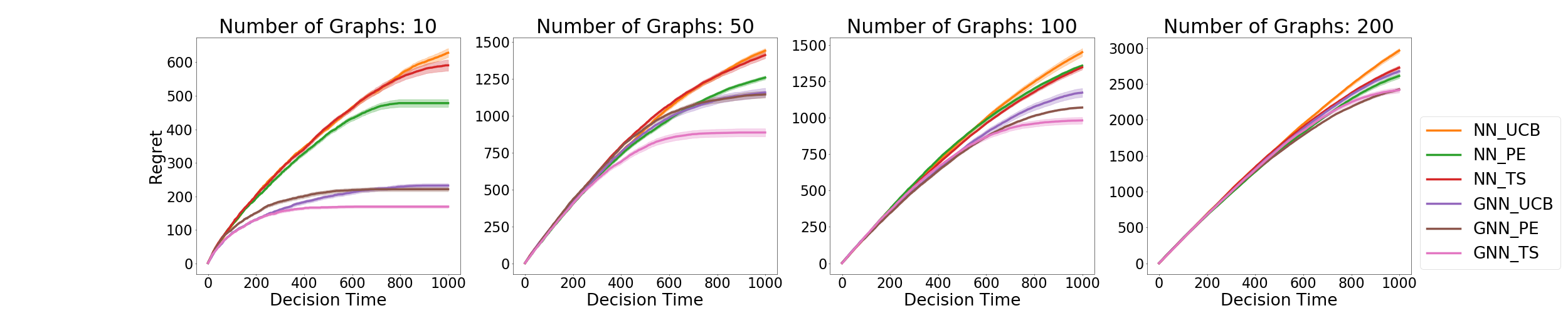
Figure 2: Competitive performance of GNN-TS is consistent across different sizes of graph space.

D.4 Effect of $m$ and Initial Gradients

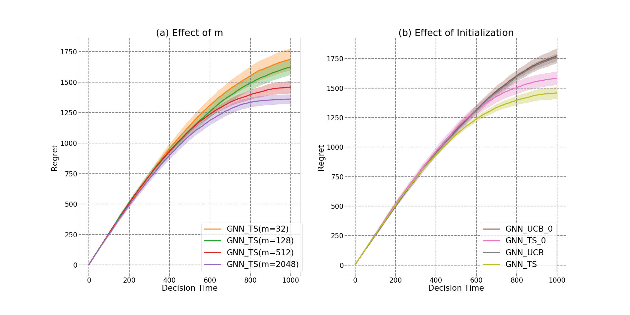
Figure 3: Increasing $m$ can improve the performance of GNN-TS and no improvement of using ${\boldsymbol{\textnormal{{g}}}}(G_{t};{\boldsymbol{\theta}}_{0})$.

Our regret analysis depends on the assumption that the width of the neural network $m$ must be large enough. We conduct an experiment to observe the effect from the width which is chosen from $\{32,128,512,2048\}$. As some previous works on Neural bandit use the gradients at initialization (${\boldsymbol{\textnormal{{g}}}}(G_{t};{\boldsymbol{\theta}}_{0})$) for uncertainty calculation [Zhou et al., 2020, Kassraie et al., 2022] while some works use ${\boldsymbol{\textnormal{{g}}}}(G_{t};{\boldsymbol{\theta}}_{t-1})$ which aligns with ours [Zhang et al., 2020]. Formally, instead of the update of uncertainty estimate in (5), using initial gradient means performing the following

$$\bar{\sigma}^{2}_{t}(G)=\frac{1}{m}\|{\boldsymbol{\textnormal{{g}}}}(G;{\boldsymbol{\theta}}_{0})\|_{\bar{{\boldsymbol{U}}}_{t}^{-1}}^{2},\qquad\bar{{\boldsymbol{U}}}_{t}=\bar{{\boldsymbol{U}}}_{t-1}+{\boldsymbol{\textnormal{{g}}}}(G_{t};{\boldsymbol{\theta}}_{0}){\boldsymbol{\textnormal{{g}}}}(G_{t};{\boldsymbol{\theta}}_{0})^{\top}/m.$$ (133)

Part (a) of Figure 3 reflects that the wider MLP has better performance which matches our expectation. Moreover, part (b) of Figure 3 reflects that there are no benefits from setting gradients used in algorithms to be the initial gradients for all $t\in[T]$. One small final observation is that the effects of $m$ and initialization are not strong.

D.5 Additional Figures and Tables

D.5.1 Results for Erdös–Rényi Random Graphs.

For better visualization of the $192$ synthetic data environments using Erdös–Rényi random graphs, we summarised the result in Table 1. The metrics are relative regret and top rate, which are defined based on regret as follow. The relative regret of one algorithm in one data environment is defined as

$$\text{Relative Regret:}\tilde{R}^{\text{alg, env}}=\frac{R_{T}^{\text{alg, env}}}{\max_{\text{alg}}R_{T}^{\text{alg, env}}}$$ (134)

where $R_{T}^{\text{alg, env}}$ is the cumulative regret of algorithm alg, and data environment env.

We define the top rate for the policy in algorithm as the number of times such that the policy achieve the least two cumulative regret $R_{T}$. The denomnator is the number of total trails, which is the $1920$, the $10$ repetition and $192$ combinations of ER environments. The top rate of one algorithm is defined as

$$\text{Top Rate:}\alpha_{\text{alg}}=\frac{\text{\# times \text{alg} achieves "Top 2"}}{\text{\# trails}}.$$ (135)

	NN-UCB	NN-PE	NN-TS	GNN-UCB	GNN-PE	GNN-TS
Top Rate ($\alpha_{\text{alg}}$)	$0.0\%$	$1.6\%$	$0.0\%$	$9.4\%$	$90.6\%$	98.4 %
Relative Regret ($\tilde{R}^{\text{alg, env}}$)	$0.994(0.02)$	$0.891(0.06)$	$0.943(0.05)$	$0.762(0.15)$	$0.690(0.14)$	0.595(0.16)

Table 1: Results on Erdös–Rényi random graphs. $192$ data environments with $10$ repetitions.

D.5.2 Results for Random Dot Product Graphs

We provide the experiment results for regret on all random dot product graph settings. In thee plots, different rows represents different sizes of the graph space ($|{\mathcal{G}}|$) and columns represents the choices of the number of nodes in the graph ($N$).

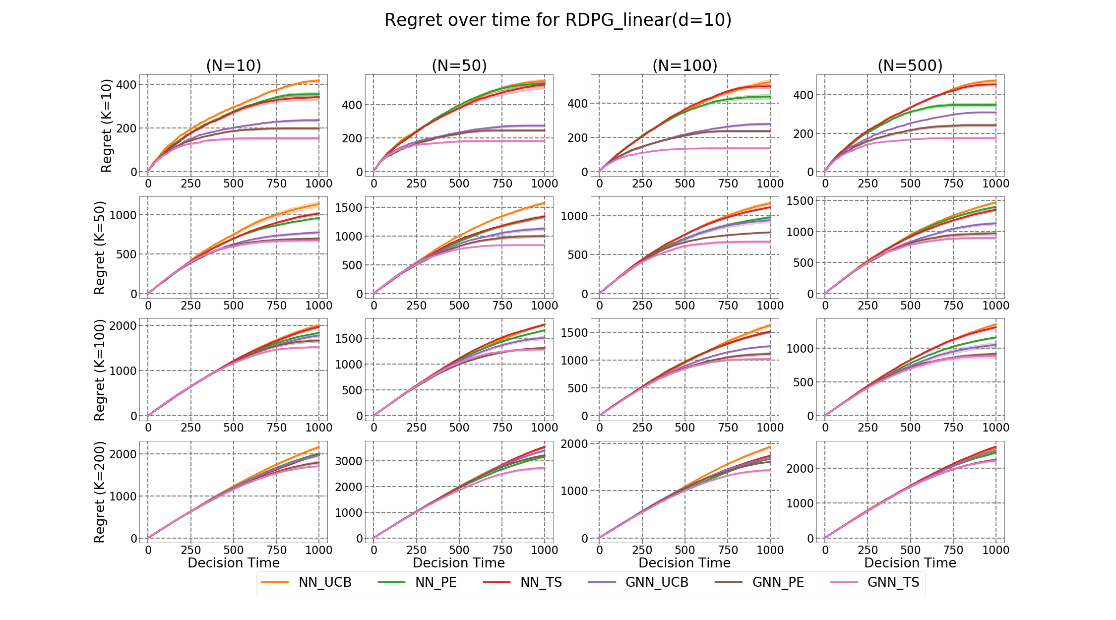
Figure 4: Random Dot Product Graphs with linear reward.

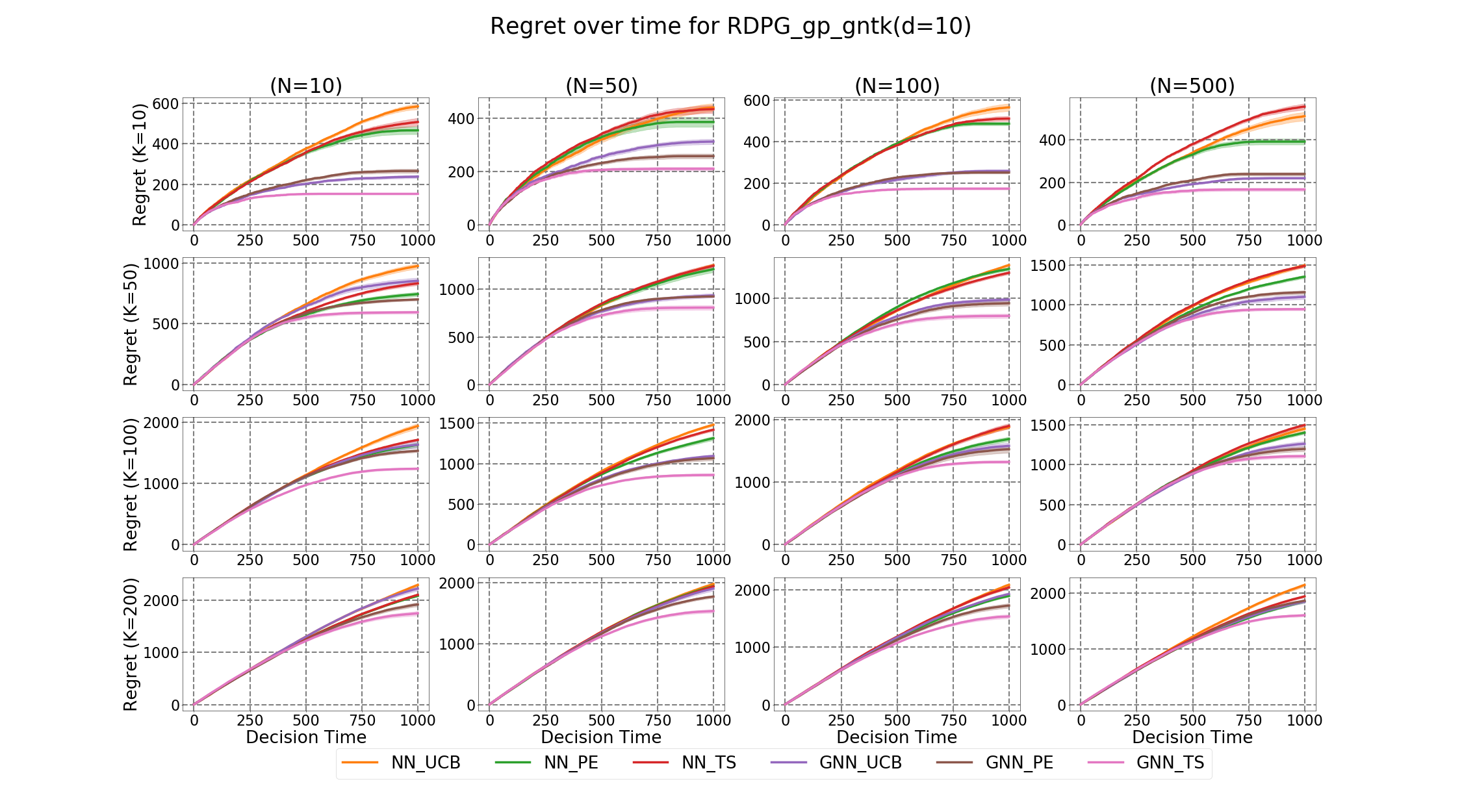
Figure 5: Random Dot Product Graphs with GP and GNTK for reward.

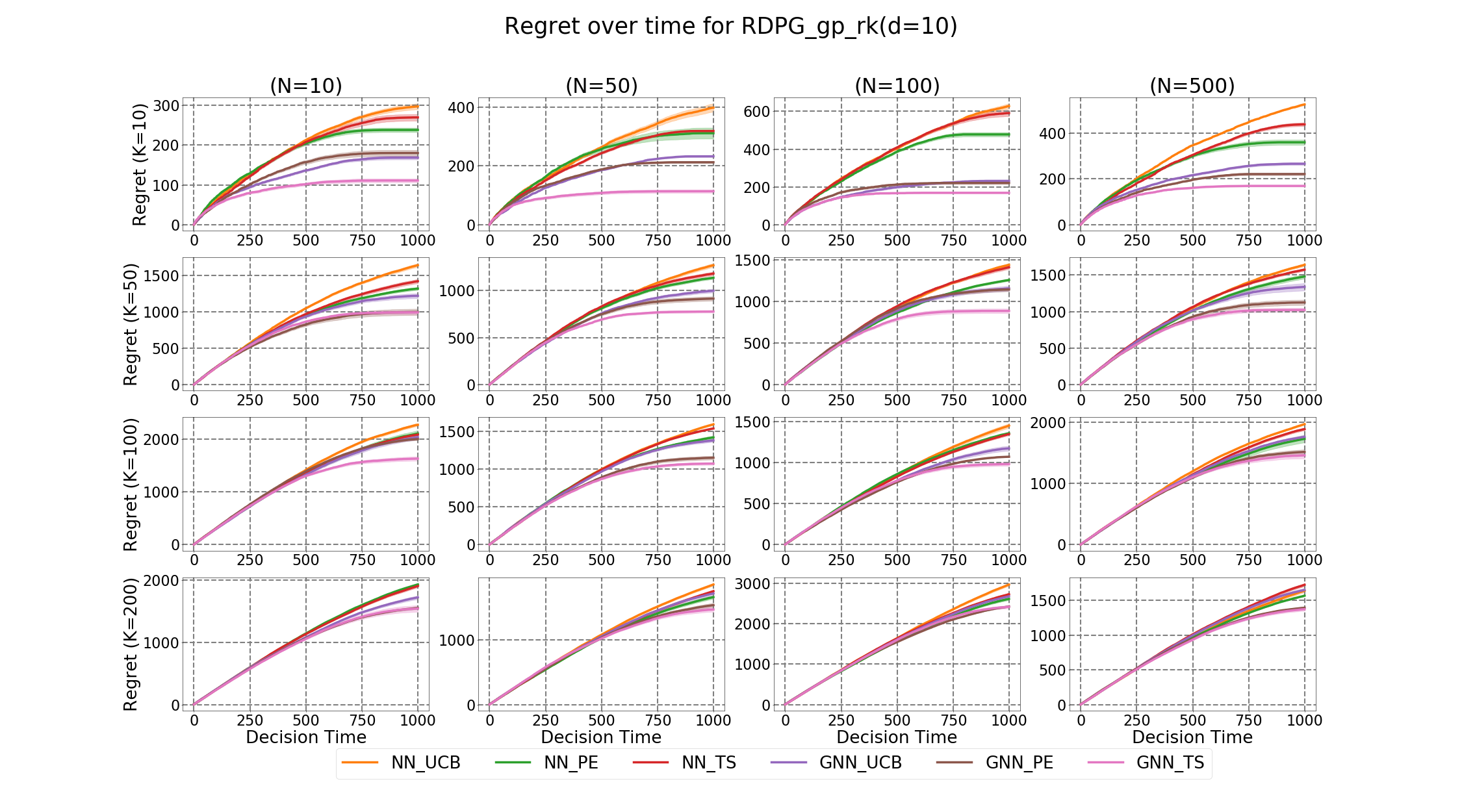
Figure 6: Random Dot Product Graphs with GP and representation kernel for reward.

References

- Abeille and Lazaric [2017] Marc Abeille and Alessandro Lazaric. Linear thompson sampling revisited. In Artificial Intelligence and Statistics, pages 176–184. PMLR, 2017.
- Agrawal and Goyal [2013] Shipra Agrawal and Navin Goyal. Thompson sampling for contextual bandits with linear payoffs. In International conference on machine learning, pages 127–135. PMLR, 2013.
- Arora et al. [2019] Sanjeev Arora, Simon S Du, Wei Hu, Zhiyuan Li, Russ R Salakhutdinov, and Ruosong Wang. On exact computation with an infinitely wide neural net. Advances in neural information processing systems, 32, 2019.
- Bellemare et al. [2019] Marc Bellemare, Will Dabney, Robert Dadashi, Adrien Ali Taiga, Pablo Samuel Castro, Nicolas Le Roux, Dale Schuurmans, Tor Lattimore, and Clare Lyle. A geometric perspective on optimal representations for reinforcement learning. Advances in neural information processing systems, 32, 2019.
- Bietti and Mairal [2019] Alberto Bietti and Julien Mairal. On the inductive bias of neural tangent kernels. Advances in Neural Information Processing Systems, 32, 2019.
- Chapelle and Li [2011] Olivier Chapelle and Lihong Li. An empirical evaluation of thompson sampling. Advances in neural information processing systems, 24, 2011.
- Chen et al. [2021] Houshuang Chen, Shuai Li, Chihao Zhang, et al. Understanding bandits with graph feedback. Advances in Neural Information Processing Systems, 34:24659–24669, 2021.
- Chowdhury and Gopalan [2017] Sayak Ray Chowdhury and Aditya Gopalan. On kernelized multi-armed bandits. In International Conference on Machine Learning, pages 844–853. PMLR, 2017.
- Dai et al. [2022] Zhongxiang Dai, Yao Shu, Bryan Kian Hsiang Low, and Patrick Jaillet. Sample-then-optimize batch neural thompson sampling. Advances in Neural Information Processing Systems, 35:23331–23344, 2022.
- Dann et al. [2020] Christoph Dann, Yishay Mansour, Mehryar Mohri, Ayush Sekhari, and Karthik Sridharan. Reinforcement learning with feedback graphs. Advances in Neural Information Processing Systems, 33:16868–16878, 2020.
- Esposito et al. [2022] Emmanuel Esposito, Federico Fusco, Dirk van der Hoeven, and Nicolò Cesa-Bianchi. Learning on the edge: Online learning with stochastic feedback graphs. Advances in Neural Information Processing Systems, 35:34776–34788, 2022.
- Gómez-Bombarelli et al. [2018] Rafael Gómez-Bombarelli, Jennifer N Wei, David Duvenaud, José Miguel Hernández-Lobato, Benjamín Sánchez-Lengeling, Dennis Sheberla, Jorge Aguilera-Iparraguirre, Timothy D Hirzel, Ryan P Adams, and Alán Aspuru-Guzik. Automatic chemical design using a data-driven continuous representation of molecules. ACS central science, 4(2):268–276, 2018.
- Gou et al. [2023] Yutian Gou, Jinfeng Yi, and Lijun Zhang. Stochastic graphical bandits with heavy-tailed rewards. In Uncertainty in Artificial Intelligence, pages 734–744. PMLR, 2023.
- Griffiths and Hernández-Lobato [2020] Ryan-Rhys Griffiths and José Miguel Hernández-Lobato. Constrained bayesian optimization for automatic chemical design using variational autoencoders. Chemical science, 11(2):577–586, 2020.
- Gu et al. [2024] Quanquan Gu, Amin Karbasi, Khashayar Khosravi, Vahab Mirrokni, and Dongruo Zhou. Batched neural bandits. ACM/IMS Journal of Data Science, 1(1):1–18, 2024.
- Idé et al. [2022] Tsuyoshi Idé, Keerthiram Murugesan, Djallel Bouneffouf, and Naoki Abe. Targeted advertising on social networks using online variational tensor regression. arXiv preprint arXiv:2208.10627, 2022.
- Jacot et al. [2018] Arthur Jacot, Franck Gabriel, and Clément Hongler. Neural tangent kernel: Convergence and generalization in neural networks. Advances in neural information processing systems, 31, 2018.
- Jin et al. [2018] Wengong Jin, Regina Barzilay, and Tommi Jaakkola. Junction tree variational autoencoder for molecular graph generation. In International conference on machine learning, pages 2323–2332. PMLR, 2018.
- Kassraie and Krause [2022] Parnian Kassraie and Andreas Krause. Neural contextual bandits without regret. In International Conference on Artificial Intelligence and Statistics, pages 240–278. PMLR, 2022.
- Kassraie et al. [2022] Parnian Kassraie, Andreas Krause, and Ilija Bogunovic. Graph neural network bandits. Advances in Neural Information Processing Systems, 35:34519–34531, 2022.
- Kawale et al. [2015] Jaya Kawale, Hung H Bui, Branislav Kveton, Long Tran-Thanh, and Sanjay Chawla. Efficient thompson sampling for online matrix-factorization recommendation. Advances in neural information processing systems, 28, 2015.
- Kim and Tewari [2019] Baekjin Kim and Ambuj Tewari. On the optimality of perturbations in stochastic and adversarial multi-armed bandit problems. Advances in Neural Information Processing Systems, 32, 2019.
- Kocák et al. [2014] Tomáš Kocák, Michal Valko, Rémi Munos, and Shipra Agrawal. Spectral thompson sampling. In Proceedings of the AAAI Conference on Artificial Intelligence, volume 28, 2014.
- Kocák et al. [2020] Tomáš Kocák, Rémi Munos, Branislav Kveton, Shipra Agrawal, and Michal Valko. Spectral bandits. The Journal of Machine Learning Research, 21(1):9003–9046, 2020.
- Kong et al. [2022] Fang Kong, Yichi Zhou, and Shuai Li. Simultaneously learning stochastic and adversarial bandits with general graph feedback. In International Conference on Machine Learning, pages 11473–11482. PMLR, 2022.
- Korovina et al. [2020] Ksenia Korovina, Sailun Xu, Kirthevasan Kandasamy, Willie Neiswanger, Barnabas Poczos, Jeff Schneider, and Eric Xing. Chembo: Bayesian optimization of small organic molecules with synthesizable recommendations. In International Conference on Artificial Intelligence and Statistics, pages 3393–3403. PMLR, 2020.
- Kveton et al. [2019a] Branislav Kveton, Csaba Szepesvari, Mohammad Ghavamzadeh, and Craig Boutilier. Perturbed-history exploration in stochastic multi-armed bandits. arXiv preprint arXiv:1902.10089, 2019a.
- Kveton et al. [2019b] Branislav Kveton, Csaba Szepesvari, Mohammad Ghavamzadeh, and Craig Boutilier. Perturbed-history exploration in stochastic linear bandits. arXiv preprint arXiv:1903.09132, 2019b.
- Kveton et al. [2020] Branislav Kveton, Manzil Zaheer, Csaba Szepesvari, Lihong Li, Mohammad Ghavamzadeh, and Craig Boutilier. Randomized exploration in generalized linear bandits. In International Conference on Artificial Intelligence and Statistics, pages 2066–2076. PMLR, 2020.
- Lattimore and Szepesvári [2020] Tor Lattimore and Csaba Szepesvári. Bandit algorithms. Cambridge University Press, 2020.
- Lee et al. [2020] Chung-Wei Lee, Haipeng Luo, and Mengxiao Zhang. A closer look at small-loss bounds for bandits with graph feedback. In Conference on Learning Theory, pages 2516–2564. PMLR, 2020.
- Liu et al. [2018] Fang Liu, Zizhan Zheng, and Ness Shroff. Analysis of thompson sampling for graphical bandits without the graphs. arXiv preprint arXiv:1805.08930, 2018.
- Lykouris et al. [2020] Thodoris Lykouris, Eva Tardos, and Drishti Wali. Feedback graph regret bounds for thompson sampling and ucb. In Algorithmic Learning Theory, pages 592–614. PMLR, 2020.
- Nguyen-Tang et al. [2021] Thanh Nguyen-Tang, Sunil Gupta, A Tuan Nguyen, and Svetha Venkatesh. Offline neural contextual bandits: Pessimism, optimization and generalization. arXiv preprint arXiv:2111.13807, 2021.
- Qi et al. [2022] Yunzhe Qi, Yikun Ban, and Jingrui He. Neural bandit with arm group graph. In Proceedings of the 28th ACM SIGKDD Conference on Knowledge Discovery and Data Mining, pages 1379–1389, 2022.
- Qi et al. [2023] Yunzhe Qi, Yikun Ban, and Jingrui He. Graph neural bandits. In Proceedings of the 29th ACM SIGKDD Conference on Knowledge Discovery and Data Mining, pages 1920–1931, 2023.
- Riquelme et al. [2018] Carlos Riquelme, George Tucker, and Jasper Snoek. Deep bayesian bandits showdown: An empirical comparison of bayesian deep networks for thompson sampling. arXiv preprint arXiv:1802.09127, 2018.
- Russo et al. [2018] Daniel J Russo, Benjamin Van Roy, Abbas Kazerouni, Ian Osband, Zheng Wen, et al. A tutorial on thompson sampling. Foundations and Trends® in Machine Learning, 11(1):1–96, 2018.
- Srinivas et al. [2009] Niranjan Srinivas, Andreas Krause, Sham M Kakade, and Matthias Seeger. Gaussian process optimization in the bandit setting: No regret and experimental design. arXiv preprint arXiv:0912.3995, 2009.
- Thaker et al. [2022] Parth Thaker, Mohit Malu, Nikhil Rao, and Gautam Dasarathy. Maximizing and satisficing in multi-armed bandits with graph information. Advances in Neural Information Processing Systems, 35:2019–2032, 2022.
- Thompson [1933] William R Thompson. On the likelihood that one unknown probability exceeds another in view of the evidence of two samples. Biometrika, 25(3-4):285–294, 1933.
- Toni and Frossard [2023] Laura Toni and Pascal Frossard. Online network source optimization with graph-kernel mab. In Joint European Conference on Machine Learning and Knowledge Discovery in Databases, pages 242–258. Springer, 2023.
- Tossou et al. [2017] Aristide Tossou, Christos Dimitrakakis, and Devdatt Dubhashi. Thompson sampling for stochastic bandits with graph feedback. In Proceedings of the AAAI Conference on Artificial Intelligence, volume 31, 2017.
- Upadhyay et al. [2020] Sohini Upadhyay, Mikhail Yurochkin, Mayank Agarwal, Yasaman Khazaeni, and Djallel Bouneffouf. Graph convolutional network upper confident bound. 2020.
- Vakili et al. [2021] Sattar Vakili, Nacime Bouziani, Sepehr Jalali, Alberto Bernacchia, and Da-shan Shiu. Optimal order simple regret for gaussian process bandits. Advances in Neural Information Processing Systems, 34:21202–21215, 2021.
- Valko et al. [2013] Michal Valko, Nathaniel Korda, Rémi Munos, Ilias Flaounas, and Nelo Cristianini. Finite-time analysis of kernelised contextual bandits. arXiv preprint arXiv:1309.6869, 2013.
- Wang-Henderson et al. [2023a] Miles Wang-Henderson, Bartu Soyuer, Parnian Kassraie, Andreas Krause, and Ilija Bogunovic. Graph neural network powered bayesian optimization for large molecular spaces. In ICML 2023 Workshop on Structured Probabilistic Inference & Generative Modeling, 2023a.
- Wang-Henderson et al. [2023b] Miles Wang-Henderson, Bartu Soyuer, Parnian Kassraie, Andreas Krause, and Ilija Bogunovic. Graph neural bayesian optimization for virtual screening. In NeurIPS 2023 Workshop on Adaptive Experimental Design and Active Learning in the Real World, 2023b.
- Waradpande et al. [2020] Vikram Waradpande, Daniel Kudenko, and Megha Khosla. Deep reinforcement learning with graph-based state representations. arXiv preprint arXiv:2004.13965, 2020.
- Weininger [1988] David Weininger. Smiles, a chemical language and information system. 1. introduction to methodology and encoding rules. Journal of chemical information and computer sciences, 28(1):31–36, 1988.
- Wu et al. [2022] Shuang Wu, Chi-Hua Wang, Yuantong Li, and Guang Cheng. Residual bootstrap exploration for stochastic linear bandit. In Uncertainty in Artificial Intelligence, pages 2117–2127. PMLR, 2022.
- Xu et al. [2020] Pan Xu, Zheng Wen, Handong Zhao, and Quanquan Gu. Neural contextual bandits with deep representation and shallow exploration. arXiv preprint arXiv:2012.01780, 2020.
- Yang et al. [2020] Kaige Yang, Laura Toni, and Xiaowen Dong. Laplacian-regularized graph bandits: Algorithms and theoretical analysis. In International Conference on Artificial Intelligence and Statistics, pages 3133–3143. PMLR, 2020.
- Yang and Wang [2020] Lin Yang and Mengdi Wang. Reinforcement learning in feature space: Matrix bandit, kernels, and regret bound. In International Conference on Machine Learning, pages 10746–10756. PMLR, 2020.
- Yu et al. [2020] Tong Yu, Branislav Kveton, Zheng Wen, Ruiyi Zhang, and Ole J Mengshoel. Graphical models meet bandits: A variational thompson sampling approach. In International Conference on Machine Learning, pages 10902–10912. PMLR, 2020.
- Zahavy and Mannor [2019] Tom Zahavy and Shie Mannor. Deep neural linear bandits: Overcoming catastrophic forgetting through likelihood matching. arXiv preprint arXiv:1901.08612, 2019.
- Zhang et al. [2020] Weitong Zhang, Dongruo Zhou, Lihong Li, and Quanquan Gu. Neural thompson sampling. arXiv preprint arXiv:2010.00827, 2020.
- Zhou et al. [2020] Dongruo Zhou, Lihong Li, and Quanquan Gu. Neural contextual bandits with ucb-based exploration. In International Conference on Machine Learning, pages 11492–11502. PMLR, 2020.