Quantum Equation-of-Motion Method with Single, Double, and Triple Excitations

Abstract

The quantum equation-of-motion (qEOM) method with singles and doubles has been suggested to study electronically excited states while it fails to predict the excitation energies dominated by double excitations. In this work, we present an efficient implementation of the qEOM method with single, double and triple excitations. In order to reduce the computational complexity, we utilize the point group symmetry and perturbation theory to screen triple excitation operators, and the scaling is reduced from $N_{o}^{6}N_{v}^{6}$ to $N_{o}^{5}N_{v}^{5}$. Furthermore, we introduce a perturbation correction to the excitation energy to account for the effect of ignored triple excitation operators. We apply this method to study challenging cases, for which the qEOM-SD method exhibits large errors, such as the 2 ${}^{1}\Delta$ excited state of $\rm{CH}^{+}$ and the 2 ${}^{1}\Sigma$ state of $\rm{H}_{8}$ molecule. Our new method yields the energy errors less than 0.18 eV.

Hefei National Laboratory, University of Science and Technology of China, Hefei 230088, China Hefei National Laboratory, University of Science and Technology of China, Hefei 230088, China

1 Introduction

Accurate prediction of excited-state properties has broad implications for many important real-world scenarios, such as the design of organic light-emitting diodes and the study of photosynthesis reaction mechanisms, while posing a significant challenge for classical computing with (near-) exact approaches due to unfavorable computational scaling ^{1, 2, 3, 4}. The emergence of quantum computing provides a new paradigm to solve the Schrödinger equation in an accurate and efficient manner by utilizing quantum superposition and entanglement, where $N$ qubits can represent a quantum state of $2^{N}$ dimensions ^{5, 6, 7, 8, 9}. It is therefore necessary to explore carrying out excited-state simulations on quantum computers.

In recent years, many quantum algorithms have emerged for finding electronically excited states of a given Hamiltonian ^{10, 11, 12, 13, 14, 15}. In this regard, the Hamiltonian simulation algorithms, including quantum phase estimation ^{16, 17}, quantum Krylov subspace expansion ¹³ and quantum Lanczos recursion ¹⁸, are a straightforward way to implement excited-state simulations. However, these algorithms require to apply the Hamiltonian $\hat{H}$ or $e^{-i\hat{H}t}$ many times onto a quantum state, resulting in deep quantum circuits. Additionally, these algorithms are generally sensitive to noise in quantum systems so that it is difficult to obtain reliable results due to error accumulation. As such, they are considered as long-term algorithms to implement on a fault-tolerant quantum computer.

Given near-term quantum devices limited by the coherence time and the fidelity of quantum gates ^{19, 20}, variational quantum eigensolver (VQE) ⁶, known as a hybrid quantum-classical algorithm that has features of low circuit depth and robust noise resilience, is one of the most widely used algorithms for electronic structure simulations. Various excited-state methods have been also developed based on the VQE algorithm. One simple way to extend the VQE to find excited states is to optimize parameterized quantum circuits (PQC) under certain constrained conditions. For examples, the variational quantum deflation algorithm ^{21, 22} adds a penalty function to the original Hamiltonian in the VQE so that the $(k+1)$th eigenstate is optimized to be orthogonal to all previously computed $k$ eigenstates. The folded spectrum method ⁶ minimizes an objective function $\langle(\hat{H}-E_{\lambda})^{2}\rangle$ to find a certain eigenstate with the energy closest to $E_{\lambda}$. In contrast to the above two algorithms, the subspace search VQE algorithm ¹¹ tries to obtain the lowest-lying $k$ eigenstates simultaneously, which are represented by applying an ansatz circuit onto $k$ orthogonal initial states. Witness-assisted variational eigenspectra solver ²³ utilizes an additional qubit, known as a witness qubit, to monitor the quantum circuit’s output and determines whether it is the target excited state. The major challenge faced by PQC-based approaches is the high-dimension nonlinear optimization problem as the number of circuit parameters increases. In case of excited-state calculations, it is also a challenge task to find the target state because the optimization procedure may get stuck in other states ^{24, 11}.

Alternatively, one can employ diagonalization methods to extract multiple low-lying eigenstates of a given Hamiltonian. A typical example is the quantum subspace expansion (QSE) algorithm, which prepares an approximate ground state in a small active space and then expands the ground state and excited states with the same subspace ²⁵. In contrast, Ollitrault et al. ²⁶ proposed the quantum equation-of-motion (qEOM) method for excited-state calculations. The qEOM employs the unitary coupled-cluster (UCC) ansatz to represent the ground state and expands the excited-state wave functions as a linear combination of basis functions commonly generated by applying single and double excitation operators onto the ground state. Since the qEOM fails to satisfy the killer condition, it leads to significant errors when used to calculate vertical ionization potentials (IPs) and electron affinities (EAs). To address this issue, qEOM was extended to quantum self-consistent equation-of-motion (q-sc-EOM) ²⁷. In the q-sc-EOM, the excitation operator manifold is rotated, meaning that the excitation operators undergo a similarity transformation using the optimized UCC operator to satisfy the killer condition. In addition, the q-sc-EOM employs the adaptive derivative-assembled pseudotrotter (ADAPT) ansatz to generate the accurate ground-state wave function for small molecules.

Analogous to the classical EOM approaches, the computational accuracy of quantum EOM approaches also depends on the truncation of excitation operators. As stated in previous works, the EOM coupled cluster with singles and doubles (CCSD) method introduced significant errors when computing excited states dominated by double excitation components and excited-state potential energy surfaces (PESs) involving bond breaking. For example, the energy error for the $2\,^{1}\Delta$ state of the $\rm CH^{+}$ ion is as high as 3.946 eV, while the energy error for the $1\,^{1}\Delta_{g}$ state of the $\rm C_{2}$ molecule reaches 2.068 eV  ^{28, 29}. In this work, we found that the errors of the qEOM unitary CCSD (qEOM-UCCSD) are within the same order of magnitude as EOM-CCSD. Thus, in order to improve the computational accuracy, it is necessary to consider higher-order excitation operators.

In this work, we extend the qEOM-SD algorithm to include triple excitations via many-body perturbation theory, resulting in the qEOM-SD(t) method. This method leverages orbital symmetries and perturbation theory to identify and eliminate redundant excitation operators. Furthermore, it replaces the effects of discarded excitation operators on excitation energies with their associated first-order perturbation energies. We test this method on $\rm CH^{+}$, HF, and $\rm H_{8}$, demonstrating significant improvements over the qEOM-SD method. Additionally, we extend the QSE algorithm to include triple excitations, introducing the QSE-SD(t) method, and compare it with the qEOM-SD(t).

2 Methodology

2.1 ADAPT-VQE algorithm

The ADAPT-VQE algorithm is utilized to generate the ground-state wave function ³⁰

$$|\psi_{0}\rangle=|\psi_{\rm VQE}\rangle=\hat{U}(\mathbf{\theta})|\psi_{\rm HF}\rangle=\prod\limits_{k=0}^{K}\hat{U}(\theta_{k})|\psi_{\rm HF}\rangle$$ (1)

where $|\psi_{\rm HF}\rangle$ is the Hartree-Fock state and the unitary transformation $\hat{U}(\theta_{k})$ is in the form of

$$\hat{U}(\theta_{k})=e^{\theta_{k}\hat{\tau}_{k}}$$ (2)

with $\hat{\tau}_{k}=\hat{T}_{k}-\hat{T}_{k}^{\dagger}$ being an anti-Hermitian operator. The operator pool $\mathcal{O}=\{\hat{T}_{k}\}$ is often assumed to be composed of all single and double excitation operators

$$\begin{split}&\hat{T}_{i}^{a}=\hat{a}_{a}^{\dagger}\hat{a}_{i}\\ &\hat{T}_{ij}^{ab}=\hat{a}_{a}^{\dagger}\hat{a}_{b}^{\dagger}\hat{a}_{j}\hat{a}_{i}\end{split}$$ (3)

In this work, we employ single and double excitation operators in the ADAPT-VQE calculations. The wave function of Eq. (1) is iteratively determined

$$|\psi^{(k)}\rangle=e^{\theta_{k}\hat{\tau}_{k}}|\psi^{(k-1)}\rangle,$$ (4)

where the operator $\hat{\tau}_{k}$ has the largest residual gradient $g_{k}=\max\limits_{\mu\in\mathcal{O}}g_{\mu}$ with

$$g_{\mu}=\left.\frac{\partial\langle\psi^{(k-1)}|e^{\theta\hat{\tau}^{\dagger}}\hat{H}e^{\theta\hat{\tau}}|\psi^{(k-1)}\rangle}{\partial\theta}\right|_{\hat{\tau}=\hat{\tau}_{\mu},\theta=0}$$ (5)

with respect to the wave function $|\psi^{(k-1)}\rangle$. In each iteration, variational parameters are optimized using the variational principle

$$E^{(k)}=\mathop{\min}_{\bm{\theta}}E^{(k)}(\bm{\theta})=\frac{\langle\psi^{(k)}(\bm{\theta})|H|\psi^{(k)}(\bm{\theta})\rangle}{\langle\psi^{(k)}(\bm{\theta})|\psi^{(k)}(\bm{\theta})\rangle}$$ (6)

When the norm of residual gradients is smaller than a threshold $\epsilon$

$$\sqrt{\sum_{\mu}|g_{\mu}|^{2}}<\epsilon,$$ (7)

the iterative optimization procedure is finished.

2.2 Quantum equation-of-motion method

The EOM theory introduce an excitation operator $\hat{R}_{m}$ to define the $m$th excited state wave function

$$|\psi_{m}\rangle=\hat{R}_{m}|\psi_{0}\rangle,$$ (8)

and the excitation operator satisfies the EOM equation

$$[\hat{H},\hat{R}_{m}]=\omega_{m}\hat{R}_{m}$$ (9)

where $\omega_{m}$ is the mth vertical excitation energy. The excitation operator $\hat{R}_{m}$ should in principle satisfy the killer condition or the vacuum annihilation condition (VAC)

$$\hat{R}_{m}^{\dagger}|\psi_{\rm 0}\rangle=0,$$ (10)

implying that the ground state cannot be de-excited. In the EOM-CC theory, an effective Hamiltonian

$$\bar{H}=e^{-\hat{T}}\hat{H}e^{\hat{T}}$$ (11)

is defined and the reference state $|\psi_{0}\rangle=|\psi_{\rm HF}\rangle$. Here, $\hat{T}=\sum_{ai}\hat{T}^{a}_{i}+\frac{1}{4}\sum_{abij}\hat{T}^{ab}_{ij}+\cdots$. As such, the VAC is always satisfied if the excitation operators are restricted to promote electrons from occupied to virtual orbitals.

Inspired by the EOM-CC theory, one can construct an effective Hamiltonian using the unitary transformation $\hat{U}$ in Eq. (1) as

$$\bar{H}=\hat{U}^{\dagger}\hat{H}\hat{U}$$ (12)

and the ground-state energy is rewritten as

$$E_{0}=\langle\psi_{\rm HF}|\bar{H}|\psi_{\rm HF}\rangle.$$ (13)

As such, the mth excited state is defined as

$$|\psi_{m}\rangle=\hat{R}_{m}|\psi_{\rm HF}\rangle$$ (14)

with respect to the effective Hamiltonian of Eq. (12). In this work, $\hat{R}_{m}$ is approximated as the linear combination of single, double and triple excitations

$$\begin{split}\hat{R}_{m}&=\sum_{ia}\gamma_{i}^{a}\hat{a}_{a}^{{\dagger}}\hat{a}_{i}+\sum_{ijab}\gamma_{ij}^{ab}\hat{a}_{a}^{{\dagger}}\hat{a}_{b}^{{\dagger}}\hat{a}_{i}\hat{a}_{j}+\sum_{ijkabc}\gamma_{ijk}^{abc}\hat{a}_{a}^{{\dagger}}\hat{a}_{b}^{{\dagger}}\hat{a}_{c}^{{\dagger}}\hat{a}_{i}\hat{a}_{j}\hat{a}_{k}\\ &=\sum_{I}\gamma_{I}\hat{r}_{I}\end{split}$$ (15)

where $i$, $j$ and $k$ represent occupied spin orbitals, $a$, $b$ and $c$ represent virtual spin orbitals. We name this method qEOM-SDT. It is clear that the VAC is also satisfied when one consider the Hartree-Fock state as the reference state.

Analogous to the EOM-CC theory, the working equation of the qEOM theory is formulated as

$$\langle\psi_{\rm HF}|\hat{r}_{I}^{{\dagger}}[\bar{H},\hat{R}_{m}]|\psi_{\rm HF}\rangle=\omega_{m}\langle\psi_{\rm HF}|\hat{r}_{I}^{{\dagger}}\hat{R}_{m}|\psi_{\rm HF}\rangle$$ (16)

After some rearrangements, the eigenvalue equation is formulated as

$$\bm{M\Gamma}_{m}=\omega_{m}\bm{\Gamma}_{m}$$ (17)

with $\omega_{m}$ is the vertical excitation energy defined as the energy difference between the ground state and the mth excited state. The matrix elements of $\bm{M}$ is

$$\bm{M}_{I,J}=\langle{\psi_{\rm HF}}|\hat{r}_{I}^{\dagger}(\bar{H}-E_{0})\hat{r}_{J}|{\psi_{\rm HF}}\rangle$$ (18)

The coefficients $\bm{\Gamma}_{m}=\{\gamma_{i}^{a},\gamma_{ij}^{ab},\gamma_{ijk}^{abc}\}$ in $\hat{R}_{m}$ can be obtained by diagonalizing Eq. (17). Note that Eq. (17) is the same as the eigenvalue equation proposed in the q-sc-EOM approach ²⁷.

2.3 qEOM-SDt method

The number of triple excitation operators scales as $N_{o}^{3}N_{v}^{3}$ with $N_{o}$ and $N_{v}$ being the number of occupied and virtual spin orbitals. As such, the major computational bottleneck of qEOM-SDT results from evaluating the matrix elements of $\bm{M}$ related to the triple excitations, scaling as $N_{o}^{6}N_{v}^{6}$. Here, we exploit molecular orbital symmetry and the perturbation theory to reduce the computational complexity.

(1) Symmetry Preserving in ADAPT-VQE

As discussed in Ref. ³¹, when the ground state is non-degenerate, its irreducible representation (Irrep) is in principle the same as the reference state. As such, in the ADAPT-VQE calculation, we have

$${\rm Irrep}(|{\psi_{\rm VQE}}\rangle)={\rm Irrep}(|{\psi_{\rm HF}}\rangle)$$ (19)

Since the Hartree-Fock state cannot be de-excited, the above condition is equivalent to the following one:

$${\rm Irrep}(\hat{T}_{i}|{\psi_{\rm HF}\rangle})=\rm Irrep(|\psi_{HF}\rangle)$$ (20)

This condition can serve as a guideline for building the operator pool in the ADAPT-VQE algorithm. The detailed derivation of Eq. (20) is provided in Appendix.

(2) Block Diagonalization

The $\bm{M}$ is the matrix representation of $\bar{H}$ in the subspace $\{\hat{r}_{1}|{\psi_{\rm HF}}\rangle,\hat{r}_{2}|{\psi_{\rm HF}}\rangle,\hat{r}_{3}|{\psi_{\rm HF}}\rangle,\cdots\}$. Here, $\hat{r}_{I}\in\hat{\mathbf{R}}$, where $\hat{\mathbf{R}}=\hat{\mathbf{R}}_{1}\cup\hat{\mathbf{R}}_{2}\cup\hat{\mathbf{R}}_{3}$, $\hat{\mathbf{R}}_{1}=\{\hat{a}_{a}^{\dagger}\hat{a}_{i}\}$, $\hat{\mathbf{R}}_{2}=\{\hat{a}_{a}^{\dagger}\hat{a}_{b}^{\dagger}\hat{a}_{i}\hat{a}_{j}\}$ and $\hat{\mathbf{R}}_{3}=\{\hat{a}_{a}^{\dagger}\hat{a}_{b}^{\dagger}\hat{a}_{c}^{\dagger}\hat{a}_{i}\hat{a}_{j}\hat{a}_{k}\}$. As the unitary transformation $\hat{U}$ determined in the VQE will not change the irreducible representation of the reference configuration state, it belongs to the totally symmetric irreducible representation, such as $A_{\mathrm{g}}$ in $D_{2h}$ group and $A_{1}$ in $C_{2v}$ group. According to the group theory ³², the Hamiltonian $\hat{H}$ belongs to the totally symmetric irreducible representation. If bra $\hat{U}\hat{r}_{I}|{\psi_{\rm HF}}\rangle$ and ket $\hat{U}\hat{r}_{J}|{\psi_{\rm HF}}\rangle$ on both sides of $\hat{H}$ have different irreducible representations, the matrix element $\bm{M}_{I,J}$ is zero. This reveals that we can implement a block diagonalization of the eigenvalue equation of Eq. (17) for excited states per irreducible representation

$${\rm Irrep}(\hat{r}_{I}|{\psi_{\rm HF}\rangle})={\rm Irrep}(|\psi_{m}\rangle)$$ (21)

(3) Screening Triple Excitation Operators via the Perturbation Theory

We assume that the zero-order of $m$th excited state for the effective Hamiltonian $\bar{H}$ is only formed by single and double excitations

$${|\psi_{m}^{(0)}\rangle}=\sum_{\begin{subarray}{c}\hat{r}_{I}\in{\hat{\mathbf{R}}_{1}\cup\hat{\mathbf{R}}_{2}}\end{subarray}}\gamma_{I}\hat{r}_{I}|\psi_{\rm HF}\rangle$$ (22)

and the first-order wave function is defined as

$${|\psi_{m}^{(1)}\rangle}=\sum_{\begin{subarray}{c}\hat{r}_{I}\in{\hat{\mathbf{R}}_{3}}\end{subarray}}\gamma_{I}\hat{r}_{I}|\psi_{\rm HF}\rangle$$ (23)

So

$${|\psi_{m}\rangle}=|\psi_{m}^{(0)}\rangle+|\psi_{m}^{(1)}\rangle$$ (24)

$$E_{m}\approx E_{m}^{(0)}+E_{m}^{(1)}$$ (25)

And $E_{m}^{(0)}=\langle{\psi_{m}^{(0)}}|\bar{H}|\psi_{m}^{(0)}\rangle$. Substituting Eq. (24) and (25) into $\bar{H}|\psi_{m}\rangle=E_{m}|\psi_{m}\rangle$, and ignoring high-order term $E_{m}^{(1)}|\psi_{m}^{(1)}\rangle$, we get

$$\bar{H}(|\psi_{m}^{(0)}\rangle+|\psi_{m}^{(1)}\rangle)=(E_{m}^{(0)}+E_{m}^{(1)})|\psi_{m}^{(0)}\rangle+E_{m}^{(0)}|\psi_{m}^{(1)}\rangle$$ (26)

Left-multiplying Eq. (26) by $\langle\psi_{\rm HF}|\hat{r}_{J}^{\dagger}$, where $\hat{r}_{J}\in\hat{\mathbf{R}}_{3}$ is a crucial point to note, we obtain

$$\langle\psi_{\rm HF}|\hat{r}_{J}^{\dagger}\bar{H}|\psi_{m}^{(0)}\rangle+\langle\psi_{\rm HF}|\hat{r}_{J}^{\dagger}\bar{H}(\sum_{\begin{subarray}{c}\hat{r}_{I}\in{\hat{\mathbf{R}}_{3}}\end{subarray}}\gamma_{I}\hat{r}_{I})|\psi_{\rm HF}\rangle=E_{m}^{(0)}\gamma_{J}$$ (27)

since $\langle\psi_{\rm HF}|\hat{r}_{J}^{\dagger}|\psi_{m}^{(0)}\rangle=0$. Considering the diagonal approximation, i.e., $\langle\psi_{\rm HF}|\hat{r}_{J}^{\dagger}\bar{H}\hat{r}_{I}|\psi_{\rm HF}\rangle\approx\delta_{IJ}\langle\psi_{\rm HF}|r_{J}^{\dagger}\bar{H}\hat{r}_{J}|\psi_{\rm HF}\rangle$,

$$\gamma_{J}=\frac{\langle\psi_{\rm HF}|\hat{r}_{J}^{\dagger}\bar{H}|\psi_{m}^{(0)}\rangle}{E_{m}^{(0)}-\langle\psi_{\rm HF}|\hat{r}_{J}^{\dagger}\bar{H}\hat{r}_{J}|\psi_{\rm HF}\rangle}$$ (28)

Left-multiplying Eq. (26) by $\langle\psi_{m}^{(0)}|$, we obtain

$$\langle\psi_{m}^{(0)}|\bar{H}|\psi_{m}^{(0)}\rangle+\langle\psi_{m}^{(0)}|\bar{H}(\sum_{\begin{subarray}{c}\hat{r}_{I}\in{\hat{\mathbf{R}}_{3}}\end{subarray}}\gamma_{I}\hat{r}_{I})|\psi_{\rm HF}\rangle=E_{m}^{(0)}+E_{m}^{(1)}$$ (29)

Therefore,

$$\begin{split}E_{m}^{(1)}&=\langle\psi_{m}^{(0)}|\bar{H}(\sum_{\begin{subarray}{c}\hat{r}_{I}\in{\hat{\mathbf{R}}_{3}}\end{subarray}}\gamma_{I}\hat{r}_{I})|\psi_{\rm HF}\rangle\\ &=\sum_{\begin{subarray}{c}\hat{r}_{I}\in{\hat{\mathbf{R}}_{3}}\end{subarray}}\frac{|\langle\psi_{\rm HF}|\hat{r}_{I}^{\dagger}\bar{H}|\psi_{m}^{(0)}\rangle|^{2}}{E_{m}^{(0)}-\langle\psi_{\rm HF}|r_{I}^{\dagger}\bar{H}\hat{r}_{I}|\psi_{\rm HF}\rangle}\end{split}$$ (30)

Thus, one can define weight coefficients

$$W_{I}=\frac{|\langle\psi_{\rm HF}|r_{I}^{\dagger}\bar{H}|\psi_{m}^{(0)}\rangle|^{2}}{E_{m}^{(0)}-\langle\psi_{\rm HF}|\hat{r}_{I}^{\dagger}\bar{H}\hat{r}_{I}|\psi_{\rm HF}\rangle}$$ (31)

to determine the importance of triple excitation operators. Given a threshold $\epsilon_{t}$, only triple excitation operators $\hat{r}_{I}$ with $|W_{I}|>\epsilon_{t}$ are involved in the qEOM-SDt calculations.

(4) Perturbation Correction

After step (2) and (3), the dimension of the $\bm{M}$ matrix is significantly reduced. We denote the reduced matrix as $\bm{M}^{\prime}$. An approximate excitation energy is obtained by diagonalizing the eigenvalue equation

$$\bm{M^{\prime}\Gamma}_{m}^{\prime}=\omega_{m}^{\prime}\bm{\Gamma}_{m}^{\prime}$$ (32)

The influence of the ignored triple excitation operators on the excitation energy can be considered using the perturbation theory

$$w=w^{\prime}+\sum_{\begin{subarray}{c}\hat{r}_{I}\in{\hat{\mathbf{R}}_{3}\backslash\hat{\mathbf{R}}_{3}^{\prime}}\end{subarray}}\frac{|\langle\psi_{\rm HF}|\hat{r}_{I}^{\dagger}\bar{H}|\psi_{m}^{(0)}\rangle|^{2}}{E_{m}^{(0)}-\langle\psi_{\rm HF}|r_{I}^{\dagger}\bar{H}\hat{r}_{I}|\psi_{\rm HF}\rangle}$$ (33)

In the original qEOM-SDT method, the computational complexity for measuring the $\bm{M}$ matrix elements scales as $N_{o}^{6}N_{v}^{6}$. In the qEOM-SDt method, the computational bottleneck results from selecting triple excitation operators. In the screening procedure, the matrix elements $\langle\psi_{\rm HF}|\hat{r}_{I}^{\dagger}\bar{H}|\psi_{m}^{(0)}\rangle$ and $\langle\psi_{\rm HF}|\hat{r}_{I}^{\dagger}\bar{H}\hat{r}_{I}|\psi_{\rm HF}\rangle$ with ${\hat{r}_{I}\in{\hat{\mathbf{R}}_{3}}}$ are calculated on a quantum computer. According to Eq. (22), $|\psi_{m}^{(0)}\rangle$ is in the form of a linear combination of $\hat{r}_{J}|\psi_{\rm HF}\rangle$, where $\hat{r}_{J}\in{\hat{\mathbf{R}}_{1}\cup\hat{\mathbf{R}}_{2}}$. Consequently, only the non-diagonal elements $\{\langle\psi_{\rm HF}|\hat{r}_{I}^{\dagger}\bar{H}\hat{r}_{J}|\psi_{\rm HF}\rangle|\hat{r}_{I}\in{\hat{\mathbf{R}}_{3}},\hat{r}_{J}\in{\hat{\mathbf{R}}_{1}\cup\hat{\mathbf{R}}_{2}}\}$ and the diagonal elements of the $\bm{M}$ matrix are calculated, as indicated by the blue area in Fig. 1. The number of double and triple excitation operators scales as $N_{o}^{2}N_{v}^{2}$ and $N_{o}^{3}N_{v}^{3}$, respectively. The computational scaling is thus reduced to $N_{o}^{5}N_{v}^{5}$, instead of $N_{o}^{6}N_{v}^{6}$ in the standard qEOM-SDT. The strategy for measuring the non-diagonal elements can be found in Ref. ²⁷.

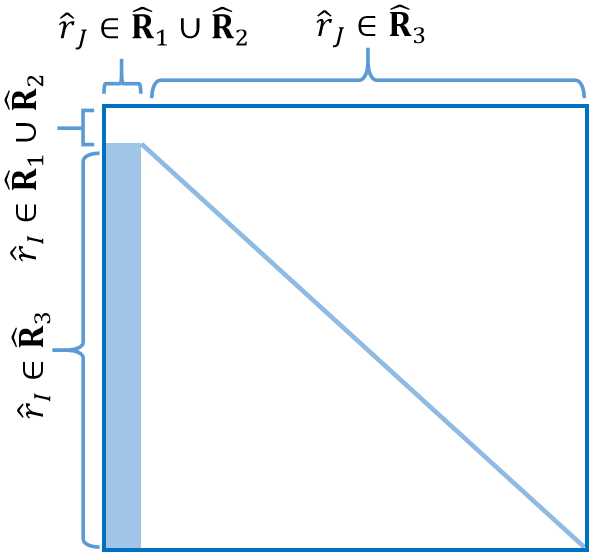
Figure 1: Matrix elements of $\bm{M}$ matrix required to be measured during the operator selection process are colored in blue.

3 Results and discussion

All the calculations are performed using the high-performance quantum emulating software Q²Chemistry ³³. The molecule orbitals and one- and two-electron integrals are evaluated using the PySCF ³⁴. The fermion-to-qubit mapping is executed through the Jordan-Wigner transformation using the OpenFermion ³⁵. All optimizations in the VQE method utilize the Broyden-Fletcher-Goldfarb-Shanno (BFGS) algorithm implemented in the SciPy ³⁶, with a convergence criteria of $\epsilon=10^{-3}$ for the norm of residual gradients. In the following, we indicate the qEOM-SDT methods before and after operator screening as qEOM-SDT and qEOM-SDt, respectively. A perturbation correction, as discussed in Section 2.3 (4), is further introduced to the qEOM-SDt, resulting in the method called qEOM-SD(t).

3.1 2 ${}^{1}\Delta$ excited state of $\rm CH^{+}$

The EOM-CCSD method performs poorly in predicting the second ${}^{1}\Delta$ excitation energy of $\rm CH^{+}$, with an energy error exceeding 3.5 eV. It is important to include the triple excitation operators in the EOM method to accurately describe this state ³⁷. The energy of the 2 ${}^{1}\Delta$ excited state is calculated at twice the equilibrium bond length ($2R_{e}=2\times 2.13713\enspace\rm{bohr}$) using the 6-31g basis set. $\rm CH^{+}$ possesses $C_{\infty v}$ symmetry, but in the calculations, a lower $C_{2v}$ symmetry is used.

The excitation energy deviations of qEOM-SDT, qEOM-SDt, qEOM-SD(t) and qEOM-SD with respect to the full configuration interaction (FCI) method are provided in Table 1. Analogous to the EOM-CCSD, for predicting the excitation energy of 2 ${}^{1}\Delta$, the qEOM-SD notably overestimates it by 3.90 eV. However, incorporating 82 (1.98%) triple excitation operators in qEOM-SDt reduces the errors by one orders of magnitude. As the number of retained operators increases, the errors of qEOM-SDt and qEOM-SD(t) approach that of qEOM-SDT, which is 0.11 eV. However, the rate of improvement in accuracy gradually slows down. The accuracy of qEOM-SD(t) consistently outperforms that of qEOM-SDt, but the difference between the two gradually diminishes. When $\epsilon_{t}=2.2\times 10^{-5}$, the number of operators in the $\hat{\mathbf{R}}=\hat{\mathbf{R}}_{1}\cup\hat{\mathbf{R}}_{2}\cup\hat{\mathbf{R}}_{3}$ and $\hat{\mathbf{R}}_{3}$, both before and after the operator screening are shown in Fig. 2. It demonstrates that the reduction in the number of operators based on symmetry exceeds 40% for $\hat{\mathbf{R}}$ and $\hat{\mathbf{R}}_{3}$, and similarly for perturbation, indicating significant effects for both approaches.

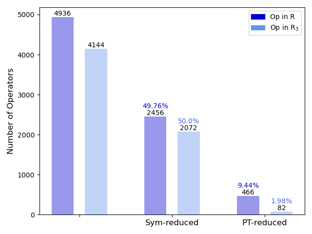
Figure 2: Reduction of the number of operators in the operator pool $\hat{\mathbf{R}}$ and $\hat{\mathbf{R}}_{3}$ for the qEOM-SD(t) method when $\epsilon_{t}=2.2\times 10^{-5}$.

Table 1: Energy deviations of the $2^{1}\Delta$ excited state computed with qEOM-SDt,qEOM-SD(t), qEOM-SDT and qEOM-SD methods for the CH⁺ molecule at twice the equilibrium bond length. The reference values are computed with the FCI method.

$\epsilon_{t}$	Op in $\hat{\mathbf{R}}_{3}$ after (before)	$\%$	$\Delta E_{\rm qEOM-SDt}$	$\Delta E_{\rm qEOM-SD(t)}$	$\Delta E_{\rm qEOM-SDT}$	$\Delta E_{\rm qEOM-SD}$
$2.2\times 10^{-5}$	82 (4144)	$1.98\%$	0.2004	0.1736	0.1075	3.9194
$3.0\times 10^{-6}$	182 (4144)	$4.39\%$	0.1278	0.1243
$2.55\times 10^{-7}$	282 (4144)	$6.81\%$	0.1196	0.1191

• The unit of energy difference is eV.

3.2 2 ${}^{1}\Sigma$ excited state of HF

An accurate description of the bond breaking for the HF molecule is a challenge task for traditional electronic structure methods. Here, we apply the qEOM methods to study the second ${}^{1}\Sigma$ state of the HF molecule at different bond lengths with the 6-31G basis, freezing the lowest molecular orbital. Although HF belongs to the $C_{\infty v}$ symmetry group, we use the lower $C_{2v}$ symmetry for convenience. In this symmetry, both the HF state and the 2 ${}^{1}\Sigma$ excited state belong to the $A_{1}$ irrep.

Fig. 3 shows the energy differences as a function of the H-F bond length $R_{\rm H-F}$ between the qEOM-SDT, qEOM-SDt, qEOM-SD(t) and qEOM-SD methods compared to complete active space configuration interaction (CASCI). The results indicate that the qEOM-SDt and qEOM-SD(t) methods are sufficiently accurate compared to the exact diagonalization method CASCI. The qEOM-SD method fails to accurately capture the electron correlation of the 2 ${}^{1}\Sigma$ state at the large bond length. Specifically, when $R_{\rm H-F}=5$ bohr, the error exceeds 0.9 eV. In contrast, the qEOM-SDt and qEOM-SD(t) methods exhibit much smaller errors of approximately 0.07 eV and 0.06 eV, respectively.

Table 2 illustrates that the qEOM-SDt and qEOM-SD(t) methods, using a maximum of only 61 (1.36%) triple excitation operators, accurately recover the correlation energy in the 2 ${}^{1}\Sigma$ excited state, with average errors of 0.03 eV and 0.01 eV, respectively. Additionally, when $R_{\rm H-F}=1.5$ and $2.1$ bohr the qEOM-SD(t) results outperform qEOM-SDT. However, as the threshold $\epsilon_{t}$ increases, the precision of qEOM-SD(t) and EOM-SDt will gradually approach that of qEOM-SDT. While other methods tend to overestimate the excitation energy, qEOM-SD(t) underestimates it when $R_{\rm H-F}=6.0$ bohr. Generally, qEOM-SD(t) yields better results than qEOM-SDt. Note that the excitation state accuracy obtained from qEOM-SDt and qEOM-SD(t) calculations based on VQE may surpass the ground state accuracy obtained from VQE calculations. Similar findings are also mentioned in Ref. ²⁶ for qEOM-SD.

Table 2: Energy deviations of the $2^{1}\Sigma$ excited state computed with qEOM-SDt, qEOM-SD(t), qEOM-SDT and qEOM-SD methods for the HF molecule at different bond lengths. The reference values are computed with the CASCI method.

$R_{\rm H-F}$	Op in $\hat{\mathbf{R}}_{3}$ after(before)	$\%$	$\Delta E_{\rm qEOM-SDt}$	$\Delta E_{\rm qEOM-SD(t)}$	$\Delta E_{\rm qEOM-SDT}$	$\Delta E_{\rm qEOM-SD}$
1.5	40 (4480)	0.89%	0.0324	0.0019	0.0067	0.1089
2.1	48 (4480)	1.07%	0.0345	0.0079	0.0103	0.1280
2.7	61 (4480)	1.36%	0.0337	0.0110	0.0100	0.3837
3.2	43 (4480)	0.96%	0.0314	0.0141	0.0110	0.4938
3.7	38 (4480)	0.85%	0.0319	0.0056	0.0052	0.1110
4.2	33 (4480)	0.74%	0.0272	0.0061	0.0049	0.2997
5.0	45 (4480)	1.00%	0.0698	0.0552	0.0255	0.9022
6.0	30 (4480)	0.67%	0.0119	-0.0028	0.0000	0.0981
$\overline{x}$	42.25	0.94%	0.0341	0.012375	0.0092	0.3157
$\sigma$	9.02	0.20%	0.0151	0.0169	0.0070	0.2617

• The unit of excitation energy deviations are in eV, and bond length is in bohr.

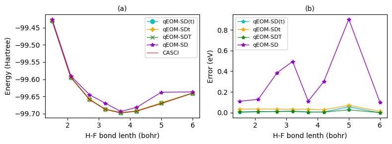
Figure 3: (a) Potential energy surfaces (b) energy error as a function of the H-F bond length computed using CASCI, qEOM-SD, qEOM-SDt, qEOM-SD(t) and qEOM-SDT methods.

3.3 2 ${}^{1}Ag$ excited state of $\rm H_{8}$

It is well known that the EOM-CCSD method is able to treat the excited states dominated by single electron excitation while its accuracy rapidly deteriorates when double electron excitations are involved. The second ${}^{1}Ag$ state of the $\rm H_{8}$ system is dominated by the biexcited $2\,a_{g}^{2}\rightarrow 1\,b_{1g}^{2}$ configuration, posing a great challenge for the EOM-CCSD and qEOM-SD methods. ³⁸ The structure of the $\rm H_{8}$ is depicted in Fig. 4, with its stretching distance from the regular octahedron denoted as $b$.

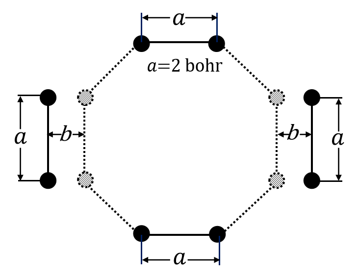
Figure 4: Structure of the $\rm{H_{8}}$ system.

The basis set for the hydrogen atom comprises three primitive Gaussian-type functions (S-type), with exponents of 4.50038, 0.681277, and 0.151374, and corresponding contraction coefficients of 0.07048, 0.40789, and 0.64767, respectively. ³⁹ The highest point symmetry $D_{2h}$ is used to reduce the number of operators in $\hat{\mathbf{R}}$.

Table 3: Energy deviations of the 2 ${}^{1}Ag$ excited state computed with qEOM-SDt, qEOM-SD(t), qEOM-SDT and qEOM-SD methods for the $\rm H_{8}$ system at different $b$. The reference values are computed with the CASCI method.

$b$	Op in $\hat{\mathbf{R}}_{3}$ after (before)	%	$\Delta E_{\rm qEOM-SDt}$	$\Delta E_{\rm qEOM-SD(t)}$	$\Delta E_{\rm qEOM-SDT}$	$\Delta E_{\rm qEOM-SD}$
1.0	96 (1184)	$8.11\%$	0.1456	0.1326	0.0586	0.6989
0.8	88 (1184)	$7.43\%$	0.1468	0.1347	0.0649	0.8357
0.6	90 (1184)	$7.60\%$	0.1465	0.1377	0.0813	0.9336
0.4	86 (1184)	$7.26\%$	0.1575	0.1493	0.1038	1.0000
0.2	84 (1184)	$7.09\%$	0.1757	0.1681	0.1310	0.9994
$\overline{x}$	88.80	7.50%	0.1544	0.1445	0.0879	0.8935
$\sigma$	4.12	0.35%	0.0115	0.0131	0.0266	0.1143

• The unit of excitation energy deviations are in eV, and $b$ is in bohr.

Table 3 shows the energy deviations of the 2 ${}^{1}Ag$ excited state computed with qEOM-SD(t), qEOM-SDt, qEOM-SDT and qEOM-SD methods for the $\rm H_{8}$ system, which generally exhibit an increasing trend as $b$ decreases. The average energy deviation of qEOM-SD is about 0.89 eV for $b$ ranging from 1.0 to 0.2 bohr. However, for qEOM-SDt and qEOM-SD(t) methods, it is nearly 0.15 eV. In contrast with 2 ${}^{1}\Sigma$ excited state of HF and 2 ${}^{1}\Delta$ excited state of $\rm CH^{+}$, more triple excitation operators up to an average of 7.50% are involved in the qEOM-SDt and qEOM-SD(t) calculations.

4 Quantum Subspace Expansion with single, double, and triple excitations

Both the QSE and qEOM methods have been suggested for calculating molecular excitation energies. These two methods also share some similar features in the subspace expansion and formulation of the working equation. Here, we extend the operator screening technique to the QSE to include the triple excitations.

4.1 QSE-SDT method

In the QSE method, the generalized eigenvalue equation is written as

$$\bm{HD}_{m}=E_{m}\bm{SD}_{m}$$ (34)

where $\bm{S}$ is the overlap matrix. The elements of $\bm{S}$ and $\bm{H}$ are defined as

$$\begin{split}\bm{S}_{IJ}&=\langle\psi_{0}|\hat{r}_{I}^{{\dagger}}\hat{r}_{J}|\psi_{0}\rangle\\ \bm{H}_{IJ}&=\langle\psi_{0}|\hat{r}_{I}^{{\dagger}}\hat{H}\hat{r}_{J}|\psi_{0}\rangle\end{split}$$ (35)

In contrast to the qEOM method, the QSE method does not ensure the orthogonality among the subspace basis $\{\hat{r}_{I}\hat{U}|{\psi_{\rm HF}}\rangle|\hat{r}_{I}\in\hat{\mathbf{R}}\}$, so the ground state $|{\psi_{0}}\rangle$ should be included in the subspace expansion.

As discussed in Section 2.3, the working equation of QSE can also be block diagonalized, that is

$${\rm Irrep}(\hat{r}_{I}|{\psi_{0}\rangle})=\rm Irrep(|\psi_{m}\rangle)$$

Additionally, one can use the perturbation theory to further reduce the number of triple excitation operators in $\hat{\mathbf{R}}$ per irreducible representation. Like the qEOM, it is able to define the zero- and first-order wave function using $\hat{\mathbf{R}}_{1}\cup\hat{\mathbf{R}}_{2}$ and $\hat{\mathbf{R}}_{3}$ respectively as

$$\begin{split}{|\psi_{m}^{(0)}\rangle}=\sum_{\begin{subarray}{c}\hat{r}_{I}\in{\hat{\mathbf{R}}_{1}\cup\hat{\mathbf{R}}_{2}}\end{subarray}}\gamma_{I}\hat{r}_{I}|\psi_{0}\rangle\\ {|\psi_{m}^{(1)}\rangle}=\sum_{\begin{subarray}{c}\hat{r}_{I}\in{\hat{\mathbf{R}}_{3}}\end{subarray}}\gamma_{I}\hat{r}_{I}|\psi_{0}\rangle.\end{split}$$ (36)

As such, the weight coefficients can be formulated following the derivation presented in Section 2.3 as

$$W_{I}=\frac{|\langle\psi_{\rm 0}|r_{I}^{\dagger}\hat{H}|\psi_{m}^{(0)}\rangle-E_{m}^{(0)}\langle\psi_{\rm 0}|r_{I}^{\dagger}|\psi_{m}^{(0)}\rangle|^{2}}{E_{m}^{(0)}\langle\psi_{\rm 0}|r_{I}^{\dagger}\hat{r}_{I}|\psi_{\rm 0}\rangle-\langle\psi_{\rm 0}|r_{I}^{\dagger}\hat{H}\hat{r}_{I}|\psi_{\rm 0}\rangle}$$ (37)

Finally, the perturbation correction is performed as in Section 2.3 (4).

4.2 2 ${}^{1}Ag$ excited state of $\rm H_{8}$

Table 4 shows the energy deviations of the 2 ${}^{1}Ag$ excited state computed with QSE-SDt, QSE-SD(t), QSE-SDT and QSE-SD methods for the $\rm H_{8}$ system. To facilitate comparison with the qEOM method, the basis set, molecular information, and the number of selected operators for each bond length are the same as those used in the qEOM calculations. The average energy deviations of QSE-SDt, QSE-SD(t), QSE-SDT and QSE-SD are about 0.15 eV, 0.14 eV, 0.09 eV and 0.89 eV. The overall performance of the QSE and qEOM methods is very similar. However, the QSE offers an improvement in accuracy by an order of magnitude of $10^{-3}$ compared to the qEOM method.

Table 4: Energy deviations of the 2 ${}^{1}Ag$ excited state computed with QSE-SDt, QSE-SD(t), QSE-SDT and QSE-SD methods for the $\rm H_{8}$ system at different $b$. The reference values are computed with the CASCI method.

$b$	Op in $\hat{\mathbf{R}}_{3}$ after (before)	$\%$	$\Delta E_{\rm QSE-SDt}$	$\Delta E_{\rm QSE-SD(t)}$	$\Delta E_{\rm QSE-SDT}$	$\Delta E_{\rm QSE-SD}$
1.0	96 (1184)	$8.11\%$	0.1336	0.1235	0.0462	0.6833
0.8	88 (1184)	$7.43\%$	0.1446	0.1341	0.0641	0.8331
0.6	90 (1184)	$7.60\%$	0.1464	0.1381	0.0816	0.9307
0.4	86 (1184)	$7.26\%$	0.1560	0.1484	0.1023	0.9935
0.2	84 (1184)	$7.09\%$	0.1799	0.1732	0.1333	0.9899
$\overline{x}$	88.8	$7.50\%$	0.1521	0.14346	0.0855	0.8861
$\sigma$	4.1	$0.35\%$	0.0156	0.0169	0.0303	0.1168

• The units of energy and energy difference are eV and $b$ is in bohr.

5 Conclusion and outlook

In this work, we numerically demonstrate that the qEOM-SD method is unable to accurately describe molecule excitation energies dominated by double and high-order excitations, which commonly exist in the excited states of (near-) degenerate systems. In order to overcome this issue, we propose the qEOM-SDT method to improve the accuracy of the qEOM thoery by including the triple excitations. Numerical calculations of excitation energies for small molecular systems, including CH^†, HF and H₈, demonstrates the qEOM-SDT method reduces the energe errors by one to two order of magnitude, in contrast to the qEOM-SD method.

In order to reduce the computational complexity of qEOM-SDT, we propose a method called qEOM-SDt, which utilizes point group symmetry and perturbation theory to reduce the number of triple excitation operators in qEOM-SDT calculations. We further introduce qEOM-SD(t), where the energy corrections from the unselected triple excitation operators are replaced by their associated first-order perturbation energies. Numerical results show that qEOM-SD(t) generally provides better excitation state accuracy than qEOM-SDt. However, unlike qEOM-SDt and qEOM-SDT, it may underestimate excitation energies. Both methods can provide satisfactory excitation energies with few triple excitation operators, and in some cases, the excitation energy accuracy is higher than the ground state accuracy obtained from VQE calculations. The computational bottleneck of the qEOM-SDT mainly results from estimating the weight coefficients used for the operator screening instead of measuring all Hamiltonian matrix elements involving triple excitation operators in the qEOM-SDT. The same operator reduction procedure is also extended to the QSE for calculating excitation energies. The new algorithms presented in this work provide a promising tool for studying electronically excited states on a quantum computer.

6 Acknowledgments

This work was supported by Innovation Program for Quantum Science and Technology (2021ZD0303306), the National Natural Science Foundation of China (22073086, 22288201), Anhui Initiative in Quantum Information Technologies (AHY090400), and the Fundamental Research Funds for the Central Universities (WK2060000018).

7 Appendix

In the following, we will show the derivation of the criterion of operator selection in ADAPT-VQE ansatz with UCC operator pool. This mainly follows the derivation of the criterion of operator selection in ADAPT-VQE ansatz showed in ³¹.

The point group $G$ of the system is Abelian, and $\hat{R}_{i}$ is an symmetry operation in it. So, we have $\hat{R}_{i}^{{\dagger}}\hat{H}\hat{R}_{i}=\hat{H}$, and

$$\hat{H}\hat{R}_{i}|\psi_{0}\rangle=\hat{R}_{i}\hat{H}|\psi_{0}\rangle=E_{0}\hat{R}_{i}|\psi_{0}\rangle$$ (38)

If the ground state is nondegenerate, $\hat{R}_{i}|\psi_{0}\rangle$ and $|\psi_{0}\rangle$ is the same state but can differ by a coefficient, i.e.,

$$\hat{R}_{i}|\psi_{0}\rangle=\lambda|\psi_{0}\rangle$$ (39)

Thus, $|\psi_{0}\rangle$ forms an one-dimensional invariant subspace under the point group $G$, and in this subspace the irreducible character correspond to $\hat{R}_{i}$ is $\lambda$. The HF state also forms an invariant subspace, and its irreducible character for $\hat{R}_{i}$ is termed as $\beta$.

$$\hat{R}_{i}|\psi_{\rm{HF}}\rangle=\beta|\psi_{\rm{HF}}\rangle$$ (40)

Since $\hat{R}_{i}^{{\dagger}}\hat{R}_{i}=\hat{I}$, we have

$$\langle\psi_{\rm{HF}}|\psi_{0}\rangle=\langle\psi_{\rm{HF}}|\hat{R}_{i}^{{\dagger}}\hat{R}_{i}|\psi_{0}\rangle=\lambda\beta\langle\psi_{\rm{HF}}|\psi_{0}\rangle$$ (41)

So, $\lambda\beta=1$. And for the Abelian group, the characters are 1 or -1. Therefore, $\lambda=\beta$, which means $\psi_{\rm{HF}}$ and $\psi_{0}$ belong to the same irreducible representation (irrep).

$$\rm{Irrep}(\psi_{\rm{HF}})=\rm{Irrep}(\psi_{0})$$ (42)

The ground state calculated by ADAPT-VQE ansatz

$$|\psi_{\rm{VQE}}\rangle=\prod\limits_{i=0}\left(e^{\theta_{i}\left(\hat{T}_{i}-\hat{T}_{i}^{{\dagger}}\right)}\right)|\psi_{\rm HF}\rangle$$ (43)

should satisfy the above condition. Based on Taylor expansion and $\hat{T}_{i}^{{\dagger}}\psi_{\rm{HF}}=0$, we have

$$\begin{split}|\psi_{\rm{VQE}}\rangle&=\prod\limits_{i=0}\left(1+\theta_{i}(\hat{T}_{i}-\hat{T}_{i}^{{\dagger}})+\frac{\theta_{i}^{2}}{2}(\hat{T}_{i}-\hat{T}_{i}^{{\dagger}})^{2}+\cdots\right)|\psi_{\rm HF}\rangle\\ &=c_{0}|\psi_{\rm{HF}}\rangle+\sum_{i}c_{i}T_{i}|\psi_{\rm{HF}}\rangle+\sum_{i}c_{i}T_{i}^{2}|\psi_{\rm{HF}}\rangle+\cdots\end{split}$$ (44)

Since $\psi_{\rm{HF}}$ and $\psi_{0}$ belong to the same irrep, every term in the above equation should belong to the same irrep of $\psi_{\rm{HF}}$, i.e.,

$${\rm{Irrep}}(T_{i}\psi_{\rm{HF}})=\rm{Irrep}(\psi_{0})$$ (45)

References

- Pulay 2011 Pulay, P. A perspective on the CASPT2 method. Int. J. Quantum Chem. 2011, 111, 3273–3279
- Szalay et al. 2012 Szalay, P. G.; Müller, T.; Gidofalvi, G.; Lischka, H.; Shepard, R. Multiconfiguration Self-Consistent Field and Multireference Configuration Interaction Methods and Applications. Chem. Rev. 2012, 112, 108–181
- Baiardi et al. 2022 Baiardi, A.; Kelemen, A. K.; Reiher, M. Excited-State DMRG Made Simple with FEAST. J. Chem. Theory Comput. 2022, 18, 415–430
- Schriber and Evangelista 2017 Schriber, J. B.; Evangelista, F. A. Adaptive Configuration Interaction for Computing Challenging Electronic Excited States with Tunable Accuracy. J. Chem. Theory Comput. 2017, 13, 5354–5366
- Aspuru-Guzik et al. 2005 Aspuru-Guzik, A.; Dutoi, A. D.; Love, P. J.; Head-Gordon, M. Simulated quantum computation of molecular energies. Science 2005, 309, 1704–1707
- Peruzzo et al. 2014 Peruzzo, A.; McClean, J.; Shadbolt, P.; Yung, M.-H.; Zhou, X.-Q.; Love, P. J.; Aspuru-Guzik, A.; O’brien, J. L. A variational eigenvalue solver on a photonic quantum processor. Nature communications 2014, 5, 4213
- McArdle et al. 2020 McArdle, S.; Endo, S.; Aspuru-Guzik, A.; Benjamin, S. C.; Yuan, X. Quantum computational chemistry. Reviews of Modern Physics 2020, 92, 015003
- Su et al. 2021 Su, Y.; Berry, D. W.; Wiebe, N.; Rubin, N.; Babbush, R. Fault-tolerant quantum simulations of chemistry in first quantization. PRX Quantum 2021, 2, 040332
- O’Malley et al. 2016 O’Malley, P. J.; Babbush, R.; Kivlichan, I. D.; Romero, J.; McClean, J. R.; Barends, R.; Kelly, J.; Roushan, P.; Tranter, A.; Ding, N.; others Scalable quantum simulation of molecular energies. Physical Review X 2016, 6, 031007
- Parrish et al. 2019 Parrish, R. M.; Hohenstein, E. G.; McMahon, P. L.; Martínez, T. J. Quantum computation of electronic transitions using a variational quantum eigensolver. Physical review letters 2019, 122, 230401
- Nakanishi et al. 2019 Nakanishi, K. M.; Mitarai, K.; Fujii, K. Subspace-search variational quantum eigensolver for excited states. Physical Review Research 2019, 1, 033062
- Ryabinkin et al. 2018 Ryabinkin, I. G.; Genin, S. N.; Izmaylov, A. F. Constrained variational quantum eigensolver: Quantum computer search engine in the Fock space. Journal of chemical theory and computation 2018, 15, 249–255
- Stair et al. 2020 Stair, N. H.; Huang, R.; Evangelista, F. A. A multireference quantum Krylov algorithm for strongly correlated electrons. J. Chem. Theory Comput. 2020, 16, 2236–2245
- Jones et al. 2019 Jones, T.; Endo, S.; McArdle, S.; Yuan, X.; Benjamin, S. C. Variational quantum algorithms for discovering Hamiltonian spectra. Physical Review A 2019, 99, 062304
- Tilly et al. 2020 Tilly, J.; Jones, G.; Chen, H.; Wossnig, L.; Grant, E. Computation of molecular excited states on IBM quantum computers using a discriminative variational quantum eigensolver. Physical Review A 2020, 102, 062425
- Bauman et al. 2021 Bauman, N. P.; Liu, H.; Bylaska, E. J.; Krishnamoorthy, S.; Low, G. H.; Granade, C. E.; Wiebe, N.; Baker, N. A.; Peng, B.; Roetteler, M.; Troyer, M.; Kowalski, K. Toward Quantum Computing for High-Energy Excited States in Molecular Systems: Quantum Phase Estimations of Core-Level States. J. Chem. Theory Comput. 2021, 17, 201–210
- Kang et al. 2022 Kang, C.; Bauman, N. P.; Krishnamoorthy, S.; Kowalski, K. Optimized Quantum Phase Estimation for Simulating Electronic States in Various Energy Regimes. J. Chem. Theory Comput. 2022, 18, 6567–6576
- Baker 2021 Baker, T. E. Lanczos recursion on a quantum computer for the Green’s function and ground state. Physical Review A 2021, 103, 032404
- Preskill 2018 Preskill, J. Quantum computing in the NISQ era and beyond. Quantum 2018, 2, 79
- Sharma et al. 2020 Sharma, K.; Khatri, S.; Cerezo, M.; Coles, P. J. Noise resilience of variational quantum compiling. New Journal of Physics 2020, 22, 043006 (29pp)
- Chan et al. 2021 Chan, H. H. S.; Fitzpatrick, N.; Segarra-Martí, J.; Bearpark, M. J.; Tew, D. P. Molecular excited state calculations with adaptive wavefunctions on a quantum eigensolver emulation: reducing circuit depth and separating spin states. Physical Chemistry Chemical Physics 2021, 23, 26438–26450
- Higgott et al. 2019 Higgott, O.; Wang, D.; Brierley, S. Variational quantum computation of excited states. Quantum 2019, 3, 156
- Santagati et al. 2018 Santagati, R.; Wang, J.; Gentile, A. A.; Paesani, S.; Wiebe, N.; McClean, J. R.; Morley-Short, S.; Shadbolt, P. J.; Bonneau, D.; Silverstone, J. W.; others Witnessing eigenstates for quantum simulation of Hamiltonian spectra. Science advances 2018, 4, eaap9646
- Lee et al. 2018 Lee, J.; Huggins, W. J.; Head-Gordon, M.; Whaley, K. B. Generalized unitary coupled cluster wave functions for quantum computation. J. Chem. Theory Comput. 2018, 15, 311–324
- McClean et al. 2017 McClean, J. R.; Kimchi-Schwartz, M. E.; Carter, J.; De Jong, W. A. Hybrid quantum-classical hierarchy for mitigation of decoherence and determination of excited states. Physical Review A 2017, 95, 042308
- Ollitrault et al. 2020 Ollitrault, P. J.; Kandala, A.; Chen, C.-F.; Barkoutsos, P. K.; Mezzacapo, A.; Pistoia, M.; Sheldon, S.; Woerner, S.; Gambetta, J. M.; Tavernelli, I. Quantum equation of motion for computing molecular excitation energies on a noisy quantum processor. Physical Review Research 2020, 2, 043140
- Asthana et al. 2023 Asthana, A.; Kumar, A.; Abraham, V.; Grimsley, H.; Zhang, Y.; Cincio, L.; Tretiak, S.; Dub, P. A.; Economou, S. E.; Barnes, E.; others Quantum self-consistent equation-of-motion method for computing molecular excitation energies, ionization potentials, and electron affinities on a quantum computer. Chemical Science 2023, 14, 2405–2418
- Piecuch et al. 2004 Piecuch, P.; Kowalski, K.; Pimienta, I.; Fan, P.-D.; Lodriguito, M.; McGuire, M.; Kucharski, S.; Kuś, T.; Musiał, M. Method of moments of coupled-cluster equations: a new formalism for designing accurate electronic structure methods for ground and excited states. Theoretical Chemistry Accounts 2004, 112, 349–393
- Włoch et al. 2005 Włoch, M.; Gour, J. R.; Kowalski, K.; Piecuch, P. Extension of renormalized coupled-cluster methods including triple excitations to excited electronic states of open-shell molecules. The Journal of chemical physics 2005, 122
- Grimsley et al. 2019 Grimsley, H. R.; Economou, S. E.; Barnes, E.; Mayhall, N. J. An adaptive variational algorithm for exact molecular simulations on a quantum computer. Nature communications 2019, 10, 3007
- Cao et al. 2022 Cao, C.; Hu, J.; Zhang, W.; Xu, X.; Chen, D.; Yu, F.; Li, J.; Hu, H.-S.; Lv, D.; Yung, M.-H. Progress toward larger molecular simulation on a quantum computer: Simulating a system with up to 28 qubits accelerated by point-group symmetry. Physical Review A 2022, 105, 062452
- Cotton 1991 Cotton, F. A. Chemical applications of group theory; John Wiley & Sons, 1991
- Fan et al. 2022 Fan, Y.; Liu, J.; Zeng, X.; Xu, Z.; Shang, H.; Li, Z.; Yang, J. Q¡sup¿2¡/sup¿Chemistry: A quantum computation platform for quantum chemistry. JUSTC 2022, 52, 2
- Sun et al. 2018 Sun, Q.; Berkelbach, T. C.; Blunt, N. S.; Booth, G. H.; Guo, S.; Li, Z.; Liu, J.; McClain, J. D.; Sayfutyarova, E. R.; Sharma, S.; others PySCF: the Python-based simulations of chemistry framework. Wiley Interdisciplinary Reviews: Computational Molecular Science 2018, 8, e1340
- McClean et al. 2020 McClean, J. R.; Rubin, N. C.; Sung, K. J.; Kivlichan, I. D.; Bonet-Monroig, X.; Cao, Y.; Dai, C.; Fried, E. S.; Gidney, C.; Gimby, B.; others OpenFermion: the electronic structure package for quantum computers. Quantum Science and Technology 2020, 5, 034014
- Virtanen et al. 2020 Virtanen, P.; Gommers, R.; Oliphant, T. E.; Haberland, M.; Reddy, T.; Cournapeau, D.; Burovski, E.; Peterson, P.; Weckesser, W.; Bright, J.; others SciPy 1.0: fundamental algorithms for scientific computing in Python. Nature methods 2020, 17, 261–272
- Kowalski and Piecuch 2004 Kowalski, K.; Piecuch, P. New coupled-cluster methods with singles, doubles, and noniterative triples for high accuracy calculations of excited electronic states. J. Chem. Phys. 2004, 120, 1715–1738
- Kowalski and Piecuch 2001 Kowalski, K.; Piecuch, P. The active-space equation-of-motion coupled-cluster methods for excited electronic states: Full EOMCCSDt. The Journal of Chemical Physics 2001, 115, 643–651
- Jankowski et al. 1985 Jankowski, K.; Meissner, L.; Wasilewski, J. Davidson-type corrections for quasidegenerate states. International journal of quantum chemistry 1985, 28, 931–942