Variational Analysis in the Wasserstein Space

Abstract

We study optimization problems whereby the optimization variable is a probability measure. Since the probability space is not a vector space, many classical and powerful methods for optimization (e.g., gradients) are of little help. Thus, one typically resorts to the abstract machinery of infinite-dimensional analysis or other ad-hoc methodologies, not tailored to the probability space, which however involve projections or rely on convexity-type assumptions. We believe instead that these problems call for a comprehensive methodological framework for calculus in probability spaces. In this work, we combine ideas from optimal transport, variational analysis, and Wasserstein gradient flows to equip the Wasserstein space (i.e., the space of probability measures endowed with the Wasserstein distance) with a variational structure, both by combining and extending existing results and introducing novel tools. Our theoretical analysis culminates in very general necessary optimality conditions for optimality. Notably, our conditions (i) resemble the rationales of Euclidean spaces, such as the Karush-Kuhn-Tucker and Lagrange conditions, (ii) are intuitive, informative, and easy to study, and (iii) yield closed-form solutions or can be used to design computationally attractive algorithms. We believe this framework lays the foundation for new algorithmic and theoretical advancements in the study of optimization problems in probability spaces, which we exemplify with numerous case studies and applications to machine learning, drug discovery, and distributionally robust optimization.

^∗ Equal contribution. This research was supported by the Swiss National Science Foundation under the NCCR Automation, grant agreement 51NF40_180545.

1 Main result

This work considers optimization problems of the form

$$\inf_{\operatorname{\mu}\in\operatorname{\mathcal{C}}}\,\operatorname{\mathcal{J}}(\operatorname{\mu}),$$ (1)

where $\operatorname{\mathcal{C}}\subseteq\mathcal{P}(\mathbb{R}^{d})$ is a set of admissible probability measures and $\operatorname{\mathcal{J}}:\mathcal{P}(\mathbb{R}^{d})\to\bar{\mathbb{R}}$ is a functional to minimize. This abstract problem setting stems from the observation that numerous fields, including machine learning, robust optimization, and biology, tackle their own version of (1), but with ad-hoc methods that often cease to be effective as soon as the problem structure deviates from idealized assumptions. Despite the recent efforts in the literature [1], these problems still demand a comprehensive theory for the optimization problem (1), which is the subject of this work. Specifically, we derive novel necessary first-order optimality conditions for (1), for arbitrary functionals and constraints. These formally resemble the rationales of Euclidean spaces (e.g., Karush–Kuhn–Tucker and Lagrange conditions) and are intuitive, informative, and easy to study. As a byproduct of our analysis, we translate tools from variational analysis (e.g., generalized subgradients, normal cones, tangent cones, etc.) to the Wasserstein space (i.e., the probability space endowed with the Wasserstein distance). After practicing these novel tools in numerous pedagogical examples, we tackle open problems arising in machine learning, drug discovery, and distributionally robust optimization (DRO), showcasing how our conditions result either in closed-form solutions of (1) or computationally attractive algorithms.

Our main result are general first-order optimality conditions of (1):

[First-order optimality conditions] If $\operatorname{\mu^{\ast}}\in\mathcal{P}(\mathbb{R}^{d})$ is an optimal solution of (1) with finite second moment and provided that a constraint qualification holds, then the “Wasserstein subgradients” are “aligned” with the constraints at “optimality”, i.e.,

$$\mathbf{0}_{\operatorname{\mu^{\ast}}}\in\partial\operatorname{\mathcal{J}}(\operatorname{\mu^{\ast}})+\operatorname{N}_{\operatorname{\mathcal{C}}}(\operatorname{\mu^{\ast}}),$$

where $\partial\operatorname{\mathcal{J}}(\operatorname{\mu^{\ast}})$ is the “Wasserstein subgradient” of $\operatorname{\mathcal{J}}$ at $\operatorname{\mu^{\ast}}$, $\operatorname{N}_{\operatorname{\mathcal{C}}}(\operatorname{\mu^{\ast}})$ is the “Wasserstein normal cone” of $\operatorname{\mathcal{C}}$ at $\operatorname{\mu^{\ast}}$ and $\mathbf{0}_{\operatorname{\mu^{\ast}}}$ is a “null Wasserstein tangent vector” at $\operatorname{\mu^{\ast}}$.

As corollaries of our theorem, we obtain the “Wasserstein counterparts” of Fermat’s rule in the unconstrained setting (i.e., the gradient vanishes at optimality) and the Lagrange conditions for (in)equality-constrained settings (i.e., the “gradients” of the objective and the constraint are “aligned” at “optimality”, see Figure 1).

Before diving into variational analysis in the Wasserstein space, we illustrate our optimality conditions by informally studying a simple and accessible version of (1). For $\theta\neq 0$ and $\varepsilon>0$, consider the problem

$$\inf_{\operatorname{\mu}\in\mathcal{P}_{2}(\mathbb{R}^{d})}\;\mathbb{E}^{x\sim\operatorname{\mu}}\left[\left\langle\theta,x\right\rangle\right]\qquad\text{subject to}\qquad\mathbb{E}^{x\sim\operatorname{\mu}}\left[\left\|x\right\|^{2}\right]\leq\varepsilon^{2},$$ (2)

depicted in Figure 1 for $\theta=\begin{bmatrix}1&1\end{bmatrix}^{\top}$. To get some intuition, let us restrict to Dirac’s delta of the form $\delta_{x}$ for $x\in\mathbb{R}^{d}$. Accordingly, (2) reduces to $\inf_{\left\|x\right\|^{2}\leq\varepsilon^{2}}\left\langle\theta,x\right\rangle.$ This optimization problem can be studied through standard first-order optimality conditions in Euclidean spaces. Since the gradient of the objective $\nabla_{x}{\left\langle\theta,x\right\rangle}=\theta$ never vanishes, the optimal solution (if it exists) lies at the boundary. We thus seek the Lagrange multiplier $\lambda>0$ such that

$$0=\nabla_{x}{\left\langle\theta,x\right\rangle}+\lambda\nabla_{x}{\left\|x\right\|^{2}}=\theta+2\lambda x\quad\text{and}\quad\varepsilon^{2}=\left\|x\right\|^{2},$$ (3)

which yields $x=-\varepsilon\frac{\theta}{\left\|\theta\right\|}$ and $\lambda=\frac{\left\|\theta\right\|}{2\varepsilon}$. Now back to (2): After basic algebraic manipulations, our main result (stated informally above) tells us that any solution $\operatorname{\mu^{\ast}}\in\mathcal{P}_{2}(\mathbb{R}^{d})$ of (2) satisfies the Lagrange-like condition

$$0=2\lambda x+\theta\quad\operatorname{\mu^{\ast}}-\text{a.e.}\quad\text{and}\quad\varepsilon^{2}=\mathbb{E}^{x\sim\operatorname{\mu^{\ast}}}\left[\left\|x\right\|^{2}\right]=\frac{\left\|\theta\right\|^{2}}{4\lambda^{2}},$$ (4)

for some $\lambda\geq 0$ constant across the support of $\operatorname{\mu^{\ast}}$; cf. Figure 1 for $\theta=\begin{bmatrix}1&1\end{bmatrix}^{\top}$. We conclude that the mass of any candidate solution is necessarily located at $-\varepsilon\frac{\theta}{\left\|\theta\right\|}$. In particular, our optimality condition in (4) mirrors its counterpart on $\mathbb{R}^{d}$ in (3).

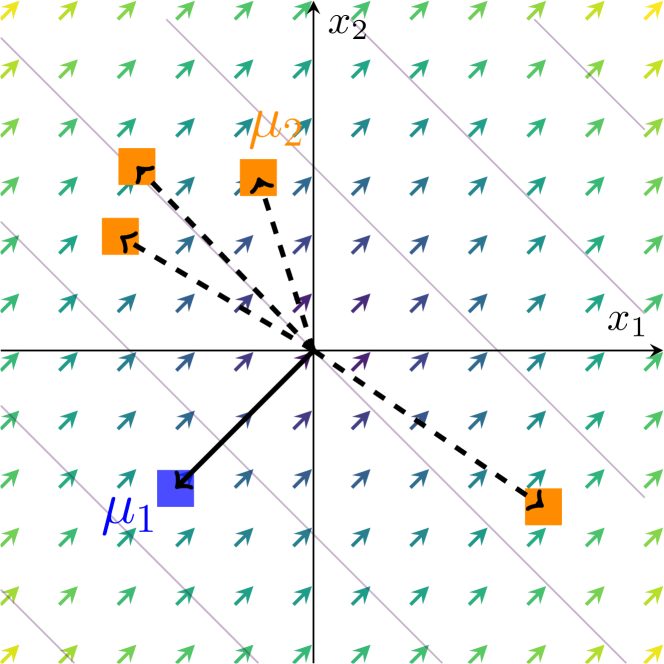
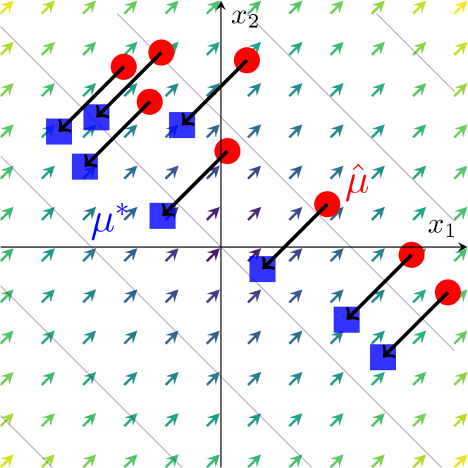
Figure 1: “Gradients” are “aligned” with the constraints at “optimality”. The figure on the left depicts two empirical candidate solutions ${\color[rgb]{0,0,1}\operatorname{\mu}_{1}}$ and ${\color[rgb]{1,0.55078125,0}\operatorname{\mu}_{2}}$ for (1) with $\operatorname{\mathcal{C}}=\{\operatorname{\mu}\in\mathcal{P}_{2}(\mathbb{R}^{2})\,|\,\mathbb{E}^{(x_{1},x_{2})\sim\operatorname{\mu}}\left[x_{1}^{2}+x_{2}^{2}\right]\leq\varepsilon^{2}\}$ (i.e., bounded second moment) and $\operatorname{\mathcal{J}}(\operatorname{\mu})=\mathbb{E}^{(x_{1},x_{2})\sim{\color[rgb]{0,0,1}\operatorname{\mu}}}\left[x_{1}+x_{2}\right]$, of which we show the contours and the gradient vector field. The solid (resp., dashed) black arrows represent the gradient of the constraint function $\mathbb{E}^{(x_{1},x_{2})\sim\operatorname{\mu}}\left[x_{1}^{2}+x_{2}^{2}\right]-\varepsilon^{2}$ at ${\color[rgb]{0,0,1}\operatorname{\mu}_{1}}$ (resp., ${\color[rgb]{1,0.55078125,0}\operatorname{\mu}_{2}}$). Here, ${\color[rgb]{0,0,1}\operatorname{\mu}_{1}}$ is indeed a candidate optimal solution: The gradient of the objective is aligned with the gradient of the constraint. For ${\color[rgb]{1,0.55078125,0}\operatorname{\mu}_{2}}$, instead, these two are not aligned. Thus, ${\color[rgb]{1,0.55078125,0}\operatorname{\mu}_{2}}$ cannot be optimal. The figure on the right shows that ${\color[rgb]{0,0,1}\operatorname{\mu^{\ast}}}$ satisfies the optimality condition for (1) with $\operatorname{\mathcal{C}}=\bar{\mathbb{B}}_{W_{2}}({\color[rgb]{1,0,0}\operatorname{\hat{\mu}}};\varepsilon)=\{\operatorname{\mu}\in\mathcal{P}_{2}(\mathbb{R}^{2})\,|\,W_{2}\left(\operatorname{\mu},{\color[rgb]{1,0,0}\operatorname{\hat{\mu}}}\right)\leq\varepsilon\}$ (i.e., Wasserstein ball centered at ${\color[rgb]{1,0,0}\operatorname{\hat{\mu}}}$ of radius $\varepsilon$) and $\operatorname{\mathcal{J}}(\operatorname{\mu})=\mathbb{E}^{(x_{1},x_{2})\sim\operatorname{\mu}}\left[x_{1}+x_{2}\right]$, of which the contours and the gradient vector field are shown. The black arrows connecting ${\color[rgb]{1,0,0}\operatorname{\hat{\mu}}}$ and ${\color[rgb]{0,0,1}\operatorname{\mu^{\ast}}}$ represent the gradient of the constraint function $W_{2}\left({\color[rgb]{0,0,1}\operatorname{\mu}},{\color[rgb]{1,0,0}\operatorname{\hat{\mu}}}\right)^{2}-\varepsilon^{2}$. Since ${\color[rgb]{0,0,1}\operatorname{\mu^{\ast}}}$ is optimal, the gradient of the objective and the constraint are aligned at all the “particles” of ${\color[rgb]{0,0,1}\operatorname{\mu^{\ast}}}$.

1.1 Introduction to the broader context

Optimization problems over the probability space are ubiquitous across a variety of fields.

DRO

DRO has emerged as a major paradigm for decision-making under uncertainty [2]. In DRO, the goal is to identify solutions that are robust against a range of possible (adversary) probability measures, acknowledging the inherent ambiguity in real-world data and other a-priori assumptions in uncertainty modeling, where the true underlying probability measure is uncertain and difficult to ascertain. Thus, DRO falls within the scope of (1) where $\operatorname{\mathcal{J}}$ is a risk measure [3, 4, 5] and $\operatorname{\mathcal{C}}$ is a so-called ambiguity set of probability measures, often defined in terms of the Kullback-Leibler divergence [6, 7, 8] or an optimal transport discrepancy [9, 10, 11, 12, 13].

Inverse problems

In inverse problems one seeks the state of a system given some noisy observations. For instance, Bayesian inference amounts to solving

$$\inf_{\operatorname{\mu}\in\mathcal{P}(\mathbb{R}^{d})}\mathbb{E}^{x\sim\operatorname{\mu}}\left[\sum_{i=1}^{N}-\log(p(z_{i}|x))\right]+\operatorname{KL}(\operatorname{\mu}||\operatorname{\hat{\mu}}),$$ (5)

where $z_{i}$ for $i\in\{1,\ldots,N\}$ are the observations, $p(z_{i}|x)$ is the probability of the observation $x_{i}$ given the state $x\sim\operatorname{\mu}$, and $\operatorname{KL}$ is the Kullback-Leibler divergence between a candidate posterior $\operatorname{\mu}$ and $\operatorname{\hat{\mu}}\in\mathcal{P}(\mathbb{R}^{d})$, the prior [14]. Various inference problems (e.g., see [14, Table 1] and [15, 16]) result from modifications of (5).

Reinforcement learning

The dual formulation [17] of the reinforcement learning (RL) problem seeks the optimal stationary state-action distribution compatible with the dynamics $\operatorname{\mu^{\ast}}\in\Delta(\mathcal{S}\times\mathcal{A})\subseteq\mathcal{P}(\mathcal{S}\times\mathcal{A})$, where $\mathcal{S}$ is the state space and $\mathcal{A}$ the action space, that maximizes the expected reward $r:\mathcal{S}\times\mathcal{A}\to\bar{\mathbb{R}}$,

$$\operatorname{\mu^{\ast}}\in\operatorname*{argmax}_{\operatorname{\mu}\in\Delta(\mathcal{S}\times\mathcal{A})}\mathbb{E}^{(s,a)\sim\operatorname{\mu}}\left[r(s,a)\right].$$ (6)

Variations of (6) yield different problem settings [18, 19, 20].

Many others

A growing number of fields are tackling optimal decision problems formulated in the probability space, including weather forecasting [21], single-cell perturbation responses [22], control of dynamical systems [23, 24], neural network training [25], mean-field control [26, 27], and finance [28, 2], among others.

1.2 Related work

Our work studies (1) through the lens of optimal transport. The theory of optimal transport, dating back to the seminal work of Monge [29] and Kantorovich [30], defines a metric, the Wasserstein metric, on the space of probability measures. While the probability space is not a vector space, which makes most optimization tools in Banach space (e.g., [31, 32]) inapplicable, the theory of optimal transport enables a notion of differentiability, called Wasserstein differentiability, specifically tailored for the probability space [33, 34, 35]. Wasserstein differentiability was exploited in [1] to derive first-order optimality conditions for (1) for differentiable objective and constraint sets being sublevel sets of differentiable functionals. In the context of optimal control, [36, 37, 27] use Wasserstein differentiability to derive optimality conditions for optimal control problems, whereas [24] explores the properties of the dynamic programming algorithm in probability spaces for discrete-time. The theory has also been applied to derive algorithms to compute Wasserstein barycenters [38, 39, 40], to analyze over-parametrized neural networks [41, 25], approximate inference [42], and reinforcement learning [43, 19].

Unfortunately, many functionals over the probability space, including the Wasserstein distance itself, fail to be differentiable. This, together with the rigidity of so-far-considered feasible sets $\operatorname{\mathcal{C}}$, effectively hinders the deployment of these tools in many practical instances. From a technical standpoint, these limitations are intrinsic in the choice of the variations in the probability space: Variations induced by the pushforward of (sufficiently regular) transport maps, as in [1], are not expressive enough. For instance, the pushforward of an empirical probability measure is always empirical (in particular, mass cannot be split). Thus, while attractive (e.g., perturbations can be captured by well-behaved functions, which form a vector space), a comprehensive theory of calculus requires a more general way of perturbing probability measures.

Intuitively, we can approximate a Dirac’s delta by Gaussians with vanishing variance. However, there is no transport map describing a variation from the Dirac’s delta to the approximating Gaussians. In this work, we therefore adopt a different approach and consider perturbations induced by transport plans. This more general approach requires us to dive into the generalized notion of Wasserstein subgradient proposed in [33, §10.3] and, importantly and contrary to the literature, in the generalized tangent space first introduced in [33, §12]. While these perturbations entail significant challenges (e.g., transport plans do not form a vector space), we show in this work that, if judiciously combined with traditional ideas from variational analysis [44, 45, 46, 47], they result in general necessary optimality conditions for (1).

Our approach offers several advantages over alternative methods for optimization in the probability space. First, our analysis is specifically tailored to the probability space and, in particular, does not require the introduction of non-negativity and normalization. For instance, if (1) is unconstrained, the corresponding optimality condition simply predicates that, at optimality, the Wasserstein gradient vanishes, just like in Euclidean settings. Second, our optimality conditions hold in full generality, and, in particular, do not rely on convexity-type assumptions or linearity assumptions, which in some cases might allow one to study (1) through infinite-dimensional linear programming or convex analysis. Third, analogously to the traditional Karush-Kuhn-Tucker conditions, we demonstrate that our optimality conditions can be used to both solve (1) in closed form, and devise efficient numerical methods when a closed-form solution is not available.

1.3 More details on our contributions

More specifically, our main contribution consists of four key aspects. First, we provide a solid foundation for a theory of variational analysis in the Wasserstein space, introducing various concepts such as the generalized subgradient, normal cone, and tangent cone in the Wasserstein space. To this extent, we need to resort to very general perturbations induced by transport plans. While invisible to the end user, these perturbations entail working with a tangent space which is not a linear space and carefully dealing with compactness issues. Second, we provide closed-form and easy-to-use expressions for the subgradients of many functionals and for the normal cone of feasible sets of practical interests. In particular, we show that the Wasserstein distance is not regularly subdifferentiable and only admits a generalized subgradient. This result, which we believe to be of independent interest, also confirms that a general theory of optimality conditions is required already for simple functions (in particular, the distance itself), and not only to cover all corner cases. The key technique to characterize the general subgradient of the Wasserstein distance involves approximation arguments and its differentiability at regular measures, which is a promising technique to explore in future work addressing the differentiability of other functionals not covered in this work. Third, we derive general first-order optimality conditions for (1). Inspired by classical variational analysis in Euclidean spaces, we prove our result by reformulating (1) as an optimization problem over the epigraph of $\operatorname{\mathcal{J}}$. This way, we can establish our optimality conditions under very weak assumptions on the functionals – not even continuity – and constraints. Notably, as we demonstrate with several pedagogical examples, this complexity is hidden from the end user, and the deployment of our optimality conditions is effectively analogous to what one would do in Euclidean spaces. Fourth, we deploy our optimality to study a wide variety of optimization problems of the form (1) arising in machine learning, drug discovery, and DRO. Across all these settings, we show that our optimality conditions both enable novel insights and, when the problem of interest does not admit a closed-form solution, can be used to design computational methods. We believe our tools enable the development of novel algorithms and results in machine learning, robust optimization, and biology, among others.

2 Subgradients and variational geometry

In this section, we translate various elements for variational analysis in the Wasserstein space. After recalling preliminaries in measure theory and optimal transport in Section 2.1, we present variations in the Wasserstein space in Section 2.3. We then introduce Wasserstein subgradients in Section 2.4 and study the variational geometry of the Wasserstein space in Section 2.5.

2.1 Preliminaries

All the maps considered in this work are tacitly assumed to be Borel, i.e., measurable w.r.t. the Borel topology. The set of Borel probability measures on $\mathbb{R}^{d}$ is $\mathcal{P}(\mathbb{R}^{d})$, and we denote the set of finite second moment probability distributions by $\mathcal{P}_{2}(\mathbb{R}^{d})$. We write $\operatorname{\mu}\ll\operatorname{\bar{\mu}}$ to indicate that $\operatorname{\mu}$ is absolutely continuous w.r.t. $\operatorname{\bar{\mu}}$, and by $\mathcal{P}_{2,\mathrm{abs}}(\mathbb{R}^{d})$ the set of absolutely continuous probability measures with finite second moment. The support $\operatorname{supp}(\operatorname{\mu})\subseteq\mathbb{R}^{d}$ of a probability measure $\operatorname{\mu}\in\mathcal{P}(\mathbb{R}^{d})$ is the closed set $\left\{x\in\mathbb{R}^{d}\,|\,\operatorname{\mu}(U)>0\text{ for each neighborhood $U$ of $x$ }\right\}.$ The identity map on $\mathbb{R}^{d}$ is $\mathrm{Id}_{\mathbb{R}^{d}}(x)=x$ and when clear from the context, we simply write $\mathrm{Id}$. The gradient of a function $h:\mathbb{R}^{d}\to\mathbb{R}$ at $x\in\mathbb{R}^{d}$ is $\nabla{h}(x)$, and the partial derivatives of a function $c:\mathbb{R}^{d}\times\mathbb{R}^{d}\to\mathbb{R}$ at $(x,y)\in\mathbb{R}^{d}$ are denoted $\nabla_{x}{c}(x,y)$ and $\nabla_{y}{c}(x,y)$, respectively. For two expressions $f(x),g(x)$, we write $f(x)=o\left(g(x)\right)$ if, for $g(x)\to 0$, we have $\frac{f(x)}{g(x)}\to 0$. The pushforward of a probability measure $\operatorname{\mu}\in\mathcal{P}(\mathbb{R}^{n})$ through a map $T:\mathbb{R}^{d}\to\mathbb{R}^{m}$ (cf. [48, Definition 1.2.2]), denoted by ${T}_{\#}{\mu}\in\mathcal{P}(\mathbb{R}^{m})$, is defined by $({T}_{\#}{\operatorname{\mu}})(B)=\mu(T^{-1}(B))$ for all Borel sets $B\subseteq\mathbb{R}^{m}$, and it is a probability measure; see [48, Lemma 1.2.3]. Then, for any ${T}_{\#}{\operatorname{\mu}}$-integrable $\phi:\mathbb{R}^{m}\to\mathbb{R}$, it holds $\int_{\mathbb{R}^{m}}\phi(y)\mathrm{d}({T}_{\#}{\operatorname{\mu}})(y)=\int_{\mathbb{R}^{n}}\phi(T(x))\mathrm{d}\operatorname{\mu}(x)$; see [48, Corollary 1.2.6]. Finally (cf. [48, Lemma 1.2.7]), for any $T:\mathbb{R}^{n}\to\mathbb{R}^{m}$ and $S:\mathbb{R}^{m}\to\mathbb{R}^{t}$ measurable, ${(T\circ S)}_{\#}{\operatorname{\mu}}={S}_{\#}{({T}_{\#}{\operatorname{\mu}})}$.

2.2 Optimal transport

Given $\operatorname{\mu}_{1}\in\mathcal{P}_{2}(\mathbb{R}^{n})$ and $\operatorname{\mu}_{2}\in\mathcal{P}_{2}(\mathbb{R}^{m})$, their product measure is $\operatorname{\mu}_{1}\times\operatorname{\mu}_{2}$. We say that $T:\mathbb{R}^{n}\to\mathbb{R}^{m}$ is a transport map from $\operatorname{\mu}_{1}$ to $\operatorname{\mu}_{2}$ if ${T}_{\#}{\mu_{1}}=\mu_{2}$ or, equivalently, $\int_{\mathbb{R}^{m}}\phi(y)\mathrm{d}\operatorname{\mu}_{2}(y)=\int_{\mathbb{R}^{m}}\phi(y)\mathrm{d}({T}_{\#}{\operatorname{\mu}_{1}})(y)$ for all $\phi\in C^{0}_{b}(\mathbb{R}^{m})$ [48, Lemma 1.2.5], where $C^{0}_{b}(\mathbb{R}^{m})$ denotes the space of real-valued bounded continuous functions on $\mathbb{R}^{m}$. For some $i,m\in\mathbb{N}$, $1\leq i\leq m$, we denote by $\pi_{i}:(\mathbb{R}^{d})^{m}\to\mathbb{R}^{d}$ the projection map on the $i^{\mathrm{th}}$ component, i.e. $\pi_{i}(x_{1},x_{2},\ldots,x_{m})=x_{i}$, which we use to marginalize a probability measure via the pushforward, ${\pi_{i}}_{\#}{\mu_{1}}$. A transport plan between $\operatorname{\mu}_{1}$ and $\operatorname{\mu}_{2}$ is a probability measure $\operatorname{\gamma}\in\mathcal{P}_{2}(\mathbb{R}^{d}\times\mathbb{R}^{d})$ so that ${\pi_{1}}_{\#}{\operatorname{\gamma}}=\operatorname{\mu}_{1}$ and ${\pi_{2}}_{\#}{\operatorname{\gamma}}=\operatorname{\mu}_{2}$. A transport map may not exist between $\operatorname{\mu}_{1}$ and $\operatorname{\mu}_{2}$ (for instance, when $\operatorname{\mu}_{1}=\frac{1}{N}\sum_{i=1}^{N}\delta_{x_{i}}$ and $\operatorname{\mu}_{2}=\frac{1}{M}\sum_{j=1}^{M}\delta_{y_{j}}$ with $M>N$), but a transport plan always does (e.g., the product measure $\operatorname{\gamma}=\operatorname{\mu}_{1}\times\operatorname{\mu}_{2}$). We collect them in the set (of couplings) $\Gamma(\operatorname{\mu}_{1},\operatorname{\mu}_{2})$. Given a lower semi-continuous function $c:\mathbb{R}^{n}\times\mathbb{R}^{m}\to\bar{\mathbb{R}}\coloneqq\mathbb{R}\cup\{\pm\infty\}$, the optimal transport problem reads:

$$W_{c}\left(\operatorname{\mu}_{1},\operatorname{\mu}_{2}\right)\coloneqq\min_{\operatorname{\gamma}\in\Gamma(\operatorname{\mu}_{1},\operatorname{\mu}_{2})}\int_{\mathbb{R}^{n}\times\mathbb{R}^{m}}c(x,y)\mathrm{d}\operatorname{\gamma}(x,y).$$ (7)

The celebrated Wasserstein distance is a special case of (7) (cf. [48, Definition 3.1.3]):

$$W_{2}\left(\operatorname{\mu}_{1},\operatorname{\mu}_{2}\right)\coloneqq\left(\min_{\operatorname{\gamma}\in\Gamma(\operatorname{\mu}_{1},\operatorname{\mu}_{2})}\int_{\mathbb{R}^{d}\times\mathbb{R}^{d}}\left\|x-y\right\|^{2}\mathrm{d}\operatorname{\gamma}(x,y)\right)^{\frac{1}{2}},$$ (8)

where $\left\|\cdot\right\|$ is the standard Euclidean norm in $\mathbb{R}^{d}$. We write $\Gamma_{c}(\operatorname{\mu}_{1},\operatorname{\mu}_{1})$ and $\Gamma_{o}(\operatorname{\mu}_{1},\operatorname{\mu}_{1})$ for the set of minimizers of (7) and (8), respectively. The Wasserstein distance is a distance on $\mathcal{P}_{2}(\mathbb{R}^{d})$ [49, §6]. We define the Wasserstein ball of radius $\varepsilon$ as $\mathbb{B}_{W_{2}}(\varepsilon;\operatorname{\bar{\mu}})\coloneqq\left\{\operatorname{\mu}\in\mathcal{P}_{2}(\mathbb{R}^{d})\,|\,W_{2}\left(\operatorname{\mu},\operatorname{\bar{\mu}}\right)<\varepsilon\right\}.$

Throughout the work, we use two notions of convergence for probability measures. A sequence $(\operatorname{\mu}_{n})_{n\in\mathbb{N}}\subseteq\mathcal{P}(\mathbb{R}^{d})$ (i) narrowly converges to $\operatorname{\mu}\in\mathcal{P}(\mathbb{R}^{d})$, denoted by $\operatorname{\mu}_{n}\rightharpoonup\operatorname{\mu}$, if for all $\phi\in C^{0}_{b}(\mathbb{R}^{d})$ we have $\lim_{n\to\infty}\int_{\mathbb{R}^{d}}\phi(x)\mathrm{d}\operatorname{\mu}_{n}(x)\to\int_{\mathbb{R}^{d}}\phi(x)\mathrm{d}\operatorname{\mu}(x)$ (cf. [48, Definition 2.1.5]) and (ii) converges in the Wasserstein topology to $\operatorname{\bar{\mu}}\in\mathcal{P}_{2}(\mathbb{R}^{d})$, $\operatorname{\mu}_{n}\to\operatorname{\mu}$, if $\lim_{n\to\infty}W_{2}\left(\operatorname{\mu},\operatorname{\bar{\mu}}\right)=0$. The narrow topology is weaker than the Wasserstein topology on $\mathcal{P}_{2}(\mathbb{R}^{d})$. Indeed, by [33, Proposition 7.1.5], $\operatorname{\mu}_{n}\to\operatorname{\bar{\mu}}$ if and only if $\operatorname{\mu}_{n}\rightharpoonup\operatorname{\bar{\mu}}$ and $\int_{\mathbb{R}^{d}}\left\|x\right\|^{2}\mathrm{d}\operatorname{\mu}_{n}(x)\to\int_{\mathbb{R}^{d}}\left\|x\right\|^{2}\mathrm{d}\operatorname{\bar{\mu}}(x)$ or, equivalently, $\int_{\mathbb{R}^{d}}\phi(x)\mathrm{d}\operatorname{\mu}_{n}(x)\to\int_{\mathbb{R}^{d}}\phi(x)\mathrm{d}\operatorname{\bar{\mu}}(x)$ for all real-valued continuous $\phi$ with $\absolutevalue{\phi(x)}\leq C(1+\left\|x\right\|^{2})$.

2.3 Variations in the Wasserstein space

In the Euclidean space $\mathbb{R}^{d}$, a variation at $x\in\mathbb{R}^{d}$ can be interpreted as an “arrow” $\operatorname{\upsilon}\in\mathbb{R}^{d}$ rooted at $x$. In the same spirit, in the probability space, a variation at $\operatorname{\bar{\mu}}\in\mathcal{P}_{2}(\mathbb{R}^{d})$ is a “(weighted) collection of arrows” for each point in the support of $\operatorname{\bar{\mu}}$ [33, Chapter 12]. Formally, a variation at $\operatorname{\bar{\mu}}\in\mathcal{P}_{2}(\mathbb{R}^{d})$ is a probability measure $\operatorname{\xi}\in\mathcal{P}_{2}(\mathbb{R}^{d}\times\mathbb{R}^{d})$ whose first marginal is $\operatorname{\bar{\mu}}$ (i.e., ${\pi_{1}}_{\#}{\operatorname{\xi}}=\operatorname{\bar{\mu}}$) (see Figure 2, left). We can disintegrate [33, Theorem 5.3.1] $\operatorname{\xi}$ to obtain a collection $\{\operatorname{\xi}_{x}\}_{x\in\mathbb{R}^{d}}\subseteq\mathcal{P}_{2}(\mathbb{R}^{d})$ where each $\operatorname{\xi}_{x}$ denotes the probability measure over the “tangent” vectors (i.e., the “(weighted) collection of arrows”) at each $x\in\operatorname{supp}\operatorname{\bar{\mu}}$.

The distance between two variations $\operatorname{\xi}_{1},\operatorname{\xi}_{2}\in\mathcal{P}_{2}(\mathbb{R}^{d}\times\mathbb{R}^{d})$ at $\operatorname{\bar{\mu}}$ can be defined in terms of the distance between their (weighted) arrows. To do so, we have to account for the fact that different arrows starting from the same point can be coupled in different ways (cf. Figure 2, middle and right). We express this coupling as a transport plan $\operatorname{\alpha}\in\mathcal{P}_{2}(\mathbb{R}^{d}\times\mathbb{R}^{d}\times\mathbb{R}^{d})$ so that ${\pi_{12}}_{\#}{\operatorname{\alpha}}=\operatorname{\xi}_{1}$ and ${\pi_{13}}_{\#}{\operatorname{\alpha}}=\operatorname{\xi}_{2}$, where $(\bar{x},\operatorname{\upsilon}_{1},\operatorname{\upsilon}_{2})\in\operatorname{supp}(\operatorname{\alpha})$ if and only if the arrows $\operatorname{\upsilon}_{1}\in\mathbb{R}^{d}$ and $\operatorname{\upsilon}_{2}\in\mathbb{R}^{d}$ are anchored at $\bar{x}$, and $\operatorname{\upsilon}_{1}$ and $\operatorname{\upsilon}_{2}$ are coupled. Note that ${\pi_{1}}_{\#}{\operatorname{\gamma}}={\pi_{1}}_{\#}{\operatorname{\xi}_{1}}={\pi_{1}}_{\#}{\operatorname{\xi}_{2}}=\operatorname{\bar{\mu}}$, since $\operatorname{\xi}_{1},\operatorname{\xi}_{2}$ are variations at $\operatorname{\bar{\mu}}$. Then, the distance between $\operatorname{\xi}_{1}$ and $\operatorname{\xi}_{2}$ with common anchor $\operatorname{\bar{\mu}}$ amounts to the minimum distance that can be obtained among all such couplings (cf. Figure 2, middle):

$$W_{\operatorname{\bar{\mu}}}\left(\operatorname{\xi}_{1},\operatorname{\xi}_{2}\right) \coloneqq\left(\min_{\operatorname{\alpha}\in\Gamma^{1}(\operatorname{\xi}_{1},\operatorname{\xi}_{2})}\int_{\mathbb{R}^{d}\times\mathbb{R}^{d}\times\mathbb{R}^{d}}\left\|\operatorname{\upsilon}_{1}-\operatorname{\upsilon}_{2}\right\|^{2}\mathrm{d}\operatorname{\alpha}(\bar{x},\operatorname{\upsilon}_{1},\operatorname{\upsilon}_{2})\right)^{\frac{1}{2}}.$$ (9)

where $\Gamma^{1}(\operatorname{\xi}_{1},\operatorname{\xi}_{2})$ is the set of all couplings, as defined above, between $\operatorname{\xi}_{1}$ and $\operatorname{\xi}_{2}$:

$$\Gamma^{1}(\operatorname{\xi}_{1},\operatorname{\xi}_{2})\coloneqq\left\{\operatorname{\alpha}\in\mathcal{P}_{2}(\mathbb{R}^{d}\times\mathbb{R}^{d}\times\mathbb{R}^{d})\,|\,{\pi_{12}}_{\#}{\operatorname{\alpha}}=\operatorname{\xi}_{1},{\pi_{13}}_{\#}{\operatorname{\alpha}}=\operatorname{\xi}_{2}\right\}.$$

In view of [33, Proposition 12.4.6], $W_{\operatorname{\bar{\mu}}}\left(\operatorname{\xi}_{1},\operatorname{\xi}_{2}\right)=0\Rightarrow W_{2}\left(\operatorname{\xi}_{1},\operatorname{\xi}_{2}\right)=0$. Similarly, we can also define the inner product and norm:

$$\left\langle\operatorname{\xi}_{1},\operatorname{\xi}_{2}\right\rangle_{\operatorname{\bar{\mu}}} \coloneqq\max_{\operatorname{\alpha}\in\Gamma^{1}(\operatorname{\xi}_{1},\operatorname{\xi}_{2})}\int_{\mathbb{R}^{d}\times\mathbb{R}^{d}\times\mathbb{R}^{d}}\left\langle\operatorname{\upsilon}_{1},\operatorname{\upsilon}_{2}\right\rangle\mathrm{d}\operatorname{\alpha}(\bar{x},\operatorname{\upsilon}_{1},\operatorname{\upsilon}_{2}),$$ (10)

$$\left\|\operatorname{\xi}_{i}\right\|_{\operatorname{\bar{\mu}}} \coloneqq\left(\int_{\mathbb{R}^{d}\times\mathbb{R}^{d}}\left\|\operatorname{\upsilon}_{i}\right\|^{2}\mathrm{d}\operatorname{\xi}_{i}(\bar{x},\operatorname{\upsilon}_{i})\right)^{\frac{1}{2}},\quad i\in\{1,2\}.$$ (11)

With these definitions, the Euclidean-like identity $W_{\operatorname{\bar{\mu}}}\left(\operatorname{\xi}_{1},\operatorname{\xi}_{2}\right)^{2}=\left\|\operatorname{\xi}_{1}\right\|_{\operatorname{\bar{\mu}}}^{2}-2\left\langle\operatorname{\xi}_{1},\operatorname{\xi}_{2}\right\rangle_{\operatorname{\bar{\mu}}}+\left\|\operatorname{\xi}_{1}\right\|_{\operatorname{\bar{\mu}}}^{2}$, which we exploit in our proofs, holds. The identity uncovers the motivation behind the $\min$ and $\max$ in (9) and (10): They are the only two terms involving couplings and they appear with opposite signs. Intuitively, to minimize the distance between two variations we need to “maximally align” the arrows at each particle; cf. Figure 2.

In Euclidean spaces, given a variation $\operatorname{\upsilon}$ at a point $x$, we can construct a new point by altering $x$ according to $v$: $y=x+v$. Analogously, given a variation $\operatorname{\xi}$ at a probability measure $\operatorname{\bar{\mu}}$, we obtain a new probability measure summing to all $x\in\operatorname{supp}(\operatorname{\bar{\mu}})$ the variations $\operatorname{\upsilon}$ allocating mass according to the weight of $(x,\operatorname{\upsilon})\in\operatorname{supp}(\operatorname{\xi})$: $\operatorname{\mu}={(\pi_{1}+\pi_{2})}_{\#}{\operatorname{\xi}}$. However, differently from the Euclidean counterpart where the variation displacing $x$ to $y$ is $\operatorname{\upsilon}=y-x$, in the probability spaces we have multiple ways of connecting $\operatorname{\bar{\mu}}$ and $\operatorname{\mu}$, described by the transport plans $\Gamma(\operatorname{\bar{\mu}},\operatorname{\mu})$. Each of these $\operatorname{\gamma}\in\Gamma(\operatorname{\bar{\mu}},\operatorname{\mu})$ induces a variation $\operatorname{\xi}={(\pi_{1},\pi_{2}-\pi_{1})}_{\#}{\operatorname{\gamma}}$. Another difference is that while $\operatorname{\upsilon}$ describes a geodesic in the Euclidean space, i.e., $\left\|\operatorname{\upsilon}\right\|=\left\|y-x\right\|$ and $\left\|\varepsilon\operatorname{\upsilon}\right\|=\varepsilon\left\|y-x\right\|$ for $\varepsilon\in\mathbb{R}$ this is not the case for the generic variation $\operatorname{\xi}$: $\left\|\operatorname{\xi}\right\|_{\operatorname{\bar{\mu}}}\geq W_{2}\left(\operatorname{\bar{\mu}},\operatorname{\mu}\right)$ and $\left\|{(\pi_{1},\varepsilon(\pi_{2}-\pi_{1}))}_{\#}{\operatorname{\gamma}}\right\|_{\operatorname{\bar{\mu}}}\geq\varepsilon W_{2}\left(\operatorname{\bar{\mu}},\operatorname{\mu}\right)$. In light of this, to define a meaningful tangent space, we consider only the variations that if “scaled enough” (i.e., for sufficiently small $\bar{\varepsilon}$ below) are optimal and, thus, describe geodesics in the Wasserstein space: The tangent space $\operatorname{T}_{\mathcal{P}_{2}(\mathbb{R}^{d})}(\operatorname{\bar{\mu}})$ of $\mathcal{P}_{2}(\mathbb{R}^{d})$ at $\operatorname{\bar{\mu}}\in\mathcal{P}(\mathbb{R}^{d})$ is the closure with respect to $W_{\operatorname{\bar{\mu}}}$ of

$$\biggl{\{}\operatorname{\xi}\in\mathcal{P}_{2}(\mathbb{R}^{d}\times\mathbb{R}^{d})\,| \exists\bar{\varepsilon}>0,\forall\varepsilon\in(-\bar{\varepsilon},\bar{\varepsilon})\;$$ (12)

$${\pi_{1}}_{\#}{\operatorname{\xi}}=\operatorname{\bar{\mu}},$$

$${(\pi_{1},\pi_{1}+\varepsilon\pi_{2})}_{\#}{\operatorname{\xi}}\in\Gamma_{o}(\operatorname{\bar{\mu}},{(\pi_{1}+\varepsilon\pi_{2})}_{\#}{\operatorname{\xi}})\biggr{\}}.$$

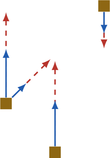
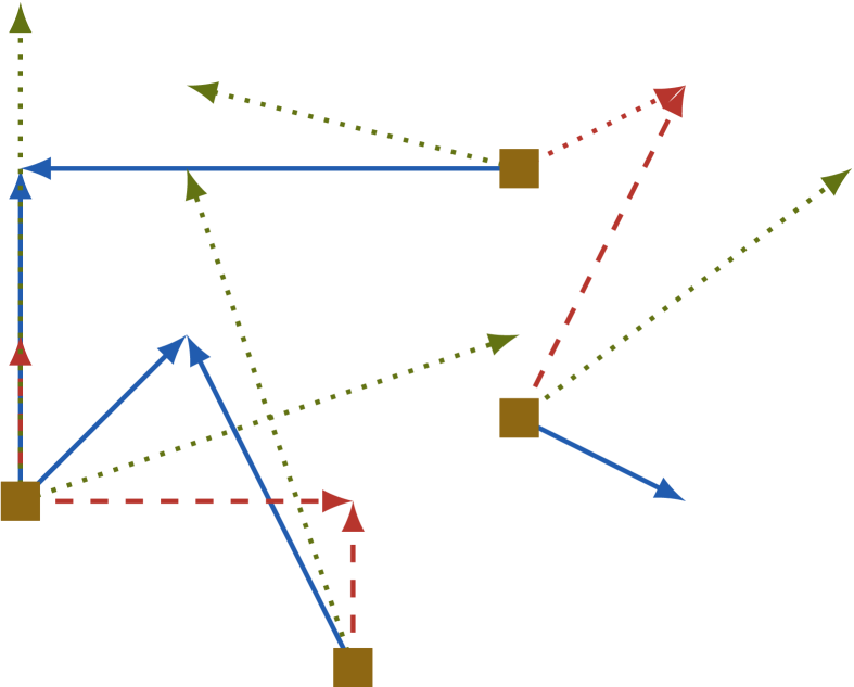
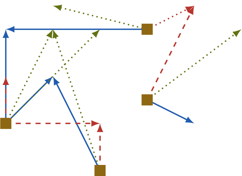
Figure 2: Wasserstein geometry. On the left, we consider example variations for ${\color[rgb]{0.55859375,0.40234375,0.07421875}\operatorname{\mu}}\in\mathcal{P}_{2}(\mathbb{R}^{d})$ (denoted by a brown square), ${\color[rgb]{0.71875,0.20703125,0.17578125}\operatorname{\xi}_{1}}$ in dotted red and ${\color[rgb]{0.12890625,0.359375,0.6875}\operatorname{\xi}_{2}}$ in solid blue. They are scaled version of each other: ${\color[rgb]{0.71875,0.20703125,0.17578125}\operatorname{\xi}_{1}}=2{\color[rgb]{0.12890625,0.359375,0.6875}\operatorname{\xi}_{2}}$. The other two images show two possible sums (in dotted green) of the variations ${\color[rgb]{0.71875,0.20703125,0.17578125}\operatorname{\xi}_{1}}$ (in dotted red) and ${\color[rgb]{0.12890625,0.359375,0.6875}\operatorname{\xi}_{2}}$ (in solid blue) at ${\color[rgb]{0.55859375,0.40234375,0.07421875}\operatorname{\mu}}\in\mathcal{P}_{2}(\mathbb{R}^{d})$: Each sum results from a different coupling $\operatorname{\alpha}\in\Gamma^{1}({\color[rgb]{0.71875,0.20703125,0.17578125}\operatorname{\xi}_{1}},{\color[rgb]{0.12890625,0.359375,0.6875}\operatorname{\xi}_{2}})$ of ${\color[rgb]{0.71875,0.20703125,0.17578125}\operatorname{\xi}_{1}}$ and ${\color[rgb]{0.12890625,0.359375,0.6875}\operatorname{\xi}_{2}}$ (i.e., different coupling of the arrows starting from the same square). The coupling resulting in the sum on the left is the one maximizing the inner product (cf. (10)) of the two variations (and, equivalently, the one attaining the minimum in the distance between the two variations; cf. (9)).

Critically, the tangent space (12) is not a vector space. However, we can equip it with an “almost” linear structure (see Figure 2 for an intuition):

Definition 2.1 (An “almost linear” structure of the tangent space).

Given $\operatorname{\bar{\mu}}\in\mathcal{P}_{2}(\mathbb{R}^{d})$, $\operatorname{\xi}_{1},\operatorname{\xi}_{2}\in\operatorname{T}_{\mathcal{P}_{2}(\mathbb{R}^{d})}(\operatorname{\bar{\mu}})$ and $\tau\in\mathbb{R}$, we define:

1. A “local” zero: $\mathbf{0}_{\operatorname{\bar{\mu}}}\coloneqq\operatorname{\bar{\mu}}\times\delta_{0}.$

2. A scalar multiplication: $\tau\operatorname{\xi}_{1}\coloneqq{(\pi_{1},\tau\pi_{2})}_{\#}{\operatorname{\xi}_{1}}.$

3. An addition: For $\operatorname{\alpha}\in\Gamma^{1}(\operatorname{\xi}_{1},\operatorname{\xi}_{2})$, $\operatorname{\xi}_{1}\,+_{\operatorname{\alpha}}\,\operatorname{\xi}_{2}\coloneqq{(\pi_{1},\pi_{2}+\pi_{3})}_{\#}{\operatorname{\alpha}}.$

In the appendix (Propositions A.6 and A.8), we show that Definition 2.1(ii)-(iii) are well-posed (i.e., $\tau\operatorname{\xi}$ and $\operatorname{\xi}_{1}\,+_{\operatorname{\alpha}}\,\operatorname{\xi}_{2}$ belong to the tangent space) as well as additional properties of this “almost linear” structure of the tangent space.

Remark 2.2.

The sum of $n$ elements $\operatorname{\xi}_{1},\ldots,\operatorname{\xi}_{n}$ results from iteratively applying Definition 2.1(iii), and we write $\operatorname{\xi}_{1}\,+_{\operatorname{\alpha}}\,\ldots\,+_{\operatorname{\alpha}}\,\operatorname{\xi}_{n}={(\pi_{1},\pi_{2}+\ldots+\pi_{n+1})}_{\#}{\operatorname{\alpha}}$ for some $\operatorname{\alpha}\in\Gamma^{1}(\operatorname{\xi}_{1},\ldots,\operatorname{\xi}_{n})$.

Comparison with the literature

Most of the literature uses the tangent space of optimal transport maps,

$$\overline{\left\{\nabla{\varphi}\,|\,\varphi\in C_{c}^{\infty}(\mathbb{R}^{d})\right\}}^{L^{2}(\mathbb{R}^{d};\operatorname{\bar{\mu}})}\\ =\overline{\left\{\varepsilon(T-\mathrm{Id})\,|\,{(\mathrm{Id},T)}_{\#}{\operatorname{\bar{\mu}}}\in\Gamma_{o}(\operatorname{\bar{\mu}},{T}_{\#}{\operatorname{\bar{\mu}}}),\exists\bar{\varepsilon}>0,\forall\varepsilon\in(-\bar{\varepsilon},\bar{\varepsilon})\right\}}^{L^{2}(\mathbb{R}^{d};\operatorname{\bar{\mu}})},$$ (13)

where $C_{c}^{\infty}(\mathbb{R}^{d})$ is the set of cylindrical and infinitely differentiable functions. This (simplified) tangent space was first introduced in [33, Chapter 8] (see e.g.  [1, 27, 36, 37] and [33, Theorem 8.5.1] for the proof of the equality in (13)) and can be embedded in (12) since for $\nabla{\varphi}$ with $\varphi\in C_{c}^{\infty}(\mathbb{R}^{d})$, the tangent vector $\operatorname{\xi}={(\mathrm{Id}_{,}\nabla{\varphi})}_{\#}{\operatorname{\bar{\mu}}}$ belongs of $\operatorname{T}_{\mathcal{P}_{2}(\mathbb{R}^{d})}(\operatorname{\bar{\mu}})$ of $\mathcal{P}_{2}(\mathbb{R}^{d})$. In fact, (i) its first marginal is $\operatorname{\bar{\mu}}$ and (ii) ${(\pi_{1},\pi_{1}+\varepsilon\pi_{2})}_{\#}{\operatorname{\xi}}={(\mathrm{Id},\mathrm{Id}+\varepsilon\nabla{\varphi})}_{\#}{\operatorname{\bar{\mu}}}$ is, for $\varepsilon$ sufficiently small, a transport plan. The latter follows from $\mathrm{Id}+\varepsilon\nabla{\varphi}$ being the gradient of a convex function and, thus, an optimal transport map [1, Proposition 2.3]. While attractive for its simplicity (it is a vector space), the tangent space (13) limits the perturbations to transport maps. For absolutely continuous measures, this comes with no loss of generality in virtue of Brenier’s theorem [50]. However, for empirical probability measures (such as the ones in data-driven applications, where one has only access to a dataset consisting of a finite number of observations), the restriction to transport maps effectively limits the possible perturbations (e.g., a Dirac’s delta can only be transported to another Dirac’s delta with a transport map). Finally, the tangent space (12), with $\varepsilon$ restricted to be positive, was first defined in [33, Chapter 12]. Instead, we drop the non-negativity of $\varepsilon$, which simplifies various technical results.

2.4 Wasserstein subgradients

We now define the regular and general subgradient, along the lines of [44, Definition 8.3] and [33, §10], for the Wasserstein space. The definition is inspired from the Euclidean setting, where $\bar{\operatorname{\upsilon}}$ is a subgradient of $f:\mathbb{R}^{d}\to\bar{\mathbb{R}}$ at $x\in\mathbb{R}^{d}$ if $f(x)-f(\bar{x})\geq\left\langle\bar{\operatorname{\upsilon}},x-\bar{x}\right\rangle+o\left(\left\|x-\bar{x}\right\|\right)$ for all $x\in\mathbb{R}^{d}$. That is, if $\bar{\operatorname{\upsilon}}$ linearly lower-bounds $f$ at $\bar{x}$. General subgradients are then defined as the limits of regular subgradients. In the probability space, we can proceed analogously. In particular, we use the (local) inner product (10) and replace the displacement “$x-\bar{x}$” with ${(\pi_{1},\pi_{2}-\pi_{1})}_{\#}{\operatorname{\gamma}}$ where $\operatorname{\gamma}\in\Gamma_{o}(\operatorname{\bar{\mu}},\operatorname{\mu})$ is an optimal transport plan between $\operatorname{\bar{\mu}}$ and $\operatorname{\mu}$ (which reduces to ${(\mathrm{Id},T-\mathrm{Id})}_{\#}{\operatorname{\bar{\mu}}}$ when $\operatorname{\gamma}$ is induced by a transport map $T$):

Definition 2.3 (Wasserstein subgradients).

Consider a functional $\operatorname{\mathcal{J}}:\mathcal{P}_{2}(\mathbb{R}^{d})\to\bar{\mathbb{R}}$ and a probability measure $\operatorname{\bar{\mu}}\in\mathcal{P}_{2}(\mathbb{R}^{d})$ with $\operatorname{\mathcal{J}}(\operatorname{\bar{\mu}})\in\mathbb{R}$. For $\operatorname{\bar{\operatorname{\xi}}}\in\operatorname{T}_{\mathcal{P}_{2}(\mathbb{R}^{d})}(\operatorname{\bar{\mu}})$, we say that

1. $\operatorname{\bar{\operatorname{\xi}}}$ is a regular subgradient of $\operatorname{\mathcal{J}}$ at $\operatorname{\bar{\mu}}$, written $\operatorname{\bar{\operatorname{\xi}}}\in\hat{\partial}\operatorname{\mathcal{J}}(\operatorname{\bar{\mu}})$, if for all $\operatorname{\mu}\in\mathcal{P}_{2}(\mathbb{R}^{d})$ and all $\operatorname{\xi}\in{(\pi_{1},\pi_{2}-\pi_{1})}_{\#}{\Gamma_{o}(\operatorname{\bar{\mu}},\operatorname{\mu})}$, it holds that $\operatorname{\mathcal{J}}(\operatorname{\mu})-\operatorname{\mathcal{J}}(\operatorname{\bar{\mu}})\geq\left\langle\operatorname{\bar{\operatorname{\xi}}},\operatorname{\xi}\right\rangle_{\operatorname{\bar{\mu}}}+o\left(W_{2}\left(\operatorname{\bar{\mu}},\operatorname{\mu}\right)\right).$ Then, $\operatorname{\mathcal{J}}$ is regularly subdifferentiable at $\operatorname{\bar{\mu}}$.

2. $\operatorname{\bar{\operatorname{\xi}}}$ is a (general) subgradient of $\operatorname{\mathcal{J}}$ at $\operatorname{\bar{\mu}}$, written $\operatorname{\bar{\operatorname{\xi}}}\in\partial\operatorname{\mathcal{J}}(\operatorname{\bar{\mu}})$ if there are sequences $\operatorname{\mu}_{n}\to\operatorname{\bar{\mu}}$ with $\operatorname{\mathcal{J}}(\mu_{n})\to\operatorname{\mathcal{J}}(\mu)$ and $\operatorname{\xi}_{n}\in\hat{\partial}\operatorname{\mathcal{J}}(\operatorname{\mu}_{n})$ with $\operatorname{\xi}_{n}\to\operatorname{\bar{\operatorname{\xi}}}$. Then, $\operatorname{\mathcal{J}}$ is subdifferentiable at $\operatorname{\bar{\mu}}$.

With this definition, we can then define regular supergradients as the elements of $-\hat{\partial}(-\operatorname{\mathcal{J}})(\operatorname{\bar{\mu}})$, and supergradients as elements of $-\partial(-\operatorname{\mathcal{J}})(\operatorname{\bar{\mu}})$). We consider the Wasserstein convergence for the general subgradient since the first marginal may differ (we consider sequences $\operatorname{\mu}_{n}\to\operatorname{\bar{\mu}}$). For this reason, the general subgradient may not be in the tangent space. The regular subgradient, instead, is in the tangent space by definition. Similarly, we can then define differentiability:

Definition 2.4 (Differentiable functional).

A functional $\operatorname{\mathcal{J}}:\mathcal{P}_{2}(\mathbb{R}^{d})\to\bar{\mathbb{R}}$ is differentiable at $\operatorname{\bar{\mu}}\in\mathcal{P}_{2}(\mathbb{R}^{d})$ if it admits both a regular subgradient and supergradient at $\operatorname{\bar{\mu}}$; i.e., $-\hat{\partial}(-\operatorname{\mathcal{J}})(\operatorname{\bar{\mu}})\cap\hat{\partial}\operatorname{\mathcal{J}}(\operatorname{\bar{\mu}})\neq\emptyset.$

Wasserstein subgradients enjoy similar properties to their Euclidean counterpart:

Proposition 2.5 (Characterization of the (sub)gradients).

Consider a functional $\operatorname{\mathcal{J}}:\mathcal{P}_{2}(\mathbb{R}^{d})\to\bar{\mathbb{R}}$ and a probability measure $\operatorname{\bar{\mu}}\in\mathcal{P}_{2}(\mathbb{R}^{d})$, where $\operatorname{\mathcal{J}}(\operatorname{\bar{\mu}})\in\mathbb{R}$. Then,

1. Either $\operatorname{\mathcal{J}}$ is differentiable at $\operatorname{\bar{\mu}}$ or at least one between $\hat{\partial}\operatorname{\mathcal{J}}(\operatorname{\bar{\mu}})$ and $\hat{\partial}(-\operatorname{\mathcal{J}})(\operatorname{\bar{\mu}})$ is empty.

2. If $G:\mathcal{P}_{2}(\mathbb{R}^{d})\to\bar{\mathbb{R}}$ is a lower bound on $\operatorname{\mathcal{J}}$, i.e., $G(\operatorname{\mu})\leq\operatorname{\mathcal{J}}(\operatorname{\mu})$ for all $\operatorname{\mu}\in\mathcal{P}_{2}(\mathbb{R}^{d})$ and $G(\operatorname{\bar{\mu}})=\operatorname{\mathcal{J}}(\operatorname{\bar{\mu}})$, then $\hat{\partial}G(\operatorname{\bar{\mu}})\subseteq\hat{\partial}\operatorname{\mathcal{J}}(\operatorname{\bar{\mu}})$.

If $\operatorname{\mathcal{J}}$ is differentiable at $\operatorname{\bar{\mu}}$, the following statements hold:

1. For all $\operatorname{\xi}_{1},\operatorname{\xi}_{2}\in-\hat{\partial}(-\operatorname{\mathcal{J}})(\operatorname{\bar{\mu}})\cap\hat{\partial}\operatorname{\mathcal{J}}(\operatorname{\bar{\mu}})$, $\operatorname{\xi}_{1}=\operatorname{\xi}_{2}$. Thus, we call this unique element the gradient of $\operatorname{\mathcal{J}}$ at $\operatorname{\bar{\mu}}$, written $\nabla{\operatorname{\mathcal{J}}}(\operatorname{\bar{\mu}})$. In particular, it satisfies $\hat{\partial}\operatorname{\mathcal{J}}(\operatorname{\bar{\mu}})=\{\nabla{\operatorname{\mathcal{J}}}(\operatorname{\bar{\mu}})\}\subseteq\partial\operatorname{\mathcal{J}}(\operatorname{\bar{\mu}})$.

2. A tangent element $\operatorname{\xi}\in\operatorname{T}_{\mathcal{P}_{2}(\mathbb{R}^{d})}(\operatorname{\bar{\mu}})$ is the gradient of $\operatorname{\mathcal{J}}$ at $\operatorname{\bar{\mu}}$ if and only if for all $\operatorname{\mu}\in\mathcal{P}_{2}(\mathbb{R}^{d})$, $\operatorname{\xi}^{\prime}\in{(\pi_{1},\pi_{2}-\pi_{1})}_{\#}{\Gamma_{o}(\operatorname{\bar{\mu}},\operatorname{\mu})}$, $\operatorname{\alpha}\in\Gamma^{1}(\operatorname{\xi},\operatorname{\xi}^{\prime})$ it holds:

   $$\operatorname{\mathcal{J}}(\operatorname{\mu})-\operatorname{\mathcal{J}}(\operatorname{\bar{\mu}})=\int_{\mathbb{R}^{d}\times\mathbb{R}^{d}}\left\langle x_{2},x_{3}-x_{1}\right\rangle\mathrm{d}\operatorname{\alpha}(x_{1},x_{2},x_{3})+o\left(W_{2}\left(\operatorname{\bar{\mu}},\operatorname{\mu}\right)\right).$$ (14)

In particular, Proposition 2.5(iii) allows us to talk about the gradient. The (general) subgradient might not be a singleton, even for a differentiable functional; see [44, §8.B] for an example in $\mathbb{R}^{d}$. Proposition 2.5(iv), instead, is the analogous of $f(y)-f(x)=\nabla{f}(x)^{\top}(y-x)+o\left(\left\|x-y\right\|\right)$: Namely, Wasserstein gradients provide a “linear approximation” from below of $\operatorname{\mathcal{J}}$, with errors that are small in terms of the Wasserstein distance.

Comparison with the literature

Our definition of regular subgradient ((i) in Definition 2.4) coincides with the definition of extended Fréchet subdifferential, introduced in [33, Definition 10.3.1] and employed, for instance, in [27]. It is a weaker notion of subdifferentiability compared to the ones in [51, 1], whereby subgradients are of the form ${(\mathrm{Id},\phi)}_{\#}{\operatorname{\mu}}{}$ for some Borel map $\phi:\mathbb{R}^{d}\to\mathbb{R}^{d}$. From an optimization perspective, these definitions are however not satisfying since, as we will discuss shortly, the Wasserstein distance itself fails to be subdifferentiable at measures that are not absolutely continuous. Inspired by classical variational analysis in Euclidean spaces [44], we therefore introduce the definition of general Wasserstein subgradients ((ii) in Definition 2.3). To the best of our knowledge, this definition is novel.

2.4.1 Why do we need such machinery?

We argue that our level of sophistication is required for at least two reasons. First, already in Euclidean spaces, variational analysis is needed to deal with non-differentiable and non-convex settings; the (general) subgradient usually appears in the necessary conditions, while the horizon subgradient (which we shall discuss in Section 2.5.1) appears in the constraint qualification (e.g., see [44, Theorem 8.15] or [46, §5.1]). We do not expect things to simplify in the more general probability space. Second, the Wasserstein distance itself fails to be regularly subdifferentiable. The existing theory of gradient flows [33, 1] bypasses this complexity resorting to absolutely continuous measures. However, this introduces a substantial practical and theoretical limitation since it excludes any data-driven setting. We characterize below the general subgradient which we show instead to be always non-empty.

The Wasserstein distance is not regularly subdifferentiable

To start, we study the regular differentiability properties of the Wasserstein distance:

Proposition 2.6 (Wasserstein subgradients and optimal plans).

Consider the functional $\operatorname{\mathcal{J}}:\mathcal{P}_{2}(\mathbb{R}^{d})\to\bar{\mathbb{R}}$, $\operatorname{\mathcal{J}}(\operatorname{\mu})\coloneqq\frac{1}{2}W_{2}\left(\operatorname{\mu},\operatorname{\hat{\mu}}\right)^{2}$. Then, for any $\operatorname{\bar{\mu}}\in\mathcal{P}_{2}(\mathbb{R}^{d})$:

1. $\operatorname{\mathcal{J}}$ is regularly superdifferentiable at $\operatorname{\bar{\mu}}$ and all ${(\pi_{1},\pi_{1}-\pi_{2})}_{\#}{\operatorname{\gamma}}$ with $\operatorname{\gamma}\in\Gamma_{o}(\operatorname{\bar{\mu}},\operatorname{\hat{\mu}})$ are supergradients of $\operatorname{\mathcal{J}}$ at $\operatorname{\bar{\mu}}$.

2. If $\Gamma_{o}(\operatorname{\bar{\mu}},\operatorname{\hat{\mu}})$ is a singleton and induced by an optimal transport map (e.g., when $\operatorname{\bar{\mu}}$ is absolutely continuous), then $\operatorname{\mathcal{J}}$ is regularly sub-differentiable, and thus differentiable, at $\operatorname{\bar{\mu}}$.

3. If $\operatorname{\xi}\in\hat{\partial}\operatorname{\mathcal{J}}(\operatorname{\bar{\mu}})$, then ${(\pi_{1},\pi_{1}-\pi_{2})}_{\#}{\operatorname{\xi}}\in\Gamma_{o}(\operatorname{\bar{\mu}},\operatorname{\hat{\mu}})$.

4. If $\Gamma_{o}(\operatorname{\bar{\mu}},\operatorname{\hat{\mu}})$ is not a singleton, then $\operatorname{\mathcal{J}}$ is not regularly subdifferentiable at $\operatorname{\mu}$.

When the set of optimal transport plans consists of a unique optimal transport map $T:\mathbb{R}^{d}\to\mathbb{R}^{d}$, then $\nabla{\operatorname{\mathcal{J}}}(\operatorname{\bar{\mu}})={(\mathrm{Id},\mathrm{Id}-T)}_{\#}{\operatorname{\bar{\mu}}}$, which is formally analogous the gradient of $x\mapsto\frac{1}{2}\left\|x-\hat{x}\right\|^{2}$ being $x-\hat{x}$ in Euclidean spaces (with “$\mathrm{Id}$ as $x$” and “$T$ as $\hat{x}$”). However, Proposition 2.6 also indicates, perhaps surprisingly, that the squared Wasserstein distance from a reference measure $\operatorname{\hat{\mu}}$ is not subdifferentiable at all measures $\operatorname{\bar{\mu}}$ for which there exist multiple optimal transport plans between $\operatorname{\bar{\mu}}$ and $\operatorname{\hat{\mu}}$. Instead, it is regularly differentiable, and thus differentiable, whenever there is a unique optimal transport plan between $\operatorname{\bar{\mu}}$ and $\operatorname{\hat{\mu}}$ and this plan is induced by an optimal transport map, a result first established in [33, Theorem 10.2.6]. By Brenier’s theorem [52], if $\operatorname{\bar{\mu}}$ is absolutely continuous, then there is a unique optimal transport plan induced by an optimal transport map between $\operatorname{\bar{\mu}}$ and $\operatorname{\hat{\mu}}$, and so the squared Wasserstein distance is differentiable at absolutely continuous measures. This result is sharp: Even when a single optimal transport plan exists, the Wasserstein distance may lack regular subgradients, as we illustrate in the next example.

Example 2.7 (Non regular-subdifferentiability of the squared Wasserstein distance).

Let $\operatorname{\bar{\mu}}\coloneqq\delta_{(0,0)}$ (blue in the picture) and $\operatorname{\hat{\mu}}\coloneqq\frac{1}{2}\delta_{(-1,0)}+\frac{1}{2}\delta_{(1,0)}$ (red in the picture). Applying the definition of Wasserstein distance (cf. (8)), $\operatorname{\mathcal{J}}({\color[rgb]{0.12890625,0.359375,0.6875}\operatorname{\bar{\mu}}})=\frac{1}{2}W_{2}\left({\color[rgb]{0.12890625,0.359375,0.6875}\operatorname{\bar{\mu}}},{\color[rgb]{0.71875,0.20703125,0.17578125}\operatorname{\hat{\mu}}}\right)^{2}=\frac{1}{2}$, and there is a unique optimal transport plan between $\operatorname{\bar{\mu}}$ and $\operatorname{\hat{\mu}}$; in particular, $\Gamma_{o}({\color[rgb]{0.12890625,0.359375,0.6875}\operatorname{\bar{\mu}}},{\color[rgb]{0.71875,0.20703125,0.17578125}\operatorname{\hat{\mu}}})=\{{\color[rgb]{0.12890625,0.359375,0.6875}\operatorname{\bar{\mu}}}\times{\color[rgb]{0.71875,0.20703125,0.17578125}\operatorname{\hat{\mu}}}\}$. We now show that $\operatorname{\mathcal{J}}(\operatorname{\mu})=\frac{1}{2}W_{2}\left(\operatorname{\mu},{\color[rgb]{0.71875,0.20703125,0.17578125}\operatorname{\hat{\mu}}}\right)^{2}$ is not regularly subdifferentiable at ${\color[rgb]{0.12890625,0.359375,0.6875}\operatorname{\bar{\mu}}}$. By Proposition 2.6(iii), it suffices to prove that $\operatorname{\xi}={(\pi_{1},\pi_{1}-\pi_{2})}_{\#}{({\color[rgb]{0.12890625,0.359375,0.6875}\operatorname{\bar{\mu}}}\times{\color[rgb]{0.71875,0.20703125,0.17578125}\operatorname{\hat{\mu}}})}=\frac{1}{2}\delta_{(0,-1)}+\frac{1}{2}\delta_{(0,1)}$ is not a regular subgradient of $\operatorname{\mathcal{J}}$.

Consider ${\color[rgb]{0.3828125,0.44921875,0.07421875}\operatorname{\mu}_{n}=\frac{1}{2}\delta_{(-\frac{1}{n},-\frac{1}{n})}+\frac{1}{2}\delta_{(\frac{1}{n},\frac{1}{n})}}$. Then, there is a unique optimal transport plan $\Gamma_{o}({\color[rgb]{0.12890625,0.359375,0.6875}\operatorname{\bar{\mu}}},{\color[rgb]{0.3828125,0.44921875,0.07421875}\operatorname{\mu}_{n}})=\{{\color[rgb]{0.12890625,0.359375,0.6875}\operatorname{\bar{\mu}}}\times{\color[rgb]{0.3828125,0.44921875,0.07421875}\operatorname{\mu}_{n}}\}$, and $\operatorname{\mathcal{J}}({\color[rgb]{0.3828125,0.44921875,0.07421875}\operatorname{\mu}_{n}})=\frac{1}{2}W_{2}\left({\color[rgb]{0.3828125,0.44921875,0.07421875}\operatorname{\mu}_{n}},{\color[rgb]{0.71875,0.20703125,0.17578125}\operatorname{\hat{\mu}}}\right)^{2}=\frac{1}{2}((1-\frac{1}{n})^{2}+\frac{1}{n^{2}})=\frac{1}{2}-\frac{1}{n}+\frac{1}{n^{2}}$, and $W_{2}\left({\color[rgb]{0.12890625,0.359375,0.6875}\operatorname{\bar{\mu}}},{\color[rgb]{0.3828125,0.44921875,0.07421875}\operatorname{\mu}_{n}}\right)=(\frac{1}{n^{2}}+\frac{1}{n^{2}})^{1/2}=\frac{\sqrt{2}}{n}$. We now show that such a sequence contradicts  Definition 2.3(i) by proving that, along this “direction”, $\operatorname{\xi}$ does not lower bound $J$. For this, we consider the variations $\operatorname{\xi}_{n}\in{(\pi_{1},\pi_{1}-\pi_{2})}_{\#}{\Gamma_{o}({\color[rgb]{0.12890625,0.359375,0.6875}\operatorname{\bar{\mu}}},{\color[rgb]{0.3828125,0.44921875,0.07421875}\operatorname{\mu}_{n}})}$. Using the expressions of ${\color[rgb]{0.12890625,0.359375,0.6875}\operatorname{\bar{\mu}}}$ and ${\color[rgb]{0.3828125,0.44921875,0.07421875}\operatorname{\mu}_{n}}$, we conclude that the only variation between $\operatorname{\bar{\mu}}$ and $\operatorname{\mu}_{n}$ is $\operatorname{\xi}_{n}={(\pi_{1},\pi_{2}-\pi_{1})}_{\#}{({\color[rgb]{0.12890625,0.359375,0.6875}\operatorname{\bar{\mu}}}\times{\color[rgb]{0.3828125,0.44921875,0.07421875}\operatorname{\mu}_{n}})}=\frac{1}{2}\delta_{(0,-\frac{1}{n})}+\frac{1}{2}\delta_{(0,\frac{1}{n})}$.

With this, we compute the inner product between $\operatorname{\xi}$ and $\operatorname{\xi}_{n}$:

$$\left\langle\operatorname{\xi},\operatorname{\xi}_{n}\right\rangle_{\operatorname{\bar{\mu}}}=\max_{\operatorname{\alpha}\in\Gamma^{1}(\operatorname{\xi},\operatorname{\xi}_{n})}\int_{\mathbb{R}^{d}\times\mathbb{R}^{d}\times\mathbb{R}^{d}}\left\langle\operatorname{\upsilon},\operatorname{\upsilon}_{n}\right\rangle\mathrm{d}\operatorname{\alpha}(x,\operatorname{\upsilon},\operatorname{\upsilon}_{n}).$$

Since $\operatorname{\alpha}$ is a coupling between $\frac{1}{2}\delta_{(0,-1)}+\frac{1}{2}\delta_{(0,1)}$ and $\frac{1}{2}\delta_{(0,-\frac{1}{n})}+\frac{1}{2}\delta_{(0,\frac{1}{n})}$, it is fully parametrized by a single coefficient $\tau\in[0,1]$, and the max reduces to a line search:

$$\left\langle\operatorname{\xi},\operatorname{\xi}_{n}\right\rangle_{\operatorname{\bar{\mu}}} =\max_{\tau\in[0,1]}\frac{\tau}{2}\left(\left\langle(1,0),\left(\frac{1}{n},\frac{1}{n}\right)\right\rangle+\left\langle(-1,0),\left(-\frac{1}{n},-\frac{1}{n}\right)\right\rangle\right)$$

$$\qquad\qquad+\frac{(1-\tau)}{2}\left(\left\langle(1,0),\left(-\frac{1}{n},-\frac{1}{n}\right)\right\rangle+\left\langle(-1,0),\left(\frac{1}{n},\frac{1}{n}\right)\right\rangle\right)=\frac{1}{n}.$$

Thus,

$$\liminf_{n\to\infty}\frac{\operatorname{\mathcal{J}}({\color[rgb]{0.3828125,0.44921875,0.07421875}\operatorname{\mu}_{n}})-\operatorname{\mathcal{J}}({\color[rgb]{0.12890625,0.359375,0.6875}\operatorname{\bar{\mu}}})-\left\langle\operatorname{\xi},\operatorname{\xi}_{n}\right\rangle_{\operatorname{\bar{\mu}}}}{W_{2}\left(\operatorname{\bar{\mu}},{\color[rgb]{0.3828125,0.44921875,0.07421875}\operatorname{\mu}_{n}}\right)}=\liminf_{n\to\infty}\frac{-\frac{2}{n}+\frac{1}{n^{2}}}{\frac{\sqrt{2}}{n}}=-\sqrt{2}<0$$

and so $\operatorname{\mathcal{J}}({\color[rgb]{0.3828125,0.44921875,0.07421875}\operatorname{\mu}_{n}})-\operatorname{\mathcal{J}}({\color[rgb]{0.12890625,0.359375,0.6875}\operatorname{\bar{\mu}}})<\left\langle\operatorname{\xi},\operatorname{\xi}_{n}\right\rangle_{\operatorname{\bar{\mu}}}+o\left(W_{2}\left({\color[rgb]{0.12890625,0.359375,0.6875}\operatorname{\bar{\mu}}},{\color[rgb]{0.3828125,0.44921875,0.07421875}\operatorname{\mu}_{n}}\right)\right)$ That is, $\operatorname{\mathcal{J}}$ is not regularly subdifferentiable at $\operatorname{\bar{\mu}}$ and, in particular, uniqueness of the optimal plan does not imply regular subdifferentiability.

The absence of regular subgradients prompts us to study the general subgradient of the Wasserstein distance. We will do so in the next section.

The (general) subgradient of the Wasserstein distance

The subdifferentiability of the Wasserstein distance at absolutely continuous probability measures (cf. Proposition 2.6(ii)) fuels the hope that the general subgradient can be characterized by approximating each probability measure via absolutely continuous ones. We illustrate the intuition by approximating a Dirac’s delta at 0 with Gaussian probability measures with vanishing variance:

Example 2.8 (Subgradients via Gaussians).

Let $\operatorname{\mathcal{J}}:\mathcal{P}_{2}(\mathbb{R}^{d})\to\bar{\mathbb{R}}$, $\operatorname{\mathcal{J}}(\operatorname{\mu})=\frac{1}{2}W_{2}\left(\operatorname{\mu},\operatorname{\hat{\mu}}\right)^{2}$ and fix $\operatorname{\bar{\mu}}=\delta_{0}$ and $\operatorname{\hat{\mu}}=\mathcal{N}\left(0,I_{d}\right)$ being the Gaussian centered in $0$ with covariance matrix $I_{d}$, the identity matrix in $\mathbb{R}^{d\times d}$. In this case, there is a unique plan $\operatorname{\bar{\mu}}\times\operatorname{\hat{\mu}}$ from $\operatorname{\bar{\mu}}$ to $\operatorname{\hat{\mu}}$, but it is not induced by a transport map (indeed, the mass at 0 needs to be split, see the picture below for an intuition). Here, we show that $\operatorname{\xi}={(\pi_{1},\pi_{1}-\pi_{2})}_{\#}{(\operatorname{\bar{\mu}}\times\operatorname{\hat{\mu}})}$ belongs to the general subgradient $\partial\operatorname{\mathcal{J}}(\operatorname{\bar{\mu}})$. To do so, we approximate $\delta_{0}$ with Gaussians with vanishing variance. Specifically, consider the sequence $\operatorname{\mu}_{n}=\mathcal{N}\left(0,\frac{1}{n^{2}}I_{d}\right)$ so that $W_{2}\left(\operatorname{\bar{\mu}},\operatorname{\mu}_{n}\right)=\frac{1}{n}\searrow 0$ and $\operatorname{\mu}_{n}\to\operatorname{\bar{\mu}}$ and $\operatorname{\mathcal{J}}(\operatorname{\mu}_{n})\to\operatorname{\mathcal{J}}(\operatorname{\bar{\mu}})$. Since both $\operatorname{\bar{\mu}}$ and $\operatorname{\mu}_{n}$ are Gaussians, the optimal transport plans is a singleton $\Gamma_{o}(\operatorname{\mu}_{n},\operatorname{\hat{\mu}})=\{{(\mathrm{Id},T_{n})}_{\#}{\operatorname{\mu}_{n}}\}$, where the optimal transport plan is induced by the optimal transport map $T_{n}(x)=nx$. By Proposition 2.6, $\operatorname{\mathcal{J}}$ is differentiable at $\operatorname{\mu}$ and, in particular, $\operatorname{\xi}_{n}\coloneqq{(\mathrm{Id},\mathrm{Id}-T_{n})}_{\#}{\operatorname{\mu}_{n}}\in\hat{\partial}\operatorname{\mathcal{J}}(\operatorname{\mu}_{n}).$ We now show that $\operatorname{\xi}_{n}\to\operatorname{\xi}$ and so $\operatorname{\xi}$ is a (general) subgradient of $\operatorname{\mathcal{J}}$. Convergence (in the Wasserstein topology) of the first marginal follows directly from ${(\pi_{1})}_{\#}{\operatorname{\xi}_{n}}=\operatorname{\mu}_{n}$, ${(\pi_{1})}_{\#}{\operatorname{\xi}}=\operatorname{\bar{\mu}}$, and $\operatorname{\mu}_{n}\to\operatorname{\bar{\mu}}$. For narrow convergence of the second marginal, consider $\phi\in C^{0}_{b}(\mathbb{R}^{d})$. Then,

$$\lim_{n\to\infty}\int_{\mathbb{R}^{d}}\phi(y)\mathrm{d}\operatorname{\xi}_{n}(x,y) =\lim_{n\to\infty}\int_{\mathbb{R}^{d}}\phi(x-T_{n}(x))\mathrm{d}\operatorname{\mu}_{n}(x)$$

$$=\lim_{n\to\infty}\int_{\mathbb{R}^{d}}\phi(x-T_{n}(x))\mathrm{d}({(T_{n}^{-1})}_{\#}{\operatorname{\hat{\mu}}})(x)$$

$$=\int_{\mathbb{R}^{d}}\lim_{n\to\infty}\phi\left(\frac{1}{n}x-x\right)\mathrm{d}\operatorname{\hat{\mu}}(x)$$

$$=\int_{\mathbb{R}^{d}}\phi(0-x)\mathrm{d}\operatorname{\hat{\mu}}(x)$$

$$=\int_{\mathbb{R}^{d}}\phi(y)\mathrm{d}\operatorname{\xi}(x,y),$$

where we used dominated convergence to exchange limit and integral and continuity of $\phi$. Thus, ${(\pi_{2})}_{\#}{\operatorname{\xi}_{n}}\rightharpoonup{(\pi_{2})}_{\#}{\operatorname{\xi}}$, and so $\operatorname{\xi}\in\partial\operatorname{\mathcal{J}}(\operatorname{\bar{\mu}})$, and the Wasserstein distance is sub-differentiable at $\operatorname{\bar{\mu}}$.

Since $\mathcal{P}_{2,\mathrm{abs}}(\mathbb{R}^{d})$ is dense in $\mathcal{P}_{2}(\mathbb{R}^{d})$ [40, Theorem 2.2.7], we can always construct a sequence $(\operatorname{\mu}_{n})_{n\in\mathbb{N}}\subseteq\mathcal{P}_{2,\mathrm{abs}}(\mathbb{R}^{d})$ with $\operatorname{\mu}_{n}\to\operatorname{\bar{\mu}}$, compute $\operatorname{\xi}_{n}\in\hat{\partial}\operatorname{\mathcal{J}}(\operatorname{\mu}_{n})$, which exists by absolute continuity of $\operatorname{\mu}_{n}$, and study the limit of $\operatorname{\xi}_{n}$. One way to construct such $\operatorname{\mu}_{n}$ is via convolution with a Gaussian kernel; see [33, Lemma 7.1.10]. Overall, this procedure yields a sufficient characterization (for the sake of necessary optimality conditions) of the (general) subgradient of the Wasserstein distance:

Proposition 2.9 (General subgradient of the squared Wasserstein distance).

For $\operatorname{\bar{\mu}},\operatorname{\hat{\mu}}\in\mathcal{P}_{2}(\mathbb{R}^{d})$, $\operatorname{\mathcal{J}}:\mathbb{R}^{d}\to\bar{\mathbb{R}}$, $\operatorname{\mathcal{J}}(\operatorname{\mu})=\frac{1}{2}W_{2}\left(\operatorname{\mu},\operatorname{\hat{\mu}}\right)^{2}$, we have $\partial\operatorname{\mathcal{J}}(\operatorname{\bar{\mu}})\neq\emptyset$ and $\partial\operatorname{\mathcal{J}}(\operatorname{\bar{\mu}})\subseteq{(\pi_{1},\pi_{1}-\pi_{2})}_{\#}{\Gamma_{o}(\operatorname{\bar{\mu}},\operatorname{\hat{\mu}})}$.

In particular, Proposition 2.9 establishes subdifferentiability of the Wasserstein distance at all probability measures $\operatorname{\bar{\mu}}\in\mathcal{P}_{2}(\mathbb{R}^{d})$.

2.4.2 Examples of subgradients

Next, we characterize the subgradients of several functionals of interest. We start with general optimal transport discrepancies, defined in (7), which arise, e.g., in uncertainty propagation in dynamical systems [53, 24] and DRO [10]:

Proposition 2.10 (Optimal transport discrepancy).

Let $\operatorname{\hat{\mu}}\in\mathcal{P}_{2}(\mathbb{R}^{d})$ and let $c:\mathbb{R}^{d}\times\mathbb{R}^{d}\to\mathbb{R}_{\geq 0}$ be twice continuously differentiable with bounded Hessian. Suppose that $c$ satisfies the twist condition (i.e., $y\mapsto\nabla_{x}{c}(x,y)$ is injective for all $x\in\mathbb{R}^{d}$). Consider the functional $\operatorname{\mathcal{J}}:\mathcal{P}_{2}(\mathbb{R}^{d})\to\bar{\mathbb{R}}$, $\operatorname{\mathcal{J}}(\operatorname{\mu})\coloneqq W_{c}\left(\operatorname{\mu},\operatorname{\hat{\mu}}\right)$ as defined in (7). Then,

1. $\operatorname{\mathcal{J}}$ is proper, non-negative, and lower semi-continuous.

2. At any $\operatorname{\bar{\mu}}\in\mathcal{P}_{2}(\mathbb{R}^{d})$, $\operatorname{\mathcal{J}}$ is subdifferentiable with $\emptyset\neq\partial\operatorname{\mathcal{J}}(\operatorname{\bar{\mu}})\subseteq{(\pi_{1},\nabla_{x}{c})}_{\#}{\Gamma_{c}(\operatorname{\bar{\mu}},\operatorname{\hat{\mu}})}$, where $\Gamma_{c}(\operatorname{\bar{\mu}},\operatorname{\hat{\mu}})$ is the set of transport plans between $\operatorname{\bar{\mu}}$ and $\operatorname{\hat{\mu}}$ that yields the minimum for $W_{c}\left(\operatorname{\mu},\operatorname{\hat{\mu}}\right)$. Moreover, if $\Gamma_{c}(\operatorname{\bar{\mu}},\operatorname{\hat{\mu}})$ is a singleton and induced by an optimal transport map (e.g., $\operatorname{\bar{\mu}}$ is absolutely continuous), then $\operatorname{\mathcal{J}}$ is differentiable with $\nabla{\operatorname{\mathcal{J}}}(\operatorname{\bar{\mu}})={(\pi_{1},\nabla_{x}{c})}_{\#}{\operatorname{\xi}},$ where $\operatorname{\xi}$ is the unique element in $\Gamma_{c}(\operatorname{\bar{\mu}},\operatorname{\hat{\mu}})$.

As already observed for the Wasserstein distance, optimal transport discrepancies are subdifferentiable (but not regularly subdifferentiable), and their subgradient is characterized in terms of the gradient of the transportation cost and the set of optimal transport plans. As a notable special case, consider $\operatorname{\bar{\mu}}=\delta_{\bar{x}}$ and $\operatorname{\hat{\mu}}=\delta_{\hat{x}}$. Then, $\operatorname{\mathcal{J}}(\operatorname{\bar{\mu}})=W_{c}\left(\operatorname{\bar{\mu}},\operatorname{\hat{\mu}}\right)=c(x,\hat{x})$ and $\Gamma_{c}(\operatorname{\bar{\mu}},\operatorname{\hat{\mu}}))=\{\delta_{(\bar{x},\hat{x})}\}$. Thus, $\operatorname{\mathcal{J}}$ is Wasserstein differentiable with gradient $\nabla{\operatorname{\mathcal{J}}}(\operatorname{\bar{\mu}})={(\pi_{1},\nabla_{x}{c})}_{\#}{\delta_{(\bar{x},\hat{x})}}=\delta_{\bar{x}}\times\delta_{\nabla_{x}{c}(\bar{x},\hat{x})}$, which is formally analogous to the standard Euclidean gradient of $x\mapsto c(x,\hat{x})$. We now exemplify our results in the case of strictly convex transportation costs:

Example 2.11 (Strictly convex transportation cost).

Consider $c(x,y)=h(x-y)$ for $h:\mathbb{R}^{d}\to\mathbb{R}_{\geq 0}$ strictly convex and twice continuously differentiable with bounded Hessian. By strict convexity of $h$, $y\mapsto\nabla_{x}{c}(x,y)=\nabla{h}(x-y)$ is injective. Thus, $c$ satisfies the assumptions of Proposition 2.10 and the subgradient of $\operatorname{\mathcal{J}}(\operatorname{\mu})\coloneqq W_{c}\left(\operatorname{\mu},\operatorname{\hat{\mu}}\right)$ at $\operatorname{\bar{\mu}}$ is $\emptyset\neq\partial\operatorname{\mathcal{J}}(\operatorname{\bar{\mu}})\subseteq{(\pi_{1},\nabla{h}\circ(\pi_{1}-\pi_{2}))}_{\#}{\Gamma_{c}(\operatorname{\bar{\mu}},\operatorname{\hat{\mu}})}$. Moreover, $\operatorname{\mathcal{J}}$ is differentiable whenever $\Gamma_{c}(\operatorname{\bar{\mu}},\operatorname{\hat{\mu}})$ is a singleton and induced by an optimal transport map and, in particular, at all absolutely continuous measures.

Next, we recall and extend, by characterizing their general subgradients, the existing subdifferentiability results for expected values:

Proposition 2.12 (Expected value).

Let $V:\mathbb{R}^{d}\to(-\infty,+\infty]$ be a proper, $\lambda$-convex, lower semicontinuous functional whose negative part has $2$-growth, i.e. $V(x)\geq-A-B\left\|x\right\|^{2}$ for all $x\in\mathbb{R}^{d}$ and for some $A,B\in\mathbb{R}$. Consider the functional $\operatorname{\mathcal{J}}:\mathcal{P}_{2}(\mathbb{R}^{d})\to\bar{\mathbb{R}}$, $\operatorname{\mathcal{J}}(\operatorname{\mu})\coloneqq\mathbb{E}^{x\sim\operatorname{\mu}}\left[V(x)\right].$ Then,

1. $\operatorname{\mathcal{J}}$ is proper and lower semi-continuous.

2. At every $\operatorname{\bar{\mu}}\in\mathcal{P}_{2}(\mathbb{R}^{d})$ at which $\operatorname{\mathcal{J}}$ is finite, $\operatorname{\xi}\in\operatorname{T}_{\mathcal{P}_{2}(\mathbb{R}^{d})}(\operatorname{\bar{\mu}})$ is in $\hat{\partial}\operatorname{\mathcal{J}}(\operatorname{\bar{\mu}})$ (resp., $\partial\operatorname{\mathcal{J}}(\operatorname{\bar{\mu}})$) if and only if for all $(x,y)\in\operatorname{supp}{(\operatorname{\xi})}$, $y\in\hat{\partial}V(x)$ (resp., $\partial V(x)$).

3. Since the Euclidean regular and general subgradients of $V$ coincides (cf. Proposition A.1), $\hat{\partial}V(x)=\partial V(x)$, we have that $\hat{\partial}\operatorname{\mathcal{J}}(\operatorname{\bar{\mu}})=\partial\operatorname{\mathcal{J}}(\operatorname{\bar{\mu}})$.

4. If $V$ is differentiable and $V(x)\leq A+B\left\|x\right\|^{2}$, $\operatorname{\mathcal{J}}$ is differentiable at any $\operatorname{\bar{\mu}}\in\mathcal{P}_{2}(\mathbb{R}^{d})$ and $\nabla{\operatorname{\mathcal{J}}}(\operatorname{\bar{\mu}})={(\mathrm{Id},\nabla{V})}_{\#}{\operatorname{\bar{\mu}}}.$

Any twice continuously differentiable function $V$ with bounded Hessian is $\lambda$-convex and satisfies $\absolutevalue{V(x)}\leq A+B\left\|x\right\|^{2}$ for some $A,B\in\mathbb{R}$. Thus, the corresponding functional $\operatorname{\mathcal{J}}$ is differentiable and, in particular, $(x,y)\in\operatorname{supp}(\nabla{\operatorname{\mathcal{J}}})$ if and only if $y=\nabla{V}(x)$. If, instead, $V$ does not have negative quadratic growth, then $\operatorname{\mathcal{J}}$ is not proper and might evaluate to $-\infty$ (e.g., $V(x)=-e^{x}$ and $\operatorname{\mu}=\mathcal{N}\left(0,1\right)$). Similarly, if $V$ grows more than quadratically, then $\operatorname{\mathcal{J}}$ will attain $+\infty$ (e.g., $V(x)=e^{x}$ and $\operatorname{\mu}=\mathcal{N}\left(0,1\right)$) and cannot be differentiable there.

Example 2.13 (Expected values of linear functions).

Consider the same functional $\operatorname{\mathcal{J}}$ as in Section 1, namely $\operatorname{\mathcal{J}}(\operatorname{\mu})=\mathbb{E}^{x\sim\operatorname{\mu}}\left[\left\langle\theta,x\right\rangle\right]$ and $V(x)=\left\langle\theta,x\right\rangle$ in Proposition 2.12. Since $V$ is a linear function, it satisfies all the assumptions of Proposition 2.12, and in particular $\operatorname{\mathcal{J}}$ is Wasserstein differentiable with $\nabla{\operatorname{\mathcal{J}}}(\operatorname{\mu})={(\mathrm{Id},\theta)}_{\#}{\operatorname{\mu}}$.

Finally, we extend the existing subdifferentiability results for interaction-type functionals which model the energy associated with the interaction between particles in a distribution; e.g., see [54] for an introduction, [55] for an example in physics, and [56, §3.3] for one in economics.

Proposition 2.14 (Interaction energy).

Let $U:\mathbb{R}^{d}\to\mathbb{R}$ be twice continuously differentiable with bounded Hessian and consider the functional $\operatorname{\mathcal{J}}:\mathcal{P}_{2}(\mathbb{R}^{d})\to\bar{\mathbb{R}}$, $\operatorname{\mathcal{J}}(\operatorname{\mu})\coloneqq\frac{1}{2}\mathbb{E}^{(x,y)\sim\operatorname{\mu}\times\operatorname{\mu}}\left[U(x-y)\right].$ Then,

1. $\operatorname{\mathcal{J}}$ is proper and continuous.

2. $\operatorname{\mathcal{J}}$ is Wasserstein differentiable and its Wasserstein gradient at $\operatorname{\bar{\mu}}\in\mathcal{P}_{2}(\mathbb{R}^{d})$ is $\nabla{\operatorname{\mathcal{J}}}(\operatorname{\bar{\mu}})={(\mathrm{Id},(\nabla{U}\ast\operatorname{\bar{\mu}}))}_{\#}{\operatorname{\bar{\mu}}},$ where $\ast$ denotes the convolution operation,

   $$(\nabla{U}\ast\operatorname{\bar{\mu}})(x)\coloneqq\int_{\mathbb{R}^{d}}U(x-y)\mathrm{d}\operatorname{\bar{\mu}}(y).$$

We exemplify the result in the case of quadratic functions:

Example 2.15 (Quadratic interaction energies).

Consider $U(z)=\frac{1}{2}\left\langle Qz,z\right\rangle$ for $Q\in\mathbb{R}^{d\times d}$. Then, $U$ is twice continuosly differentiable with $\nabla{U}(z)=Qz$ and constant (and, thus, bounded) Hessian $Q$. In virtue of Proposition 2.14, the functional $\operatorname{\mathcal{J}}(\operatorname{\mu})=\frac{1}{2}\mathbb{E}^{(x,y)\sim\operatorname{\mu}\times\operatorname{\mu}}\left[U(x-y)\right]$ is Wasserstein differentiable with $\nabla{\operatorname{\mathcal{J}}}(\operatorname{\mu})={(\mathrm{Id},Q\mathbb{E}^{x\sim\operatorname{\mu}}\left[x\right])}_{\#}{\operatorname{\mu}}.$

2.4.3 Subdifferential calculus

We now show some useful calculus rules in the Wasserstein space. More can be studied, and we expect this to be a source of interesting future work.

Proposition 2.16 (Subdifferential calculus).

Consider the proper functionals $\operatorname{\mathcal{J}}_{1},\operatorname{\mathcal{J}}_{2}:\mathcal{P}_{2}(\mathbb{R}^{d})\to\bar{\mathbb{R}}$, a monotone map $g:\bar{\mathbb{R}}\to\bar{\mathbb{R}}$ with $g(\infty)=\infty$, and $\operatorname{\bar{\mu}}\in\mathcal{P}_{2}(\mathbb{R}^{d})$ so that $\operatorname{\mathcal{J}}_{i}(\operatorname{\bar{\mu}})\in\mathbb{R}$, $g$ is continuously differentiable at $\operatorname{\mathcal{J}}_{1}(\operatorname{\bar{\mu}})\in\mathbb{R}$ with $g(\operatorname{\mathcal{J}}_{1}(\operatorname{\bar{\mu}}))\in\mathbb{R}$, and $\operatorname{\mathcal{J}}_{1}$ continuous in the Wasserstein topology at $\operatorname{\bar{\mu}}$. Then, the following rules hold:

1. Sum rule:

   $$\hat{\partial}(\operatorname{\mathcal{J}}_{1}+\operatorname{\mathcal{J}}_{2})(\operatorname{\bar{\mu}}) \supseteq\hat{\partial}(\operatorname{\mathcal{J}}_{1})(\operatorname{\bar{\mu}})+\hat{\partial}(\operatorname{\mathcal{J}}_{2})(\operatorname{\bar{\mu}})$$

   $$\coloneqq\left\{\operatorname{\xi}_{1}\,+_{\operatorname{\alpha}}\,\operatorname{\xi}_{2}\,|\,\operatorname{\xi}_{i}\in\hat{\partial}\operatorname{\mathcal{J}}_{i}(\operatorname{\bar{\mu}}),\operatorname{\alpha}\in\Gamma^{1}(\operatorname{\xi}_{1},\operatorname{\xi}_{2})\right\}.$$

   In particular, if $\operatorname{\mathcal{J}}_{2}$ is differentiable at $\operatorname{\bar{\mu}}$, then

   $$\hat{\partial}(\operatorname{\mathcal{J}}_{1}+\operatorname{\mathcal{J}}_{2})(\operatorname{\bar{\mu}}) =\hat{\partial}(\operatorname{\mathcal{J}}_{1})(\operatorname{\bar{\mu}})+\{\nabla{\operatorname{\mathcal{J}}}_{2}(\operatorname{\bar{\mu}})\}$$

   and, thus,

   $$\partial(\operatorname{\mathcal{J}}_{1}+\operatorname{\mathcal{J}}_{2})(\operatorname{\bar{\mu}}) =\partial\operatorname{\mathcal{J}}_{1}(\operatorname{\bar{\mu}})+\left\{\nabla{\operatorname{\mathcal{J}}_{2}}(\operatorname{\bar{\mu}})\right\}.$$

2. Chain rule: If $g^{\prime}(\operatorname{\mathcal{J}}_{1}(\operatorname{\bar{\mu}}))>0$, then

   $$\hat{\partial}(g\circ\operatorname{\mathcal{J}}_{1})(\operatorname{\bar{\mu}}) =g^{\prime}(\operatorname{\mathcal{J}}_{1}(\operatorname{\bar{\mu}})){\hat{\partial}\operatorname{\mathcal{J}}_{1}(\operatorname{\bar{\mu}})}$$

   $$\coloneqq\{g^{\prime}(\operatorname{\mathcal{J}}_{1}(\operatorname{\bar{\mu}}))\operatorname{\xi}\,|\,\operatorname{\xi}\in\hat{\partial}\operatorname{\mathcal{J}}_{1}(\operatorname{\bar{\mu}})\}\quad\text{and}$$

   $$\partial(g\circ\operatorname{\mathcal{J}}_{1})(\operatorname{\bar{\mu}}) =g^{\prime}(\operatorname{\mathcal{J}}_{1}(\operatorname{\bar{\mu}})){\partial\operatorname{\mathcal{J}}_{1}(\operatorname{\bar{\mu}})}.$$

With $g_{i}(x)=\rho_{i}x$ for $\rho_{1},\rho_{2}\in\mathbb{R}_{\geq 0}$, Proposition 2.16 readily characterizes the subgradients of the linear combination of functionals:

Corollary 2.17 (Linear combination rule).

Consider proper functionals $\operatorname{\mathcal{J}}_{1},\operatorname{\mathcal{J}}_{2}:\mathcal{P}_{2}(\mathbb{R}^{d})\to\bar{\mathbb{R}}$, $\rho_{1},\rho_{2}\in\mathbb{R}_{\geq 0}$, and $\operatorname{\bar{\mu}}\in\mathcal{P}_{2}(\mathbb{R}^{d})$. Then,

$$\hat{\partial}(\rho_{1}\operatorname{\mathcal{J}}_{1}+\rho_{2}\operatorname{\mathcal{J}}_{2})(\operatorname{\bar{\mu}})\supseteq\rho_{1}\hat{\partial}\operatorname{\mathcal{J}}_{1}(\operatorname{\bar{\mu}})+\rho_{2}\hat{\partial}\operatorname{\mathcal{J}}_{2}(\operatorname{\bar{\mu}}).$$

If additionally $\operatorname{\mathcal{J}}_{2}$ is differentiable,

$$\hat{\partial}(\rho_{1}\operatorname{\mathcal{J}}_{1}+\rho_{2}\operatorname{\mathcal{J}}_{2})(\operatorname{\bar{\mu}}) =\rho_{1}\hat{\partial}\operatorname{\mathcal{J}}_{1}(\operatorname{\bar{\mu}})+\rho_{2}\nabla{\operatorname{\mathcal{J}}_{2}}(\operatorname{\bar{\mu}})\quad\text{and}$$

$$\partial(\rho_{1}\operatorname{\mathcal{J}}_{1}+\rho_{2}\operatorname{\mathcal{J}}_{2})(\operatorname{\bar{\mu}}) =\rho_{1}\partial\operatorname{\mathcal{J}}_{1}(\operatorname{\bar{\mu}})+\rho_{2}\nabla{\operatorname{\mathcal{J}}_{2}}(\operatorname{\bar{\mu}}).$$

Next, we deploy Proposition 2.16 to study the variance via Proposition 2.12:

Corollary 2.18 (Variance).

Consider the functional $\operatorname{\mathcal{J}}:\mathcal{P}_{2}(\mathbb{R}^{d})\to\bar{\mathbb{R}}$, $\operatorname{\mathcal{J}}(\operatorname{\mu})\coloneqq\mathrm{Var}^{x\sim\operatorname{\mu}}\left[V(x)\right].$ If both $V$ and $x\mapsto V(x)^{2}$ satisfy the assumptions of Proposition 2.12, at every $\operatorname{\bar{\mu}}\in\mathcal{P}_{2}(\mathbb{R}^{d})$ at which $\operatorname{\mathcal{J}}(\operatorname{\bar{\mu}})\in\mathbb{R}$,

$$\partial\operatorname{\mathcal{J}}(\operatorname{\bar{\mu}}) =\hat{\partial}\operatorname{\mathcal{J}}(\operatorname{\bar{\mu}})={(\pi_{1},2(\pi_{1}-\mathbb{E}^{x\sim\operatorname{\bar{\mu}}}\left[V(x)\right])\pi_{2})}_{\#}{\biggl{\{}\operatorname{\xi}\in\operatorname{T}_{\mathcal{P}_{2}(\mathbb{R}^{d})}(\operatorname{\bar{\mu}})\,|\,\operatorname{supp}{(\operatorname{\xi})}\subseteq\hat{\partial}V\biggr{\}}}$$

When $V$ is continuously differentiable and $V(x)^{2},V(x)^{4}\leq A+B\left\|x\right\|^{2}$ for some $A,B>0$, $\operatorname{\mathcal{J}}$ is differentiable and its gradient is $\nabla{\operatorname{\mathcal{J}}}(\operatorname{\bar{\mu}})={(\mathrm{Id},2(V-\mathbb{E}^{x\sim\operatorname{\mu}}\left[V(x)\right])\nabla{V})}_{\#}{\operatorname{\bar{\mu}}}.$

2.5 Variational geometry

In this section, we study the geometry of the constraint set $\operatorname{\mathcal{C}}$, which we will combine in Section 3 with the subdifferentability of the objective function to derive our necessary optimality conditions. Similarly to Euclidean settings, all the necessary information is encoded in tangent and normal cones (see Figure 3 for an intuition in $\mathbb{R}^{d}$). We start with the tangent cone:

Definition 2.19 (Tangent cone).

The tangent cone of $\operatorname{\mathcal{C}}\subseteq\mathcal{P}_{2}(\mathbb{R}^{d})$ at $\operatorname{\bar{\mu}}\in\operatorname{\mathcal{C}}$, denoted by $\operatorname{T}_{\operatorname{\mathcal{C}}}(\operatorname{\bar{\mu}})$, is characterized by all the $\operatorname{\bar{\operatorname{\xi}}}\in\operatorname{T}_{\mathcal{P}_{2}(\mathbb{R}^{d})}(\operatorname{\bar{\mu}})$ such that for some $(\operatorname{\mu}_{n})_{n\in\mathbb{N}}\subseteq\operatorname{\mathcal{C}}$, $\operatorname{\mu}_{n}\to\operatorname{\bar{\mu}}$, $(\operatorname{\xi}_{n})_{n\in\mathbb{N}}\subseteq\operatorname{T}_{\mathcal{P}_{2}(\mathbb{R}^{d})}(\operatorname{\bar{\mu}})$, $\operatorname{\xi}_{n}\in{(\pi_{1},\pi_{2}-\pi_{1})}_{\#}{\Gamma_{o}(\operatorname{\bar{\mu}},\operatorname{\mu}_{n})}$ and $\tau_{n}\searrow 0$, one has $W_{\operatorname{\bar{\mu}}}\left(\frac{1}{\tau_{n}}\operatorname{\xi}_{n},\operatorname{\bar{\operatorname{\xi}}}\right)\to 0$.

We highlight the formal similarity with the tangent cone in Euclidean spaces, defined by all the $\bar{\operatorname{\upsilon}}$ for which there is $(x_{n})_{n\in\mathbb{N}}\subset\operatorname{\mathcal{C}}$, $x_{n}\to\bar{x}$, and $\tau_{n}\searrow 0$ so that $\frac{1}{\tau_{n}}(x_{n}-\bar{x})\to\bar{\operatorname{\upsilon}}$. In particular, if $\operatorname{\mu}_{n}=\delta_{x_{n}}$ and $\operatorname{\bar{\mu}}=\delta_{\bar{x}}$, then $\Gamma_{o}(\operatorname{\mu}_{n},\operatorname{\bar{\mu}})=\{\delta_{(x_{n},\bar{x})}\}$ and $\xi_{n}=(\bar{x},x_{n}-\bar{x})$. Namely, the definitions in the probability space and in the Euclidean space agree. Intuitively, the tangent cone is a restriction of the tangent space, and it describes the variations admissible within the set $\operatorname{\mathcal{C}}$. Dual to tangent cones are the normal cones:

Definition 2.20 (Normal cone).

The regular normal cone of $\operatorname{\mathcal{C}}\subseteq\mathcal{P}_{2}(\mathbb{R}^{d})$ at $\operatorname{\bar{\mu}}\in\operatorname{\mathcal{C}}$, denoted by $\hat{\operatorname{N}}_{\operatorname{\mathcal{C}}}(\operatorname{\bar{\mu}})$, contains all the $\operatorname{\bar{\operatorname{\xi}}}\in\operatorname{T}_{\mathcal{P}_{2}(\mathbb{R}^{d})}(\operatorname{\bar{\mu}})$ such that for all $\operatorname{\mu}\in\operatorname{\mathcal{C}}$, one has $\left\langle\operatorname{\bar{\operatorname{\xi}}},\operatorname{\xi}\right\rangle_{\operatorname{\bar{\mu}}}\leq o\left(\left\|\operatorname{\xi}\right\|_{\operatorname{\bar{\mu}}}\right)$ for $\operatorname{\xi}={(\pi_{1},\pi_{2}-\pi_{1})}_{\#}{\Gamma_{o}(\operatorname{\bar{\mu}},\operatorname{\nu})}$. The normal cone of $\operatorname{\mathcal{C}}$ at $\operatorname{\bar{\mu}}$, denoted by $\operatorname{N}_{\operatorname{\mathcal{C}}}(\operatorname{\bar{\mu}})$, is defined as the limit of regular normals; i.e., $\operatorname{\bar{\operatorname{\xi}}}\in\operatorname{T}_{\mathcal{P}_{2}(\mathbb{R}^{d})}(\operatorname{\bar{\mu}})$ belongs to $\operatorname{N}_{\operatorname{\mathcal{C}}}(\operatorname{\bar{\mu}})$ if there exists $(\operatorname{\mu}_{n})_{n\in\mathbb{N}}\subset\operatorname{\mathcal{C}}$, $\operatorname{\mu}_{n}\to\operatorname{\bar{\mu}}$, $\operatorname{\xi}_{n}\in\hat{\operatorname{N}}_{\operatorname{\mathcal{C}}}(\operatorname{\mu}_{n})$ so that $\operatorname{\xi}_{n}\to\operatorname{\bar{\operatorname{\xi}}}$.

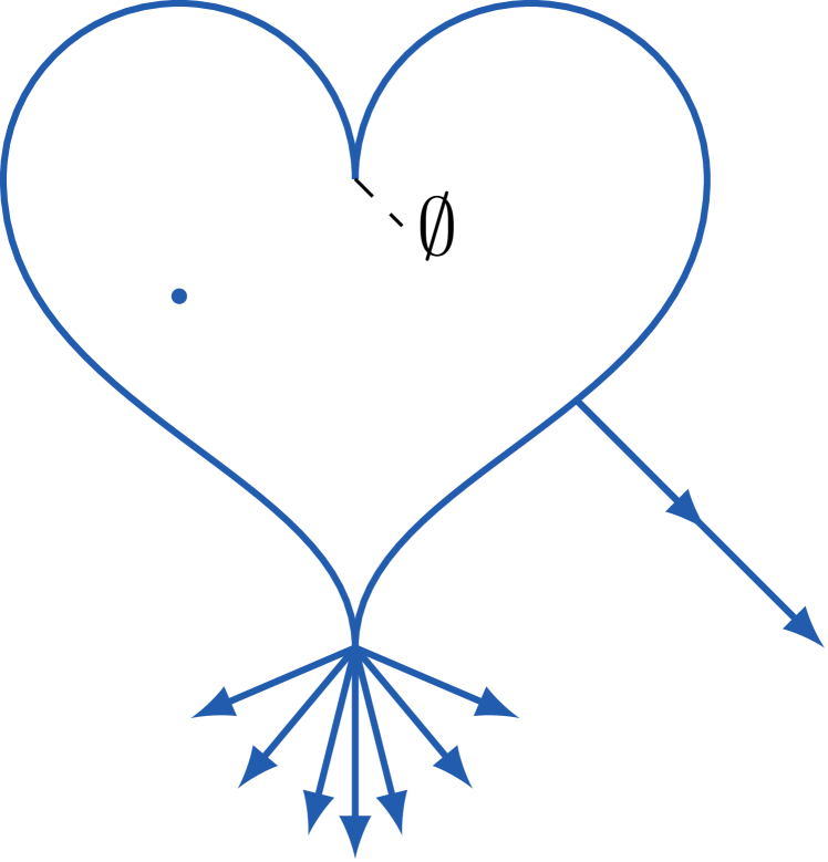
Figure 3: Variational Geometry in $\mathbb{R}^{d}$. On the left, the arrows depict some examples of regular normals (e.g., at the cusp). The interior points have a trivial normal cone, indicated by a single blue dot. At the same location $x\in\operatorname{\mathcal{C}}$ they may have different scales and directions. There also may not be any regular normal. In the middle, the solid, blue, arrows depict some examples of normals. They are the limit points of sequences of regular normals. The sequence is colored with increasing opacity as the regular normals approach the general normal. On the right, in dotted red there are sequences $\tau_{n}(x_{n}-x)\to w\in\operatorname{T}_{\mathbb{R}^{2}}(x)$, with the tangent vector $w$ being depicted in solid red. The inner product between tangent vectors and regular normals is non-positive, whereas the same might not hold with general normals.

Similarly to the subgradient definition Definition 2.3, for general normals we consider the Wasserstein convergence of regular normals. Thus, general normals may not be in the tangent space, and need not be. Analogously to the tangent cone, if we specify the definition of normal cone to Dirac’s deltas, we recover the notion of normal cone in Euclidean spaces; see also Proposition 2.22.

Another similarity to Euclidean spaces (cf. Figure 3) is the dual relationship between normal and tangent cones:

Proposition 2.21 (Normal and tangent cones relationships).

At any $\operatorname{\bar{\mu}}\in\operatorname{\mathcal{C}}\subseteq\mathcal{P}_{2}(\mathbb{R}^{d})$, the sets $\hat{\operatorname{N}}_{\operatorname{\mathcal{C}}}(\operatorname{\bar{\mu}})$ and $\operatorname{N}_{\operatorname{\mathcal{C}}}(\operatorname{\bar{\mu}})$ are closed cones. Additionally, if $\operatorname{\bar{\operatorname{\xi}}}\in\hat{\operatorname{N}}_{\operatorname{\mathcal{C}}}(\operatorname{\bar{\mu}})$ then $\left\langle\operatorname{\bar{\operatorname{\xi}}},\operatorname{\xi}\right\rangle_{\operatorname{\bar{\mu}}}\leq 0$ for all $\operatorname{\xi}\in\operatorname{T}_{\operatorname{\mathcal{C}}}(\operatorname{\bar{\mu}}).$

As a first example, we study the normal cones of trivial constraint sets:

Proposition 2.22 (Trivial normal cones).

Let $\operatorname{\mathcal{C}}\subseteq\mathcal{P}_{2}(\mathbb{R}^{d})$ and $\operatorname{\bar{\mu}}\in\operatorname{\mathcal{C}}$. Then,

1. if $\operatorname{\mathcal{C}}=\mathcal{P}_{2}(\mathbb{R}^{d})$, then $\hat{\operatorname{N}}_{\operatorname{\mathcal{C}}}(\operatorname{\bar{\mu}})=\operatorname{N}_{\operatorname{\mathcal{C}}}(\operatorname{\bar{\mu}})=\operatorname{N}_{\mathcal{P}_{2}(\mathbb{R}^{d})}(\operatorname{\bar{\mu}})=\{\mathbf{0}_{\operatorname{\bar{\mu}}}\}$;

2. if $\operatorname{\bar{\mu}}\in\mathrm{int}_{W_{2}}{\operatorname{\mathcal{C}}}$, then $\hat{\operatorname{N}}_{\operatorname{\mathcal{C}}}(\operatorname{\bar{\mu}})=\operatorname{N}_{\operatorname{\mathcal{C}}}(\operatorname{\bar{\mu}})=\{\mathbf{0}_{\operatorname{\bar{\mu}}}\}$;

3. for $\Xi\subseteq\mathbb{R}^{d}$, if $\operatorname{\mathcal{C}}\subseteq\{\delta_{x}\in\mathcal{P}_{2}(\mathbb{R}^{d})\,|\,x\in\Xi\}$, then at any $\operatorname{\bar{\mu}}=\delta_{\bar{x}}\in\operatorname{\mathcal{C}}$

   $$\hat{\operatorname{N}}_{\operatorname{\mathcal{C}}}(\operatorname{\bar{\mu}}) =\{\delta_{\bar{x}}\times\nu\,|\,\mathbb{E}^{x\sim\nu}\left[x\right]\in\hat{\operatorname{N}}_{\Xi}(\bar{x})\}\quad\text{and}$$

   $$\operatorname{N}_{\operatorname{\mathcal{C}}}(\operatorname{\bar{\mu}}) =\{\delta_{\bar{x}}\times\nu\,|\,\mathbb{E}^{x\sim\nu}\left[x\right]\in\operatorname{N}_{\Xi}(\bar{x})\},$$

   where $\hat{\operatorname{N}}_{\Xi}(\bar{x})\}$ and $\operatorname{N}_{\Xi}(\bar{x})\}$ are the regular and general normal cones in the Euclidean space, respectively.

In particular, analogously to the Euclidean setting, the normal cone at $\operatorname{\bar{\mu}}$ trivializes if the feasible set covers the whole space (Proposition 2.22(i)) or if $\operatorname{\bar{\mu}}$ lies in its interior (Proposition 2.22(ii)); cf. Figure 3. Moreover, when we restrict ourselves to the space of Dirac’s deltas, the normal cone is consistent with its Euclidean counterpart (Proposition 2.22(iii)); namely, a “tangent vector” $\nu$ lies in the normal cone if and only if its “average” tangent vector lies in the Euclidean normal cone.

Next, we characterize the normal cone of sublevel sets of functionals:

Proposition 2.23 (Level sets).

Suppose $\operatorname{\mathcal{C}}\coloneqq\left\{\operatorname{\mu}\in\mathcal{P}_{2}(\mathbb{R}^{d})\,|\,\operatorname{\mathcal{J}}(\operatorname{\mu})\leq 0\right\}$ for a proper, continuous functional $\operatorname{\mathcal{J}}:\mathcal{P}_{2}(\mathbb{R}^{d})\to\bar{\mathbb{R}}$. Then, at any $\operatorname{\bar{\mu}}\in\operatorname{\mathcal{C}}$ so that $\operatorname{\mathcal{J}}(\operatorname{\bar{\mu}})=0$, we have

$$\hat{\operatorname{N}}_{\operatorname{\mathcal{C}}}(\operatorname{\bar{\mu}})\supseteq\left\{\lambda\operatorname{\xi}\,|\,\lambda\geq 0,\operatorname{\xi}\in\hat{\partial}\operatorname{\mathcal{J}}(\operatorname{\bar{\mu}})\right\}$$ (15)

and, if $\mathbf{0}_{\operatorname{\bar{\mu}}}\not\in\partial\operatorname{\mathcal{J}}(\operatorname{\bar{\mu}})$ and $\partial\operatorname{\mathcal{J}}(\operatorname{\bar{\mu}})\neq\emptyset$, then

$$\operatorname{N}_{\operatorname{\mathcal{C}}}(\operatorname{\bar{\mu}})\subseteq\left\{\lambda\operatorname{\xi}\,|\,\lambda\geq 0,\operatorname{\xi}\in\partial\operatorname{\mathcal{J}}(\operatorname{\bar{\mu}})\right\}\cup\partial^{\infty}\operatorname{\mathcal{J}}(\operatorname{\bar{\mu}}).$$ (16)

If $\operatorname{\mathcal{J}}(\operatorname{\bar{\mu}})<0$, then $\hat{\operatorname{N}}_{\operatorname{\mathcal{C}}}(\operatorname{\bar{\mu}})=\operatorname{N}_{\operatorname{\mathcal{C}}}(\operatorname{\bar{\mu}})=\{\mathbf{0}_{\operatorname{\bar{\mu}}}\}$.

Proposition 2.23 intimately relates to Lagrange multipliers in the Wasserstein space: The normal cone of a sublevel set of a functional $\operatorname{\mathcal{J}}{}$ consists of any scaling (by a multiplier) of the subgradients of $\operatorname{\mathcal{J}}{}$. In particular, it includes the case where the constraint is not active (i.e., the multiplier is zero and the normal cone trivializes) and the case where the constraint is active (i.e., the multiplier is non-zero). The condition $\mathbf{0}_{\operatorname{\bar{\mu}}}\not\in\partial\operatorname{\mathcal{J}}(\operatorname{\bar{\mu}})$ resembles the same “constraint qualification” required in Euclidean settings (cf. [44, Proposition 10.3]), and in practice it is often not restrictive. As an example, we consider the normal cone of (closed) Wasserstein balls:

Example 2.24 (Normal cone of closed Wasserstein balls).

For some $\varepsilon>0$, consider $\operatorname{\mathcal{C}}=\bar{\mathbb{B}}_{W_{2}}(\varepsilon;\operatorname{\hat{\mu}})=\{\mu\in\mathcal{P}_{2}(\mathbb{R}^{d})\,|\,W_{2}\left(\operatorname{\mu},\operatorname{\hat{\mu}}\right)^{2}\leq\varepsilon^{2}\}$. Since at any interior point the normal cone of $\operatorname{\mathcal{C}}$ trivializes, we only need to consider $\operatorname{\bar{\mu}}$ on the boundary. By Proposition 2.9, the subgradient of the Wasserstein distance is not empty and is contained in ${(\pi_{1},2\pi_{1}-2\pi_{2})}_{\#}{\Gamma_{o}(\operatorname{\bar{\mu}},\operatorname{\hat{\mu}})}$. Since $\operatorname{\bar{\mu}}$ lies at the boundary, we have $\operatorname{\bar{\mu}}\neq\operatorname{\hat{\mu}}$ and so $\Gamma_{o}(\operatorname{\bar{\mu}},\operatorname{\hat{\mu}})$ does not contain the “identity plan” ${(\mathrm{Id},\mathrm{Id})}_{\#}{\operatorname{\bar{\mu}}}$. Thus, $\mathbf{0}_{\operatorname{\bar{\mu}}}$ does not belong to the subgradient of the Wasserstein distance, and the constraint qualification in Proposition 2.22 holds true. With this, we conclude that the normal cone satisfies

$$\operatorname{N}_{\operatorname{\mathcal{C}}}(\operatorname{\bar{\mu}})\subseteq\{\operatorname{\xi}\,|\,\operatorname{\xi}\in{(\pi_{1},2\lambda(\pi_{1}-\pi_{2}))}_{\#}{\Gamma_{o}(\operatorname{\bar{\mu}},\operatorname{\hat{\mu}})},\lambda\geq 0\}.$$

In particular, if $\operatorname{\bar{\mu}}$ is absolutely continuous, then $\Gamma_{o}(\operatorname{\bar{\mu}},\operatorname{\hat{\mu}})=\{{(\mathrm{Id},T)}_{\#}{\operatorname{\bar{\mu}}}\}$, where $T$ is the unique optimal transport map $T$, and $\operatorname{N}_{\operatorname{\mathcal{C}}}(\operatorname{\bar{\mu}})\subseteq\{{(\mathrm{Id},2\lambda(\mathrm{Id}-T))}_{\#}{\operatorname{\bar{\mu}}}\,|\,\lambda\geq 0\}.$

We also study the feasible set of the optimization problem (2), presented in Section 1, namely the second moment constraint:

Example 2.25 (Second moment constraint).

For $\varepsilon>0$, consider $\operatorname{\mathcal{C}}=\{\operatorname{\mu}\in\mathcal{P}_{2}(\mathbb{R}^{d})\,|\,\mathbb{E}^{x\sim\operatorname{\mu}}\left[\left\|x\right\|^{2}\right]\leq\varepsilon^{2}\}$. Then, $\operatorname{\mathcal{C}}=\bar{\mathbb{B}}_{W_{2}}(\varepsilon;\delta_{0})$ and, thus, for any $\operatorname{\bar{\mu}}\in\mathcal{P}_{2}(\mathbb{R}^{d})$ in the interior of $\operatorname{\mathcal{C}}$ the normal cone trivializes, whereas for all the ones with $\mathbb{E}^{x\sim\operatorname{\bar{\mu}}}\left[\left\|x\right\|^{2}\right]=\varepsilon^{2}$ we have $\operatorname{N}_{\operatorname{\mathcal{C}}}(\operatorname{\bar{\mu}})\subseteq\left\{{(\mathrm{Id},2\lambda\mathrm{Id})}_{\#}{\operatorname{\bar{\mu}}}\,|\,\lambda\geq 0\right\}.$

To prove our first-order optimality conditions in Theorem 3.2, we will require a technical property for the constraint set:

Definition 2.26 (Sequential normal compactness).

A set $\operatorname{\mathcal{C}}$ is sequentially normally compact (SNC) at $\operatorname{\bar{\mu}}$ if for any sequence $\operatorname{\mu}_{n}\to\operatorname{\bar{\mu}}$ and $\operatorname{\xi}_{n}\in\hat{\operatorname{N}}_{\operatorname{\mathcal{C}}}(\operatorname{\mu}_{n})$ so that $\operatorname{\xi}_{n}\rightharpoonup\operatorname{\xi}$, we have $\operatorname{\xi}\to\operatorname{\xi}$.

In particular, the normal cones of the sets in Examples 2.24 and 2.25 are SNC:

Proposition 2.27 (The Wasserstein ball is SNC).

The closed Wasserstein ball around $\operatorname{\hat{\mu}}$ of radius $\varepsilon>0$, $\bar{\mathbb{B}}_{W_{2}}(\varepsilon;\operatorname{\hat{\mu}})$, is SNC at all $\operatorname{\bar{\mu}}\in\bar{\mathbb{B}}_{W_{2}}(\varepsilon;\operatorname{\hat{\mu}})$.

2.5.1 Variational geometry and epigraphs

In Section 3, we provide the first-order optimality conditions for general, constrained, optimization problems and present differentiable functionals as a special case. From a technical standpoint, however, we first establish optimality conditions for differentiable functions, and then study the non-differentiable case via an epigraphical argument. This will result in a “constraint qualification” which is typical in Euclidean spaces and we find in the Wasserstein space as well. More formally, recall that the epigraph of a proper functional $\operatorname{\mathcal{J}}:\mathcal{P}_{2}(\mathbb{R}^{d})\to\bar{\mathbb{R}}$ is the set

$$\widetilde{\mathrm{epi}}\operatorname{\mathcal{J}}\coloneqq\left\{(\operatorname{\mu},\beta)\,|\,\operatorname{\mu}\in\mathcal{P}_{2}(\mathbb{R}^{d}),\operatorname{\mathcal{J}}(\operatorname{\mu})\leq\beta\right\}\subset\mathcal{P}_{2}(\mathbb{R}^{d})\times\mathbb{R}.$$

Then, we immediately observe that

$$\inf_{\operatorname{\mu}\in\operatorname{\mathcal{C}}}\operatorname{\mathcal{J}}(\operatorname{\mu})=\inf_{(\operatorname{\mu},\beta)\in\widetilde{\mathrm{epi}}(\operatorname{\mathcal{J}})\cap(\operatorname{\mathcal{C}}\times\mathbb{R})}\beta=\inf_{(\operatorname{\mu},\beta)\in\widetilde{\mathrm{epi}}(\operatorname{\mathcal{J}})\cap(\operatorname{\mathcal{C}}\times\mathbb{R})}\tilde{l}(\operatorname{\mu},\beta),$$

with $\tilde{l}:\mathcal{P}_{2}(\mathbb{R}^{d})\times\mathbb{R}\to\mathbb{R}$ being the linear function $\tilde{l}(\operatorname{\mu},\beta)=\beta$. Being linear, $\tilde{l}$ is supposedly easy to optimize. Unfortunately, this argument does not directly carry over to the Wasserstein space: While on $\mathbb{R}^{d}$ the epigraph is a subset of $\mathbb{R}^{d+1}$, on $\mathcal{P}_{2}(\mathbb{R}^{d})$ is a subset of $\mathcal{P}_{2}(\mathbb{R}^{d})\times\mathbb{R}$ and not $\mathcal{P}_{2}(\mathbb{R}^{d+1})$. Thus, one has to study the differential structure and variational geometry of $\mathcal{P}_{2}(\mathbb{R}^{d})\times\mathbb{R}$. To avoid this burden, we take a different angle. Since each $x\in\mathbb{R}^{d}$ can be “embedded” in the probability space as the Dirac’s delta $\delta_{x}\in\mathcal{P}_{2}(\mathbb{R}^{d})$, we define the epigraph as

$$\operatorname{epi}\operatorname{\mathcal{J}}\coloneqq\left\{\operatorname{\mu}\times\delta_{\beta}\,|\,\operatorname{\mu}\in\mathcal{P}_{2}(\mathbb{R}^{d}),\operatorname{\mathcal{J}}(\operatorname{\mu})\leq\beta\right\}\subseteq\mathcal{P}_{2}(\mathbb{R}^{d+1}).$$ (17)

In particular, contrary to $\widetilde{\mathrm{epi}}\operatorname{\mathcal{J}}$, $\operatorname{epi}\operatorname{\mathcal{J}}$ is now a subset of $\mathcal{P}_{2}(\mathbb{R}^{d+1})$. Then, the optimization of $\operatorname{\mathcal{J}}$ over $\operatorname{\mathcal{C}}$ is equivalent to the optimization of $l:\mathcal{P}_{2}(\mathbb{R}^{d+1})\to\mathbb{R}$, $l(\bm{\operatorname{\mu}})=\mathbb{E}^{\bm{x}\sim\bm{\operatorname{\mu}}}\left[\left\langle(0,\ldots,0,1),\bm{x}\right\rangle\right]$, over $\operatorname{epi}\operatorname{\mathcal{J}}\cap\operatorname{\mathcal{C}}_{e}$, with $\operatorname{\mathcal{C}}_{e}\coloneqq\{\operatorname{\mu}\times\delta_{\beta}\,|\,\operatorname{\mu}\in\operatorname{\mathcal{C}},\beta\in\mathbb{R}\}.$ Note that we use bold symbols when working in $\mathbb{R}^{d+1}$ and $\mathcal{P}_{2}(\mathbb{R}^{d+1})$ (e.g., $\bm{x}=(x,\beta)$ with $x\in\mathbb{R}^{d}$ and $\beta\in\mathbb{R}$). Given $\bm{\mu}$, we can “extract” $\operatorname{\mu}$ and $\delta_{\beta}$ via ${(\pi_{1},\ldots,\pi_{d})}_{\#}{\bm{\operatorname{\mu}}}=\operatorname{\mu}$ (i.e., we forget the last component) and ${(\pi_{d+1})}_{\#}{\bm{\operatorname{\mu}}}=\delta_{\beta}$ (i.e., we keep only the last component). Similarly, given a variation $\bm{\operatorname{\xi}}\in\operatorname{T}_{\mathcal{P}_{2}(\mathbb{R}^{d+1})}(\operatorname{\mu})$, we can extract the variation corresponding to $\operatorname{\mu}$ via ${T}_{\#}{\bm{\operatorname{\xi}}}$, where

$$T\coloneqq(\pi_{1},\ldots,\pi_{d},\pi_{d+2},\ldots,\pi_{2d+1})$$ (18)

(i.e., we forget the last component of the first and the second marginal), and the variation “corresponding” to $\delta_{\beta}$ via ${(\pi_{d+1},\pi_{d+2})}_{\#}{\bm{\operatorname{\xi}}}$ (i.e., we only keep the last component of the first and the second marginal). With this formalism, the gradient of $l$ follows directly from Proposition 2.12 and it reads $\bm{\operatorname{\mu}}\times\bm{\delta_{(0,\ldots,0,1)}}$. Thus, the complexity of our main result moves to prove first-order optimality conditions in the differentiable case subject to epigraphical constraints, for which, in particular, we need to study the variational geometry of $\operatorname{epi}\operatorname{\mathcal{J}}$, which we do next. To start, observe that epigraphical normals “point downwards in expectation”:

Proposition 2.28 (Characterization of the epigraphical normals).

For $\operatorname{\mathcal{J}}:\mathcal{P}_{2}(\mathbb{R}^{d})\to\bar{\mathbb{R}}$, consider $\operatorname{\bar{\mu}}\in\mathcal{P}_{2}(\mathbb{R}^{d})$ at which $\operatorname{\mathcal{J}}$ is finite. For all $\bm{\operatorname{\xi}}\in\operatorname{N}_{\operatorname{epi}\operatorname{\mathcal{J}}}(\operatorname{\bar{\mu}}\times\delta_{\operatorname{\mathcal{J}}(\operatorname{\bar{\mu}})})$ (i.e., at the boundary of $\operatorname{epi}\operatorname{\mathcal{J}}$) we have $\mathbb{E}^{(\bm{x},\bm{\operatorname{\upsilon}})\sim\bm{\operatorname{\xi}}}\left[\left\langle(0,\ldots,0,1),\bm{\operatorname{\upsilon}}\right\rangle\right]\leq 0$.

Proposition 2.28 is reminiscent of the well-known fact that, in Euclidean settings, epigraphical normals never point upwards. We depict this idea below on the right.

For the (discontinuous) function $f$ with graph depicted in black, the epigraph is the region in light green above the graph. The regular subgradients at the discontinuity point (black-filled point) correspond to the thick blue arrows, which touch the plane at $y=-1$. These arrows are also related to the normals of the epigraph, which contains their $\lambda$-scaled version as well. These are depicted in dashed blue, and they intersect the $-\lambda$ plane.

We rigorously show that the relationship between the non-horizontal normals (in expectation) to $\operatorname{epi}\operatorname{\mathcal{J}}$ and the subgradients of $\operatorname{\mathcal{J}}$ translates to the probability space:

Proposition 2.29 (Subgradients and epigraphical normals).

Let $\operatorname{\mathcal{J}}:\mathcal{P}_{2}(\mathbb{R}^{d})\to\bar{\mathbb{R}}$ and any $\operatorname{\bar{\mu}}\in\mathcal{P}_{2}(\mathbb{R}^{d})$ at which $\operatorname{\mathcal{J}}(\operatorname{\bar{\mu}})\in\mathbb{R}$ and let $\bm{\operatorname{\xi}}\in\operatorname{N}_{\operatorname{epi}\operatorname{\mathcal{J}}}(\operatorname{\bar{\mu}}\times\delta_{\operatorname{\mathcal{J}}(\operatorname{\bar{\mu}})})$ with $\mathbb{E}^{(\bm{x},\bm{\operatorname{\upsilon}})\sim\bm{\operatorname{\xi}}}\left[\left\langle(0,\ldots,0,1),\bm{v}\right\rangle\right]=-1$. Then, ${T}_{\#}{\bm{\operatorname{\xi}}}\in\partial\operatorname{\mathcal{J}}(\operatorname{\bar{\mu}})$ with $T$ as in (18).

Note that Proposition 2.29 characterizes all non-horizontal normals. Indeed, if $\bm{\operatorname{\xi}}\in\operatorname{N}_{\operatorname{epi}\operatorname{\mathcal{J}}}(\operatorname{\bar{\mu}}\times\delta_{\operatorname{\mathcal{J}}(\operatorname{\bar{\mu}})})$ satisfies $\mathbb{E}^{(\bm{x},\bm{\operatorname{\upsilon}})\sim\bm{\operatorname{\xi}}}\left[\left\langle(0,\ldots,0,1),\bm{v}\right\rangle\right]=-\lambda<0$, then, since the normal cone is a cone (cf. Proposition 2.21), $\frac{1}{\lambda}\bm{\operatorname{\xi}}$ also belongs to $\operatorname{N}_{\operatorname{epi}\operatorname{\mathcal{J}}}(\operatorname{\bar{\mu}}\times\delta_{\operatorname{\mathcal{J}}(\operatorname{\bar{\mu}})})$ and it satifies $\mathbb{E}^{(\bm{x},\bm{\operatorname{\upsilon}})\sim\frac{1}{\lambda}\bm{\operatorname{\xi}}}\left[\left\langle(0,\ldots,0,1),\bm{v}\right\rangle\right]=\mathbb{E}^{(\bm{x},\bm{\operatorname{\upsilon}})\sim\bm{\operatorname{\xi}}}\left[\left\langle(0,\ldots,0,1),\frac{1}{\lambda}\bm{v}\right\rangle\right]=-1$. Thus, ${(\pi_{1},\ldots,\pi_{d})}_{\#}{\frac{1}{\lambda}\bm{\operatorname{\xi}}}\in\partial\operatorname{\mathcal{J}}(\operatorname{\bar{\mu}})$. In Euclidean spaces, these normals are referred to as horizon subgradients (we depict one in red in the figure above). Thus, we introduce the natural counterpart in the probability space:

Definition 2.30 (Wasserstein horizon subgradients).

For $\operatorname{\mathcal{J}}:\mathcal{P}_{2}(\mathbb{R}^{d})\to\bar{\mathbb{R}}$ and any $\operatorname{\bar{\mu}}\in\mathcal{P}_{2}(\mathbb{R}^{d})$ at which $\operatorname{\mathcal{J}}(\operatorname{\bar{\mu}})\in\mathbb{R}$, we say that $\operatorname{\xi}$ is a horizon subgradient of $\operatorname{\mathcal{J}}$ at $\operatorname{\bar{\mu}}$, $\operatorname{\xi}\in\partial^{\infty}\operatorname{\mathcal{J}}(\operatorname{\bar{\mu}})$, if there exists $\bm{\operatorname{\xi}}\in\operatorname{N}_{\operatorname{epi}\operatorname{\mathcal{J}}}(\operatorname{\bar{\mu}}\times\delta_{\operatorname{\mathcal{J}}(\operatorname{\bar{\mu}})})$ such that ${T}_{\#}{\bm{\operatorname{\xi}}}=\operatorname{\xi}$ and $\mathbb{E}^{(\bm{x},\bm{\operatorname{\upsilon}})}\left[\left\langle(0,\ldots,0,1),\bm{\operatorname{\upsilon}}\right\rangle\right]=0$, with $T$ as in (18).

The horizon subgradients relate to the constraint qualifications and, as we shall see in Section 3, are required for a comprehensive theory of optimization. Similar ideas are necessary already in Euclidean spaces and, perhaps surprisingly, they naturally carry over to the probability space. Since they are defined starting from the general normals to the epigraph, they are not guaranteed to be in the tangent space. Nonetheless, for sufficiently well-behaved functionals they are trivial:

Proposition 2.31 (Horizon subgradients for strictly continuous functions).

Let $\operatorname{\mathcal{J}}:\mathcal{P}_{2}(\mathbb{R}^{d})\to\bar{\mathbb{R}}$ and any $\operatorname{\bar{\mu}}\in\mathcal{P}_{2}(\mathbb{R}^{d})$. If $\operatorname{\mathcal{J}}$ is strictly continuous at $\operatorname{\bar{\mu}}$, i.e.,

$$\limsup_{\operatorname{\mu}\to\operatorname{\bar{\mu}}}\frac{\left\|\operatorname{\mathcal{J}}(\operatorname{\mu})-\operatorname{\mathcal{J}}(\operatorname{\bar{\mu}})\right\|}{W_{2}\left(\operatorname{\mu},\operatorname{\bar{\mu}}\right)}<\infty,$$

then the horizon subgradient of $\operatorname{\mathcal{J}}$ at $\operatorname{\bar{\mu}}$ is trivial; i.e., $\partial^{\infty}\operatorname{\mathcal{J}}{\operatorname{\bar{\mu}}}=\{\mathbf{0}_{\operatorname{\bar{\mu}}}\}$.

For instance, all locally Lipschitz functionals are strictly continuous and therefore have trivial horizon subgradients. This is also the case for many of the functionals discussed so far:

Proposition 2.32 (Some horizon subgradients).

At any $\operatorname{\bar{\mu}}\in\mathcal{P}_{2}(\mathbb{R}^{d})$, the functionals defined in Propositions 2.12, 2.14, 2.10, 2.9 and 2.18 have trivial horizon subgradient $\partial^{\infty}\operatorname{\mathcal{J}}=\{\mathbf{0}_{\operatorname{\bar{\mu}}}\}$.

With horizon subgradients, we can finally provide a full characterization of epigraphical normals:

Proposition 2.33 (Subgradients and epigraphical normals).

Let $\operatorname{\mathcal{J}}:\mathcal{P}_{2}(\mathbb{R}^{d})\to\bar{\mathbb{R}}$ and $\operatorname{\bar{\mu}}\in\mathcal{P}_{2}(\mathbb{R}^{d})$ at which $\operatorname{\mathcal{J}}(\operatorname{\bar{\mu}})\in\mathbb{R}$. With $T$ as in (18), we have that $\bm{\operatorname{\xi}}\in\operatorname{N}_{\operatorname{epi}\operatorname{\mathcal{J}}}(\operatorname{\mu}\times\delta_{\operatorname{\mathcal{J}}(\operatorname{\mu})})$ if and only if either

1. $\mathbb{E}^{(\bm{x},\bm{\operatorname{\upsilon}})\sim\bm{\operatorname{\xi}}}\left[\left\langle(0,\ldots,0,1),\bm{\operatorname{\upsilon}}\right\rangle\right]=-\lambda,\lambda>0$ and $\frac{1}{\lambda}{T}_{\#}{\bm{\operatorname{\xi}}}\in\partial\operatorname{\mathcal{J}}(\operatorname{\mu})$; or

2. $\mathbb{E}^{(\bm{x},\bm{\operatorname{\upsilon}})\sim\bm{\operatorname{\xi}}}\left[\left\langle(0,\ldots,0,1),\bm{\operatorname{\upsilon}}\right\rangle\right]=0$ and ${T}_{\#}{\bm{\operatorname{\xi}}}\in\partial^{\infty}\operatorname{\mathcal{J}}(\operatorname{\mu})$.

Discussion

The definition of horizon subgradients introduced in Definition 2.30 follows the geometrical ideas used for Euclidean spaces in [47, Definition 1.18]. It departs from the alternative definition of the horizon subgradients as the scaled limit of regular subgradients [44, Definition 8.3], according to which $\operatorname{\xi}\in\partial^{\infty}\operatorname{\mathcal{J}}(\operatorname{\bar{\mu}})$ if there are sequences $\operatorname{\mu}_{n}\to\operatorname{\bar{\mu}},\operatorname{\mathcal{J}}(\operatorname{\mu}_{n})\to\operatorname{\mathcal{J}}(\operatorname{\bar{\mu}})$ and $\operatorname{\xi}_{n}\in\hat{\partial}\operatorname{\mathcal{J}}(\operatorname{\mu}_{n})$ so that there exists $(\tau_{n})_{n\in\mathbb{N}}\subseteq\mathbb{R}_{\geq 0},\tau_{n}\searrow 0$ and $\tau_{n}\operatorname{\xi}_{n}\to\operatorname{\bar{\operatorname{\xi}}}$. Nonetheless, it is well known that, at least in Euclidean settings, the two definitions are identical, cf. [44, Theorem 8.9]. Finally, we could have defined the subgradients also as the non-horizontal epigraphical normals, as in [47, Definition 1.18]. Nonetheless, to ease the presentation, we opted for the more standard Definition 2.3, as in [44, Definition 8.3].

3 Optimality conditions

In this section, we prove our main result. To start, we need a notion of local optimality:

Definition 3.1 (Local optimality in the Wasserstein space).

A functional $\operatorname{\mathcal{J}}:\mathcal{P}_{2}(\mathbb{R}^{d})\to\bar{\mathbb{R}}$ attains a local minimum over a constraint set $\operatorname{\mathcal{C}}\subseteq\mathcal{P}_{2}(\mathbb{R}^{d})$ at $\operatorname{\mu^{\ast}}\in\operatorname{\mathcal{C}}$ if there exists $\varepsilon>0$ such that for all $\operatorname{\mu}\in\mathbb{B}_{W_{2}}(\varepsilon;\operatorname{\mu^{\ast}})\cap\operatorname{\mathcal{C}}$ we have $\operatorname{\mathcal{J}}(\operatorname{\mu})\geq\operatorname{\mathcal{J}}(\operatorname{\mu^{\ast}}).$

Next is the main result of this work, which encompasses the celebrated Karush-Kuhn-Tucker and Lagrange conditions: first-order necessary optimality conditions in the Wasserstein space.

Theorem 3.2 (First-order optimality conditions).

If a proper functional $\operatorname{\mathcal{J}}$ attains a local minimum at $\operatorname{\mu^{\ast}}\in\operatorname{\mathcal{C}}\subseteq\mathcal{P}_{2}(\mathbb{R}^{d})$, with $\operatorname{\mathcal{C}}$ SNC, and the constraint qualification $$\partial^{\infty}\operatorname{\mathcal{J}}(\operatorname{\mu^{\ast}})\cap\left(-\operatorname{N}_{\operatorname{\mathcal{C}}}(\operatorname{\mu^{\ast}})\right)\subseteq\{\mathbf{0}_{\operatorname{\mu^{\ast}}}\}$$ (19) holds, then $\displaystyle\mathbf{0}_{\operatorname{\mu^{\ast}}}$ $\displaystyle\in\partial\operatorname{\mathcal{J}}(\operatorname{\mu^{\ast}})+\operatorname{N}_{\operatorname{\mathcal{C}}}(\operatorname{\mu^{\ast}})$ $\displaystyle\coloneqq\left\{\operatorname{\xi}_{1}\,+_{\operatorname{\alpha}}\,\operatorname{\xi}_{2}\,|\,\operatorname{\xi}_{1}\in\partial\operatorname{\mathcal{J}}(\operatorname{\mu^{\ast}}),\operatorname{\xi}_{2}\in\operatorname{N}_{\operatorname{\mathcal{C}}}(\operatorname{\mu^{\ast}}),\operatorname{\alpha}\in\Gamma^{1}(\operatorname{\xi}_{1},\operatorname{\xi}_{2})\right\}.$ When $\operatorname{\mathcal{J}}$ is differentiable, (19) is automatically satisfied and the optimality condition reads $-\nabla{\operatorname{\mathcal{J}}}(\operatorname{\mu^{\ast}})\in\operatorname{N}_{\operatorname{\mathcal{C}}}(\operatorname{\mu^{\ast}})$ even if $\operatorname{\mathcal{C}}$ is not SNC. Geometrically, the constraint qualification (19) requires that the feasible set $\operatorname{\mathcal{C}}$ is not “tangent” to the epigraph at $\operatorname{\mu^{\ast}}$. Similarly to the Euclidean setting, at optimality at least one element of the subgradient of the cost functional (direction of improvement) must align and have the same magnitude (but opposite direction) with one element of the normal cone (the “blocked” directions). We refer to Section 3.1 for further discussion. In the unconstrained case, the normal cone trivializes (cf. Proposition 2.22) and we recover Fermat’s rule:

Theorem 3.3 (Fermat’s rule in the Wasserstein space).

If a proper functional $\operatorname{\mathcal{J}}:\mathcal{P}_{2}(\mathbb{R}^{d})\to\bar{\mathbb{R}}$ attains a local minimum at $\operatorname{\mu^{\ast}}$, then $\mathbf{0}_{\operatorname{\mu^{\ast}}}\in\hat{\partial}\operatorname{\mathcal{J}}(\operatorname{\mu^{\ast}}),$ which implies $\mathbf{0}_{\operatorname{\mu^{\ast}}}\in\partial\operatorname{\mathcal{J}}(\operatorname{\mu^{\ast}})$. When $J$ is differentiable, this condition reduces to $\mathbf{0}_{\operatorname{\mu^{\ast}}}=\nabla{\operatorname{\mathcal{J}}}(\operatorname{\mu^{\ast}}).$

3.1 Discussion

Before showcasing our first-order necessary optimality conditions in various examples, we discuss several related aspects.

Relation to classical variational analysis

The conditions in Theorems 3.2 and 3.3 very much resemble their counterpart in Euclidean spaces and Asplund spaces: the negative subgradient of the objective function must lie in the normal cone of the feasible set, provided that a constraint qualification (i.e., the intersection of the horizon subgradient and “negative” the normal cone is trivial) and regularity condition on the feasible set hold (i.e., the set $\operatorname{\mathcal{C}}$ is SNC); e.g., see [44, 47] for the corresponding statement in Euclidean spaces (where the SNC condition always holds and thus does not appear) and [46, §5.1] for the infinite-dimensional version. Note that these results in Euclidean spaces generalize, among others, the celebrated Karush-Kuhn-Tucker and Lagrange conditions.

Comparison with the literature

General necessary optimality conditions in the Wasserstein space are studied in [1], in the smooth (or non-smooth but convex) setting where the constraint is the level set of a real-valued functional, and in [36, 37, 27] in the different setting of optimal control problems in the Wasserstein space. With this work, we provide a general theory of variational analysis in the Wasserstein space and significantly generalize existing necessary conditions for static optimization.

Computational aspects

Our optimality conditions transform the problem of minimizing a function over the infinite-dimensional probability space into an inclusion problem at the level of transport plans which, in turn, amounts to a set of conditions over $\mathbb{R}^{d}\times\mathbb{R}^{d}$. Depending on the application, they can be solved in (quasi) closed-form or addressed via (nonlinear) function approximators [57, 58], as we show in our examples. For this reason, we argue that our necessary conditions are significantly more tractable than the initial infinite-dimensional optimization problem. Nonetheless, more rigorous statements of the computational aspects of necessary conditions for optimality depend on the specifics of the problem at hand, as is already the case in Euclidean settings.

Sufficient conditions

As in Euclidean settings, our conditions are not sufficient for optimality. We expect sufficient conditions for optimality to be intimately related to geodesic convexity [33, §7] and second-order calculus in the Wasserstein space [59]; see [1] for preliminary results. We leave this topic to future research.

3.2 Pedagogical examples

In the remainder of this section, we illustrate our necessary conditions across several examples. Despite its pedagogical approach, this section culminates with Example 3.6, which already generalizes existing insights in DRO. We start by solving rigorously the example in Section 1:

Example 3.4 (Expected value subject to second moment constraints).

For $\theta\neq 0$ and $\varepsilon>0$, consider the problem

$$\inf_{\operatorname{\mu}\in\mathcal{P}_{2}(\mathbb{R}^{d})}\;\operatorname{\mathcal{J}}(\operatorname{\mu})\coloneqq\mathbb{E}^{x\sim\operatorname{\mu}}\left[\left\langle\theta,x\right\rangle\right]\qquad\text{subject to}\qquad\mathbb{E}^{x\sim\operatorname{\mu}}\left[\left\|x\right\|^{2}\right]\leq\varepsilon^{2}.$$

By Example 2.13, $\operatorname{\mathcal{J}}$ is differentiable with gradient $\nabla{\operatorname{\mathcal{J}}}(\operatorname{\mu})={(\mathrm{Id},\theta)}_{\#}{\operatorname{\mu}}$. The normal cone of the second moment constraint was studied in Example 2.25, $\operatorname{N}_{\operatorname{\mathcal{C}}}(\operatorname{\bar{\mu}})=\{\mathbf{0}_{\operatorname{\bar{\mu}}}\}$ if $\mathbb{E}^{x\sim\operatorname{\bar{\mu}}}\left[\left\|x\right\|^{2}\right]<\varepsilon^{2}$ and $\operatorname{N}_{\operatorname{\mathcal{C}}}(\operatorname{\bar{\mu}})=\{{(\mathrm{Id},2\mathrm{Id})}_{\#}{\operatorname{\bar{\mu}}}\}$ if $\mathbb{E}^{x\sim\operatorname{\bar{\mu}}}\left[\left\|x\right\|^{2}\right]=\varepsilon^{2}$. Any candidate optimal solution $\operatorname{\mu^{\ast}}\in\mathcal{P}_{2}(\mathbb{R}^{d})$ must satisfy the optimality conditions in Theorem 3.2. We study two cases. If $\mathbb{E}^{x\sim\operatorname{\mu^{\ast}}}\left[\left\|x\right\|^{2}\right]<\varepsilon^{2}$, it holds

$$\mathbf{0}_{\operatorname{\mu^{\ast}}}=\nabla{\operatorname{\mathcal{J}}}(\operatorname{\mu^{\ast}})\Leftrightarrow 0 =\left\|\nabla{\operatorname{\mathcal{J}}}(\operatorname{\mu^{\ast}})\right\|_{\operatorname{\mu^{\ast}}}^{2}=\int_{\mathbb{R}^{d}}\left\|\theta\right\|^{2}\mathrm{d}\operatorname{\mu^{\ast}}(x)>0,$$

which is absurd. Therefore, the optimal solution (if exists) lies at the boundary, and a $\lambda>0$ and a “sum coupling” $\operatorname{\alpha}\in\Gamma^{1}(\nabla{\operatorname{\mathcal{J}}}(\operatorname{\mu^{\ast}}),\lambda{(\mathrm{Id},2\mathrm{Id})}_{\#}{\operatorname{\bar{\mu}}})$ must exist so that

$$\mathbf{0}_{\operatorname{\mu^{\ast}}}=\nabla{\operatorname{\mathcal{J}}}(\operatorname{\mu^{\ast}})\,+_{\operatorname{\alpha}}\,\lambda{(\mathrm{Id},2\mathrm{Id})}_{\#}{\operatorname{\bar{\mu}}}\Leftrightarrow 0 =\left\|\nabla{\operatorname{\mathcal{J}}}(\operatorname{\mu^{\ast}})\,+_{\operatorname{\alpha}}\,{(\mathrm{Id},2\mathrm{Id})}_{\#}{\operatorname{\bar{\mu}}}\right\|_{\operatorname{\mu^{\ast}}}^{2}$$

$$=\int_{\mathbb{R}^{d}}\left\|\theta+2\lambda x\right\|^{2}\mathrm{d}\operatorname{\mu^{\ast}}(x)>0.$$

The above is by all means a “Lagrange’s condition” in the probability space, which yields $\operatorname{\mu^{\ast}}=\delta_{-\frac{\theta}{2\lambda}}$ and $\lambda=\frac{\left\|\theta\right\|}{2\varepsilon}$, since $\mathbb{E}^{x\sim\operatorname{\mu^{\ast}}}\left[\left\|x\right\|^{2}\right]=\varepsilon^{2}$.

We now show that necessary conditions for optimality can be used to produce certificates that an optimal solution does not exist:

Example 3.5 (A certificate of unfeasibility).

Consider the problem of finding the worst-case mean-variance risk over the full probability space. In this case, we seek for the minimum of the functional

$$\operatorname{\mathcal{J}}(\operatorname{\mu})=-\left(\mathbb{E}^{x\sim\operatorname{\mu}}\left[\left\langle\theta,x\right\rangle\right]+\frac{\rho}{2}\mathrm{Var}^{x\sim\operatorname{\mu}}\left[\left\langle\theta,x\right\rangle\right]\right).$$

By Propositions 2.12, 2.16 and 2.18, $\operatorname{\mathcal{J}}$ is differentiable with gradient

$$\nabla{\operatorname{\mathcal{J}}}(\operatorname{\mu})=-{(\mathrm{Id},(1+\rho(\left\langle\theta,\mathrm{Id}\right\rangle-\mathbb{E}^{x\sim\operatorname{\mu}}\left[\left\langle\theta,x\right\rangle\right]))\theta)}_{\#}{\operatorname{\mu}}.$$

To find the unconstrained minimizer of $\operatorname{\mathcal{J}}$, we can deploy Theorem 3.3:

$$\mathbf{0}_{\operatorname{\mu}}=\nabla{\operatorname{\mathcal{J}}}(\operatorname{\mu})\Leftrightarrow 0 =\left\|\nabla{\operatorname{\mathcal{J}}}(\operatorname{\mu})\right\|^{2}_{\operatorname{\mu}}$$

$$=\int_{\mathbb{R}^{d}}\left\|(1+\rho(\left\langle\theta,x\right\rangle-\mathbb{E}^{y\sim\operatorname{\mu}}\left[\left\langle\theta,y\right\rangle\right]))\theta\right\|^{2}\mathrm{d}\operatorname{\mu}(x)$$

Thus, at any optimal $\operatorname{\mu^{\ast}}\in\mathcal{P}_{2}(\mathbb{R}^{d})$, it holds

$$0=1+\rho(\left\langle\theta,x\right\rangle-\mathbb{E}^{y\sim\operatorname{\mu^{\ast}}}\left[\left\langle\theta,y\right\rangle\right])\quad\operatorname{\mu^{\ast}}-\mathrm{a.e.},$$ (20)

but taking the expected value w.r.t. $\operatorname{\mu^{\ast}}$ of both sides in (20) yields (it holds $\operatorname{\mu^{\ast}}-\mathrm{a.e.}$)

$$0=\mathbb{E}^{x\sim\operatorname{\mu^{\ast}}}\left[0\right]=\mathbb{E}^{x\sim\operatorname{\mu^{\ast}}}\left[1+\rho(\left\langle\theta,x\right\rangle-\mathbb{E}^{y\sim\operatorname{\mu^{\ast}}}\left[\left\langle\theta,y\right\rangle\right])\right]=1,$$

a contradiction. Thus, the infimum of $\operatorname{\mathcal{J}}$ is not attained.

While not a novel result, the above example shows that with only simple algebraic manipulations we can use the optimality conditions in Theorem 3.2 to prove non-existence of a solution, in a way that mirrors arguments in Euclidean spaces.

We now consider an example in the setting of DRO, a ubiquitous framework for decision-making under uncertainty. We seek to evaluate the worst-case mean-variance of a linear portfolio with allocation $\theta$ but now constrained to a closed Wasserstein ball of a given radius $\varepsilon$ and center $\operatorname{\bar{\mu}}$. Formally, this example is similar to Example 3.5, but now the worst-case is taken over a Wasserstein ball instead of the entire probability space. As we shall see below, our necessary conditions lead to a closed-form solution for the worst-case probability measure, generalizing [1, Section 4] to non-absolutely continuous measures (which, among others, allows us to study the data-driven setting where $\operatorname{\hat{\mu}}$ is empirical) and [60, Appendix E], which does not provide a closed-form solution and assume positive variance of $\operatorname{\bar{\mu}}$.

Example 3.6 (A constrained problem: mean-variance DRO).

Consider the mean-variance functional $\operatorname{\mathcal{J}}:\mathcal{P}_{2}(\mathbb{R}^{d})\to\mathbb{R}^{d}$ defined in Example 3.5 and the constraint $\operatorname{\mu}\in\bar{\mathbb{B}}_{W_{2}}(\operatorname{\hat{\mu}};\varepsilon)$ for some $\operatorname{\hat{\mu}}\in\mathcal{P}_{2}(\mathbb{R}^{d})$ and $\varepsilon>0$. We computed the gradient of $\operatorname{\mathcal{J}}$ in Example 3.5, and we recall from Example 2.24 that the normal cone of $\bar{\mathbb{B}}_{W_{2}}(\operatorname{\hat{\mu}};\varepsilon)$ at any $\operatorname{\bar{\mu}}\in\bar{\mathbb{B}}_{W_{2}}(\operatorname{\hat{\mu}};\varepsilon)$ satisfies $\operatorname{N}_{\bar{\mathbb{B}}_{W_{2}}(\operatorname{\hat{\mu}};\varepsilon)}(\operatorname{\bar{\mu}})\subseteq\{\operatorname{\xi}\,|\,\operatorname{\xi}\in{(\pi_{1},2\lambda(\pi_{1}-\pi_{2}))}_{\#}{\Gamma_{o}(\operatorname{\bar{\mu}},\operatorname{\hat{\mu}})},\lambda\geq 0\}$. Then, by Theorem 3.2, at any optimal $\operatorname{\mu^{\ast}}\in\mathcal{P}_{2}(\mathbb{R}^{d})$ an optimal transport plan $\operatorname{\gamma}\in\Gamma_{o}(\operatorname{\mu^{\ast}},\operatorname{\hat{\mu}})$, a Lagrange multiplier $\lambda\geq 0$, and a “sum coupling” $\operatorname{\alpha}\in\Gamma^{1}(\nabla{\operatorname{\mathcal{J}}}(\operatorname{\mu}),{(\pi_{1},\pi_{1}-\pi_{2})}_{\#}{\operatorname{\gamma}})$ exist so that $\mathbf{0}_{\operatorname{\mu^{\ast}}}=\nabla{\operatorname{\mathcal{J}}}(\operatorname{\mu^{\ast}})\,+_{\operatorname{\alpha}}\,2\lambda{(\pi_{1},\pi_{1}-\pi_{2})}_{\#}{\operatorname{\gamma}}$. Equivalently,

$$0 =\min_{\operatorname{\alpha}\in\Gamma^{1}(\nabla{\operatorname{\mathcal{J}}}(\operatorname{\mu}),2\lambda{(\pi_{1},\pi_{1}-\pi_{2})}_{\#}{\operatorname{\gamma}})}\left\|\nabla{\operatorname{\mathcal{J}}}(\operatorname{\mu^{\ast}})\,+_{\operatorname{\alpha}}\,2\lambda{(\pi_{1},\pi_{1}-\pi_{2})}_{\#}{\operatorname{\gamma}}\right\|^{2}_{\operatorname{\mu^{\ast}}}$$

$$=\min_{\operatorname{\alpha}\in\Gamma^{1}(\nabla{\operatorname{\mathcal{J}}}(\operatorname{\mu}),2\lambda{(\pi_{1},\pi_{1}-\pi_{2})}_{\#}{\operatorname{\gamma}})}\int_{\mathbb{R}^{d}\times\mathbb{R}^{d}}\left\|\operatorname{\upsilon}\right\|^{2}\mathrm{d}(\nabla{\operatorname{\mathcal{J}}}(\operatorname{\mu^{\ast}})\,+_{\operatorname{\alpha}}\,2\lambda{(\pi_{1},\pi_{1}-\pi_{2})}_{\#}{\operatorname{\gamma}})(\bar{x},\operatorname{\upsilon})$$

$$=\min_{\operatorname{\alpha}\in\Gamma^{1}(\nabla{\operatorname{\mathcal{J}}}(\operatorname{\mu}),2\lambda{(\pi_{1},\pi_{1}-\pi_{2})}_{\#}{\operatorname{\gamma}})}\int_{\mathbb{R}^{d}\times\mathbb{R}^{d}\times\mathbb{R}^{d}}\left\|\operatorname{\upsilon}_{1}+\operatorname{\upsilon}_{2}\right\|^{2}\mathrm{d}\operatorname{\alpha}(x,\operatorname{\upsilon}_{1},\operatorname{\upsilon}_{2}).$$

Let now $\operatorname{\alpha}$ be the minimizer. Then,

$$0 =\int_{\mathbb{R}^{d}\times\mathbb{R}^{d}\times\mathbb{R}^{d}}\left\|(1+\rho(\left\langle\theta,x\right\rangle-\mathbb{E}^{z\sim\operatorname{\mu}}\left[\left\langle\theta,z\right\rangle\right]))\theta+\operatorname{\upsilon}_{2}\right\|^{2}\mathrm{d}\operatorname{\alpha}(x,\operatorname{\upsilon}_{1},\operatorname{\upsilon}_{2})$$

$$=\int_{\mathbb{R}^{d}\times\mathbb{R}^{d}}\left\|(1+\rho(\left\langle\theta,x\right\rangle-\mathbb{E}^{z\sim\operatorname{\mu}}\left[\left\langle\theta,z\right\rangle\right]))\theta+\operatorname{\upsilon}_{2}\right\|^{2}\mathrm{d}({\pi_{13}}_{\#}{\operatorname{\alpha}})(x,\operatorname{\upsilon}_{2})$$

$$=\int_{\mathbb{R}^{d}\times\mathbb{R}^{d}}\left\|(1+\rho(\left\langle\theta,x\right\rangle-\mathbb{E}^{z\sim\operatorname{\mu}}\left[\left\langle\theta,z\right\rangle\right]))\theta+2\lambda\operatorname{\upsilon}\right\|^{2}\mathrm{d}({(\pi_{1},\pi_{1}-\pi_{2})}_{\#}{\operatorname{\gamma}})(x,\operatorname{\upsilon})$$

$$=\int_{\mathbb{R}^{d}\times\mathbb{R}^{d}}\left\|(1+\rho(\left\langle\theta,x\right\rangle-\mathbb{E}^{z\sim\operatorname{\mu}}\left[\left\langle\theta,z\right\rangle\right]))\theta+2\lambda(y-x)\right\|^{2}\mathrm{d}\operatorname{\gamma}(x,y).$$

Thus, if $\operatorname{\mu^{\ast}}\in\mathbb{B}_{W_{2}}(\operatorname{\hat{\mu}};\varepsilon)$ is optimal, we must have

$$(1+\rho(\left\langle\theta,x\right\rangle-\mathbb{E}^{z\sim\operatorname{\mu^{\ast}}}\left[\left\langle\theta,z\right\rangle\right]))\theta=2\lambda(x-y)\quad\operatorname{\gamma}\text{-}\mathrm{a.e.}$$ (21)

We now proceed in three steps:

Step 1. We take the expected value w.r.t. $\operatorname{\gamma}$ of both sides of (21) to get

$$\theta=2\lambda(\mathbb{E}^{x\sim\operatorname{\mu^{\ast}}}\left[x\right]-\mathbb{E}^{y\sim\operatorname{\hat{\mu}}}\left[y\right]).$$ (22)

If $\lambda=0$, it must also be $\theta=0$, so that either there is no solution (if $\theta\neq 0$, consistently with Example 3.5) or any $\operatorname{\mu}\in\mathcal{P}_{2}(\mathbb{R}^{d})$ is optimal, by direct inspection. Suppose $\theta\neq 0$ and, thus, $\lambda>0$, so that applying the linear map $\left\langle\theta,\cdot\right\rangle$ to both sides of (22) we get:

$$\mathbb{E}^{x\sim\operatorname{\mu^{\ast}}}\left[\left\langle\theta,x\right\rangle\right]=\frac{\left\|\theta\right\|^{2}}{2\lambda}+\mathbb{E}^{y\sim\operatorname{\hat{\mu}}}\left[\left\langle\theta,y\right\rangle\right].$$ (23)

Step 2. We take the expected value w.r.t. $\operatorname{\gamma}$ of the squared norm in (21). The right-hand-side gives

$$\mathbb{E}^{(x,y)\sim\operatorname{\gamma}}\left[\left\|2\lambda(x-y)\right\|^{2}\right]=4\lambda^{2}\mathbb{E}^{(x,y)\sim\operatorname{\gamma}}\left[\left\|x-y\right\|^{2}\right]=4\lambda^{2}\varepsilon^{2},$$

where the last equality comes from $\lambda>0$ and so $\operatorname{\mu^{\ast}}\in\partial\mathbb{B}_{W_{2}}(\operatorname{\hat{\mu}};\varepsilon)$. The squared norm of the left-hand-side, instead, reads in expectation as

$$\mathbb{E}^{(x,y)\sim\operatorname{\gamma}}\left[\left\|(1+\rho(\left\langle\theta,x\right\rangle-\mathbb{E}^{z\sim\operatorname{\mu^{\ast}}}\left[\left\langle\theta,z\right\rangle\right]))\theta\right\|^{2}\right]$$

$$=\left\|\theta\right\|^{2}\left(1+\rho^{2}\mathbb{E}^{(x,y)\sim\operatorname{\gamma}}\left[\left(\left\langle\theta,x\right\rangle-\mathbb{E}^{z\sim\operatorname{\mu^{\ast}}}\left[\left\langle\theta,z\right\rangle\right]\right)^{2}\right]\right)$$

$$=\left\|\theta\right\|^{2}\left(1+\rho^{2}\mathrm{Var}^{x\sim\operatorname{\mu^{\ast}}}\left[\left\langle\theta,x\right\rangle\right]\right).$$

Overall,

$$\mathrm{Var}^{x\sim\operatorname{\mu^{\ast}}}\left[\left\langle\theta,x\right\rangle\right]=\frac{4\lambda^{2}\varepsilon^{2}-\left\|\theta\right\|^{2}}{\rho^{2}\left\|\theta\right\|^{2}}.$$ (24)

Step 3: We write (21) as $(\rho\left\|\theta\right\|^{2}-2\lambda)\left\langle\theta,x\right\rangle+\text{const.}=-2\lambda\left\langle\theta,y\right\rangle$ and take the variance w.r.t. $\operatorname{\gamma}$ on both sides to get

$$(\rho\left\|\theta\right\|^{2}-2\lambda)^{2}\mathrm{Var}^{x\sim\operatorname{\mu^{\ast}}}\left[\left\langle\theta,x\right\rangle\right]=4\lambda^{2}\mathrm{Var}^{y\sim\operatorname{\hat{\mu}}}\left[\left\langle\theta,y\right\rangle\right].$$ (25)

Thus, if $\mathrm{Var}^{y\sim\operatorname{\hat{\mu}}}\left[\left\langle\theta,y\right\rangle\right]>0$, then $\lambda\neq\frac{\rho\left\|\theta\right\|^{2}}{2}$, and (24) and (25) yield $\lambda$ from a polynomial equation (cf. [1, Proposition 4.7]). In this case, the optimal cost is

$$\frac{\left\|\theta\right\|^{2}}{2\lambda}+\mathbb{E}^{y\sim\operatorname{\hat{\mu}}}\left[\left\langle\theta,y\right\rangle\right]+\frac{\rho}{4\lambda^{2}(\rho\left\|\theta\right\|^{2}-2\lambda)^{2}}\mathrm{Var}^{y\sim\operatorname{\hat{\mu}}}\left[\left\langle\theta,y\right\rangle\right].$$ (26)

If, instead, $\mathrm{Var}^{y\sim\operatorname{\hat{\mu}}}\left[\left\langle\theta,y\right\rangle\right]=0$ (and so $\operatorname{\hat{\mu}}$ is not absolutely continuous), then (25) yields two cases. If $\lambda=\frac{\rho\left\|\theta\right\|^{2}}{2}$, then (23) and (24) yield the optimal cost

$$\mathbb{E}^{y\sim\operatorname{\hat{\mu}}}\left[\left\langle\theta,y\right\rangle\right]+\rho\left\|\theta\right\|^{2}\varepsilon^{2}.$$ (27)

If $\mathrm{Var}^{x\sim\operatorname{\mu^{\ast}}}\left[\left\langle\theta,x\right\rangle\right]=0$, then (24) gives $\lambda=\frac{\left\|\theta\right\|}{2\varepsilon}$ and (23) yields the optimal cost

$$\mathbb{E}^{y\sim\operatorname{\hat{\mu}}}\left[\left\langle\theta,y\right\rangle\right]+\left\|\theta\right\|\varepsilon.$$ (28)

With $\lambda$, the optimal solution follows from the inverses of the linear map (cf. (21)):

$$y=T(x)={\left(I-\frac{\rho\theta{\theta}^{\top}}{2\lambda}\right)}x-{\frac{1}{2\lambda}\left({1-\mathbb{E}^{y\sim\operatorname{\hat{\mu}}}\left[\left\langle\theta,y\right\rangle\right]-\frac{\left\|\theta\right\|^{2}}{2\lambda}}\right)\theta}.$$ (29)

Finally, since ${(\mathrm{Id},T)}_{\#}{\operatorname{\mu^{\ast}}}={(\pi_{1},\pi_{1}-\pi_{2})}_{\#}{\operatorname{\xi}}$, $T$ is an optimal transport map. By [49, Theorem 5.10], it is also a gradient of a convex function, which implies $\lambda\geq\frac{\rho\left\|\theta\right\|^{2}}{2}$. In particular, our results generalize [1].

4 Applications

We demonstrate the practical appeal of our first-order optimality conditions by discussing several applications in machine learning and non-linear DRO.

4.1 Machine learning

In [61], we showcase how our first-order optimality conditions improve the computational efficiency of learning the dynamics of particles undergoing diffusion, bypassing cumbersome bi-level optimization procedures [62, 61]. In this section, we study applications to drug discovery and distribution fitting.

4.1.1 Drug discovery

In Euclidean settings, the proximal operator appears as a (often closed-form) sub-routine of various first-order optimization algorithms [63]. Recently, it has found applications in learning the dynamics of particles undergoing diffusion [62, 61], single cell perturbation analysis [22], and drug discovery [64, §6]. We use the first-order optimality conditions provided in this work to characterize the proximal operator, and we showcase how these results can be applied to molecular discovery. More precisely, following [64, §6], the task of drug discovery and drug re-purposing can be cast as an iterative process which aims to increase the drug-likeness $\mathbb{E}^{x\sim\operatorname{\mu}}\left[V(x)\right]$ of a distribution of molecules $\operatorname{\mu}$ while staying close to the original distribution $\operatorname{\mu}_{t}$,

$$\operatorname{\mu}_{t+1}=\operatorname*{argmin}_{\operatorname{\mu}\in\mathcal{P}(\mathbb{R}^{d})}\mathbb{E}^{x\sim\operatorname{\mu}}\left[V(x)\right]+\frac{1}{2}W_{2}\left(\operatorname{\mu},\operatorname{\mu}_{t}\right)^{2}.$$

The iterative approach is preferred in practice over a one-shot solution due to the non-convexity of the drug-likeness potential $V$. We now study this optimization problem. Differently from [64, §6], we do not require any convex proxy for it:

Example 4.1 (Proximal operator in the Wasserstein space).

Let $\operatorname{\bar{\mu}}\in\mathcal{P}_{2}(\mathbb{R}^{d})$ and $V:\mathbb{R}^{d}\to\mathbb{R}$ be differentiable function with quadratic growth (i.e., $|V(x)|\leq A+B\left\|x\right\|^{2}$). Consider the proximal operator in the Wasserstein space, defined by

$$\operatorname*{argmin}_{\operatorname{\mu}\in\mathcal{P}_{2}(\mathbb{R}^{d})}\operatorname{\mathcal{J}}(\mu)\coloneqq\mathbb{E}^{x\sim\mu}\left[V(x)\right]+\frac{1}{2}W_{2}\left(\operatorname{\mu},\operatorname{\bar{\mu}}\right)^{2}.$$ (30)

We aim to characterize optimal solutions of (30). Since $V$ is differentiable, the chain rule (with $\operatorname{\mathcal{J}}_{1}=\mathbb{E}^{x\sim\mu}\left[V(x)\right]$, $\operatorname{\mathcal{J}}_{2}=\frac{1}{2}W_{2}\left(\operatorname{\mu},\operatorname{\bar{\mu}}\right)^{2}$, and $g(x_{1},x_{2})=x_{1}+x_{2}$) gives

$$\partial\operatorname{\mathcal{J}}(\operatorname{\mu}) \subseteq\left\{{(\mathrm{Id}_{,}\nabla{V})}_{\#}{\operatorname{\mu}}\,+_{\operatorname{\alpha}}\,\operatorname{\xi}\,|\,\operatorname{\xi}\in{(\pi_{1},\pi_{1}-\pi_{2})}_{\#}{\Gamma_{o}(\operatorname{\mu},\operatorname{\bar{\mu}})},\operatorname{\alpha}\in\Gamma^{1}({(\mathrm{Id}_{,}\nabla{V})}_{\#}{\operatorname{\mu}},\operatorname{\xi})\right\}.$$

By Theorem 3.3, the subgradient of $\operatorname{\mathcal{J}}{}$ vanishes at an optimal solution $\operatorname{\mu^{\ast}}$. Thus, at optimality there exist $\operatorname{\gamma}\in\Gamma_{o}(\operatorname{\mu^{\ast}},\operatorname{\bar{\mu}})$ and $\operatorname{\alpha}\in\Gamma^{1}({(\mathrm{Id}_{,}\nabla{V})}_{\#}{\operatorname{\mu^{\ast}}},{(\pi_{1},\pi_{1}-\pi_{2})}_{\#}{\operatorname{\gamma}})$ so that $\mathbf{0}_{\operatorname{\mu^{\ast}}}={(\mathrm{Id}_{,}\nabla{V})}_{\#}{\operatorname{\mu^{\ast}}}\,+_{\operatorname{\alpha}}\,{(\pi_{1},\pi_{1}-\pi_{2})}_{\#}{\operatorname{\gamma}}$. After the (by now) usual steps, we conclude that this equivalently means that for almost all $(x,y)\in\operatorname{supp}(\operatorname{\gamma})$, it necessarily holds

$$0=\nabla{V}(x)+(x-y)=\nabla{}\left(V(x)+\frac{\left\|x-y\right\|^{2}}{2}\right),$$

which recovers the standard optimality condition for the proximal operator in Euclidean spaces. By direct inspection, we conclude that the cost-minimizing choice is $x\in\operatorname*{argmin}_{z\in\mathbb{R}^{d}}V(z)+\frac{\left\|z-y\right\|^{2}}{2}$ for $\operatorname{\gamma}$-almost all $y$,

$$\operatorname{\mathcal{J}}(\operatorname{\mu^{\ast}})=\mathbb{E}^{y\sim\operatorname{\bar{\mu}}}\left[\min_{x\in\mathbb{R}^{d}}V(x)+\frac{1}{2}\left\|x-y\right\|^{2}\right].$$

In particular, the proximal operator on $\mathbb{R}^{d}$ characterizes the proximal operator (30) in $\mathcal{P}_{2}(\mathbb{R}^{d})$. In the special case where the function $x\mapsto V(x)+\frac{\left\|x\right\|^{2}}{2}$ is strictly convex, we conclude $\operatorname{\mu^{\ast}}={(\mathrm{Id}+\nabla{V})^{-1}}_{\#}{\operatorname{\bar{\mu}}}$.

Importantly, Example 4.1 suggests a closed-form solution that can be incorporated in e.g. [64] to improve the efficiency of the numerical procedure. The numerical benefits of using reformulations inspired by our first-order optimality conditions have been explored in detail in e.g. [61].

4.1.2 Learning Gaussians

Gaussian mixture models represent one of the most widespread techniques for distribution fitting [65, 61, 66]. It is well-known (e.g., see [66] and references therein) that this problem can be formulated as an optimization problem in the probability space: Since a Gaussian mixture model can be written as $\mu\ast\phi$ with $\phi(x)$ being the Gaussian kernel $\frac{1}{(2\pi)^{-d/2}}\exp(-\frac{\left\|x\right\|^{2}}{2})$, the learning problem can be cast as the optimization problem

$$\min_{\operatorname{\mu}\in\mathcal{P}_{2}(\mathbb{R}^{d})}-\sum_{i=1}^{n}\log\left(\int_{\mathbb{R}^{d}}\phi(x-X_{i})\mathrm{d}\operatorname{\mu}(x)\right),$$ (31)

where $\{X_{1},\ldots,X_{n}\}$ is a given dataset. Since the objective is differentiable, Theorem 3.3 yields the first-order necessary optimality condition

$$0 =\int_{\mathbb{R}^{d}}\left\|-\sum_{i=1}^{n}\frac{\nabla{\phi}(x-X_{i})}{\int_{\mathbb{R}^{d}}\phi(y-X_{i})\mathrm{d}\operatorname{\mu^{\ast}}(y)}\right\|^{2}\mathrm{d}\operatorname{\mu^{\ast}}(x)$$

$$=\int_{\mathbb{R}^{d}}\left\|\sum_{i=1}^{n}\frac{(x-X_{i})\exp(-\frac{\left\|x-X_{i}\right\|^{2}}{2})}{\int_{\mathbb{R}^{d}}\exp(-\frac{\left\|y-X_{i}\right\|^{2}}{2})\mathrm{d}\operatorname{\mu^{\ast}}(y)}\right\|^{2}\mathrm{d}\operatorname{\mu^{\ast}}(x),$$ (32)

where we used Proposition 2.16 to evaluate the subgradient. First, it is apparent that any probability measure supported on the samples $\{X_{1},\ldots,X_{n}\}$ satisfies the first-order optimality conditions, but this solution is of course not interesting. Second, one can parametrize $\mu$ with finitely many samples $x_{1},\ldots,x_{m}$, with $m<n$, with weights $\rho_{1},\ldots,\rho_{m}$, and search for the $x_{1},\ldots,x_{m}$ and $\rho_{1},\ldots,\rho_{m}$ which best “fits” the first-order optimality condition. We showcase the results of the method in Figure 4. Most importantly, our method also provides a simple and computationally efficient way to numerically assess the output of other distribution fitting methods: For approximately optimal solutions, evaluating (32) must result in negligible values.

Figure 4: Data (red crosses) generated from a mixture of different numbers of Gaussians (left: one, middle: three, right: five) is fit using the method outlined in Section 4.1.2 with three components.

4.2 Non-linear mean-variance optimization

In this section, we extend the existing duality result for linear mean-variance distributionally robust optimization [9, 10, 13, 67] to the non-linear case. Specifically, for $\operatorname{\hat{\mu}}\in\mathcal{P}_{2}(\mathbb{R}^{d}),\varepsilon>0$ and a differentiable function $V:\mathbb{R}^{d}\to\mathbb{R}$ satisfying the assumptions of Corollary 2.18, consider the problem of evaluating the worst-case risk over an Wasserstein ball:

$$\operatorname{\mathcal{J}}(\operatorname{\mu^{\ast}})=\inf_{\operatorname{\mu}\in\bar{\mathbb{B}}_{W_{2}}(\operatorname{\hat{\mu}};\varepsilon)}-\left(\mathbb{E}^{x\sim\operatorname{\mu}}\left[V(x)\right]+\rho\mathrm{Var}^{x\sim\operatorname{\mu}}\left[V(x)\right]\right).$$ (33)

We will deploy our results to prove that any candidate optimal solution $\operatorname{\mu^{\ast}}\in\mathcal{P}_{2}(\mathbb{R}^{d})$ to (33) yields the worst-case cost

$$\operatorname{\mathcal{J}}(\operatorname{\mu^{\ast}})=-\inf_{\begin{subarray}{c}\lambda\geq 0\\ \beta\in\mathbb{R}\end{subarray}}\;\lambda\varepsilon^{2}+\int_{\mathbb{R}^{d}}\max_{y\in\mathbb{R}^{d}}\left\{V(y)+(V(y)-\beta)^{2}-\lambda\left\|y-\hat{x}\right\|^{2}\right\}\mathrm{d}\operatorname{\hat{\mu}}(\hat{x}).$$ (34)

Importantly, (34) reduces the infinite-dimensional problem in the probability space (33) to a two-dimensional problem over the reals. Moreover, with $\lambda^{\ast},\beta^{\ast}$ being the minimizers above, there exists $\operatorname{\gamma}\in\Gamma_{o}(\operatorname{\mu^{\ast}},\operatorname{\hat{\mu}})$ such that

$$x^{\ast}\in\operatorname*{argmax}_{y\in\mathbb{R}^{d}}\left\{V(y)+(V(y)-\beta^{\ast})^{2}-\lambda^{\ast}\left\|y-\hat{x}\right\|^{2}\right\}\quad\forall(x^{\ast},\hat{x})\in\operatorname{supp}(\operatorname{\gamma}).$$ (35)

Thus, the optimizers $\lambda^{\ast},\beta^{\ast}$ can be used to construct an optimal solution of (33) by allocating the mass at each $y\in\operatorname{\hat{\mu}}$ to the corresponding set of maximizers in (35).

To prove (34), we establish the two inequalities separately. For “$\leq$”, Theorem 3.2 combined with Propositions 2.12 and 2.16 and Example 2.24 requires that, for any optimal solution $\operatorname{\mu^{\ast}}\in\mathcal{P}_{2}(\mathbb{R}^{d})$, there are $\operatorname{\gamma}\in{\Gamma_{o}({\operatorname{\mu^{\ast}}},\operatorname{\hat{\mu}})}$, $\operatorname{\xi}={(\pi_{1},\pi_{2}-\pi_{1})}_{\#}{\operatorname{\gamma}}$, and $\lambda^{\ast}>0$ (so that $W_{2}\left(\operatorname{\mu^{\ast}},\operatorname{\hat{\mu}}\right)=\varepsilon$; for $\lambda^{\ast}=0$, see Example 3.5) such that

$$\mathbf{0}_{{\operatorname{\mu^{\ast}}}}\in{(\pi_{1},\nabla{V}\circ\pi_{1}(1+2\rho(V\circ\pi_{1}-\mathbb{E}^{x\sim\operatorname{\mu^{\ast}}}\left[V(x)\right]))+2\lambda^{\ast}(\pi_{1}-\pi_{2}))}_{\#}{\operatorname{\xi}}.$$

Basic algebraic manipulations then lead to

$$\hat{x}=x^{\ast}+\frac{1}{2\lambda^{\ast}}\nabla{V}(x^{\ast})(1+2\rho(V(x^{\ast})-\mathbb{E}^{x\sim\operatorname{\mu^{\ast}}}\left[V(x)\right]))\quad\forall(x^{\ast},\hat{x})\in\operatorname{supp}(\operatorname{\gamma}).$$

Analogously to Example 4.1, we conclude

$$x^{\ast}\in\operatorname*{argmax}_{y\in\mathbb{R}^{d}}\left\{V(y)+\rho(V(y)-\mathbb{E}^{x\sim\operatorname{\mu^{\ast}}}\left[V(x)\right])^{2}-\lambda^{\ast}\left\|y-\hat{x}\right\|^{2}\right\}\quad\forall(x^{\ast},\hat{x})\in\operatorname{supp}(\operatorname{\gamma}).$$ (36)

Thus, with $\mathrm{Var}^{x\sim\operatorname{\mu}}\left[V(x)\right]=\mathbb{E}^{x\sim\operatorname{\mu}}\left[(x-\mathbb{E}^{y\sim\operatorname{\mu}}\left[V(y)\right])^{2}\right]$, we have

$$\operatorname{\mathcal{J}}(\operatorname{\mu^{\ast}}) =-\mathbb{E}^{x^{\ast}\sim\operatorname{\mu}^{\ast}}\left[V(x^{\ast})+\rho\left(V(x^{\ast})-\mathbb{E}^{x\sim\operatorname{\mu^{\ast}}}\left[V(x)\right]\right)^{2}\right]$$

$${=}-\int_{\mathbb{R}^{d}\times\mathbb{R}^{d}}V(x^{\ast})+\rho\left(V(x^{\ast})-\mathbb{E}^{x\sim\operatorname{\mu^{\ast}}}\left[V(x)\right]\right)^{2}-\lambda^{\ast}\left\|x^{\ast}-\hat{x}\right\|^{2}+\lambda^{\ast}\left\|x^{\ast}-\hat{x}\right\|^{2}\mathrm{d}\operatorname{\gamma}(x^{\ast},\hat{x})$$

$$=-\lambda^{\ast}\varepsilon^{2}-\int_{\mathbb{R}^{d}}\max_{y\in\mathbb{R}^{d}}\left\{V(y)+\rho\left(V(y)-\mathbb{E}^{x\sim\operatorname{\mu^{\ast}}}\left[V(x)\right]\right)^{2}-\lambda^{\ast}\left\|y-\hat{x}\right\|^{2}\right\}\mathrm{d}\operatorname{\hat{\mu}}(\hat{x})$$

$$\leq\sup_{\begin{subarray}{c}\lambda\geq 0\\ \beta\in\mathbb{R}\end{subarray}}-\lambda\varepsilon^{2}-\int_{\mathbb{R}^{d}}\max_{y\in\mathbb{R}^{d}}\left\{V(y)+\rho\left(V(y)-\beta\right)^{2}-\lambda\left\|y-\hat{x}\right\|^{2}\right\}\mathrm{d}\operatorname{\hat{\mu}}(\hat{x}),$$

which establishes the first inequality. For “$\geq$”, we use $\mathrm{Var}^{x\sim\operatorname{\mu}}\left[V(x)\right]=\inf_{\beta\in\mathbb{R}}\mathbb{E}^{x\sim\operatorname{\mu}}\left[(V(x)-\beta)^{2}\right]$ and a standard minimax argument:

$$\operatorname{\mathcal{J}}(\operatorname{\mu^{\ast}}) =\inf_{\mu\in\mathcal{P}_{2}(\mathbb{R}^{d})}\sup_{\lambda\geq 0}-\mathbb{E}^{x\sim\operatorname{\mu}}\left[V(x)\right]-\rho\inf_{\beta\in\mathbb{R}}\mathbb{E}^{x\sim\operatorname{\mu}}\left[(V(x)-\beta)^{2}\right]+\lambda(W_{2}\left(\operatorname{\mu},\operatorname{\hat{\mu}}\right)^{2}-\varepsilon^{2})$$

$$=\inf_{\mu\in\mathcal{P}_{2}(\mathbb{R}^{d})}\sup_{\begin{subarray}{c}\lambda\geq 0\\ \beta\in\mathbb{R}\end{subarray}}-\mathbb{E}^{x\sim\operatorname{\mu}}\left[V(x)+\rho(V(x)-\beta)^{2}\right]+\lambda(W_{2}\left(\operatorname{\mu},\operatorname{\hat{\mu}}\right)^{2}-\varepsilon^{2})$$

$$\geq\sup_{\begin{subarray}{c}\lambda\geq 0\\ \beta\in\mathbb{R}\end{subarray}}\inf_{\mu\in\mathcal{P}_{2}(\mathbb{R}^{d})}-\mathbb{E}^{x\sim\operatorname{\mu}}\left[V(x)+\rho(V(x)-\beta)^{2}\right]+\lambda(W_{2}\left(\operatorname{\mu},\operatorname{\hat{\mu}}\right)^{2}-\varepsilon^{2})$$

$$=\sup_{\begin{subarray}{c}\lambda\geq 0\\ \beta\in\mathbb{R}\end{subarray}}-\lambda\varepsilon^{2}-\int_{\mathbb{R}^{d}}\max_{y\in\mathbb{R}^{d}}\left\{V(y)+\rho\left(V(y)-\beta\right)^{2}-\lambda\left\|y-\hat{x}\right\|^{2}\right\}\mathrm{d}\operatorname{\hat{\mu}}(\hat{x}),$$

where the last equality follows from the proximal operator in Example 4.1. This establishes the second inequality and concludes the proof of (34). Our result readily extends to the non-differentiable case using a generalized version of the sum rule in Proposition 2.16 to derive the subdifferential of the mean-variance functional. For brevity, we omit the details.

5 Outlook and open problems

In this paper, we derived general necessary optimality conditions for optimality for constrained optimization problems in the Wasserstein space, and showcased their appeal via numerous examples and applications of independent interest. We believe our results lay the foundation for more advances in (applied) optimization in probability spaces, which we outline next.

Theory

To render the theory “plug-and-play”, more normal cones and functional subgradients need to be studied. We believe that interesting questions and techniques can arise while studying (i) subdifferential of functionals such as divergences, (ii) normal cones of structured constraint sets, and (iii) more subdifferential calculus rules.

Iterative algorithms

Our carousel of applications entails an ad-hoc study of different problems, yielding closed-form solutions or efficiently-solvable reformulations. However, classical optimization techniques, such as the Karush-Kuhn-Tucker conditions, inspired numerous numerical algorithms with tremendous real-world impact. We invite future work to investigate if the analogous conditions in the Wasserstein space can result in similar breakthroughs.

Applications

Finally, we foresee our optimality conditions to offer attacks in fields that intrinsically seek optimal probability measures, such as weather forecasting, single-cell perturbation responses, control of dynamical systems, neural network training, mean-field control, and finance.

Appendix A Supplementary Technical Results

In this appendix, we provide some auxiliary technical results.

A.1 Basics of Calculus and Optimal Transport

This first section collects some technical results of limited novelty for completeness. We start with some basic properties of functionals on $\mathbb{R}^{d}$:

Proposition A.1 (Subgradients of $\lambda-$convex functions).

For any proper, lower-semicontinuous, $\lambda$-convex functional $V:\mathbb{R}^{d}\to\bar{\mathbb{R}}$ and any point $x\in\mathbb{R}^{d}$ such that $V(x)\in\mathbb{R}$, we have

$$\hat{\partial}V(x) \coloneqq\left\{\operatorname{\upsilon}\in\mathbb{R}^{d}\,|\,\forall y\in\mathbb{R}^{d},V(y)\geq V(x)+\left\langle\operatorname{\upsilon},y-x\right\rangle+\frac{\lambda}{2}\left\|y-x\right\|^{2}\right\}=\partial V(x)$$

$$\partial^{\infty}V(x) \subseteq\left\{\operatorname{\upsilon}\in\mathbb{R}^{d}\,|\,\forall y\in\mathbb{R}^{d},0\geq\left\langle\operatorname{\upsilon},y-x\right\rangle\right\}$$

In particular, if $V(\mathbb{R}^{d})\subseteq\mathbb{R}$, $\partial^{\infty}V(x)=\{0\}$.

Proof A.2 (Proof).

The characterization for $\hat{\partial}V(x)$ follows by definition of $\lambda-$convexity (cf. [33, Equation 10.4.10]). Then, for any $\operatorname{\upsilon}\in\partial V(x)$ consider any sequences $x_{n}\to x$, $\operatorname{\upsilon}_{n}\to\operatorname{\upsilon}$, $\operatorname{\upsilon}_{n}\in\hat{\partial}V(x_{n})$. Since $V$ is lower-semicontinuous, we have $\liminf_{n\to\infty}V(x_{n})\geq V(x)$ and, thus, for all $y\in\mathbb{R}^{d}$

$$V(y) \geq V(x_{n})+\left\langle\operatorname{\upsilon}_{n},y-x_{n}\right\rangle+\frac{\lambda}{2}\left\|y-x_{n}\right\|^{2}\quad\forall n\in\mathbb{N}$$

$$\Rightarrow V(y) \geq\liminf_{n\to\infty}V(x_{n})+\left\langle\operatorname{\upsilon}_{n},y-x_{n}\right\rangle+\frac{\lambda}{2}\left\|y-x_{n}\right\|^{2}$$

$$\geq V(x)+\left\langle\operatorname{\upsilon},y-x\right\rangle+\frac{\lambda}{2}\left\|y-x\right\|^{2},$$

by continuity of the inner product and of the norm.

Let now $\operatorname{\upsilon}\in\partial^{\infty}V(x)$ and consider the corresponding sequences $\tau_{n}\searrow 0$, $x_{n}\to x$ and $\tau_{n}\operatorname{\upsilon}_{n}\to\operatorname{\upsilon}$, $\operatorname{\upsilon}_{n}\in\hat{\partial}V(x_{n})$. For all $y\in\mathbb{R}^{d}$

$$\operatorname{\upsilon}_{n}\in\hat{\partial}V(x_{n}) \Rightarrow V(y)\geq V(x_{n})+\left\langle\operatorname{\upsilon}_{n},y-x_{n}\right\rangle+\frac{\lambda}{2}\left\|y-x_{n}\right\|^{2}$$

$$\Rightarrow\tau_{n}V(y)\geq\tau_{n}V(x_{n})+\left\langle\tau_{n}\operatorname{\upsilon}_{n},y-x_{n}\right\rangle+\tau_{n}\frac{\lambda}{2}\left\|y-x_{n}\right\|^{2}.$$

Taking the $\liminf$ we obtain the desired inclusion.

By [44, Theorem 8.9], $\partial^{\infty}V(x)=\operatorname{N}_{\{y\in\mathbb{R}^{d}\,|\,V(y)\in\mathbb{R}\}}(x),$ so that if $V(\mathbb{R}^{d})\subseteq\mathbb{R}$, we conclude $\partial^{\infty}V(x)=\{0\}$.

The second result extends [24, Lemma 6.1] to the case where one marginal is common. The extension to multiple marginals or multiple common marginals is straightfoward and the proof is therefore omitted.

Lemma A.3 (Pushforward and optimal transport).

For $i\in\{1,2\}$, given the separable and completely metrizable topological spaces $\mathcal{X},\mathcal{X}_{i},\mathcal{X}_{i^{\prime}}$, a transportation cost $c:\mathcal{X}_{1^{\prime}}\times\mathcal{X}_{2^{\prime}}\to\bar{\mathbb{R}}$, maps $l_{i}:\mathcal{X}_{i}\to\mathcal{X}_{i^{\prime}}$, and probability measures $\operatorname{\xi}_{i}\in\mathcal{P}_{2}(\mathcal{X}\times\mathcal{X}_{i})$ such that ${\pi_{1}}_{\#}{\operatorname{\xi}_{1}}={\pi_{1}}_{\#}{\operatorname{\xi}_{2}}$, it holds:

$$\heartsuit =\inf_{\operatorname{\alpha}\in\Gamma^{1}(\operatorname{\xi}_{1},\operatorname{\xi}_{2})}\int_{\mathcal{X}\times\mathcal{X}_{1}\times\mathcal{X}_{2}}c(l_{1}(x_{1}),l_{2}(x_{2}))\mathrm{d}\operatorname{\alpha}(x,x_{1},x_{2})$$

$$=\inf_{\operatorname{\alpha}^{\prime}\in\Gamma^{1}({(\pi_{1},l_{1}\circ\pi_{2})}_{\#}{\operatorname{\xi}_{1}},{(\pi_{1},l_{2}\circ\pi_{2})}_{\#}{\operatorname{\xi}_{2}})}\int_{\mathcal{X}\times\mathcal{X}_{1^{\prime}}\times\mathcal{X}_{2^{\prime}}}c(x_{1}^{\prime},x_{2}^{\prime})\mathrm{d}\operatorname{\alpha}^{\prime}(x,x_{1}^{\prime},x_{2}^{\prime})=\diamondsuit.$$

Finally, we study the stability of the set of plans:

Lemma A.4.

Consider set-valued map $\operatorname{\mu}\mapsto G(\operatorname{\mu})=\Gamma(\operatorname{\mu},\operatorname{\nu})$. Then, $G$ is lower hemi-continuous w.r.t. Wasserstein convergence.

Proof A.5.

For lower hemi-continuity, let $\operatorname{\mu}_{n}\to\operatorname{\mu}$ and $\gamma\in G(\operatorname{\mu})=\Gamma(\operatorname{\mu},\operatorname{\nu})$. We need to show that, up to subsequences, there is $\gamma_{n}\in G(\operatorname{\mu}_{n})=\Gamma(\operatorname{\mu}_{n},\operatorname{\nu})$ so that $\gamma_{n}\to\gamma$. To start, since $\operatorname{\mu}_{n}\to\operatorname{\mu}$, there is a sequence $\bar{\gamma}_{n}\in\Gamma(\operatorname{\mu},\operatorname{\mu}_{n})$ so that $\int_{\mathbb{R}^{d}\times\mathbb{R}^{d}}\left\|x-x_{n}\right\|^{2}\mathrm{d}\bar{\gamma}_{n}(x,x_{n})\leq\frac{1}{n}$. Via glueing lemma, define $\alpha_{n}\in\Gamma^{1}(\bar{\gamma}_{n},\gamma)$ by “glueing” $\bar{\gamma}_{n}$ and $\gamma$; in particular, ${(\pi_{1},\pi_{2})}_{\#}{\alpha_{n}}=\bar{\gamma}_{n}$ and ${(\pi_{1},\pi_{3})}_{\#}{\alpha_{n}}=\gamma$. Define $\gamma_{n}={(\pi_{2},\pi_{3})}_{\#}{\alpha_{n}}$. By construction, $\gamma_{n}\in G(\mu_{n})=\Gamma(\operatorname{\mu}_{n},\operatorname{\nu})$. We now claim $\gamma_{n}\to\gamma$. With the candidate transport plan $\beta_{n}={(\pi_{2},\pi_{3},\pi_{1},\pi_{3})}_{\#}{\alpha_{n}}\in\Gamma(\gamma_{n},\gamma)$, we have

$$W_{2}\left(\gamma_{n},\gamma\right)^{2} \leq\int_{\mathbb{R}^{d}\times\mathbb{R}^{d}\times\mathbb{R}^{d}\times\mathbb{R}^{d}}\left\|x_{n}-x\right\|^{2}+\left\|y_{n}-y\right\|^{2}\mathrm{d}\beta_{n}(x_{n},y_{n},x,y)$$

$$=\int_{\mathbb{R}^{d}\times\mathbb{R}^{d}\times\mathbb{R}^{d}}\left\|x_{n}-x\right\|^{2}+\left\|y-y\right\|^{2}\mathrm{d}\beta_{n}(x,x_{n},y)$$

$$=\int_{\mathbb{R}^{d}\times\mathbb{R}^{d}\times\mathbb{R}^{d}}\left\|x_{n}-x\right\|^{2}\mathrm{d}\beta_{n}(x,x_{n},y)$$

$$=\int_{\mathbb{R}^{d}\times\mathbb{R}^{d}}\left\|x_{n}-x\right\|^{2}\mathrm{d}\bar{\gamma}_{n}(x,x_{n})$$

$$\leq\frac{1}{n}.$$

Thus, $\gamma_{n}\to\gamma$, which concludes the proof.

A.2 Geometry of the Wasserstein Space

We start showing that the operations in Definition 2.1 are well defined:

Proposition A.6 (Sum and scale).

Definition 2.1(ii)-(iii) are well defined.

Proof A.7 (Proof of Proposition A.6).

We prove the statements separately. We focus on the case $\operatorname{\xi}\in\mathrm{int}_{W_{\operatorname{\bar{\mu}}}}{\operatorname{T}_{\mathcal{P}_{2}(\mathbb{R}^{d})}(\operatorname{\bar{\mu}})}$; the general case follows by approximation.

• We seek to prove that $\tau\operatorname{\xi}_{1}\in\operatorname{T}_{\mathcal{P}_{2}(\mathbb{R}^{d})}(\operatorname{\bar{\mu}})$. Since $\operatorname{\xi}_{1}\in\operatorname{T}_{\mathcal{P}_{2}(\mathbb{R}^{d})}(\operatorname{\bar{\mu}})$, ${\pi_{1}}_{\#}{(\tau\operatorname{\xi}_{1})}=\operatorname{\bar{\mu}}$, so we only need to prove that ${(\pi_{1},\pi_{1}+\varepsilon\pi_{2})}_{\#}{(\tau\operatorname{\xi}_{1})}={(\pi_{1},\pi_{1}+\tau\varepsilon\pi_{2})}_{\#}{\operatorname{\xi}}$ is optimal between its marginals for $\varepsilon$ sufficiently small. This follows directly from $\operatorname{\xi}_{1}$ being in the tangent space and $\tau,\varepsilon$ being scalar (one can possibly re-scale $\varepsilon$).

• Clearly, ${\pi_{1}}_{\#}{\operatorname{\xi}}=\operatorname{\bar{\mu}}$, so we only need to prove that ${(\pi_{1},\pi_{1}+\varepsilon\pi_{2})}_{\#}{(\operatorname{\xi}_{1}+\operatorname{\xi}_{2})}={(\pi_{1},\pi_{1}+\varepsilon\pi_{2}+\varepsilon\pi_{3})}_{\#}{\alpha}$ is optimal between its marginals for $\varepsilon$ sufficiently small [49, §5]. For this, it suffices to prove that that its support is cyclically monotone or, equivalently, concentrated on the subdifferential of a convex function. We proceed in two steps:

  1. Since $\operatorname{\xi}_{i}$ belongs to the tangent space, $\operatorname{supp}({(\pi_{1},\pi_{1}+2\varepsilon\pi_{2})}_{\#}{\operatorname{\xi}_{i}})\subset\partial\varphi_{i}$ for $\varphi_{i}$ convex (up to rescaling $\varepsilon$). Thus, for $(x,y)\in\operatorname{supp}(\operatorname{\xi}_{i})$, we have $(x,x+2\varepsilon y)\in\partial\varphi_{i}$ or, equivalently, $x+2\varepsilon y\in\partial\varphi_{i}(x_{i})$. Therefore, $\frac{1}{2}x+\varepsilon y\in\frac{1}{2}\partial\varphi(x)=\partial(\frac{1}{2}\varphi)(x)$.

  2. Consider now $(x,y)\in\operatorname{supp}({(\pi_{1},\pi_{1}+\varepsilon\pi_{2}+\varepsilon\pi_{3})}_{\#}{\operatorname{\alpha}})$. We will prove $(x,y)\in\partial(\frac{1}{2}\varphi_{1}+\frac{1}{2}\varphi_{2})$, which establishes optimality of the plan. By definition, $y=x+\varepsilon y_{1}+\varepsilon y_{2}$ for $(x,y_{1},y_{2})\in\operatorname{supp}(\operatorname{\alpha})$ and so $(x,y_{i})\in\operatorname{supp}(\operatorname{\xi}_{i})$. Thus, $\frac{1}{2}x+\varepsilon y_{i}\in\partial(\frac{1}{2}\varphi)(x_{i})$ and so $y=\frac{1}{2}x+\varepsilon y_{1}+\frac{1}{2}x+\varepsilon y_{2}\in\frac{1}{2}\partial\varphi_{1}(x)+\frac{1}{2}\partial\varphi_{2}(x_{i})=\partial(\frac{1}{2}\varphi_{1}+\frac{1}{2}\varphi_{2})(x)$, which concludes the proof.

Next, we characterize the geometry of the Wasserstein space:

Proposition A.8 (Properties of the Wasserstein geometry).

Let $\operatorname{\bar{\mu}}\in\mathcal{P}_{2}(\mathbb{R}^{d})$ and $\operatorname{\xi},\operatorname{\xi}_{1},\operatorname{\xi}_{2},\operatorname{\xi}_{3}\in\operatorname{T}_{\mathcal{P}_{2}(\mathbb{R}^{d})}(\operatorname{\bar{\mu}})$. The following statements hold:

1. $W_{\operatorname{\bar{\mu}}}\left(\operatorname{\xi}_{1},\operatorname{\xi}_{2}\right)^{2}=\left\|\operatorname{\xi}_{1}\right\|_{\operatorname{\bar{\mu}}}^{2}-2\left\langle\operatorname{\xi}_{1},\operatorname{\xi}_{2}\right\rangle_{\operatorname{\bar{\mu}}}+\left\|\operatorname{\xi}_{2}\right\|_{\operatorname{\bar{\mu}}}^{2}$.

2. The map $W_{\operatorname{\bar{\mu}}}$ is continuous in the topology induced by $W_{\operatorname{\bar{\mu}}}$.

3. The map $\left\langle\cdot,\cdot\right\rangle_{\operatorname{\bar{\mu}}}$ is continuous in the topology induced by $W_{\operatorname{\bar{\mu}}}$.

4. $\left\langle\lambda_{1}\operatorname{\xi}_{1},\lambda_{2}\operatorname{\xi}_{2}\right\rangle_{\operatorname{\bar{\mu}}}=\lambda_{1}\lambda_{2}\left\langle\operatorname{\xi}_{1},\operatorname{\xi}_{2}\right\rangle_{\operatorname{\bar{\mu}}}$ for any $\lambda_{1},\lambda_{2}\in\mathbb{R}_{\geq 0}$.

5. $\left\langle\operatorname{\xi}_{1}\,+_{\operatorname{\alpha}}\,\operatorname{\xi}_{2},\operatorname{\xi}_{3}\right\rangle_{\operatorname{\bar{\mu}}}\leq\left\langle\operatorname{\xi}_{1},\operatorname{\xi}_{3}\right\rangle_{\operatorname{\bar{\mu}}}+\left\langle\operatorname{\xi}_{2},\operatorname{\xi}_{3}\right\rangle_{\operatorname{\bar{\mu}}}$ for any $\operatorname{\alpha}\in\Gamma^{1}(\operatorname{\xi}_{1},\operatorname{\xi}_{2})$.

6. $\lambda\mathbf{0}_{\operatorname{\bar{\mu}}}=\mathbf{0}_{\operatorname{\bar{\mu}}}$ and $\left\langle\lambda\mathbf{0}_{,}\operatorname{\xi}\right\rangle_{\operatorname{\bar{\mu}}}=\left\langle\mathbf{0}_{,}\operatorname{\xi}\right\rangle_{\operatorname{\bar{\mu}}}=0$ for any $\lambda\in\mathbb{R}$.

7. $\operatorname{\xi}_{1}\,+_{\operatorname{\alpha}}\,\operatorname{\xi}_{2}=\operatorname{\xi}_{2}\,+_{\operatorname{\alpha}^{\prime}}\,\operatorname{\xi}_{1}$ for any $\operatorname{\alpha}\in\Gamma^{1}(\operatorname{\xi}_{1},\operatorname{\xi}_{2})$, $\operatorname{\alpha}^{\prime}={(\pi_{1},\pi_{3},\pi_{2})}_{\#}{\operatorname{\alpha}}$.

8. $\operatorname{\xi}\,+_{\operatorname{\alpha}}\,\mathbf{0}_{\operatorname{\bar{\mu}}}=\operatorname{\xi}$ for any $\operatorname{\alpha}\in\Gamma^{1}(\operatorname{\xi},\mathbf{0}_{\operatorname{\bar{\mu}}})$.

9. $(\lambda_{1}+\lambda_{2})\operatorname{\xi}=\lambda_{1}\operatorname{\xi}\,+_{\operatorname{\alpha}}\,\lambda_{2}\operatorname{\xi}$ for any $\lambda_{1},\lambda_{2}\in\mathbb{R}_{\geq 0}$, $\operatorname{\alpha}={(\pi_{1},\lambda_{1}\pi_{2},\lambda_{2}\pi_{2})}_{\#}{\operatorname{\xi}}$.

10. $\left\langle\operatorname{\xi}_{1},\operatorname{\xi}_{2}\right\rangle_{\operatorname{\bar{\mu}}}\leq\left\|\operatorname{\xi}_{1}\right\|_{\operatorname{\bar{\mu}}}\left\|\operatorname{\xi}_{2}\right\|_{\operatorname{\bar{\mu}}}$ and $\left\langle\operatorname{\xi},\operatorname{\xi}\right\rangle_{\operatorname{\bar{\mu}}}=\left\|\operatorname{\xi}\right\|_{\operatorname{\bar{\mu}}}^{2}$.

11. $\left\|\operatorname{\xi}\right\|_{\operatorname{\bar{\mu}}}=0$ if and only if $\operatorname{\xi}=\mathbf{0}_{\operatorname{\bar{\mu}}}$.

12. If $\operatorname{\xi}_{1}=\operatorname{\xi}_{2}$, then

    $$\left\|\operatorname{\xi}_{1}\right\|_{\operatorname{\bar{\mu}}}=\left\|\operatorname{\xi}_{2}\right\|_{\operatorname{\bar{\mu}}}\quad\text{and}\quad\left\langle\operatorname{\xi}_{1},\tilde{\operatorname{\xi}}\right\rangle_{\operatorname{\bar{\mu}}}=\left\langle\operatorname{\xi}_{2},\tilde{\operatorname{\xi}}\right\rangle_{\operatorname{\bar{\mu}}}\quad\text{for all}\quad\tilde{\operatorname{\xi}}\in\operatorname{T}_{\mathcal{P}_{2}(\mathbb{R}^{d})}(\operatorname{\bar{\mu}}).$$

13. If $\operatorname{\xi}_{1}=\operatorname{\xi}_{2}$, $\left\{\operatorname{\xi}\,+_{\operatorname{\alpha}}\,\operatorname{\xi}_{1}\,|\,\operatorname{\alpha}\in\Gamma^{1}(\operatorname{\xi},\operatorname{\xi}_{1})\right\}=\left\{\operatorname{\xi}\,+_{\operatorname{\alpha}}\,\operatorname{\xi}_{2}\,|\,\operatorname{\alpha}\in\Gamma^{1}(\operatorname{\xi},\operatorname{\xi}_{2})\right\}$.

Proof A.9 (Proof).

We prove the statements separately.

1. See [33, Proposition 12.4.2].

2. Every distance is continuous in the topology it induces; see [68, Theorem 21.1] and [33, Proposition 12.4.2].

3. Follows combining (i) and (ii).

4. Follows directly from [24, Lemma 6.1], and because the scale by a positive factor does not affect the maximization in the definition of the inner product (cf. (10)).

5. Let $\operatorname{\alpha}\in\Gamma^{1}(\operatorname{\xi}_{1},\operatorname{\xi}_{2})$. We have

   $$\left\langle\operatorname{\xi}_{1}\,+_{\operatorname{\alpha}}\,\operatorname{\xi}_{2},\operatorname{\xi}_{3}\right\rangle_{\operatorname{\bar{\mu}}} =\max_{\operatorname{\alpha}^{\prime\prime}\in\Gamma^{1}(\operatorname{\xi}_{1}\,+_{\alpha}\,\operatorname{\xi}_{2},\operatorname{\xi}_{3})}\int_{\mathbb{R}^{d}\times\mathbb{R}^{d}\times\mathbb{R}^{d}}\left\langle x_{12},x_{3}\right\rangle\mathrm{d}\operatorname{\alpha}^{\prime\prime}(\bar{x},x_{12},x_{3})$$

   $$=\max_{\begin{subarray}{c}\operatorname{\alpha}^{\prime}\in\Gamma^{1}(\operatorname{\xi}_{1},\operatorname{\xi}_{2},\operatorname{\xi}_{3})\\ {\pi_{123}}_{\#}{\operatorname{\alpha}^{\prime}}=\operatorname{\alpha}\end{subarray}}\int_{\mathbb{R}^{d}\times\mathbb{R}^{d}\times\mathbb{R}^{d}\times\mathbb{R}^{d}}\left\langle x_{1}+x_{2},x_{3}\right\rangle\mathrm{d}\operatorname{\alpha}^{\prime}(\bar{x},x_{1},x_{2},x_{3})$$

   $$=\max_{\begin{subarray}{c}\operatorname{\alpha}^{\prime}\in\Gamma^{1}(\operatorname{\xi}_{1},\operatorname{\xi}_{2},\operatorname{\xi}_{3})\\ {\pi_{123}}_{\#}{\operatorname{\alpha}^{\prime}}=\operatorname{\alpha}\end{subarray}}\int_{\mathbb{R}^{d}\times\mathbb{R}^{d}\times\mathbb{R}^{d}\times\mathbb{R}^{d}}\left\langle x_{1},x_{3}\right\rangle\mathrm{d}\operatorname{\alpha}^{\prime}(\bar{x},x_{1},x_{2},x_{3})$$

   $$\qquad+\int_{\mathbb{R}^{d}\times\mathbb{R}^{d}\times\mathbb{R}^{d}\times\mathbb{R}^{d}}\left\langle x_{2},x_{3}\right\rangle\mathrm{d}\operatorname{\alpha}^{\prime}(\bar{x},x_{1},x_{2},x_{3})$$

   $$\leq\max_{\begin{subarray}{c}\operatorname{\alpha}^{\prime}\in\Gamma^{1}(\operatorname{\xi}_{1},\operatorname{\xi}_{2},\operatorname{\xi}_{3})\\ {\pi_{123}}_{\#}{\operatorname{\alpha}^{\prime}}=\operatorname{\alpha}\end{subarray}}\int_{\mathbb{R}^{d}\times\mathbb{R}^{d}\times\mathbb{R}^{d}\times\mathbb{R}^{d}}\left\langle x_{1},x_{3}\right\rangle\mathrm{d}\operatorname{\alpha}^{\prime}(\bar{x},x_{1},x_{2},x_{3})$$

   $$\qquad+\max_{\begin{subarray}{c}\operatorname{\alpha}^{\prime}\in\Gamma^{1}(\operatorname{\xi}_{1},\operatorname{\xi}_{2},\operatorname{\xi}_{3})\\ {\pi_{123}}_{\#}{\operatorname{\alpha}^{\prime}}=\operatorname{\alpha}\end{subarray}}\int_{\mathbb{R}^{d}\times\mathbb{R}^{d}\times\mathbb{R}^{d}\times\mathbb{R}^{d}}\left\langle x_{2},x_{3}\right\rangle\mathrm{d}\operatorname{\alpha}^{\prime}(\bar{x},x_{1},x_{2},x_{3})$$

   $$\leq\max_{\operatorname{\alpha}_{13}\in\Gamma^{1}(\operatorname{\xi}_{1},\operatorname{\xi}_{3})}\int_{\mathbb{R}^{d}\times\mathbb{R}^{d}\times\mathbb{R}^{d}}\left\langle x_{1},x_{3}\right\rangle\mathrm{d}\operatorname{\alpha}_{13}(\bar{x},x_{1},x_{3})$$

   $$\qquad+\max_{\operatorname{\alpha}_{23}\in\Gamma^{1}(\operatorname{\xi}_{2},\operatorname{\xi}_{3})}\int_{\mathbb{R}^{d}\times\mathbb{R}^{d}\times\mathbb{R}^{d}}\left\langle x_{2},x_{3}\right\rangle\mathrm{d}\operatorname{\alpha}_{23}(\bar{x},x_{2},x_{3})$$

   $$=\left\langle\operatorname{\xi}_{1},\operatorname{\xi}_{3}\right\rangle_{\operatorname{\bar{\mu}}}+\left\langle\operatorname{\xi}_{2},\operatorname{\xi}_{3}\right\rangle_{\operatorname{\bar{\mu}}}.$$

6. By definition of $\mathbf{0}_{\operatorname{\bar{\mu}}}$ and of scaling, $\mathbf{0}_{\operatorname{\bar{\mu}}}=\lambda\mathbf{0}_{\operatorname{\bar{\mu}}}$. Then,

   $$\left\langle\lambda\mathbf{0}_{\operatorname{\bar{\mu}}},\operatorname{\xi}\right\rangle_{\operatorname{\bar{\mu}}} \coloneqq\max_{\operatorname{\alpha}\in\Gamma_{o}(\lambda\mathbf{0}_{\operatorname{\bar{\mu}}},\operatorname{\xi})}\int_{\mathbb{R}^{d}\times\mathbb{R}^{d}\times\mathbb{R}^{d}}\left\langle x_{2},x_{3}\right\rangle\mathrm{d}\operatorname{\alpha}(x_{1},x_{2},x_{3})$$

   $$=\max_{\operatorname{\alpha}\in\Gamma_{o}(\lambda\mathbf{0}_{\operatorname{\bar{\mu}}},\operatorname{\xi})}\int_{\mathbb{R}^{d}\times\mathbb{R}^{d}\times\mathbb{R}^{d}}\left\langle\lambda 0,x_{3}\right\rangle\mathrm{d}\operatorname{\alpha}(x_{1},x_{2},x_{3})$$

   $$=\underbrace{\max_{\operatorname{\alpha}\in\Gamma_{o}(\lambda\mathbf{0}_{\operatorname{\bar{\mu}}},\operatorname{\xi})}\int_{\mathbb{R}^{d}\times\mathbb{R}^{d}\times\mathbb{R}^{d}}\left\langle 0,x_{3}\right\rangle\mathrm{d}\operatorname{\alpha}(x_{1},x_{2},x_{3})}_{=\left\langle\mathbf{0}_{\operatorname{\bar{\mu}}},\operatorname{\xi}\right\rangle_{\operatorname{\bar{\mu}}}}=0.$$

7. Commutativity follows directly from commutativity of every operation involved; it suffices to consider the pushforward via the map $(\pi_{1},\pi_{3},\pi_{2})$ of the couplings.

8. Since the second marginal of $\mathbf{0}_{\operatorname{\bar{\mu}}}$ is a Dirac’s delta , $\Gamma^{1}(\operatorname{\xi},\mathbf{0}_{\operatorname{\bar{\mu}}})=\{\operatorname{\xi}\times\delta_{0}\}$. Thus, $\operatorname{\xi}_{1}\,+_{\operatorname{\alpha}}\,\mathbf{0}_{\operatorname{\bar{\mu}}}={(\pi_{1},\pi_{2}+\pi_{3})}_{\#}{\operatorname{\alpha}}={(\pi_{1},\pi_{2}+\pi_{3})}_{\#}{(\operatorname{\xi}\times\delta_{0})}=\operatorname{\xi}$ since for all $\phi\in C^{0}_{b}(\mathbb{R}^{d}\times\mathbb{R}^{d})$

   $$\int_{\mathbb{R}^{d}\times\mathbb{R}^{d}}\phi(x,y)\mathrm{d}({(\pi_{1},\pi_{2}+\pi_{3})}_{\#}{(\operatorname{\xi}\times\delta_{0})})(x,y)\\ =\int_{\mathbb{R}^{d}\times\mathbb{R}^{d}\times\mathbb{R}^{d}}\phi(x,y+z)\mathrm{d}(\operatorname{\xi}\times\delta_{0})(x,y,z)=\int_{\mathbb{R}^{d}\times\mathbb{R}^{d}}\phi(x,y+0)\mathrm{d}\operatorname{\xi}(x,y).$$

9. By definition of the sum operation (cf. Definition 2.1(iii)) and $\operatorname{\alpha}$,

   $$\lambda_{1}\operatorname{\xi}\,+_{\operatorname{\alpha}}\,\lambda_{2}\operatorname{\xi} ={(\pi_{1},\pi_{2}+\pi_{3})}_{\#}{{(\pi_{1},\lambda_{1}\pi_{2},\lambda_{2}\pi_{2})}_{\#}{\operatorname{\xi}}}$$

   $$={(\pi_{1},\lambda_{1}\pi_{2}+\lambda_{2}\pi_{2})}_{\#}{\operatorname{\xi}}$$

   $$={(\pi_{1},(\lambda_{1}+\lambda_{2})\pi_{2})}_{\#}{\operatorname{\xi}}$$

   $$=(\lambda_{1}+\lambda_{2})\operatorname{\xi}.$$

10. We have

    $$\left\langle\operatorname{\xi}_{1},\operatorname{\xi}_{2}\right\rangle_{\operatorname{\bar{\mu}}} =\max_{\operatorname{\alpha}\in\Gamma^{1}(\operatorname{\xi}_{1},\operatorname{\xi}_{2})}\int_{\mathbb{R}^{d}\times\mathbb{R}^{d}\times\mathbb{R}^{d}}\left\langle x_{2},x_{3}\right\rangle\mathrm{d}\operatorname{\alpha}(x_{1},x_{2},x_{3})$$

    $${\leq}\max_{\operatorname{\alpha}\in\Gamma^{1}(\operatorname{\xi}_{1},\operatorname{\xi}_{2})}\sqrt{\int_{\mathbb{R}^{d}\times\mathbb{R}^{d}\times\mathbb{R}^{d}}\left\|x_{2}\right\|^{2}\mathrm{d}\operatorname{\alpha}(x_{1},x_{2},x_{3})}$$

    $$\qquad\qquad\qquad\qquad\sqrt{\int_{\mathbb{R}^{d}\times\mathbb{R}^{d}\times\mathbb{R}^{d}}\left\|x_{3}\right\|^{2}\mathrm{d}\operatorname{\alpha}(x_{1},x_{2},x_{3})}$$

    $$\leq\max_{\operatorname{\alpha}\in\Gamma^{1}(\operatorname{\xi}_{1},\operatorname{\xi}_{2})}\sqrt{\int_{\mathbb{R}^{d}\times\mathbb{R}^{d}}\left\|x_{2}\right\|^{2}\mathrm{d}\operatorname{\xi}_{1}(x_{1},x_{2})}\sqrt{\int_{\mathbb{R}^{d}\times\mathbb{R}^{d}}\left\|x_{3}\right\|^{2}\mathrm{d}\operatorname{\xi}_{2}(x_{1},x_{3})}$$

    $$=\left\|\operatorname{\xi}_{1}\right\|_{\operatorname{\bar{\mu}}}\left\|\operatorname{\xi}_{2}\right\|_{\operatorname{\bar{\mu}}}.$$

    where in $\heartsuit$ we used Hölder’s inequality. In the case $\operatorname{\xi}_{1}=\operatorname{\xi}_{2}=\operatorname{\xi}$, we additionally have ${(\pi_{1},\pi_{2},\pi_{3})}_{\#}{\operatorname{\xi}}\in\Gamma^{1}(\operatorname{\xi},\operatorname{\xi})$ and

    $$\left\langle\operatorname{\xi},\operatorname{\xi}\right\rangle_{\operatorname{\bar{\mu}}} \geq\int_{\mathbb{R}^{d}\times\mathbb{R}^{d}\times\mathbb{R}^{d}}\left\langle x_{2},x_{3}\right\rangle\mathrm{d}({(\pi_{1},\pi_{2},\pi_{3})}_{\#}{\operatorname{\xi}})(x_{1},x_{2},x_{3})$$

    $$=\int_{\mathbb{R}^{d}\times\mathbb{R}^{d}\times\mathbb{R}^{d}}\left\langle x_{2},x_{2}\right\rangle\mathrm{d}\operatorname{\xi}(x_{1},x_{2})=\left\|\operatorname{\xi}\right\|_{\operatorname{\bar{\mu}}}^{2}.$$

    Thus, $\left\langle\operatorname{\xi},\operatorname{\xi}\right\rangle_{\operatorname{\bar{\mu}}}=\left\|\operatorname{\xi}\right\|_{\operatorname{\bar{\mu}}}^{2}$.

11. By (x) and (vi) with $\operatorname{\xi}=\mathbf{0}_{\operatorname{\bar{\mu}}}$ and $\lambda=1$, $\left\|\mathbf{0}_{\operatorname{\bar{\mu}}}\right\|_{\operatorname{\xi}}=0$. Suppose now $\left\|\operatorname{\xi}\right\|_{\operatorname{\bar{\mu}}}=0$. Then, $\int_{\mathbb{R}^{d}\times\mathbb{R}^{d}}\left\|x_{2}\right\|^{2}\mathrm{d}\operatorname{\xi}(x_{1},x_{2})=0$ and, thus, ${\pi_{2}}_{\#}{\operatorname{\xi}}=\delta_{0}$. Since ${\pi_{1}}_{\#}{\operatorname{\xi}}=\operatorname{\bar{\mu}}$, $\operatorname{\xi}=\mathbf{0}_{\operatorname{\bar{\mu}}}$.

12. We have $\left\|\operatorname{\xi}_{1}\right\|_{\operatorname{\bar{\mu}}}=\left\|\operatorname{\xi}_{2}\right\|_{\operatorname{\bar{\mu}}}$, since

    $$0=W_{\operatorname{\bar{\mu}}}\left(\operatorname{\xi}_{1},\operatorname{\xi}_{2}\right)^{2} =\left\|\operatorname{\xi}_{1}\right\|_{\operatorname{\bar{\mu}}}^{2}+\left\|\operatorname{\xi}_{2}\right\|_{\operatorname{\bar{\mu}}}^{2}-2\left\langle\operatorname{\xi}_{1},\operatorname{\xi}_{2}\right\rangle_{\operatorname{\bar{\mu}}}$$

    $${\geq}\left\|\operatorname{\xi}_{1}\right\|_{\operatorname{\bar{\mu}}}^{2}+\left\|\operatorname{\xi}_{2}\right\|_{\operatorname{\bar{\mu}}}^{2}-2\left\|\operatorname{\xi}_{1}\right\|_{\operatorname{\bar{\mu}}}\left\|\operatorname{\xi}_{2}\right\|_{\operatorname{\bar{\mu}}}$$

    $$=(\left\|\operatorname{\xi}_{1}\right\|_{\operatorname{\bar{\mu}}}-\left\|\operatorname{\xi}_{2}\right\|_{\operatorname{\bar{\mu}}})^{2}.$$

    Moreover, since $2\left\langle\operatorname{\xi}_{1},\tilde{\operatorname{\xi}}\right\rangle_{\operatorname{\bar{\mu}}}=W_{\operatorname{\bar{\mu}}}\left(\operatorname{\xi}_{1},\tilde{\operatorname{\xi}}\right)^{2}-\left\|\operatorname{\xi}_{1}\right\|_{\operatorname{\bar{\mu}}}^{2}-\left\|\tilde{\operatorname{\xi}}\right\|_{\operatorname{\bar{\mu}}}^{2}$ and $2\left\langle\operatorname{\xi}_{2},\tilde{\operatorname{\xi}}\right\rangle_{\operatorname{\bar{\mu}}}=W_{\operatorname{\bar{\mu}}}\left(\operatorname{\xi}_{2},\tilde{\operatorname{\xi}}\right)^{2}-\left\|\operatorname{\xi}_{2}\right\|_{\operatorname{\bar{\mu}}}^{2}-\left\|\tilde{\operatorname{\xi}}\right\|_{\operatorname{\bar{\mu}}}^{2}$ we have

    $$\absolutevalue{2\left\langle\operatorname{\xi}_{1},\tilde{\operatorname{\xi}}\right\rangle_{\operatorname{\bar{\mu}}}-2\left\langle\operatorname{\xi}_{2},\tilde{\operatorname{\xi}}\right\rangle_{\operatorname{\bar{\mu}}}}$$

    $$\qquad=\absolutevalue{W_{\operatorname{\bar{\mu}}}\left(\operatorname{\xi}_{1},\tilde{\operatorname{\xi}}\right)^{2}-W_{\operatorname{\bar{\mu}}}\left(\operatorname{\xi}_{2},\tilde{\operatorname{\xi}}\right)^{2}}$$

    $$\qquad=\absolutevalue{W_{\operatorname{\bar{\mu}}}\left(\operatorname{\xi}_{1},\tilde{\operatorname{\xi}}\right)-W_{\operatorname{\bar{\mu}}}\left(\operatorname{\xi}_{2},\tilde{\operatorname{\xi}}\right)}\left(W_{\operatorname{\bar{\mu}}}\left(\operatorname{\xi}_{1},\tilde{\operatorname{\xi}}\right)+W_{\operatorname{\bar{\mu}}}\left(\operatorname{\xi}_{2},\tilde{\operatorname{\xi}}\right)\right)$$

    $$\qquad\leq W_{\operatorname{\bar{\mu}}}\left(\operatorname{\xi}_{1},\operatorname{\xi}_{2}\right)\left(W_{\operatorname{\bar{\mu}}}\left(\operatorname{\xi}_{1},\tilde{\operatorname{\xi}}\right)+W_{\operatorname{\bar{\mu}}}\left(\operatorname{\xi}_{2},\tilde{\operatorname{\xi}}\right)\right)$$

    $$\qquad=0.$$

    Thus, $\left\langle\operatorname{\xi}_{1},\tilde{\operatorname{\xi}}\right\rangle_{\operatorname{\bar{\mu}}}=\left\langle\operatorname{\xi}_{2},\tilde{\operatorname{\xi}}\right\rangle_{\operatorname{\bar{\mu}}}$.

13. We prove the inclusion “$\subseteq$”, as the other follows exchanging the roles of $\operatorname{\xi}_{1}$ and $\operatorname{\xi}_{2}$. Let $\operatorname{\alpha}\in\Gamma^{1}(\operatorname{\xi},\operatorname{\xi}_{1})$. To prove the inclusion, it suffices to show that $\tilde{\operatorname{\alpha}}\in\Gamma^{1}(\operatorname{\xi},\operatorname{\xi}_{2})$ exists such that $W_{\operatorname{\bar{\mu}}}\left(\operatorname{\xi}\,+_{\operatorname{\alpha}}\,\operatorname{\xi}_{1},\operatorname{\xi}\,+_{\tilde{\operatorname{\alpha}}}\,\operatorname{\xi}_{2}\right)=0$. Since $\operatorname{\xi}_{1}=\operatorname{\xi}_{2}$, we can pick $\hat{\operatorname{\alpha}}\in\Gamma^{1}(\operatorname{\xi}_{1},\operatorname{\xi}_{2})$ so that

    $$\int_{\mathbb{R}^{d}\times\mathbb{R}^{d}\times\mathbb{R}^{d}}\left\|x_{1}-x_{2}\right\|^{2}\mathrm{d}\hat{\operatorname{\alpha}}(\bar{x},x_{1},x_{2})=0.$$

    By gluing the first and third marginal of $\operatorname{\alpha}$ with the first and second marginal of $\hat{\operatorname{\alpha}}$ [49, Gluing lemma], we can construct $\operatorname{\gamma}\in\Gamma^{1}(\operatorname{\xi},\operatorname{\xi}_{1},\operatorname{\xi}_{2})$ and define $\tilde{\operatorname{\alpha}}\coloneqq{\pi_{124}}_{\#}{\operatorname{\gamma}}\in\Gamma^{1}(\operatorname{\xi},\operatorname{\xi}_{2})$. Then,

    $$W_{\operatorname{\bar{\mu}}}\left(\operatorname{\xi}\,+_{\operatorname{\alpha}}\,\operatorname{\xi}_{1},\operatorname{\xi}\,+_{\tilde{\operatorname{\alpha}}}\,\operatorname{\xi}_{2}\right)^{2}$$

    $$\qquad\leq\int_{\mathbb{R}^{d}\times\mathbb{R}^{d}\times\mathbb{R}^{d}}\left\|y_{1}-y_{2}\right\|^{2}\mathrm{d}\left({(\pi_{1},\pi_{2}+\pi_{3},\pi_{2}+\pi_{4})}_{\#}{\operatorname{\gamma}}\right)(\bar{x},y_{1},y_{2})$$

    $$\qquad=\int_{\mathbb{R}^{d}\times\mathbb{R}^{d}\times\mathbb{R}^{d}\times\mathbb{R}^{d}}\left\|(x+x_{1})-(x+x_{2})\right\|^{2}\mathrm{d}\operatorname{\gamma}(\bar{x},x,x_{1},x_{2})$$

    $$\qquad=\int_{\mathbb{R}^{d}\times\mathbb{R}^{d}\times\mathbb{R}^{d}\times\mathbb{R}^{d}}\left\|x_{1}-x_{2}\right\|^{2}\mathrm{d}\left({\pi_{134}}_{\#}{\operatorname{\gamma}}\right)(\bar{x},x_{1},x_{2})$$

    $$\qquad=\int_{\mathbb{R}^{d}\times\mathbb{R}^{d}\times\mathbb{R}^{d}\times\mathbb{R}^{d}}\left\|x_{1}-x_{2}\right\|^{2}\mathrm{d}\hat{\operatorname{\alpha}}(\bar{x},x_{1},x_{2})=0.$$

Appendix B Proofs and additional results for Section 2

B.1 Proofs

Proof B.1 (Proof of Proposition 2.5).

We prove the statements separately:

1. Let $\operatorname{\xi}_{l}\in\hat{\partial}\operatorname{\mathcal{J}}(\operatorname{\bar{\mu}})$ and $-\operatorname{\xi}_{u}\in\hat{\partial}(-\operatorname{\mathcal{J}})(\operatorname{\bar{\mu}})$. Then, for all $\operatorname{\varsigma}\in\operatorname{T}_{\mathcal{P}_{2}(\mathbb{R}^{d})}(\operatorname{\bar{\mu}})$,

   • $\operatorname{\mathcal{J}}({(\pi_{1}+\pi_{2})}_{\#}{\operatorname{\varsigma}})-\operatorname{\mathcal{J}}(\operatorname{\bar{\mu}})\geq\left\langle\operatorname{\xi}_{l},\operatorname{\varsigma}\right\rangle+o\left(\left\|\operatorname{\varsigma}\right\|_{\operatorname{\bar{\mu}}}\right)$.

   • $-\operatorname{\mathcal{J}}({(\pi_{1}+\pi_{2})}_{\#}{\operatorname{\varsigma}})+\operatorname{\mathcal{J}}(\operatorname{\bar{\mu}})\geq\left\langle-\operatorname{\xi}_{u},\operatorname{\varsigma}\right\rangle+o\left(\left\|\operatorname{\varsigma}\right\|_{\operatorname{\bar{\mu}}}\right)$ and, thus,

     $$\operatorname{\mathcal{J}}({(\pi_{1}+\pi_{2})}_{\#}{\operatorname{\varsigma}})-\operatorname{\mathcal{J}}(\operatorname{\bar{\mu}})$$

     $$\qquad\leq-\left\langle-\operatorname{\xi}_{u},\operatorname{\varsigma}\right\rangle+o\left(\left\|\operatorname{\varsigma}\right\|_{\operatorname{\bar{\mu}}}\right)$$

     $$\qquad=-\max_{\operatorname{\alpha}\in\Gamma^{1}(-\operatorname{\xi}_{u},\operatorname{\varsigma})}\int_{\mathbb{R}^{d}\times\mathbb{R}^{d}\times\mathbb{R}^{d}}\left\langle x_{u},x\right\rangle\mathrm{d}\operatorname{\alpha}(\bar{x},x_{u},x)+o\left(\left\|\operatorname{\varsigma}\right\|_{\operatorname{\bar{\mu}}}\right)$$

     $$\qquad=\min_{\operatorname{\alpha}\in\Gamma^{1}(-\operatorname{\xi}_{u},\operatorname{\varsigma})}\int_{\mathbb{R}^{d}\times\mathbb{R}^{d}\times\mathbb{R}^{d}}\left\langle-x_{u},x\right\rangle\mathrm{d}\operatorname{\alpha}(\bar{x},x_{u},x)+o\left(\left\|\operatorname{\varsigma}\right\|_{\operatorname{\bar{\mu}}}\right)$$

     $$\qquad=\min_{\operatorname{\alpha}\in\Gamma^{1}(\operatorname{\xi}_{u},\operatorname{\varsigma})}\int_{\mathbb{R}^{d}\times\mathbb{R}^{d}\times\mathbb{R}^{d}}\left\langle x_{u},x\right\rangle\mathrm{d}\operatorname{\alpha}(\bar{x},x_{u},x)+o\left(\left\|\operatorname{\varsigma}\right\|_{\operatorname{\bar{\mu}}}\right),$$

     where in the last step we used Lemma A.3.

   That is, for all $\operatorname{\varsigma}\in\operatorname{T}_{\mathcal{P}_{2}(\mathbb{R}^{d})}(\operatorname{\bar{\mu}})$,

   $$o\left(\left\|\operatorname{\varsigma}\right\|_{\operatorname{\bar{\mu}}}\right)\geq\max_{\operatorname{\alpha}\in\Gamma^{1}(\operatorname{\xi}_{l},\operatorname{\varsigma})}\int_{\mathbb{R}^{d}\times\mathbb{R}^{d}\times\mathbb{R}^{d}}\left\langle x_{l},x\right\rangle\mathrm{d}\operatorname{\alpha}(\bar{x},x_{l},x)\\ -\min_{\operatorname{\alpha}\in\Gamma^{1}(\operatorname{\xi}_{u},\operatorname{\varsigma})}\int_{\mathbb{R}^{d}\times\mathbb{R}^{d}\times\mathbb{R}^{d}}\left\langle x_{u},x\right\rangle\mathrm{d}\operatorname{\alpha}(\bar{x},x_{u},x).$$

   Let $\operatorname{\alpha}^{\ast}\in\operatorname*{argmin}_{\operatorname{\alpha}\in\Gamma^{1}(\operatorname{\xi}_{u},\operatorname{\xi}_{l})}\int_{\mathbb{R}^{d}\times\mathbb{R}^{d}\times\mathbb{R}^{d}}\left\|x_{u}-x_{l}\right\|^{2}\mathrm{d}\operatorname{\alpha}(\bar{x},x_{u},x_{l})$ and define $\operatorname{\varsigma}_{\varepsilon}={(\pi_{1},\varepsilon(\pi_{2}-\pi_{3}))}_{\#}{\operatorname{\alpha}^{\ast}}$. By Definition 2.1(ii)-(iii), $\operatorname{\varsigma}_{\varepsilon}\in\operatorname{T}_{\mathcal{P}_{2}(\mathbb{R}^{d})}(\operatorname{\bar{\mu}})$ for sufficiently small $\varepsilon$. Then, $\left\|\operatorname{\varsigma}_{\varepsilon}\right\|_{\operatorname{\bar{\mu}}}=\absolutevalue{\varepsilon}W_{\operatorname{\bar{\mu}}}\left(\operatorname{\xi}_{u},\operatorname{\xi}_{l}\right)$. Define $\operatorname{\alpha}_{u}={(\pi_{1},\pi_{2},\varepsilon(\pi_{2}-\pi_{3}))}_{\#}{\operatorname{\alpha}^{\ast}}\in\Gamma^{1}(\operatorname{\xi}_{u},\operatorname{\varsigma}_{\varepsilon})$ and $\operatorname{\alpha}_{l}={(\pi_{1},\pi_{3},\varepsilon(\pi_{2}-\pi_{3}))}_{\#}{\operatorname{\alpha}^{\ast}}\in\Gamma^{1}(\operatorname{\xi}_{l},\operatorname{\varsigma}_{\varepsilon})$, so that

   $$o\left(\varepsilon\right) \geq\int_{\mathbb{R}^{d}\times\mathbb{R}^{d}\times\mathbb{R}^{d}}\left\langle\operatorname{\upsilon}_{l},\operatorname{\upsilon}_{\varepsilon}\right\rangle\mathrm{d}\operatorname{\alpha}_{l}(\bar{x},\operatorname{\upsilon}_{l},\operatorname{\upsilon}_{\varepsilon})-\int_{\mathbb{R}^{d}\times\mathbb{R}^{d}\times\mathbb{R}^{d}}\left\langle\operatorname{\upsilon}_{u},\operatorname{\upsilon}_{\varepsilon}\right\rangle\mathrm{d}\operatorname{\alpha}_{u}(\bar{x},\operatorname{\upsilon}_{u},\operatorname{\upsilon}_{\varepsilon})$$

   $$=\int_{\mathbb{R}^{d}\times\mathbb{R}^{d}\times\mathbb{R}^{d}}\left\langle\operatorname{\upsilon}_{u},\varepsilon(\operatorname{\upsilon}_{u}-\operatorname{\upsilon}_{l})\right\rangle-\left\langle\operatorname{\upsilon}_{l},\varepsilon(\operatorname{\upsilon}_{u}-\operatorname{\upsilon}_{l})\right\rangle\mathrm{d}\operatorname{\alpha}^{\ast}(\bar{x},\operatorname{\upsilon}_{u},\operatorname{\upsilon}_{l})$$

   $$=\varepsilon\int_{\mathbb{R}^{d}\times\mathbb{R}^{d}\times\mathbb{R}^{d}}\left\|\operatorname{\upsilon}_{u}-\operatorname{\upsilon}_{l}\right\|^{2}\mathrm{d}\operatorname{\alpha}(\bar{x},\operatorname{\upsilon}_{u},\operatorname{\upsilon}_{l})$$

   $$\geq\varepsilon W_{\operatorname{\bar{\mu}}}\left(\operatorname{\xi}_{u},\operatorname{\xi}_{l}\right)^{2}.$$

   We can now divide both sides by $\varepsilon$ and take the limit $\varepsilon\searrow 0$ to obtain the desired result.

2. For any $\operatorname{\xi}\in\hat{\partial}G(\operatorname{\bar{\mu}})$ and any $\operatorname{\mu}\in\mathcal{P}_{2}(\mathbb{R}^{d})$ we have

   $$\operatorname{\mathcal{J}}(\operatorname{\mu})-\operatorname{\mathcal{J}}(\operatorname{\bar{\mu}})\geq G(\operatorname{\mu})-G(\operatorname{\bar{\mu}})\geq\sup_{\operatorname{\varsigma}\in{(\pi_{1},\pi_{2}-\pi_{1})}_{\#}{\Gamma_{o}(\operatorname{\bar{\mu}},\operatorname{\mu})}}\left\langle\operatorname{\xi},\operatorname{\varsigma}\right\rangle_{\operatorname{\bar{\mu}}}+o\left(W_{2}\left(\operatorname{\bar{\mu}},\operatorname{\mu}\right)\right).$$

3. Let $\operatorname{\xi}_{1},\operatorname{\xi}_{2}\in-\hat{\partial}(-\operatorname{\mathcal{J}})(\operatorname{\bar{\mu}})\cap\hat{\partial}\operatorname{\mathcal{J}}(\operatorname{\bar{\mu}})$. By continuity of the inner product (cf. Proposition A.8(iii)), for all $\delta>0$, there exists $\hat{\operatorname{\xi}}_{2}\in\mathrm{int}_{W_{\operatorname{\bar{\mu}}}}{\operatorname{T}_{\mathcal{P}_{2}(\mathbb{R}^{d})}(\operatorname{\bar{\mu}})}$ such that

   $$\absolutevalue{\left\langle\operatorname{\xi}_{1},\operatorname{\xi}_{2}\right\rangle_{\operatorname{\bar{\mu}}}-\left\langle\operatorname{\xi}_{1},\hat{\operatorname{\xi}}_{2}\right\rangle_{\operatorname{\bar{\mu}}}}<\delta.$$

   Then, for all $\varepsilon>0$ one can define $\operatorname{\mu}_{\varepsilon}\coloneqq{(\pi_{1}+\varepsilon\pi_{2})}_{\#}{\hat{\operatorname{\xi}}}$ and

   $$\operatorname{\xi}_{\varepsilon}\coloneqq{(\pi_{1},\pi_{2}-\pi_{1})}_{\#}{{(\pi_{1},\pi_{1}+\varepsilon\pi_{2})}_{\#}{\hat{\operatorname{\xi}}_{2}}}={(\pi_{1},\varepsilon\pi_{2})}_{\#}{\hat{\operatorname{\xi}}_{2}}\\ \in\operatorname{T}_{\mathcal{P}_{2}(\mathbb{R}^{d})}(\operatorname{\bar{\mu}})\cap{(\pi_{1},\pi_{2}-\pi_{1})}_{\#}{\Gamma_{o}(\operatorname{\bar{\mu}},\operatorname{\mu}_{\varepsilon})}.$$

   Since $\operatorname{\xi}_{1},\operatorname{\xi}_{2}\in-\hat{\partial}(-\operatorname{\mathcal{J}})(\operatorname{\bar{\mu}})\cap\hat{\partial}\operatorname{\mathcal{J}}(\operatorname{\bar{\mu}})$, we have

   $$\lim_{\varepsilon\searrow 0}\frac{\left\langle\operatorname{\xi}_{1},\operatorname{\xi}_{\varepsilon}\right\rangle_{\operatorname{\bar{\mu}}}}{W_{2}\left(\operatorname{\bar{\mu}},\operatorname{\mu}_{\varepsilon}\right)}=\lim_{\varepsilon\searrow 0}\frac{\left\langle\operatorname{\xi}_{2},\operatorname{\xi}_{\varepsilon}\right\rangle_{\operatorname{\bar{\mu}}}}{W_{2}\left(\operatorname{\bar{\mu}},\operatorname{\mu}_{\varepsilon}\right)}.$$

   Then, by positive homogeneity (cf Proposition A.8(iv)) and since $W_{2}\left(\operatorname{\bar{\mu}},\operatorname{\mu}_{\varepsilon}\right)=\varepsilon$ (geodesic),

   $$\lim_{\varepsilon\searrow 0}\frac{\left\langle\operatorname{\xi}_{1},\operatorname{\xi}_{\varepsilon}\right\rangle_{\operatorname{\bar{\mu}}}}{W_{2}\left(\operatorname{\bar{\mu}},\operatorname{\mu}_{\varepsilon}\right)}=\lim_{\varepsilon\searrow 0}\frac{\varepsilon\left\langle\operatorname{\xi}_{1},\hat{\operatorname{\xi}}_{2}\right\rangle_{\operatorname{\bar{\mu}}}}{\varepsilon}=\left\langle\operatorname{\xi}_{1},\hat{\operatorname{\xi}}_{2}\right\rangle_{\operatorname{\bar{\mu}}}\\ \text{and}\quad\lim_{\varepsilon\searrow 0}\frac{\left\langle\operatorname{\xi}_{2},\operatorname{\xi}_{\varepsilon}\right\rangle_{\operatorname{\bar{\mu}}}}{W_{2}\left(\operatorname{\bar{\mu}},\operatorname{\mu}_{\varepsilon}\right)}=\lim_{\varepsilon\searrow 0}\frac{\varepsilon\left\langle\operatorname{\xi}_{2},\hat{\operatorname{\xi}}_{2}\right\rangle_{\operatorname{\bar{\mu}}}}{\varepsilon}=\left\langle\operatorname{\xi}_{2},\hat{\operatorname{\xi}}_{2}\right\rangle_{\operatorname{\bar{\mu}}}.$$

   Thus, we obtain

   $$\left\langle\operatorname{\xi}_{1},\operatorname{\xi}_{2}\right\rangle_{\operatorname{\bar{\mu}}}\leq\left\langle\operatorname{\xi}_{1},\hat{\operatorname{\xi}}_{2}\right\rangle_{\operatorname{\bar{\mu}}}+\delta=\left\langle\operatorname{\xi}_{2},\hat{\operatorname{\xi}}_{2}\right\rangle_{\operatorname{\bar{\mu}}}+\delta\leq\left\langle\operatorname{\xi}_{2},\operatorname{\xi}_{2}\right\rangle_{\operatorname{\bar{\mu}}}+2\delta=\left\|\operatorname{\xi}_{2}\right\|_{\operatorname{\bar{\mu}}}^{2}+2\delta$$

   and

   $$\left\langle\operatorname{\xi}_{1},\operatorname{\xi}_{2}\right\rangle_{\operatorname{\bar{\mu}}}\geq\left\langle\operatorname{\xi}_{1},\hat{\operatorname{\xi}}_{2}\right\rangle_{\operatorname{\bar{\mu}}}-\delta=\left\langle\operatorname{\xi}_{2},\hat{\operatorname{\xi}}_{2}\right\rangle_{\operatorname{\bar{\mu}}}-\delta\geq\left\langle\operatorname{\xi}_{2},\operatorname{\xi}_{2}\right\rangle_{\operatorname{\bar{\mu}}}-2\delta=\left\|\operatorname{\xi}_{2}\right\|_{\operatorname{\bar{\mu}}}^{2}-2\delta.$$

   Let $\delta\searrow 0$ to obtain $\left\langle\operatorname{\xi}_{1},\operatorname{\xi}_{2}\right\rangle_{\operatorname{\bar{\mu}}}=\left\|\operatorname{\xi}_{2}\right\|_{\operatorname{\bar{\mu}}}^{2}$. Repeating the same procedure for $\operatorname{\xi}_{1}$, we conclude $\left\|\operatorname{\xi}_{1}\right\|_{\operatorname{\bar{\mu}}}^{2}=\left\langle\operatorname{\xi}_{1},\operatorname{\xi}_{2}\right\rangle=\left\|\operatorname{\xi}_{2}\right\|_{\operatorname{\bar{\mu}}}^{2}$ and, thus, $W_{\operatorname{\bar{\mu}}}\left(\operatorname{\xi}_{1},\operatorname{\xi}_{2}\right)=0$.

4. We prove the two direction separately.

   • We start by showing that if $\operatorname{\xi}\in\operatorname{T}_{\mathcal{P}_{2}(\mathbb{R}^{d})}(\operatorname{\bar{\mu}})$ satisfies (14), then $\operatorname{\xi}=\nabla{\operatorname{\mathcal{J}}}(\operatorname{\bar{\mu}})$. If $\operatorname{\xi}$ satisfies (14), $\operatorname{\xi}\in\hat{\partial}\operatorname{\mathcal{J}}(\operatorname{\bar{\mu}})$. Moreover, by Lemma A.3, for all $\operatorname{\mu}\in\mathcal{P}_{2}(\mathbb{R}^{d})$, $\operatorname{\xi}^{\prime}\in{(\pi_{1},\pi_{2}-\pi_{1})}_{\#}{\Gamma_{o}(\operatorname{\bar{\mu}},\operatorname{\mu})}$,

     $$\operatorname{\mathcal{J}} (\operatorname{\mu})-\operatorname{\mathcal{J}}(\operatorname{\bar{\mu}})$$

     $$=\inf_{\operatorname{\alpha}\in\Gamma^{1}(\operatorname{\xi},\operatorname{\xi}^{\prime})}\int_{\mathbb{R}^{d}\times\mathbb{R}^{d}\times\mathbb{R}^{d}}\left\langle\operatorname{\upsilon},\operatorname{\upsilon}^{\prime}\right\rangle\mathrm{d}\operatorname{\alpha}(\bar{x},\operatorname{\upsilon},\operatorname{\upsilon}^{\prime})+o\left(W_{2}\left(\operatorname{\bar{\mu}},\operatorname{\mu}\right)\right)$$

     $$\Leftrightarrow-\operatorname{\mathcal{J}} (\operatorname{\mu})-(-\operatorname{\mathcal{J}}(\operatorname{\bar{\mu}}))$$

     $$=-\inf_{\operatorname{\alpha}\in\Gamma^{1}(\operatorname{\xi},\operatorname{\xi}^{\prime})}\int_{\mathbb{R}^{d}\times\mathbb{R}^{d}\times\mathbb{R}^{d}}\left\langle\operatorname{\upsilon},\operatorname{\upsilon}^{\prime}\right\rangle\mathrm{d}\operatorname{\alpha}(\bar{x},\operatorname{\upsilon},\operatorname{\upsilon}^{\prime})+o\left(W_{2}\left(\operatorname{\bar{\mu}},\operatorname{\mu}\right)\right)$$

     $$=\sup_{\operatorname{\alpha}\in\Gamma^{1}(\operatorname{\xi},\operatorname{\xi}^{\prime})}\int_{\mathbb{R}^{d}\times\mathbb{R}^{d}\times\mathbb{R}^{d}}\left\langle-\operatorname{\upsilon},\operatorname{\upsilon}^{\prime}\right\rangle\mathrm{d}\operatorname{\alpha}(\bar{x},\operatorname{\upsilon},\operatorname{\upsilon}^{\prime})+o\left(W_{2}\left(\operatorname{\bar{\mu}},\operatorname{\mu}\right)\right)$$

     $$=\sup_{\operatorname{\alpha}\in\Gamma^{1}(-\operatorname{\xi},\operatorname{\xi}^{\prime})}\int_{\mathbb{R}^{d}\times\mathbb{R}^{d}\times\mathbb{R}^{d}}\left\langle\operatorname{\upsilon},\operatorname{\upsilon}^{\prime}\right\rangle\mathrm{d}\operatorname{\alpha}(\bar{x},\operatorname{\upsilon},\operatorname{\upsilon}^{\prime})+o\left(W_{2}\left(\operatorname{\bar{\mu}},\operatorname{\mu}\right)\right),$$

     so that $-\operatorname{\xi}\in-\hat{\partial}(-\operatorname{\mathcal{J}})(\operatorname{\bar{\mu}})$ and, thus, $\operatorname{\xi}=\nabla{\operatorname{\mathcal{J}}}(\operatorname{\bar{\mu}})$.

   • On the other hand, if $\operatorname{\xi}=\nabla{\operatorname{\mathcal{J}}}(\operatorname{\bar{\mu}})$, then $\operatorname{\xi}\in\hat{\partial}\operatorname{\mathcal{J}}(\operatorname{\bar{\mu}})$ and, for all $\operatorname{\mu}\in\mathcal{P}_{2}(\mathbb{R}^{d})$ and $\operatorname{\xi}^{\prime}\in{(\pi_{1},\pi_{2}-\pi_{1})}_{\#}{\Gamma_{o}(\operatorname{\bar{\mu}},\operatorname{\mu})}$, we have

     $$\operatorname{\mathcal{J}}(\operatorname{\mu})-\operatorname{\mathcal{J}}(\operatorname{\bar{\mu}})\geq\sup_{\operatorname{\alpha}\in\Gamma^{1}(\operatorname{\xi},\operatorname{\xi}^{\prime})}\int_{\mathbb{R}^{d}\times\mathbb{R}^{d}\times\mathbb{R}^{d}}\left\langle\operatorname{\upsilon},\operatorname{\upsilon}^{\prime}\right\rangle\mathrm{d}\operatorname{\alpha}(\bar{x},\operatorname{\upsilon},\operatorname{\upsilon}^{\prime})+o\left(W_{2}\left(\operatorname{\bar{\mu}},\operatorname{\mu}\right)\right).$$

     Moreover, since also $-\operatorname{\xi}\in\hat{\partial}(-\operatorname{\mathcal{J}})(\operatorname{\bar{\mu}})$, using Lemma A.3 we get

     $$-\operatorname{\mathcal{J}}(\operatorname{\mu})- (-\operatorname{\mathcal{J}}(\operatorname{\bar{\mu}}))$$

     $$\geq\sup_{\operatorname{\alpha}\in\Gamma^{1}(-\operatorname{\xi},\operatorname{\xi}^{\prime})}\int_{\mathbb{R}^{d}\times\mathbb{R}^{d}\times\mathbb{R}^{d}}\left\langle\operatorname{\upsilon},\operatorname{\upsilon}^{\prime}\right\rangle\mathrm{d}\operatorname{\alpha}(\bar{x},\operatorname{\upsilon},\operatorname{\upsilon}^{\prime})+o\left(W_{2}\left(\operatorname{\bar{\mu}},\operatorname{\mu}\right)\right)$$

     $$=\sup_{\operatorname{\alpha}\in\Gamma^{1}(\operatorname{\xi},\operatorname{\xi}^{\prime})}\int_{\mathbb{R}^{d}\times\mathbb{R}^{d}\times\mathbb{R}^{d}}\left\langle-\operatorname{\upsilon},\operatorname{\upsilon}^{\prime}\right\rangle\mathrm{d}\operatorname{\alpha}(\bar{x},\operatorname{\upsilon},\operatorname{\upsilon}^{\prime})+o\left(W_{2}\left(\operatorname{\bar{\mu}},\operatorname{\mu}\right)\right)$$

     $$=-\inf_{\operatorname{\alpha}\in\Gamma^{1}(\operatorname{\xi},\operatorname{\xi}^{\prime})}\int_{\mathbb{R}^{d}\times\mathbb{R}^{d}\times\mathbb{R}^{d}}\left\langle\operatorname{\upsilon},\operatorname{\upsilon}^{\prime}\right\rangle\mathrm{d}\operatorname{\alpha}(\bar{x},\operatorname{\upsilon},\operatorname{\upsilon}^{\prime})+o\left(W_{2}\left(\operatorname{\bar{\mu}},\operatorname{\mu}\right)\right)$$

     $$\Leftrightarrow\operatorname{\mathcal{J}}(\operatorname{\mu})- \operatorname{\mathcal{J}}(\operatorname{\bar{\mu}})$$

     $$\leq\inf_{\operatorname{\alpha}\in\Gamma^{1}(\operatorname{\xi},\operatorname{\xi}^{\prime})}\int_{\mathbb{R}^{d}\times\mathbb{R}^{d}\times\mathbb{R}^{d}}\left\langle\operatorname{\upsilon},\operatorname{\upsilon}^{\prime}\right\rangle\mathrm{d}\operatorname{\alpha}(\bar{x},\operatorname{\upsilon},\operatorname{\upsilon}^{\prime})+o\left(W_{2}\left(\operatorname{\bar{\mu}},\operatorname{\mu}\right)\right).$$

     As a result, we have

     $$\sup_{\operatorname{\alpha}\in\Gamma^{1}(\operatorname{\xi},\operatorname{\xi}^{\prime})}\int_{\mathbb{R}^{d}\times\mathbb{R}^{d}\times\mathbb{R}^{d}}\left\langle\operatorname{\upsilon},\operatorname{\upsilon}^{\prime}\right\rangle\mathrm{d}\operatorname{\alpha}(\bar{x},\operatorname{\upsilon},\operatorname{\upsilon}^{\prime})$$

     $$\qquad\leq\inf_{\operatorname{\alpha}\in\Gamma^{1}(\operatorname{\xi},\operatorname{\xi}^{\prime})}\int_{\mathbb{R}^{d}\times\mathbb{R}^{d}\times\mathbb{R}^{d}}\left\langle\operatorname{\upsilon},\operatorname{\upsilon}^{\prime}\right\rangle\mathrm{d}\operatorname{\alpha}(\bar{x},\operatorname{\upsilon},\operatorname{\upsilon}^{\prime})+o\left(W_{2}\left(\operatorname{\bar{\mu}},\operatorname{\mu}\right)\right)$$

     $$\Leftrightarrow \sup_{\operatorname{\alpha}\in\Gamma^{1}(\operatorname{\xi},\operatorname{\xi}^{\prime})}\int_{\mathbb{R}^{d}\times\mathbb{R}^{d}\times\mathbb{R}^{d}}\left\langle\operatorname{\upsilon},\operatorname{\upsilon}^{\prime}\right\rangle\mathrm{d}\operatorname{\alpha}(\bar{x},\operatorname{\upsilon},\operatorname{\upsilon}^{\prime})$$

     $$\qquad=\inf_{\operatorname{\alpha}\in\Gamma^{1}(\operatorname{\xi},\operatorname{\xi}^{\prime})}\int_{\mathbb{R}^{d}\times\mathbb{R}^{d}\times\mathbb{R}^{d}}\left\langle\operatorname{\upsilon},\operatorname{\upsilon}^{\prime}\right\rangle\mathrm{d}\operatorname{\alpha}(\bar{x},\operatorname{\upsilon},\operatorname{\upsilon}^{\prime})+o\left(W_{2}\left(\operatorname{\bar{\mu}},\operatorname{\mu}\right)\right)$$

     and, thus, the claim.

Proof B.2 (Proof of Proposition 2.6).

We prove the statements separately:

1. See [33, Theorem 10.2.2]. Since we define the tangent space differently, we shall prove that this characterization still holds. We do so in Proposition 2.10.

2. See [33, Theorem 10.2.6].

3. Let $\operatorname{\xi}\in\hat{\partial}J(\operatorname{\mu})$. By Proposition 2.5 and (i) above, $\hat{\operatorname{\xi}}\in{(\pi_{1},\pi_{1}-\pi_{2})}_{\#}{\Gamma_{o}(\operatorname{\bar{\mu}},\hat{\operatorname{\mu}})}$ exists such that $W_{\operatorname{\bar{\mu}}}\left(\operatorname{\xi},\hat{\operatorname{\xi}}\right)=0$. In particular, this implies $\operatorname{\xi}=\hat{\operatorname{\xi}}$; see [33, Proposition 12.4.6].

4. Without loss of generality, suppose also $W_{2}\left(\operatorname{\bar{\mu}},\operatorname{\hat{\mu}}\right)>0$; else, the set of couplings is trivially a singleton. Since the set of coupling is not a singleton, there are $\operatorname{\gamma}_{1},\operatorname{\gamma}_{2}\in\Gamma_{o}(\operatorname{\bar{\mu}},\operatorname{\hat{\mu}})$ so that $W_{\operatorname{\bar{\mu}}}\left(\operatorname{\gamma}_{1},\operatorname{\gamma}_{2}\right)>0$. Since $\operatorname{\mathcal{J}}$ has a regular supergradient there are two options (cf. Proposition 2.5). First, $\operatorname{\mathcal{J}}$ is not sub-differentiable; i.e., the subgradient is empty. Second, $\operatorname{\mathcal{J}}$ is differentiable and there is a gradient (which in particular is both a sub- and supergradient). To start, observe that ${(\pi_{1}+\pi_{2})}_{\#}{(-\varepsilon{(\pi_{1},\pi_{1}-\pi_{2})}_{\#}{\operatorname{\gamma}}_{1})}={((1-\varepsilon)\pi_{1}+\varepsilon\pi_{2})}_{\#}{\operatorname{\gamma}_{1}}$ and

   $$\operatorname{\mathcal{J}}({((1-\varepsilon)\pi_{1}+\varepsilon\pi_{2})}_{\#}{\operatorname{\gamma}_{1}}) \leq\frac{1}{2}\int_{\mathbb{R}^{d}\times\mathbb{R}^{d}}\left\|(1-\varepsilon)\bar{x}-(1-\varepsilon)\hat{x}\right\|^{2}\mathrm{d}\operatorname{\gamma}_{1}(\bar{x},\hat{x})$$

   $$=\frac{1}{2}(1-\varepsilon)^{2}W_{2}\left(\operatorname{\bar{\mu}},\operatorname{\hat{\mu}}\right)^{2}.$$

   and

   $$W_{2}\left({((1-\varepsilon)\pi_{1}+\varepsilon\pi_{2})}_{\#}{\operatorname{\gamma}_{1}},\operatorname{\bar{\mu}}\right)^{2} \leq\int_{\mathbb{R}^{d}\times\mathbb{R}^{d}}\left\|(1-\varepsilon)\bar{x}+\varepsilon\hat{x}-\bar{x}\right\|^{2}\mathrm{d}\operatorname{\gamma}_{1}(\bar{x},\hat{x})$$

   $$=\varepsilon^{2}W_{2}\left(\operatorname{\bar{\mu}},\operatorname{\hat{\mu}}\right)^{2}.$$

   Henceforth, we assume $W_{2}\left({((1-\varepsilon)\pi_{1}+\varepsilon\pi_{2})}_{\#}{\operatorname{\gamma}_{1}},\operatorname{\mu}\right)^{2}=\varepsilon$; else, simply rescale $\varepsilon$ to $\varepsilon/W_{2}\left(\operatorname{\bar{\mu}},\operatorname{\hat{\mu}}\right)$. Moreover,

   $$\left\langle{(\pi_{1},\pi_{1}-\pi_{2})}_{\#}{\operatorname{\gamma}}_{2},-\varepsilon{(\pi_{1},\pi_{1}-\pi_{2})}_{\#}{\operatorname{\gamma}}_{1}\right\rangle$$

   $$\qquad=\max_{\operatorname{\alpha}\in\Gamma^{1}(\operatorname{\gamma}_{1},\operatorname{\gamma}_{2})}-\varepsilon\int_{\mathbb{R}^{d}\times\mathbb{R}^{d}\times\mathbb{R}^{d}}\left\langle\bar{x}-\hat{x}_{1},\bar{x}-\hat{x}_{2}\right\rangle\mathrm{d}\operatorname{\alpha}(\bar{x},\hat{x}_{1},\hat{x}_{2})$$

   $$\qquad=-\varepsilon W_{2}\left(\operatorname{\bar{\mu}},\operatorname{\hat{\mu}}\right)^{2}+\max_{\operatorname{\alpha}\in\Gamma^{1}(\operatorname{\gamma}_{1},\operatorname{\gamma}_{2})}\frac{\varepsilon}{2}\int_{\mathbb{R}^{d}\times\mathbb{R}^{d}\times\mathbb{R}^{d}}\left\|\hat{x}_{1}-\hat{x}_{2}\right\|^{2}\mathrm{d}\operatorname{\alpha}(\bar{x},\hat{x}_{1},\hat{x}_{2})$$

   $$\qquad\geq-\varepsilon W_{2}\left(\operatorname{\bar{\mu}},\operatorname{\hat{\mu}}\right)^{2}+\frac{\varepsilon}{2}W_{\operatorname{\mu}}\left(\operatorname{\gamma}_{1},\operatorname{\gamma}_{2}\right)^{2},$$

   where the last equality follows from

   $$\int_{\mathbb{R}^{d}\times\mathbb{R}^{d}\times\mathbb{R}^{d}}\left\langle\bar{x}-\hat{x}_{1},\bar{x}-\hat{x}_{2}\right\rangle\mathrm{d}\operatorname{\alpha}(\bar{x},\hat{{x}}_{1},\hat{{x}}_{2})$$

   $$\qquad=\int_{\mathbb{R}^{d}\times\mathbb{R}^{d}\times\mathbb{R}^{d}}\frac{1}{2}\left\|\bar{x}-\hat{{x}}_{1}\right\|^{2}+\frac{1}{2}\left\|\bar{x}-\hat{{x}}_{2}\right\|^{2}$$

   $$\qquad\qquad\qquad-\frac{1}{2}\left\|\hat{{x}}_{1}\right\|^{2}-\frac{1}{2}\left\|\hat{{x}}_{2}\right\|^{2}+\left\langle\hat{{x}}_{1},\hat{{x}}_{2}\right\rangle\mathrm{d}\operatorname{\alpha}(\bar{x},\hat{{x}}_{1},\hat{{x}}_{2})$$

   $$\qquad=W_{2}\left(\operatorname{\bar{\mu}},\operatorname{\hat{\mu}}\right)^{2}-\frac{1}{2}\int_{\mathbb{R}^{d}\times\mathbb{R}^{d}\times\mathbb{R}^{d}}\left\|\hat{{x}}_{1}-\hat{{x}}_{2}\right\|^{2}\mathrm{d}\operatorname{\alpha}(\bar{x},\hat{{x}}_{1},\hat{{x}}_{2})$$

   and the last inequality from the definition of $W_{\operatorname{\mu}}$. Thus,

   $$\operatorname{\mathcal{J}}({((1-\varepsilon)\pi_{1}+\varepsilon\pi_{2})}_{\#}{\operatorname{\gamma}_{1}})-\operatorname{\mathcal{J}}(\operatorname{\bar{\mu}})-\left\langle{(\pi_{1},\pi_{1}-\pi_{2})}_{\#}{\operatorname{\gamma}}_{2},-\varepsilon{(\pi_{1},\pi_{1}-\pi_{2})}_{\#}{\operatorname{\gamma}}_{1}\right\rangle_{\operatorname{\bar{\mu}}}$$

   $$\eqqcolon H(\operatorname{\gamma}_{1},\operatorname{\gamma}_{2},\varepsilon)\leq\varepsilon^{2}W_{2}\left(\operatorname{\mu},\operatorname{\bar{\mu}}\right)^{2}-\frac{\varepsilon}{2}W_{\mu}\left(\operatorname{\gamma}_{1},\operatorname{\gamma}_{2}\right)^{2}$$

   and, thus,

   $$\liminf_{\varepsilon\to 0}\frac{H(\operatorname{\gamma}_{1},\operatorname{\gamma}_{2},\varepsilon)}{\varepsilon}\leq\limsup_{\varepsilon\to 0}\frac{H(\operatorname{\gamma}_{1},\operatorname{\gamma}_{2},\varepsilon)}{\varepsilon}\leq-\frac{1}{2}W_{\mu}\left(\operatorname{\gamma}_{1},\operatorname{\gamma}_{2}\right)^{2}.$$

   In particular, if $W_{\operatorname{\bar{\mu}}}\left(\operatorname{\gamma}_{1},\operatorname{\gamma}_{2}\right)>0$, the $\liminf$ is strictly smaller than zero and $\operatorname{\mathcal{J}}{}$ cannot be sub-differentiable.

Proof B.3 (Proof of Proposition 2.9).

By Proposition 2.6, for every $\operatorname{\mu}\in\mathcal{P}_{2}(\mathbb{R}^{d})$ we have either $\hat{\partial}\operatorname{\mathcal{J}}(\operatorname{\mu})=\emptyset$ or $\emptyset\neq\hat{\partial}\operatorname{\mathcal{J}}(\operatorname{\mu})\subseteq{(\pi_{1},\pi_{1}-\pi_{2})}_{\#}{\Gamma_{o}(\operatorname{\mu},\hat{\operatorname{\mu}})}$. Consider now any (possibly trivial) sequence $(\operatorname{\mu}_{n})_{n\in\mathbb{N}}\subseteq\mathcal{P}_{2}(\mathbb{R}^{d})$ converging to $\operatorname{\bar{\mu}}$ such that $\hat{\partial}\operatorname{\mathcal{J}}(\operatorname{\mu}_{n})\neq\emptyset$ for all $n\in\mathbb{N}$. Such a sequence exists because $\mathcal{P}_{2,\mathrm{abs}}(\mathbb{R}^{d})$ is dense in $\mathcal{P}_{2}(\mathbb{R}^{d})$ (cf. [40, Theorem 2.2.7]), $\operatorname{\mathcal{J}}$ is differentiable at every $\operatorname{\mu}\in\mathcal{P}_{2,\mathrm{abs}}(\mathbb{R}^{d})$, and the convergence is trivially attentive with respect to $W_{2}$. Specifically, let $(\operatorname{\xi}_{n})_{n\in\mathbb{N}}\subseteq\mathcal{P}_{2}(\mathbb{R}^{d}\times\mathbb{R}^{d})$ such that $\operatorname{\xi}_{n}\in\hat{\partial}\operatorname{\mathcal{J}}(\operatorname{\mu}_{n})$. By Proposition 2.6, $\operatorname{\varsigma}_{n}\coloneqq{(\pi_{1},\pi_{1}-\pi_{2})}_{\#}{\operatorname{\xi}_{n}}\in\Gamma_{o}(\operatorname{\mu}_{n},\hat{\operatorname{\mu}})$. We now claim $\operatorname{\varsigma}_{n}\to\operatorname{\varsigma}$ for some $\operatorname{\varsigma}\in\Gamma_{o}(\operatorname{\mu},\hat{\operatorname{\mu}})$. By [49, Theorem 5.20] (see also [33, Proposition 7.1.3]), $\operatorname{\varsigma}_{n}$ narrowly converges (up to subsequences) to some $\operatorname{\varsigma}\in\Gamma_{o}(\operatorname{\mu},\hat{\operatorname{\mu}})$. Moreover,

$$\int_{\mathbb{R}^{d}\times\mathbb{R}^{d}}\left\|x\right\|^{2}+\left\|y\right\|^{2}\mathrm{d}\operatorname{\varsigma}_{n}(x,y) =\int_{\mathbb{R}^{d}}\left\|x\right\|^{2}\mathrm{d}\operatorname{\mu}_{n}(x)+\int_{\mathbb{R}^{d}}\left\|x\right\|^{2}\mathrm{d}\operatorname{\hat{\mu}}(x)$$

$$\to\int_{\mathbb{R}^{d}}\left\|x\right\|^{2}\mathrm{d}\operatorname{\bar{\mu}}(x)+\int_{\mathbb{R}^{d}}\left\|x\right\|^{2}\mathrm{d}\operatorname{\hat{\mu}}(x)$$

$$=\int_{\mathbb{R}^{d}\times\mathbb{R}^{d}}\left\|x\right\|^{2}+\left\|y\right\|^{2}\mathrm{d}\operatorname{\varsigma}(x,y),$$

which proves convergence of the second moment. Thus, $\operatorname{\varsigma}_{n}\to\operatorname{\varsigma}$. Since the pushforward via Lipschitz continuous maps is Lipschitz continuous w.r.t. Wasserstein convergence, we have $\operatorname{\xi}_{n}={(\pi_{1},\pi_{1}-\pi_{2})}_{\#}{\operatorname{\varsigma}_{n}}\to{(\pi_{1},\pi_{1}-\pi_{2})}_{\#}{\operatorname{\varsigma}}\in{(\pi_{1},\pi_{1}-\pi_{2})}_{\#}{\Gamma_{o}(\operatorname{\mu},\hat{\operatorname{\mu}})}$. Thus, $\partial\operatorname{\mathcal{J}}(\operatorname{\mu})$ is non-empty and contained in ${(\pi_{1},\pi_{1}-\pi_{2})}_{\#}{\Gamma_{o}(\operatorname{\mu},\hat{\operatorname{\mu}})}$.

Proof B.4 (Proof of Proposition 2.10).

In virtue of [49, Theorem 4.1], $\operatorname{\mathcal{J}}$ is well-defined. We now prove the statements separately.

1. From the non-negativity of $c$ it directly follows that $\operatorname{\mathcal{J}}$ is non-negative. Let $\operatorname{\mu}\in\mathcal{P}_{2}(\mathbb{R}^{d})$. To show that $\operatorname{\mathcal{J}}(\operatorname{\mu})<+\infty$, consider the Taylor expansion of $c$ at $(x,y)=(0,0)$:

   $$c(x,y)-c(0,0)\leq\left\langle\nabla_{x}{c}(0,0),x\right\rangle+\left\langle\nabla_{y}{c}(0,0),y\right\rangle+\frac{M}{2}(\left\|x\right\|^{2}+\left\|y\right\|^{2}),$$

   where $M<+\infty$ since the Hessian of $c$ is bounded. Thus, there exists $C>0$ so that $c(x,y)\leq C(1+\left\|x\right\|^{2}+\left\|y\right\|^{2})$. Thus, for any $\gamma\in\Gamma(\operatorname{\mu},\operatorname{\hat{\mu}})$ we have

   $$\int_{\mathbb{R}^{d}\times\mathbb{R}^{d}}c(x,y)\mathrm{d}\gamma(x,y) =C\int_{\mathbb{R}^{d}\times\mathbb{R}^{d}}1+\left\|x\right\|^{2}+\left\|y\right\|^{2}\mathrm{d}\gamma(x,y)$$

   $$=C\left(1+\int_{\mathbb{R}^{d}}\left\|x\right\|^{2}\mathrm{d}\operatorname{\mu}(x)+\int_{\mathbb{R}^{d}}\left\|y\right\|^{2}\mathrm{d}\operatorname{\hat{\mu}}(y)\right)$$

   $$<+\infty$$

   since both $\operatorname{\mu}$ and $\operatorname{\hat{\mu}}$ have finite second moment. Thus, $W_{c}\left(\operatorname{\mu},\operatorname{\hat{\mu}}\right)<+\infty$ for all $\operatorname{\mu}\in\mathcal{P}_{2}(\mathbb{R}^{d})$. To show continuity, first observe that optimal transport discrepancies are lower semi-continuous with respect to narrow convergence [49, Remark 6.12]. Since Wasserstein convergence implies narrow convergence, they are lower semi-continuous also with respect to Wasserstein convergence. Thus, it suffices to establish upper semi-continuity. For this, consider initially the function $(\operatorname{\mu},\gamma)\mapsto\int_{\mathbb{R}^{d}\times\mathbb{R}^{d}}c(x,y)\mathrm{d}\gamma(x,y)$. Since $c$ is continuous with bounded Hessian, this function is continuous with respect to Wasserstein convergence. Moreover, by Lemma A.4, the set-valued map $\operatorname{\mu}\mapsto\Gamma(\operatorname{\mu},\operatorname{\hat{\mu}})$ is non-empty and lower hemi-continuous. Thus, $\operatorname{\mu}\mapsto\operatorname{\mathcal{J}}(\operatorname{\mu})=\min_{\gamma\in\Gamma(\operatorname{\mu},\operatorname{\hat{\mu}})}\int_{\mathbb{R}^{d}\times\mathbb{R}^{d}}c(x,y)\mathrm{d}\gamma(x,y)$ is upper semi-continuous [69, Lemma 17.29]. Overall, $\operatorname{\mathcal{J}}$ is therefore continuous.

2. As a preliminary to this statement, we show that the proposed Wasserstein gradient is in the tangent space. To this extent, note that boundedness of the Hessian implies that the gradient of $c$ is Lipschitz (with some Lipschitz constant $L$). Then, for every $\operatorname{\gamma}\in\Gamma_{c}(\operatorname{\bar{\mu}},\operatorname{\hat{\mu}})$,

   $$\left\|{(\pi_{1},\nabla_{x}{c})}_{\#}{\operatorname{\gamma}}\right\|_{\operatorname{\bar{\mu}}}^{2} =\int_{\mathbb{R}^{d}\times\mathbb{R}^{d}}\left\|\operatorname{\upsilon}\right\|^{2}\mathrm{d}({(\pi_{1},\nabla_{x}{c})}_{\#}{\operatorname{\gamma}})(\bar{x},\operatorname{\upsilon})$$

   $$=\int_{\mathbb{R}^{d}\times\mathbb{R}^{d}}\left\|\nabla_{x}{c}(\bar{x},\hat{x})\right\|^{2}\mathrm{d}\operatorname{\gamma}(\bar{x},\hat{x})$$

   $$\leq\int_{\mathbb{R}^{d}\times\mathbb{R}^{d}}\left(\left\|\nabla_{x}{c}(\bar{x},\hat{x})-\nabla_{x}{c}(0,0)\right\|+\left\|\nabla_{x}{c}(0,0)\right\|\right)^{2}\mathrm{d}\operatorname{\gamma}(\bar{x},\hat{x})$$

   $$\leq 2\left\|\nabla_{x}{c}(0,0)\right\|^{2}+2\int_{\mathbb{R}^{d}\times\mathbb{R}^{d}}\left\|\nabla_{x}{c}(\bar{x},\hat{x})-\nabla_{x}{c}(0,0)\right\|^{2}\mathrm{d}\operatorname{\gamma}(\bar{x},\hat{x})$$

   $$\leq 2\left\|\nabla_{x}{c}(0,0)\right\|^{2}+2L^{2}\int_{\mathbb{R}^{d}\times\mathbb{R}^{d}}\left\|\bar{x}\right\|^{2}+\left\|\hat{x}\right\|^{2}\mathrm{d}\operatorname{\gamma}(\bar{x},\hat{x})$$

   $$\leq 2\left\|\nabla_{x}{c}(0,0)\right\|^{2}+2L^{2}\left(\int_{\mathbb{R}^{d}}\left\|\bar{x}\right\|^{2}\mathrm{d}\operatorname{\bar{\mu}}(\bar{x})+\int_{\mathbb{R}^{d}}\left\|\hat{x}\right\|^{2}\mathrm{d}\operatorname{\hat{\mu}}(\hat{x})\right)$$

   $$<+\infty,$$

   since $\operatorname{\bar{\mu}},\operatorname{\hat{\mu}}\in\mathcal{P}_{2}(\mathbb{R}^{d})$. Thus, ${(\pi_{1},\nabla_{x}{c})}_{\#}{\operatorname{\gamma}}$ has finite second moment. We are left to prove that $\bar{\varepsilon}>0$ exists so that, for all $\varepsilon\in(-\bar{\varepsilon},\bar{\varepsilon})$, ${(\pi_{1},\pi_{1}+\varepsilon\pi_{2})}_{\#}{{(\pi_{1},\nabla_{x}{c})}_{\#}{\operatorname{\gamma}}}\in\Gamma_{o}(\operatorname{\bar{\mu}},{(\pi_{1}+\varepsilon\nabla_{x}{c})}_{\#}{\operatorname{\gamma}})$. For a given $\varepsilon$, in virtue of [49, Theorem 5.1], it suffices to cook up a convex Kantorovich potential $\psi_{\varepsilon}$ such that

   $$\operatorname{supp}({(\pi_{1},\pi_{1}+\varepsilon\nabla_{x}{c})}_{\#}{\operatorname{\gamma}})\subseteq\{(x,\operatorname{\upsilon})\in\mathbb{R}^{d}\times\mathbb{R}^{d}\,|\,\operatorname{\upsilon}\in\hat{\partial}\psi_{\varepsilon}(x)\}.$$

   Since $\operatorname{\gamma}\in\Gamma_{c}(\operatorname{\bar{\mu}},\operatorname{\hat{\mu}})$, there exists a $c$-convex Kantorovich potential $\psi\in\mathcal{L}^{1}(\operatorname{\bar{\mu}})$ such that $\operatorname{supp}{(\operatorname{\gamma})}\subseteq\{(x,\operatorname{\upsilon})\in\mathbb{R}^{d}\times\mathbb{R}^{d}\,|\,\operatorname{\upsilon}\in\hat{\partial}_{c}\psi(x)\}$, where $\hat{\partial}_{c}\psi(x)$ is the $c$-subdifferential of $\psi$ at $x$ (cf. [49, Definition 5.2]):

   $$\forall x,y,z\in\mathbb{R}^{d},\qquad\psi(z)+c(z,y)\leq\psi(x)+c(x,y).$$

   Consider the family of $\mathcal{L}^{1}(\operatorname{\bar{\mu}})$ functions $\psi_{\varepsilon}:\mathbb{R}^{d}\to\bar{\mathbb{R}}$ defined by

   $$\psi_{\varepsilon}(x)\coloneqq\frac{\left\|x\right\|^{2}}{2}-\mathrm{sign}(\varepsilon)\absolutevalue{\varepsilon}\psi(x)$$

   Then, for $\varepsilon>0$,

   $$\psi_{\varepsilon}(z)-\psi_{\varepsilon}(x) =\frac{\left\|z\right\|^{2}-\left\|x\right\|^{2}}{2}+\varepsilon\left(\psi(x)-\psi(z)\right)$$

   $$=\frac{\left\|z-x\right\|^{2}}{2}+\left\langle x,z-x\right\rangle+\varepsilon\left(\psi(x)-\psi(z)\right)$$

   $$\geq\frac{\left\|z-x\right\|^{2}}{2}+\left\langle x,z-x\right\rangle+\varepsilon\left(c(z,y)-c(x,y)\right)$$

   $$\geq(1-\varepsilon M)\frac{\left\|z-x\right\|^{2}}{2}+\left\langle x+\varepsilon\nabla_{x}{c}(x,y),z-x\right\rangle.$$

   With $\varepsilon<\frac{1}{M}$, we conclude that $\psi_{\varepsilon}$ is convex with $x+\varepsilon\nabla_{x}{c}(x,y)\in\hat{\partial}\psi_{\varepsilon}(x)$ for all $(x,y)\in\operatorname{supp}{\operatorname{\gamma}}$. For $\varepsilon<0$, instead,

   $$\psi_{\varepsilon}(z)-\psi_{\varepsilon}(x) =\frac{\left\|z\right\|^{2}-\left\|x\right\|^{2}}{2}+\absolutevalue{\varepsilon}\left(\psi(z)-\psi(x)\right)$$

   $$=\frac{\left\|z-x\right\|^{2}}{2}+\left\langle x,z-x\right\rangle+\absolutevalue{\varepsilon}\left(\psi(z)-\psi(x)\right)$$

   $$\geq\frac{\left\|z-x\right\|^{2}}{2}+\left\langle x,z-x\right\rangle+\absolutevalue{\varepsilon}\left(c(x,y)-c(z,y)\right)$$

   $$\geq(1-\absolutevalue{\varepsilon}M)\frac{\left\|z-x\right\|^{2}}{2}+\left\langle x-\absolutevalue{\varepsilon}\nabla_{x}{c}(x,y),z-x\right\rangle$$

   $$\geq(1-\absolutevalue{\varepsilon}M)\frac{\left\|z-x\right\|^{2}}{2}+\left\langle x+\varepsilon\nabla_{x}{c}(x,y),z-x\right\rangle.$$

   With $\varepsilon>-\frac{1}{M}$, we conclude that $\psi_{\varepsilon}$ is convex with $x+\varepsilon\nabla_{x}{c}(x,y)\in\hat{\partial}\psi_{\varepsilon}(x)$ for all $(x,y)\in\operatorname{supp}{\operatorname{\gamma}}$. In particular, we can take $\bar{\varepsilon}=\frac{1}{M}$ and conclude employing [49, Theorem 5.1] that ${(\pi_{1},\nabla_{x}{c})}_{\#}{\operatorname{\xi}}\in\operatorname{T}_{\mathcal{P}_{2}(\mathbb{R}^{d})}(\operatorname{\bar{\mu}})$.

   Next, to prove the statement, we proceed in three steps.

   1. Superdifferentiability: We generalize [1, Proposition 2.10(vi)] to any measure. Via Taylor’s expansion we have, for any $x_{1},x_{2},x_{3}\in\mathbb{R}^{d}$, $c(x_{3},x_{2})-c(x_{1},x_{2})\leq\left\langle\nabla_{x}{c}(x_{1},x_{2}),x_{3}-x_{1}\right\rangle+\frac{M}{2}\left\|x_{3}-x_{1}\right\|^{2}.$ Fix $\operatorname{\xi}\in\Gamma_{c}(\operatorname{\bar{\mu}},\hat{\operatorname{\mu}})$, $\operatorname{\xi}^{\prime}\in\Gamma_{c}(\operatorname{\bar{\mu}},\operatorname{\mu})$ and $\operatorname{\alpha}\in\Gamma^{1}(\operatorname{\xi},\operatorname{\xi}^{\prime})$. Then,

      $$\operatorname{\mathcal{J}}(\operatorname{\mu}) -\operatorname{\mathcal{J}}(\operatorname{\bar{\mu}})\leq\int_{\mathbb{R}^{d}\times\mathbb{R}^{d}\times\mathbb{R}^{d}}c(x,\hat{x})-c(\bar{x},\hat{x})\mathrm{d}\operatorname{\alpha}(\bar{x},\hat{x},x)$$

      $$\leq\int_{\mathbb{R}^{d}\times\mathbb{R}^{d}\times\mathbb{R}^{d}}\left\langle\nabla_{x}{c}(\bar{x},\hat{x}),x-\bar{x}\right\rangle+\frac{M}{2}\left\|x-\bar{x}\right\|^{2}\mathrm{d}\operatorname{\alpha}(\bar{x},\hat{x},x)$$

      $$=\int_{\mathbb{R}^{d}\times\mathbb{R}^{d}\times\mathbb{R}^{d}}\left\langle\nabla_{x}{c}(\bar{x},\hat{x}),x-\bar{x}\right\rangle\mathrm{d}\operatorname{\alpha}(\bar{x},\hat{x},x)+\frac{M}{2}W_{2}\left(\operatorname{\bar{\mu}},\operatorname{\mu}\right)^{2}.$$

      That is,

      $$\operatorname{\mathcal{J}}(\operatorname{\mu}) -\operatorname{\mathcal{J}}(\operatorname{\bar{\mu}})+o\left(W_{2}\left(\operatorname{\bar{\mu}},\operatorname{\mu}\right)\right)$$

      $$\leq\min_{\operatorname{\alpha}\in\Gamma^{1}({(\pi_{1},\nabla_{x}{c})}_{\#}{\operatorname{\xi}},\operatorname{\xi}^{\prime})}\int_{\mathbb{R}^{d}\times\mathbb{R}^{d}\times\mathbb{R}^{d}}\left\langle\operatorname{\upsilon},x-\bar{x}\right\rangle\mathrm{d}\operatorname{\alpha}(\bar{x},\operatorname{\upsilon},x)$$

      $$\Leftrightarrow-\operatorname{\mathcal{J}}(\operatorname{\mu}) -(-\operatorname{\mathcal{J}}(\operatorname{\bar{\mu}}))+o\left(W_{2}\left(\operatorname{\bar{\mu}},\operatorname{\mu}\right)\right)$$

      $$\geq-\min_{\operatorname{\alpha}\in\Gamma_{o}({(\pi_{1},\nabla_{x}{c})}_{\#}{\operatorname{\xi}},\operatorname{\mu})}\int_{\mathbb{R}^{d}\times\mathbb{R}^{d}\times\mathbb{R}^{d}}\left\langle\operatorname{\upsilon},x-\bar{x}\right\rangle\mathrm{d}\operatorname{\alpha}(\bar{x},\operatorname{\upsilon},x)$$

      $$=\max_{\operatorname{\alpha}\in\Gamma_{o}(-{(\pi_{1},\nabla_{x}{c})}_{\#}{\operatorname{\xi}},\operatorname{\mu})}\int_{\mathbb{R}^{d}\times\mathbb{R}^{d}\times\mathbb{R}^{d}}\left\langle\operatorname{\upsilon},x-\bar{x}\right\rangle\mathrm{d}\operatorname{\alpha}(\bar{x},\operatorname{\upsilon},x),$$

      and, thus, ${(\pi_{1},\nabla_{x}{c})}_{\#}{\operatorname{\xi}}\in-\hat{\partial}(-\operatorname{\mathcal{J}})(\operatorname{\bar{\mu}})$. In particular, in view of Proposition 2.5, we obtain the statement on the differentiability of $\operatorname{\mathcal{J}}$.

   2. Differentiability at absolutely continuous measures: When $c$ has bounded Hessian and $y\mapsto\nabla_{x}{c}(x,y)$ is injective, absolute continuity is sufficient for existence and uniqueness of an optimal transport map between $\operatorname{\mu}$ and $\operatorname{\hat{\mu}}$ [49, Theorem 10.28]. This implies differentiability of $\operatorname{\mathcal{J}}$ [40, Theorem 2.2.7] at all absolutely continuous probability measures.

   3. Generalized subgradient: Let $(\operatorname{\mu}_{n})_{n\in\mathbb{N}}\subseteq\mathcal{P}_{2}(\mathbb{R}^{d})$ be a sequence such that $\operatorname{\mu}_{n}\to\operatorname{\bar{\mu}}$ and $\operatorname{\mathcal{J}}$ is differentiable at every $\operatorname{\mu}_{n}$, so that $\hat{\partial}\operatorname{\mathcal{J}}(\operatorname{\mu}_{n})\neq\emptyset$ (cf. Proposition 2.5). Such a sequence always exists since $\mathcal{P}_{2,\mathrm{abs}}(\mathbb{R}^{d})$ is dense in $\mathcal{P}_{2}(\mathbb{R}^{d})$. Since $\operatorname{\mathcal{J}}$ is continuous, this convergence can be taken attentive; i.e., $\operatorname{\mathcal{J}}(\operatorname{\mu}_{n})\to\operatorname{\mathcal{J}}(\operatorname{\bar{\mu}})$. We can then proceed as in the proof of Proposition 2.9 (together with Lipschitz continuity of $\nabla_{x}{c}$), to conclude that $\partial\operatorname{\mathcal{J}}$ is non-empty and contained (as a result of the same arguments as in Proposition 2.6(iii)) in ${(\pi_{1},\nabla_{x}{c})}_{\#}{\Gamma_{c}(\operatorname{\bar{\mu}},\operatorname{\hat{\mu}})}$.

Proof B.5 (Proof of Proposition 2.12).

We prove the statements separately.

1. See [33, Proposition 10.4.2]. The proposed subgradients are in our definition of tangent space in virtue of $\lambda$-convexity of $V$ by an argument analogous to [1, Lemma 2.4].

2. Follows by approximation (cf. [33, Proposition 5.1.8]) and by definition of the general subgradient (cf. Definition 2.3), in view of Proposition A.1.

3. The statement is self-explanatory.

4. For the differentiable case, see [1, Proposition 2.12].

Proof B.6 (Proof of Proposition 2.14).

We prove the statements separately.

1. See [1, Proposition 2.13(i)]. By differentiability, proving that the proposed subgradients are in the tangent space also follows.

2. Let $\operatorname{\mu}\in\mathcal{P}_{2}(\mathbb{R}^{d})$ and $\operatorname{\xi}\in{(\pi_{1},\pi_{2}-\pi_{1})}_{\#}{\Gamma(\operatorname{\bar{\mu}},\operatorname{\mu})}$. From [1, Proposition 2.13(v)], we have

   $$\operatorname{\mathcal{J}}(\operatorname{\mu})-\operatorname{\mathcal{J}}(\operatorname{\bar{\mu}})=\int_{\mathbb{R}^{d}\times\mathbb{R}^{d}}\left\langle(\nabla{U}\ast\operatorname{\bar{\mu}})(\bar{x}),\operatorname{\upsilon}\right\rangle\mathrm{d}\operatorname{\xi}(\bar{x},\operatorname{\upsilon})+o\left(W_{2}\left(\operatorname{\bar{\mu}},\operatorname{\mu}\right)\right),$$

   and $(\nabla{U}\ast\operatorname{\bar{\mu}})\in\mathcal{L}^{1}(\mathbb{R}^{d};\operatorname{\bar{\mu}})$ by [33, Lemma 10.4.10]. In particular, it follows that $(\nabla{U}\ast\operatorname{\bar{\mu}})\in\mathcal{L}^{2}(\mathbb{R}^{d};\operatorname{\bar{\mu}})$. Thus, for any $\operatorname{\alpha}\in\Gamma^{1}({(\pi_{1},(\nabla{U}\ast\operatorname{\bar{\mu}})\circ\pi_{1})}_{\#}{\operatorname{\bar{\mu}}},\operatorname{\xi})$,

   $$\operatorname{\mathcal{J}}(\operatorname{\mu})-\operatorname{\mathcal{J}}(\operatorname{\bar{\mu}})=\int_{\mathbb{R}^{d}\times\mathbb{R}^{d}\times\mathbb{R}^{d}}\left\langle\operatorname{\upsilon}^{\prime},\operatorname{\upsilon}\right\rangle\mathrm{d}\operatorname{\alpha}(\bar{x},\operatorname{\upsilon}^{\prime},\operatorname{\upsilon})+o\left(W_{2}\left(\operatorname{\bar{\mu}},\operatorname{\mu}\right)\right)$$

   and, by Proposition B.17, $\operatorname{\xi}\in\operatorname{T}_{\mathcal{P}_{2}(\mathbb{R}^{d})}(\operatorname{\bar{\mu}})$. Therefore, Definition 2.3 applies and ${(\pi_{1},(\nabla{U}\ast\operatorname{\bar{\mu}})\circ\pi_{1})}_{\#}{\operatorname{\bar{\mu}}}\in\hat{\partial}\operatorname{\mathcal{J}}(\operatorname{\bar{\mu}})\cap-\hat{\partial}(-\operatorname{\mathcal{J}})(\operatorname{\bar{\mu}})$, so that we can write $\nabla{\operatorname{\mathcal{J}}}(\operatorname{\bar{\mu}})={(\pi_{1},(\nabla{U}\ast\operatorname{\bar{\mu}})\circ\pi_{1})}_{\#}{\operatorname{\bar{\mu}}}$. The general subgradient follows by approximation (cf. [33, Proposition 5.1.8]).

Proof B.7 (Proof of Proposition 2.16).

We prove the statements separately.

1. Let $\operatorname{\xi}_{1}\in\hat{\partial}\operatorname{\mathcal{J}}_{1}(\operatorname{\bar{\mu}}),\operatorname{\xi}_{2}\in\hat{\partial}\operatorname{\mathcal{J}}_{2}(\operatorname{\bar{\mu}})$. Then, for all $\operatorname{\alpha}\in\Gamma^{1}(\operatorname{\xi}_{1},\operatorname{\xi}_{2})$, and all $\operatorname{\gamma}\in{(\pi_{1},\pi_{2}-\pi_{1})}_{\#}{\Gamma_{o}(\operatorname{\bar{\mu}},\operatorname{\mu})}$,

   $$\frac{\left(\operatorname{\mathcal{J}}_{1}(\operatorname{\mu})+\operatorname{\mathcal{J}}_{2}(\operatorname{\mu})\right)-\left(\operatorname{\mathcal{J}}_{1}(\operatorname{\bar{\mu}})+\operatorname{\mathcal{J}}_{2}(\operatorname{\bar{\mu}})\right)-\left\langle\operatorname{\xi}_{1}\,+_{\operatorname{\alpha}}\,\operatorname{\xi}_{2},\operatorname{\gamma}\right\rangle_{\operatorname{\bar{\mu}}}}{W_{2}\left(\operatorname{\bar{\mu}},\operatorname{\mu}\right)}$$

   $$\qquad\overset{\heartsuit}{\geq}\frac{\left(\operatorname{\mathcal{J}}_{1}(\operatorname{\mu})+\operatorname{\mathcal{J}}_{2}(\operatorname{\mu})\right)-\left(\operatorname{\mathcal{J}}_{1}(\operatorname{\bar{\mu}})+\operatorname{\mathcal{J}}_{2}(\operatorname{\bar{\mu}})\right)-\left\langle\operatorname{\xi}_{1},\operatorname{\gamma}\right\rangle_{\operatorname{\bar{\mu}}}-\left\langle\operatorname{\xi}_{2},\operatorname{\gamma}\right\rangle_{\operatorname{\bar{\mu}}}}{W_{2}\left(\operatorname{\bar{\mu}},\operatorname{\mu}\right)},$$

   so that

   $$\liminf_{\begin{subarray}{c}\operatorname{\mu}\to\operatorname{\bar{\mu}}\\ \operatorname{\gamma}\in{(\pi_{1},\pi_{2}-\pi_{1})}_{\#}{\Gamma_{o}(\operatorname{\bar{\mu}},\operatorname{\mu})}\end{subarray}} \frac{\left(\operatorname{\mathcal{J}}_{1}(\operatorname{\mu})+\operatorname{\mathcal{J}}_{2}(\operatorname{\mu})\right)-\left(\operatorname{\mathcal{J}}_{1}(\operatorname{\bar{\mu}})+\operatorname{\mathcal{J}}_{2}(\operatorname{\bar{\mu}})\right)-\left\langle\operatorname{\xi}_{1}\,+_{\operatorname{\alpha}}\,\operatorname{\xi}_{2},\operatorname{\gamma}\right\rangle_{\operatorname{\bar{\mu}}}}{W_{2}\left(\operatorname{\bar{\mu}},\operatorname{\mu}\right)}$$

   $$\geq\liminf_{\begin{subarray}{c}\operatorname{\mu}\to\operatorname{\bar{\mu}}\\ \operatorname{\gamma}\in{(\pi_{1},\pi_{2}-\pi_{1})}_{\#}{\Gamma_{o}(\operatorname{\bar{\mu}},\operatorname{\mu})}\end{subarray}}\frac{\operatorname{\mathcal{J}}_{1}(\operatorname{\mu})-\operatorname{\mathcal{J}}_{1}(\operatorname{\bar{\mu}})-\left\langle\operatorname{\xi}_{1},\operatorname{\gamma}\right\rangle_{\operatorname{\bar{\mu}}}}{W_{2}\left(\operatorname{\bar{\mu}},\operatorname{\mu}\right)}$$

   $$\qquad+\liminf_{\begin{subarray}{c}\operatorname{\mu}\to\operatorname{\bar{\mu}}\\ \operatorname{\gamma}\in{(\pi_{1},\pi_{2}-\pi_{1})}_{\#}{\Gamma_{o}(\operatorname{\bar{\mu}},\operatorname{\mu})}\end{subarray}}\frac{\operatorname{\mathcal{J}}_{2}(\operatorname{\mu})-\operatorname{\mathcal{J}}_{2}(\operatorname{\bar{\mu}})-\left\langle\operatorname{\xi}_{2},\operatorname{\gamma}\right\rangle_{\operatorname{\bar{\mu}}}}{W_{2}\left(\operatorname{\bar{\mu}},\operatorname{\mu}\right)}$$

   $$\geq 0,$$

   where in $\heartsuit$ we used Proposition A.8(v). When $\operatorname{\mathcal{J}}_{2}$ is differentiable at $\operatorname{\bar{\mu}}$, we can show the other inclusion in view of the above inclusion and Proposition A.8(xiii):

   $$\hat{\partial}\operatorname{\mathcal{J}}_{1}(\operatorname{\bar{\mu}})=\hat{\partial}(\operatorname{\mathcal{J}}_{1}+\operatorname{\mathcal{J}}_{2}-\operatorname{\mathcal{J}}_{2})(\operatorname{\bar{\mu}})\\ \supseteq\hat{\partial}(\operatorname{\mathcal{J}}_{1}+\operatorname{\mathcal{J}}_{2})(\operatorname{\bar{\mu}})+\hat{\partial}(-\operatorname{\mathcal{J}}_{2})(\operatorname{\bar{\mu}})=\hat{\partial}(\operatorname{\mathcal{J}}_{1}+\operatorname{\mathcal{J}}_{2})(\operatorname{\bar{\mu}})-\nabla{\operatorname{\mathcal{J}}_{2}}(\operatorname{\bar{\mu}}).$$

   The statements for the general subgradient follows then by definition (cf. Definition 2.3 and Definition 2.30).

2. The differentiability of $g$ at $\operatorname{\mathcal{J}}_{1}(\operatorname{\bar{\mu}})$ implies

   $$\liminf_{\operatorname{\mu}\to\operatorname{\bar{\mu}}} \frac{g(\operatorname{\mathcal{J}}_{1}(\operatorname{\mu}))-g(\operatorname{\mathcal{J}}_{1}(\operatorname{\bar{\mu}}))}{W_{2}\left(\operatorname{\bar{\mu}},\operatorname{\mu}\right)}$$

   $$=\liminf_{\operatorname{\mu}\to\operatorname{\bar{\mu}}}\frac{g(\operatorname{\mathcal{J}}_{1}(\operatorname{\mu}))-g(\operatorname{\mathcal{J}}_{1}(\operatorname{\bar{\mu}}))}{\absolutevalue{\operatorname{\mathcal{J}}_{1}(\operatorname{\mu})-\operatorname{\mathcal{J}}_{1}(\operatorname{\bar{\mu}})}}\frac{\absolutevalue{\operatorname{\mathcal{J}}_{1}(\operatorname{\mu})-\operatorname{\mathcal{J}}_{1}(\operatorname{\bar{\mu}})}}{W_{2}\left(\operatorname{\bar{\mu}},\operatorname{\mu}\right)}$$

   $$=g^{\prime}(\operatorname{\mathcal{J}}_{1}(\operatorname{\bar{\mu}}))\liminf_{\operatorname{\mu}\to\operatorname{\bar{\mu}}}\frac{\absolutevalue{\operatorname{\mathcal{J}}_{1}(\operatorname{\mu})-\operatorname{\mathcal{J}}_{1}(\operatorname{\bar{\mu}})}}{W_{2}\left(\operatorname{\bar{\mu}},\operatorname{\mu}\right)}.$$

   Since $g$ is monotone, $g^{\prime}(\operatorname{\mathcal{J}}_{1}(\operatorname{\bar{\mu}}))$ is non-negative and we can immediately conclude the statement for the regular subgradient. The statements for the general and horizon subgradients follow then by definition (cf. Definition 2.3 and Definition 2.30).

Proof B.8 (Proof of Proposition 2.21).

First, we notice that $\mathbf{0}_{\operatorname{\bar{\mu}}}\in\hat{\operatorname{N}}_{\operatorname{\mathcal{C}}}(\operatorname{\bar{\mu}}),\operatorname{N}_{\operatorname{\mathcal{C}}}(\operatorname{\bar{\mu}})$: For all $\operatorname{\varsigma}\in\operatorname{T}_{\mathcal{P}_{2}(\mathbb{R}^{d})}(\operatorname{\bar{\mu}})$

$$\left\langle\mathbf{0}_{\operatorname{\bar{\mu}}},\operatorname{\varsigma}\right\rangle_{\operatorname{\bar{\mu}}} =\max_{\operatorname{\alpha}\in\Gamma^{1}(\mathbf{0}_{\operatorname{\bar{\mu}}},\operatorname{\varsigma})}\int_{\mathbb{R}^{d}\times\mathbb{R}^{d}\times\mathbb{R}^{d}}\left\langle\operatorname{\upsilon}_{1},\operatorname{\upsilon}_{2}\right\rangle\mathrm{d}\operatorname{\alpha}(\bar{x},\operatorname{\upsilon}_{1},\operatorname{\upsilon}_{2})$$

$$=\max_{\operatorname{\alpha}\in\Gamma^{1}(\mathbf{0}_{\operatorname{\bar{\mu}}},\operatorname{\varsigma})}\int_{\mathbb{R}^{d}\times\mathbb{R}^{d}\times\mathbb{R}^{d}}\left\langle 0,\operatorname{\upsilon}_{2}\right\rangle\mathrm{d}\operatorname{\alpha}(\bar{x},\operatorname{\upsilon}_{1},\operatorname{\upsilon}_{2})$$

$$=0\leq o\left(\left\|\operatorname{\varsigma}\right\|_{\operatorname{\bar{\mu}}}\right).$$

In particular, $\hat{\operatorname{N}}_{\operatorname{\mathcal{C}}}(\operatorname{\bar{\mu}}),\operatorname{N}_{\operatorname{\mathcal{C}}}(\operatorname{\bar{\mu}})$ are non-empty. By Proposition A.8(iv), we conclude that $\operatorname{\xi}\in\hat{\operatorname{N}}_{\operatorname{\mathcal{C}}}(\operatorname{\bar{\mu}})$ implies $\lambda\operatorname{\xi}\in\hat{\operatorname{N}}_{\operatorname{\mathcal{C}}}(\operatorname{\bar{\mu}})$ for all $\lambda\geq 0$. The result thus follows for $\operatorname{N}_{\operatorname{\mathcal{C}}}(\operatorname{\bar{\mu}})$. Indeed, given any sequences $(\operatorname{\mu}_{n})_{n\in\mathbb{N}}\subseteq\operatorname{\mathcal{C}}$, $(\operatorname{\xi}_{n})_{n\in\mathbb{N}}\subseteq\mathcal{P}_{2}(\mathbb{R}^{d})$ so that $\operatorname{\xi}_{n}\in\hat{\operatorname{N}}_{\operatorname{\mathcal{C}}}(\operatorname{\mu}_{n})$ and $\operatorname{\xi}_{n}\to\operatorname{\xi}$, we have for all $\phi\in C^{0}(\mathbb{R}^{d}\times\mathbb{R}^{d},\mathbb{R})$ with at most quadratic growth

$$\lim_{n\to\infty}\int_{\mathbb{R}^{d}\times\mathbb{R}^{d}}\phi(x,y)\mathrm{d}(\lambda\operatorname{\xi}_{n})(x,y) =\lim_{n\to\infty}\int_{\mathbb{R}^{d}\times\mathbb{R}^{d}}\phi(x,\lambda y)\mathrm{d}\operatorname{\xi}_{n}(x,y)$$

$$=\int_{\mathbb{R}^{d}\times\mathbb{R}^{d}}\phi(x,\lambda y)\mathrm{d}\operatorname{\xi}(x,y)$$

$$=\int_{\mathbb{R}^{d}\times\mathbb{R}^{d}}\phi(x,y)\mathrm{d}(\lambda\operatorname{\xi})(x,y),$$

so that $\lambda\operatorname{\xi}_{n}\to\lambda\operatorname{\xi}$ [49, Definition 6.8] and $\lambda\operatorname{\xi}\in\operatorname{N}_{\operatorname{\mathcal{C}}}(\operatorname{\bar{\mu}})$. Closedness of the regular normal cone follows from continuity of the inner product (cf. Proposition A.8(iii)). For the general normal cone, we consider a diagunal argument. Consider $\operatorname{N}_{\operatorname{\mathcal{C}}}(\operatorname{\bar{\mu}})\ni\operatorname{\xi}_{n}\to\operatorname{\xi}$. Then, there are $\operatorname{\mu}_{n}\to\operatorname{\bar{\mu}}$ and $\hat{\operatorname{N}}_{\operatorname{\mathcal{C}}}(\operatorname{\mu}_{n})\ni\operatorname{\xi}_{n}^{m}\to\operatorname{\xi}_{n}$. Then, $W_{2}\left(\operatorname{\xi}_{n}^{m},\operatorname{\xi}\right)\leq W_{2}\left(\operatorname{\xi}_{n}^{m},\operatorname{\xi}_{n}\right)+W_{2}\left(\operatorname{\xi}_{n},\operatorname{\xi}\right)$ and so $\operatorname{\xi}_{n}^{n}\to\operatorname{\xi}$. Therefore, $\operatorname{\xi}\in\operatorname{N}_{\operatorname{\mathcal{C}}}(\operatorname{\bar{\mu}})$.

Next, we prove the relationship between $\hat{\operatorname{N}}_{\operatorname{\mathcal{C}}}(\operatorname{\bar{\mu}})$ and $\operatorname{T}_{\operatorname{\mathcal{C}}}(\operatorname{\bar{\mu}})$. Suppose $\operatorname{\xi}\in\hat{\operatorname{N}}_{\operatorname{\mathcal{C}}}(\operatorname{\bar{\mu}})$. For any $\operatorname{\varsigma}\in\operatorname{T}_{\operatorname{\mathcal{C}}}(\operatorname{\bar{\mu}})$, there exists sequences $(\operatorname{\varsigma}_{n})_{n\in\mathbb{N}}\subset\operatorname{\mathcal{C}},(\operatorname{\varsigma}_{n})_{n\in\mathbb{N}}\subseteq\operatorname{T}_{\mathcal{P}_{2}(\mathbb{R}^{d})}(\operatorname{\bar{\mu}}),\operatorname{\varsigma}_{n}\in{(\pi_{1},\pi_{2}-\pi_{1})}_{\#}{\Gamma_{o}(\operatorname{\bar{\mu}},\operatorname{\mu}_{n})},(\tau_{n})_{n\in\mathbb{N}}\subseteq\mathbb{R}_{\geq 0},\tau_{n}\searrow 0$ so that $W_{\operatorname{\bar{\mu}}}\left(\frac{1}{\tau_{n}}\operatorname{\varsigma}_{n},\operatorname{\varsigma}\right)\to 0$ (cf. Definition 2.19). Thus,

$$\left\langle\operatorname{\xi},\operatorname{\varsigma}\right\rangle_{\operatorname{\bar{\mu}}}=\lim_{n\to\infty}\left\langle\operatorname{\xi},\frac{\operatorname{\varsigma}_{n}}{\tau_{n}}\right\rangle_{\operatorname{\bar{\mu}}}=\lim_{n\to\infty}\frac{\left\langle\operatorname{\xi},\operatorname{\varsigma}_{n}\right\rangle_{\operatorname{\bar{\mu}}}}{\tau_{n}}\\ \leq\limsup_{n\to\infty}\frac{o\left(\left\|\operatorname{\varsigma}_{n}\right\|_{\operatorname{\bar{\mu}}}\right)}{\tau_{n}}=\limsup_{n\to\infty}\frac{o\left(\tau_{n}\left\|\frac{\operatorname{\varsigma}_{n}}{\tau_{n}}\right\|_{\operatorname{\bar{\mu}}}\right)}{\tau_{n}}=0,$$

where in the inequality we used that, since $\operatorname{\xi}\in\hat{\operatorname{N}}_{\operatorname{\mathcal{C}}}(\operatorname{\bar{\mu}})$, $\left\langle\operatorname{\xi},\operatorname{\varsigma}_{n}\right\rangle_{\operatorname{\bar{\mu}}}\leq o\left(\left\|\operatorname{\varsigma}_{n}\right\|_{\operatorname{\bar{\mu}}}\right)$ and in the last equality we used $\left\|\frac{\operatorname{\varsigma}_{n}}{\tau_{n}}\right\|_{\operatorname{\bar{\mu}}}\to\operatorname{\varsigma}$.

Proof B.9 (Proof of Proposition 2.22).

We prove the statements separately.

1. It suffices to show that for any generic $\operatorname{\bar{\mu}}\in\mathcal{P}_{2}(\mathbb{R}^{d})$, $\hat{\operatorname{N}}_{\mathcal{P}_{2}(\mathbb{R}^{d})}(\operatorname{\bar{\mu}})=\{\mathbf{0}_{\operatorname{\bar{\mu}}}\}$, since the limit is then trivially the same. As already observed in the proof of Proposition 2.21, $\mathbf{0}_{\operatorname{\bar{\mu}}}\in\hat{\operatorname{N}}_{\mathcal{P}_{2}(\mathbb{R}^{d})}(\operatorname{\bar{\mu}})$. Thus, $\hat{\operatorname{N}}_{\mathcal{P}_{2}(\mathbb{R}^{d})}(\operatorname{\bar{\mu}})\supseteq\{\mathbf{0}_{\operatorname{\bar{\mu}}}\}$. For the other inclusion, let $\operatorname{\bar{\operatorname{\xi}}}\in\hat{\operatorname{N}}_{\mathcal{P}_{2}(\mathbb{R}^{d})}(\operatorname{\bar{\mu}})$. By definition of normal cone, $\operatorname{\bar{\operatorname{\xi}}}\in\operatorname{T}_{\mathcal{P}_{2}(\mathbb{R}^{d})}(\operatorname{\bar{\mu}})$ and, by Proposition 2.21, $\left\langle\operatorname{\bar{\operatorname{\xi}}},\operatorname{\bar{\operatorname{\xi}}}\right\rangle_{\operatorname{\bar{\mu}}}\leq 0$. Thus, with Proposition A.8(x)-(xi)$,\left\|\operatorname{\bar{\operatorname{\xi}}}\right\|_{\operatorname{\bar{\mu}}}^{2}\leq 0$ and $\operatorname{\bar{\operatorname{\xi}}}=\mathbf{0}_{\operatorname{\bar{\mu}}}$. This proves $\hat{\operatorname{N}}_{\mathcal{P}_{2}(\mathbb{R}^{d})}(\operatorname{\bar{\mu}})\subseteq\{\mathbf{0}_{\operatorname{\bar{\mu}}}\}$, which concludes the proof.

2. This follows analogously to (i) since all the arguments are local.

3. We have that $\operatorname{\bar{\operatorname{\xi}}}\in\hat{\operatorname{N}}_{C}(\operatorname{\bar{\mu}})$ if and only if for all $\operatorname{\mu}_{n}=\delta_{x_{n}}\in\operatorname{\mathcal{C}}$, $\operatorname{\mu}_{n}\to\operatorname{\bar{\mu}}=\delta_{\bar{x}}$, $\operatorname{\xi}_{n}\in{(\pi_{1},\pi_{2}-\pi_{1})}_{\#}{\Gamma_{o}(\operatorname{\bar{\mu}},\operatorname{\mu}_{n})}=\delta_{\bar{x}}\times\delta_{(x_{n}-\bar{x})}$ we have (cf. Definition 2.20)

   $$0 \geq\lim_{n\to\infty}\frac{\left\langle\operatorname{\bar{\operatorname{\xi}}},\operatorname{\xi}_{n}\right\rangle_{\operatorname{\bar{\mu}}}}{\left\|\operatorname{\xi}_{n}\right\|_{\operatorname{\bar{\mu}}}}$$

   $$=\lim_{n\to\infty}\frac{1}{\left\|x_{n}-\bar{x}\right\|}\max_{\operatorname{\alpha}\in\Gamma^{1}(\operatorname{\bar{\operatorname{\xi}}},\operatorname{\xi}_{n})}\int_{\mathbb{R}^{d}\times\mathbb{R}^{d}\times\mathbb{R}^{d}}\left\langle\operatorname{\upsilon},\operatorname{\upsilon}_{n}\right\rangle\mathrm{d}\operatorname{\alpha}(x,\operatorname{\upsilon},\operatorname{\upsilon}_{n})$$

   $$=\lim_{n\to\infty}\frac{1}{\left\|x_{n}-\bar{x}\right\|}\int_{\mathbb{R}^{d}\times\mathbb{R}^{d}}\left\langle\operatorname{\upsilon},x_{n}\right\rangle\mathrm{d}\operatorname{\bar{\operatorname{\xi}}}(x,\operatorname{\upsilon}).$$

   Since by Definition 2.20 it also holds ${\pi_{1}}_{\#}{\operatorname{\bar{\operatorname{\xi}}}}=\delta_{\bar{x}}$ and thus $\operatorname{\bar{\operatorname{\xi}}}=\delta_{\bar{x}}\times\operatorname{\xi}$ for some $\operatorname{\xi}\in\mathcal{P}_{2}(\mathbb{R}^{d})$, the condition reads

   $$0\geq\lim_{n\to\infty}\frac{1}{\left\|x_{n}-\bar{x}\right\|}\int_{\mathbb{R}^{d}\times\mathbb{R}^{d}}\left\langle\operatorname{\upsilon},x_{n}\right\rangle\mathrm{d}\operatorname{\xi}(\operatorname{\upsilon})=\lim_{n\to\infty}\frac{\left\langle\mathbb{E}^{\operatorname{\upsilon}\sim\operatorname{\xi}}\left[\operatorname{\upsilon}\right],x_{n}\right\rangle}{\left\|x_{n}-\bar{x}\right\|},$$

   which is true if and only if ${\mathbb{E}^{\operatorname{\upsilon}\sim\operatorname{\xi}}\left[\operatorname{\upsilon}\right]}\in\hat{\operatorname{N}}_{\Xi}(\bar{x})$ (cf. [44, Definition 6.3]). The statement for the general normal cone follows taking the limit and by continuity of the inner product in $\mathbb{R}^{d}$ and of the expected value with respect to Wasserstein convergence.

Proof B.10 (Proof of Proposition 2.23).

The statement for $\operatorname{\bar{\mu}}\in\operatorname{\mathcal{C}}$ so that $\operatorname{\mathcal{J}}(\operatorname{\bar{\mu}})<0$ follows by continuity of $\operatorname{\mathcal{J}}$ and Proposition 2.22, thus we focus on the case $\operatorname{\mathcal{J}}(\operatorname{\bar{\mu}})=0$.

We start by proving (15). If $\hat{\partial}\operatorname{\mathcal{J}}(\operatorname{\bar{\mu}})=\emptyset$, the statement trivially holds so we suppose $\hat{\partial}\operatorname{\mathcal{J}}(\operatorname{\bar{\mu}})\neq\emptyset$. Fix $\operatorname{\xi}\in\hat{\partial}\operatorname{\mathcal{J}}(\operatorname{\bar{\mu}})$ and $\lambda\geq 0$. If $\lambda=0$, the statement holds in virtue of Proposition 2.21; i.e., $\mathbf{0}_{\operatorname{\bar{\mu}}}\in\hat{\operatorname{N}}_{\operatorname{\mathcal{C}}}(\operatorname{\bar{\mu}})$. Thus, suppose $\lambda>0$. We have that:

$$\limsup_{\begin{subarray}{c}{\operatorname{\mu}\underset{\operatorname{\mathcal{C}}}{\to}\operatorname{\bar{\mu}}}\\ \operatorname{\gamma}\in{(\pi_{1},\pi_{2}-\pi_{1})}_{\#}{\Gamma_{o}(\operatorname{\bar{\mu}},\operatorname{\mu})}\end{subarray}}\frac{\left\langle\lambda\operatorname{\xi},\operatorname{\gamma}\right\rangle_{\operatorname{\bar{\mu}}}}{W_{2}\left(\operatorname{\bar{\mu}},\operatorname{\mu}\right)} =\limsup_{\begin{subarray}{c}{\operatorname{\mu}\underset{\operatorname{\mathcal{C}}}{\to}\operatorname{\bar{\mu}}}\\ \operatorname{\gamma}\in{(\pi_{1},\pi_{2}-\pi_{1})}_{\#}{\Gamma_{o}(\operatorname{\bar{\mu}},\operatorname{\mu})}\end{subarray}}\frac{\lambda\left\langle\operatorname{\xi},\operatorname{\gamma}\right\rangle_{\operatorname{\bar{\mu}}}}{W_{2}\left(\operatorname{\bar{\mu}},\operatorname{\mu}\right)}$$

$$\leq\limsup_{\begin{subarray}{c}{\operatorname{\mu}\underset{\operatorname{\mathcal{C}}}{\to}\operatorname{\bar{\mu}}}\\ \operatorname{\gamma}\in{(\pi_{1},\pi_{2}-\pi_{1})}_{\#}{\Gamma_{o}(\operatorname{\bar{\mu}},\operatorname{\mu})}\end{subarray}}\frac{\lambda\left(\left\langle\operatorname{\xi},\operatorname{\gamma}\right\rangle_{\operatorname{\bar{\mu}}}-\operatorname{\mathcal{J}}(\operatorname{\mu})+\operatorname{\mathcal{J}}(\operatorname{\bar{\mu}})\right)}{W_{2}\left(\operatorname{\bar{\mu}},\operatorname{\mu}\right)}$$

$$\leq\limsup_{\begin{subarray}{c}{\operatorname{\mu}\to\operatorname{\bar{\mu}}}\\ \operatorname{\gamma}\in{(\pi_{1},\pi_{2}-\pi_{1})}_{\#}{\Gamma_{o}(\operatorname{\bar{\mu}},\operatorname{\mu})}\end{subarray}}\frac{\lambda\left(\left\langle\operatorname{\xi},\operatorname{\gamma}\right\rangle_{\operatorname{\bar{\mu}}}-\operatorname{\mathcal{J}}(\operatorname{\mu})+\operatorname{\mathcal{J}}(\operatorname{\bar{\mu}})\right)}{W_{2}\left(\operatorname{\bar{\mu}},\operatorname{\mu}\right)}$$

$$\leq 0.$$

This concludes that $\lambda\operatorname{\xi}\in\hat{\operatorname{N}}_{\operatorname{\mathcal{C}}}(\operatorname{\bar{\mu}})$.

For (16), we observe that the set $\operatorname{\mathcal{C}}$ can equivalently be expressed as $\operatorname{\mathcal{C}}={(\pi_{1,\ldots,d})}_{\#}{(\operatorname{epi}J\cap D)}$, with

$$D=\left\{\operatorname{\mu}\times\delta_{\beta}\,|\,\operatorname{\mu}\in\mathcal{P}_{2}(\mathbb{R}^{d}),\beta=\operatorname{\mathcal{J}}(\operatorname{\bar{\mu}})\right\}$$

Moreover, with $T$ as in (18), it holds

$$\hat{\operatorname{N}}_{\operatorname{\mathcal{C}}}(\operatorname{\bar{\mu}})\subseteq{T}_{\#}{\hat{\operatorname{N}}_{(\operatorname{epi}J\cap D)}(\operatorname{\bar{\mu}}\times\delta_{\operatorname{\mathcal{J}}(\operatorname{\bar{\mu}})})}\quad\text{and, thus,}\quad\operatorname{N}_{\operatorname{\mathcal{C}}}(\operatorname{\bar{\mu}})\subseteq{T}_{\#}{\operatorname{N}_{(\operatorname{epi}J\cap D)}(\operatorname{\bar{\mu}}\times\delta_{\operatorname{\mathcal{J}}(\operatorname{\bar{\mu}})})}.$$

Because $D$ is the “product” of the entire probability space and Dirac deltas, it is trivially SNC and, thus, we can use the intersection rule in Theorem D.6 to write $\operatorname{N}_{\operatorname{\mathcal{C}}}(\operatorname{\bar{\mu}})$ in terms of $\operatorname{N}_{\operatorname{epi}J}(\operatorname{\bar{\mu}}\times\delta_{\operatorname{\mathcal{J}}(\operatorname{\bar{\mu}})})$ and $\operatorname{N}_{D}(\operatorname{\bar{\mu}}\times\delta_{\operatorname{\mathcal{J}}(\operatorname{\bar{\mu}})})$:

$$\operatorname{N}_{\operatorname{\mathcal{C}}}(\operatorname{\bar{\mu}})\subseteq{T}_{\#}{\left(\operatorname{N}_{\operatorname{epi}J}(\operatorname{\bar{\mu}}\times\delta_{\operatorname{\mathcal{J}}(\operatorname{\bar{\mu}})})+\operatorname{N}_{\operatorname{epi}J}(\operatorname{\bar{\mu}}\times\delta_{\operatorname{\mathcal{J}}(\operatorname{\bar{\mu}})})\right)}.$$

However, since trivially ${T}_{\#}{\operatorname{N}_{D}(\operatorname{\bar{\mu}}\times\delta_{\operatorname{\mathcal{J}}(\operatorname{\bar{\mu}})})}=\{\mathbf{0}_{\operatorname{\bar{\mu}}}\}$, we get $\operatorname{N}_{\operatorname{\mathcal{C}}}(\operatorname{\bar{\mu}})\subseteq{T}_{\#}{\operatorname{N}_{\operatorname{epi}J}(\operatorname{\bar{\mu}}\times\delta_{\operatorname{\mathcal{J}}(\operatorname{\bar{\mu}})})}$. The statement then follows by Proposition 2.29 and Definition 2.30.

Proof B.11 (Proof of Proposition 2.27).

Without loss of generality, we assume that $\operatorname{\bar{\mu}}$ lies at the boundary of the Wasserstein ball; otherwise, the result is trivial. Since $\operatorname{\xi}_{n}$ belongs to the regular normal cone, we necessarily have $\operatorname{\xi}_{n}=\lambda_{n}{(\pi_{1},\pi_{1}-\pi_{2})}_{\#}{\gamma_{n}}$ for some $\gamma_{n}\in\Gamma_{o}(\operatorname{\mu}_{n},\operatorname{\hat{\mu}})$ and $\lambda_{n}\geq 0$; see Example 2.24. Assume that $\operatorname{\xi}_{n}\rightharpoonup\operatorname{\xi}$. By stability of optimal transport plans [49, Theorem 5.20] (and [33, Lemma 5.2.1]), we have $\operatorname{\xi}=\lambda{(\pi_{1},\pi_{1}-\pi_{2})}_{\#}{\gamma}$ for some $\gamma\in\Gamma_{o}(\operatorname{\bar{\mu}},\operatorname{\hat{\mu}})$ and for $\lambda=\lim_{n\to\infty}\lambda_{n}\geq 0$. Then, we need to show convergence of the second moment to conclude $\operatorname{\xi}_{n}\to\operatorname{\xi}$:

$$\int_{\mathbb{R}^{d}\times\mathbb{R}^{d}}\left\|x\right\|^{2}+\left\|\operatorname{\upsilon}\right\|^{2}\mathrm{d}\operatorname{\xi}_{n}(x,\operatorname{\upsilon}) =\int_{\mathbb{R}^{d}\times\mathbb{R}^{d}}\int_{\mathbb{R}^{d}\times\mathbb{R}^{d}}\left\|x\right\|^{2}+\lambda_{n}^{2}\left\|x-y\right\|^{2}\mathrm{d}\gamma_{n}(x,y)$$

$$=\int_{\mathbb{R}^{d}}\left\|x\right\|^{2}\mathrm{d}\operatorname{\mu}_{n}(x)+\lambda_{n}^{2}W_{2}\left(\operatorname{\mu}_{n},\operatorname{\hat{\mu}}\right)^{2}$$

$$\to\int_{\mathbb{R}^{d}}\left\|x\right\|^{2}\mathrm{d}\operatorname{\mu}(x)+\lambda^{2}W_{2}\left(\operatorname{\mu},\operatorname{\hat{\mu}}\right)^{2}$$

$$=\int_{\mathbb{R}^{d}\times\mathbb{R}^{d}}\left\|x\right\|^{2}+\left\|\operatorname{\upsilon}\right\|^{2}\mathrm{d}\operatorname{\xi}(x,\operatorname{\upsilon}),$$

where we used Wasserstein convergence of $\operatorname{\mu}_{n}$ to $\operatorname{\bar{\mu}}$. Thus, the closed Wasserstein ball is SNC at all points.

Proof B.12 (Proof of Proposition 2.28).

We prove the result for the regular normal cone, and then argue by continuity for the general normal cone. Let $\bm{\operatorname{\xi}}\in\hat{\operatorname{N}}_{\operatorname{epi}\operatorname{\mathcal{J}}}(\operatorname{\bar{\mu}}\times\delta_{\operatorname{\mathcal{J}}(\operatorname{\bar{\mu}})})$ and suppose, for the sake of contradiction, that $\beta\coloneqq\mathbb{E}^{(\bm{x},\bm{\operatorname{\upsilon}})\sim\bm{\operatorname{\xi}}}\left[\left\langle(0,\ldots,0,1),\bm{\operatorname{\upsilon}}\right\rangle\right]>0$. In this case, $(\operatorname{\bar{\mu}}\times\delta_{\operatorname{\mathcal{J}}(\operatorname{\bar{\mu}})})\times(\delta_{0}\times\delta_{\beta})$ belongs to the tangent cone $\operatorname{T}_{\operatorname{epi}\operatorname{\mathcal{J}}}(\operatorname{\bar{\mu}}\times\delta_{\operatorname{\mathcal{J}}(\operatorname{\bar{\mu}})})$. Indeed, consider the sequences $\operatorname{\mu}_{n}=\operatorname{\bar{\mu}}\to\operatorname{\bar{\mu}}$ and $\lambda_{n}=\operatorname{\mathcal{J}}(\operatorname{\bar{\mu}})+\beta\tau_{n}\geq\operatorname{\mathcal{J}}(\operatorname{\bar{\mu}})$ for some $\tau_{n}\searrow 0$. Then, $\operatorname{\bar{\mu}}\times\delta_{\lambda_{n}}\in\operatorname{epi}\operatorname{\mathcal{J}}$ for all $n$ and $\operatorname{\bar{\mu}}\times\delta_{\lambda_{n}}\to\operatorname{\bar{\mu}}\times\delta_{\operatorname{\mathcal{J}}(\operatorname{\bar{\mu}})}$. Moreover,

$$\Gamma_{o}(\operatorname{\bar{\mu}}\times\delta_{\operatorname{\mathcal{J}}(\operatorname{\bar{\mu}})},\operatorname{\bar{\mu}}\times\delta_{\lambda_{n}})=\{{(\mathrm{Id}_{\mathbb{R}^{d}}\times\mathrm{Id}_{\mathbb{R}},\mathrm{Id}_{\mathbb{R}^{d}}\times\lambda_{n})}_{\#}{\operatorname{\bar{\mu}}\times\delta_{\operatorname{\mathcal{J}}(\operatorname{\bar{\mu}})}}\}.$$

Thus, let

$$\bm{\operatorname{\xi}}_{n}\in{(\pi_{1},\pi_{2}-\pi_{1})}_{\#}{\Gamma_{o}(\operatorname{\bar{\mu}}\times\delta_{\operatorname{\mathcal{J}}(\operatorname{\bar{\mu}})},\operatorname{\mu}_{n}\times\delta_{\lambda_{n}})}=\{(\operatorname{\bar{\mu}}\times\delta_{\operatorname{\mathcal{J}}(\operatorname{\bar{\mu}})})\times(\delta_{0}\times\delta_{\lambda_{n}-\operatorname{\mathcal{J}}(\operatorname{\bar{\mu}})})\}.$$

Then, $\frac{1}{\tau_{n}}\bm{\operatorname{\xi}}_{n}=(\operatorname{\bar{\mu}}\times\delta_{\operatorname{\mathcal{J}}(\operatorname{\bar{\mu}})})\times(\delta_{0}\times\delta_{\frac{\lambda_{n}-\operatorname{\mathcal{J}}(\operatorname{\bar{\mu}})}{\tau_{n}}})=(\operatorname{\bar{\mu}}\times\delta_{\operatorname{\mathcal{J}}(\operatorname{\bar{\mu}})})\times(\delta_{0}\times\delta_{\beta})$. In particular, $\frac{1}{\tau_{n}}\bm{\operatorname{\xi}}_{n}\to(\operatorname{\bar{\mu}}\times\delta_{\operatorname{\mathcal{J}}(\operatorname{\bar{\mu}})})\times(\delta_{0}\times\delta_{\beta})$, which therefore belongs to $\operatorname{T}_{\operatorname{epi}\operatorname{\mathcal{J}}}(\operatorname{\bar{\mu}}\times\delta_{\operatorname{\mathcal{J}}(\operatorname{\bar{\mu}})})$. We can now show that the inner product between $\bm{\operatorname{\xi}}$ and this tangent vector is strictly positive, which contradicts Proposition 2.21. Specifically,

$$\left\langle\bm{\operatorname{\xi}},(\operatorname{\bar{\mu}}\times\delta_{\operatorname{\mathcal{J}}(\operatorname{\bar{\mu}})})\times(\delta_{0}\times\delta_{\beta})\right\rangle_{\operatorname{\bar{\mu}}\times\delta_{\operatorname{\mathcal{J}}(\operatorname{\bar{\mu}})}}$$

$$\qquad=\left\langle\mathbb{E}^{(\bm{x},\bm{\operatorname{\upsilon}})\sim\bm{\operatorname{\xi}}}\left[\left\langle(1,\ldots,1,0),\bm{\operatorname{\upsilon}}\right\rangle\right],0\right\rangle+\mathbb{E}^{(\bm{x},\bm{\operatorname{\upsilon}})\sim\bm{\operatorname{\xi}}}\left[\left\langle(0,\ldots,0,1),\bm{\operatorname{\upsilon}}\right\rangle\right]{\beta}$$

$$\qquad=\beta^{2}>0,$$

where we used that the only coupling in the inner product is $\bm{\operatorname{\xi}}\times(\delta_{0}\times\delta_{\beta}))$. This contradicts Proposition 2.21, and concludes the proof for the regular normal cone. The general case follows from continuity of the map $\bm{\operatorname{\xi}}\mapsto\mathbb{E}^{(\bm{x},\bm{\operatorname{\upsilon}})\sim\bm{\operatorname{\xi}}}\left[\left\langle(0,\ldots,0,1),\bm{\operatorname{\upsilon}}\right\rangle\right]$ w.r.t. the Wasserstein convergence.

Proof B.13 (Proof of Proposition 2.29).

To prove this statement, we proceed in two steps. We first show the statement for the regular normal cone, namely that for all $\bm{\operatorname{\xi}}\in\hat{\operatorname{N}}_{\operatorname{epi}\operatorname{\mathcal{J}}}(\operatorname{\bar{\mu}}\times\delta_{\operatorname{\mathcal{J}}(\operatorname{\bar{\mu}})})$ with $\mathbb{E}^{(\bm{x},\bm{\operatorname{\upsilon}})\sim\bm{\operatorname{\xi}}}\left[\left\langle(0,\ldots,0,1),\bm{\operatorname{\upsilon}}\right\rangle\right]=-1$ it holds that ${T}_{\#}{\bm{\operatorname{\xi}}}\in\hat{\partial}\operatorname{\mathcal{J}}(\operatorname{\bar{\mu}})$. Then, we prove the statement for the general normal cone.

Step 1

For this step, we adapt the proof of [47, Theorem 1.86]. For the sake of contradiction, assume that exists

$$\bm{\operatorname{\xi}}\in\hat{\operatorname{N}}_{\operatorname{epi}\operatorname{\mathcal{J}}}(\operatorname{\bar{\mu}}\times\delta_{\operatorname{\mathcal{J}}(\operatorname{\bar{\mu}})})\quad\text{with}\quad\mathbb{E}^{(\bm{x},\bm{\operatorname{\upsilon}})\sim\bm{\operatorname{\xi}}}\left[\left\langle(0,\ldots,0,1),\bm{\operatorname{\upsilon}}\right\rangle\right]=-1$$

for which ${T}_{\#}{\bm{\operatorname{\xi}}}\not\in\hat{\partial}\operatorname{\mathcal{J}}(\operatorname{\bar{\mu}})$. Then, it follows directly from the definition of subgradient that (cf. Definition 2.3) that exist $\lambda>0$ and $\operatorname{\mu}_{n}\to\operatorname{\bar{\mu}}$, $\operatorname{\varsigma}_{n}\in{(\pi_{1},\pi_{2}-\pi_{1})}_{\#}{\Gamma_{o}(\operatorname{\bar{\mu}},\operatorname{\mu}_{n})}$ such that

$$\operatorname{\mathcal{J}}(\operatorname{\mu}_{n})-\operatorname{\mathcal{J}}(\operatorname{\bar{\mu}})-\left\langle{T}_{\#}{\bm{\operatorname{\xi}}},\operatorname{\varsigma}_{n}\right\rangle_{\operatorname{\bar{\mu}}}<-\lambda W_{2}\left(\operatorname{\bar{\mu}},\operatorname{\mu}_{n}\right).$$ (37)

We now claim that $W_{\operatorname{\bar{\mu}}}\left(\operatorname{\varsigma}_{n},\mathbf{0}_{\operatorname{\bar{\mu}}}\right)\to 0$ or equivalently $\left\|\operatorname{\varsigma}_{n}\right\|_{\operatorname{\bar{\mu}}}\to 0$. Indeed, for $\gamma\in\Gamma_{o}(\operatorname{\bar{\mu}},\operatorname{\mu}_{n},$),

$$\left\|\operatorname{\varsigma}_{n}\right\|_{\operatorname{\bar{\mu}}}^{2}\leq\int_{\mathbb{R}^{d}\times\mathbb{R}^{d}}\left\|\operatorname{\upsilon}\right\|^{2}\mathrm{d}\operatorname{\varsigma}_{n}(\bar{x},\operatorname{\upsilon})=\int_{\mathbb{R}^{d}\times\mathbb{R}^{d}}\left\|x_{n}-\bar{x}\right\|^{2}\mathrm{d}\gamma(\bar{x},x_{n})=W_{2}\left(\operatorname{\bar{\mu}},\operatorname{\mu}_{n}\right)^{2}\to 0.$$

Define $\beta_{n}\coloneqq\operatorname{\mathcal{J}}(\operatorname{\bar{\mu}})-\left\langle{T}_{\#}{\bm{\operatorname{\xi}}},\operatorname{\varsigma}_{n}\right\rangle_{\operatorname{\bar{\mu}}}+\lambda W_{2}\left(\operatorname{\bar{\mu}},\operatorname{\mu}_{n}\right).$ By continuity of the inner product w.r.t. the convergence induced by $W_{\operatorname{\bar{\mu}}}\left(\cdot,\cdot\right)$ (cf. Proposition A.8(iii)), $\left\langle{T}_{\#}{\bm{\operatorname{\xi}}},\mathbf{0}_{\operatorname{\bar{\mu}}}\right\rangle_{\operatorname{\bar{\mu}}}=0$ (cf. Proposition A.8(vi)), and continuity of the Wasserstein distance in the Wasserstein topology, we conclude $\beta_{n}\to\operatorname{\mathcal{J}}(\operatorname{\bar{\mu}})$. Moreover, (37) suggests $\beta_{n}>\operatorname{\mathcal{J}}(\operatorname{\mu}_{n})$ so that $\operatorname{\mu}_{n}\times\delta_{\beta_{n}}\in\operatorname{epi}\operatorname{\mathcal{J}}$. Moreover, observe that

$$\left\langle\bm{\operatorname{\xi}},\operatorname{\varsigma}_{n}\times\delta_{(\beta_{n}-\operatorname{\mathcal{J}}(\operatorname{\bar{\mu}}))}\right\rangle_{\operatorname{\bar{\mu}}\times\delta_{\operatorname{\mathcal{J}}(\operatorname{\bar{\mu}})}}$$

$$=\max_{\bm{\operatorname{\alpha}}\in\Gamma^{1}(\bm{\operatorname{\xi}},\operatorname{\varsigma}_{n}\times\delta_{(\beta_{n}-\operatorname{\mathcal{J}}(\operatorname{\bar{\mu}})})}\int_{\mathbb{R}^{d+1}\times\mathbb{R}^{d+1}\times\mathbb{R}^{d+1}}\left\langle\bm{\operatorname{\upsilon}_{1}},\bm{\operatorname{\upsilon}_{2}}\right\rangle\mathrm{d}\bm{\operatorname{\alpha}}(\bm{\bar{x}},\bm{\operatorname{\upsilon}_{1}},\bm{\operatorname{\upsilon}_{2}})$$

$$=\max_{\bm{\operatorname{\alpha}}}\int_{(\mathbb{R}^{d}\times\mathbb{R})\times(\mathbb{R}^{d}\times\mathbb{R})\times(\mathbb{R}^{d}\times\mathbb{R})}\left\langle\operatorname{\upsilon}_{1},\operatorname{\upsilon}_{2}\right\rangle+\left\langle u_{1},u_{2}\right\rangle\mathrm{d}\bm{\operatorname{\alpha}}((\bar{x},y),(\operatorname{\upsilon}_{1},u_{1}),(\operatorname{\upsilon}_{2},u_{2}))$$

$$=\max_{\bm{\operatorname{\alpha}}}\int_{(\mathbb{R}^{d}\times\mathbb{R})\times(\mathbb{R}^{d}\times\mathbb{R})\times(\mathbb{R}^{d}\times\mathbb{R})}\left\langle\operatorname{\upsilon}_{1},\operatorname{\upsilon}_{2}\right\rangle\mathrm{d}\bm{\operatorname{\alpha}}((\bar{x},y),(\operatorname{\upsilon}_{1},u_{1}),(\operatorname{\upsilon}_{2},u_{2}))$$

$$\qquad+\int_{(\mathbb{R}^{d}\times\mathbb{R})\times(\mathbb{R}^{d}\times\mathbb{R})\times(\mathbb{R}^{d}\times\mathbb{R})}\left\langle u_{1},\beta_{n}-\operatorname{\mathcal{J}}(\operatorname{\bar{\mu}})\right\rangle\mathrm{d}\bm{\operatorname{\alpha}}((\bar{x},y),(\operatorname{\upsilon}_{1},u_{1}),(\operatorname{\upsilon}_{2},u_{2}))$$

$$=\max_{\bm{\operatorname{\alpha}}}\int_{(\mathbb{R}^{d}\times\mathbb{R})\times(\mathbb{R}^{d}\times\mathbb{R})\times(\mathbb{R}^{d}\times\mathbb{R})}\left\langle\operatorname{\upsilon}_{1},\operatorname{\upsilon}_{2}\right\rangle\mathrm{d}\bm{\operatorname{\alpha}}((\bar{x},y),(\operatorname{\upsilon}_{1},u_{1}),(\operatorname{\upsilon}_{2},u_{2}))$$

$$\qquad+\mathbb{E}^{(\bm{x},\bm{y})\sim\bm{\operatorname{\xi}}}\left[\left\langle(0,\ldots,0,1),\bm{\operatorname{\upsilon}_{1}}\right\rangle\right](\beta_{n}-\operatorname{\mathcal{J}}(\operatorname{\bar{\mu}}))$$

$$=\max_{{\operatorname{\alpha}}\in\Gamma^{1}({T}_{\#}{\bm{\operatorname{\xi}}},\operatorname{\varsigma}_{n})}\int_{\mathbb{R}^{d}\times\mathbb{R}^{d}\times\mathbb{R}^{d}}\left\langle{\operatorname{\upsilon}_{1}},{\operatorname{\upsilon}_{2}}\right\rangle\mathrm{d}{\operatorname{\alpha}}({\bar{x}},{\operatorname{\upsilon}_{1}},{\operatorname{\upsilon}_{2}})-(\beta_{n}-\operatorname{\mathcal{J}}(\operatorname{\bar{\mu}}))$$

$$=\left\langle{T}_{\#}{\bm{\operatorname{\xi}}},\operatorname{\varsigma}_{n}\right\rangle_{\operatorname{\bar{\mu}}}-(\beta_{n}-\operatorname{\mathcal{J}}(\operatorname{\bar{\mu}})).$$

This yields

$$\frac{\left\langle\bm{\operatorname{\xi}},\operatorname{\varsigma}_{n}\times\delta_{(\beta_{n}-\operatorname{\mathcal{J}}(\operatorname{\bar{\mu}}))}\right\rangle_{\operatorname{\bar{\mu}}\times\delta_{\operatorname{\mathcal{J}}(\operatorname{\bar{\mu}})}}}{W_{2}\left(\operatorname{\mu}_{n}\times\delta_{\beta_{n}},\operatorname{\bar{\mu}}\times\delta_{\operatorname{\mathcal{J}}(\operatorname{\bar{\mu}})}\right)} =\frac{\left\langle{T}_{\#}{\bm{\operatorname{\xi}}},\operatorname{\varsigma}_{n}\right\rangle_{\operatorname{\bar{\mu}}}-(\beta_{n}-\operatorname{\mathcal{J}}(\operatorname{\bar{\mu}}))}{\sqrt{\left\|\operatorname{\varsigma}_{n}\right\|_{\operatorname{\bar{\mu}}}^{2}+\absolutevalue{\beta_{n}-\operatorname{\mathcal{J}}(\operatorname{\bar{\mu}})}^{2}}}$$

$$=\frac{\lambda\left\|\operatorname{\varsigma}_{n}\right\|_{\operatorname{\bar{\mu}}}}{\sqrt{\left\|\operatorname{\varsigma}_{n}\right\|_{\operatorname{\bar{\mu}}}^{2}+\absolutevalue{\left\langle{T}_{\#}{\bm{\operatorname{\xi}}},\operatorname{\varsigma}_{n}\right\rangle_{\operatorname{\bar{\mu}}}-\lambda\left\|\operatorname{\varsigma}_{n}\right\|_{\operatorname{\bar{\mu}}}}^{2}}}$$

$$\geq\frac{\lambda\left\|\operatorname{\varsigma}_{n}\right\|_{\operatorname{\bar{\mu}}}}{\left\|\operatorname{\varsigma}_{n}\right\|_{\operatorname{\bar{\mu}}}+\absolutevalue{\left\langle{T}_{\#}{\bm{\operatorname{\xi}}},\operatorname{\varsigma}_{n}\right\rangle_{\operatorname{\bar{\mu}}}-\lambda\left\|\operatorname{\varsigma}_{n}\right\|_{\operatorname{\bar{\mu}}}}}$$

$$\geq\frac{\lambda\left\|\operatorname{\varsigma}_{n}\right\|_{\operatorname{\bar{\mu}}}}{\left\|\operatorname{\varsigma}_{n}\right\|_{\operatorname{\bar{\mu}}}+\absolutevalue{\left\langle{T}_{\#}{\bm{\operatorname{\xi}}},\operatorname{\varsigma}_{n}\right\rangle_{\operatorname{\bar{\mu}}}}+\lambda\left\|\operatorname{\varsigma}_{n}\right\|_{\operatorname{\bar{\mu}}}}$$

$$\geq\frac{\lambda\left\|\operatorname{\varsigma}_{n}\right\|_{\operatorname{\bar{\mu}}}}{\left\|\operatorname{\varsigma}_{n}\right\|_{\operatorname{\bar{\mu}}}+\left\|{T}_{\#}{\bm{\operatorname{\xi}}}\right\|_{\operatorname{\bar{\mu}}}\left\|\operatorname{\varsigma}_{n}\right\|_{\operatorname{\bar{\mu}}}+\lambda\left\|\operatorname{\varsigma}_{n}\right\|_{\operatorname{\bar{\mu}}}}$$

$$=\frac{\lambda}{1+\left\|{T}_{\#}{\bm{\operatorname{\xi}}}\right\|_{\operatorname{\bar{\mu}}}+\lambda}>0.$$

However, this inequality contradicts the assumption that $\bm{\operatorname{\xi}}\in\hat{\operatorname{N}}_{\operatorname{epi}\operatorname{\mathcal{J}}}(\operatorname{\bar{\mu}}\times\delta_{\operatorname{\mathcal{J}}(\operatorname{\bar{\mu}})})$ in virtue of Proposition 2.21 (by taking the limit, cf. Definition 2.20).

Step 2

Consider now $\bm{\operatorname{\xi}}\in\hat{\operatorname{N}}_{\operatorname{epi}\operatorname{\mathcal{J}}}(\operatorname{\bar{\mu}}\times\delta_{\operatorname{\mathcal{J}}(\operatorname{\bar{\mu}})})$ with $\mathbb{E}^{(\bm{x},\bm{\operatorname{\upsilon}})\sim\bm{\operatorname{\xi}}}\left[\left\langle(0,\ldots,0,1),\bm{\operatorname{\upsilon}}\right\rangle\right]=-1$. Then, by Definition 2.20, there must exist $\bm{\tilde{\operatorname{\xi}}}_{n}\in\hat{\operatorname{N}}_{\operatorname{epi}\operatorname{\mathcal{J}}}(\operatorname{\mu}_{n}\times\delta_{\operatorname{\mathcal{J}}(\operatorname{\mu}_{n})})$ for some $\operatorname{\mu}_{n}\underset{\operatorname{\mathcal{J}}}{\to}\operatorname{\bar{\mu}}$ with $\bm{\tilde{\operatorname{\xi}}_{n}}\to\bm{\operatorname{\xi}}$, $\mathbb{E}^{(\bm{x},\bm{\operatorname{\upsilon}})\sim\bm{\tilde{\operatorname{\xi}}_{n}}}\left[\left\langle(0,\ldots,0,1),\bm{\operatorname{\upsilon}}\right\rangle\right]=-\lambda_{n}$ and $\lambda_{n}\to-1$, where we used the continuity of the expected value in the Wasserstein topology. Since the regular normal cone is a cone (cf. Proposition 2.21), we have that $\bm{\operatorname{\xi}_{n}}\coloneqq\frac{\bm{\operatorname{\xi}_{n}}}{\lambda_{n}}\in\hat{\operatorname{N}}_{\operatorname{epi}\operatorname{\mathcal{J}}}(\operatorname{\mu}_{n}\times\delta_{\operatorname{\mathcal{J}}(\operatorname{\mu}_{n})})$ and $\mathbb{E}^{(\bm{x},\bm{\operatorname{\upsilon}})\sim\bm{{\operatorname{\xi}_{n}}}}\left[\left\langle(0,\ldots,0,1),\bm{\operatorname{\upsilon}}\right\rangle\right]=-1$. By Step 1, we thus have ${T}_{\#}{\bm{\operatorname{\xi}_{n}}}\in\hat{\partial}\operatorname{\mathcal{J}}(\operatorname{\bar{\mu}})$. Since $T$ is Lipschitz continuous, we need to show that ${T}_{\#}{\bm{\operatorname{\xi}_{n}}}\to{T}_{\#}{\bm{\operatorname{\xi}}}$. To this extent, it suffices to show that $\bm{\operatorname{\xi}_{n}}\to\bm{\operatorname{\xi}}$. With $\bm{\tilde{\operatorname{\gamma}}_{n}}\in\Gamma_{o}(\bm{\operatorname{\xi}},\bm{\tilde{\operatorname{\xi}}_{n}})$, define $\bm{\operatorname{\gamma}_{n}}\coloneqq{(\mathrm{Id}_{\mathbb{R}^{d+1}},\mathrm{Id}_{\mathbb{R}^{d+1}},\mathrm{Id}_{\mathbb{R}^{d+1}},\frac{1}{\lambda_{n}}\mathrm{Id}_{\mathbb{R}^{d+1}})}_{\#}{\bm{\tilde{\operatorname{\gamma}}_{n}}}.$ Then, $\bm{\operatorname{\gamma}_{n}}\in\Gamma_{o}(\bm{\operatorname{\xi}},\bm{\operatorname{\xi}_{n}})$ and

$$W_{2}\left(\bm{\operatorname{\xi}},\bm{\operatorname{\xi}_{n}}\right)^{2}$$

$$\leq\int_{(\mathbb{R}^{d+1}\times\mathbb{R}^{d+1})\times(\mathbb{R}^{d+1}\times\mathbb{R}^{d+1})}\left\|\bm{\bar{x}}-\bm{x}\right\|^{2}+\left\|\bm{\operatorname{\upsilon}}-\bm{\operatorname{\upsilon}^{\prime}}\right\|^{2}\mathrm{d}\bm{\operatorname{\gamma}_{n}}((\bm{\bar{x}},\bm{\operatorname{\upsilon}}),(\bm{x},\bm{\operatorname{\upsilon}^{\prime}}))$$

$$=\int_{(\mathbb{R}^{d+1}\times\mathbb{R}^{d+1})\times(\mathbb{R}^{d+1}\times\mathbb{R}^{d+1})}\left\|\bm{\bar{x}}-\bm{x}\right\|^{2}+\left\|\bm{\operatorname{\upsilon}}-\frac{1}{\lambda_{n}}\bm{\tilde{\operatorname{\upsilon}}}\right\|^{2}\mathrm{d}\bm{\tilde{\operatorname{\gamma}}_{n}}((\bm{\bar{x}},\bm{\operatorname{\upsilon}}),(\bm{x},\bm{\tilde{\operatorname{\upsilon}}}))$$

$$\leq\int_{(\mathbb{R}^{d+1}\times\mathbb{R}^{d+1})\times(\mathbb{R}^{d+1}\times\mathbb{R}^{d+1})}\left\|\bm{\bar{x}}-\bm{x}\right\|^{2}$$

$$\qquad\qquad\qquad\qquad\qquad+\left(\absolutevalue{1-\frac{1}{\lambda_{n}}}\left\|\bm{\tilde{\operatorname{\upsilon}}}\right\|+\left\|\bm{\tilde{\operatorname{\upsilon}}}-\bm{\operatorname{\upsilon}}\right\|\right)^{2}\mathrm{d}\bm{\tilde{\operatorname{\gamma}}_{n}}((\bm{\bar{x}},\bm{\operatorname{\upsilon}}),(\bm{x},\bm{\tilde{\operatorname{\upsilon}}}))$$

$$\leq\int_{(\mathbb{R}^{d+1}\times\mathbb{R}^{d+1})\times(\mathbb{R}^{d+1}\times\mathbb{R}^{d+1})}2\left\|\bm{\bar{x}}-\bm{x}\right\|^{2}+2\left\|\bm{\operatorname{\upsilon}}-\bm{\operatorname{\upsilon}}^{\prime}\right\|^{2}\mathrm{d}\bm{\tilde{\operatorname{\gamma}}_{n}}((\bm{\bar{x}},\bm{\operatorname{\upsilon}}),(\bm{x},\bm{\operatorname{\upsilon}^{\prime}}))$$

$$\qquad+2\absolutevalue{1-\frac{1}{\lambda_{n}}}\int_{(\mathbb{R}^{d+1}\times\mathbb{R}^{d+1})\times(\mathbb{R}^{d+1}\times\mathbb{R}^{d+1})}\left\|\bm{\tilde{\operatorname{\upsilon}}}\right\|^{2}\mathrm{d}\bm{\tilde{\operatorname{\gamma}}_{n}}((\bm{\bar{x}},\bm{\operatorname{\upsilon}}),(\bm{x},\bm{\tilde{\operatorname{\upsilon}}}))$$

$$\leq 2W_{2}\left(\bm{\operatorname{\xi}},\bm{\tilde{\operatorname{\xi}}_{n}}\right)^{2}+2\absolutevalue{1-\frac{1}{\lambda_{n}}}\left\|\bm{\tilde{\operatorname{\xi}}_{n}}\right\|^{2}_{\operatorname{\bar{\mu}}\times\delta_{\operatorname{\mathcal{J}}(\operatorname{\mu}_{n})}}.$$

Since $W_{2}\left(\bm{\operatorname{\xi}},\bm{\tilde{\operatorname{\xi}}_{n}}\right)\to 0$, $\left\|\bm{\tilde{\operatorname{\xi}}_{n}}\right\|^{2}_{\operatorname{\bar{\mu}}\times\delta_{\operatorname{\mathcal{J}}(\operatorname{\mu}_{n})}}\to\left\|\bm{\operatorname{\xi}}\right\|^{2}_{\operatorname{\bar{\mu}}\times\delta_{\operatorname{\mathcal{J}}(\operatorname{\mu}_{n})}}$ and, thus, $W_{2}\left(\bm{\operatorname{\xi}},\bm{\operatorname{\xi}_{n}}\right)\to 0$.

Proof B.14 (Proof of Proposition 2.31).

Let ${\operatorname{\xi}}\in\partial^{\infty}\operatorname{\mathcal{J}}(\operatorname{\bar{\mu}})$. Then, by Definition 2.30, there is $\bm{\operatorname{\xi}}\in\operatorname{N}_{\operatorname{epi}\operatorname{\mathcal{J}}}(\operatorname{\bar{\mu}}\times\delta_{\operatorname{\mathcal{J}}(\operatorname{\bar{\mu}})})$ such that ${T}_{\#}{\bm{\operatorname{\xi}}}=\operatorname{\xi}$ and $\mathbb{E}^{(\bm{x},\bm{\operatorname{\upsilon}})\sim\bm{\operatorname{\xi}}}\left[\left\langle(0,\ldots,0,1),\bm{\operatorname{\upsilon}}\right\rangle\right]=0$. Therefore, by definition of normal cone, there are $\operatorname{\mu}_{n}\to\operatorname{\bar{\mu}}$, $\beta_{n}\geq\operatorname{\mathcal{J}}(\operatorname{\mu}_{n})$, $\beta_{n}\to\operatorname{\mathcal{J}}(\operatorname{\bar{\mu}})$, $\bm{\operatorname{\xi}_{n}}\in\hat{\operatorname{N}}_{\operatorname{epi}\operatorname{\mathcal{J}}}(\operatorname{\mu}_{n}\times\delta_{\beta_{n}})$ with $\mathbb{E}^{(\bm{x},\bm{\operatorname{\upsilon}})\sim\bm{\operatorname{\xi}_{n}}}\left[\left\langle(0,\ldots,0,1),\bm{\operatorname{\upsilon}}\right\rangle\right]=-\lambda_{n}$, $\lambda_{n}\searrow 0$, and $\bm{\operatorname{\xi}_{n}}\to\bm{\operatorname{\xi}}$.

To start, we show that if $\beta_{n}>\operatorname{\mathcal{J}}(\operatorname{\mu}_{n})$ then ${T}_{\#}{\bm{\operatorname{\xi}_{n}}}=\mathbf{0}_{\operatorname{\mu}_{n}}$, which directly implies $\operatorname{\xi}=\mathbf{0}_{\operatorname{\bar{\mu}}}$. By continuity of $\operatorname{\mathcal{J}}$, for all $n\in\mathbb{N}$, there is $\bar{\varepsilon}_{n}>0$ such that for all $\operatorname{\mu}\in\mathbb{B}_{W_{2}}(\operatorname{\mu}_{n};\bar{\varepsilon}_{n})$ it holds $\beta_{n}\geq\operatorname{\mathcal{J}}(\operatorname{\mu})$ so that for all $\varepsilon\in(0,\frac{\bar{\varepsilon}_{n}}{\left\|{T}_{\#}{\bm{\operatorname{\xi}_{n}}}\right\|_{\operatorname{\bar{\mu}}}})$ we can define $\operatorname{\mu}_{n}^{\varepsilon}\coloneqq{(\pi_{1}+\varepsilon\pi_{2})}_{\#}{{T}_{\#}{\bm{\operatorname{\xi}_{n}}}}\in\mathbb{B}_{W_{2}}(\operatorname{\mu}_{n};\bar{\varepsilon}_{n})$. In particular, $\operatorname{\mu}_{\varepsilon}\times\delta_{\beta_{n}}\in\operatorname{epi}\operatorname{\mathcal{J}}$ and, since $\operatorname{\xi}_{n}$ belongs to the tangent space,

$$\varepsilon({(\pi_{1},\ldots,\pi_{2d+1})}_{\#}{\bm{\operatorname{\xi}_{n}}}\times\delta_{0})\in{(\pi_{1},\pi_{2}-\pi_{1})}_{\#}{\Gamma_{o}(\operatorname{\mu}_{n}\times\delta_{\beta_{n}},\operatorname{\mu}_{n}^{\varepsilon}\times\delta_{\beta_{n}})}$$

for all $\varepsilon$ sufficiently small. Thus, by definition of regular normal cone (cf. Definition 2.20),

$$o\left(\left\|\varepsilon({(\pi_{1},\ldots,\pi_{2d+1})}_{\#}{\bm{\operatorname{\xi}_{n}}}\times\delta_{0})\right\|_{\operatorname{\mu}_{n}\times\delta_{\beta_{n}}}\right)$$

$$\hskip 56.9055pt\geq\left\langle\bm{\operatorname{\xi}_{n}},\varepsilon({(\pi_{1},\ldots,\pi_{2d+1})}_{\#}{\bm{\operatorname{\xi}_{n}}}\times\delta_{0})\right\rangle_{\operatorname{\mu}_{n}\times\delta_{\beta_{n}}}$$

$$\hskip 56.9055pt\geq\varepsilon\left\langle\bm{\operatorname{\xi}_{n}},{(\pi_{1},\ldots,\pi_{2d+1})}_{\#}{\bm{\operatorname{\xi}_{n}}}\times\delta_{0}\right\rangle_{\operatorname{\mu}_{n}\times\delta_{\beta_{n}}}$$

$$\hskip 56.9055pt=\varepsilon\left\langle{T}_{\#}{\bm{\operatorname{\xi}_{n}}},{T}_{\#}{\bm{\operatorname{\xi}_{n}}}\right\rangle_{\operatorname{\mu}_{n}}+\varepsilon\left\langle{(\pi_{d+1},\pi_{2d+2})}_{\#}{\bm{\operatorname{\xi}_{n}}},\delta_{\beta_{n}}\times\delta_{0}\right\rangle_{\delta_{\beta_{n}}}$$

$$\hskip 56.9055pt=\varepsilon\left\|{T}_{\#}{\bm{\operatorname{\xi}_{n}}}\right\|_{\operatorname{\mu}_{n}}^{2}.$$

With $\varepsilon\to 0$, we conclude ${T}_{\#}{\bm{\operatorname{\xi}_{n}}}=\mathbf{0}_{\operatorname{\mu}_{n}}$.

Therefore, we suppose without loss of generality $\beta_{n}=\operatorname{\mathcal{J}}(\operatorname{\mu}_{n})$. We distinguish two cases, $\lambda_{n}=0$ and $\lambda_{n}>0$, which we treat separately:

• By Step 1 of the proof of Proposition 2.29, there exists ${\operatorname{\xi}}_{n}\coloneqq\frac{{T}_{\#}{\bm{\operatorname{\xi}_{n}}}}{\lambda_{n}}\in\hat{\partial}\operatorname{\mathcal{J}}(\operatorname{\mu}_{n})$. For $\varepsilon>0$ sufficiently small, define $\operatorname{\mu}_{n}^{\varepsilon}\coloneqq{(\pi_{1}+\varepsilon\pi_{2})}_{\#}{\operatorname{\xi}_{n}}$, so that $W_{2}\left(\operatorname{\mu}_{n},\operatorname{\mu}_{n}^{\varepsilon}\right)=\varepsilon\left\|\operatorname{\xi}_{n}\right\|_{\operatorname{\bar{\mu}}}$ and $\varepsilon\operatorname{\xi}_{n}\in{(\pi_{1},\pi_{2}-\pi_{1})}_{\#}{\Gamma_{o}(\operatorname{\mu}_{n},\operatorname{\mu}_{n}^{\varepsilon})}$ (which, as above, holds true since $\operatorname{\xi}_{n}$ lies in the tangent space). Since $\operatorname{\xi}_{n}\in\hat{\partial}\operatorname{\mathcal{J}}(\operatorname{\mu}_{n})$ and $\operatorname{\mathcal{J}}$ is strictly continuous, for all $n\in\mathbb{N}$ we have

  $$0\leq\lim_{\varepsilon\searrow 0}\frac{\operatorname{\mathcal{J}}(\operatorname{\mu}_{n}^{\varepsilon})-\operatorname{\mathcal{J}}(\operatorname{\mu}_{n})-\left\langle\operatorname{\xi}_{n},\varepsilon\operatorname{\xi}_{n}\right\rangle_{\operatorname{\mu}_{n}}}{W_{2}\left(\operatorname{\mu}_{n},\operatorname{\mu}_{n}^{\varepsilon}\right)}\leq M-\left\|\operatorname{\xi}_{n}\right\|_{\operatorname{\mu}_{n}}^{2}=M-\frac{\left\|{T}_{\#}{\bm{\operatorname{\xi}_{n}}}\right\|_{\operatorname{\mu}_{n}}^{2}}{\lambda_{n}^{2}}.$$

  However, as $n\to\infty$ this value is negative because $M$ is constant, $\lambda\searrow 0$, and ${T}_{\#}{\bm{\operatorname{\xi}_{n}}}\to{T}_{\#}{\bm{\operatorname{\xi}}}$. This is a contradiction.

• For all $\varepsilon>0$, define $\operatorname{\mu}_{n}^{\varepsilon}\coloneqq{(\pi_{1}+\varepsilon\pi_{2})}_{\#}{{T}_{\#}{\bm{\operatorname{\xi}_{n}}}}$. Since $\operatorname{\mathcal{J}}$ is strictly continuous, the sequence of reals $\beta_{n}^{\varepsilon}=\frac{\operatorname{\mathcal{J}}(\operatorname{\mu}_{n}^{\varepsilon})-\operatorname{\mathcal{J}}(\operatorname{\mu}_{n})}{\varepsilon}$ is bounded and thus admits a subsequence converging to some $\beta_{n}\in\mathbb{R}$. Thus, we can argue as above to prove that ${(\pi_{1},\ldots,\pi_{2d+1})}_{\#}{\bm{\operatorname{\xi}_{n}}}\times\delta_{\beta_{n}}\in\operatorname{T}_{\operatorname{epi}\operatorname{\mathcal{J}}}(\operatorname{\mu}_{n}\times\delta_{\operatorname{\mathcal{J}}(\operatorname{\mu}_{n})})$. However,

  $$\left\langle\bm{\operatorname{\xi}_{n}},{(\pi_{1},\ldots,\pi_{2d+1})}_{\#}{\bm{\operatorname{\xi}_{n}}}\times\delta_{\beta}\right\rangle_{\operatorname{\mu}_{n}\times\delta_{\operatorname{\mathcal{J}}(\operatorname{\mu}_{n})}}$$

  $$=\left\langle{T}_{\#}{\bm{\operatorname{\xi}_{n}}},{T}_{\#}{\bm{\operatorname{\xi}_{n}}}\right\rangle_{\operatorname{\mu}_{n}}+\beta\mathbb{E}^{(\bm{x},\bm{\operatorname{\upsilon}})\sim\bm{\operatorname{\upsilon}}}\left[\left\langle(0,\ldots,0,1),\bm{\operatorname{\upsilon}}\right\rangle\right]$$

  $$=\left\|{T}_{\#}{\bm{\operatorname{\xi}_{n}}}\right\|_{\operatorname{\mu}_{n}}^{2}\geq 0.$$

  If $\left\|{T}_{\#}{\bm{\operatorname{\xi}_{n}}}\right\|_{\operatorname{\mu}_{n}}>0$, we contradict Proposition 2.21. Thus, $\left\|{T}_{\#}{\bm{\operatorname{\xi}_{n}}}\right\|_{\operatorname{\mu}_{n}}=0$ and so ${T}_{\#}{\bm{\operatorname{\xi}_{n}}}=\mathbf{0}_{\operatorname{\mu}_{n}}$.

Proof B.15 (Proof of Proposition 2.32).

In virtue of Proposition 2.31, we only need to show that the functionals are strictly continuous. Since all the functionals are superdifferentiable, so for any $\operatorname{\mu}\in\mathcal{P}_{2}(\mathbb{R}^{d})$ we can define

$$\operatorname{\xi},\operatorname{\gamma}\in\operatorname*{argmin}_{\begin{subarray}{c}\operatorname{\xi}\in-\hat{\partial}(-\operatorname{\mathcal{J}})(\operatorname{\mu})\\ \operatorname{\gamma}\in{(\pi_{1},\pi_{2}-\pi_{1})}_{\#}{\Gamma_{o}(\operatorname{\mu},\operatorname{\bar{\mu}})}\end{subarray}}\left\langle\operatorname{\xi},\operatorname{\gamma}\right\rangle_{\operatorname{\mu}}\quad\text{and}\quad\bar{\operatorname{\xi}},\bar{\operatorname{\gamma}}\in\operatorname*{argmin}_{\begin{subarray}{c}\operatorname{\xi}\in-\hat{\partial}(-\operatorname{\mathcal{J}})(\operatorname{\bar{\mu}})\\ \operatorname{\gamma}\in{(\pi_{1},\pi_{2}-\pi_{1})}_{\#}{\Gamma_{o}(\operatorname{\bar{\mu}},\operatorname{\mu})}\end{subarray}}\left\langle\operatorname{\xi},\operatorname{\gamma}\right\rangle.$$

Then, by definition of superdifferentiability and Holder inequality,

$$\frac{\absolutevalue{\operatorname{\mathcal{J}}(\operatorname{\mu})-\operatorname{\mathcal{J}}(\operatorname{\bar{\mu}})}}{W_{2}\left(\operatorname{\mu},\operatorname{\bar{\mu}}\right)} \leq\frac{\max\left(\operatorname{\mathcal{J}}(\operatorname{\mu})-\operatorname{\mathcal{J}}(\operatorname{\bar{\mu}}),\operatorname{\mathcal{J}}(\operatorname{\bar{\mu}})-\operatorname{\mathcal{J}}(\operatorname{\mu})\right)}{W_{2}\left(\operatorname{\mu},\operatorname{\bar{\mu}}\right)}$$

$$\leq\frac{\max\left(\left\|\operatorname{\xi}\right\|_{\operatorname{\mu}},\left\|\bar{\operatorname{\xi}}\right\|_{\operatorname{\bar{\mu}}}\right)W_{2}\left(\operatorname{\mu},\operatorname{\bar{\mu}}\right)+o\left(W_{2}\left(\operatorname{\mu},\operatorname{\bar{\mu}}\right)\right)}{W_{2}\left(\operatorname{\mu},\operatorname{\bar{\mu}}\right)}$$

$$\leq\max\left(\left\|\operatorname{\xi}\right\|_{\operatorname{\mu}},\left\|\bar{\operatorname{\xi}}\right\|_{\operatorname{\bar{\mu}}}\right)+\frac{o\left(W_{2}\left(\operatorname{\mu},\operatorname{\bar{\mu}}\right)\right)}{W_{2}\left(\operatorname{\mu},\operatorname{\bar{\mu}}\right)}.$$

For all the considered functionals, it is easy to see that $\max\left(\left\|\operatorname{\xi}\right\|_{\operatorname{\mu}},\left\|\bar{\operatorname{\xi}}\right\|_{\operatorname{\bar{\mu}}}\right)$ is eventually bounded for $\operatorname{\mu}\to\operatorname{\bar{\mu}}$ and so, we conclude taking the limit.

Proof B.16 (Proof of Proposition 2.33).

Follows combining the characterization of epigraphical normals in Proposition 2.28 with the general normal cone being a cone and Propositions 2.29 and 2.30.

B.2 Additional Results

B.2.1 Subgradients

The first result relates the tangent space in e.g. [1] with the one used in this work:

Proposition B.17 (Relation between extended and reduced tangent space).

Let $\operatorname{\bar{\mu}}\in\mathcal{P}_{2}(\mathbb{R}^{d})$. For every $\phi\in\mathcal{L}^{2}(\mathbb{R}^{d};\operatorname{\bar{\mu}})$, the space of squared Lebesgue integrable functions with respect to $\operatorname{\bar{\mu}}$, ${(\mathrm{Id},\phi)}_{\#}{\operatorname{\bar{\mu}}}\in\operatorname{T}_{\mathcal{P}_{2}(\mathbb{R}^{d})}(\operatorname{\bar{\mu}})$.

Proof B.18 (Proof).

By [1, Proposition 2.5], for all $\delta>0$ there exists $\psi_{\delta}\in C_{c}^{\infty}(\mathbb{R}^{d})$ such that the squared Lebesgue integral difference with respect to $\operatorname{\bar{\mu}}$ is $\left\|\phi-\nabla{\psi_{\delta}}\right\|_{\mathcal{L}^{2}(\mathbb{R}^{d};\operatorname{\bar{\mu}})}^{2}<\delta$. Let now $\operatorname{\xi}_{1}\coloneqq{(x,\phi(x))}_{\#}{\operatorname{\bar{\mu}}}$, $\operatorname{\xi}_{2}^{\delta}\coloneqq{(\mathrm{Id},\nabla{\psi_{\delta}})}_{\#}{\operatorname{\bar{\mu}}}$, and consider $\operatorname{\alpha}\coloneqq{(\mathrm{Id},\phi,\nabla{\psi_{\delta}})}_{\#}{\operatorname{\bar{\mu}}}\in\Gamma^{1}(\operatorname{\xi}_{1},\operatorname{\xi}_{2}^{\delta})$. Then,

$$W_{\operatorname{\bar{\mu}}}\left(\operatorname{\xi}_{1},\operatorname{\xi}_{2}^{\delta}\right)^{2} \leq\int_{\mathbb{R}^{d}\times\mathbb{R}^{d}\times\mathbb{R}^{d}}\left\|\operatorname{\upsilon}_{1}-\operatorname{\upsilon}_{2}\right\|^{2}\mathrm{d}\operatorname{\alpha}(\bar{x},\operatorname{\upsilon}_{1},\operatorname{\upsilon}_{2})$$

$$=\int_{\mathbb{R}^{d}}\left\|\phi(\bar{x})-\nabla{\psi_{\delta}}(\bar{x})\right\|^{2}\mathrm{d}\operatorname{\bar{\mu}}(\bar{x})$$

$$=\left\|\phi-\nabla{\psi_{\delta}}\right\|_{\mathcal{L}^{2}(\mathbb{R}^{d};\operatorname{\bar{\mu}})}^{2}<\delta^{2}.$$

By [1, Lemma 2.4], $\operatorname{\xi}_{2}^{\delta}\in\mathrm{int}_{W_{\operatorname{\bar{\mu}}}}{\operatorname{T}_{\mathcal{P}_{2}(\mathbb{R}^{d})}(\operatorname{\bar{\mu}})}$ and, thus, $\operatorname{\xi}\in\operatorname{T}_{\mathcal{P}_{2}(\mathbb{R}^{d})}(\operatorname{\bar{\mu}})$.

Finally, we prove some useful subgradient relationships:

Proposition B.19 (Subgradient relationships).

For a functional $\operatorname{\mathcal{J}}:\mathcal{P}_{2}(\mathbb{R}^{d})\to\bar{\mathbb{R}}$ and $\operatorname{\bar{\mu}}\in\mathcal{P}_{2}(\mathbb{R}^{d})$ at which $\operatorname{\mathcal{J}}(\operatorname{\bar{\mu}})\in\mathbb{R}$, we have:

1. For any $\bar{\lambda}>0$, if $\operatorname{\xi},(1+\bar{\lambda})\operatorname{\xi}\in\hat{\partial}\operatorname{\mathcal{J}}(\operatorname{\bar{\mu}})$, then $(1+\lambda)\operatorname{\xi}\in\hat{\partial}\operatorname{\mathcal{J}}(\operatorname{\bar{\mu}})$ for all $\lambda\in(0,\bar{\lambda})$ (in particular, this property resembles “convexity”).

2. The mapping $\partial\operatorname{\mathcal{J}}$ is outer semicontinuous at $\operatorname{\bar{\mu}}$ with respect to the attentive convergence.

Proof B.20 (Proof).

We prove the statements separately.

1. For any $\lambda\in(0,\bar{\lambda})$, with

   $$\beta\coloneqq\frac{\bar{\lambda}-\lambda}{\bar{\lambda}}\in(0,1)\quad\text{and}\quad\operatorname{\alpha}\coloneqq{(\pi_{1},\beta\pi_{2},(1-\beta)(1+\bar{\lambda})\pi_{3})}_{\#}{\operatorname{\xi}},$$

   we have

   $$\liminf_{\begin{subarray}{c}\operatorname{\mu}\to\operatorname{\bar{\mu}}\\ \operatorname{\varsigma}\in{(\pi_{1},\pi_{2}-\pi_{1})}_{\#}{\Gamma_{o}(\operatorname{\bar{\mu}},\operatorname{\mu})}\end{subarray}}\frac{\operatorname{\mathcal{J}}(\operatorname{\mu})-\operatorname{\mathcal{J}}(\operatorname{\bar{\mu}})-\left\langle(1+\lambda)\operatorname{\xi},\operatorname{\varsigma}\right\rangle_{\operatorname{\bar{\mu}}}}{W_{2}\left(\operatorname{\bar{\mu}},\operatorname{\mu}\right)}$$

   $$=\liminf_{\begin{subarray}{c}\operatorname{\mu}\to\operatorname{\bar{\mu}}\\ \operatorname{\varsigma}\in{(\pi_{1},\pi_{2}-\pi_{1})}_{\#}{\Gamma_{o}(\operatorname{\bar{\mu}},\operatorname{\mu})}\end{subarray}}\frac{\operatorname{\mathcal{J}}(\operatorname{\mu})-\operatorname{\mathcal{J}}(\operatorname{\bar{\mu}})-\left\langle(\beta+(1-\beta)(1+\bar{\lambda}))\operatorname{\xi},\operatorname{\varsigma}\right\rangle_{\operatorname{\bar{\mu}}}}{W_{2}\left(\operatorname{\bar{\mu}},\operatorname{\mu}\right)}$$

   $${=}\liminf_{\begin{subarray}{c}\operatorname{\mu}\to\operatorname{\bar{\mu}}\\ \operatorname{\varsigma}\in{(\pi_{1},\pi_{2}-\pi_{1})}_{\#}{\Gamma_{o}(\operatorname{\bar{\mu}},\operatorname{\mu})}\end{subarray}}\frac{\operatorname{\mathcal{J}}(\operatorname{\mu})-\operatorname{\mathcal{J}}(\operatorname{\bar{\mu}})-\left\langle\beta\operatorname{\xi}\,+_{\operatorname{\alpha}}\,(1-\beta)(1+\bar{\lambda})\operatorname{\xi},\operatorname{\varsigma}\right\rangle_{\operatorname{\bar{\mu}}}}{W_{2}\left(\operatorname{\bar{\mu}},\operatorname{\mu}\right)}$$

   $${\geq}\liminf_{\begin{subarray}{c}\operatorname{\mu}\to\operatorname{\bar{\mu}}\\ \operatorname{\varsigma}\in{(\pi_{1},\pi_{2}-\pi_{1})}_{\#}{\Gamma_{o}(\operatorname{\bar{\mu}},\operatorname{\mu})}\end{subarray}}\frac{\operatorname{\mathcal{J}}(\operatorname{\mu})-\operatorname{\mathcal{J}}(\operatorname{\bar{\mu}})-\left\langle\beta\operatorname{\xi},\operatorname{\varsigma}\right\rangle_{\operatorname{\bar{\mu}}}-\left\langle(1-\beta)(1+\bar{\lambda})\operatorname{\xi},\operatorname{\varsigma}\right\rangle_{\operatorname{\bar{\mu}}}}{W_{2}\left(\operatorname{\bar{\mu}},\operatorname{\mu}\right)}$$

   $${=}\liminf_{\begin{subarray}{c}\operatorname{\mu}\to\operatorname{\bar{\mu}}\\ \operatorname{\varsigma}\in{(\pi_{1},\pi_{2}-\pi_{1})}_{\#}{\Gamma_{o}(\operatorname{\bar{\mu}},\operatorname{\mu})}\end{subarray}}\frac{\operatorname{\mathcal{J}}(\operatorname{\mu})-\operatorname{\mathcal{J}}(\operatorname{\bar{\mu}})-\beta\left\langle\operatorname{\xi},\operatorname{\varsigma}\right\rangle_{\operatorname{\bar{\mu}}}-(1-\beta)\left\langle(1+\bar{\lambda})\operatorname{\xi},\operatorname{\varsigma}\right\rangle_{\operatorname{\bar{\mu}}}}{W_{2}\left(\operatorname{\bar{\mu}},\operatorname{\mu}\right)}$$

   $$\geq\begin{aligned} &\beta\liminf_{\begin{subarray}{c}\operatorname{\mu}\to\operatorname{\bar{\mu}}\\ \operatorname{\varsigma}\in{(\pi_{1},\pi_{2}-\pi_{1})}_{\#}{\Gamma_{o}(\operatorname{\bar{\mu}},\operatorname{\mu})}\end{subarray}}\frac{\operatorname{\mathcal{J}}(\operatorname{\mu})-\operatorname{\mathcal{J}}(\operatorname{\bar{\mu}})-\left\langle\operatorname{\xi},\operatorname{\varsigma}\right\rangle_{\operatorname{\bar{\mu}}}}{W_{2}\left(\operatorname{\bar{\mu}},\operatorname{\mu}\right)}+\\ &+(1-\beta)\liminf_{\begin{subarray}{c}\operatorname{\mu}\to\operatorname{\bar{\mu}}\\ \operatorname{\varsigma}\in{(\pi_{1},\pi_{2}-\pi_{1})}_{\#}{\Gamma_{o}(\operatorname{\bar{\mu}},\operatorname{\mu})}\end{subarray}}\frac{\operatorname{\mathcal{J}}(\operatorname{\mu})-\operatorname{\mathcal{J}}(\operatorname{\bar{\mu}})-\left\langle(1+\bar{\lambda})\operatorname{\xi},\operatorname{\varsigma}\right\rangle_{\operatorname{\bar{\mu}}}}{W_{2}\left(\operatorname{\bar{\mu}},\operatorname{\mu}\right)}\end{aligned}$$

   $${\geq}0.$$

   where $\heartsuit$ follows from Proposition A.8(ix); $\diamondsuit$ follows from Proposition A.8(v) and $\spadesuit$ follows from Proposition A.8(iv) and $\beta\in(0,1)$; and $\clubsuit$ follows from $\operatorname{\xi},(1+\bar{\lambda})\operatorname{\xi}\in\hat{\partial}\operatorname{\mathcal{J}}(\operatorname{\bar{\mu}})$.

2. This part follows from a diagonal argument. Outer-semicontinuity with respect to the attentive convergence requires that, for all $\operatorname{\mu}_{n}\to\operatorname{\bar{\mu}}$ for which $\operatorname{\mathcal{J}}(\operatorname{\mu}_{n})\to\operatorname{\mathcal{J}}(\operatorname{\bar{\mu}})$ and for all $\partial\operatorname{\mathcal{J}}(\operatorname{\mu}_{n})\ni\operatorname{\xi}_{n}\to\operatorname{\xi}$, we have $\operatorname{\xi}\in\partial\operatorname{\mathcal{J}}(\operatorname{\bar{\mu}})$. By definition of $\partial\operatorname{\mathcal{J}}(\operatorname{\mu}_{n})$ (cf. Definition 2.3), there are sequences $\operatorname{\mu}_{n}^{m}\to\operatorname{\mu}_{n}$, $\operatorname{\mathcal{J}}(\operatorname{\mu}_{n}^{m})\to\operatorname{\mathcal{J}}(\operatorname{\mu}_{n})$, and $\hat{\partial}\operatorname{\mathcal{J}}(\operatorname{\mu}_{n}^{m})\ni\operatorname{\xi}_{n}^{m}\to\operatorname{\xi}_{n}$. By triangle inequality, $W_{2}\left(\operatorname{\xi}_{n}^{m},\operatorname{\xi}\right)\leq W_{2}\left(\operatorname{\xi}_{n}^{m},\operatorname{\xi}_{n}\right)+W_{2}\left(\operatorname{\xi}_{n},\operatorname{\xi}\right)$ and $\absolutevalue{\operatorname{\mathcal{J}}(\operatorname{\mu}_{n}^{m})-\operatorname{\mathcal{J}}(\operatorname{\bar{\mu}})}\leq\absolutevalue{\operatorname{\mathcal{J}}(\operatorname{\mu}_{n}^{m})-\operatorname{\mathcal{J}}(\operatorname{\mu}_{n})}+\absolutevalue{\operatorname{\mathcal{J}}(\operatorname{\mu}_{n})-\operatorname{\mathcal{J}}(\operatorname{\bar{\mu}})}$. Thus, we can extract subsequences $\operatorname{\mu}_{n}^{m}\to\operatorname{\bar{\mu}}$ for which $\operatorname{\mathcal{J}}(\operatorname{\mu}_{n}^{m})\to\operatorname{\mathcal{J}}(\operatorname{\bar{\mu}})$ and $\operatorname{\xi}_{n}^{m}\to\operatorname{\xi}$ for which $\operatorname{\xi}_{n}^{m}\in\partial\operatorname{\mathcal{J}}(\operatorname{\mu}_{n}^{m})$ so that $\operatorname{\xi}\in\partial\operatorname{\mathcal{J}}(\operatorname{\bar{\mu}})$.

Appendix C Proofs of Section 3

Here, we follow the strategy outlined in Section 2.5.1, so we start by proving the first-order optimality conditions for a differentiable functional:

Proposition C.1 (First-order optimality conditions, the differentiable case).

If a differentiable functional $\operatorname{\mathcal{J}}$ has a local minimum $\operatorname{\mu^{\ast}}\in\operatorname{\mathcal{C}}\subseteq\mathcal{P}_{2}(\mathbb{R}^{d})$, then

$$-\nabla{\operatorname{\mathcal{J}}}(\operatorname{\mu^{\ast}})\in\operatorname{N}_{\operatorname{\mathcal{C}}}(\operatorname{\mu^{\ast}}).$$

Proof C.2 (Proof).

Combining differentiability and local optimality we get, for any $\operatorname{\mu}\in\operatorname{\mathcal{C}}$ and any $\operatorname{\alpha}\in\Gamma_{o}(\nabla{\operatorname{\mathcal{J}}}(\operatorname{\mu^{\ast}}),\operatorname{\mu})$

$$0 \leq\operatorname{\mathcal{J}}(\operatorname{\mu})-\operatorname{\mathcal{J}}(\operatorname{\mu^{\ast}})$$

$$=\int_{\mathbb{R}^{d}\times\mathbb{R}^{d}\times\mathbb{R}^{d}}\left\langle x_{2},x_{3}-x_{1}\right\rangle\mathrm{d}\operatorname{\alpha}(x_{1},x_{2},x_{3})+o\left(W_{2}\left(\operatorname{\mu^{\ast}},\operatorname{\mu}\right)\right)$$

$$=-\int_{\mathbb{R}^{d}\times\mathbb{R}^{d}\times\mathbb{R}^{d}}\left\langle-x_{2},x_{3}-x_{1}\right\rangle\mathrm{d}\operatorname{\alpha}(x_{1},x_{2},x_{3})+o\left(W_{2}\left(\operatorname{\mu^{\ast}},\operatorname{\mu}\right)\right)$$

$$=-\int_{\mathbb{R}^{d}\times\mathbb{R}^{d}\times\mathbb{R}^{d}}\left\langle x_{2},x_{3}-x_{1}\right\rangle\mathrm{d}\hat{\operatorname{\alpha}}(x_{1},x_{2},x_{3})+o\left(W_{2}\left(\operatorname{\mu^{\ast}},\operatorname{\mu}\right)\right),$$

where in the last step we defined $\hat{\operatorname{\alpha}}={(\pi_{1},-\pi_{2},\pi_{3})}_{\#}{\operatorname{\alpha}}$, $\hat{\operatorname{\alpha}}\in\Gamma_{o}(-\nabla{\operatorname{\mathcal{J}}}(\operatorname{\mu^{\ast}}),\operatorname{\mu})$ by Lemma A.3. Since the pushforward via $(\pi_{1},-\pi_{2},\pi_{3})$ is a bijection between $\Gamma_{o}(\hat{\operatorname{\alpha}},\operatorname{\mu})$ and $\Gamma_{o}(\operatorname{\alpha},\operatorname{\mu})$, we obtain that $-\nabla{\operatorname{\mathcal{J}}}(\operatorname{\mu^{\ast}})\in\hat{\operatorname{N}}_{\operatorname{\mathcal{C}}}(\operatorname{\mu^{\ast}})\subseteq\operatorname{N}_{\operatorname{\mathcal{C}}}(\operatorname{\mu^{\ast}})$ and, thus, the claim.

Armed with Proposition C.1, we are ready to prove our main result and its differentiable case:

Proof C.3 (Proof of Theorem 3.2).

The proof follows closely [44, Theorem 8.15]. Consider in $\mathcal{P}_{2}(\mathbb{R}^{d+1})$ the sets $D=\{\operatorname{\mu}\times\delta_{\beta}\,|\,\operatorname{\mu}\in\operatorname{\mathcal{C}},\beta\in\mathbb{R}\}$, $E_{0}=\operatorname{epi}\operatorname{\mathcal{J}}$ and $E=D\cap E_{0}$. We have already argued that for $\operatorname{\mu^{\ast}}\in\operatorname{\mathcal{C}}$ to be optimal for $\operatorname{\mathcal{J}}$ over $\operatorname{\mathcal{C}}$, $\operatorname{\mu^{\ast}}\times\delta_{\operatorname{\mathcal{J}}(\operatorname{\mu^{\ast}})}$ needs to be optimal for $l(\bm{\operatorname{\mu}})\coloneqq\mathbb{E}^{\bm{x}\sim\bm{\operatorname{\mu}}}\left[\left\langle(0,\ldots,0,1),\bm{x}\right\rangle\right]$ over $E$. We can deploy the optimality conditions in Proposition C.1, since $l$ is differentiable with gradient $\nabla{l}(\operatorname{\mu^{\ast}}\times\delta_{\operatorname{\mathcal{J}}(\operatorname{\mu^{\ast}})})=(\operatorname{\mu^{\ast}}\times\delta_{\operatorname{\mathcal{J}}(\operatorname{\mu^{\ast}})})\times\bm{\delta_{(0,\ldots,0,1)}}$. In order to apply Proposition C.1, we seek to characterize $\operatorname{N}_{E}(\operatorname{\mu^{\ast}}\times\delta_{\operatorname{\mathcal{J}}(\operatorname{\mu^{\ast}})})$. For this, we use Theorem D.6. In particular, we obtain that

$$\operatorname{N}_{E}(\operatorname{\mu^{\ast}}\times\delta_{\operatorname{\mathcal{J}}(\operatorname{\mu^{\ast}})})=\operatorname{N}_{D}(\operatorname{\mu^{\ast}}\times\delta_{\operatorname{\mathcal{J}}(\operatorname{\mu^{\ast}})})+\operatorname{N}_{E_{0}}(\operatorname{\mu^{\ast}}\times\delta_{\operatorname{\mathcal{J}}(\operatorname{\mu^{\ast}})})=F+(G\cup H)$$

with

$$F =\biggl{\{}\bm{\operatorname{\xi}}\in\operatorname{T}_{\mathcal{P}_{2}(\mathbb{R}^{d+1})}(\operatorname{\mu^{\ast}}\times\delta_{\operatorname{\mathcal{J}}(\operatorname{\mu^{\ast}}})\,|\,\mathbb{E}^{(\bm{x},\bm{\operatorname{\upsilon}})\sim\bm{\operatorname{\xi}}}\left[\left\langle\bm{(0,\ldots,0,1)},\bm{\operatorname{\upsilon}}\right\rangle\right]=0,$$

$$\qquad\qquad\qquad\qquad\qquad\qquad\qquad{T}_{\#}{\bm{\operatorname{\xi}}}\in\operatorname{N}_{\operatorname{\mathcal{C}}}(\operatorname{\mu^{\ast}})\biggr{\}}$$

$$G =\biggl{\{}\bm{\operatorname{\xi}}\in\operatorname{T}_{\mathcal{P}_{2}(\mathbb{R}^{d+1})}(\operatorname{\mu^{\ast}}\times\delta_{\operatorname{\mathcal{J}}(\operatorname{\mu^{\ast}}})\,|\,\mathbb{E}^{(\bm{x},\bm{\operatorname{\upsilon}})\sim\bm{\operatorname{\xi}}}\left[\left\langle\bm{(0,\ldots,0,1)},\bm{\operatorname{\upsilon}}\right\rangle\right]=-\lambda<0,$$

$$\qquad\qquad\qquad\qquad\qquad\qquad\qquad\frac{1}{\lambda}{T}_{\#}{\bm{\operatorname{\xi}}}\in\partial\operatorname{\mathcal{J}}(\operatorname{\mu^{\ast}})\biggr{\}}$$

$$H =\biggl{\{}\bm{\operatorname{\xi}}\in\operatorname{T}_{\mathcal{P}_{2}(\mathbb{R}^{d+1})}(\operatorname{\mu^{\ast}}\times\delta_{\operatorname{\mathcal{J}}(\operatorname{\mu^{\ast}}})\,|\,\mathbb{E}^{(\bm{x},\bm{\operatorname{\upsilon}})\sim\bm{\operatorname{\xi}}}\left[\left\langle\bm{(0,\ldots,0,1)},\bm{\operatorname{\upsilon}}\right\rangle\right]=0,$$

$$\qquad\qquad\qquad\qquad\qquad\qquad\qquad{T}_{\#}{\bm{\operatorname{\xi}}}\in\partial^{\infty}\operatorname{\mathcal{J}}(\operatorname{\mu^{\ast}})\biggr{\}}.$$

To conclude, in light of Proposition C.1, we need to show that

$$-\nabla{l}(\operatorname{\mu^{\ast}}\times\delta_{\operatorname{\mathcal{J}}(\operatorname{\mu^{\ast}})})\in\operatorname{N}_{E}(\operatorname{\mu^{\ast}}\times\delta_{\operatorname{\mathcal{J}}(\operatorname{\mu^{\ast}})})\Rightarrow\mathbf{0}_{\operatorname{\mu^{\ast}}}\in\partial\operatorname{\mathcal{J}}(\operatorname{\mu^{\ast}})+\operatorname{N}_{\operatorname{\mathcal{C}}}(\operatorname{\mu^{\ast}}).$$

To this extent, we observe that, for all $\bm{\operatorname{\xi}_{F}}\in F,\bm{\operatorname{\xi}_{H}}\in H$, there is no $\bm{\operatorname{\alpha}}\in\Gamma^{1}(\bm{\operatorname{\xi}_{F}},\bm{\operatorname{\xi}_{H}})$ so that $\bm{\operatorname{\xi}_{F}}\,+_{\bm{\operatorname{\alpha}}}\,\bm{\operatorname{\xi}_{H}}=-\nabla{l}(\operatorname{\mu^{\ast}}\times\delta_{\operatorname{\mathcal{J}}(\operatorname{\mu^{\ast}})})$. This follows by contradiction accounting for the linearity of the expected value:

$$\mathbb{E}^{(\bm{x},\bm{\operatorname{\upsilon}})\sim(\bm{\operatorname{\xi}_{F}}\,+_{\bm{\operatorname{\alpha}}}\,\bm{\operatorname{\xi}_{H}})}\left[\left\langle\bm{(0,\ldots,0,1)},\bm{\operatorname{\upsilon}}\right\rangle\right]$$

$$=\int_{\mathbb{R}^{d+1}\times\mathbb{R}^{d+1}}\left\langle\bm{(0,\ldots,0,1)},\bm{\operatorname{\upsilon}}\right\rangle\mathrm{d}(\bm{\operatorname{\xi}_{F}}\,+_{\bm{\operatorname{\alpha}}}\,\bm{\operatorname{\xi}_{H}})(\bm{x},\bm{\operatorname{\upsilon}})$$

$$=\int_{\mathbb{R}^{d+1}\times\mathbb{R}^{d+1}\times\mathbb{R}^{d+1}}\left\langle\bm{(0,\ldots,0,1)},\bm{\operatorname{\upsilon}_{F}}+\bm{\operatorname{\upsilon}_{H}}\right\rangle\bm{\operatorname{\alpha}}(\bm{x},\bm{\operatorname{\upsilon}_{F}},\bm{\operatorname{\upsilon}_{H}})$$

$$=\int_{\mathbb{R}^{d+1}\times\mathbb{R}^{d+1}\times\mathbb{R}^{d+1}}\left\langle\bm{(0,\ldots,0,1)},\bm{\operatorname{\upsilon}_{F}}\right\rangle\bm{\operatorname{\alpha}}(\bm{x},\bm{\operatorname{\upsilon}_{F}},\bm{\operatorname{\upsilon}_{H}})$$

$$+\int_{\mathbb{R}^{d+1}\times\mathbb{R}^{d+1}\times\mathbb{R}^{d+1}}\left\langle\bm{(0,\ldots,0,1)},\bm{\operatorname{\upsilon}_{H}}\right\rangle\bm{\operatorname{\alpha}}(\bm{x},\bm{\operatorname{\upsilon}_{F}},\bm{\operatorname{\upsilon}_{H}})$$

$$=\mathbb{E}^{(\bm{x},\bm{\operatorname{\upsilon}})\sim\bm{\operatorname{\xi}_{F}}}\left[\left\langle\bm{(0,\ldots,0,1)},\bm{\operatorname{\upsilon}}\right\rangle\right]$$

$$+\mathbb{E}^{(\bm{x},\bm{\operatorname{\upsilon}})\sim\bm{\operatorname{\xi}_{H}}}\left[\left\langle\bm{(0,\ldots,0,1)},\bm{\operatorname{\upsilon}}\right\rangle\right]$$

$$=0$$

$$\neq-1$$

$$=\mathbb{E}^{(\bm{x},\bm{\operatorname{\upsilon}})\sim-\nabla{l}(\operatorname{\mu^{\ast}}\times\delta_{\operatorname{\mathcal{J}}(\operatorname{\mu^{\ast}})})}\left[\left\langle\bm{(0,\ldots,0,1)},\bm{\operatorname{\upsilon}}\right\rangle\right].$$

We thus conclude that $-\nabla{l}(\operatorname{\mu^{\ast}}\times\delta_{\operatorname{\mathcal{J}}(\operatorname{\mu^{\ast}})})\in\operatorname{N}_{E}(\operatorname{\mu^{\ast}}\times\delta_{\operatorname{\mathcal{J}}(\operatorname{\mu^{\ast}})})$ implies that $\bm{\operatorname{\xi}_{F}}\in F,\bm{\operatorname{\xi}_{G}}\in G$ and $\bm{\operatorname{\alpha}}\in\Gamma^{1}(\bm{\operatorname{\xi}_{F}},\bm{\operatorname{\xi}_{G}})$ exist so that $-\nabla{l}(\operatorname{\mu^{\ast}}\times\delta_{\operatorname{\mathcal{J}}(\operatorname{\mu^{\ast}})})=\bm{\operatorname{\xi}_{F}}\,+_{\bm{\operatorname{\alpha}}}\,\bm{\operatorname{\xi}_{G}}$. But this implies that $\mathbf{0}_{\operatorname{\mu^{\ast}}}=-{T}_{\#}{\nabla{l}(\operatorname{\mu^{\ast}}\times\delta_{\operatorname{\mathcal{J}}(\operatorname{\mu^{\ast}})})}={T}_{\#}{(\bm{\operatorname{\xi}_{F}}\,+_{\bm{\operatorname{\alpha}}}\,\bm{\operatorname{\xi}_{G})}}$. Consider the transport map $\hat{T}:\mathbb{R}^{d+1}\times\mathbb{R}^{d+1}\times\mathbb{R}^{d+1}\to\mathbb{R}^{d}\times\mathbb{R}^{d}\times\mathbb{R}^{d}$

$$\hat{T}(\bm{x},\bm{\operatorname{\upsilon}_{1}},\bm{\operatorname{\upsilon}_{2}})=((\pi_{1},\ldots,\pi_{d})(\bm{x}),(\pi_{1},\ldots,\pi_{d})(\bm{\operatorname{\upsilon}}),(\pi_{1},\ldots,\pi_{d})(\bm{\operatorname{\upsilon}_{2}})).$$

Then, ${T}_{\#}{(\bm{\operatorname{\xi}_{F}}\,+_{\bm{\operatorname{\alpha}}}\,\bm{\operatorname{\xi}_{G}})}={T}_{\#}{\bm{\operatorname{\xi}_{F}}}\,+_{{\hat{T}}_{\#}{\bm{\operatorname{\alpha}}}}\,{T}_{\#}{\bm{\operatorname{\xi}_{G}}}$. Indeed, for all $\phi\in C^{0}_{b}(\mathbb{R}^{d}\times\mathbb{R}^{d})$,

$$\int_{\mathbb{R}^{d+1}\times\mathbb{R}^{d+1}}\phi(x^{\ast},\operatorname{\upsilon})\mathrm{d}({T}_{\#}{(\bm{\operatorname{\xi}_{F}}\,+_{\bm{\operatorname{\alpha}}}\,\bm{\operatorname{\xi}_{G}})})(x^{\ast},\operatorname{\upsilon})$$

$$=\int_{\mathbb{R}^{d+1}\times\mathbb{R}^{d+1}}\phi(T(\bm{x^{\ast}},\bm{\operatorname{\upsilon}}))\mathrm{d}(\bm{\operatorname{\xi}_{F}}\,+_{\bm{\operatorname{\alpha}}}\,\bm{\operatorname{\xi}_{G}}))(\bm{x},\bm{\operatorname{\upsilon}})$$

$$=\int_{\mathbb{R}^{d+1}\times\mathbb{R}^{d+1}\times\mathbb{R}^{d+1}}\phi(T(\bm{x^{\ast}},\bm{\operatorname{\upsilon}_{1}}+\bm{\operatorname{\upsilon}_{2}}))\mathrm{d}\bm{\operatorname{\alpha}}(\bm{x^{\ast}},\bm{\operatorname{\upsilon}_{1}},\bm{\operatorname{\upsilon}_{2}})$$

$$=\int_{\mathbb{R}^{d+1}\times\mathbb{R}^{d+1}\times\mathbb{R}^{d+1}}\phi((\pi_{1},\ldots,\pi_{d})(\bm{x^{\ast}}),(\pi_{1},\ldots,\pi_{d})(\bm{\operatorname{\upsilon}_{1}}+\bm{\operatorname{\upsilon}_{2}})))\mathrm{d}\bm{\operatorname{\alpha}}(\bm{x^{\ast}},\bm{\operatorname{\upsilon}_{1}},\bm{\operatorname{\upsilon}_{2}})$$

$$=\int_{\mathbb{R}^{d+1}\times\mathbb{R}^{d+1}\times\mathbb{R}^{d+1}}\phi((\pi_{1},\ldots,\pi_{d})(\bm{x^{\ast}}),(\pi_{1},\ldots,\pi_{d})(\bm{\operatorname{\upsilon}_{1}})+(\pi_{1},\ldots,\pi_{d})(\bm{\operatorname{\upsilon}_{2}})))$$

$$\qquad\qquad\qquad\qquad\qquad\qquad\qquad\qquad\qquad\qquad\qquad\qquad\qquad\qquad\mathrm{d}\bm{\operatorname{\alpha}}(\bm{x^{\ast}},\bm{\operatorname{\upsilon}_{1}},\bm{\operatorname{\upsilon}_{2}})$$

$$=\int_{\mathbb{R}^{d}\times\mathbb{R}^{d}\times\mathbb{R}^{d}}\phi(x^{\ast},\operatorname{\upsilon}_{1}+\operatorname{\upsilon}_{2})\mathrm{d}({\hat{T}}_{\#}{\bm{\operatorname{\alpha}}})(x^{\ast},\operatorname{\upsilon}_{1},\operatorname{\upsilon}_{2})$$

$$=\int_{\mathbb{R}^{d}\times\mathbb{R}^{d}\times\mathbb{R}^{d}}\phi(x^{\ast},\operatorname{\upsilon}_{1}+\operatorname{\upsilon}_{2})\mathrm{d}({T}_{\#}{\bm{\operatorname{\xi}_{F}}}\,+_{{\hat{T}}_{\#}{\bm{\operatorname{\alpha}}}}\,{T}_{\#}{\bm{\operatorname{\xi}_{G}}})(x^{\ast},\operatorname{\upsilon}_{1},\operatorname{\upsilon}_{2}).$$

As a result, we observe that ${T}_{\#}{\bm{\operatorname{\xi}_{F}}}\in\operatorname{N}_{\operatorname{\mathcal{C}}}(\operatorname{\mu^{\ast}})$, ${T}_{\#}{\bm{\operatorname{\xi}_{G}}}\in\partial\operatorname{\mathcal{J}}(\operatorname{\mu^{\ast}})$ and, thus, $\mathbf{0}_{\operatorname{\mu^{\ast}}}=\operatorname{N}_{\operatorname{\mathcal{C}}}(\operatorname{\mu^{\ast}})+\partial\operatorname{\mathcal{J}}(\operatorname{\mu^{\ast}})$, proving the statement.

Proof C.4 (Proof of Theorem 3.3).

The proof of this statement follows directly from the more general first order optimality conditions in Theorem 3.2, with the trivial normal cone in Proposition 2.22(i), and the characterization of the normal cone for $\operatorname{\mathcal{C}}=\mathcal{P}_{2}(\mathbb{R}^{d})$ (see Proposition 2.22(i)).

Appendix D Extremal principle and intersection rule

In this section, we establish the intersection rule for normal cones: Under an appropriate constraint qualification, we have $\operatorname{N}_{\Omega_{1}\cap\Omega_{2}}(\operatorname{\bar{\mu}})\subseteq\operatorname{N}_{\Omega_{1}}(\operatorname{\bar{\mu}})+\operatorname{N}_{\Omega_{2}}(\operatorname{\bar{\mu}})$. This intersection rule plays a fundamental role in variational analysis and, among others, in the proof of our first-order optimality conditions in Theorem 3.2. In the Euclidean case and when all sets are convex, the intersection rule follows from a convex separation principle, which however fails to apply to the infinite-dimensional and non-convex case presented here. We therefore follow the strategy of variational analysis in linear spaces (in particular, Banach spaces and Asplund spaces) [45, 46] and prove the intersection rule via an extremal principle. An extremal principle provides necessary conditions for local extremal points of general (non-convex) sets in terms of the normal cone at those points and can be interpreted as the “variational version” of the convex separation principle; see discussion in [45, §2]. Importantly, the Wasserstein space is not a linear space (as opposed to Banach and Asplund spaces, but is a metric space), so the results [45, 46] do not directly apply. Accordingly, in Section D.1, we establish an extremal principle in the Wasserstein space, which we believe to be of independent interest. Finally, we establish the intersection rule in Section D.2.

D.1 Extremal principle

We start with a definition of the extremal principle in the Wasserstein space:

Definition D.1 (Extremal system).

Let $\Omega_{1},\Omega_{2}$ non-empty sets and let $\operatorname{\bar{\mu}}\in\Omega_{1}\cap\Omega_{2}$. The probability measure $\operatorname{\bar{\mu}}$ is a local extremal point of $(\Omega_{1},\Omega_{2})$ if there is a neighborhood $U$ of $\operatorname{\bar{\mu}}$ so that for all $\varepsilon>0$ there is $a\in\mathbb{R}^{d}$ with $\left\|a\right\|<\varepsilon$ with $\left({(\mathrm{Id}+a)}_{\#}{\Omega_{1}}\right)\cap\Omega_{2}\cap U=\emptyset$. In this case, $(\Omega_{1},\Omega_{2},\operatorname{\bar{\mu}})$ is called extremal.

Informally, local extremality means that two sets of probability measures can be separated by “moving”, via a pushforward operation, one of them. In the case of delta distribution on $\mathbb{R}^{d}$, we recover the definition of extremal system in $\mathbb{R}^{d}$; e.g., see [47] or [45, Definition 2.1] in the finite-dimensional case. We now study necessary conditions for $(\Omega_{1},\Omega_{2},\operatorname{\bar{\mu}})$ to be extremal. In our next result, which we call extremal principle, we express such necessary conditions in terms of the (regular) normal cones of $\Omega_{1}$ and $\Omega_{2}$.

Theorem D.2 (Extremal principle).

Let $(\Omega_{1},\Omega_{2},\operatorname{\bar{\mu}})$ be extremal. Then,

1. For every $\varepsilon>0$, there are probability measures $\operatorname{\bar{\mu}}_{i}\in\Omega_{i}$, with $i\in\{1,2\}$, so that $W_{2}\left(\operatorname{\bar{\mu}}_{i},\operatorname{\bar{\mu}}\right)<\varepsilon$ and tangent vectors $\operatorname{\xi}_{i}\in\operatorname{T}_{\mathcal{P}_{2}(\mathbb{R}^{d})}(\operatorname{\bar{\mu}}_{i})$ with $\left\|\operatorname{\xi}_{i}\right\|_{\operatorname{\bar{\mu}}_{i}}=1$ that are $\varepsilon$-close to $\hat{\operatorname{N}}_{\Omega_{i}}(\operatorname{\bar{\mu}}_{i})$ and for which there is $\operatorname{\alpha}\in\Gamma(\operatorname{\xi}_{1},\operatorname{\xi}_{2})$ with ${(\pi_{1},\pi_{3})}_{\#}{\operatorname{\alpha}}\in\Gamma_{o}(\operatorname{\bar{\mu}}_{1},\operatorname{\bar{\mu}}_{2})$ so that

   $$\int_{\mathbb{R}^{d}\times\mathbb{R}^{d}\times\mathbb{R}^{d}\times\mathbb{R}^{d}}\left\|\operatorname{\upsilon}_{1}+\operatorname{\upsilon}_{2}\right\|^{2}\mathrm{d}\operatorname{\alpha}(x_{1},\operatorname{\upsilon}_{1},x_{2},\operatorname{\upsilon}_{2})=0.$$

2. Assume that either $\Omega_{1}$ or $\Omega_{2}$ is SNC at $\operatorname{\bar{\mu}}$. Then, there is $\operatorname{\xi}^{\ast}\in\mathcal{P}_{2}(\mathbb{R}^{d}\times\mathbb{R}^{d})$ with $\left\|\operatorname{\xi}^{\ast}\right\|_{\operatorname{\bar{\mu}}}=1$ so that

   $$\operatorname{\xi}^{\ast}\in\operatorname{N}_{\Omega_{1}}(\operatorname{\bar{\mu}})\cap\left(-\operatorname{N}_{\Omega_{2}}(\operatorname{\bar{\mu}})\right).$$

Informally, Theorem D.2 shows that if a probability measure $\operatorname{\bar{\mu}}$ is a locally extremal point of $\Omega_{1}$ and $\Omega_{2}$ there are a (generalized) normal to $\Omega_{1}$ and a (generalized) normal to $\Omega_{2}$ which oppose each other. The proof of Theorem D.2 relies on the following technical lemma:

Lemma D.3 (Fuzzy optimality condition).

Given the closed sets $\Omega_{1}$ and $\Omega_{2}$ and $\operatorname{\bar{\mu}}\in\Omega_{1}\cap\Omega_{2}$, let $(\operatorname{\bar{\mu}}_{1},\operatorname{\bar{\mu}}_{2})\in\Omega_{1}\times\Omega_{2}$, $\varepsilon>0$, and $a\in\mathbb{R}^{d}$. Consider sequences $((\tilde{\operatorname{\mu}}_{1,j},\tilde{\operatorname{\mu}}_{1,j}))_{j\in\mathbb{N}}\subseteq\Omega_{1}\times\Omega_{2}$ so that

$$W_{2}\left(\operatorname{\bar{\mu}}_{i},\tilde{\operatorname{\mu}}_{i,j}\right)^{2}<\frac{1}{2^{j}}\varepsilon^{2}.$$

Suppose that $(\operatorname{\bar{\mu}}_{1},\operatorname{\bar{\mu}}_{2})$ is a local minimizer of

$$\psi(\operatorname{\mu}_{1},\operatorname{\mu}_{2})\coloneqq\frac{1}{2}W_{2}\left({(\mathrm{Id}+a)}_{\#}{\operatorname{\mu}}_{1},\operatorname{\mu}_{2}\right)^{2}+\frac{1}{2\sqrt{2}}\sum_{j=0}^{\infty}\left(W_{2}\left(\operatorname{\mu}_{1},\tilde{\operatorname{\mu}}_{1,j}\right)^{2}+W_{2}\left(\operatorname{\mu}_{2},\tilde{\operatorname{\mu}}_{2,j}\right)^{2}\right)$$

relative to the set $\Omega_{1}\times\Omega_{2}$. Then, there are $\operatorname{\xi}_{1}\in\operatorname{T}_{\mathcal{P}_{2}(\mathbb{R}^{d})}(\operatorname{\bar{\mu}}_{1})$ and $\operatorname{\xi}_{2}\in\operatorname{T}_{\mathcal{P}_{2}(\mathbb{R}^{d})}(\operatorname{\bar{\mu}}_{2})$ so that

1. $\left\|\operatorname{\xi}_{1}\right\|_{\operatorname{\bar{\mu}}_{1}}=\left\|\operatorname{\xi}_{2}\right\|_{\operatorname{\bar{\mu}}_{2}}=1$.

2. For some $\operatorname{\alpha}\in\Gamma(\operatorname{\xi}_{1},\operatorname{\xi}_{2})$ with ${(\pi_{1},\pi_{3})}_{\#}{\operatorname{\alpha}}\in\Gamma_{o}(\operatorname{\bar{\mu}}_{1},\operatorname{\bar{\mu}}_{2})$ it holds

   $$\int_{\mathbb{R}^{d}\times\mathbb{R}^{d}\times\mathbb{R}^{d}\times\mathbb{R}^{d}}\left\|\operatorname{\upsilon}_{1}+\operatorname{\upsilon}_{2}\right\|^{2}\mathrm{d}\operatorname{\alpha}(x_{1},x_{2},\operatorname{\upsilon}_{1},\operatorname{\upsilon}_{2})=0.$$

3. $\operatorname{\xi}_{1}$ and $\operatorname{\xi}_{2}$ are $\varepsilon$-close to the normal cones $\hat{\operatorname{N}}_{\Omega_{1}}(\operatorname{\bar{\mu}}_{1})$ and $\hat{\operatorname{N}}_{\Omega_{2}}(\operatorname{\bar{\mu}}_{2})$.

Proof D.4.

We prove the statements separately.

1. For any $\gamma\in\Gamma_{o}(\operatorname{\bar{\mu}}_{1},\operatorname{\bar{\mu}}_{2})$, define

   $$\operatorname{\xi}_{1} \coloneqq-{(\pi_{1},\pi_{1}-\pi_{2}+a)}_{\#}{\gamma}={(\pi_{1},\pi_{2}-\pi_{1}-a)}_{\#}{\gamma}$$

   $$\operatorname{\xi}_{2} \coloneqq-{(\pi_{1},\pi_{1}-\pi_{2}-a)}_{\#}{{(\pi_{2},\pi_{1})}_{\#}{\gamma}}={(\pi_{2},\pi_{1}-\pi_{2}+a)}_{\#}{\gamma}.$$

   We will show below that $\operatorname{\xi}_{1}$ and $\operatorname{\xi}_{2}$ are the tangent vectors we are looking for. Note that, since $\left\|\operatorname{\xi}_{1}\right\|_{\operatorname{\bar{\mu}}_{1}}=\left\|\operatorname{\xi}_{2}\right\|_{\operatorname{\bar{\mu}}_{2}}>0$, we can rescale them to have unit norm.

2. Let $\operatorname{\alpha}={(\pi_{1},\pi_{2}-\pi_{1}-a,\pi_{2},\pi_{1}-\pi_{2}+a)}_{\#}{\gamma}.$ By construction $\operatorname{\alpha}\in\Gamma(\operatorname{\xi}_{1},\operatorname{\xi}_{2})$ and ${(\pi_{1},\pi_{3})}_{\#}{\operatorname{\alpha}}=\gamma\in\Gamma_{o}(\operatorname{\bar{\mu}}_{1},\operatorname{\bar{\mu}}_{2})$. Moreover,

   $$\int_{\mathbb{R}^{\mathrm{d}}\times\mathbb{R}^{d}\times\mathbb{R}^{d}\times\mathbb{R}^{d}}\left\|\operatorname{\upsilon}_{1}+\operatorname{\upsilon}_{2}\right\|^{2}\mathrm{d}\operatorname{\alpha}(x_{1},\operatorname{\upsilon}_{1},x_{2}\operatorname{\upsilon}_{2})$$

   $$\qquad=\int_{\mathbb{R}^{\mathrm{d}}\times\mathbb{R}^{d}\times\mathbb{R}^{d}\times\mathbb{R}^{d}}\left\|-(x_{1}-x_{2}+a)-(x_{2}-x_{1}-a)\right\|^{2}\mathrm{d}\gamma(x_{1},x_{2})$$

   $$\qquad=0.$$

3. First, observe that

   $$\tilde{\psi}(\operatorname{\mu}_{1},\operatorname{\mu}_{2})\coloneqq\frac{1}{2}W_{2}\left({(\mathrm{Id}+a)}_{\#}{\operatorname{\mu}}_{1},\operatorname{\mu}_{2}\right)^{2}=\frac{1}{2}W_{2}\left(\operatorname{\mu}_{1},\operatorname{\mu}_{2}\right)^{2}+\left\langle a,\mathbb{E}^{x\sim\operatorname{\mu}_{1}}\left[x\right]-\mathbb{E}^{y\sim\operatorname{\mu}_{2}}\left[y\right]\right\rangle+\frac{1}{2}\left\|a\right\|^{2}.$$

   Then, $(-\operatorname{\xi}_{1},-\operatorname{\xi}_{2})$ as defined in (i) lies in the superdifferential of $\tilde{\psi}$ at $(\operatorname{\bar{\mu}}_{1},\operatorname{\bar{\mu}}_{2})$, where the superdifferential in the product space is defined componentwise; see Proposition 2.6. By definition of supergradient, we therefore have $(\operatorname{\xi}_{1},\operatorname{\xi}_{2})\in\hat{\partial}(-\tilde{\psi})(\operatorname{\bar{\mu}}_{1},\operatorname{\bar{\mu}}_{2})$. Let $\operatorname{\xi}_{i,j}\in-{(\pi_{1},\pi_{1}-\pi_{2})}_{\#}{\Gamma_{o}(\operatorname{\bar{\mu}}_{i},\tilde{\operatorname{\mu}}_{i,j})}$ for $i\in\{1,2\},j\in\mathbb{N}$. By Proposition 2.6 and the definition of supergradient, $\operatorname{\xi}_{i,j}\in\hat{\partial}\left(-\frac{1}{2}W_{2}\left(\operatorname{\mu},\tilde{\operatorname{\mu}}_{i,j}\right)^{2}\right)(\operatorname{\bar{\mu}}_{i})$. By a direct generalization of the sum rule to infinite sums, $(-\operatorname{\xi}_{1}+\sum_{j=0}^{\infty}\frac{1}{\sqrt{2}}(-\operatorname{\xi}_{1,j}),-\operatorname{\xi}_{2}+\sum_{j=0}^{\infty}\frac{1}{\sqrt{2}}(-\operatorname{\xi}_{2,j}))$ is supergradient of $\psi$ at $(\operatorname{\bar{\mu}}_{1},\operatorname{\bar{\mu}}_{2})$, where, for simplicity of notation, we omit the sum couplings. By sublinearity of the inner product (cf. Proposition A.8(v)), for every $\gamma_{i}\in{(\pi_{1},\pi_{2}-\pi_{1})}_{\#}{\Gamma_{o}(\operatorname{\bar{\mu}}_{i},\operatorname{\mu}_{i})}$ we have

   $$\left\langle\operatorname{\xi}_{1}+\sum_{j=0}^{\infty}\frac{1}{\sqrt{2}}\operatorname{\xi}_{1,j},\gamma_{1}\right\rangle_{\operatorname{\bar{\mu}}_{1}}+\left\langle\operatorname{\xi}_{2}+\sum_{j=0}^{\infty}\frac{1}{\sqrt{2}}\operatorname{\xi}_{2,j},\gamma_{2}\right\rangle_{\operatorname{\bar{\mu}}_{2}}\\ \leq\left\langle\operatorname{\xi}_{1},\gamma_{1}\right\rangle_{\operatorname{\bar{\mu}}_{1}}+\left\langle\operatorname{\xi}_{2},\gamma_{2}\right\rangle_{\operatorname{\bar{\mu}}_{2}}+\frac{1}{\sqrt{2}}\sum_{j=0}^{\infty}\left(\left\langle\operatorname{\xi}_{1,j},\gamma_{1}\right\rangle_{\operatorname{\bar{\mu}}_{1}}+\left\langle\operatorname{\xi}_{2,j},\gamma_{2}\right\rangle_{\operatorname{\bar{\mu}}_{2}}\right).$$

   Using the superdifferentiability of the Wasserstein distance, we upper bound the above with

   $$\frac{1}{2}W_{2}\left({(\mathrm{Id}+a)}_{\#}{\operatorname{\bar{\mu}}}_{1},\operatorname{\bar{\mu}}_{2}\right)^{2}\underbrace{-\frac{1}{2}W_{2}\left({(\mathrm{Id}+a)}_{\#}{\operatorname{\mu}}_{1},\operatorname{\bar{\mu}}_{2}\right)^{2}+\left\langle\operatorname{\xi}_{2},\gamma_{2}\right\rangle_{\operatorname{\bar{\mu}}_{2}}}_{\leq-\frac{1}{2}W_{2}\left({(\mathrm{Id}+a)}_{\#}{\operatorname{\mu}}_{1},\operatorname{\mu}_{2}\right)^{2}}$$

   $$+\frac{1}{\sqrt{2}}\left(\sum_{j=0}^{\infty}\left(\left\langle\operatorname{\xi}_{1,j},\gamma_{1}\right\rangle_{\operatorname{\bar{\mu}}_{1}}+\left\langle\operatorname{\xi}_{2,j},\gamma_{2}\right\rangle_{\operatorname{\bar{\mu}}_{2}}\right)\right)+o\left(\sqrt{W_{2}\left(\operatorname{\mu}_{1},\operatorname{\bar{\mu}}_{1}\right)^{2}+W_{2}\left(\operatorname{\mu}_{2},\operatorname{\bar{\mu}}_{2}\right)}\right)$$

   $$\leq\frac{1}{2}W_{2}\left({(\mathrm{Id}+a)}_{\#}{\operatorname{\bar{\mu}}}_{1},\operatorname{\bar{\mu}}_{2}\right)^{2}-\frac{1}{2}W_{2}\left({(\mathrm{Id}+a)}_{\#}{\operatorname{\mu}}_{1},\operatorname{\bar{\mu}}_{2}\right)^{2}$$

   $$+\frac{1}{\sqrt{2}}\left(\sum_{j=0}^{\infty}\left(\left\langle\operatorname{\xi}_{1,j},\gamma_{1}\right\rangle_{\operatorname{\bar{\mu}}_{1}}+\left\langle\operatorname{\xi}_{2,j},\gamma_{2}\right\rangle_{\operatorname{\bar{\mu}}_{2}}\right)\right)+o\left(\sqrt{W_{2}\left(\operatorname{\mu}_{1},\operatorname{\bar{\mu}}_{1}\right)^{2}+W_{2}\left(\operatorname{\mu}_{2},\operatorname{\bar{\mu}}_{2}\right)}\right).$$

   The same manipulation on the series yield

   $$\frac{1}{\sqrt{2}}\sum_{j=0}^{\infty}\left(\left\langle\operatorname{\xi}_{1,j},\gamma_{1}\right\rangle_{\operatorname{\bar{\mu}}_{1}}+\left\langle\operatorname{\xi}_{2,j},\gamma_{2}\right\rangle_{\operatorname{\bar{\mu}}_{2}}\right) \leq\frac{1}{2\sqrt{2}}\sum_{j=0}^{\infty}\biggl{(}W_{2}\left(\operatorname{\bar{\mu}}_{1},\tilde{\operatorname{\mu}}_{1,j}\right)^{2}-W_{2}\left(\operatorname{\mu}_{1},\tilde{\operatorname{\mu}}_{1,j}\right)^{2}$$

   $$\qquad\qquad+W_{2}\left(\operatorname{\bar{\mu}}_{2},\tilde{\operatorname{\mu}}_{2,j}\right)^{2}-W_{2}\left(\operatorname{\mu}_{2},\tilde{\operatorname{\mu}}_{2,j}\right)^{2}\biggr{)}$$

   $$+o\left(\sqrt{W_{2}\left(\operatorname{\mu}_{1},\operatorname{\bar{\mu}}_{1}\right)^{2}+W_{2}\left(\operatorname{\mu}_{2},\operatorname{\bar{\mu}}_{2}\right)}\right)$$

   and, because all the series converge separately, we can break the sum as

   $$\frac{1}{2\sqrt{2}}\sum_{j=0}^{\infty}\left(W_{2}\left(\operatorname{\bar{\mu}}_{1},\tilde{\operatorname{\mu}}_{1,j}\right)^{2}+W_{2}\left(\operatorname{\bar{\mu}}_{2},\tilde{\operatorname{\mu}}_{2,j}\right)^{2}\right)-\frac{1}{2\sqrt{2}}\sum_{j=0}^{\infty}\left(W_{2}\left(\operatorname{\mu}_{1},\tilde{\operatorname{\mu}}_{1,j}\right)^{2}+W_{2}\left(\operatorname{\mu}_{2},\tilde{\operatorname{\mu}}_{2,j}\right)^{2}\right)\\ +o\left(\sqrt{W_{2}\left(\operatorname{\mu}_{1},\operatorname{\bar{\mu}}_{1}\right)^{2}+W_{2}\left(\operatorname{\mu}_{2},\operatorname{\bar{\mu}}_{2}\right)}\right).$$

   Overall, we obtain

   $$\left\langle\operatorname{\xi}_{1}+\sum_{j=0}^{\infty}\frac{1}{\sqrt{2}}\operatorname{\xi}_{1,j},\gamma_{1}\right\rangle_{\operatorname{\bar{\mu}}_{1}}+\left\langle\operatorname{\xi}_{2}+\sum_{j=0}^{\infty}\frac{1}{\sqrt{2}}\operatorname{\xi}_{2,j},\gamma_{2}\right\rangle_{\operatorname{\bar{\mu}}_{2}}$$

   $$\qquad\qquad\leq\frac{1}{2}W_{2}\left({(\mathrm{Id}+a)}_{\#}{\operatorname{\bar{\mu}}}_{1},\operatorname{\bar{\mu}}_{2}\right)^{2}+\frac{1}{2\sqrt{2}}\sum_{j=0}^{\infty}\left(W_{2}\left(\operatorname{\bar{\mu}}_{1},\tilde{\operatorname{\mu}}_{1,j}\right)^{2}+W_{2}\left(\operatorname{\bar{\mu}}_{2},\tilde{\operatorname{\mu}}_{2,j}\right)^{2}\right)$$

   $$\qquad\qquad-\frac{1}{2}W_{2}\left({(\mathrm{Id}+a)}_{\#}{\operatorname{\mu}}_{1},\operatorname{\mu}_{2}\right)^{2}-\frac{1}{2\sqrt{2}}\sum_{j=0}^{\infty}\left(W_{2}\left(\operatorname{\mu}_{1},\tilde{\operatorname{\mu}}_{1,j}\right)^{2}+W_{2}\left(\operatorname{\mu}_{2},\tilde{\operatorname{\mu}}_{2,j}\right)^{2}\right)$$

   $$\qquad\qquad+o\left(\sqrt{W_{2}\left(\operatorname{\mu}_{1},\operatorname{\bar{\mu}}_{1}\right)^{2}+W_{2}\left(\operatorname{\mu}_{2},\operatorname{\bar{\mu}}_{2}\right)}\right)$$

   and, by local optimality of $(\operatorname{\bar{\mu}}_{1},\operatorname{\bar{\mu}}_{2})$, we conclude

   $$\left\langle\operatorname{\xi}_{1}+\sum_{j=0}^{\infty}\frac{1}{\sqrt{2}}\operatorname{\xi}_{1,j},\gamma_{1}\right\rangle_{\operatorname{\bar{\mu}}_{1}}+\left\langle\operatorname{\xi}_{2}+\sum_{j=0}^{\infty}\frac{1}{\sqrt{2}}\operatorname{\xi}_{2,j},\gamma_{2}\right\rangle_{\operatorname{\bar{\mu}}_{2}}\leq o\left(\sqrt{W_{2}\left(\operatorname{\mu}_{1},\operatorname{\bar{\mu}}_{1}\right)^{2}+W_{2}\left(\operatorname{\mu}_{2},\operatorname{\bar{\mu}}_{2}\right)}\right).$$

   Thus, $(\operatorname{\xi}_{1}+\sum_{j=0}^{\infty}\frac{1}{\sqrt{2}}\operatorname{\xi}_{1,j},\operatorname{\xi}_{2}+\sum_{j=0}^{\infty}\frac{1}{\sqrt{2}}\operatorname{\xi}_{2,j})$ belongs to the regular normal cone of $\Omega_{1}\times\Omega_{2}$, $\hat{\operatorname{N}}_{\Omega_{1}\times\Omega_{2}}((\operatorname{\bar{\mu}}_{1},\operatorname{\bar{\mu}}_{2}))$.

4. Since the sum couplings are arbitrary, we have

   $$W_{\operatorname{\bar{\mu}}_{1}}\left(\operatorname{\xi}_{1},\operatorname{\xi}_{1}+\sum_{j=0}^{\infty}\frac{1}{\sqrt{2}}\operatorname{\xi}_{1,j}\right)$$

   $$\>=\sqrt{\min_{\operatorname{\alpha}\in\Gamma^{1}(\operatorname{\xi}_{1},\operatorname{\xi}_{1},\operatorname{\xi}_{1,1},\operatorname{\xi}_{1,2},\ldots)}\int_{\mathbb{R}^{d}\times\mathbb{R}^{d}\times\times_{j=0}^{\infty}\mathbb{R}^{d}}\left\|\operatorname{\upsilon}_{1}-\left(\operatorname{\upsilon}_{1}^{\prime}+\sum_{j=0}^{\infty}\frac{1}{\sqrt{2}}\operatorname{\upsilon}_{1,j}\right)\right\|^{2}\mathrm{d}\operatorname{\alpha}(\operatorname{\upsilon}_{1},\operatorname{\upsilon}_{1}^{\prime},\operatorname{\upsilon}_{1,1},\operatorname{\upsilon}_{1,2},\ldots)}$$

   $$\>\leq\sqrt{\min_{\operatorname{\alpha}^{\prime}\in\Gamma^{1}(\operatorname{\xi}_{1,1},\operatorname{\xi}_{1,2},\ldots)}\int_{\mathbb{R}^{d}\times\mathbb{R}^{d}\times\times_{j=0}^{\infty}\mathbb{R}^{d}}\left\|\sum_{j=0}^{\infty}\frac{1}{\sqrt{2}}\operatorname{\upsilon}_{1,j}\right\|^{2}\mathrm{d}\operatorname{\alpha}^{\prime}(\operatorname{\upsilon}_{1,1},\operatorname{\upsilon}_{1,2},\ldots)}$$

   $$\>\overset{\heartsuit}{\leq}\sqrt{\frac{1}{2}\sum_{j=0}^{\infty}\left\|\operatorname{\xi}_{1,j}\right\|^{2}_{\operatorname{\bar{\mu}}_{1}}}$$

   $$\>=\sqrt{\frac{1}{2}\sum_{j=0}^{\infty}W_{2}\left(\operatorname{\bar{\mu}}_{1},\tilde{\operatorname{\mu}}_{1,j}\right)^{2}}$$

   $$\>\leq\varepsilon\sqrt{\frac{1}{2}\sum_{j=0}^{\infty}\frac{1}{2^{j}}}$$

   $$\>=\varepsilon,$$

   where $\heartsuit$ follows from triangle inequality in the space $L^{2}(\mathbb{R}^{d}\times\mathbb{R}^{d}\times\times_{j=0}^{\infty}\mathbb{R}^{d};\operatorname{\alpha})$. Analogously, $W_{\operatorname{\bar{\mu}}_{1}}\left(\operatorname{\xi}_{2},\operatorname{\xi}_{2}+\sum_{j=0}^{\infty}\frac{1}{\sqrt{2}}\operatorname{\xi}_{2,j}\right)\leq\varepsilon$, proving that $\operatorname{\xi}_{i}$ is $\varepsilon$-close to the normal cone $\hat{\operatorname{N}}_{\Omega_{i}}(\operatorname{\bar{\mu}}_{i})$.

We are now ready to prove Theorem D.2. The proof follows the high-level strategy in [45, §2.5.3], with several important modifications. For instance,

1. The properties of the Wasserstein distance force us to use the Borwein-Preiss variational principle instead of the Ekeland variational principle (see [45, Theorem 2.51]).

2. The tangent vectors are localized, which renders the ones at different points incomparable.

3. We cannot resort to the linear structure of the space and the properties of norms.

Proof D.5 (Proof of Theorem D.2).

We prove the two statements separately.

1. Our proof leverages Lemma D.3 and the Borwein-Preiss variational principle [70, Theorem 2.5.2.], which applies since the Wasserstein space is complete metric space [49, Theorem 6.18]. Let $\varepsilon>0$. Given that $(\Omega_{1},\Omega_{2},\operatorname{\bar{\mu}})$ is extremal, there are $a\in\mathbb{R}^{d}$ so that $\left\|a\right\|<\sqrt{2\varepsilon}$ (i.e., $\frac{1}{2}\left\|a\right\|^{2}<\varepsilon$) and a neighbourhood $U$ of $\operatorname{\bar{\mu}}$ so that $\left({(\mathrm{Id}+a)}_{\#}{\Omega}_{1}\right)\cap\Omega_{2}\cap U=\emptyset$ (cf. Definition D.1). Define

   $$\varphi(\operatorname{\mu}_{1},\operatorname{\mu}_{2})=\frac{1}{2}W_{2}\left({(\mathrm{Id}+a)}_{\#}{\operatorname{\mu}_{1}},\operatorname{\mu}_{2}\right)^{2}.$$

   By definition, $\varphi(\operatorname{\bar{\mu}},\operatorname{\bar{\mu}})=\frac{1}{2}\left\|a\right\|^{2}<\varepsilon$ and, since $(\Omega_{1},\Omega_{2},\operatorname{\bar{\mu}})$ is extremal, $\varphi(\operatorname{\mu}_{1},\operatorname{\mu}_{2})>0$ for all $(\operatorname{\mu}_{1},\operatorname{\mu}_{2})\in\Omega_{1}\cap\Omega_{2}$ sufficiently close to $(\operatorname{\bar{\mu}},\operatorname{\bar{\mu}})$. We now deploy the Borwein–Preiss variational principle [70, Theorem 2.5.2]. Let us verify its assumptions. First, since the Wasserstein space $\mathcal{P}_{2}(\mathbb{R}^{d})$ is a complete metric space [49, Theorem 6.18], the Cartesian product $\mathcal{P}_{2}(\mathbb{R}^{d})\times\mathcal{P}_{2}(\mathbb{R}^{d})$ is also a complete metric space (endowed with the product distance). Second, $\varphi$ is non-negative and continuous w.r.t. Wasserstein convergence. Third, the squared Wasserstein distance is a gauge-type function, as defined in [70, Definition 2.5.1] (see also [70, Theorem 2.5.3] for an analogous statement in Banach spaces). By the Borwein–Preiss variational principle, there are probability measures $(\operatorname{\bar{\mu}}_{1},\operatorname{\bar{\mu}}_{2})\in\Omega_{1}\times\Omega_{2}$ and a sequence of probability measures $((\tilde{\mu}_{1,j},\tilde{\mu}_{2,j}))_{j\in\mathbb{N}}\subset\Omega_{1}\times\Omega_{2}$ so that:

   • $\frac{1}{2}W_{2}\left(\operatorname{\bar{\mu}}_{i},\operatorname{\bar{\mu}}\right)^{2}<\frac{1}{2}\varepsilon^{2}$ and $\frac{1}{2}W_{2}\left(\operatorname{\bar{\mu}}_{i},\tilde{\operatorname{\mu}}_{i,j}\right)^{2}<\frac{1}{2^{j+1}}\varepsilon^{2}$ for all $j\in\mathbb{N}$ and $i\in\{1,2\}$.

   • $(\operatorname{\bar{\mu}}_{1},\operatorname{\bar{\mu}}_{2})$ is a local minimizer of the function $\psi:\Omega_{1}\times\Omega_{2}\to\mathbb{R}_{\geq 0}$ defined by

     $$\psi(\operatorname{\mu}_{1},\operatorname{\mu}_{2})=\varphi(\operatorname{\mu}_{1},\operatorname{\mu}_{2})+\frac{1}{2\sqrt{2}}\sum_{j=0}^{\infty}\left(W_{2}\left(\operatorname{\mu}_{1},\tilde{\operatorname{\mu}}_{1,j}\right)^{2}+W_{2}\left(\operatorname{\mu}_{2},\tilde{\operatorname{\mu}}_{2,j}\right)^{2}\right).$$

   At this point, the optimality condition in Lemma D.3 yields the desired statement.

2. We let $\varepsilon\to 0$ in (i). Specifically, take $\varepsilon_{n}\to 0$ and consider sequences $\operatorname{\mu}_{1,n}$, $\operatorname{\mu}_{2,n}$, $\operatorname{\xi}_{1,n}$, $\operatorname{\xi}_{2,n}$, and $\operatorname{\alpha}_{n}$ as in (i). Then, $\operatorname{\mu}_{i}\to\operatorname{\bar{\mu}}$. Since $\operatorname{\xi}_{i,n}$ have unit norm, they converge narrowly (up to subsequences) to some $\operatorname{\xi}_{i}$. By [49, Lemma 4.4], we thus have that also $\operatorname{\alpha}_{n}$ converges narrowly (up to subsequences) to some $\operatorname{\alpha}$. By the stability of optimal transport plans [33, Proposition 7.1.3], ${(\pi_{1},\pi_{2})}_{\#}{\operatorname{\alpha}}={(\mathrm{Id},\mathrm{Id})}_{\#}{\operatorname{\bar{\mu}}}$, being the only optimal transport coupling between $\operatorname{\bar{\mu}}$ and itself. By lower semi-continuity of the second moment w.r.t. narrow convergence we have

   $$\int_{\mathbb{R}^{d}\times\mathbb{R}^{d}\times\mathbb{R}^{d}\times\mathbb{R}^{d}}\left\|\operatorname{\upsilon}_{1}+\operatorname{\upsilon}_{2}\right\|^{2}\mathrm{d}\operatorname{\alpha}(x_{1},\operatorname{\upsilon}_{1},x_{2},\operatorname{\upsilon}_{2})\leq\liminf_{n\to\infty}\int_{\mathbb{R}^{d}\times\mathbb{R}^{d}\times\mathbb{R}^{d}\times\mathbb{R}^{d}}\left\|\operatorname{\upsilon}_{1}+\operatorname{\upsilon}_{2}\right\|^{2}\mathrm{d}\operatorname{\alpha}_{n}=0.$$

   In particular, this proves that $\operatorname{\xi}_{1}=-\operatorname{\xi}_{2}$. Without loss of generality, suppose that $\Omega_{1}$ is SNC. We claim that $\operatorname{\xi}_{1,n}\to\operatorname{\xi}_{1}$ (i.e., that they also converge in Wasserstein). By (i), there are $\gamma_{i,n}\in\mathcal{P}_{2}(\mathbb{R}^{d}\times\mathbb{R}^{d})$ with ${\pi_{1}}_{\#}{\gamma_{1,n}}=\operatorname{\mu}_{1,n}$ and $\left\|\gamma_{1}\right\|_{\operatorname{\mu}_{1}}\leq 1$ such that $\operatorname{\xi}_{i,n}=\tilde{\operatorname{\xi}}_{i,n}+\varepsilon_{n}\gamma_{i,n}$ and $\tilde{\operatorname{\xi}}_{i,n}\in\hat{\operatorname{N}}_{\Omega_{1}}(\operatorname{\mu}_{1})$. By narrow convergence of $\operatorname{\xi}_{1,n}$, $\tilde{\operatorname{\xi}}_{1,n}$ must converge narrowly to $\tilde{\operatorname{\xi}}_{1}$. Since $\Omega_{1}$ is SNC, we additionally have that $\tilde{\operatorname{\xi}}_{1,n}\to\tilde{\operatorname{\xi}}_{1}$. By definition of normal cone, $\tilde{\operatorname{\xi}}_{1}\in\operatorname{N}_{\Omega_{1}}(\operatorname{\bar{\mu}})$. Moreover, since

   $$W_{2}\left(\tilde{\operatorname{\xi}}_{1,n},\operatorname{\xi}_{1,n}\right)\leq W_{\operatorname{\mu}_{1}}\left(\tilde{\operatorname{\xi}}_{1,n},\operatorname{\xi}_{1,n}\right)<\varepsilon_{n}\to 0$$

   we have

   $$W_{2}\left(\tilde{\operatorname{\xi}}_{1},\operatorname{\xi}_{1,n}\right)\leq W_{2}\left(\tilde{\operatorname{\xi}}_{1},\tilde{\operatorname{\xi}}_{1,n}\right)+W_{2}\left(\tilde{\operatorname{\xi}}_{1,n},\operatorname{\xi}_{1,n}\right)\to 0.$$

   Thus, $\operatorname{\xi}_{1,n}\to\operatorname{\xi}_{1}=\tilde{\operatorname{\xi}}_{1}\in\operatorname{N}_{\Omega_{1}}(\operatorname{\bar{\mu}})$. With this,

   $$\limsup_{n\to\infty} \sqrt{\int_{\mathbb{R}^{d}\times\mathbb{R}^{d}}\left\|\operatorname{\upsilon}_{2}\right\|^{2}\mathrm{d}\operatorname{\xi}_{2,n}(x_{2},\operatorname{\upsilon}_{2})}$$

   $$=\limsup_{n\to\infty}\sqrt{\int_{\mathbb{R}^{d}\times\mathbb{R}^{d}}\left\|\operatorname{\upsilon}_{2}+\operatorname{\upsilon}_{1}-\operatorname{\upsilon}_{1}\right\|^{2}\mathrm{d}\operatorname{\alpha}_{n}(x_{1},\operatorname{\upsilon}_{1},x_{2},\operatorname{\upsilon}_{2})}$$

   and, by triangular inequality, the above is upper bounded by

   $$\limsup_{n\to\infty} \sqrt{\int_{\mathbb{R}^{d}\times\mathbb{R}^{d}}\left\|\operatorname{\upsilon}_{1}\right\|^{2}\mathrm{d}\operatorname{\xi}_{1,n}(x_{1},\operatorname{\upsilon}_{1})}+\sqrt{\int_{\mathbb{R}^{d}\times\mathbb{R}^{d}}\left\|\operatorname{\upsilon}_{1}+\operatorname{\upsilon}_{2}\right\|^{2}\mathrm{d}\operatorname{\alpha}_{n}(x_{1},\operatorname{\upsilon}_{1},x_{2},\operatorname{\upsilon}_{2})}$$

   Now, the second term in the sum is null by definition of $\operatorname{\alpha}_{n}$. Moreover, in virtue of Wasserstein convergence of $\operatorname{\xi}_{1,n}$ to $\operatorname{\xi}_{1}$, the second moments in the first term converge, and we obtain

   $$\limsup_{n\to\infty}\sqrt{\int_{\mathbb{R}^{d}\times\mathbb{R}^{d}}\left\|\operatorname{\upsilon}_{1}\right\|^{2}\mathrm{d}\operatorname{\xi}_{1,n}(x_{1},\operatorname{\upsilon}_{1})} =\sqrt{\int_{\mathbb{R}^{d}\times\mathbb{R}^{d}}\left\|\operatorname{\upsilon}_{1}\right\|^{2}\mathrm{d}\operatorname{\xi}_{1}(x_{1},\operatorname{\upsilon}_{1})}$$

   $$=\sqrt{\int_{\mathbb{R}^{d}\times\mathbb{R}^{d}}\left\|\operatorname{\upsilon}_{2}\right\|^{2}\mathrm{d}(-\operatorname{\xi}_{2})(x_{1},\operatorname{\upsilon}_{2})}.$$

   Together with $\operatorname{\xi}_{2,n}\rightharpoonup\operatorname{\xi}_{2}$, ${\pi_{1}}_{\#}{\operatorname{\xi}}_{2,n}=\operatorname{\mu}_{2,n}\to\operatorname{\bar{\mu}}_{2}$, and lower semi-continuity of the second moment w.r.t. narrow convergence, we conclude $\operatorname{\xi}_{2,n}\to\operatorname{\xi}_{2}$. We can then proceed as for $\operatorname{\xi}_{1}$ to show that $-\operatorname{\xi}_{1}=\operatorname{\xi}_{2}\in\operatorname{N}_{\Omega_{2}}(\operatorname{\bar{\mu}})$. Finally, convergence in Wasserstein directly implies that $\left\|\operatorname{\xi}_{1}\right\|_{\operatorname{\bar{\mu}}}=\left\|\operatorname{\xi}_{2}\right\|_{\operatorname{\bar{\mu}}}=1$. Thus, $\operatorname{\xi}^{\ast}=\operatorname{\xi}_{1}$ is the desired tangent vector.

D.2 Intersection rule

Theorem D.6 (Intersection Rule).

Let $\Omega_{1}$ and $\Omega_{2}$ be locally closed sets around $\operatorname{\bar{\mu}}\in\mathcal{P}_{2}(\mathbb{R}^{d})$. Suppose that (i)

$$\operatorname{N}_{\Omega_{1}}(\operatorname{\bar{\mu}})\cap\left(-\operatorname{N}_{\Omega_{2}}(\operatorname{\bar{\mu}})\right)=\{\mathbf{0}_{\operatorname{\bar{\mu}}}\}.$$

and that (ii) either $\Omega_{1}$ or $\Omega_{2}$ is SNC. Then,

$$\operatorname{N}_{\Omega_{1}\cap\Omega_{2}}(\operatorname{\bar{\mu}})\subseteq\operatorname{N}_{\Omega_{1}}(\operatorname{\bar{\mu}})+\operatorname{N}_{\Omega_{2}}(\operatorname{\bar{\mu}}).$$

Proof D.7.

Let $\operatorname{\xi}\in\operatorname{N}_{\Omega_{1}\cap\Omega_{2}}(\operatorname{\bar{\mu}})$. Then, there are $\operatorname{\mu}_{k}\to\operatorname{\bar{\mu}}$ and $\operatorname{\xi}_{k}\to\operatorname{\xi}$ so that $\operatorname{\mu}_{k}\in\Omega_{1}\cap\Omega_{2}$ and $\operatorname{\xi}_{k}\in\hat{\operatorname{N}}_{\Omega_{1}\cap\Omega_{2}}(\operatorname{\mu}_{k})$. Define the sets

$$\Lambda_{1} \coloneqq\{\operatorname{\mu}\times\delta_{\alpha}\,|\,\operatorname{\mu}\in\Omega_{1},\alpha\in\mathbb{R}_{\geq 0}\}.$$

$$\Lambda_{2,k} \coloneqq\{\operatorname{\mu}\times\delta_{\alpha}\,|\,\operatorname{\mu}\in\Omega_{2},\left\langle\operatorname{\xi}_{k},\gamma\right\rangle-\varepsilon_{k}\left\|\gamma\right\|_{\operatorname{\mu}_{k}}\geq\alpha\text{ for all }\gamma\in{(\pi_{1},\pi_{2}-\pi_{1})}_{\#}{\Gamma_{o}(\operatorname{\mu}_{k},\operatorname{\mu})}\}.$$

By definition of regular normal, we have that $\operatorname{\mu}_{k}\times\delta_{0}\in\Lambda_{1}\cap\Lambda_{2,k}$ and

$$\Lambda_{1}\cap{(\mathrm{Id}_{\mathbb{R}^{d}\times\mathbb{R}}-(0,\eta))}_{\#}{\Lambda}_{2,k}=\emptyset$$

for all $\eta>0$. Thus, $\operatorname{\mu}_{k}\times\delta_{0}$ is an extremal point of the set system $\{\Lambda_{1},\Lambda_{2,k}\}$. Thus, there exists $\bm{\operatorname{\xi}_{k}}$ with $\left\|\bm{\operatorname{\xi}_{k}}\right\|_{\operatorname{\mu}_{k}\times\delta_{0}}=1$ so that $\bm{\operatorname{\xi}_{k}}\in\operatorname{N}_{\Lambda_{1}}(\operatorname{\mu}_{k}\times\delta_{0})$ and $-\bm{\operatorname{\xi}_{k}}\in\operatorname{N}_{\Lambda_{2,k}}(\operatorname{\mu}_{k}\times\delta_{0})$. By compactness w.r.t. narrow convergence of the unit sphere, we have that $\bm{\operatorname{\xi}_{k}}\rightharpoonup\bm{\operatorname{\xi}}$ to some $\bm{\operatorname{\xi}}$, with the correct marginal. By SNC of either $\Omega_{1}$ or $\Omega_{2}$, we therefore conclude that $\bm{\operatorname{\xi}_{k}}\to\bm{\operatorname{\xi}}$ and, thus, $\left\|\operatorname{\xi}\right\|_{\operatorname{\bar{\mu}}\times\delta_{0}}=1$. With this, we can therefore conclude (via a diagonal argument) that $\bm{\operatorname{\xi}}\in\operatorname{N}_{\Lambda_{1}}(\operatorname{\mu}\times\delta_{0})$ and, by construction of $\Lambda_{1}$,

$$\operatorname{\xi}_{1}\coloneqq{T}_{\#}{\bm{\operatorname{\xi}}}\in\operatorname{N}_{\Omega_{1}}(\operatorname{\bar{\mu}}).$$

and $\beta\coloneqq\mathbb{E}^{(x,\alpha,\operatorname{\upsilon},\lambda)\sim\bm{\operatorname{\xi}}}\left[\lambda\right]\leq 0$. Let $\bm{\operatorname{\xi}_{0}}\coloneqq{(\pi_{1},\ldots,\pi_{d},\pi_{2d+1},\pi_{d+1},\ldots,\pi_{2d},\pi_{2d+2})}_{\#}{\left(\bm{\operatorname{\xi}}\times\delta_{(0,0)}\right)}$. The structure of $\Lambda_{2,k}$ gives

$$-\bm{\operatorname{\xi}}\,+_{\bm{\operatorname{\alpha}}}\,(-\beta)\bm{\operatorname{\xi}_{0}}\in\operatorname{N}_{\{\operatorname{\mu}\times\delta_{\alpha}\,|\,\mu\in\Omega_{2},\alpha\in\mathbb{R}_{\geq 0}\}}(\operatorname{\bar{\mu}}\times\delta_{0})$$

for all $\bm{\operatorname{\alpha}}\in\Gamma^{1}(-\bm{\operatorname{\xi}},(-\beta)\bm{\operatorname{\xi}_{0}})$. Thus,

$${T}_{\#}{\left(-\bm{\operatorname{\xi}}\,+_{\bm{\operatorname{\alpha}}}\,(-\beta)\bm{\operatorname{\xi}_{0}}\right)}=-\operatorname{\xi}_{1}\,+_{\operatorname{\alpha}}\,(-\beta)\operatorname{\xi}\in\operatorname{N}_{\Omega_{2}}(\operatorname{\bar{\mu}}).$$

for all $\operatorname{\alpha}\in\Gamma^{1}(\operatorname{\xi}_{1},(-\beta)\operatorname{\xi})$. If $\beta=0$, we have $\operatorname{\xi}_{2}=-\operatorname{\xi}_{1}$, which contradicts the constraint qualification $\operatorname{N}_{\Omega_{1}}(\operatorname{\bar{\mu}})\cap\left(-\operatorname{N}_{\Omega_{2}}(\operatorname{\bar{\mu}})\right)=\{\mathbf{0}_{\operatorname{\bar{\mu}}}\}$. Thus, $\beta<0$. Up to rescaling, we can therefore take $\beta=-1$ and get $\operatorname{\xi}_{2}\coloneqq-\operatorname{\xi}_{1}\,+_{\operatorname{\alpha}}\,\operatorname{\xi}\in\operatorname{N}_{\Omega_{2}}(\operatorname{\bar{\mu}})$. This way, we have that

$$\operatorname{\xi}_{1}\,+_{\operatorname{\alpha}}\,\operatorname{\xi}_{2}=\operatorname{\xi}_{1}\,+_{\operatorname{\alpha}^{\prime}}\,(-\operatorname{\xi}_{1})\,+_{\operatorname{\alpha}^{\prime}}\,\operatorname{\xi}=\operatorname{\xi}$$

for all $\operatorname{\alpha}^{\prime}\in\Gamma^{1}(\operatorname{\xi}_{1},-\operatorname{\xi}_{1},\operatorname{\xi})$ so that $\operatorname{\upsilon}_{1}=-\operatorname{\upsilon}_{2}$ $\operatorname{\alpha}^{\prime}$-a.e., which concludes the proof of the desired statement.

References

• [1] Nicolas Lanzetti, Saverio Bolognani, and Florian Dörfler. First-order conditions for optimization in the wasserstein space. arXiv preprint arXiv:2209.12197, 2022.
• [2] Hamed Rahimian and Sanjay Mehrotra. Distributionally robust optimization: A review. arXiv preprint arXiv:1908.05659, 2019.
• [3] Philippe Artzner, Freddy Delbaen, Jean-Marc Eber, and David Heath. Coherent measures of risk. Mathematical finance, 9(3):203–228, 1999.
• [4] Paul Embrechts, Alexander Schied, and Ruodu Wang. Robustness in the optimization of risk measures. Operations Research, 70(1):95–110, 2022.
• [5] Pavlo Krokhmal, Michael Zabarankin, and Stan Uryasev. Modeling and optimization of risk. Surveys in operations research and management science, 16(2):49–66, 2011.
• [6] John C Duchi, Peter W Glynn, and Hongseok Namkoong. Statistics of robust optimization: A generalized empirical likelihood approach. Mathematics of Operations Research, 46(3):946–969, 2021.
• [7] Hongseok Namkoong and John C Duchi. Variance-based regularization with convex objectives. Advances in neural information processing systems, 30, 2017.
• [8] Zizhuo Wang, Peter W Glynn, and Yinyu Ye. Likelihood robust optimization for data-driven problems. Computational Management Science, 13:241–261, 2016.
• [9] Jose Blanchet and Karthyek Murthy. Quantifying distributional model risk via optimal transport. Mathematics of Operations Research, 44(2):565–600, 2019.
• [10] Jose Blanchet, Karthyek Murthy, and Fan Zhang. Optimal transport-based distributionally robust optimization: Structural properties and iterative schemes. Mathematics of Operations Research, 47(2):1500–1529, 2022.
• [11] Peyman Mohajerin Esfahani and Daniel Kuhn. Data-driven distributionally robust optimization using the wasserstein metric: Performance guarantees and tractable reformulations. arXiv preprint arXiv:1505.05116, 2015.
• [12] Rui Gao and Anton Kleywegt. Distributionally robust stochastic optimization with wasserstein distance. Mathematics of Operations Research, 48(2):603–655, 2023.
• [13] Daniel Kuhn, Peyman Mohajerin Esfahani, Viet Anh Nguyen, and Soroosh Shafieezadeh-Abadeh. Wasserstein distributionally robust optimization: Theory and applications in machine learning. In Operations research & management science in the age of analytics, pages 130–166. Informs, 2019.
• [14] Jeremias Knoblauch, Jack Jewson, and Theodoros Damoulas. An optimization-centric view on bayes’ rule: Reviewing and generalizing variational inference. The Journal of Machine Learning Research, 23(1):5789–5897, 2022.
• [15] Casey Chu, Jose Blanchet, and Peter Glynn. Probability functional descent: A unifying perspective on gans, variational inference, and reinforcement learning. In International Conference on Machine Learning, pages 1213–1222. PMLR, 2019.
• [16] Philippe Rigollet and Jonathan Weed. Entropic optimal transport is maximum-likelihood deconvolution. Comptes Rendus. Mathématique, 356(11-12):1228–1235, 2018.
• [17] Martin L Puterman. Markov decision processes: discrete stochastic dynamic programming. John Wiley & Sons, New York, NY, 2014.
• [18] Ido Greenberg, Yinlam Chow, Mohammad Ghavamzadeh, and Shie Mannor. Efficient risk-averse reinforcement learning. Advances in Neural Information Processing Systems, 35:32639–32652, 2022.
• [19] Antonio Terpin, Nicolas Lanzetti, Batuhan Yardim, Florian Dorfler, and Giorgia Ramponi. Trust region policy optimization with optimal transport discrepancies: Duality and algorithm for continuous actions. Advances in Neural Information Processing Systems, 35:19786–19797, 2022.
• [20] Akifumi Wachi and Yanan Sui. Safe reinforcement learning in constrained markov decision processes. In International Conference on Machine Learning, pages 9797–9806, 2020.
• [21] Mike Fisher, Jorge Nocedal, Yannick Trémolet, and Stephen J Wright. Data assimilation in weather forecasting: a case study in pde-constrained optimization. Optimization and Engineering, 10(3):409–426, 2009.
• [22] Charlotte Bunne, Stefan G Stark, Gabriele Gut, Jacobo Sarabia Del Castillo, Mitch Levesque, Kjong-Van Lehmann, Lucas Pelkmans, Andreas Krause, and Gunnar Rätsch. Learning single-cell perturbation responses using neural optimal transport. Nature Methods, pages 1–10, 2023.
• [23] Joshua Pilipovsky and Panagiotis Tsiotras. Distributionally robust density control with wasserstein ambiguity sets. arXiv preprint arXiv:2403.12378, 2024.
• [24] Antonio Terpin, Nicolas Lanzetti, and Florian Dörfler. Dynamic programming in probability spaces via optimal transport. arXiv preprint arXiv:2302.13550, 2023.
• [25] Lenaic Chizat and Francis Bach. On the global convergence of gradient descent for over-parameterized models using optimal transport. Advances in neural information processing systems, 31, 2018.
• [26] Mattia Bongini, Massimo Fornasier, Francesco Rossi, and Francesco Solombrino. Mean-field pontryagin maximum principle. Journal of Optimization Theory and Applications, 175:1–38, 2017.
• [27] Benoît Bonnet and Francesco Rossi. The pontryagin maximum principle in the wasserstein space. Calculus of Variations and Partial Differential Equations, 58:1–36, 2019.
• [28] Harry Markowitz. Portfolio Selection. The Journal of Finance, 7(1):77–91, 1 1952.
• [29] Gaspard Monge. Mémoire sur la théorie des déblais et de remblais. In Histoire de l’Académie Royale des Sciences de Paris, avec les Mémoires de Mathématique et de Physique pour la même année. De l’Imprimerie Royale, 1781.
• [30] L V Kantorovich. On the Translocation of Masses. Journal of Mathematical Sciences, 133(4):1381–1382, 2006.
• [31] S Kurcyusz. On the existence and nonexistence of lagrange multipliers in banach spaces. Journal of Optimization Theory and Applications, 20(1):81–110, 1976.
• [32] David G Luenberger. Optimization by vector space methods. John Wiley & Sons, New York, NY, 1997.
• [33] Luigi Ambrosio, Nicola Gigli, and Giuseppe Savaré. Gradient flows: in metric spaces and in the space of probability measures. Springer Science & Business Media, Basel, 2005.
• [34] Richard Jordan, David Kinderlehrer, and Felix Otto. The variational formulation of the fokker–planck equation. SIAM Journal on Mathematical Analysis, 29(1):1–17, 1998.
• [35] Filippo Santambrogio. $\{$Euclidean, metric, and Wasserstein$\}$ gradient flows: an overview. Bulletin of Mathematical Sciences, 7:87–154, 2017.
• [36] Benoît Bonnet. A pontryagin maximum principle in wasserstein spaces for constrained optimal control problems. ESAIM: Control, Optimisation and Calculus of Variations, 25:52, 2019.
• [37] Benoît Bonnet and Hélène Frankowska. Necessary optimality conditions for optimal control problems in wasserstein spaces. Applied Mathematics & Optimization, 84:1281–1330, 2021.
• [38] Martial Agueh and Guillaume Carlier. Barycenters in the wasserstein space. SIAM Journal on Mathematical Analysis, 43(2):904–924, 2011.
• [39] Sinho Chewi, Tyler Maunu, Philippe Rigollet, and Austin J Stromme. Gradient descent algorithms for bures-wasserstein barycenters. In Conference on Learning Theory, pages 1276–1304, 2020.
• [40] Victor M Panaretos and Yoav Zemel. An invitation to statistics in Wasserstein space. Springer Nature, Cham, 2020.
• [41] Francis Bach and Lenaïc Chizat. Gradient descent on infinitely wide neural networks: Global convergence and generalization. arXiv preprint arXiv:2110.08084, 2021.
• [42] Charlie Frogner and Tomaso Poggio. Approximate Inference with Wasserstein Gradient Flows. In International Conference on Artificial Intelligence and Statistics, volume 108, pages 2581–2590, 2020.
• [43] Ruiyi Zhang, Changyou Chen, Chunyuan Li, and Lawrence Carin. Policy optimization as wasserstein gradient flows. In 35th International Conference on Machine Learning, volume 13, pages 5737–5746, 2018.
• [44] R Tyrrell Rockafellar and Roger J B Wets. Variational analysis. Springer Science & Business Media, Berlin, 2009.
• [45] Boris S Mordukhovich. Variational Analysis and Generalized Differentiation I: Basic Theory, volume 330. Springer, 2006.
• [46] Boris S Mordukhovich. Variational analysis and generalized differentiation II: Applications, volume 331. Springer, 2006.
• [47] Boris Sholimovich Mordukhovich. Variational analysis and applications, volume 30. Springer, 2018.
• [48] Alessio Figalli and Federico Glaudo. An invitation to optimal transport, Wasserstein distances, and gradient flows. European Mathematical Society, 2021.
• [49] Cédric Villani. Optimal transport: old and new. Springer, Berlin, 2009.
• [50] Yann Brenier. Polar factorization and monotone rearrangement of vector-valued functions. Communications on pure and applied mathematics, 44(4):375–417, 1991.
• [51] Wilfrid Gangbo and Adrian Tudorascu. On differentiability in the wasserstein space and well-posedness for hamilton–jacobi equations. Journal de Mathématiques Pures et Appliquées, 125:119–174, 2019.
• [52] Yann Brenier. Polar factorization and monotone rearrangement of vector-valued functions. Communications on Pure and Applied Mathematics, 44(4):375–417, 1991.
• [53] Liviu Aolaritei, Nicolas Lanzetti, and Florian Dörfler. Capture, propagate, and control distributional uncertainty, 2023.
• [54] Filippo Santambrogio. Optimal transport for applied mathematicians. Birkäuser, NY, 55(58-63):94, 2015.
• [55] Giuseppe Buttazzo, Luigi De Pascale, and Paola Gori-Giorgi. Optimal-transport formulation of electronic density-functional theory. Physical Review A, 85(6):062502, 2012.
• [56] Guillaume Carlier. Optimal transportation and economic applications. Lecture Notes, 18, 2012.
• [57] Brandon Amos, Lei Xu, and J Zico Kolter. Input convex neural networks. In International Conference on Machine Learning, pages 146–155. PMLR, 2017.
• [58] Théo Uscidda and Marco Cuturi. The monge gap: A regularizer to learn all transport maps. arXiv preprint arXiv:2302.04953, 2023.
• [59] Nicola Gigli. Second Order Analysis on $P_{2}(M,W_{2})$. American Mathematical Soc., 2012.
• [60] Viet Anh Nguyen, Soroosh Shafieezadeh Abadeh, Damir Filipović, and Daniel Kuhn. Mean-covariance robust risk measurement. arXiv preprint arXiv:2112.09959, 2021.
• [61] Antonio Terpin, Nicolas Lanzetti, and Florian Dörfler. Learning diffusion at lightspeed. Technical report, 2024. preprint available at https://www.antonioterpin.com/preprints/diffusion_lightspeed.pdf.
• [62] Charlotte Bunne, Laetitia Meng-Papaxanthos, Andreas Krause, and Marco Cuturi. Proximal optimal transport modeling of population dynamics. In International Conference on Artificial Intelligence and Statistics (AISTATS), 2022.
• [63] Heinz H. Bauschke and Patrick L. Combettes. Convex Analysis and Monotone Operator Theory in Hilbert Spaces, 2011. Springer, New York, NY, 2011.
• [64] David Alvarez-Melis, Yair Schiff, and Youssef Mroueh. Optimizing functionals on the space of probabilities with input convex neural networks. arXiv preprint arXiv:2106.00774, 2021.
• [65] Douglas Reynolds. Gaussian Mixture Models, pages 659–663. Springer US, Boston, MA, 2009.
• [66] Yuling Yan, Kaizheng Wang, and Philippe Rigollet. Learning gaussian mixtures using the wasserstein-fisher-rao gradient flow. arXiv preprint arXiv:2301.01766, 2023.
• [67] Man-Chung Yue, Daniel Kuhn, and Wolfram Wiesemann. On linear optimization over wasserstein balls. Mathematical Programming, 195(1-2):1107–1122, 2022.
• [68] James R Munkres. Topology. Pearson Education, London, 2019.
• [69] Charalambos D. Aliprantis and Kim C. Border. Infinite dimensional analysis: A Hitchhiker’s Guide. Springer, 2006.
• [70] J. Borwein and Q. Zhu. Techniques of Variational Analysis. CMS Books in Mathematics. Springer New York, 2006.