UniZero: Generalized and Efficient Planning
with Scalable Latent World Models

Abstract

Learning predictive world models is essential for enhancing the planning capabilities of reinforcement learning agents. Notably, the MuZero-style algorithms, based on the value equivalence principle and Monte Carlo Tree Search (MCTS), have achieved superhuman performance in various domains. However, in environments that require capturing long-term dependencies, MuZero’s performance deteriorates rapidly. We identify that this is partially due to the entanglement of latent representations with historical information, which results in incompatibility with the auxiliary self-supervised state regularization. To overcome this limitation, we present UniZero, a novel approach that disentangles latent states from implicit latent history using a transformer-based latent world model. By concurrently predicting latent dynamics and decision-oriented quantities conditioned on the learned latent history, UniZero enables joint optimization of the long-horizon world model and policy, facilitating broader and more efficient planning in latent space. We demonstrate that UniZero, even with single-frame inputs, matches or surpasses the performance of MuZero-style algorithms on the Atari 100k benchmark. Furthermore, it significantly outperforms prior baselines in benchmarks that require long-term memory. Lastly, we validate the effectiveness and scalability of our design choices through extensive ablation studies, visual analyses, and multi-task learning results. The code is available at https://github.com/opendilab/LightZero.

1 Introduction

Reinforcement learning (RL) sutton_rl has emerged as a crucial approach in the quest for general artificial intelligence. Despite its advancements, traditional RL methods often encounter difficulties in complex tasks that require long-term planning transformers_rl ; memory_world_model ; memory_gym . To tackle this challenge, researchers have sought to enhance the planning capabilities and sample efficiency of agents by developing predictive world models mbpo ; dreamerv2 ; tdmpc2 ; I-JEPA ; alberta_plan ; muzero . Notably, MuZero-style algorithms muzero ; gumbel ; stochastic ; sampledmuzero ; lightzero , which leverage the value equivalence principle value_equivalence and Monte Carlo Tree Search (MCTS) MCTS_survey for planning in a learned latent space, have made significant strides in domains such as board games muzero ; alphazero and Atari games muzero . However, it is imperative to acknowledge that these accomplishments are predominantly limited to scenarios that only require short-term memory transformers_rl ; drqn , and challenges still exist when dealing with long-term dependency problems, which limit their applicability in broader scenarios.

In the realm of language and vision tasks, the advent of the multi-head attention transformer has revolutionized the modeling of long-term dependencies. This innovation has contributed to a cascade of groundbreaking advancements across a range of applications gpt3 ; dit ; dalle3 . Recently, there has been a growing interest in adapting this mechanism to the field of decision-making. Some works such as DT ; TT ; Gato conceptualize reinforcement learning as a sequence modeling problem, with a particular emphasis on the development of return-conditioned policies through supervised offline learning methods. Additionally, some studies advocate for a two-stage online learning setting, where the dynamics model and policy are learned independently dreamerv3 ; iris ; twm ; storm .

These studies gtrxl ; transformers_rl partially confirm the effectiveness of the attention mechanism in improving backward memory capabilities. Meanwhile, MCTS is acknowledged for its efficient forward planning abilities. Combining these two methods could potentially optimize both retrospective and prospective cognitive functions in artificial intelligence systems. To date, there is limited research on the seamless integration of these two methodologies. Consequently, the central question addressed in this paper is whether transformer architectures can enhance planning efficiency in long-term dependency decision-making scenarios. We will conduct a preliminary exploration of this topic in this paper.

As illustrated in Table 1 and Figure 1, our qualitative analysis identifies two primary limitations in the architecture design of MuZero-style algorithms. First, there is an entanglement of latent representations with historical information, which makes it difficult to separate current state features from previous interactions. Second, there is an under-utilization of trajectory data during training, hindering the effective use of accumulated experience. These issues limit the effectiveness of auxiliary self-supervised regularization losses, particularly in scenarios that demand the modeling of long-term dependencies. Consequently, these limitations reduce sample efficiency and degrade overall algorithm performance. For further details, a comprehensive experimental analysis is provided in Section 6.

To overcome these issues, we introduce UniZero, a novel approach depicted on the right of Figure 1. UniZero employs a transformer-based latent world model that effectively disentangles latent states from implicit latent history (refer to Section 3.2). Through the concurrent prediction of latent dynamics and decision-oriented quantities conditioned on the learned latent history, UniZero facilitates the joint optimization of the long-horizon world model and policy muzero ; MoM ; ALM , rather than the two-stage learning in dreamerv3 that could introduce the inconsistency between model and policy learning. We believe that UniZero, with its simple and unified architecture and training paradigm, has the potential to become a scalable decision-making foundational model.

To substantiate the effectiveness of UniZero, we conduct experiments on the Atari 100k benchmark, encompassing 26 distinct games. The empirical results demonstrate that UniZero, even with single-frame inputs, exhibits comparable or even superior performance to MuZero-style algorithms that utilize four consecutive input frames. This finding indicates that UniZero’s modeling of long-term memories also enhances performance in tasks requiring short-term dependencies. To further scrutinize UniZero’s capabilities, we qualitatively evaluate its performance on the VisualMatch benchmark, which demands long-term memory. Across various memory lengths, UniZero significantly surpasses prior baselines, further confirming its superiority in modeling long-term dependencies. Furthermore, through comprehensive ablation studies and visual analyses, we thoroughly investigate the impact of each design component within UniZero. Lastly, we conduct an initial exploration into UniZero’s performance in a multi-task learning setting across four Atari games, as detailed in E. The encouraging results from these experiments substantiate UniZero’s potential as a versatile and generalized agent.

The main contributions of this paper can be summarized as follows:

• We reveal two key imitations with MuZero-style algorithms when dealing with environments that require long-term dependencies: the entanglement of latent representations with historical information and the under-utilization of trajectory data in training, which limits their performance and efficiency.

• We introduce the UniZero approach, which effectively disentangles latent states from implicit latent histories through a transformer-based latent world model, thereby facilitating efficient and scalable long-term planning in the learned latent space.

• Experimental evidence on the Atari 100k benchmark and the long-term dependency benchmark demonstrates the superior performance of UniZero compared to prior baselines, and its design effectiveness is validated through ablation studies, visual analysis and multi-task learning results.

2 Background

Reinforcement Learning (RL) sutton_rl is a powerful framework for modeling decision-making problems, typically represented as Markov Decision Processes (MDPs), defined by the tuple $\mathcal{M}=\left(\mathcal{S},\mathcal{A},\mathcal{P},\mathcal{R},\gamma,\rho_{0}\right)$. Here, $\mathcal{S}$ denotes the state space and $\mathcal{A}$ the action space. The transition function $\mathcal{P}$ provides the probability of moving from one state to another given an action, while the reward function $\mathcal{R}$ assigns rewards to state-action pairs. The discount factor $\gamma\in[0,1)$ balances immediate and future rewards, and $\rho_{0}$ is the initial state distribution. The goal in RL is to learn an optimal policy $\pi:\mathcal{S}\rightarrow\mathcal{A}$ that maximizes the expected discounted return $\mathbb{E}_{\pi}\left[\sum_{t=0}^{\infty}\gamma^{t}r_{t}\right]$.

In real-world applications, the Markov property often does not hold, necessitating the use of Partially Observable MDPs (POMDPs) pomdp . POMDPs extend MDPs by including an observation space $\mathcal{O}$, where the agent receives $o\in\mathcal{O}(s)$, providing partial information about the state. In environments with long-term dependencies, optimal decision-making requires considering the observation history $\tau_{1:t}:=(o_{1:t},a_{1:t-1})$ transformers_rl . Usually, we consider a recent memory of length $H$ rather than the entire history. Consequently, policies and value functions are defined with respect to this history, expressed as $\pi\left(a_{t}\mid\tau_{t-H+1:t}\right)$ and $v\left(a_{t}\mid\tau_{t-H+1:t}\right)=\mathbb{E}_{\pi,\mathcal{M}}\left[\sum_{i=t}\gamma^{i-t}r_{i}\mid\tau_{t-H+1:t}\right]$.

MuZero muzero achieves superhuman performance in complex visual domains atari without prior knowledge of the environment’s transition rules. It integrates tree search with a learned model composed of three networks: Encoder: $s^{0}_{t}=h_{\theta}(o_{1},\dots,o_{t})$ (at time-step $t$ and hypothetical (also called recurrent/unroll) step 0, omitted $t$ when clear). This network encodes past observations ($o_{1},\dots,o_{t})$ into a latent representation, which serves as the root node in MCTS. Dynamics Network: $\hat{r}^{k},s^{k}=g_{\theta}(s^{k-1},a^{k})$. This network predicts the next latent state and reward given the current latent state and action. Prediction Network: $\mathbf{p}^{k},v^{k}=f_{\theta}(s^{k})$. Given a latent state, this network predicts action probabilities and value. MuZero performs MCTS in the learned latent space, with the root node $s^{0}$ generated by the encoder. Each edge stores: ${N(s,a),P(s,a),Q(s,a),R(s,a),S(s,a)}$, representing visit counts, policy, value, reward, and state transition, respectively. The MCTS process involves Selection, Expansion, and Backup, detailed in Appendix B.1.1. After the search, the visit counts ${N(s,a)}$ at the root node $s^{0}$ are normalized to derive an improved policy $\pi$. An action is then sampled from this distribution for interaction with the environment. During learning, MuZero is trained end-to-end with the following loss function, where ${l}^{\rm{p}}$, ${l}^{\rm{v}}$, and ${l}^{\rm{r}}$ are losses for policy, value, and reward, respectively, and the final term is weight decay:

$${l}_{t}(\theta)=\sum_{k=0}^{K}{l}^{\rm{p}}({p}_{t}^{k},{\pi}_{t+k})+{l}^{\rm{v}}({v}_{t}^{k},{z}_{t+k})+{l}^{\rm{r}}({\hat{r}}_{t}^{k},{r}_{t+k})+c||\theta||^{2}$$ (1)

It is important to note that MuZero and its subsequent improved algorithms visualizing_muzero ; efficientzero ; sampledmuzero ; stochastic ; gumbel exhibit the following two key characteristics: during training, only the initial step of the sequence observation (which may consist of a stack of frames) is utilized, and predictions at each time step depend on a latent representation obtained through recursive prediction. We refer to architectures that adhere to these two characteristics as MuZero-style architectures.

Self-supervised Regularization: The visualization of latent representations acquired by the MuZero agent, as discussed in visualizing_muzero , indicates that without a clear training goal to align latent representations with observations, discrepancies can arise between the observation embeddings $z_{t+k}$ encoded by the representation network and the latent representations $s_{t}^{k}$ derived from the dynamics network. These discrepancies can destabilize the planning process. Moreover, since the primary training objective in RL is based on scalar rewards, this information can be insufficient, particularly in sparse-reward scenarios ngu . In contrast, observation embeddings, typically encoded as compact tensors, provide richer training signals than scalars. To improve sample efficiency and stability, integrating auxiliary self-supervised objectives into MuZero to regularize the latent representations is crucial. Specifically, visualizing_muzero proposed a contrastive regularization loss: $l^{z}(\theta)=\sum_{k=0}^{H}\|z_{t}^{k+1}-\operatorname{sg}\{h_{\theta}(s_{t}^{k+1})\}\|_{2}^{2}$ which penalizes the error between the observation embeddings $z_{t}^{k+1}$ and their corresponding dynamics predictions $s_{t}^{k+1}$. Inspired by the Sim-Siam framework, EfficientZero efficientzero introduced a self-supervised consistency loss (SSL), defined as the negative cosine similarity between the projections of predicted latent representations $s_{t}^{k+1}$ and the actual observation embeddings $z_{t}^{k+1}$.

3 UniZero

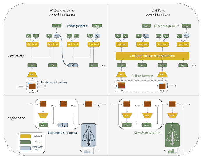
Figure 1: Comparison between the UniZero and MuZero-style architectures during training and inference phases. Left: In the MuZero-style architecture, the recursively unrolled latent representation $s^{k}_{t}$ is tightly coupled with historical information (entanglement). During training, it solely utilizes the initial observation of the sequence, resulting in under-utilization. During inference, the recursively predicted latent representation $s^{k}_{t-k}$ is used as the root node in MCTS, potentially causing inaccuracies due to compound errors, especially in scenarios requiring long-term dependencies. Right: UniZero adopts a transformer-based latent world model that explicitly disentangles the latent states from implicit latent history and utilizes all observations during the training phase. For inference, the directly encoded latent state $z_{t}$ is employed as the root node. Supported by a more complete and fully accessible context $M=(z_{t-H_{\text{infer}}},a_{t-H_{\text{infer}}},\dots,z_{t},a_{t})$, this approach enhances the accuracy of predictions and facilitates more effective long-term planning within the latent space.

In this section, we begin by analyzing the two main limitations of MuZero-style architectures, as discussed in Section 3.1, especially in their ability to handle tasks that require capturing long-term dependencies. To address these limitations, in Section 3.2, we introduce a novel approach termed UniZero, which is fundamentally a transformer-based latent world model. We provide a comprehensive description of its architectural design, along with the joint optimization procedure for both the model and the policy. In Section 3.3, we explore how to conduct efficient MCTS from a long-term perspective within the learned latent space. For more details on the algorithm’s implementation, please refer to Appendix B.

3.1 Main Limitations in MuZero-style Architectures

As illustrated in Figure 1, during the training phase, MuZero-style architectures utilize the initial observation $o_{t}$ (which may consist of stacked frames) and the entire sequence of actions as their input (actions omitted when context is clear). This approach results in the under-utilization of trajectory data, particularly when dealing with long trajectory sequences or scenarios requiring long-term dependencies. Moreover, MuZero employs dynamics networks to unroll several hypothetical steps during training, i.e., $\hat{r}^{k},s^{k}=g_{\theta}(s^{k-1},a^{k-1})$, as illustrated by the light blue data in Figure 1. Consequently, the recursively unrolled latent representation $s^{k}_{t}$ is tightly coupled with historical information, a phenomenon we refer to as entanglement. This entanglement is incompatible with the SSL loss, as discussed later. During inference, the latent representation encoded from the current observation $o_{t}$ (without historical information) is used as the root node in MCTS. While this design is effective in MDPs, we suspect it will fail in partially observable scenarios due to the lack of historical information. One simple extension is to instead use the recursively predicted latent representation $s^{k}_{t-k}$ as the root node. However, this method potentially introduces inaccuracies due to compounded errors, leading to suboptimal performance.

To empirically analyze the impact of these limitations on capturing long-term dependencies, we propose four variants of the MuZero-style algorithm and compare them with our UniZero approach:

• (Original) MuZero: This method does not utilize any self-supervised regularization. During inference, the root state $z_{t}$ is generated by encoding the current observation $o_{t}$ through the encoder.

• MuZero w/ SSL: As discussed in Section 2, to enhance sample efficiency, this variant integrates an auxiliary self-supervised regularization efficientzero into MuZero’s training objective. However, we argue that imposing this regularization loss might cause the predicted latent representation $s^{k}_{t-k}$ to rely excessively on the observation $o_{t}$ from a single timestep. This dependency could inadvertently diminish the importance of more extensive historical data. Thus, this variant seems primarily suitable for MDP tasks that align with such a design.

• MuZero w/ Context: This variant retains the same training settings as MuZero but diverges during inference by employing a $k$-step recursively predicted latent representation $s^{k}_{t-k}$ at the root node. Due to the presence of compound errors mbpo from recurrent predictions, the context at the root node is inaccurate, leading to prediction errors in the MCTS process. We refer to the issue of significant prediction errors and poor performance caused by partially accessible context as the phenomenon of incomplete context.

• UniZero: Our proposed UniZero (depicted on the right side of Figure 1) disentangles latent states $z_{t}$ from the implicit latent history using a transformer-based world model. This architecture enables the model to leverage the entire trajectory during training while ensuring the prediction of the next latent state $z_{t}$ at each timestep. During inference, UniZero preserves a relatively complete context within the most recent $H_{\text{infer}}$ steps by utilizing the Key-Value (KV) cache mechanism. This approach both enriches the learning signals with self-supervised regularization and maintains long-term dependencies.

• UniZero (RNN): This variant retains similar training settings as UniZero but employs a GRU GRU backbone. During the inference phase, the hidden state of the GRU is reset and cleared every $H_{\text{infer}}$ steps. Due to the recurrent mechanism and the limited memory length of the GRU, it also experiences the phenomenon of incomplete context. For more details, please refer to 5.

Table 1: Qualitative Comparison of Different Variants. MuZero utilizes only the first observation as input during training. MuZero w/ SSL incorporates a state regularization loss for latent representation, which is effective in MDP tasks. MuZero w/ Context and UniZero (RNN) both suffer from performance issues due to their reliance on recurrent mechanisms for historical information, resulting in partially accessible contexts. In contrast, UniZero, with its transformer-based architecture, disentangles latent states from the implicit latent history, leveraging the full observation sequence during training and ensuring a more complete and fully accessible context.

Algorithm	Disentanglement	Obs. Full Utilization	State Regularization	Context Access
MuZero	$\times$	$\times$	$\times$	$\times$
MuZero w/ SSL	$\times$	$\times$	$\checkmark$	$\times$
MuZero w/ Context	$\times$	$\times$	$\times$	partially accessible
UniZero (RNN)	$\checkmark$	$\checkmark$	$\checkmark$	partially accessible
UniZero	$\checkmark$	$\checkmark$	$\checkmark$	fully accessible

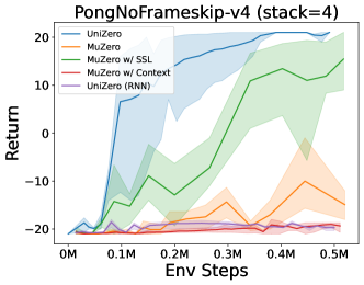
Figure 2: Performance comparison of UniZero and MuZero variants in Pong under approximate MDP and POMDP settings. Left: MDP setting. Right: POMDP setting. In both scenarios, UniZero consistently outperforms the other approaches, demonstrating the robustness and versatility of our architecture. MuZero w/ SSL shows good sample efficiency in the MDP setting but fails to converge in the POMDP setting due to entanglement issues. MuZero w/ Context and UniZero (RNN) struggle to learn effectively in both settings due to prediction errors arising from the incomplete context.

For comparison, Table 1 outlines the qualitative differences among these variants. Figure 2 illustrates their performance disparities in Pong under frame_stack=4 and frame_stack=1 settings, which approximately correspond to MDP and POMDP scenarios, as referenced in drqn . In the stack4 scenario, MuZero w/ SSL demonstrates good sample efficiency due to the rich learning signals provided by the auxiliary self-supervised regularization loss. However, in the stack1 setting, MuZero w/ SSL fails to converge within 500k environment steps, primarily due to issues related to the previously discussed entanglement design. Meanwhile, both MuZero w/ Context and MuZero w/ Context (RNN) face challenges in learning due to prediction errors arising from the incomplete context phenomenon. For MuZero w/ Context, these errors originate from its recurrently predicted latent representations, whereas for MuZero w/ Context (RNN), they stem from its recurrent hidden state of GRU. In both scenarios, UniZero outperforms the other variants, verifying its robustness and versatility.

3.2 Scalable Latent World Models

Building on the above insights, we introduce the UniZero method to address the challenges posed by the entanglement of latent representations with historical information and the under-utilization of trajectory data. In this subsection, we will outline the architecture of our method and provide detailed descriptions of the training procedures for the joint optimization of the model and the policy.

3.2.1 Transformer-based Latent World Models

Architecture. As depicted in the top right of Figure 1, UniZero comprises four principal components: the encoder $h_{\theta}$, the transformer backbone, the dynamics network $g_{\theta}$, and the decision network $f_{\theta}$. It is worth noting that in the following discussion, the transformer backbone might be implicitly incorporated within the last two networks. Formally, at each time step $t$, the environmental observations and actions are denoted by $o_{t}$ and $a_{t}$, respectively. For simplicity, $a_{t}$ may also represent the action embedding obtained via a lookup in a learned embedding table. We denote the latent states in UniZero by $z_{t}$, the predicted subsequent latent state by $\hat{z}_{t+1}$, and the predicted reward by $\hat{r}_{t}$. Furthermore, the policy (typically represented by action logits) and state value are denoted by $p_{t}$ and $v_{t}$, respectively, which are crucial for guiding the MCTS procedure towards regularized policy optimization mcts_optimization . In summary, the world model of UniZero $\mathcal{W}$ encapsulates the following parts:

$$\begin{array}[]{lll}&\text{encoder: }z_{t}=\text{h}_{\theta}\left(o_{t}\right)\color[rgb]{.5,.5,.5}{\vartriangleright\text{Maps observations to their latent states}}\\ &\text{\color[rgb]{0,0,1}{dynamics network}: }\quad\hat{z}_{t+1},\hat{r}_{t}=g_{\theta}\left(z_{\leq t},a_{\leq t}\right)\color[rgb]{.5,.5,.5}{\vartriangleright\text{Models latent dynamics and reward}}\\ &\text{\color[rgb]{1,0,0}{decision network}: }\quad p_{t},v_{t}=f_{\theta}\left(z_{\leq t},a_{\leq{t-1}}\right)\color[rgb]{.5,.5,.5}{\vartriangleright\text{Predicts policy and value}}\end{array}$$ (2)

Training. We categorize a single time step into two distinct tokens: the latent state and the action. For details about data pre-processing and tokenizers, please refer to Appendix 2. UniZero’s dynamic network is designed to predict the subsequent latent state and reward conditioned on the previous latent states and actions up to time step $t$: $(z_{\leq t},a_{\leq t})$. Concurrently, the decision network is tailored to predict the decision-relevant quantities (policy and state-value) based on the previous latent states and actions up to time steps $t$ and $t-1$: $(z_{\leq t},a_{\leq t-1})$. In MuZero-style approaches, which rely solely on the initial observation, the k-th latent representation $s_{t}^{k}$ is recursively inferred through the dynamic network. UniZero distinguishes itself with a transformer backbone network adept at learning an implicit latent history $h_{t}=\{h_{t}^{z},h_{t}^{z,a}\}$ at each time step. This innovative architecture enables UniZero to overcome the two aforementioned limitations of MuZero-style algorithms by explicitly separating the latent state $z_{t}$ from the implicit latent history $h_{t}$. Please note that we do not employ a decoder to reconstruct $z_{t}$ into $\hat{o}_{t}$. Although reconstruction is a common technique in prior research dreamerv3 to shape representations, our empirical findings from the experiments (see Section 4.4) show that omitting this decoding loss does not diminish performance. This observation supports our hypothesis that learned latent states only need to capture information relevant to decision-making, thereby making reconstruction unnecessary for decision tasks.

Inference. During inference, UniZero can leverage both the long-term memory preserved in KV Cache and encoded information from the current observation. The latent world model can generate more accurate internal predictions, which in turn serves as the root/internal node for tree search. The synergy between these components significantly boost the efficiency and scalability of UniZero.

3.2.2 Joint Optimization of Model and Policy

In this paper, our primary focus is on online reinforcement learning settings. Algorithm 1 presents the pseudo-code for the entire training pipeline. In this subsection, we will present the core process of joint optimization of the model and policy (behaviour). UniZero maintains a replay buffer $\mathcal{B}$ that stores trajectories $\{o_{t},a_{t},r_{t},o_{t+1},\pi_{t}\}$ (where $\pi_{t}$ is the MCTS improved policy induced in Section 3.3) and iteratively performs the following two steps:

1. Experience Collection: Collect experiences into the replay buffer $\mathcal{B}$ by interacting with the environment. Notably, the agent employs a policy derived from MCTS, which operates within the learned latent space.

2. Model and Policy Joint Update: Concurrent with data collection, UniZero performs joint updates on the decision-oriented world model, including the policy and the value functions, using data sampled from $\mathcal{B}$.

The joint optimization objective for the model-policy can be written as:

$$\begin{split}\mathcal{L}_{\text{UniZero}}(\theta)\doteq\mathop{\mathbb{E}}_{(o_{t},a_{t},r_{t},o_{t+1},\pi_{t})_{0}^{H-1}\sim\mathcal{B}}\Big{[}\sum_{t=0}^{H-1}\Big{(}&\color[rgb]{0,0,1}{\beta_{z}}\color[rgb]{0,0,1}{\underbrace{\color[rgb]{0,0,0}{\|\hat{z}_{t+1}-\operatorname{sg}(\bar{h}(o_{t+1}))\|^{2}_{2}}}_{\text{next-latent prediction}}}\color[rgb]{0,0,0}\color[rgb]{0,0,1}{\beta_{r}}\color[rgb]{0,0,1}{\underbrace{\color[rgb]{0,0,0}{\operatorname{CE}(\hat{r}_{t},r_{t})}}_{\text{reward prediction}}}\\ +&\color[rgb]{1,0,0}{\beta_{p}}\color[rgb]{1,0,0}{\underbrace{\color[rgb]{0,0,0}{\operatorname{CE}({p}_{t},\pi_{t})}}_{\text{policy prediction}}}\color[rgb]{0,0,0}\color[rgb]{1,0,0}{\beta_{v}}\color[rgb]{1,0,0}{\underbrace{\color[rgb]{0,0,0}{\operatorname{CE}({v}_{t},\hat{v}_{t})}}_{\text{value prediction}}}\color[rgb]{0,0,0}{\Big{)}\Big{]}}\end{split}$$ (3)

Note that we also maintain a soft target world model dqn $\bar{\mathcal{W}}=(\bar{h}_{\theta},\bar{g}_{\theta},\bar{f}_{\theta})$, which is an exponential moving average of current world model $\mathcal{W}$ 2. In Equation 3, $H$ is the training context length, $\operatorname{sg}$ is the stop-grad operator, $\operatorname{CE}$ denotes cross-entropy loss function, $\bar{h}(o_{t+1})=\bar{z}_{t+1}$ is the target latent state generated by the target encoder $\bar{h}_{\theta}$, and $\hat{v}_{t}$ signifies the bootstrapped $n$-step TD target: $\hat{v}_{t}=\sum_{k=0}^{n-1}\{\gamma^{k}r_{t+k}\}+\gamma^{n}\bar{f}_{\theta}\left(z_{\leq t},a_{\leq{t-1}}\right).$ As the magnitudes of rewards across different tasks can vary greatly, UniZero adopts reward and value predictions as discrete regression problems discrete_regression , and optimizes by minimizing the cross-entropy loss. $\pi_{t}$ represents the improved policy through MCTS shown in Section 3.3. We optimize the dynamics network to predict $\pi_{t}$, essentially seems a policy distillation process. Compared to policy gradient methods storm ; dreamer ; ppo , this approach potentially offers better stability muzero ; mcts_optimization . The coefficients $\color[rgb]{0,0,1}{\beta_{z},\beta_{r}},\color[rgb]{1,0,0}{\beta_{p},\beta_{v}}$ are constant coefficients used to balance different loss items. Inspired by tdmpc2 , UniZero has adopted the SimNorm technique, which is implemented after the final layer of the encoder and the last component of the dynamics network that predicts the next latent state. Essentially, this involves applying a L1 norm constraint to regularize the latent state space. As detailed in Section 4.4, latent normalization has been empirically proven to be crucial for enhancing the stability and robustness of training.

3.3 MCTS in Latent Space

RL agents need a memory $M$ to accurately model future in tasks that require long-term dependencies. To effectively implement this memory mechanism, as depicted in Figure 3 (for simplicity, we use $1$ as the starting timestep in this figure), we establish a KV Cache kvcache for the memory, denoted by: $KV_{M}=\{KV(z_{t-H},a_{t-H},\ldots,z_{t},a_{t})\}$. When the agent encounters a new observation $o_{t}$ and needs to make a decision, it first utilizes the encoder to transform this observation into the corresponding latent state $z_{t}$, which serves as the root node of the search tree. By querying the KV Cache, the keys and values from the recent memory $(z_{t-H_{\text{infer}}},a_{t-H_{\text{infer}}},\ldots,z_{t},a_{t})$ are retrieved for the transformer-based latent world model. This model recursively predicts the next latent state $\hat{z}_{t+1}$, the reward $\hat{r}_{t}$, the policy $p_{t}$, and the value $v_{t}$. The newly generated next latent state $\hat{z}_{t+1}$ functions as an internal node in the MCTS process. Subsequently, MCTS is executed within this latent space. Further details can be found in B.1.1. Upon completion of the search, the visit count set $\{N(z_{t},a_{t})\}$ is obtained at the root node $z_{t}$. These visit counts are then normalized to derive the improved policy $\pi_{t}$:

$$\pi_{t}=\frac{N(z_{t},a_{t})^{1/T}}{\sum_{b_{t}}N(z_{t},b_{t})^{1/T}}$$ (4)

Here, $T$ denotes the temperature, which modulates the extent of exploration ngu . Actions are then sampled from this distribution for interactions with the environment. After each interaction, we save the transition $(o_{t},a_{t},r_{t},d_{t},o_{t+1})$ along with the improved policy $\pi_{t}$ into the buffer, with the latter serving as the policy target in Eq. 3. By leveraging backward memory and forward search, UniZero demonstrates the potential to perform generalized and efficient long-term planning across a wide range of decision-making scenarios, as illustrated in Appendix D.2.

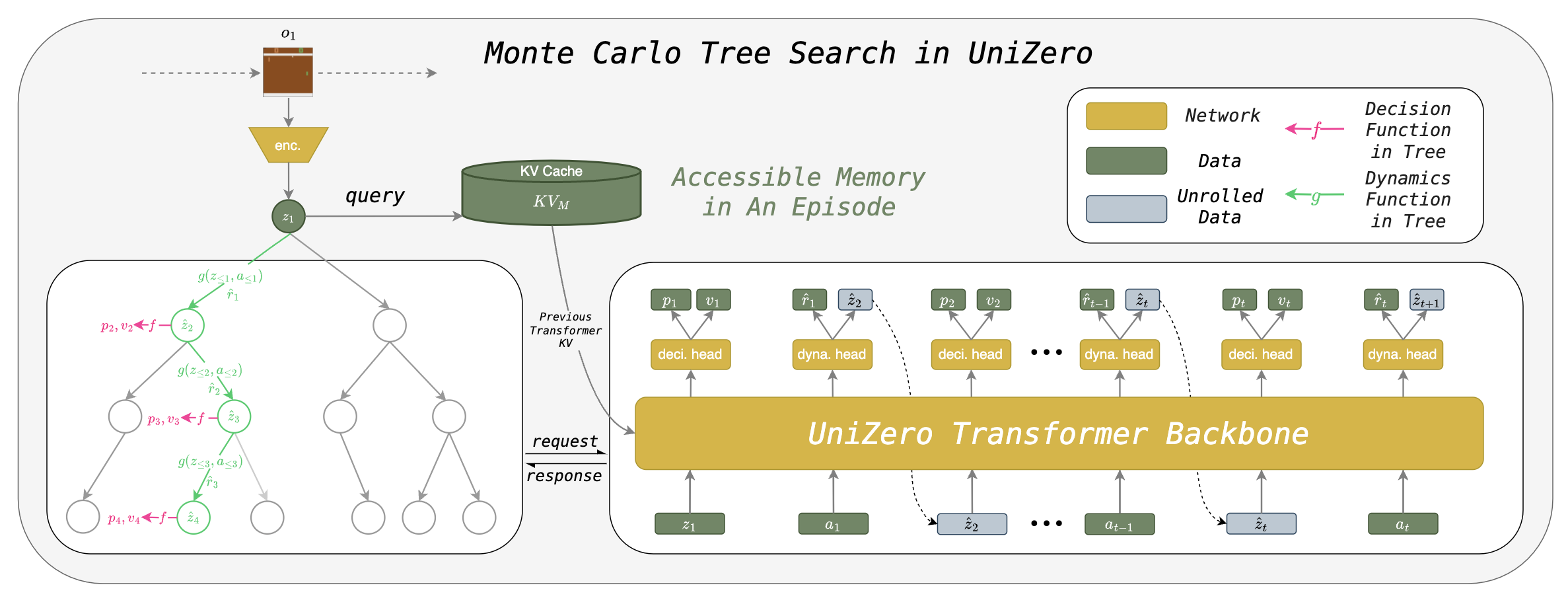
Figure 3: MCTS in the learned latent space. The process begins with a new observation $o_{1}$, which is encoded into a latent state $z_{1}$. This latent state serves as the root node for the MCTS. The previous keys and values of recent memory are retrieved from the transformer’s KV Cache $KV_{M}$. Subsequently, the search tree utilizes the world model to predict the next latent state $\hat{z}$ (which serves as an internal node), reward $\hat{r}$, policy $p$, and value $v$, conditioned on the retrieved KV, recursively. These predictions are then employed to conduct MCTS, ultimately resulting in an improved policy $\pi$.

4 Experiments

We evaluate the performance of UniZero across 26 distinct games using the Atari 100k benchmark simple (Section 4.2). Additionally, we perform a qualitative analysis of its long-term modeling capabilities using the long-term dependency benchmark, specifically the VisualMatch tasks, which necessitate extensive memory capacity (Section 4.3). To assess the impact of each component of UniZero, we conduct comprehensive ablation studies (Section 4.4) and a series of visual analyses (Appendix D.2). Due to its unified architecture and training paradigm, UniZero can seamlessly extend to a multi-task learning setup. Preliminary multi-task results on four Atari games in Appendix E validate the scalability and potential of UniZero in multi-task learning scenarios. Our implementations leverage the latest open-source MCTS framework, LightZero lightzero . For additional details, including specific environment settings, further experiments, and other implementation specifics, please refer to Appendices A, B, and C.1.

4.1 Experiments Setup

Environments. Introduced by SimPLe simple , the Atari 100k benchmark has been widely used in studies focusing on sample-efficient RL SPR . It provides a robust measure of the sample efficiency of various algorithms. In addition to this, our experiments also include the VisualMatch transformers_rl , designed to evaluate long-term memory capabilities. This benchmark is set in grid-world scenarios with exploration, distraction, and reward phases transformers_rl . More details about environments can be found in Appendix A.

Baselines. In the Atari 100k benchmark, we employed three baselines: MuZero w/ SSL (stack=4), MuZero w/ SSL (stack=1), and EfficientZero (stack=4), all the variants are re-implemented using LightZero. For brevity, "w/ SSL" may be occasionally omitted in subsequent mentions. For long-term dependency benchmark, our primary baselines are MuZero (stack=1) and the SAC-Discrete variant algorithm combined with the GPT gpt backbone as proposed in transformers_rl . In our analysis, we refer to the latter as SAC-GPT. As mentioned in Section 3.1, due to the inherent challenges of UniZero (RNN) in modeling long-term dependencies, which result in its poor performance, we did not consider it as our baseline. We plan to delve into a more in-depth analysis of UniZero (RNN) in future research. Additional details regarding experimental setups are available in Appendix C.1.

4.2 Atari

Categorization. It is crucial to recognize that in Atari environments, certain games behave as POMDPs when the input is a single frame. This means they rely on historical information to make optimal decisions, examples include Pong and Seaquest. Conversely, other environments function as MDPs, where optimal decisions can be made based solely on a single frame, such as MsPacman and Boxing. We categorize the former as POMDP-like tasks and the latter as MDP-like tasks drqn .

Results. In this subsection, we compare UniZero with MuZero and its variants across these four representative Atari environments in Figure 4. Results demonstrate that in POMDP-like tasks (e.g., Pong and Seaquest), MuZero (stack1) performs poorly due to the lack of necessary contextual information for decision-making. In contrast, UniZero (stack1) with only single-frame input achieves performance comparable to, or even surpassing, MuZero (stack4) and EfficientZero (stack4). In MDP-like tasks (e.g., MsPacman and Boxing), MuZero (stack1) performs similarly to MuZero (stack4), and UniZero’s performance is on par with both baselines. We report the complete results for 26 games on the Atari 100k benchmark in Appendix C.2, including additional model-based RL algorithms dreamerv3 ; iris ; storm as baselines. Overall, UniZero (stack1) outperforms MuZero (stack4) in 17 out of 26 games in the Atari 100k benchmark and demonstrates comparable performance in most of the remaining games. This reveals that UniZero is capable of modeling both short- and long-term dependencies simultaneously, demonstrating its versatility.

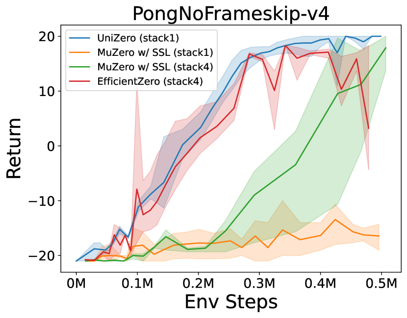
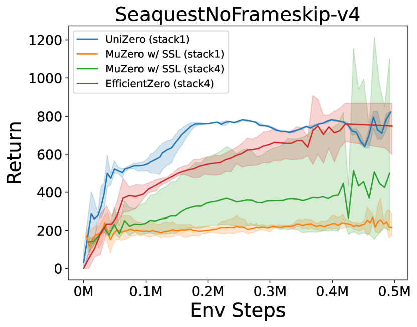
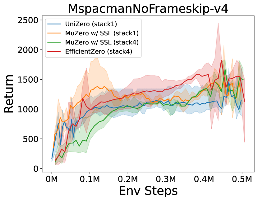
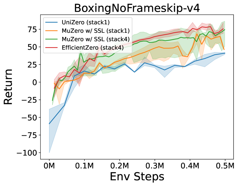
Figure 4: Performance comparison on representative Atari Games. In POMDP-like tasks (e.g., Pong, Seaquest), UniZero outperforms MuZero (stack1) and either matches or exceeds the performance of MuZero (stack4) and EfficientZero (stack4). In MDP-like tasks (e.g., MsPacman, Boxing), MuZero (stack1) performs similarly to MuZero (stack4), and UniZero matches both, demonstrating UniZero’s versatility in modeling both short- and long-term dependencies. The solid line represents the mean of 5 runs; the shaded areas are 95% confidence intervals.

4.3 Long-Term Dependency Benchmark

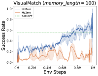
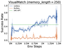
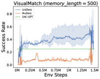
Figure 5: Performance comparison on VisualMatch with increased memory lengths. MuZero consistently underperformed across all tasks, primarily due to insufficient context information. The performance of SAC-GPT significantly deteriorated as the memory length increased. In contrast, UniZero maintained a high success rate even with extended memory lengths, owing to its robust long-term dependency capabilities.

In Figure 5, we compare the performance of UniZero and MuZero on the VisualMatch benchmark, which requires long-term memory. The green horizontal dashed line represents the final success rate of SAC-GPT transformers_rl after training on 3 million environment steps. Due to the lack of context, MuZero performs poorly across all tasks, and the performance of SAC-GPT significantly declines as the memory length increases. In contrast, UniZero maintains a high success rate as the memory length increases, which supports our analysis in Section 3.1.

4.4 Ablation Study

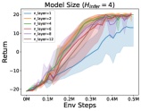
(a)

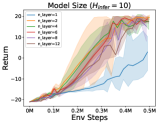
(b)

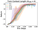
(c)

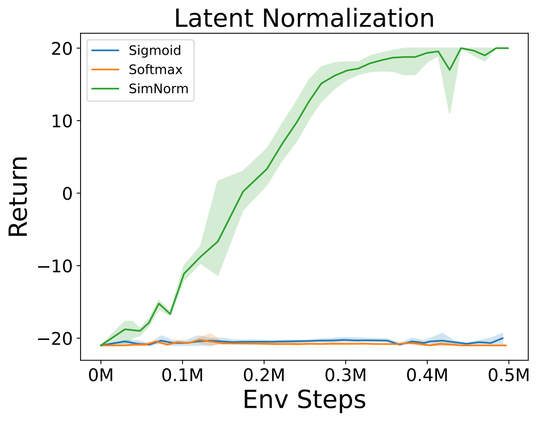
(d)

(e)

Figure 6: Ablation study in Pong validates the efficiency of key design choices in UniZero. (a-c) UniZero demonstrates robust performance with increasing model size and training context length. (d) Proper latent space normalization (e.g. SimNorm) is essential for ensuring training stability. (e) For decision-making tasks, decode regularization has a negligible impact. The solid line represents the mean of 3 runs; the shaded areas are 95% confidence intervals.

This subsection and Appendix D evaluate the effectiveness of the key design choices in UniZero:

• Model Size (n_layer) across different Inference Context Lengths ($H_{\text{infer}}=4/8$) with fixed Train Context Length ($H=8$).

• Train Context Length ($H$) with fixed Inference Context Length ($H_{\text{infer}}=4$).

• Latent Normalization: Comparison of normalization techniques that employed in the latent state, including SimNorm (default), Softmax and Sigmoid.

• Decode Regularization: Integrate a decoder on top of the latent state: $\hat{o}_{t}=d_{\theta}(z_{t})$. Followed by an additional training objective: $\mathcal{L}_{\text{decode\_reg}}=\|o_{t}-d_{\theta}(z_{t})\|_{1}+\mathcal{L}_{\text{perceptual}}(o_{t},d_{\theta}(z_{t})),\text{where}\ z_{t}=h_{\theta}(o_{t})$. The first term is the reconstruction loss, and the second term is the perceptual loss transformers_rl .

Figure 6 presents a series of ablation results on Pong while the ablation results on VisualMatch and related detail settings are included in Appendix D. Based on these experiment results, we can conclude the following key findings: (1) Performance at $H_{\text{infer}}=4$ consistently surpasses $H_{\text{infer}}=8$, regardless of the model size. A shorter context is sufficient for tasks like Pong. For VisualMatch, context length should match the episode length to retain target color memory. This suggests that we could dynamically select the inference context length $H_{\text{infer}}$ based on the long-term dependency requirements of the task, which will be addressed in our future work. (2) Performance generally improves with longer Train Context Length ($H$), suggesting that forecasting longer future aids representation learning, consistency with findings in brain . (3) SimNorm yields the best results compared with Softmax and Sigmoid. It emphasizes the critical role of proper latent space normalization in maintaining stability. SimNorm introduces natural sparsity by constraining the L1 norm of the latent state to a fixed constant, thereby ensuring stable gradient magnitudes. (4) In both Pong and VisualMatch, Decode Regularization has a negligible impact, supporting our analysis that decision-relevant information in latent states is more critical than observation reconstruction. More detailed visual analyses and preliminary multi-task results can be found in Appendix D.2 and E.

5 Related Work

MCTS-based RL. Algorithms like AlphaGo alphago and AlphaZero alphazero , which combine MCTS with deep neural networks, have significantly advanced board game AI. Extensions such as MuZero muzero , Sampled MuZero sampledmuzero , and Stochastic MuZero stochastic have adapted this framework for environments with complex action spaces and stochastic dynamics. EfficientZero efficientzero and GumbelMuZero gumbel have further increased the algorithm’s sample efficiency. MuZero Unplugged unplugged ; rezero introduced reanalyze techniques, enhancing performance in both online and offline settings. LightZero lightzero addresses real-world challenges and introduces a comprehensive open-source MCTS+RL benchmark. Studies like RAP rap and SearchFormer searchformer have applied MCTS to enhance the reasoning capabilities of language models gpt3 . We analyze the challenges MuZero faces in modeling long-term dependencies in POMDPs and propose a transformer-based latent world model to address these challenges.

World Models. The concept of world models, first proposed in world_models , enables agents to predict and plan future states by learning a compressed spatiotemporal representation. Subsequent research dreamerv2 ; dreamerv3 ; dreamer ; iris ; twm ; storm ; tdmpc ; tdmpc2 ; muzero ; efficientzero ; visualizing_muzero has enhanced world models in both architecture and training paradigms. These studies generally follow three main routes based on training paradigms: (1) The Dreamer series dreamerv2 ; dreamerv3 ; dreamer adopts an actor-critic paradigm, optimizing policy and value functions based on internally simulated predictions. Note that the model and behavior learning in this series are structured in a two-stage manner. Building on this, iris ; twm ; storm leverage Transformer-based architectures to enhance sequential data processing, achieving significant sample efficiency and robustness. (2) The TD-MPC series tdmpc ; tdmpc2 demonstrates substantial performance gains in large-scale tasks by learning policies through local trajectory optimization within the latent space of the learned world model, specifically utilizing the model predictive control algorithm mpc . The model and behavior learning in this series also follow a two-stage structure. (3) Research stemming from MuZero muzero ; efficientzero ; visualizing_muzero , grounded in the value equivalence principle value_equivalence , achieves joint optimization of the world model and policy MoM ; ALM and employs MCTS for policy improvement. Despite these advancements, the effective integration of these approaches remains underexplored. In our paper, we provide a preliminary investigation into integrating scalable architectures and joint model-policy optimization training paradigms. A detailed qualitative comparison is presented in Appendix 9.

6 Conclusion and Future work

In this paper, we explore the efficiency of MuZero-style algorithms in environments that require long-term dependencies. Through qualitative analyses, we identify two key limitations in MuZero: under-utilization and entanglement. To address these issues and extend MuZero’s applicability, we introduce UniZero, which integrates a transformer-based latent world model and MCTS. Our experimental results and visualizations demonstrate UniZero’s efficacy and scalability across various environments. Our work currently employs the classic transformer, presenting opportunities for developing domain-specific techniques for decision-making scenarios, such as attention optimizations flash_attn ; gqa . Additionally, UniZero’s potential as a foundational model for large-scale multi-task learning and continuous control remains an open area for future research, which we are committed to exploring.

7 Acknowledgements

We extend our gratitude to several team-members of the Shanghai AI Laboratory and SenseTime for their invaluable assistance, support, and feedback on this paper and the associated codebase. In particular, we would like to thank Chunyu Xuan, Ming Zhang, and Shuai Hu for their insightful and inspiring discussions at the inception of this project.

Appendix A Environment Details

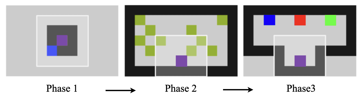
Figure 7: The Long-Term Dependency Benchmark, VisualMatch, organizes each task into 3 phases: Exploration, Distraction, Reward. In this benchmark, the duration (steps) of Phase 2 varies (denoted as memory_length), while the durations of the other phases remain fixed. The agent, depicted in purple, has a limited field of view, observing only nearby grids within white borders, and is unable to cross walls shown in black. This setup creates a POMDP environment. The agent is presented with a randomized target color (blue in this case) during Phase 1. In Phase 2, the environment introduces random distractions, such as green apples. Finally, in Phase 3, the agent must navigate to the grid corresponding to the previously observed target color. As the memory length increases, the ability to model long-term dependencies in agents becomes increasingly critical for solving tasks.

A.1 Atari 100k Benchmark

Introduced by SimPLe [45], the Atari 100k benchmark is widely used in sample-efficient reinforcement learning research. This benchmark includes 26 diverse image-input Atari games with discrete action dimensions of up to 18, providing a diverse and robust measure of algorithm performance. Agents interact for 100,000 steps per game, equivalent to 400k environment frames, with frame skipping every 4 frames.

A.2 Long-Term Dependency Benchmark

This benchmark, specifically Visual Match, is designed to test long-term memory with adjustable memory lengths. As illustrated in Figure 7, these tasks are structured as grid-world scenarios and are divided into three phases: exploration, distraction, and reward.

• Exploration Phase: The agent observes a room with a random RGB color.

• Distraction Phase: Randomly appearing apples, served as random distractions.

• Reward Phase: The agent selects a block that matches the initial room color.

In our experiments, Phase 1 is set to 1 step, and Phase 3 is set to 15 steps. The target colors in Phase 3 are randomly chosen from three predefined colors: blue, red, and green.

Our setup differs from [2] primarily in the reward structure:

• Collecting apples in Phase 2 yields zero reward.

• A reward of 1 is given only upon goal completion in Phase 3, making the environment one of entirely sparse rewards.

• Additionally, in Visual Match, Phase 1 is set to 1 step, compared to 15 steps in [2].

The Visual Match task is designed to evaluate an agent’s ability to manage long-term dependencies in decision-making processes. In this task, the agent must remember a specific color encountered during the exploration phase and later identify the corresponding grid in the reward phase, thus testing its long-term memory. The task features sparse rewards, with the agent earning a point only upon successfully completing the target. Additionally, the environment is partially observable, limiting the agent’s field of view to a 5x5 grid area at each step. This restriction compels the agent to make decisions based on incomplete information, mirroring many real-world scenarios.

Appendix B Implementation Details

B.1 Algorithm Details

Procedure training_loop():

       for train_iterations do

             Create a Key-Value Cache for the memory: $KV_{M}=\{\}$

             collect_experience(collect_steps)

             for world_model_iterations do

                   update_world_model()

                  

            // Due to the variations in the parameters of the world model. We need clear the old Key-Value Cache

             Clear the Key-Value Cache: $KV_{M}=\{\}$

            

      

Procedure collect_experience($n$):

       $o_{0}\leftarrow\texttt{env.reset()}$

       for $t=0$ to $n-1$ do

             ${z}_{t}\leftarrow h_{\theta}(o_{t})$

             Sample $a_{t}\sim\pi_{t}=\pi(a_{t}|{z}_{t})$, which is obtained through MCTS(${z}_{t}$, $KV_{M}$, $\mathcal{W}$)

             Add the latest Key-Value Cache $KV(z_{t},a_{t})$ to $KV_{M}$

             $o_{t+1},r_{t},d_{t}\leftarrow\texttt{env.step(}a_{t}\texttt{)}$

             if $d_{t}=1$ then

                   $o_{t+1}\leftarrow\texttt{env.reset()}$

                  

            

      $\mathcal{B}\leftarrow\mathcal{B}\cup\{o_{t},a_{t},r_{t},o_{t+1},\pi_{t}\}_{t=0}^{n-1}$

      

Procedure update_world_model():

       Sample a mini-batch of sequences $\{(o_{t},a_{t},r_{t},o_{t+1},\pi_{t})_{t=i}^{i+H-1}\}\sim\mathcal{B}$ // where $H$ is the training context length.

       Compute target TD-value $\hat{v}_{t},$ and target next latent state $\bar{z}_{t+1}$ according to the target world model $\bar{\mathcal{W}}$

       Optimize the world model and policy jointly according to Equation 3

      

Procedure MCTS(${z}_{t}$, $KV_{M}$, $\mathcal{W},sim$):

       // The following process will repeat $sim$ iterations/simulations, where $i$ represents the current simulation step.

       Require : $N_{i}(\hat{z},a)$, $Q_{i}(\hat{z},a)$, $P_{i}(\hat{z},a)$, $R_{i}(\hat{z},a)$, $Z_{i}(\hat{z},a)$

      

      Initialize $\text{root node}\leftarrow z_{t}$

       repeat

             $a^{*}\leftarrow\operatorname{PUCT}(Q,P,N)$ as in Equation 5

            

      until $N_{i}(\hat{z}_{t}^{l},a^{l})=0$

      Evaluate the leaf root node $\hat{z}_{t}^{l}$ using $\mathcal{W}$: $p_{t}^{l},v_{t}^{l}\leftarrow f_{\theta}(\hat{z}_{t}^{l},KV_{M})$, $\hat{z}_{t}^{l+1},\hat{r}_{t}^{l}\leftarrow g_{\theta}(\hat{z}_{t}^{l},a^{l},KV_{M})$ and stored the dynamics and decision quantities into the corresponding tables $R_{i}(\hat{z},a)$, $Z_{i}(\hat{z},a)$, $P_{i}(\hat{z},a)$

       for each $\hat{z}$ along the search path do

             $Q_{i+1}(\hat{z},a)=\frac{N_{i}(\hat{z},a)\cdot Q_{i}(\hat{z},a)+\hat{v}(\hat{z})}{N_{i}(\hat{z},a)+1}$

             $N_{i+1}(\hat{z},a)=N_{i}(\hat{z},a)+1$

            

      return $\pi_{t}=\texttt{Normalization}(\{N_{i+1}(z_{t},a_{t})|a_{t}\in\mathcal{A}\})$

      

Algorithm 1 UniZero

Here, we present the complete training pipeline of UniZero in Algorithm 1. The training_loop of the UniZero algorithm consists of two primary procedures:

1. collect_experience: This procedure gathers experiences (trajectories) $\{o_{t},a_{t},r_{t},d_{t}\}$ and the improved policy $\pi_{t}$ derived from Monte Carlo Tree Search (MCTS) into the replay buffer $\mathcal{B}$. The agent interacts with the environment by sampling actions $a_{t}$ from the MCTS policy $\pi_{t}$, which is generated by performing MCTS in the learned latent space.

2. update_world_model: This procedure jointly optimizes the world model and the policy. UniZero updates the decision-oriented world model, policy, and value using samples from $\mathcal{B}$.

collect_steps in Algorithm 1 is defined as num_episodes_each_collect $\times$ episode_length. In our experiments, num_episodes_each_collect is typically set to 8. The parameter world_model_iterations in Algorithm 1 is calculated as collect_steps $\times$ replay_ratio (the ratio between collected environment steps and model training steps) [59]. In our experiments, replay_ratio is usually set to 0.25.

B.1.1 MCTS in the Learned Latent Space

As delineated in Algorithm 1, the MCTS procedure [10] within the learned latent space comprises 3 phases in each simulation step $i$. The total iterations/simulation steps in a single search process is denoted as $sim$:

• Selection: Each simulation initiates from the internal root state $z_{t}$, which is the latent state encoded by the encoder $h_{\theta}$ given the current observation $o_{t}$. The simulation proceeds until it reaches a leaf node $\hat{z}_{t}^{l}$, where $t$ signifies the search root node is at timestep $t$, and $l$ indicates it’s a the leaf node. For each hypothetical timestep $k=1,...,l$ of the simulation, actions are chosen based on the Predictor Upper Confidence Bound applied on Trees (PUCT) [60] formula:

  $$a^{k,*}=\arg\max_{a}\left[Q(\hat{z},a)+P(\hat{z},a)\frac{\sqrt{\sum_{b}N(\hat{z},b)}}{1+N(\hat{z},a)}\left(c_{1}+\log\left(\frac{\sum_{b}N(\hat{z},b)+c_{2}+1}{c_{2}}\right)\right)\right]$$ (5)

  where $N$ represents the visit count, $Q$ denotes the estimated average value, and $P$ is the policy’s prior probability. The constants $c_{1}$ and $c_{2}$ regulate the relative weight of $P$ and $Q$. For the specific values, please refer to Table 6. For $k<l$, the next state and reward are retrieved from the latent state transition and reward table as $\hat{z}^{k+1}=S\left(\hat{z}^{k},a^{k}\right)$ and $\hat{r}^{k}=R\left(\hat{z}^{k},a^{k}\right)$.

• Expansion: At the final timestep $l$ of the simulation $i$, the predicted reward and latent state are computed by the dynamics network $g_{\theta}$: $\hat{r}^{l},\hat{z}^{l+1}=g_{\theta}\left(\hat{z}^{l},a^{l},KV_{M}\right)$, and stored in the corresponding tables, $R\left(\hat{z}^{l},a^{l}\right)=r^{l}$ and $S\left(\hat{z}^{l},a^{l}\right)=\hat{z}^{l+1}$. The policy and value are computed by the decision network $f_{\theta}$: $p^{l},v^{l}=f_{\theta}\left(\hat{z}^{l},KV_{M}\right)$. A new internal node, corresponding to state $z^{l}$, is added to the search tree. Each edge $\left(\hat{z}^{l},a\right)$ from the newly expanded node is initialized to $\{N\left(s^{l},a\right)=0,Q\left(s^{l},a\right)=0,P\left(s^{l},a\right)=p^{l}\}$.

• Backup: At the end of the simulation, the statistics along the simulation path are updated. The estimated cumulative reward at step $k$ is calculated based on $\bar{v}^{l}$, i.e., an $(l-k)$-TD bootstrapped value:

  $$\hat{v}^{k}=\sum_{i=0}^{l-1-k}\gamma^{i}\hat{r}_{k+1+i}+\gamma^{l-k}\bar{v}^{l}$$ (6)

  where $\hat{r}$ are predicted rewards obtained from the dynamics network $g_{\theta}$, and $\bar{v}$ are obtained from the target decision network $\bar{f}_{\theta}$. Subsequently, $Q$ and $N$ are updated along the search path, following the equations in the MCTS procedure described in 1.

Upon completion of the search, the visit counts $N(\hat{z},a)$ at the root node $z_{t}$ are normalized to derive the improved policy:

$$\pi_{t}=\mathcal{I}_{\pi}(a|z_{t})=\frac{N(z_{t},a)^{1/T}}{\sum_{b}N(z_{t},b)^{1/T}}$$ (7)

where $T$ is the temperature coefficient controlling exploration. Finally, an action is sampled from this distribution for interaction with the environment. UniZero leverages key-value (KV) caching and attention mechanisms to enhance backward memory capabilities and employs Monte Carlo Tree Search (MCTS) to improve forward planning efficiency. By integrating these two technological directions, UniZero significantly advances more general and efficient planning.

B.2 Architecture Details

Encoder. In the Atari 100k experiment, our observation encoder architecture principally follows the framework described in the LightZero paper [14], utilizing the convolutional networks. A notable modification in UniZero is the addition of a linear layer at the end, which maps the original three-dimensional features to a one-dimensional latent state of length 768 (denoted as latent state dim, $D$), facilitating input into the transformer backbone network. Additionally, we have incorporated a SimNorm operation, similar to the details described in the TD-MPC2 paper [7]. Let $V$ (=8 in all our experiments) be the dimensionality of each simplex $\mathbf{g}$, constructed from $L$ (= $D$ / $V$) partitions of $\mathbf{z}$. SimNorm applies the following transformation:

$$\mathbf{z}^{sim\_norm}\doteq\left[\mathbf{g}_{1},\dots,\mathbf{g}_{i},\dots,\mathbf{g}_{L}\right],\quad\mathbf{g}_{i}=\frac{e^{\mathbf{z}_{i:i+V}/\tau}}{\sum_{j=1}^{V}e^{\mathbf{z}_{i:i+V}/\tau}},$$ (8)

where $\mathbf{z}^{sim\_norm}$ is the simplicial embedding [61] of $\mathbf{z}$, $\left[\cdot\right]$ denotes concatenation, and $\tau>0$ is a temperature parameter that modulates the sparsity of the representation. We set $\tau$ to 1. As demonstrated in 4.4, SimNorm is crucial for the training stability of UniZero.

For the encoder used in the Long-Dependency Benchmark, we employed a similar conv. network architecture, with a latent state of length 64. Specifics can be found in the related table (see Table 2).

Dynamics Head and Decision Head. Both the dynamics head and the decision head utilize two-layer linear networks with GELU [62] activation functions. Specifically, the final layer’s output dimension for predicting value and reward corresponds to the support size (refer to B.3) [10, 41]. For predicting policy, the output dimension matches the action space size. For predicting the next latent state, the output dimension aligns with the latent state dimension, followed by an additional SimNorm normalization operation. In the context of Atari games, this dimension is set to 768, whereas for VisualMatch, it is configured to 64.

Table 2: Architecture of the encoder for VisualMatch. The size of the submodules is omitted and can be derived from the shape of the tensors. LeakyReLU refers to the leaky rectified linear units used for activation, while Linear represents a fully-connected layer. SimNorm [7] operations introduces natural sparsity by constraining the L1 norm of the latent state to a fixed constant, thereby ensuring stable gradient magnitudes. Conv denotes a CNN layer, characterized by $\text{kernel}=3$, $\text{stride}=1$, and $\text{padding}=1$. BN denotes the batch normalization layer.

Submodule	Output shape
Input image ($o_{t}$)	$3\times 5\times 5$
Conv1 + BN1 + LeakyReLU	$16\times 5\times 5$
Conv2 + BN2 + LeakyReLU	$32\times 5\times 5$
Conv3 + BN3 + LeakyReLU	$64\times 5\times 5$
AdaptiveAvgPool2d	$64\times 1\times 1$
Linear	$64$
SimNorm	$64$

Transformer Backbone. Our transformer backbone is based on the nanoGPT project, as detailed in Table 5. For each timestep input, UniZero processes two primary modalities. The first modality involves latent states derived from observations, normalized in the final layer using SimNorm, as discussed above. The second modality pertains to actions, which are converted into embeddings of equivalent dimensionality to the latent states via a learnable nn.Embedding layer. For continuous action spaces, these can alternatively be embedded using a learnable linear layer. Notably, rewards are not incorporated as inputs in our current framework. This choice is based on the rationale that rewards are determined by observations and actions, and thus do not add additional insight into the decision-making process. Furthermore, our approach does not employ a return-conditioned policy [23, 63], leaving the potential exploration of reward conditions to future work. Each timestep’s observed results and corresponding action embeddings are added with a learnable positional encoding, implemented through nn.Embedding, as shown in Table 3. While advanced encoding methods like rotary positional encoding [64] and innovate architectures of transformer [57] exist, their exploration is reserved for future studies. Detailed hyper-parameters can be found in Appendix B.3.

Table 3: Positional encoding module. $w_{1:H}$ is a learnable parameter matrix with shape $H\times D$, and $H$ refers to the sequence length and $D$ refers to the latent state dimension, 768 for the Atari, 64 for the VisualMatch.

Submodule	Output shape
Input ($(z_{1:H},a_{1:H})$)	$2H\times D$
Add ($(z_{1:H},a_{1:H})+w_{1:H}$)

Table 4: Details of Transformer block. $MHSA$ refers to multi-head self-attention and $FFN$ refers to feed-forward networks. Dropout mechanism can prevent over-fitting.

Submodule	Module alias	Output shape
Input features (label as $x_{1}$)	-	$2H\times D$
Multi-head self attention + Dropout($p$)	MHSA	$2H\times D$
Linear1 + Dropout($p$)
Residual (add $x_{1}$)
LN1 (label as $x_{2}$)
Linear2 + GELU	FFN	$2H\times D$
Linear3 + Dropout($p$)		$2H\times D$
Residual (add $x_{2}$)		$2H\times D$
LN2		$H\times D$

Table 5: Transformer-based latent world model $(p_{1:H},v_{1:H},\hat{z}_{1:H},\hat{r}_{1:H},h^{z}_{1:H},h^{z,a}_{1:H})=f_{\theta}(z_{1:H},a_{1:H})$. The hidden states $(h^{z}_{1:H},h^{z,a}_{1:H})$ in the final layer of the transformer are referred to as the implicit latent history. Positional encoding and Transformer block are explained in Table 3 and 4.

Submodule	Output shape
Input ($(z_{1:H},a_{1:H})$)	$2*H\times D$
Positional encoding
Transformer blocks $\times N$
(implicit) Latent history ($(h^{z}_{1:H},h^{z,a}_{1:H})$)
Decision head ($p_{1:H},v_{1:H}$)
Dynamic head ($\hat{z}_{1:H},\hat{r}_{1:H}$)

UniZero (RNN). This variant employs a training setup akin to UniZero but utilizes a GRU [38] as the backbone network. During training, all observations are utilized. During inference, the hidden state of the GRU is reset every $H_{\text{infer}}$ steps. The recursively predicted hidden state $h_{t}$ and observation embedding $z_{t}$ serve as the root node of the MCTS. The recursively predicted hidden state $h_{t}$ and predicted latent state $\hat{z}_{t}$ serve as the internal nodes. At the root node, due to the limited memory length of the GRU, the recurrent hidden state $h_{t}$ may not fully capture the historical information. At the internal nodes, the issue is exacerbated by the accumulation of errors, leading to inaccurate predictions and consequently limiting performance. For an illustration of the training process, please refer to Figure 8.

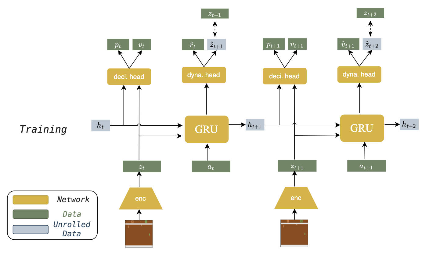
Figure 8: Training pipeline of UniZero (RNN). During training, all observations are utilized. The recursively predicted hidden state $h_{t}$ and observation embedding $z_{t}$ serve as the root node. The recursively predicted hidden state $h_{t}$ and predict latent state $\hat{z}_{t}$ serve as the internal nodes of MCTS. During inference, the GRU hidden state is reset every $H_{\text{infer}}$ steps. However, potential inaccuracies may arise from the recursively predicted hidden state $h_{t}$ due to the limited memory length of the GRU.

B.3 Hyperparameters

We use the same hyperparameters across all tasks, unless otherwise noted. Table 6 lists the key hyperparameters for UniZero, which mostly align with those in [14]. Table 7 shows the key hyperparameters for MuZero w/ SSL, MuZero w/ Context and UniZero (RNN). EfficientZero shares the similar key hyperparameters as MuZero w/ SSL, with an added LSTM [65] for predicting value_prefix, as specified in [14]. Note that in our reimplementation, to save computation time, reanalyze_ratio is set to 0.

Table 6: UniZero key hyperparameters. We use the same hyperparameters across all tasks other than specifically statement. For fair comparison, most hyperparameters are consistency with [14]. We use long-term denotes long-term dependency benchmark for simplicity.

Hyperparameter	Value
Planning
Number of simulations in MCTS ($sim$)	50
Inference Context Length ($H_{\text{infer}}$)	$4$ for Atari; memory_length+16 for long-term
Temperature	$0.25$
Dirichlet noise alpha	0.3
Dirichlet noise weight	0.25
$c_{1}$	1.25
$c_{2}$	19652
Env and Replay buffer
Capacity	$1,000,000$
Sampling	Uniform
Obs shape (Atari)	(3, 64, 64) for stack1, (4, 64, 64) for stack4
Obs shape ($textit{long-term}$)	(3, 5, 5)
Reward clipping	True (only for Atari)
Num of frames stacked	1 for stack1, 4 for stack4 (only for Atari)
Num of frames skip	4 (only for Atari)
Length of game segment	400 for Atari; memory_length+16 for long-term
Use data augmentation	False
Architecture
Latent state dim ($D$)	$768$ for Atari; $64$ for long-term
Num of heads in Transformer	$8$ for Atari; $4$ for long-term
Num of layers in Transformer ($N$)	$4$
Dropout in Transformer ($p$)	$0.1$
Activation	LeakyReLU in encoder, GELU in others
Number of reward/value bins	$101$
SimNorm dim ($V$)	$8$
SimNorm temperature ($\tau$)	$1$
Optimization
Train Context Length ($H$)	$10$
Replay ratio	$0.25$
Reanalyze ratio	0
Batch size	$64$
Optimizer	AdamW
Learning rate	$1\times 10^{-4}$
Next latent state loss coef.	$10$
Reward loss coef.	$1$
Policy loss coef.	$1$
Value loss coef.	$0.25$
Policy entropy coef.	$1\times 10^{-4}$
Weight decay	$10^{-4}$
Max gradient norm	5
Discount factor	0.997
Momentum of soft target network update	0.05
Frequency of hard target network update	100
TD steps	5

Table 7: Key hyperparameters for MuZero w/ SSL, MuZero w/ Context and UniZero (RNN).

Hyperparameter	Value
Planning
Number of simulations in MCTS ($sim$)	50
Inference Context Length ($H_{\text{infer}}$)	$0$ for MuZero w/ SSL, $4$ for MuZero w/ Context
Temperature	$0.25$
Dirichlet noise alpha	0.3
Dirichlet noise weight	0.25
$c_{1}$	1.25
$c_{2}$	19652
Env and Replay buffer
Capacity	$1,000,000$
Sampling	Uniform
Obs shape (Atari)	(3, 64, 64) for stack1, (4, 64, 64) for stack4
Obs shape ($textit{long-term}$)	(3, 5, 5)
Reward clipping	True (only for Atari)
Num of frames stacked	1 for stack1, 4 for stack4 (only for Atari)
Num of frames skip	4 (only for Atari)
Length of game segment	400 for Atari; memory_length+16 for long-term
Use data augmentation	True
Optimization
Train Context Length ($H$)	$10$
Replay ratio	$0.25$
Reanalyze ratio	0
Batch size	256
Replay ratio	0.25
Optimizer	SGD
Learning rate	$0.2\rightarrow 0.02\rightarrow 0.002$ [36]
SSL (self-supervised learning) loss coef.	2
Reward loss coef.	1
Policy loss coef.	1
Value loss coef.	0.25
Policy entropy loss coef.	0
Number of reward/value bins	101
Discount factor	0.997
Frequency of target network update	100
Weight decay	$10^{-4}$
Max gradient norm	5
TD steps	5

B.4 Computation Cost

Each of our experimental instances is executed on a Kubernetes cluster utilizing a single NVIDIA A100 80G GPU, 24 CPU cores, and 100GB of RAM. Under these conditions and with the hyperparameters outlined in 6, UniZero can train Atari agents for 100k steps in approximately 4 hours (see Figure 4), and complete 1M steps on VisualMatch (with a memory length of 500) in roughly 30 hours (see Figure 5).

Appendix C Additional Experimental Details

C.1 Experiments Setup

To evaluate the effectiveness and scalability of UniZero, we conducted experiments on 26 games from the image-based Atari 100k benchmark (see Section 4.2). Details of our Atari environment setup are provided in Section B.3. Observations are formatted as (3,64,64) for RGB images with single frames (stack=1), and (4,64,64) for grayscale images with four stacked frames (stack=4), differing from the (4,96,96) format used in [36, 14]. All implementations are built on the latest open-source framework LightZero [14].

Baselines. For the Atari 100k benchmark, we compare against MuZero w/ SSL (stack=4) [10, 14], MuZero w/ SSL (stack=1), and EfficientZero (stack=4) across six representative games. Since MuZero w/ SSL (stack=4) performed best, we compare UniZero only with MuZero w/ SSL (stack=4) in the remaining 20 games. Here, w/ SSL includes a self-supervised regularization component similar to EfficientZero [36]. Our versions of MuZero and EfficientZero are reimplemented using LightZero. To conserve computational resources, we set the reanalyze_ratio [50] for all variants to 0 and did not use the second and third enhancement features from the EfficientZero methodology. For long-term dependency benchmarks, we compare against MuZero (stack=1) and the SAC-Discrete algorithm using a GPT network backbone [2], referred to as SAC-GPT.

C.2 Atari 100k Full Results

Table 8 presents the comparison between UniZero (stack=1) and our rerun of MuZero w/ SSL (stack=4), along with the original MuZero and EfficientZero using lookahead search, and the RNN-based Dreamerv3 [26] and the transformer-based IRIS [27] and STORM [29] without lookahead search. Results for MuZero, EfficientZero and IRIS [27] are from [27], and those for Dreamerv3 and STORM are from [29]. Note that both UniZero and MuZero w/ SSL are our re-implementations using a reanalyze_ratio of 0, with nearly identical hyperparameters across all games and no tuning. Thus, they can be fairly compared with each other, while other methods are provided for reference. UniZero outperforms MuZero w/ SSL in 17 out of 26 games, while maintaining comparable performance in most of the remaining games.

Figure 9 shows the learning curves for all 26 environments, comparing UniZero (stack=1) with MuZero w/ SSL (stack=4). Our proposed UniZero is represented in blue, while MuZero w/ SSL is in orange. Solid lines represent the average of three different seed runs, and shaded areas indicate the 95% confidence intervals.

Table 8: Returns on the 26 Atari games after 100k Env Steps (around 2 hours of real-time experience), along with human-normalized aggregate metrics. Note that both UniZero and MuZero w/ SSL are our re-implementations using a reanalyze_ratio of 0, with nearly identical hyperparameters across all games and no tuning. Thus, they can be fairly compared with each other, while other methods are provided for reference. Bold numbers indicate the top methods between UniZero and MuZero w/ SSL, whereas underlined numbers specify the overall best methods. UniZero outperforms MuZero w/ SSL in 17 out of 26 games, while maintaining comparable performance in most of the remaining games. For simplicity, MZ stands for MuZero, EZ stands for EfficientZero and MZ w/ SSL stands for MuZero w/ SSL.

			No lookahead search		Lookahead search
Game	Random	Human	IRIS	DreamerV3	STORM	MZ	EZ	MZ w/ SSL	UniZero
Alien	227.8	7127.7	420	959	984	530.0	808.5	490	713
Amidar	5.8	1719.5	143	139	205	39	149	58	85
Assault	222.4	742.0	1524	706	801	500	1263	750	532
Asterix	210.0	8503.3	854	932	1028	1734	25558	1100	1016
BankHeist	14.2	753.1	53	649	641	193	351	30	295
BattleZone	2360.0	37187.5	13074	12250	13540	7688	13871	7587	10010
Boxing	0.1	12.1	70	78	80	15	53	60	42
Breakout	1.7	30.5	84	31	16	48	414	2	10
ChopperCommand	811.0	7387.8	1565	420	1888	1350	1117	1250	1505
CrazyClimber	10780.5	35829.4	59324	97190	66776	56937	83940	8567	10666
DemonAttack	152.1	1971.0	2034	303	165	3527	13004	989	1001
Freeway	0.0	29.6	31	0	34	22	22	9	10
Frostbite	65.2	4334.7	259	909	1316	255	296	463	310
Gopher	257.6	2412.5	2236	3730	8240	1256	3260	620	1153
Hero	1027.0	30826.4	7037	11161	11044	3095	9315	3005	150
Jamesbond	29.0	302.8	463	445	509	88	517	290	305
Kangaroo	52.0	3035.0	838	4098	4208	63	724	180	1285
Krull	1598.0	2665.5	6616	7782	8413	4891	5663	3400	3364
KungFuMaster	258.5	22736.3	21760	21420	26182	18813	30945	12100	8600
MsPacman	307.3	6951.6	999	1327	2673	1266	1281	1410	1397
Pong	-20.7	14.6	15	18	11	-7	20	-18	-9
PrivateEye	24.9	69571.3	100	882	7781	56	97	66	100
Qbert	163.9	13455.0	746	3405	4522	3952	13782	3900	4056
RoadRunner	11.5	7845.0	9615	15565	17564	2500	17751	400	5200
Seaquest	68.4	42054.7	661	618	525	208	1100	446	620
UpNDown	533.4	11693.2	3546	7667	7985	2897	17264	5213	3323
#Superhuman (↑)	0	N/A	10	N/A	N/A	5	14	3	3
Mean (↑)	0.000	1.000	1.046	1.12	1.27	0.562	1.943	0.414	0.433

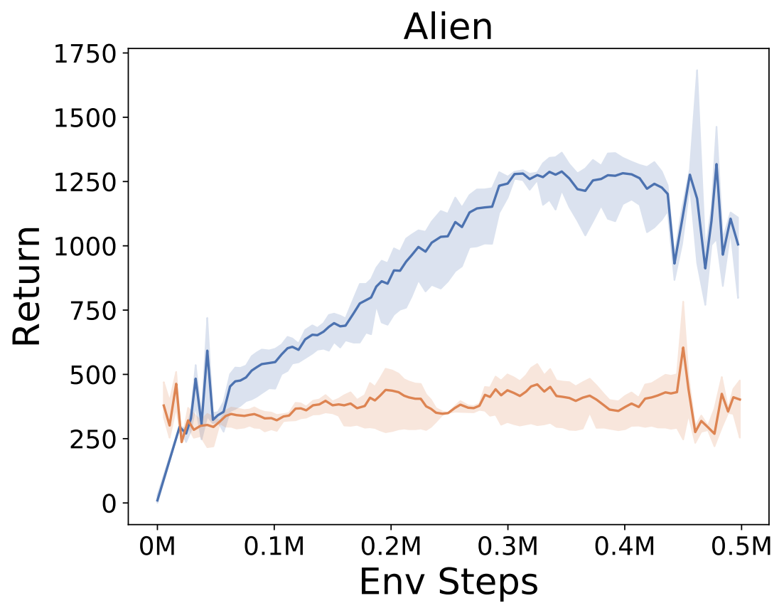
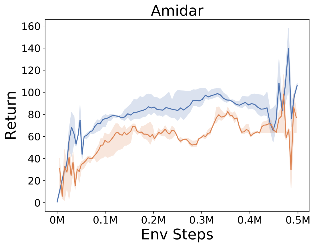
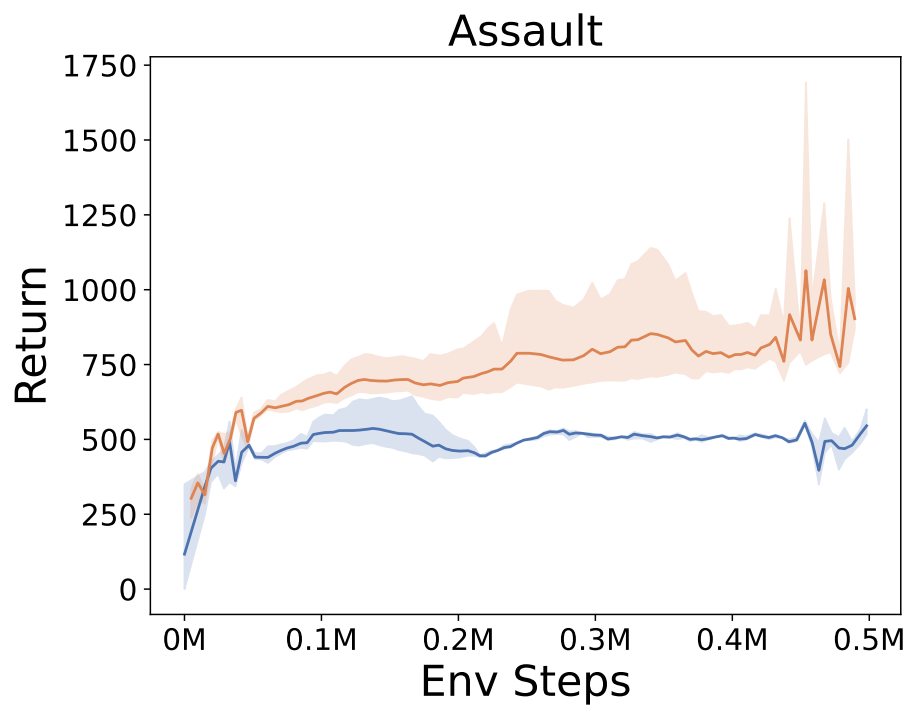
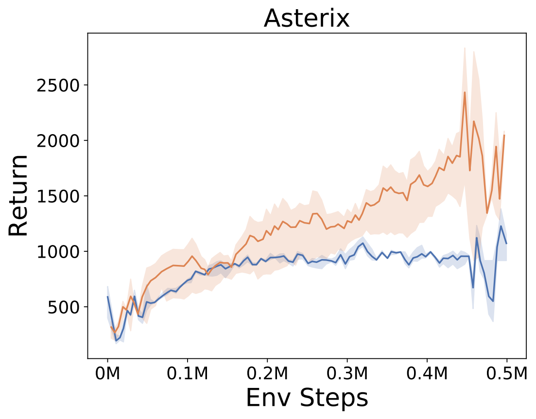
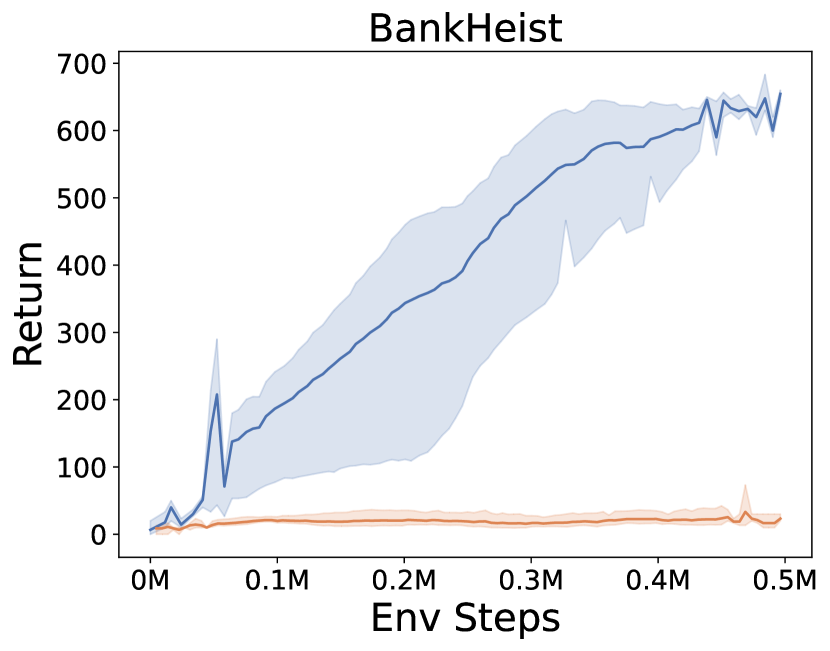
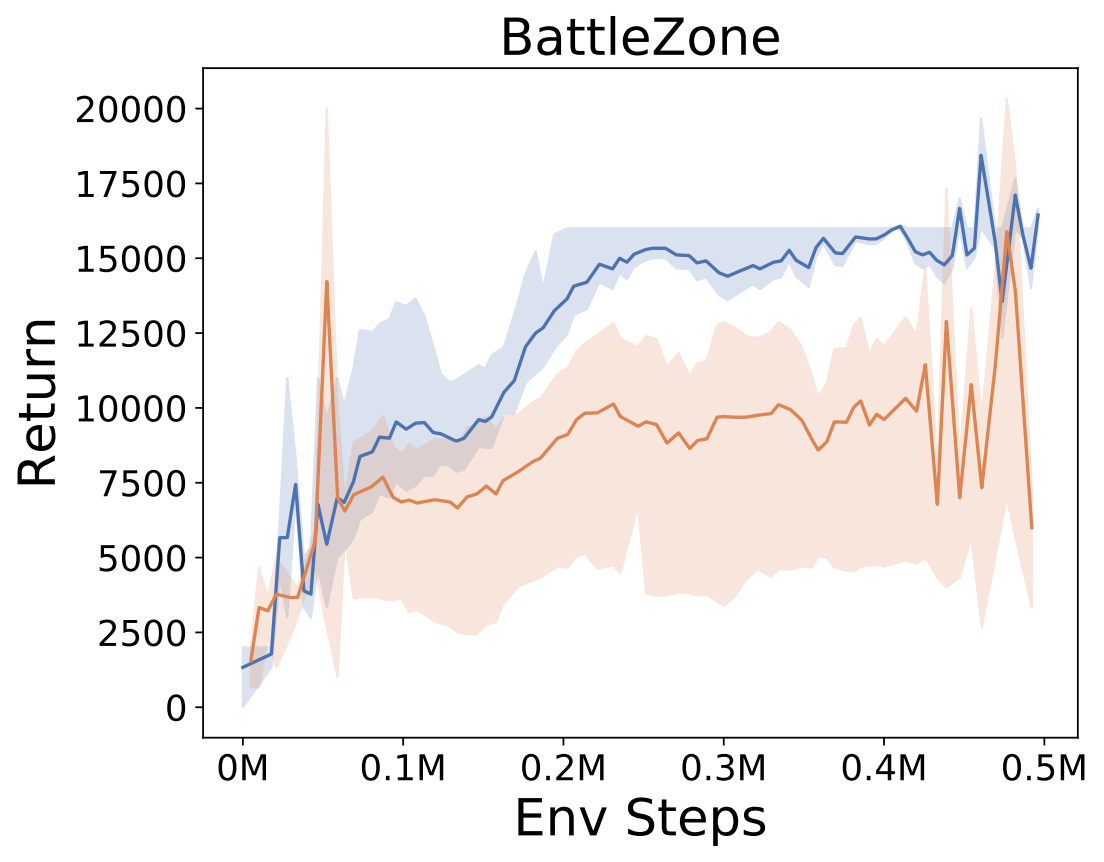
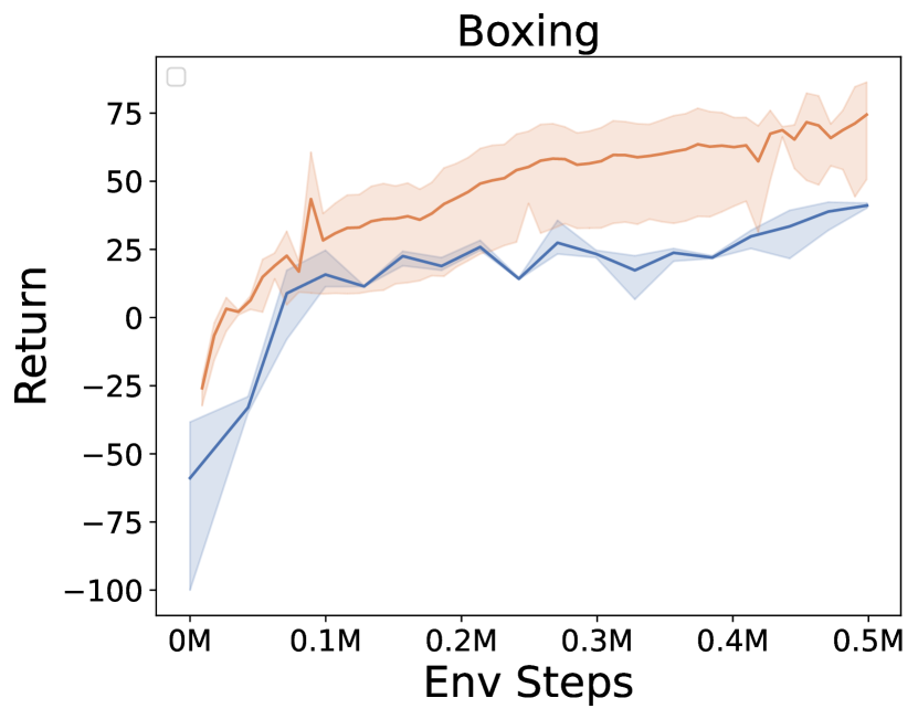
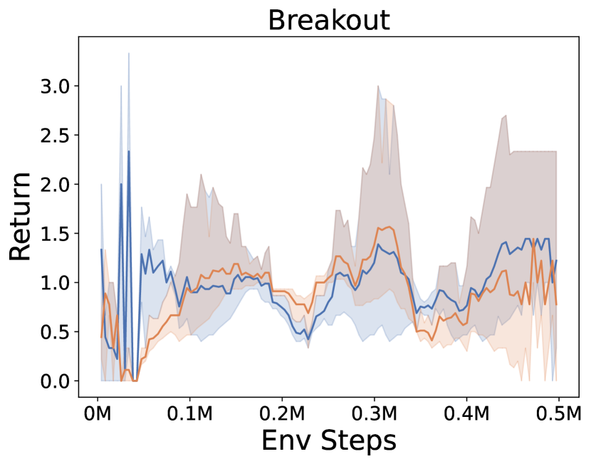
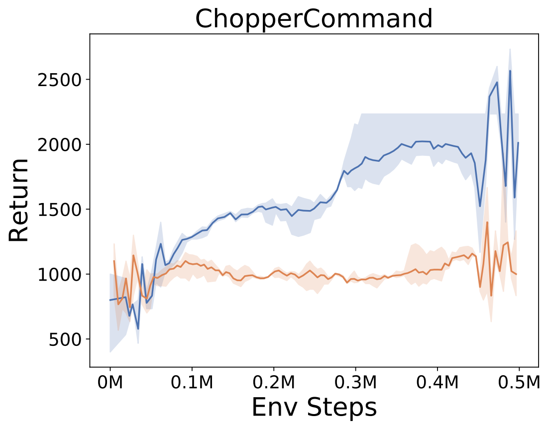
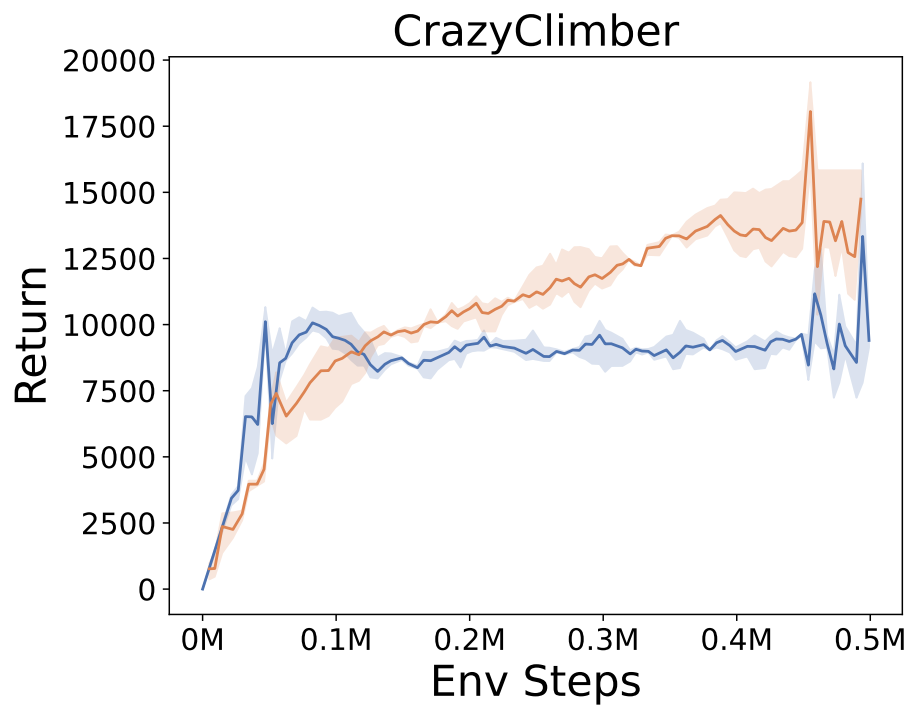
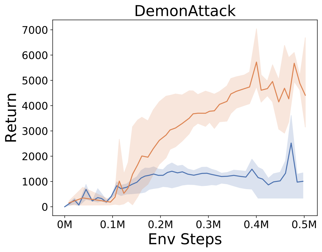
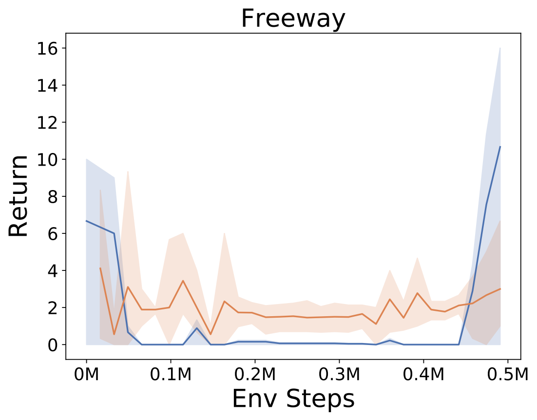
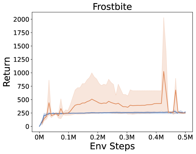
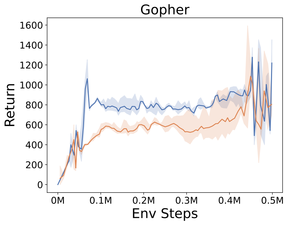
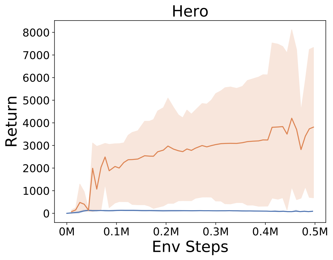
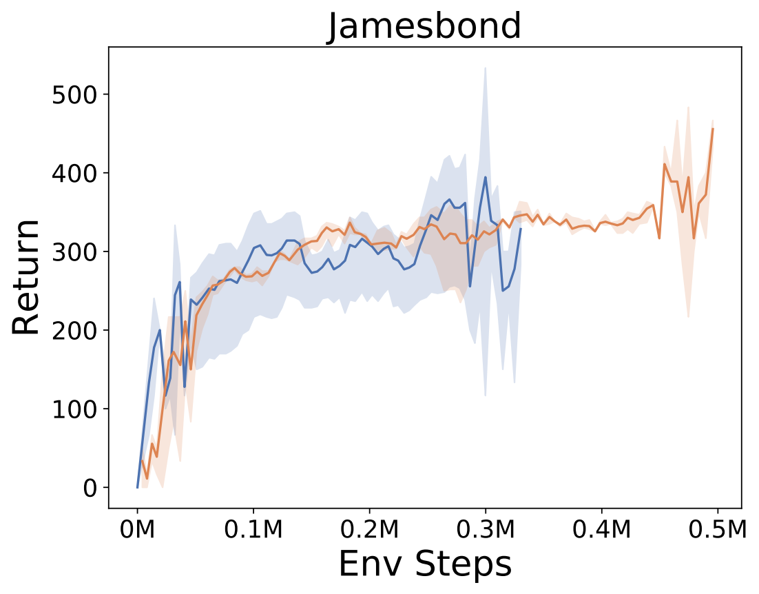
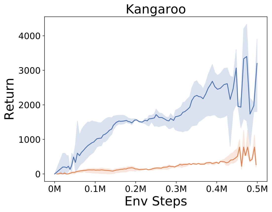
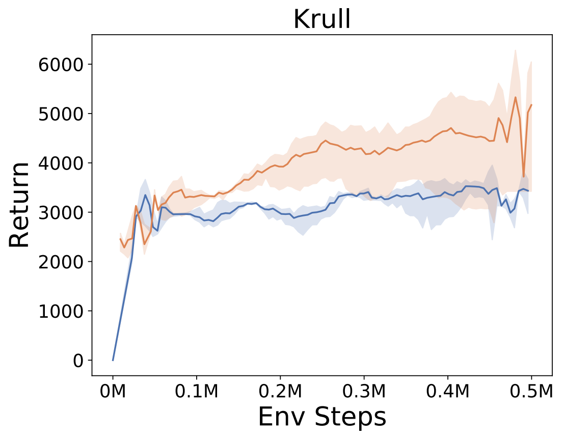
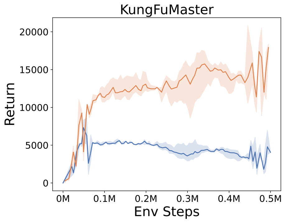
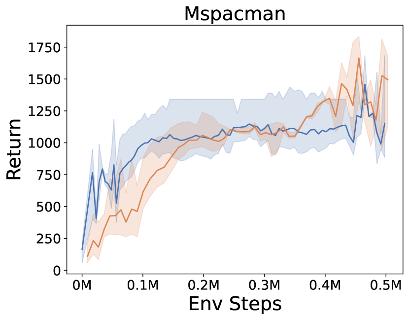
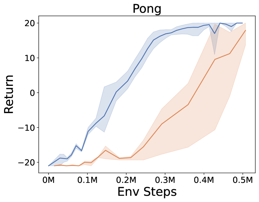
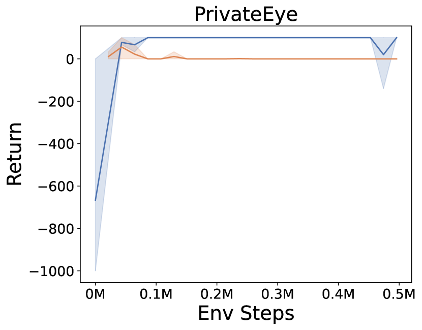
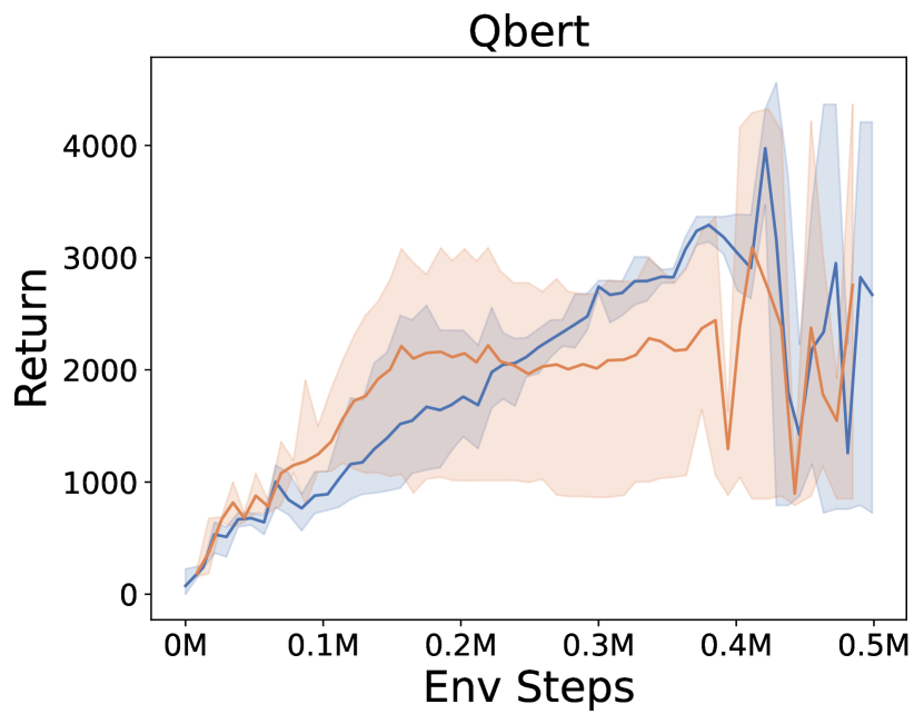
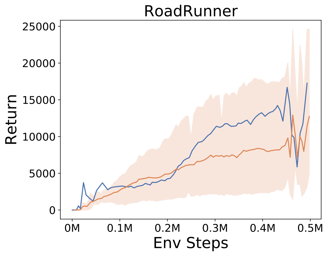
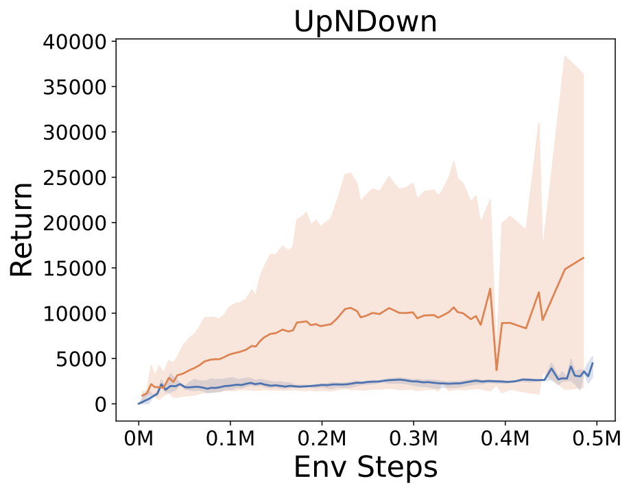
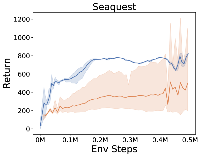
Figure 9: Performance comparison of UniZero with MuZero w/ SSL on the Atari 100k benchmark with reanalyze_ratio=0. Our proposed UniZero is represented in blue, while MuZero w/ SSL is in orange. UniZero outperforms MuZero w/ SSL in 17 out of 26 games, while maintaining comparable performance in most of the remaining games. The solid line represents mean of 3 runs; the shaded areas are 95% confidence intervals.

Appendix D Additional Ablation Study and Analysis

D.1 Ablation Study Details

In Section 4.4, we evaluate the effectiveness and scalability of UniZero’s key designs in Pong. We also present the ablation results for VisualMatch in Figure 10 and target network ablation in Figure 11. Below are the detailed settings for these ablations:

• Model Size Across Different Inference Context Lengths ($H_{\text{infer}}$ = 4/8): Varying the number of layers in the Transformer backbone while keeping the number of heads fixed at 8.

• Training Context Length (H) with Fixed Inference Context Length ($H_{\text{infer}}$ = 4): $H$ is the length of the training sequence.

• Latent Normalization: Comparing SimNorm (default) with Softmax and Sigmoid. These normalization operations are applied to the encoded latent state and the final component of the dynamics network that predicts the next latent state.

• Decode Regularization: Adding a decoder to the latent state from the encoder:

  $$\text{decoder: }\hat{o}_{t}=d_{\theta}(\hat{z}_{t})\color[rgb]{.5,.5,.5}{\vartriangleright\text{Maps latent state to observations for regularization}}$$

  with an auxiliary training objective,

  $$\mathcal{L}_{\text{decode\_reg}}=\|o_{t}-d_{\theta}(z_{t})\|_{1}+\mathcal{L}_{\text{perceptual}}(o_{t},d_{\theta}(z_{t}))\text{ where }z_{t}=h_{\theta}(o_{t})$$

  The first term represents the reconstruction loss, while the second term corresponds to the perceptual loss, similar to the approach described in [2]. In our ablations, the loss coefficient is set to 0.05. It is important to note that in VisualMatch, we solely utilize the first term.

• Target World Model:

  • Soft Target (default): Uses an EMA target model [40] for target latent state and target value.

  • Hard Target: Hard copies the target world model every 100 training iterations.

  • No Target: Does not use the target world model, i.e., the target of the next latent state is produced from the current world model.

From the ablation results, we observe the following findings:

• As shown in Figure 6, for inference context length ($H_{\text{infer}}$ = 4/8), performance at $H_{\text{infer}}$ = 4 consistently outperforms $H_{\text{infer}}$ = 8, regardless of the Transformer’s layer count. This suggests that a shorter context is sufficient for Atari tasks like Pong. Additionally, performance improves with an increased layer count, indicating a moderate model size suffices. However, for VisualMatch, a context length matching the episode length is crucial as the agent needs memory of the target color from phase one. Thus, we set the train context length = 16 + memory_length. As shown in Figure 10, performance increases with model size, indicating that capturing long dependencies requires deeper transformer blocks.

• As shown in Figure 6, with a fixed inference context length ($H_{\text{infer}}$ = 4), performance generally improves with an increased training context length (H), implying that forecasting further into the future aids representation learning, consistent with literature insights.

• SimNorm [7] yields the best results for latent state processing, followed by Softmax, while Sigmoid fails to converge. This underscores the importance of appropriate normalization in the latent space for training stability. SimNorm introduces natural sparsity by maintaining the L1 norm of the latent state at a fixed value, managing gradient magnitudes within a stable range. Gradient explosions often occur without normalization.

• In Pong and VisualMatch, decode regularization has negligible impact on performance, corroborating that more decision-relevant information is required in the latent states, and reconstructing original images is unnecessary.

• As illustrated in Table 11, employing a soft target world model yields the most stable performance. In contrast, the hard target demonstrates some instability, and the absence of a target world model leads to non-convergence in Pong and results in NaN gradients in VisualMatch. Consequently, we do not plot the No target variant in VisualMatch. This behavior parallels the role of target networks in algorithms such as DQN [40].

Figure 10: Ablation study in VisualMatch (MemoryLength=60). Mean of 3 runs, shaded areas are 95% confidence intervals.

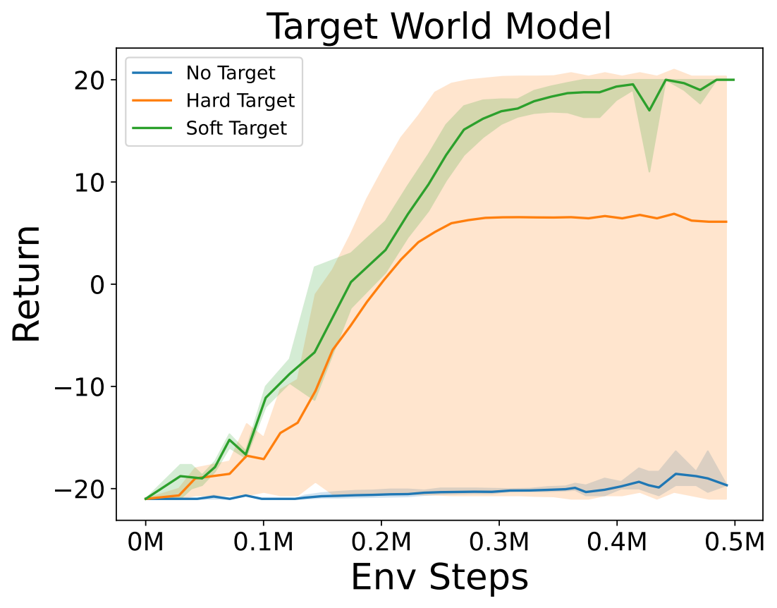
Figure 11: Ablation results of target world model in Pong (Left) and in VisualMatch (MemoryLength=60) (Right). Soft target world model yields the most stable performance. The horizontal axis represents Env Steps, while the vertical axis indicates the Return/Success Rate over 10 episodes. Mean of 3 runs, shaded areas are 95% confidence intervals.

D.2 World Model Analysis

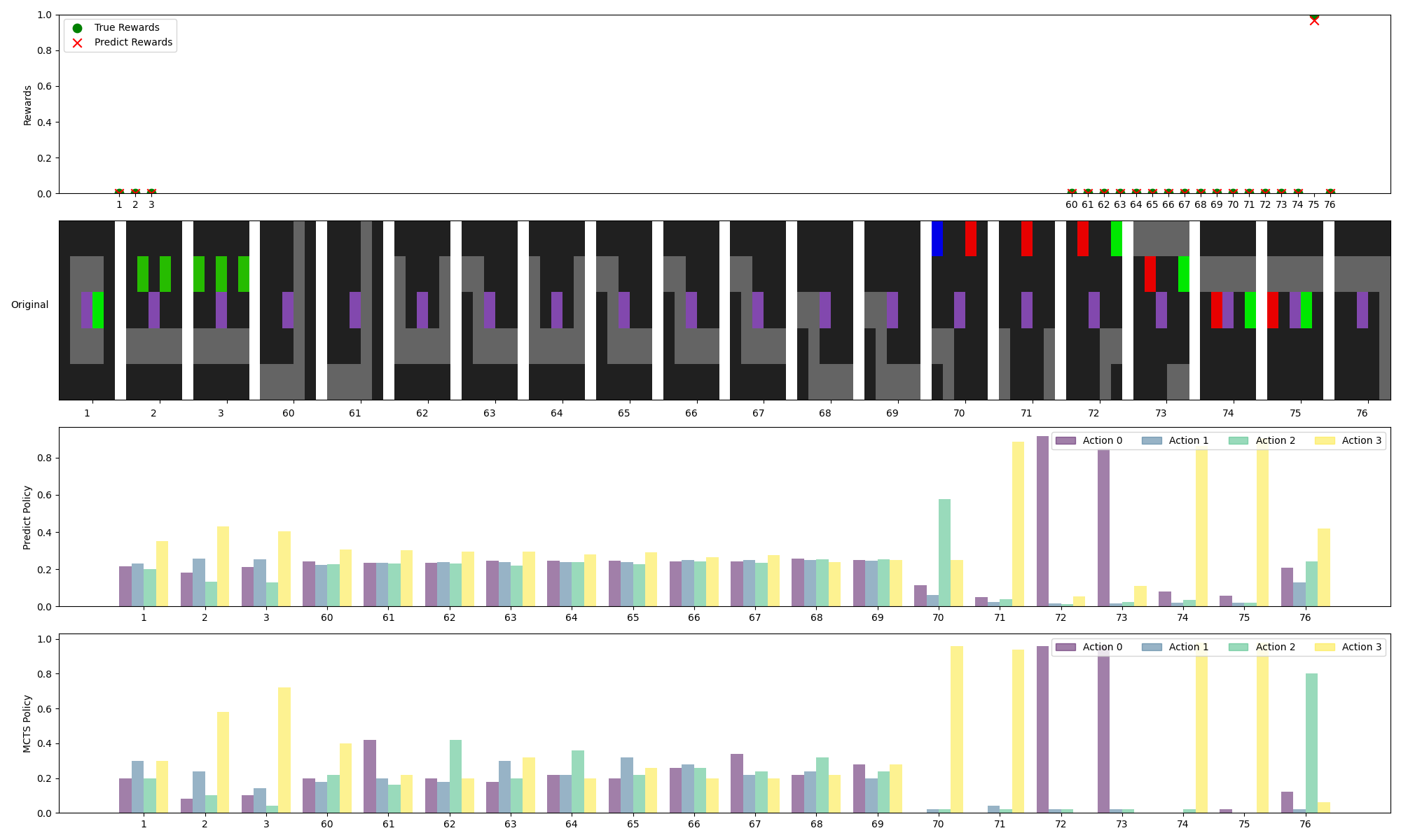
Figure 12: Predictions of the world model in one success episode of VisualMatch (MemoryLength=60). The first row indicates the predicted reward and true reward. The second row displays the original image frame. The third row outlines the predicted prior policy, and the fourth row describes the improved (MCTS) policy induced by MCTS based on the prior policy. For the sake of simplicity, we have only illustrated the first two steps ($t=\{2,3\}$) and the last two steps ($t=\{60,61\}$) of the distraction phase. At timestep 75, action 3, which corresponds to moving to the right, is identified as the optimal action because the target color, green, is located on the agent’s right side. Although the predicted prior policy assigns some probability to actions other than action 3, the MCTS policy refines this distribution, converging more decisively towards action 3.

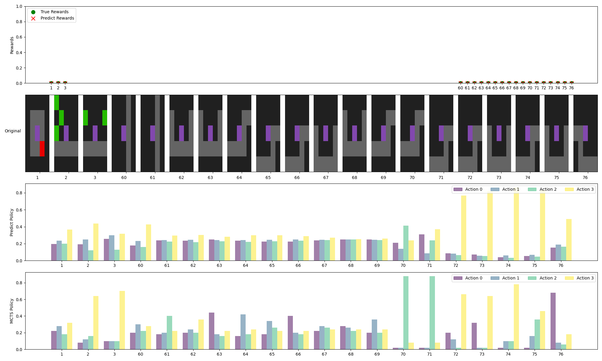
Figure 13: Predictions of the world model in one fail episode of VisualMatch (MemoryLength=60). The first row indicates the predicted reward and true reward. The second row displays the original image frames. The third row outlines the predicted prior policy, and the fourth row describes the improved (MCTS) policy induced by MCTS based on the prior policy.

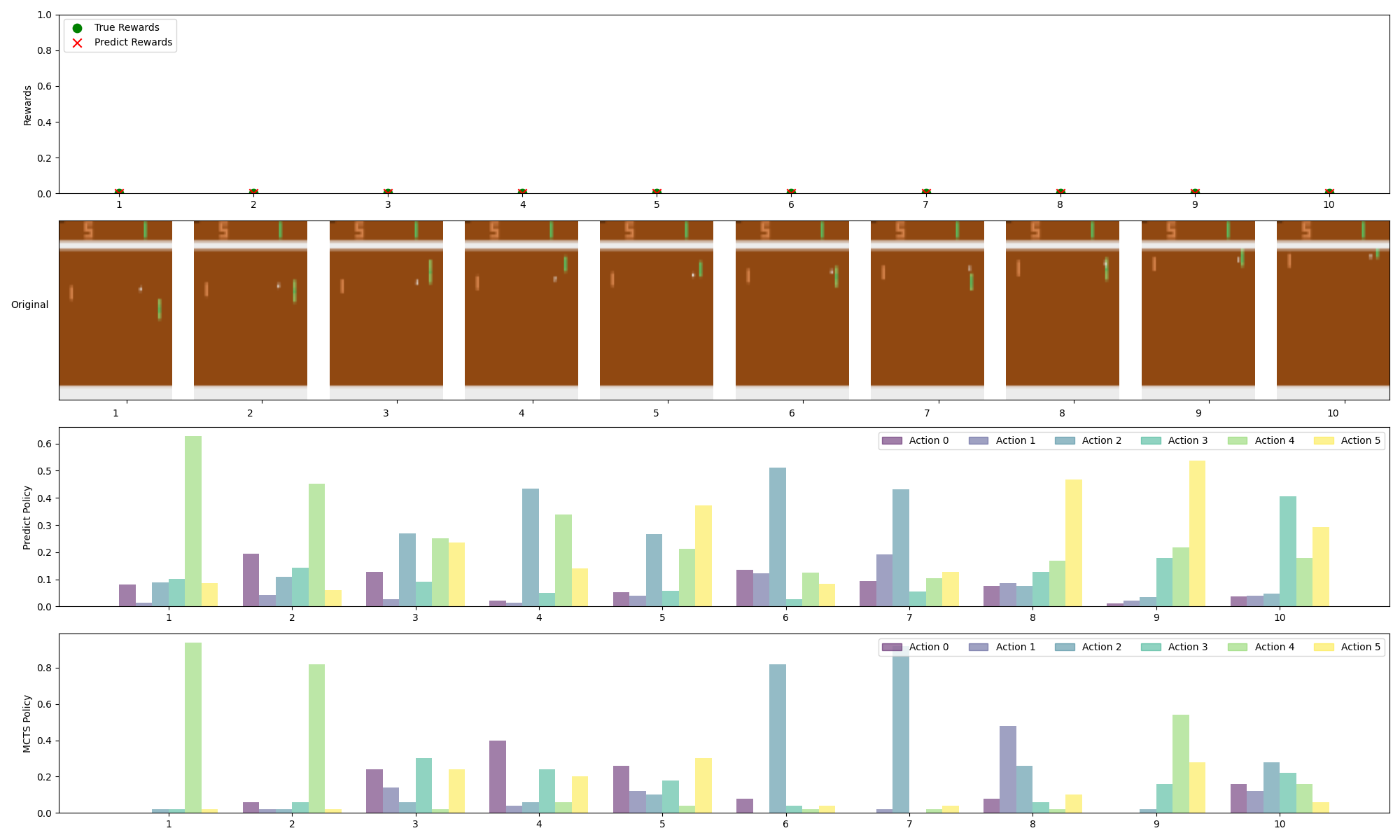
Figure 14: Predictions of the world model in one trajectory of Pong. The first row indicates the predicted reward and true reward. The second row displays the original image frame. The third row outlines the predicted prior policy, and the fourth row describes the improved (MCTS) policy induced by MCTS based on the prior policy.

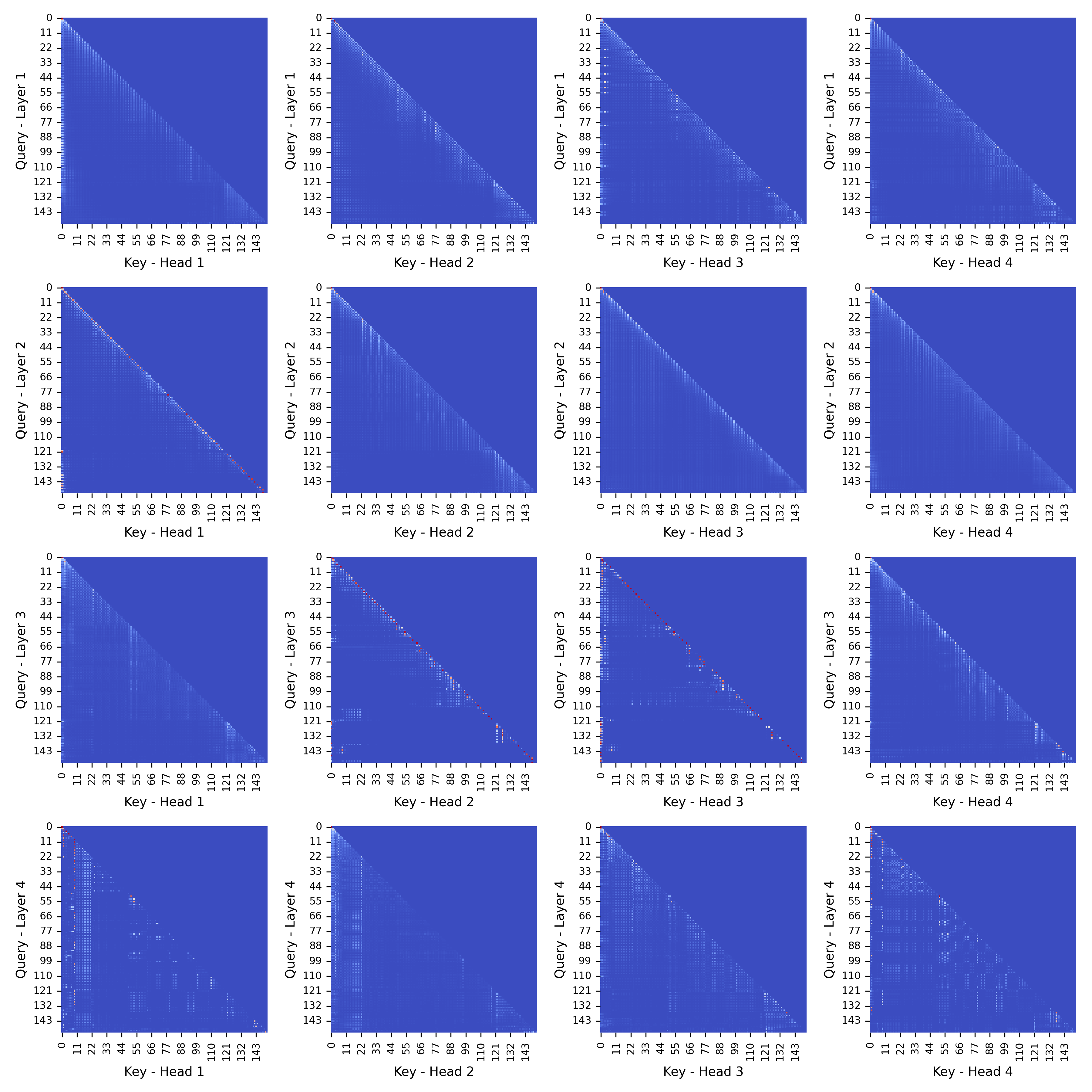
Figure 15: Attention maps in one success episode of VisualMatch (MemoryLength=60) (Note that the train_context_length is $1+60+15=76$, with each time step consisting of two tokens, namely the latent state and the action.). It can be observed that in the initial layers of the Transformer, the attention is primarily focused on the first time step (which contains the target color that needs to be remembered) and the most recent few time steps, mainly for predicting potential dynamic changes. In higher-level layers, sometimes, such as in Layer3-Head2, the attention is mainly concentrated on the current time step, whereas at other times, such as in Layer4-Head4, there is a relatively broad and dispersed attention distribution, possibly indicating the fusion of some learned higher-level features.

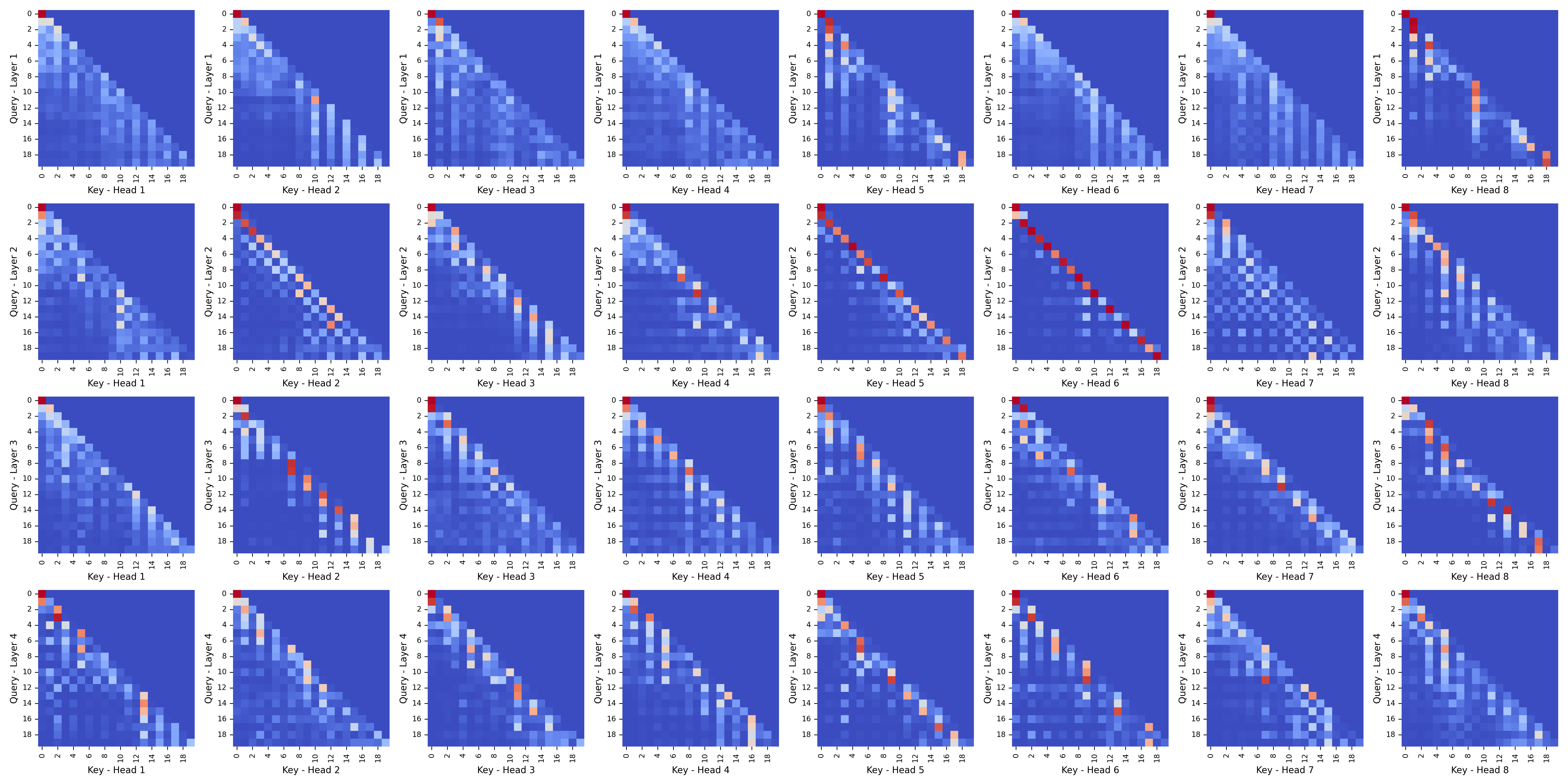
Figure 16: Attention maps in one trajectory (train_context_length is 10, with each time step consisting of two tokens, namely the latent state and the action.) of Pong. It can be observed that across various levels, attention is primarily on data from the most recent frames. This is closely related to the short-term dependency characteristic of Pong. Utilizing information from only the recent frames is sufficient for dynamic prediction and policy-value learning.

VisualMatch.

In Figure 12 and Figure 13, we present the predictions of the learned world model in one success and one fail episode of VisualMatch (MemoryLength=60), respectively. The first row indicates the predicted reward and true reward. The second row displays the original image frame. The third row outlines the predicted prior policy, and the fourth row describes the improved (MCTS) policy induced by MCTS based on the prior policy. For the sake of simplicity, we have only illustrated the first two steps ($t=\{2,3\}$) and the last two steps ($t=\{60,61\}$) of the distraction phase. Please note that at each timestep, the agent performs the action with the highest probability value in the fourth row. As observed, the reward is accurately predicted in both cases, and the MCTS policy has shown further improvement compared to the initial predicted prior policy. For example, in Figure 12, at timestep 75, action 3, which represents moving to the right, is identified as the optimal action because the target color, green, is located on the agent’s right side. While the predicted prior policy still allocates some probability to actions other than action 3, the MCTS policy refines this distribution, converging more towards action 3.

Figure 15 shows the attention maps of the trained world model. It can be observed that in the initial layers of the Transformer, the attention is primarily focused on the first time step (which contains the target color that needs to be remembered) and the most recent few time steps, mainly for predicting potential dynamic changes. In higher-level layers, sometimes, such as in Layer3-Head2, the attention is mainly concentrated on the current time step, whereas at other times, such as in Layer4-Head4, there is a relatively broad and dispersed attention distribution, possibly indicating the fusion of some learned higher-level features.

Pong.

Similarly, in Figure 14, we present the predictions of the world model in one trajectory of Pong. The first row indicates the predicted reward and true reward. The second row displays the original image frame. The third row outlines the predicted prior policy, and the fourth row describes the improved (MCTS) policy induced by MCTS based on the prior policy. Please note that the image in the second row (original image) has already been resized to (64,64) from the raw Atari image, so there may be some visual distortion. At each timestep, the agent performs the action with the highest probability value in the fourth row. Throughout all timesteps, the true reward remains zero due to the absence of score events. Unizero’s world model can accurately predict this, with all predicted rewards consistently remaining zero. At the 8th timestep, the agent controlling the right green paddle successfully bounces the ball back. At the 7th timestep, the agent should perform the upward action 2; otherwise, it might miss the opportunity to catch the ball. The MCTS policy further concentrates the action probability on action 2 compared to the prediction policy, demonstrating the policy improvement process of MCTS.

In Figure 16, we plot the attention maps in one trajectory (train_context_length is 10, with each time step consisting of two tokens, namely the latent state and the action) of Pong. It can be observed that across various levels, attention is primarily on data from the most recent frames. This is closely related to the short-term dependency characteristic of Pong. Utilizing information from only the recent frames is sufficient for dynamic prediction and policy-value learning.

Appendix E Multi-task Learning

UniZero’s decoupled yet streamlined design has enabled it to excel in various single-task problems with differing degrees of dependency (Section 4.1). By leveraging the transformer backbone, we can automatically address these varying levels of dependency. Owing to its unified architecture and training paradigm, UniZero can seamlessly extend to a multi-task learning setup. This section presents preliminary results on four Atari games: Pong, MsPacman, Seaquest, and Boxing, to validate its potential in multi-task learning. Note that unless stated otherwise, the multi-task hyperparameters are consistent with those in Table 6.

Architecture The observation space for each task is uniform, represented as a (3, 64, 64) image. We set full_action_space=True [34], which means that the action space for all tasks is 18. Compared to single-task settings, our primary modification is the establishment of independent decision heads and dynamics heads for each task, following the approach of [66], which introduces only minimal additional parameters. The Transformer backbone network and encoder are shared across tasks. In our initial experiments, we found that using LayerNorm in the encoder was crucial for performance. This is likely due to significant differences in internal state statistics at the early stages of learning for different tasks, leading to performance degradation when using BatchNorm [67].

Training. Each task has its own collector, which sequentially collects trajectories and stores them in their respective replay buffers. During training, we sample task_batch_size=32 samples from different tasks, combine them into a large minibatch, apply the same loss function as in Equation 3 for each task, average the task losses to obtain the final total loss, backpropagate the gradients, and update the entire network.

Results. As illustrated in Figure 17, with minimal adjustments, joint multi-task training on the Atari games Pong, MsPacman, Seaquest, and Boxing achieved comparable sample efficiency across all tasks when compared to single-task learning outcomes. This underscores the potential of UniZero as a scalable latent world model for training generalized agents. It is noteworthy that in our preliminary experiments, we also explored multi-task gradient correction methods such as PCGrad [68] and CAGrad [69], but found their benefits to be minimal. Consequently, these techniques are not included in our experimental results, although a more in-depth analysis is reserved for future work. Future research will focus on effective task balancing, learning dynamics, information reuse in MCTS, the integration of multiple modalities and tasks, and advanced pretraining and fine-tuning techniques, among other areas.

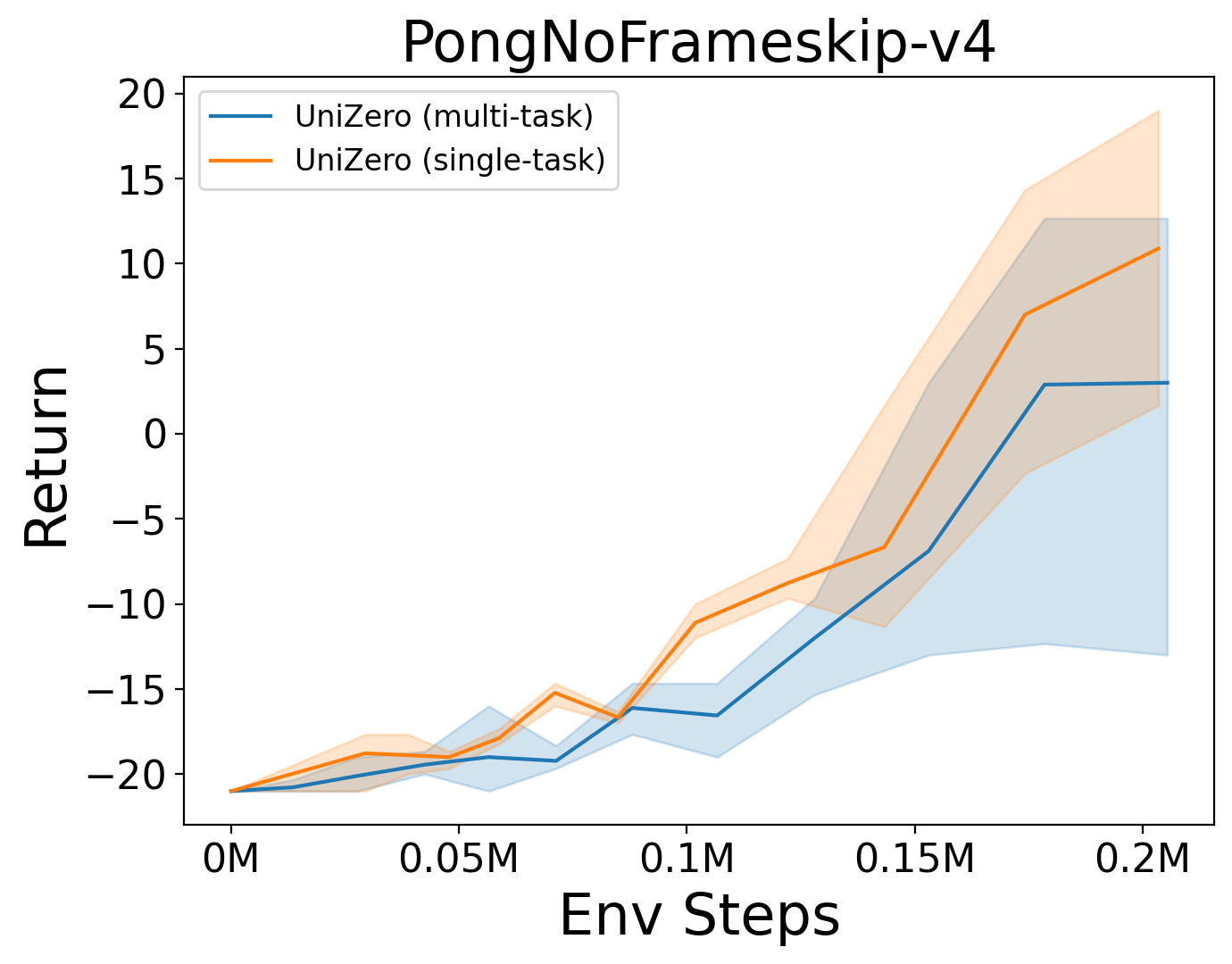
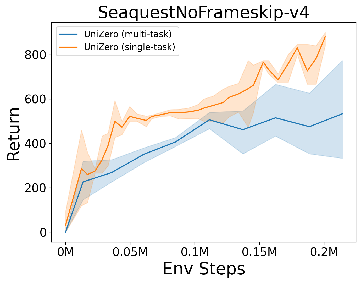
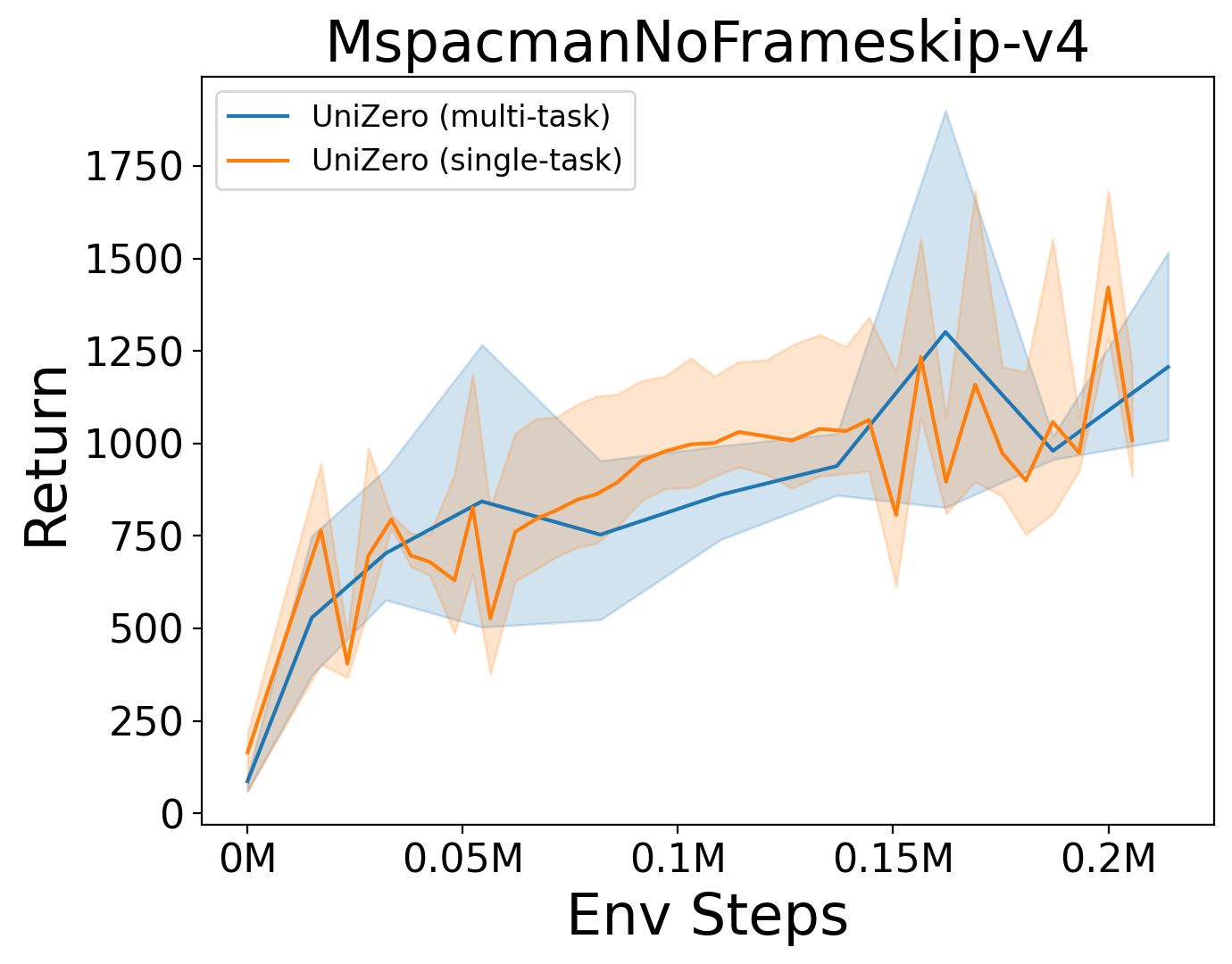
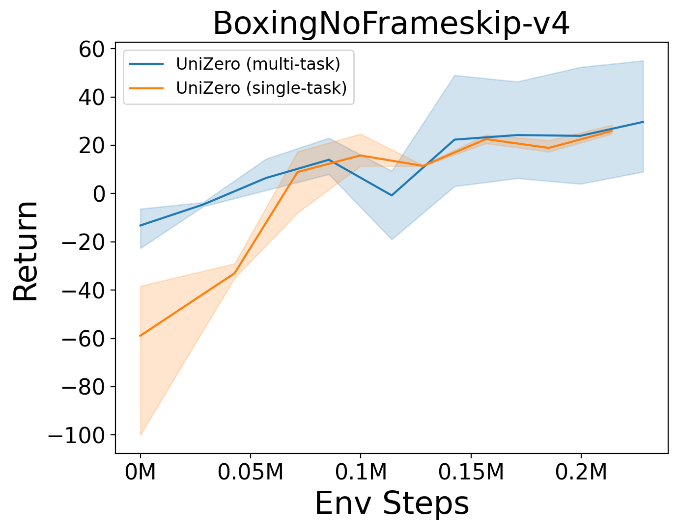
Figure 17: Performance comparison between multi-task and single-task settings on four Atari games: Pong, Ms. Pac-Man, Seaquest, and Boxing. Multi-task training demonstrated comparable sample efficiency across all tasks relative to single-task learning. This highlights the potential of UniZero as a scalable latent world model for training generalized agents. The solid line represents the mean of 3 runs, with the shaded areas indicating the 95% confidence intervals.

Appendix F Comparison with Prior Works

To provide a clear comparison, we present Table 9 outlining the key differences between UniZero and recent approaches [7, 10, 26, 27, 28, 29] in world modeling. The attributes considered include the type of sequence model used, the input information introduced during a single timestep, the method for obtaining latent representations, the approach to policy improvement, and the training pipeline.

• Sequence Model: The architecture employed for modeling sequences.

• Input: The type of information fed into the sequence model at each timestep, where "Latent history" refers to the recurrent/hidden state as described in the respective papers.

• Latent Representation: This refers to the technique employed to extract embeddings from each observation. For instance, an "Encoder" might be a neural network such as a Convolutional Network (ConvNet) for processing images or a Multi-Layer Perceptron (MLP) for handling vector observations. The term "VQ-VAE" [70] denotes the vector-quantized VAE, which is utilized to obtain a discrete code for the observation. Similarly, "Categorical-VAE" [26] represents the discrete VAE, which is used to derive the discrete distribution of the observation.

• Policy Improvement: The method for enhancing the policy, with "PG" standing for Policy Gradient methods [43, 26] and "MPC" standing for Model Predictive Control [55].

• Training Pipeline: The training process involves a "two-stage" approach, where we first train the world model and then use the learned model to train the policy (behavior) through imagination. On the other hand, "model-policy joint training" refers to simultaneously learning the world model and the policy (and value), rather than following a two-stage process. This joint training approach offers several benefits, as discussed in [31, 71, 39].

Table 9: Comparison between UniZero and recent model-based RL approaches. The main difference between UniZero and MuZero is highlighted in bold.

Attributes		Sequence model	Input	Latent representation	Policy Improvement	Training Pipeline
TWM [28]		Transformer-XL [72]	Latent, observation, action, reward	Categorical-VAE	PG of DreamerV2 [6]	two-stage
IRIS [27]		Transformer [19]	Latent, observation, action	VQ-VAE	PG of DreamerV2 [6]	two-stage
DreamerV3 [26]		GRU [73]	Latent, observation, action	Categorical-VAE	PG of DreamerV3	two-stage
STORM [29]		Transformer	Latent, observation, action	Categorical-VAE	PG of DreamerV3	two-stage
TD-MPC2 [7]		MLP	Latent, observation, action	Encoder (with SimNorm)	MPC [55]	two-stage
MuZero [10]		MLP	Latent, action	Encoder	MCTS	Model-policy Joint training
UniZero (ours)		Transformer [74]	Latent, observation, action	Encoder (with SimNorm)	MCTS	Model-policy Joint training

References

- (1) Richard S Sutton and Andrew G Barto. Reinforcement learning: An introduction. MIT press, 2018.
- (2) Tianwei Ni, Michel Ma, Benjamin Eysenbach, and Pierre-Luc Bacon. When do transformers shine in rl? decoupling memory from credit assignment. Advances in Neural Information Processing Systems, 36, 2024.
- (3) Mohammad Reza Samsami, Artem Zholus, Janarthanan Rajendran, and Sarath Chandar. Mastering memory tasks with world models. arXiv preprint arXiv:2403.04253, 2024.
- (4) Marco Pleines, Matthias Pallasch, Frank Zimmer, and Mike Preuss. Memory gym: Partially observable challenges to memory-based agents. In The eleventh international conference on learning representations, 2022.
- (5) Michael Janner, Justin Fu, Marvin Zhang, and Sergey Levine. When to trust your model: Model-based policy optimization. Advances in neural information processing systems, 32, 2019.
- (6) Danijar Hafner, Timothy Lillicrap, Mohammad Norouzi, and Jimmy Ba. Mastering atari with discrete world models. arXiv preprint arXiv:2010.02193, 2020.
- (7) Nicklas Hansen, Hao Su, and Xiaolong Wang. Td-mpc2: Scalable, robust world models for continuous control. arXiv preprint arXiv:2310.16828, 2023.
- (8) Mahmoud Assran, Quentin Duval, Ishan Misra, Piotr Bojanowski, Pascal Vincent, Michael Rabbat, Yann LeCun, and Nicolas Ballas. Self-supervised learning from images with a joint-embedding predictive architecture. In Proceedings of the IEEE/CVF Conference on Computer Vision and Pattern Recognition, pages 15619–15629, 2023.
- (9) Richard S Sutton, Michael Bowling, and Patrick M Pilarski. The alberta plan for ai research. arXiv preprint arXiv:2208.11173, 2022.
- (10) Julian Schrittwieser, Ioannis Antonoglou, Thomas Hubert, Karen Simonyan, Laurent Sifre, Simon Schmitt, Arthur Guez, Edward Lockhart, Demis Hassabis, Thore Graepel, Timothy P. Lillicrap, and David Silver. Mastering atari, go, chess and shogi by planning with a learned model. CoRR, abs/1911.08265, 2019.
- (11) Ivo Danihelka, Arthur Guez, Julian Schrittwieser, and David Silver. Policy improvement by planning with gumbel. In International Conference on Learning Representations, 2022.
- (12) Ioannis Antonoglou, Julian Schrittwieser, Sherjil Ozair, Thomas K Hubert, and David Silver. Planning in stochastic environments with a learned model. In International Conference on Learning Representations, 2021.
- (13) Thomas Hubert, Julian Schrittwieser, Ioannis Antonoglou, Mohammadamin Barekatain, Simon Schmitt, and David Silver. Learning and planning in complex action spaces. In Marina Meila and Tong Zhang, editors, Proceedings of the 38th International Conference on Machine Learning, ICML 2021, 18-24 July 2021, Virtual Event, volume 139 of Proceedings of Machine Learning Research, pages 4476–4486. PMLR, 2021.
- (14) Yazhe Niu, Yuan Pu, Zhenjie Yang, Xueyan Li, Tong Zhou, Jiyuan Ren, Shuai Hu, Hongsheng Li, and Yu Liu. Lightzero: A unified benchmark for monte carlo tree search in general sequential decision scenarios. Advances in Neural Information Processing Systems, 36, 2024.
- (15) Christopher Grimm, André Barreto, Satinder Singh, and David Silver. The value equivalence principle for model-based reinforcement learning, 2020.
- (16) Maciej Świechowski, Konrad Godlewski, Bartosz Sawicki, and Jacek Mańdziuk. Monte carlo tree search: A review of recent modifications and applications. Artificial Intelligence Review, 56(3):2497–2562, 2023.
- (17) David Silver, Thomas Hubert, Julian Schrittwieser, Ioannis Antonoglou, Matthew Lai, Arthur Guez, Marc Lanctot, Laurent Sifre, Dharshan Kumaran, Thore Graepel, et al. Mastering chess and shogi by self-play with a general reinforcement learning algorithm. arXiv preprint arXiv:1712.01815, 2017.
- (18) Matthew Hausknecht and Peter Stone. Deep recurrent q-learning for partially observable mdps, 2017.
- (19) Ashish Vaswani, Noam Shazeer, Niki Parmar, Jakob Uszkoreit, Llion Jones, Aidan N Gomez, Łukasz Kaiser, and Illia Polosukhin. Attention is all you need. Advances in neural information processing systems, 30, 2017.
- (20) Tom Brown, Benjamin Mann, Nick Ryder, Melanie Subbiah, Jared D Kaplan, Prafulla Dhariwal, Arvind Neelakantan, Pranav Shyam, Girish Sastry, Amanda Askell, et al. Language models are few-shot learners. Advances in neural information processing systems, 33:1877–1901, 2020.
- (21) William Peebles and Saining Xie. Scalable diffusion models with transformers. In Proceedings of the IEEE/CVF International Conference on Computer Vision, pages 4195–4205, 2023.
- (22) Zeqiang Lai, Xizhou Zhu, Jifeng Dai, Yu Qiao, and Wenhai Wang. Mini-dalle3: Interactive text to image by prompting large language models, 2023.
- (23) Lili Chen, Kevin Lu, Aravind Rajeswaran, Kimin Lee, Aditya Grover, Michael Laskin, Pieter Abbeel, Aravind Srinivas, and Igor Mordatch. Decision transformer: Reinforcement learning via sequence modeling, 2021.
- (24) Michael Janner, Qiyang Li, and Sergey Levine. Offline reinforcement learning as one big sequence modeling problem, 2021.
- (25) Scott Reed, Konrad Zolna, Emilio Parisotto, Sergio Gomez Colmenarejo, Alexander Novikov, Gabriel Barth-Maron, Mai Gimenez, Yury Sulsky, Jackie Kay, Jost Tobias Springenberg, Tom Eccles, Jake Bruce, Ali Razavi, Ashley Edwards, Nicolas Heess, Yutian Chen, Raia Hadsell, Oriol Vinyals, Mahyar Bordbar, and Nando de Freitas. A generalist agent, 2022.
- (26) Danijar Hafner, Jurgis Pasukonis, Jimmy Ba, and Timothy Lillicrap. Mastering diverse domains through world models. arXiv preprint arXiv:2301.04104, 2023.
- (27) Ajay Mandlekar, Fabio Ramos, Byron Boots, Silvio Savarese, Li Fei-Fei, Animesh Garg, and Dieter Fox. Iris: Implicit reinforcement without interaction at scale for learning control from offline robot manipulation data, 2020.
- (28) Jan Robine, Marc Höftmann, Tobias Uelwer, and Stefan Harmeling. Transformer-based world models are happy with 100k interactions, 2023.
- (29) Weipu Zhang, Gang Wang, Jian Sun, Yetian Yuan, and Gao Huang. Storm: Efficient stochastic transformer based world models for reinforcement learning, 2023.
- (30) Emilio Parisotto, H. Francis Song, Jack W. Rae, Razvan Pascanu, Caglar Gulcehre, Siddhant M. Jayakumar, Max Jaderberg, Raphael Lopez Kaufman, Aidan Clark, Seb Noury, Matthew M. Botvinick, Nicolas Heess, and Raia Hadsell. Stabilizing transformers for reinforcement learning, 2019.
- (31) Benjamin Eysenbach, Alexander Khazatsky, Sergey Levine, and Russ R Salakhutdinov. Mismatched no more: Joint model-policy optimization for model-based rl. Advances in Neural Information Processing Systems, 35:23230–23243, 2022.
- (32) Raj Ghugare, Homanga Bharadhwaj, Benjamin Eysenbach, Sergey Levine, and Ruslan Salakhutdinov. Simplifying model-based rl: learning representations, latent-space models, and policies with one objective. arXiv preprint arXiv:2209.08466, 2022.
- (33) Edward Jay Sondik. The optimal control of partially observable Markov processes. Stanford University, 1971.
- (34) Marc G Bellemare, Yavar Naddaf, Joel Veness, and Michael Bowling. The arcade learning environment: An evaluation platform for general agents. Journal of Artificial Intelligence Research, 47:253–279, 2013.
- (35) Joery A de Vries, Ken S Voskuil, Thomas M Moerland, and Aske Plaat. Visualizing muzero models. arXiv preprint arXiv:2102.12924, 2021.
- (36) Weirui Ye, Shaohuai Liu, Thanard Kurutach, Pieter Abbeel, and Yang Gao. Mastering atari games with limited data. Advances in Neural Information Processing Systems, 34:25476–25488, 2021.
- (37) Adrià Puigdomènech Badia, Pablo Sprechmann, Alex Vitvitskyi, Daniel Guo, Bilal Piot, Steven Kapturowski, Olivier Tieleman, Martín Arjovsky, Alexander Pritzel, Andew Bolt, et al. Never give up: Learning directed exploration strategies. arXiv preprint arXiv:2002.06038, 2020.
- (38) Junyoung Chung, Caglar Gulcehre, KyungHyun Cho, and Yoshua Bengio. Empirical evaluation of gated recurrent neural networks on sequence modeling. arXiv preprint arXiv:1412.3555, 2014.
- (39) Jean-Bastien Grill, Florent Altché, Yunhao Tang, Thomas Hubert, Michal Valko, Ioannis Antonoglou, and Rémi Munos. Monte-carlo tree search as regularized policy optimization, 2020.
- (40) Volodymyr Mnih, Koray Kavukcuoglu, David Silver, Alex Graves, Ioannis Antonoglou, Daan Wierstra, and Martin Riedmiller. Playing atari with deep reinforcement learning. arXiv preprint arXiv:1312.5602, 2013.
- (41) Marc G. Bellemare, Will Dabney, and Rémi Munos. A distributional perspective on reinforcement learning, 2017.
- (42) Danijar Hafner, Timothy Lillicrap, Jimmy Ba, and Mohammad Norouzi. Dream to control: Learning behaviors by latent imagination. arXiv preprint arXiv:1912.01603, 2019.
- (43) John Schulman, Filip Wolski, Prafulla Dhariwal, Alec Radford, and Oleg Klimov. Proximal policy optimization algorithms. CoRR, abs/1707.06347, 2017.
- (44) Suyu Ge, Yunan Zhang, Liyuan Liu, Minjia Zhang, Jiawei Han, and Jianfeng Gao. Model tells you what to discard: Adaptive kv cache compression for llms, 2024.
- (45) Lukasz Kaiser, Mohammad Babaeizadeh, Piotr Milos, Blazej Osinski, Roy H Campbell, Konrad Czechowski, Dumitru Erhan, Chelsea Finn, Piotr Kozakowski, Sergey Levine, Afroz Mohiuddin, Ryan Sepassi, George Tucker, and Henryk Michalewski. Model-based reinforcement learning for atari, 2024.
- (46) Max Schwarzer, Ankesh Anand, Rishab Goel, R Devon Hjelm, Aaron Courville, and Philip Bachman. Data-efficient reinforcement learning with self-predictive representations. arXiv preprint arXiv:2007.05929, 2020.
- (47) Alec Radford, Karthik Narasimhan, Tim Salimans, Ilya Sutskever, et al. Improving language understanding by generative pre-training. Advances in neural information processing systems, 2018.
- (48) Ching Fang and Kimberly L Stachenfeld. Predictive auxiliary objectives in deep rl mimic learning in the brain, 2023.
- (49) David Silver, Aja Huang, Chris J Maddison, Arthur Guez, Laurent Sifre, George Van Den Driessche, Julian Schrittwieser, Ioannis Antonoglou, Veda Panneershelvam, Marc Lanctot, et al. Mastering the game of go with deep neural networks and tree search. nature, 529(7587):484–489, 2016.
- (50) Julian Schrittwieser, Thomas Hubert, Amol Mandhane, Mohammadamin Barekatain, Ioannis Antonoglou, and David Silver. Online and offline reinforcement learning by planning with a learned model. Advances in Neural Information Processing Systems, 34:27580–27591, 2021.
- (51) Chunyu Xuan, Yazhe Niu, Yuan Pu, Shuai Hu, and Jing Yang. Rezero: Boosting mcts-based algorithms by just-in-time and speedy reanalyze. arXiv preprint arXiv:2404.16364, 2024.
- (52) Shibo Hao, Yi Gu, Haodi Ma, Joshua Jiahua Hong, Zhen Wang, Daisy Zhe Wang, and Zhiting Hu. Reasoning with language model is planning with world model. arXiv preprint arXiv:2305.14992, 2023.
- (53) Lucas Lehnert, Sainbayar Sukhbaatar, Paul Mcvay, Michael Rabbat, and Yuandong Tian. Beyond a*: Better planning with transformers via search dynamics bootstrapping. arXiv preprint arXiv:2402.14083, 2024.
- (54) David Ha and Jürgen Schmidhuber. World models. arXiv preprint arXiv:1803.10122, 2018.
- (55) Nicklas Hansen, Xiaolong Wang, and Hao Su. Temporal difference learning for model predictive control. arXiv preprint arXiv:2203.04955, 2022.
- (56) Basil Kouvaritakis and Mark Cannon. Model predictive control. Switzerland: Springer International Publishing, 38:13–56, 2016.
- (57) Tri Dao, Daniel Y. Fu, Stefano Ermon, Atri Rudra, and Christopher Ré. Flashattention: Fast and memory-efficient exact attention with io-awareness, 2022.
- (58) Joshua Ainslie, James Lee-Thorp, Michiel de Jong, Yury Zemlyanskiy, Federico Lebrón, and Sumit Sanghai. Gqa: Training generalized multi-query transformer models from multi-head checkpoints, 2023.
- (59) Max Schwarzer, Johan Samir Obando Ceron, Aaron Courville, Marc G Bellemare, Rishabh Agarwal, and Pablo Samuel Castro. Bigger, better, faster: Human-level atari with human-level efficiency. In International Conference on Machine Learning, pages 30365–30380. PMLR, 2023.
- (60) Christopher D Rosin. Multi-armed bandits with episode context. Annals of Mathematics and Artificial Intelligence, 61(3):203–230, 2011.
- (61) Samuel Lavoie, Christos Tsirigotis, Max Schwarzer, Ankit Vani, Michael Noukhovitch, Kenji Kawaguchi, and Aaron Courville. Simplicial embeddings in self-supervised learning and downstream classification. arXiv preprint arXiv:2204.00616, 2022.
- (62) Dan Hendrycks and Kevin Gimpel. Gaussian error linear units (gelus). arXiv preprint arXiv:1606.08415, 2016.
- (63) Kuang-Huei Lee, Ofir Nachum, Mengjiao Yang, Lisa Lee, Daniel Freeman, Winnie Xu, Sergio Guadarrama, Ian Fischer, Eric Jang, Henryk Michalewski, and Igor Mordatch. Multi-game decision transformers, 2022.
- (64) Jianlin Su, Yu Lu, Shengfeng Pan, Ahmed Murtadha, Bo Wen, and Yunfeng Liu. Roformer: Enhanced transformer with rotary position embedding, 2023.
- (65) Sepp Hochreiter and Jürgen Schmidhuber. Long short-term memory. Neural computation, 9(8):1735–1780, 1997.
- (66) Aviral Kumar, Rishabh Agarwal, Xinyang Geng, George Tucker, and Sergey Levine. Offline q-learning on diverse multi-task data both scales and generalizes. arXiv preprint arXiv:2211.15144, 2022.
- (67) John Bronskill, Jonathan Gordon, James Requeima, Sebastian Nowozin, and Richard Turner. Tasknorm: Rethinking batch normalization for meta-learning. In International Conference on Machine Learning, pages 1153–1164. PMLR, 2020.
- (68) Tianhe Yu, Saurabh Kumar, Abhishek Gupta, Sergey Levine, Karol Hausman, and Chelsea Finn. Gradient surgery for multi-task learning. Advances in Neural Information Processing Systems, 33:5824–5836, 2020.
- (69) Bo Liu, Xingchao Liu, Xiaojie Jin, Peter Stone, and Qiang Liu. Conflict-averse gradient descent for multi-task learning. Advances in Neural Information Processing Systems, 34:18878–18890, 2021.
- (70) Aäron van den Oord, Oriol Vinyals, and Koray Kavukcuoglu. Neural discrete representation learning. In Isabelle Guyon, Ulrike von Luxburg, Samy Bengio, Hanna M. Wallach, Rob Fergus, S. V. N. Vishwanathan, and Roman Garnett, editors, Advances in Neural Information Processing Systems 30: Annual Conference on Neural Information Processing Systems 2017, December 4-9, 2017, Long Beach, CA, USA, pages 6306–6315, 2017.
- (71) Raj Ghugare, Homanga Bharadhwaj, Benjamin Eysenbach, Sergey Levine, and Ruslan Salakhutdinov. Simplifying model-based rl: Learning representations, latent-space models, and policies with one objective. arXiv preprint arXiv:2209.08466, 2022.
- (72) Zihang Dai, Zhilin Yang, Yiming Yang, Jaime Carbonell, Quoc V. Le, and Ruslan Salakhutdinov. Transformer-xl: Attentive language models beyond a fixed-length context, 2019.
- (73) Kyunghyun Cho, Bart van Merrienboer, Caglar Gulcehre, Dzmitry Bahdanau, Fethi Bougares, Holger Schwenk, and Yoshua Bengio. Learning phrase representations using rnn encoder-decoder for statistical machine translation, 2014.
- (74) Nayoung Lee, Kartik Sreenivasan, Jason D. Lee, Kangwook Lee, and Dimitris Papailiopoulos. Teaching arithmetic to small transformers, 2023.