disposition \xpatchcmd\@sec@pppage \setkomafontsection \setkomafontsubsection
The decomposition of stretched Brownian motion into Bass martingales††thanks: This research was funded by the Austrian Science Fund (FWF) [Grant DOIs: 10.55776/P35197 and 10.55776/P35519]. For open access purposes, the authors have applied a CC BY public copyright license to any author accepted manuscript version arising from this submission. We thank Pietro Siorpaes for his valuable feedback and comments during the preparation of this paper.
Abstract
Abstract. In previous work J. Backhoff-Veraguas, M. Beiglböck and the present authors showed that the notions of stretched Brownian motion and Bass martingale between two probability measures on Euclidean space coincide if and only if these two measures satisfy an irreducibility condition.
Now we consider the general case, i.e. a pair of measures which are not necessarily irreducible. We show that there is a paving of Euclidean space into relatively open convex sets such that the stretched Brownian motion decomposes into a (possibly uncountable) family of Bass martingales on these sets. This paving coincides with the irreducible convex paving studied in previous work of H. De March and N. Touzi.
MSC 2020 subject classifications: Primary 60G42, 60G44; secondary 91G20.
Keywords and phrases: optimal transport, Brenier’s theorem, Benamou–Brenier, stretched Brownian motion, Bass martingale
1 Introduction
As in the parallel paper [BBST23] we consider two probability measures and on with finite second moments, denoted by . It is always assumed that dominates in convex order, written , and meaning that holds for all convex functions .
Our object of interest are martingale transports starting from and terminating in , i.e., one-step martingales with initial distribution and terminal distribution . A celebrated result by Strassen [Str65] shows that, under the above assumptions, there always exists a martingale transport from to . We may and shall identify the one-step martingale with the joint law of the random vector . The set of all martingale transports from to is denoted by .
In [BBHK20] and [BBST23] a special martingale transport has been identified: the stretched Brownian motion from to , which uniquely exists for all with . It is defined as the optimizer of the martingale optimal transport problem
| (1.1) |
where is the standard Gaussian measure on . The maximal covariance between two probability measures is defined as
where the set consists of all couplings between and , i.e., probability measures on with marginals and . By [BBHK20, Theorem 2.2], the discrete-time formulation (1.1) is equivalent to the continuous-time martingale optimal transport problem
| (1.2) |
and there exists a unique-in-law optimizer of (1.2). Furthermore, the optimizers of (1.2) and of (1.1) are related via , the values in (1.1) and (1.2) are equal, and can be explicitly constructed from (see Theorem 2.2 in [BBHK20]). Therefore the stretched Brownian motion from to can equivalently be viewed as the law of the one step-martingale , or as the continuous-time martingale with stochastic differential
where is a standard Brownian motion on . In the following we shall freely switch between these two representations of a stretched Brownian motion.
A particularly appealing subclass of stretched Brownian motions consists of Bass martingales.
Definition 1.1 ([BBST23, Definition 1.1]).
Let be a -dimensional Brownian motion with initial distribution , where is a probability measure on . Let be a convex function such that is square-integrable. The martingale
| (1.3) |
is called Bass martingale with Bass measure , initial law , and terminal law .
Martingales of this form where introduced by Bass [Bas83] (in dimension and with a Dirac measure) in order to derive a solution of the Skorokhod embedding problem. Definition 1.1 generalizes this concept to multiple dimensions and non-degenerate starting laws. A Bass martingale is a stretched Brownian motion [BBHK20, Theorem 1.10], but not vice versa.
1.1 The irreducible case
In [BBST23] the following question was answered: under which conditions on and is the stretched Brownian motion from to a Bass martingale? The answer is given by a connectivity assumption on the marginals, called irreducibility.
Definition 1.2 ([BBST23, Definition 1.2]).
For probability measures on we say that the pair is irreducible, if for all measurable sets with and , there exists a martingale transport such that .
The irreducibility assumption is necessary and sufficient for a stretched Brownian motion to be a Bass martingale, as shown in [BBST23, Theorem 1.3]. The analysis of stretched Brownian motion and Bass martingales relies on the following dual formulation of the optimization problem (1.1).
Theorem 1.3 ([BBST23, Theorem 1.4]).
Here, the symbol used as a superscript denotes the convex conjugate of a function, otherwise it is the convolution operator; stands for relative interior, and for the domain of a function.
A technical caveat seems in order: it turns out that the optimizer of (1.4) is not necessarily -integrable. Therefore, in order for the difference of the integrals in (1.4) to be well-defined, attainment of has to be understood in a “relaxed” sense frequently encountered in martingale optimal transport problems; see [BJ16, BNT17, BNS22] and Subsection 1.6 below.
The following simple observation will be of crucial importance for the analysis of the dual problem (1.4): the value of the dual function
| (1.5) |
remains unchanged if the convex function is replaced by , where is an arbitrary affine function. As a consequence, dual optimizers — provided they exist — turn out to be unique, modulo adding affine functions. We thus make the following definition.
Definition 1.4.
Let be a convex function. We write for the equivalence class of nonnegative convex functions of the form , where is an affine function.
We make one more observation which will turn out to be useful: for an optimizing sequence of lower semicontinuous convex functions for the dual problem (1.4) only their values on the closed convex hull of the support of matter. Indeed, defining
we obtain lower semicontinuous convex functions. It follows from the definition (1.5) of the dual function that , so that is an optimizing sequence, too.
The following theorem is an extension of [BBST23, Theorem 1.4]. It characterizes the features of the irreducible case.
Theorem 1.5 (Irreducible case).
Let with . We denote by the closed convex hull of the support of and by its relative interior. Let be an optimizing sequence of convex functions for the dual problem (1.4), satisfying the regularity assumption (1.22).
-
(1)
If the pair is irreducible, then the following assertions hold:
-
(i)
and , for -a.e. , where and the set is defined in (1.10) below.
-
(ii)
There exist representatives and there is a lower semicontinuous convex function , which is unique modulo adding affine functions, such that
(1.6) (1.7) -
(iii)
The function is a dual optimizer for the pair .
-
(iv)
There is a Bass martingale from to as defined in (1.3), with
(1.8)
-
(i)
- (2)
1.2 The main theorem: general case
We turn to the case of a pair which is not necessarily irreducible. We refer to Section 6 for several illustrative examples of this case. As indicated by the title of the present paper, our main result is that the stretched Brownian motion decomposes into a family of Bass martingales. For this purpose, we fix an optimizing sequence of convex functions for the dual problem (1.4), satisfying the regularity assumption (1.22). We also have to ensure that the sequence decreases sufficiently fast to the optimal value , in the sense that
| (1.9) |
We derive from the sequence the Bass paving of into disjoint relatively open convex sets, which are irreducible under any , via
| (1.10) |
In Propositions 2.3 and 2.4 below we will show that (1.10) indeed defines a paving of enjoying the following properties:
-
(i)
,
-
(ii)
for ,
-
(iii)
for .
We can thus decompose the measure into its restrictions to the sets . For example, if there are at most countably many elements , we have
In general, the Bass paving consists of uncountably many elements, see Example 6.2 below. Following [DMT19], we can still decompose the probability measure as
| (1.11) |
where is a Borel probability measure on the Polish space of closed convex subsets of , equipped with the Wijsman topology [Bee91]. Here, the collection of closed convex sets is isomorphically identified with the collection of their relative interiors. For each , we denote by the closure of .
Using the stretched Brownian motion , we define
| (1.12) |
We thus obtain a decomposition of the probability measure via
| (1.13) |
We now can formulate our main result.
Theorem 1.6 (General case).
Let with . Let be a sequence of convex functions satisfying the regularity assumption (1.22) and the “fast convergence condition” (1.9). Then there is a Bass paving , a Borel probability measure on , and -a.s. unique families of probability measures and in , as in (1.11) and (1.12) above, such that the following assertions hold for -a.e. :
-
(i)
, , and .
-
(ii)
There exist representatives and there is a lower semicontinuous convex function , which is unique modulo adding affine functions, such that
(1.14) (1.15) -
(iii)
The function is a dual optimizer for the pair .
-
(iv)
There is a Bass martingale from to as defined in (1.3), with
(1.16) The Bass martingale coincides with the stretched Brownian motion restricted to .
-
(v)
The pair is irreducible.
A remarkable message of Theorem 1.6 is that an arbitrary sequence of convex functions of class (1.22), such that converges sufficiently fast (see (1.9)) to the optimal value , already contains the full information about the structure (1.16) of the family of Bass martingales from to . Note that in (1.14) and (1.15) we did not have to pass to subsequences or convex combinations of the sequence in order to obtain pointwise convergence.
We can also show that the Bass paving satisfies the maximality condition (1.17) below, as defined in [DMT19, Theorem 2.1]. In particular, Corollary 1.7 states that the martingale transport is an element of the class of maximal transports , considered by H. De March and N. Touzi in [DMT19] (compare also [OS17]).
Corollary 1.7.
Let be an arbitrary martingale transport. For -a.e. , we have that
| (1.17) |
1.3 A guided tour through the proof of Theorem 1.6
Let be a sequence of convex functions satisfying the regularity assumption (1.22) and the “fast convergence condition” (1.9). We define the Bass paving as in (1.10) above. We will show in Propositions 2.3 and 2.4 below that this indeed defines a paving of into relatively open convex sets.
Next, we show that the function given by
| (1.18) |
where is equipped with the Wijsman topology, is Borel measurable. We then define to be the pushforward measure of under the function (1.18), which gives a Borel probability measure on . Applying the disintegration theorem yields the -a.s. unique family of probability measures in , as in (1.11) above. In the following, all statements have to be understood for -a.e. , or for -a.e. .
For fixed , we use and the stretched Brownian motion to define as in (1.12) above. Restricting the stretched Brownian motion to yields the martingale transport
| (1.19) |
from to , so that
| (1.20) |
It is not hard to verify (see Lemma 3.1 below) that actually is the stretched Brownian motion from to . The crucial result is that it is, in fact, a Bass martingale from to . Let us sketch the argument how to find the dual optimizers corresponding to this family of Bass martingales.
For , we consider representatives such that the sequence is bounded. For example, by Hahn–Banach, we can choose so that . By definition (1.10), for , the representatives are pointwise bounded on . We can even obtain pointwise convergence on to a limiting function by choosing (possibly different) representatives . A possible way to find these representatives is to choose a maximal set of affinely independent points in and prescribe arbitrary real values at these points. Then there are affine functions such that attains these values on , i.e.,
| (1.21) |
The functions are uniquely determined by (1.21) on the affine span of . By properly choosing , we can also make sure that , so that . Relying on [BBST23, Proposition 7.20], we come to a crucial point: it turns out that this sequence of representatives indeed converges pointwise to some as in (1.14) and (1.15).
1.4 Literature
Pavings associated to martingale transports into relatively open convex sets, which are invariant under — such as the above Bass paving — have been studied, notably in [OS17, BJ16, DMT19, GKL19, Cio23a, Cio23b].
In [GKL19], N. Ghoussoub, Y.-H. Kim and T. Lim focused on such decompositions, for a fixed martingale transport . They obtained descriptions for the minimizers and maximizers for the cost function , when marginals are supported on , as well as for marginals on higher-dimensional state spaces that are in subharmonic order. Given a specific martingale , Ghoussoub–Kim–Lim also defined a finest paving of the source space into cells that are invariant under the martingale .
While in dimension the decomposition constructed in [GKL19] does not depend on the choice of (see the paper [BJ16] by M. Beiglböck and N. Juillet), it was noted by H. De March and N. Touzi in [DMT19] that in dimension this decomposition does depend on this choice. In [DMT19] and, independently, in the work [OS17] by J. Obłój and P. Siorpaes, the finest such decomposition which works for all was analyzed. In [DMT19] it was shown that such a universal decomposition exists uniquely (in an almost sure sense). In addition, a martingale transport has been constructed in [DMT19], which generates this universal decomposition into irreducible sets. While there is no uniqueness in the construction of such De March–Touzi martingale transports in [DMT19], Theorem 1.6 above shows, among other features, that the (unique) stretched Brownian motion is such a De March–Touzi martingale transport. In particular, the irreducible pavings into relatively open convex sets induced by and coincide (in an almost sure sense made precise below).
1.5 Definitions and notation
-
•
We write for the probability measures on and for the subset of probability measures satisfying , for .
-
•
For , we denote by the set of all couplings between and , i.e. probability measures on with first marginal and second marginal .
-
•
We say that is dominated by in convex order and write , if for all convex functions we have .
-
•
For with we define the collection of martingale transports as those couplings with barycenter , for -a.e. . Here, the family of probability measures is obtained by disintegrating the coupling with respect to its first marginal , i.e., .
-
•
The -dimensional standard Gaussian distribution is denoted by .
-
•
We denote by the set of continuous functions with quadratic growth, meaning that there are constants with
We also introduce the set
(1.22) -
•
For two measures and on we write for their convolution. If is a function, the convolution of and is defined as
provided . In particular, .
-
•
For a function , its convex conjugate is given by
and we write
for the domain of .
-
•
We write and for the relative interior and the closure of a set , respectively.
-
•
The support and the closed convex hull of the support of a measure are denoted by and , respectively.
-
•
The Polish space of closed convex subsets of is equipped with the Wijsman topology [Bee91] and is isomorphically identified with .
1.6 Relaxed formulation of the dual function
Let us return to the technical caveat we made after the statement of Theorem 1.3. For , we recall the definition (1.5) of the dual function , which we rewrite as
| (1.23) |
with being an arbitrary fixed element of . As shown in [BBST23, Proposition 4.2], the dual function written in the “relaxed” form (1.23) is well-defined and takes values in the interval , for a general convex function which is -a.s. finite. Furthermore, by [BBST23, Lemma 3.5] and [BBST23, Proposition 4.1], the value of the dual problem (1.4) is equal to
| (1.24) |
Thus, whenever convenient, by (1.24) we are free to choose optimizing sequences for the dual problem (1.4) of class , as defined in (1.22) above.
Definition 1.8.
2 Equivalence classes of convex functions on
In this section we will analyze some phenomena arising for the equivalence classes of convex functions modulo adding affine functions, as in Definition 1.4.
Definition 2.1.
Let be a convex function. For and , we denote by the equivalence class of convex functions of the form
| (2.1) |
where runs through all affine functions on such that
| (2.2) |
Definition 2.2.
Let be a sequence of real-valued convex functions on . For , we define the sets
| (2.3) | ||||
| (2.4) | ||||
| (2.5) |
Here, the superscripts “b” and “B” stand for “bounded” and “Bass”, respectively. The operator denotes the relative interior of a set. We will prove in Proposition 2.4 below that definition (1.10) of coincides with Definition 2.2, thus justifying this abuse of notation.
Proposition 2.3.
Let be a sequence of real-valued convex functions on . The collection , as introduced in Definition 2.2 above, has the following properties:
-
(i)
,
-
(ii)
for we have ,
-
(iii)
for we have .
In conclusion, the collection is a paving of into relatively open convex sets.
Proof of Proposition 2.3.
(i): Let . We first note that both and are convex sets and by definition the latter set is relatively open. Moreover, it is clear that . To show that is in the relative interior of , we suppose that , i.e., that is a relative boundary point of . By [Roc70, Corollary 11.6.2] there exists a functional and some such that
| (2.6) |
For notational convenience and without loss of generality we assume that . We will show that
| (2.7) |
so that , which will yield the desired contradiction.
We draw a straight line through and , i.e., we consider the function
| (2.8) |
For , let us consider the point on this line. By (2.6) the point cannot be an element of . Thus, for we can find and a function such that
| (2.9) |
By elementary geometry we observe that the convex function in (2.9) has the following property: the affine function on the real line given by
| (2.10) |
is less than or equal to the restriction of to the line (2.8), i.e., the function
By Hahn–Banach we can extend the function to an affine function defined on such that for all . Note that we have . Therefore the function
is a representative of . At the same time we have and thus
This contradicts the assumption and finishes the proof of (i).
(ii): Let . We first show the following claim: For every compact subset there is and such that for each and we have
| (2.11) |
For the proof of the claim, we define the set
By Definition 2.2, we have
We denote by the affine span of and by the relative interior of in . Then for every compact subset we have
By compactness there is some and such that
which readily implies (2.11).
Let and choose such that
Take and such that (2.11) is satisfied for . Now we make the following claim: There exists a constant such that, for every and every choice of representatives and , the affine functions
satisfy the Lipschitz estimate
| (2.12) |
Negating the claim, we suppose that, for every , there is a point and such that
We then obtain
Using the estimates , , and , we conclude that
which is a contradiction to , thus finishing the proof of (2.12).
Finally, it follows from (2.12) that
| (2.13) |
To obtain the full assertion (ii) from (2.13), we still have to show that , and therefore also , is contained in the affine space . If this were not the case, the affine space spanned by would strictly contain . Reversing the roles of and , and applying (2.12) to rather than , we arrive at the desired contradiction, which completes the proof of (ii).
We next show a variant of Proposition 2.3, where we do not have to refer to as in Definitions 2.1 and 2.2 above.
Proposition 2.4.
Let be a sequence of -valued convex functions on . Fix representatives , , and as defined in Definition 2.2. The sequence is bounded for some if and only if it is bounded for all . In this case, is uniformly bounded on compact subsets of .
Proof.
Let be a null sequence and take . By definition (2.3), (2.4) of , we have that is bounded, for all . For arbitrary representatives we have that is an affine function on . As , we have that is bounded from below, for every . If we also have that is bounded, for some , we obtain that is bounded. This implies that is bounded, for all in the affine span of . In particular, is bounded, for all . By convexity, is uniformly bounded on compact subsets of .
As regards the final assertion, the set defined in (1.10) obviously is contained in the set defined in (2.3), (2.4). For the reverse inclusion, suppose there is and a sequence such that is unbounded, while, for every choice of representatives with , the sequence is bounded. This is a contradiction to the first part of Proposition 2.4, finishing the proof of the final assertion. ∎
So far, the sequence of real-valued convex functions on had nothing to do with the pair . We now impose the additional assumption that is an optimizing sequence of convex functions for the dual problem (1.4). In this way, we can relate the support of to .
Proposition 2.5.
Let with . Let be an optimizing sequence of convex functions for the dual problem (1.4), with induced Bass paving . Suppose that there is such that, for , we have . Then for we have
| (2.14) |
Proof.
Applying [BBST23, Lemma 7.9] gives
| (2.15) |
Arguing by contradiction, we assume that (2.14) is not true. Then we can find an open half space with such that . By Proposition 2.4, we can choose representatives such that the sequence is pointwise bounded on . We denote by the function which coincides with on , and assumes the value outside of . As observed after Definition 1.4, the sequence still is an optimizing sequence of lower semicontinuous convex functions in . It also (trivially) satisfies
| (2.16) |
Since , we can find a compact subset such that
| (2.17) |
As a consequence of (2.17), the set has positive -measure.
Now observe that (2.15) also holds when we replace by . Furthermore, as
for -a.e. , we conclude that
As is uniformly bounded on compact subsets of , we have
Consequently,
Using the fact that , we have
| (2.18) |
Next we define a probability measure on by
with normalizing constant
Note that since . In terms of , we can express the right-hand side of (2.18) as
Applying Jensen’s inequality yields
| (2.19) |
where
denotes the barycenter of the probability measure . Observing that and using (2.16), the right-hand side of (2.19) is equal to . This is a contradiction to the finiteness of and shows the inclusion (2.14). ∎
Proposition 2.6.
Let with . Let be an optimizing sequence of convex functions for the dual problem (1.4). Suppose that there is such that for we have . Then there exist representatives and a lower semicontinuous convex function such that
| (2.20) | |||||
| (2.21) |
Furthermore,
| (2.22) |
and the function is a dual optimizer for the pair .
Proof.
Note that by assumption and by Proposition 2.5. Furthermore, by Proposition 2.4, we can choose representatives such that the sequence is pointwise bounded on , i.e.
By [BBST23, Proposition 7.20], we conclude that there are representatives such that (2.20) and (2.21) are satisfied; moreover, we have the identity (2.22), and is a dual optimizer. ∎
In order to apply the disintegration theorem, we will need the following measurability property of the Bass paving .
Proposition 2.7.
Let be a sequence of convex functions. The map given by
| (2.23) |
where is equipped with the Wijsman topology, is Borel measurable.
Proof.
As noted in [DMT19], it suffices to show that the set
is Borel measurable, for every open set . To see this, we fix an open set and note that
Consequently,
Hence is Borel measurable if we can show that the last intersection can be replaced by a countable intersection. In order to do so, we fix a basis of as well as representatives , and define the equivalence class to consist of all functions such that the affine function has rational coefficients when expressed in the basis . We then have to show that
Clearly , so that it remains to show the inclusion . Fix and such that and , i.e., . Choose such that we still have
Note that is bounded from below by and that the function is in , so that for outside a bounded set. Hence we can find a representative such that
Therefore . This shows the claim and we conclude that the set is Borel measurable. ∎
Having established the Borel measurability of the map , we can disintegrate the probability measure with respect to this mapping.
Lemma 2.8.
Let be a sequence of convex functions. Define to be the pushforward measure of under the map of (2.23), which induces a probability measure on (recall that we identify with ). There exists a -a.s. unique family of probability measures such that , for -a.e. , and
| (2.24) |
We refer to Examples 6.1 and 6.2 below for a concrete visualization of Lemma 2.8. For example, the measure in Example 6.1, considered as a probability measure on , gives probabilities to and , as well as probability to the singleton . The Bass paving consists of the relatively open sets , , , where has measure zero with respect to and may therefore be neglected. The probability measures and are the normalized restrictions of to and , respectively.
3 The decomposition of the primal problem
The disintegration result of Lemma 2.8 allows us to decompose the primal problem (1.1) from to into a family of local primal problems, defined on -a.e. set . To this end, we define (as in (1.12) above) the -a.s. unique family of probability measures by
| (3.1) |
where is the optimizer of the primal problem (1.1). As noted in (1.13), the family then is a decomposition of , i.e.
| (3.2) |
By construction we have that , for -a.e. . We obtain the following decomposition of the primal problem (1.1).
Lemma 3.1 (Decomposition of the primal problem).
For -a.e. , the optimizer of the local primal problem
from to equals
| (3.3) |
In particular,
| (3.4) | ||||
| (3.5) | ||||
| (3.6) |
In other words, the martingale transport of (3.3) above is the stretched Brownian motion from to .
Proof of Lemma 3.1.
We note that (3.4) and (3.5) follow from the definition of stretched Brownian motion and (2.24), respectively. Therefore we only have to show the equality (3.6). By contradiction, suppose there is a measurable set with and a -measurable function
such that
Now for define
and
But then for the primal problem from to we have
which is a contradiction to the optimality of . ∎
4 The decomposition of the dual problem
Let be an optimizing sequence of convex functions. In the sequel, we have to assume that the values converge sufficiently fast to the optimal value . To this end, we define the suboptimality functional
| (4.1) |
measuring the difference of from the optimal value . In Lemma 4.1 below we will see that the “fast convergence condition”
| (4.2) |
on , which we have already introduced in (1.9) above, implies that the sequence is not only optimal for the pair , but also for -a.e. pair .
For a fixed set we consider, by analogy with (1.24), the local dual problem from to
where the local dual function now is given by
Similarly as in (4.1), we define the local suboptimality functional
Lemma 4.1 (Decomposition of the dual problem).
-
(i)
For a convex function we have
(4.3) -
(ii)
Let be a sequence of convex functions satisfying (4.2). Then, for -a.e. , we have that is an optimizing sequence for the local dual problem from to , i.e.
(4.4)
Proposition 4.2.
Let be a sequence of convex functions satisfying (4.2). Then the following assertions hold for -a.e. :
- (i)
-
(ii)
There exist representatives and there is a lower semicontinuous convex function such that
(4.6) (4.7) -
(iii)
The function is a dual optimizer for the pair .
5 The proofs of Theorems 1.5, 1.6, and Corollary 1.7
Combining the results of Sections 2 – 4 allows us to finally provide the proof of our main result, Theorem 1.6.
Proof of Theorem 1.6:.
As always, let with . Throughout the proof we fix a sequence of convex functions satisfying (4.2) and consider the Bass paving of Definition 2.2, induced by this sequence. In the following, all statements about a set have to be understood in a -a.s. sense. Once again we emphasize that the “fast convergence condition” (4.2) ensures that is an optimizing sequence for the local dual problems from to . Note that the assertions (i) – (iii) of Theorem 1.6 precisely correspond to the assertions (i) – (iii) of Proposition 4.2.
(iv) As is a dual optimizer for the pair , by Theorem 1.3, there is a Bass martingale from to . Moreover, the pair defining the Bass martingale is given as claimed in (1.16). The Bass martingale is the stretched Brownian motion from to and
where the martingale transport is defined as in (1.19).
(v) The existence of the Bass martingale from to implies the irreducibility of the pair . ∎
Proof of Theorem 1.5.
(1) Since the pair is irreducible, by Theorem 1.3 there is a dual optimizer with , inducing a Bass martingale from to . More precisely, the pair defining the Bass martingale is given by and . In particular,
As , this implies that and thus .
Applying Theorem 1.6, we conclude that , for -a.e. , and obtain the assertions (1)(i) – (1)(iv) of Theorem 1.6. Moreover, we see that is equal to , modulo adding an affine function.
(2) Without loss of generality we assume that the optimizing sequence consists of convex functions which are nonnegative. By assumption, the relative interior of has full -measure. Furthermore, the sequence is assumed to be bounded, for all . Then, by [BBST23, Proposition 7.20] and [BBST23, Corollary 7.21], the pair is irreducible, so that again the assertions (1)(ii) – (1)(iv) hold. ∎
Proof of Corollary 1.7:.
As in the proof of Theorem 1.6, we fix a sequence of convex functions satisfying (4.2) and consider the Bass paving of Definition 2.2, induced by this sequence. By Theorem 1.6, the pair is irreducible, for -a.e. . Thus, by [BBST23, Theorem D.1], the probability measure is equivalent to , for -a.e. . In particular, we have
for -a.e. . On the other hand, by (i) of Theorem 1.6, we have that
for -a.e. . We conclude that , for -a.e. , i.e. the equality in (1.17).
In order to show the inclusion in (1.17), we let be an arbitrary martingale transport. By contradiction, we assume that the set
has strictly positive -measure. By (1)(ii) of Theorem 1.5, for -a.e. , we can select representatives and there is a lower semicontinuous convex function , such that
| (5.1) | |||||
| (5.2) |
This selection can be done in a -measurable way. In particular, by (5.1) and since , the sequence is bounded, for -a.e. . Next, we choose with such that the sequence is uniformly bounded by some , for all . Since
for -a.e. , we conclude that
Similarly, as , we have that
By Fatou’s lemma and using (5.2), we obtain that
Altogether, we have
which is a contradiction to [BBST23, Lemma 7.9]. ∎
6 Examples
We start with a simple example motivating the treatment of the general case in Theorem 1.6 when the Bass paving of the pair is not reduced to one element so that there does not exist a Bass martingale from to .
Example 6.1.
We first spell out the case of a geometric Brownian motion on , which is an example of a Bass martingale (recall Definition 1.1).
Let be a standard Gaussian random variable on and define
so that . It is straightforward to calculate all the functions defining the Bass martingale from to . In particular, we have
with the property that . The convex conjugate of and its derivative are equal to
Summing up, defines a Bass martingale from to , for which we can explicitly compute all its ingredients.
Next, we mirror this example along the vertical axis, i.e.
Again, we can explicitly calculate the relevant quantities of the Bass martingale joining to and obtain the mirrored functions on . In particular,
Finally, we define the convex combination of these two examples, i.e.
It is still possible to pin down the primal optimizer for the pair , namely
However, we do not have a Bass martingale any more but only a stretched Brownian motion from to , since we cannot find a function inducing the transport . Intuitively speaking, the stretched Brownian motion consists of the above two Bass martingales which “do not talk to each other”. The Bass paving is given by
with and . We remark that in the one-dimensional case such invariant decompositions were already studied in [BJ16].
Regarding the dual side of optimization, we know from (1.24) that there is an optimizing sequence of convex functions for the dual problem (1.4). On the functions should approximate the dual optimizer for , while on they should approximate the dual optimizer for . A naive guess would be to choose (or approximate) the function
| (6.1) |
Two problems arise when one tries to approximate as defined in (6.1) by convex functions in : firstly at (convexity) and secondly at (boundedness). The boundedness requirement for is easily taken care of and we ignore this issue. The crucial point is that, by trying to paste and together at , we grossly violate the convexity property, as while .
Here is the remedy to this problem: let and be convex approximations of and , respectively, which both have a finite derivative at (which clearly is possible). Defining
we still have not found a sequence of convex functions approximating and on and , respectively. But for large enough , the function
becomes convex. While , of course, neither approximates on nor on , recall that the dual functions should be considered “modulo adding affine functions”. Passing to
we get a good approximation of on , and passing to
we get a good approximation of on . Hence “locally”, i.e. on and , the sequence converges — after adding proper affine functions — to and , respectively. But, of course, the sequence itself does not converge on and it should come as no surprise that there is no “global” optimizer defined on .
Example 6.2.
We thank Mathias Beiglböck and Krzysztof Ciosmak for kindly suggesting this example to us, the former for the case , the latter for the case .
We denote by the sphere in with radius , i.e.
We let be the uniform distribution on and define the probability measure
where and are uniform distributions on and , respectively. It is straightforward to check — and will follow from the discussion below — that dominates in convex order if and only if .
Let us first examine the case . For , we define the probability measure
and claim that the unique martingale transport from to is given by
Clearly, is a martingale transport between and . To see that is in fact the unique element of , we consider the convex function and note that
For any candidate martingale transport we thus obtain from Jensen’s inequality that
which implies that , for -a.e. .
In particular, the pair is not irreducible. In fact, identifying with , the Bass paving consists (-almost surely) of the continuum many relatively open line segments
as transports into .
We next pass to the case , which behaves quite differently. For , the line
| (6.2) |
where , intersects the sphere at a point , as indicated in Figure 1 below. For , there are two intersection points and we choose as the one which is closer to . Furthermore, we denote by the intersection point of the line with the sphere , where we choose as the intersection point to the right of . Elementary geometry reveals that, for , there is a unique such that
In other words, is chosen such that is the midpoint between and .
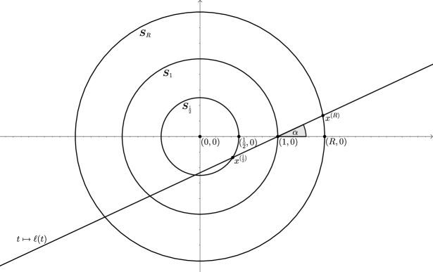
After these preparations, we turn to the martingale transports in , for as above. Figure 1 indicates a martingale transport analogous to the one constructed above in the case . Identifying again with , we define
As in the case it follows from rotational invariance that
defines a martingale transport from to . What about the invariant cells attached to the martingale transport ? Again as in the case , there are continuum many relatively open line segments
| (6.3) |
such that leaves invariant.
But now the transport is not unique any more. A striking way to see this is to replace by , i.e. mirroring the line defined in (6.2) along the -axis. In this way we obtain another martingale transport, denoted by , which is different from . In particular, the invariant cells of are obtained by “flipping” the cells in (6.3). This phenomenon is in sharp contrast to the one-dimensional setting , analyzed in [BJ16], where it was shown that the paving of into invariant cells only depends on the pair , but not on the special choice of . In the case , we refer to [GKL19] for an analysis of the invariant pavings of which do depend on the choice of , for with . In particular, our example in dimension shows that the invariant cells of a martingale transport may depend on the choice of .
The above discussion motivates the approach of [DMT19] and [OS17], which focused on the universal partition of , induced by with , as defined in [DMT19, Theorem 2.1] and revisited in Corollary 1.7 above. It turns out that in the above example of the pair , the De March–Touzi paving is in fact trivial, i.e. the pair is irreducible. More precisely, we will see that there is a Bass martingale from to , for which we have that the law of is equivalent to Lebesgue measure on the closed disk with radius in , for , while, of course, and .
We now consider the dual optimization problem for in the case , which can be explicitly solved. Let denote the uniform distribution on the sphere with radius to be specified later. Denoting by the standard Gaussian measure on , we consider the convolution measure and define the Brenier map from to . Here is a convex function on , unique up to an additive constant, for which the derivative exists Lebesgue-almost everywhere and therefore also -almost surely. As is supported by and , we have that takes its values almost surely in .
It is intuitively rather obvious that on each radial ray of , say on , the directional derivative along this ray has to take either the value or , each with conditional probability under the measure , induced on this ray. Restricting to the -axis, we obtain the following picture.
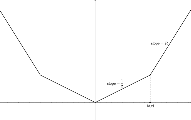
The function in Figure 2 has a kink at some point , which can be determined as the median of the conditional law of , induced on the ray . Finally we determine, for , the number as the unique number such that the rotationally invariant function maps the measure on to the measure
with barycenter . We know from the general theory that there must be a unique such for any given . It also follows from the general theory that, for , the law of is equivalent to Lebesgue measure on the closed disk with radius in , i.e.
Indeed, by [BBST23, Remark 6.3, (iii)] the law of is the image of under the map . While is equivalent to Lebesgue measure on , for , the range of is the open ball of radius on , for . In conclusion, the support of the law of is the closed disk of radius in , for .
On a last note, we discuss the limiting behaviour of the function , for . It turns out that while .
References
- [AGS08] L. Ambrosio, N. Gigli, and G. Savaré. Gradient Flows in Metric Spaces and in the Space of Probability Measures. Lect. Math. ETH Zürich. Birkhäuser, Basel, second edition, 2008.
- [Bas83] R.F. Bass. Skorokhod imbedding via stochastic integrals. In J. Azéma and M. Yor, editors, Sémin. Probab. XVII 1981/82 — Proceedings, volume of Lecture Notes in Math., pages 221–224. Springer, Berlin, Heidelberg, 1983.
- [BBHK20] J. Backhoff-Veraguas, M. Beiglböck, M. Huesmann, and S. Källblad. Martingale Benamou–Brenier: A probabilistic perspective. Ann. Probab., (5):2258–2289, 2020.
- [BBST23] J. Backhoff-Veraguas, M. Beiglböck, W. Schachermayer, and B. Tschiderer. The structure of martingale Benamou–Brenier in . arXiv:2306.11019, 2023.
- [Bee91] G. Beer. A Polish Topology for the Closed Subsets of a Polish Space. Proc. Amer. Math. Soc., (4):1123–1133, 1991.
- [BJ16] M. Beiglböck and N. Juillet. On a problem of optimal transport under marginal martingale constraints. Ann. Probab., (1):42–106, 2016.
- [BNS22] M. Beiglböck, M. Nutz, and F. Stebegg. Fine properties of the optimal Skorokhod embedding problem. J. Eur. Math. Soc., (4):1389–1429, 2022.
- [BNT17] M. Beiglböck, M. Nutz, and N. Touzi. Complete duality for martingale optimal transport on the line. Ann. Probab., (5):3038–3074, 2017.
- [Cio23a] K.J. Ciosmak. General localisation scheme I: theory. arXiv:2312.12281, 2023.
- [Cio23b] K.J. Ciosmak. General localisation scheme II: applications. arXiv:2312.13167, 2023.
- [DM78] C. Dellacherie and P.-A. Meyer. Probabilities and Potential, volume of North-Holland Mathematics Studies. North-Holland Publishing Company, Amsterdam, 1978.
- [DMT19] H. De March and N. Touzi. Irreducible convex paving for decomposition of multidimensional martingale transport plans. Ann. Probab., (3):1726–1774, 2019.
- [GKL19] N. Ghoussoub, Y.-H. Kim, and T. Lim. Structure of optimal martingale transport plans in general dimensions. Ann. Probab., (1):109–164, 2019.
- [OS17] J. Obłój and P. Siorpaes. Structure of martingale transports in finite dimensions. arXiv:1702.08433, 2017.
- [Roc70] R.T. Rockafellar. Convex analysis, volume of Princeton Mathematical Series. Princeton University Press, Princeton, NJ, 1970.
- [Str65] V. Strassen. The Existence of Probability Measures with Given Marginals. Ann. Math. Statist., (2):423–439, 1965.