Generalized FGM dependence: Geometrical representation and convex bounds on sums

Abstract

Building on the one-to-one relationship between generalized FGM copulas and multivariate Bernoulli distributions, we prove that the class of multivariate distributions with generalized FGM copulas is a convex polytope. Therefore, we find sharp bounds in this class for many aggregate risk measures, such as value-at-risk, expected shortfall, and entropic risk measure, by enumerating their values on the extremal points of the convex polytope. This is infeasible in high dimensions. We overcome this limitation by considering the aggregation of identically distributed risks with generalized FGM copula specified by a common parameter $p$. In this case, the analogy with the geometrical structure of the class of Bernoulli distribution allows us to provide sharp analytical bounds for convex risk measures.

Keywords: Multivariate Bernoulli distributions, GFGM copulas, risk measures, convex order.

1 Introduction

Finding bounds for aggregated risks with partial information on their joint distribution is a widely adressed problem in insurance and finance. The available information about dependence is often modeled using a copula. We provide analytical bounds for aggregate risks under the assumption that their dependence is modelled using a generalized Farlie-Gumbel-Morgenstern (GFGM) copula. The aim of our work is beyond the appropriateness of adopting GFGM copulas in any specific application. We study their mathematical, and geometrical properties, that make them a powerful tool to deal with aggregated risks.

With this purpose in mind, we previously find a stochastic representation that generalizes the correspondence proved in [Blier-Wong et al., 2024a] to any random vector $\boldsymbol{X}=(X_{1},\ldots,X_{d})$ with dependence structure defined by a generalized FGM copula. This representation is a one-to-one correspondence between generalized FGM copulas and multivariate Bernoulli vectors. Building on this representation we prove that the class $\mathcal{G}^{\boldsymbol{p}}_{d}(F_{1},\ldots,F_{d})$ of joint distributions of random vectors $\boldsymbol{X}$ with univariate marginals $F_{1},\dots,F_{d}$ and generalized FGM copula with parameters $\boldsymbol{p}=(p_{1},\dots,p_{d})$ is a convex polytope, that is a convex hull of a finite set of points, called extremal points. An important consequence is that many functionals $\phi(S)$, where $S=\sum_{j=1}^{d}X_{j}$, are bounded by their evaluations on the extremal points, see [Fontana and Semeraro, 2023]. However, the number of extremal points is huge and there are computational limitations in finding them in high dimensions. To overcome this limitation, we consider the class of GFGM copulas with $p_{1}=\dots=p_{d}=p$, which we call GFGM$(p)$ copulas.

We prove that the class $\mathcal{G}_{d}^{p}(F)$ of joint distributions with a common univariate margin $F$ and GFGM$(p)$ copula share the same geometrical structure of the class of multivariate Bernoulli distributions. This analogy allows us to easily work with sums $S=X_{1}+\dots+X_{d}$ of random variables with joint distribution in $\mathcal{G}_{d}^{p}(F)$, applying the results of [Fontana et al., 2021].

We also show that the convex order is preserved from the elements of the class of sums of components of random vectors following Bernoulli distributions to the class of our interest $\mathcal{S}_{d}^{p}(F)$. This contribution is important because the bounds for convex risk measures, e.g. expected shortfall, of sums in $\mathcal{S}_{d}^{p}(F)$ can be easily found by considering the random vectors that correspond to the exchangeable Bernoulli random vectors that are minimal and maximal under the (stronger) supermodular order, provided by the author of [Frostig, 2001].

We considered two convex measures of risk, the expected shortfall, and the entropic risk measure and also the value-at-risk. We analytically find their bounds in the cases of exponential margins and discrete margins and provide numerical illustrations in these two special cases in high dimensions. Building on the geometrical structure of the joint distributions behind the sums, we exhibit some possible alternative dependence structures corresponding to minimal aggregate risk. Although the theoretical investigation of this case is beyond the scope of this paper, we also discuss some numerical examples of the generalized FGM dependence, without the assumption of identically distributed risk. In this general case, we arrive up to dimension $d=5$, where we can proceed by enumeration of the extremal points. The paper is structured as follows. Section 2 introduces the preliminary notions about multivariate Bernoulli distributions and GFGM copulas with a common parameter and also their link. A new stochastic representation for GFMG copulas is proved in Section 3.2. We study the geometrical structure and the convex order in the class of uniform vectors with GFGM copulas with a common parameter $p$ in Section 4. In the subsequent section, we provide sharp bounds for the convex risk measures and the value-at-risk and we provide numerical illustrations. The last Section 6 presents an example of generalization to different values of $p$ for future research purposes and concludes.

2 Preliminaries

In this section, we recall the preliminaries on the set $\mathcal{B}_{d}$ of $d$-dimensional probability mass functions (pmfs) which have Bernoulli univariate marginal distributions and the preliminary notions on the class $\mathcal{C}_{d}$ of generalized Farlie-Gumbel-Morgenstern (GFGM) copulas.

2.1 Notation

We use the following notation throughout the paper:

• bold letters indicate vectors;

• random variables and random vectors are denoted with capital letters $X,Y,\boldsymbol{X},\boldsymbol{Y},\dots$;

• cumulative distribution functions (cdf) are denoted by $F$ and by $F_{X}$ if it is necessary to indicate the corresponding random variable or vector of random variables;

• (joint) pmfs and probability density functions (pdfs) are denoted by small letters $f,r,\dots$ and by $f_{X}$ if it is necessary to indicate the corresponding random variable or vector;

• if $f_{\boldsymbol{X}}$ is the joint pmf of $\boldsymbol{X}=(X_{1},\ldots,X_{d})$, we denote the $(j_{1},\ldots,j_{k})$-marginal pmf by $f_{\boldsymbol{X}}^{(j_{1},\ldots,j_{k})}$, that is the pmf of $(X_{j_{1}},\ldots,X_{j_{k}})$, with $1\leq j_{1}<j_{2}<\ldots<j_{k}\leq d$ and $k\in\{1,\ldots,d\}$;

• classes of (joint) pmfs or (joint) cdfs are denoted with calligraphic letters $\mathcal{F},\mathcal{B},\mathcal{G},\dots$;

• classes of copulas are denoted with the calligraphic letter $\mathcal{C}$;

• notations $X\in\mathcal{F}$ ($\boldsymbol{X}\in\mathcal{F}$), $F_{X}\in\mathcal{F}$ ($F_{\boldsymbol{X}}\in\mathcal{F}$), and $f_{X}\in\mathcal{F}$ ($f_{\boldsymbol{X}}\in\mathcal{F}$) indicate that $X$ ($\boldsymbol{X}$) has (joint) cdf, (joint) pmf or (joint) pdf in $\mathcal{F}$, respectively;

• notation $\boldsymbol{U}\in\mathcal{C}$ indicates that the joint cdf $C$ of the random vector $\boldsymbol{U}$ with uniform margins is a copula $C\in\mathcal{C}$;

• the notation $\overset{\mathcal{L}}{=}$ indicates equality in distribution.

2.2 Multivariate Bernoulli distributions and convex polytopes

Let us consider the Fréchet class $\mathcal{B}_{d}(\boldsymbol{p})=\mathcal{B}_{d}(p_{1},\ldots,p_{d})$ of multivariate Bernoulli distributions with Bernoulli marginal distributions of parameters $p_{j},j\in\{1,\ldots,d\}$. We assume throughout the paper that $p_{j}$ are rational, that is $p_{j}\in\mathbb{Q}$, $j\in\{1,\ldots,d\}$. Since $\mathbb{Q}$ is dense in $\mathbb{R}$, this is not a limitation in applications. We denote with $\mathcal{B}_{d}(p)$ the class of multivariate Bernoulli distributions with identical Bernoulli marginal distributions of parameter $p$, meaning $p_{1}=\ldots=p_{d}=p$.

If $\boldsymbol{I}=(I_{1},\dots,I_{d})$ is a random vector with joint pmf in $\mathcal{B}_{d}$, we denote the column vector which contains the values of $F$ and $f$ over $\mathcal{X}_{d}=\{0,1\}^{d}$ by $\boldsymbol{F}=(F_{\boldsymbol{x}}:\boldsymbol{x}\in\mathcal{X}_{d}):=(F(\boldsymbol{x}):\boldsymbol{x}\in\mathcal{X}_{d})$, and $\boldsymbol{f}=(f_{\boldsymbol{x}}:\boldsymbol{x}\in\mathcal{X}_{d}):=(f(\boldsymbol{x}):\boldsymbol{x}\in\mathcal{X}_{d})$, respectively; we make the non-restrictive hypothesis that the set $\mathcal{X}_{d}$ of $2^{d}$ binary vectors is ordered according to the reverse-lexicographical criterion. As an example, we consider $d=3$ and we have $\mathcal{X}_{3}=\{000,100,010,110,001,101,011,111\}$. The notations $\boldsymbol{F}\in\mathcal{B}_{d}(\boldsymbol{p})$ and $\boldsymbol{f}\in\mathcal{B}_{d}(\boldsymbol{p})$ indicate that $\boldsymbol{I}$ has joint pmf $f\in\mathcal{B}_{d}(\boldsymbol{p})$.

We assume that vectors are column vectors and we denote by $A^{\top}$ the transpose of a matrix $A$. In [Fontana and Semeraro, 2018], the authors prove that $\mathcal{B}_{d}(\boldsymbol{p})$ is a convex polytope (see as a standard reference [De Berg et al., 1997]); it means that $\mathcal{B}_{d}(\boldsymbol{p})$ admits the following representation:

$$\mathcal{B}_{d}(\boldsymbol{p})=\{\boldsymbol{f}\in\mathbb{R}_{+}^{2^{d}}:H\boldsymbol{f}=0,\sum_{\boldsymbol{x}\in\mathcal{X}_{d}}f_{\boldsymbol{x}}=1\},$$

where $H$ is a $d\times 2^{d}$ matrix whose rows, up to a non-influential multiplicative constant, are $((\boldsymbol{1}-\boldsymbol{x}_{j})^{\top}-\tfrac{(1-p_{j})}{p_{j}}\boldsymbol{x}_{j}^{\top})$, $j\in\{1,\ldots,d\}$ and where $\boldsymbol{x}_{j}$ is the vector which contains only the $j$-th element of $\boldsymbol{x}\in\mathcal{X}_{d}$, $j\in\{1,\ldots,d\}$, e.g for the bivariate case $\boldsymbol{x}_{1}^{T}=(0,1,0,1)$ and $\boldsymbol{x}_{2}^{T}=(0,0,1,1)$. Therefore, there are joint pmfs $\boldsymbol{r}_{k}\in\mathcal{B}_{d}(\boldsymbol{p})$, $k\in\{1,\ldots,n_{\boldsymbol{p}}^{\mathcal{B}}\}$, and for any $\boldsymbol{f}\in\mathcal{B}_{d}(\boldsymbol{p})$, there exist $\lambda_{1},\ldots,\lambda_{n_{\boldsymbol{p}}^{\mathcal{B}}}\geq 0$ summing up to one such that

$$\boldsymbol{f}=\sum_{k=1}^{n_{\boldsymbol{p}}^{\mathcal{B}}}\lambda_{k}\boldsymbol{r}_{k}.$$ (2.1)

We call the vectors $\boldsymbol{r}_{k}$, $k\in\{1,\ldots,n_{\boldsymbol{p}}^{\mathcal{B}}\}$, the extremal points of $\mathcal{B}_{d}(\boldsymbol{p})$, and $r_{k}$ the corresponding joint pmfs of the random vector $\boldsymbol{R}_{k}$. Here, $n_{\boldsymbol{p}}^{\mathcal{B}}$ is the number of extremal points of $\mathcal{B}_{d}(\boldsymbol{p})$ which depends on $\boldsymbol{p}$ and obviously on $d$.

For low dimension $d$, the extremal points $\boldsymbol{r}_{k}$ can be found using the software 4ti2 (see [4ti2 team, 2018]). See Example 1 as an illustration when $d=3$. However, their number $n_{\boldsymbol{p}}^{\mathcal{B}}$ increases rapidly with the dimension $d$, as discussed in Section 2 of [Fontana and Semeraro, 2024].

Example 1.

We consider the class $\mathcal{B}_{d}(\boldsymbol{p})$, with $d=3$ and $\boldsymbol{p}=(\tfrac{1}{2},\tfrac{1}{3},\tfrac{2}{3})$. In this case, the $n_{\boldsymbol{p}}^{\mathcal{B}}=12$ extremal points can be found using 4ti2. The extremal points $\boldsymbol{r}_{k}$, $k\in\{1,\ldots,12\}$, of the class $\mathcal{B}_{3}(\tfrac{1}{2},\tfrac{1}{3},\tfrac{2}{3})$ are reported in Table 1.

$\boldsymbol{x}$	$\boldsymbol{r}_{1}$	$\boldsymbol{r}_{2}$	$\boldsymbol{r}_{3}$	$\boldsymbol{r}_{4}$	$\boldsymbol{r}_{5}$	$\boldsymbol{r}_{6}$	$\boldsymbol{r}_{7}$	$\boldsymbol{r}_{8}$	$\boldsymbol{r}_{9}$	$\boldsymbol{r}_{10}$	$\boldsymbol{r}_{11}$	$\boldsymbol{r}_{12}$
(0,0,0)	0	0	0	0	0	0	$\tfrac{1}{6}$	$\tfrac{1}{6}$	$\tfrac{1}{6}$	$\tfrac{1}{3}$	$\tfrac{1}{3}$	$\tfrac{1}{4}$
(1,0,0)	0	0	$\tfrac{1}{6}$	$\tfrac{1}{3}$	$\tfrac{1}{3}$	$\tfrac{1}{4}$	0	$\tfrac{1}{6}$	$\tfrac{1}{6}$	0	0	0
(0,1,0)	0	$\tfrac{1}{3}$	0	0	0	$\tfrac{1}{12}$	$\tfrac{1}{6}$	0	0	0	0	0
(1,1,0)	$\tfrac{1}{3}$	0	$\tfrac{1}{6}$	0	0	0	0	0	0	0	0	$\tfrac{1}{12}$
(0,0,1)	$\tfrac{1}{2}$	$\tfrac{1}{6}$	$\tfrac{1}{2}$	$\tfrac{1}{6}$	$\tfrac{1}{3}$	$\tfrac{5}{12}$	0	0	$\tfrac{1}{3}$	0	$\tfrac{1}{6}$	0
(1,0,1)	$\tfrac{1}{6}$	$\tfrac{1}{2}$	0	$\tfrac{1}{6}$	0	0	$\tfrac{1}{2}$	$\tfrac{1}{3}$	0	$\tfrac{1}{3}$	$\tfrac{1}{6}$	$\tfrac{5}{12}$
(0,1,1)	0	0	0	$\tfrac{1}{3}$	$\tfrac{1}{6}$	0	$\tfrac{1}{6}$	$\tfrac{1}{3}$	0	$\tfrac{1}{6}$	0	$\tfrac{1}{4}$
(1,1,1)	0	0	$\tfrac{1}{6}$	0	$\tfrac{1}{6}$	$\tfrac{1}{4}$	0	0	$\tfrac{1}{3}$	$\tfrac{1}{6}$	$\tfrac{1}{3}$	0

Table 1: Extremal points $\boldsymbol{r}_{k}$, $k\in\{1,\ldots,12\}$, of the class $\mathcal{B}_{3}(\tfrac{1}{2},\tfrac{1}{3},\tfrac{2}{3})$.

We need to introduce the following classes of distributions since they are building blocks of one of our main results:

• class $\mathcal{E}_{d}(p)\subseteq\mathcal{B}_{d}(p)$ of exchangeable $d$-dimensional Bernoulli distributions with mean $p\in[0,1]$, we recall that $f\in\mathcal{E}_{d}(p)$ if $f\in\mathcal{B}_{d}(p)$ and $f(\boldsymbol{x})=f(\boldsymbol{x}_{\sigma})$, where $\boldsymbol{x}_{\sigma}$ is any permutation of $\boldsymbol{x}$, for every $\boldsymbol{x}\in\mathcal{X}_{d}$;

• class $\mathcal{D}_{d}(dp)$ of univariate discrete distributions with support on $\{0,1,\ldots,d\}$ and mean $dp$.

If $D$ is a discrete random variable with pmf in $\mathcal{D}_{d}(dp)$, we denote the column vector containing the values of its cdf $F_{D}$ and its pmf $f_{D}$ over $\{0,\ldots,d\}$ by $\boldsymbol{F}^{D}=(F_{1}^{D},\ldots,F_{d+1}^{D})$, and $\boldsymbol{f}^{D}=(f_{1}^{D},\ldots,f_{d+1}^{D})$, respectively. In other words, $f_{D}(k)=f_{k+1}^{D}$, $k\in\{0,1,\dots,d\}$. To simplify the notation, $\boldsymbol{f}^{D}\in\mathcal{D}_{d}(dp)$ also means that $f_{D}\in\mathcal{D}_{d}(dp)$.

According to the notation established in Section 2.1, $D\in\mathcal{D}_{d}(dp)$ or $F_{D}\in\mathcal{D}_{d}(dp)$ indicates that the discrete random variable $D$ has pmf $f_{D}\in\mathcal{D}_{d}(dp)$. The authors of [Fontana et al., 2021] prove that $\mathcal{D}_{d}(dp)$ is a convex polytope: it means that $\boldsymbol{f}^{D}\in\mathcal{D}_{d}(dp)$ if and only if there exist $\lambda_{1},\ldots,\lambda_{n_{p}^{\mathcal{D}}}\geq 0$ summing up to 1 such that

$${\boldsymbol{f}}^{D}=\sum_{k=1}^{n_{p}^{\mathcal{D}}}\lambda_{k}\boldsymbol{r}^{D}_{k},$$

where $\boldsymbol{r}^{D}_{k},\,k\in\{1,\ldots,n_{p}^{\mathcal{D}}\}$, are the extremal points of $\mathcal{D}_{d}(dp)$ and $n_{p}^{\mathcal{D}}$ is their number which depends on $p$ and obviously on $d$ (see Corollary 4.6 in [Fontana et al., 2021] for the computation of $n_{p}^{\mathcal{D}}$). We denote by ${R}^{D}_{k}$ a random variable with pmf $r_{D,k}$. The extremal points have at most two non-zero components, say $k_{1},k_{2}$ and the extremal pmfs $r_{D,k}$ for any $k\in\{1\ldots,n_{p}^{\mathcal{D}}\}$ have the following analytical expression:

$$r_{D,k}(y)=\begin{cases}\frac{k_{2}-dp}{k_{2}-k_{1}},&y=k_{1}\\ \frac{dp-k_{1}}{k_{2}-k_{1}},&y=k_{2}\\ 0,&\text{otherwise}\end{cases},$$

with $k_{1}=0,1,\ldots,k_{1}^{\vee}$, $k_{2}=k_{2}^{\wedge},k_{2}^{\wedge}+1,\ldots,d$. Note that $k_{1}^{\vee}$ is the largest integer less than $dp$ and $k_{2}^{\wedge}$ is the smallest integer greater than $dp$. If $dp$ is an integer, the pmf, given by

$$r_{D,dp}(y)=\begin{cases}1,&y=dp\\ 0,&\text{otherwise}\end{cases},$$

is also an extremal point.

In [Fontana et al., 2021], the authors show that the following relationship between classes of distributions holds:

$$\mathcal{E}_{d}(p)\leftrightarrow\mathcal{D}_{d}(dp),$$ (2.2)

that is, the class $\mathcal{D}_{d}(dp)$ has a one-to-one relationship with the class of exchangeable Bernoulli distributions $\mathcal{E}_{d}(p)$. From (2.2), it follows that given $D\in\mathcal{D}_{d}(dp)$ there is one and only one exchangeable element $\boldsymbol{I}^{e}\in\mathcal{B}_{d}(p)$ such that $\sum_{j=1}^{d}I^{e}_{j}\overset{\mathcal{L}}{=}D$. From (2.2) it follows that $\mathcal{E}_{d}(p)$ is a convex polytope and that the extremal points of $\mathcal{E}_{d}(p)$ are the exchangeable pmfs corresponding to the extremal points of $\mathcal{D}_{d}(dp)$. We denote by $\boldsymbol{e}_{k}$ extremal points or extremal pmfs of $\mathcal{E}_{d}(p)$, $k\in\{1,\ldots,n_{p}^{\mathcal{D}}\}$. We denote with $\boldsymbol{E}_{k}$ a random vector with pmf $e_{k}$. In Table 2 we provide each convex polytope with its generators.

Polytope	pmf-generator	rv-generator	number of generators
$\mathcal{B}_{d}(p)$	$\boldsymbol{r}_{k}\in\mathbb{R}^{2^{d}}$	$\boldsymbol{R}_{k}$	$n_{p}^{\mathcal{B}}$
$\mathcal{D}_{d}(dp)$	$\boldsymbol{r}_{D,k}\in\mathbb{R}^{d+1}$	$R_{D,k}$	$n_{p}^{\mathcal{D}}$
$\mathcal{E}_{d}(p)$	$\boldsymbol{e}_{k}\in\mathbb{R}^{2^{d}}$	$\boldsymbol{E}_{k}$	$n_{p}^{\mathcal{D}}$

Table 2: For each polytope of pmfs the second column provides the name of extremal points and their dimension, the third column provides the name of its corresponding random variable, and the last column the number of generators.

2.3 Bernoulli distributions and GFGM copulas

We start this section by recalling the definition of a $d$-variate FGM copula (see, e.g. Section 6.3 in [Durante and Sempi, 2015]).

Definition 2.1.

A $d$-variate FGM copula $C$ has the following expression:

$$C(u_{1},\ldots,u_{d})=\prod_{m=1}^{d}u_{m}\left(1+\sum_{k=2}^{d}\sum_{1\leq j_{1}<\dots<j_{k}\leq d}\theta_{j_{1},\dots,j_{k}}\bar{u}_{j_{1}}\cdots\bar{u}_{j_{k}}\right),$$

for $\boldsymbol{u}\in[0,1]^{d}$, where $\bar{\boldsymbol{u}}=1-\boldsymbol{u}$ and $\boldsymbol{\theta}=(\theta_{j_{1},\ldots,j_{k}}:1\leq j_{1}<\dots<j_{k}\leq d,k\in\{2,\ldots,d\})$ and  $\boldsymbol{\theta}$ belongs to the intersection of halfspaces

$$\bigg{\{}\boldsymbol{\theta}\in[-1,1]^{2^{d}-d-1}:1+\sum_{k=2}^{d}\sum_{1\leq j_{1}<\dots<j_{k}\leq d}\theta_{j_{1},\ldots,j_{k}}\epsilon_{j_{1}}\cdots\epsilon_{j_{k}}\geq 0\bigg{\}},$$

for all $\{\epsilon_{1},\ldots,\epsilon_{d}\}\in\{0,1\}^{d}$. We denote by $\mathcal{C}_{d}^{FGM}$ the class of FGM copulas.

Let $\boldsymbol{U}$ be a vector of $d$ uniformly distributed rvs with $F_{\boldsymbol{U}}=C$, where $C\in\mathcal{C}_{d}^{FGM}$. Lemma 2 of [Blier-Wong et al., 2023] provides the following stochastic representation of $\boldsymbol{U}$ in terms of $\boldsymbol{I}$ showing the one-to-one correspondence between $\mathcal{C}_{d}^{FGM}$ and $\mathcal{B}_{d}(\frac{1}{2})$ :

$$\boldsymbol{U}\overset{\mathcal{L}}{=}(\boldsymbol{1}-\boldsymbol{I})\boldsymbol{V}_{1}+\boldsymbol{I}\boldsymbol{V}_{2},$$ (2.3)

where $\boldsymbol{V}_{j}=(V_{j,1},\dots,V_{j,d})$ is a vector of $d$ independent and identically distributed (iid) random variables satisfying $V_{j,k}\sim Beta(j,3-j)$ for $k\in\{1,\ldots,d\}$ and $j\in\{1,2\}$ (see also [Blier-Wong et al., 2022b]).

In [Blier-Wong et al., 2024a], a class of generalized FGM copulas is introduced, building on a new stochastic representation. Let $\boldsymbol{I}\in\mathcal{B}_{d}(\boldsymbol{p})$ be a $d$-variate Bernoulli random vector. Let $\boldsymbol{U}_{0}=(U_{0,1},\dots,U_{0,d})$ and $\boldsymbol{U}_{1}=(U_{1,1},\dots,U_{1,d})$ be vectors of $d$ independent uniform rvs. The random vectors $\boldsymbol{I}$, $\boldsymbol{U}_{0}$ and $\boldsymbol{U}_{1}$ are independent of each other. Further, define the representation

$$\boldsymbol{U}\overset{\mathcal{L}}{=}\boldsymbol{U}_{0}^{{1}-{\boldsymbol{p}}}\boldsymbol{U}_{1}^{\boldsymbol{I}}=(U_{0,1}^{1-p_{1}}U_{1,1}^{I_{1}},\dots,U_{0,d}^{1-p_{d}}U_{1,d}^{I_{d}}).$$ (2.4)

In [Blier-Wong et al., 2024a], the authors show that the joint cdf of the random vector in (2.4) is the generalized FGM copula provided in the following definition.

Definition 2.2.

A $d$-variate generalized FGM (GFGM) copula $C$ with vector of parameters $\boldsymbol{p}=(p_{1},\ldots,p_{d})$ has the following expression

$$C(\boldsymbol{u})=\prod_{m=1}^{d}u_{m}\left(1+\sum_{k=2}^{d}\sum_{1\leq j_{1}<\dots<j_{k}\leq d}\nu_{j_{1}\dots j_{k}}\left(1-u_{j_{1}}^{\frac{p_{j_{1}}}{1-p_{j_{1}}}}\right)\cdots\left(1-u_{j_{k}}^{\frac{p_{j_{k}}}{1-p_{j_{k}}}}\right)\right),$$

for $\boldsymbol{u}\in[0,1]^{d},$ where, for $1\leq j_{1}<\dots<j_{k}\leq d,k\in\{2,\dots,d\}$,

$$\nu_{j_{1}\dots j_{k}}=\mathrm{E}\left[\prod_{n=1}^{k}\frac{I_{j_{n}}-p_{j_{n}}}{p_{j_{n}}}\right],$$

where $\boldsymbol{I}=(I_{1},\dots,I_{d})\in\mathcal{B}_{d}(\boldsymbol{p})$.

We denote by $\mathcal{C}_{d}$ the class of generalized FGM (GFGM) copulas. We use the notation $\mathcal{C}_{d}^{\boldsymbol{p}}$ or $\mathcal{C}_{d}^{p}$ to indicate the subclasses of GFGM copulas with parameters $\boldsymbol{p}=(p_{1},\ldots,p_{d})$ or with a common parameter $p$. In the special case $p=\tfrac{1}{2}$, $\mathcal{C}_{d}^{1/2}\equiv\mathcal{C}_{d}^{\text{FGM}}$, where $\mathcal{C}_{d}^{\text{FGM}}$ is the class of FGM copulas, and the stochastic representations in (2.4) and (2.3) are equivalent.

Example 1 (continued).

In Table 3, we provide the values of the four parameters $\nu_{1,2}$, $\nu_{1,3}$, $\nu_{2,3}$, and $\nu_{1,2,3}$ of $n_{\boldsymbol{p}}^{\mathcal{B}}=12$ extremal copulas $C_{\boldsymbol{R}_{k}}$, $k\in\{1,\ldots,12\}$, of the class $\mathcal{C}_{3}^{\boldsymbol{p}}$ of trivariate GFGM copulas with $\boldsymbol{p}=(\tfrac{1}{2},\tfrac{1}{3},\tfrac{2}{3})$.

	$C_{\boldsymbol{R}_{1}}$	$C_{\boldsymbol{R}_{2}}$	$C_{\boldsymbol{R}_{3}}$	$C_{\boldsymbol{R}_{4}}$	$C_{\boldsymbol{R}_{5}}$	$C_{\boldsymbol{R}_{6}}$	$C_{\boldsymbol{R}_{7}}$	$C_{\boldsymbol{R}_{8}}$	$C_{\boldsymbol{R}_{9}}$	$C_{\boldsymbol{R}_{10}}$	$C_{\boldsymbol{R}_{11}}$	$C_{\boldsymbol{R}_{12}}$
$\nu_{1,2}$	$1$	$-1$	$1$	$-1$	$0$	$\tfrac{1}{2}$	$-1$	$-1$	$1$	$0$	$1$	$-\tfrac{1}{2}$
$\nu_{1,3}$	$-\tfrac{1}{2}$	$\tfrac{1}{2}$	$-\tfrac{1}{2}$	$-\tfrac{1}{2}$	$-\tfrac{1}{2}$	$-\tfrac{1}{4}$	$\tfrac{1}{2}$	0	0	$\tfrac{1}{2}$	$\tfrac{1}{2}$	$\tfrac{1}{4}$
$\nu_{2,3}$	$-1$	$-1$	$-\tfrac{1}{4}$	$\tfrac{1}{2}$	$\tfrac{1}{2}$	$\tfrac{1}{8}$	$-\tfrac{1}{4}$	$\tfrac{1}{2}$	$\tfrac{1}{2}$	$\tfrac{1}{2}$	$\tfrac{1}{2}$	$\tfrac{1}{8}$
$\nu_{1,2,3}$	$-\tfrac{1}{2}$	$\tfrac{1}{2}$	$\tfrac{1}{4}$	$0$	$\tfrac{1}{2}$	$\tfrac{7}{8}$	$-\tfrac{1}{4}$	$-\tfrac{1}{2}$	$\tfrac{1}{2}$	$-\tfrac{1}{2}$	$0$	$-\tfrac{7}{8}$

Table 3: Parameters of the $n_{\boldsymbol{p}}^{\mathcal{B}}=12$ extremal copulas $C_{\boldsymbol{R}_{j}}$, $j\in\{1,\ldots,12\}$, of the class $\mathcal{C}_{3}^{\boldsymbol{p}}$ of trivariate GFGM copulas with $\boldsymbol{p}=(\tfrac{1}{2},\tfrac{1}{3},\tfrac{2}{3})$.

3 Geometrical structure of GFGM$(\boldsymbol{p})$ copulas

In [Blier-Wong et al., 2024a], the authors mention in Remark 1 that the class $\mathcal{C}^{\boldsymbol{p}}_{d}$ shares the geometrical structure of $\mathcal{B}_{d}(\boldsymbol{p})$. In particular, any $F_{\boldsymbol{U}}\in\mathcal{C}_{d}^{\boldsymbol{p}}$ is a convex combination of $F_{\boldsymbol{U}^{(\boldsymbol{R}_{k})}}$, where $\boldsymbol{U}^{(\boldsymbol{R}_{k})}$ is built from $\boldsymbol{R}_{k}$ according to (2.4), $k\in\{1,\ldots,n_{\boldsymbol{p}}^{\mathcal{B}}\}$. Indeed, by using the stochastic representation in (2.4), there is $\boldsymbol{I}\in\mathcal{B}_{d}(\boldsymbol{p})$ such that $\boldsymbol{U}=\boldsymbol{U}^{(\boldsymbol{I})}=\boldsymbol{U}_{0}^{{1}-{\boldsymbol{p}}}\boldsymbol{U}_{1}^{\boldsymbol{I}}$, and we have

$$\begin{split}F_{\boldsymbol{U}^{(\boldsymbol{I})}}(\boldsymbol{x})&=\Pr\bigg{(}U_{1}^{(\boldsymbol{I})}\leq x_{1},\ldots,U_{d}^{(\boldsymbol{I})}\leq x_{d}\bigg{)}=\Pr\bigg{(}U_{0,1}^{1-p_{1}}U_{1,1}^{I_{1}}\leq x_{1},\ldots,U_{0,d}^{1-p_{d}}U_{1,d}^{I_{d}}\leq x_{d}\bigg{)}\\ &\overset{*}{=}\sum_{\boldsymbol{j}\in\{0,1\}^{d}}\Pr\bigg{(}U_{0,1}^{1-p_{1}}U_{1,1}^{i_{1}}\leq x_{1},\ldots,U_{0,d}^{1-p_{d}}U_{1,d}^{i_{d}}\leq x_{d}\bigg{)}f_{\boldsymbol{I}}(\boldsymbol{j})\\ &=\sum_{k=1}^{n_{p}^{\mathcal{B}}}\lambda_{k}\sum_{\boldsymbol{j}\in\{0,1\}^{d}}\Pr\bigg{(}U_{0,1}^{1-p_{1}}U_{1,1}^{i_{1}}\leq x_{1},\ldots,U_{0,d}^{1-p_{d}}U_{1,d}^{i_{d}}\leq x_{d}\bigg{)}r_{k}(\boldsymbol{j})\\ &\overset{**}{=}\sum_{k=1}^{n_{p}^{\mathcal{B}}}\lambda_{k}\Pr\bigg{(}U_{0,1}^{1-p_{1}}U_{1,1}^{R_{k,1}}\leq x_{1},\ldots,U_{0,d}^{1-p_{d}}U_{1,d}^{R_{k,d}}\leq x_{d}\bigg{)}\\ &=\sum_{k=1}^{n_{p}^{\mathcal{B}}}\lambda_{k}F_{\boldsymbol{U}^{(\boldsymbol{R}_{k})}}(\boldsymbol{x}),\qquad\boldsymbol{x}\in[0,1]^{d},\end{split}$$

where equalities $\overset{*}{=}$ and $\overset{**}{=}$ follow from the independence of $\boldsymbol{U}_{0}$, $\boldsymbol{U}_{1}$ and $\boldsymbol{I}$ and of $\boldsymbol{U}_{0}$, $\boldsymbol{U}_{1}$ and $\boldsymbol{R}_{k}$, $k\in\{1,\ldots,n_{\boldsymbol{p}}^{\mathcal{B}}\}$. It follows that any GFGM copula $C$ admits the representation

$$C(\boldsymbol{u})=\sum_{k=1}^{n_{\boldsymbol{p}}^{\mathcal{B}}}\lambda_{k}C_{\boldsymbol{R}_{k}}(\boldsymbol{u}),\quad\boldsymbol{u}\in[0,1]^{d},$$ (3.1)

where $C_{\boldsymbol{R}_{k}}$ is the copula associated to $\boldsymbol{U}^{(\boldsymbol{R}_{k})}$, $k\in\{1,\ldots,n_{\boldsymbol{p}}^{\mathcal{B}}\}$. The class $\mathcal{C}_{d}^{\boldsymbol{p}}$ of copulas is a convex polytope.

Example 1 (continued).

Any copula $C\in\mathcal{C}_{d}^{\boldsymbol{p}}$ with $\boldsymbol{p}=(p_{1},p_{2},p_{3})$ has the following expression:

$$\begin{split}C(\boldsymbol{u})&=u_{1}u_{2}u_{3}\bigg{(}1+\nu_{1,2}\left(1-u_{1}^{\frac{p_{1}}{1-p{1}}}\right)\left(1-u_{2}^{\frac{p_{2}}{1-p{2}}}\right)+\nu_{1,3}\left(1-u_{1}^{\frac{p_{1}}{1-p{1}}}\right)\left(1-u_{3}^{\frac{p_{3}}{1-p{3}}}\right)+\\ &+\nu_{2,3}\left(1-u_{2}^{\frac{p_{2}}{1-p{2}}}\right)\left(1-u_{3}^{\frac{p_{3}}{1-p{3}}}\right)+\nu_{1,2,3}\left(1-u_{1}^{\frac{p_{1}}{1-p{1}}}\right)\left(1-u_{2}^{\frac{p_{2}}{1-p{2}}}\right)\left(1-u_{3}^{\frac{p_{3}}{1-p{3}}}\right)\bigg{)},\end{split}$$

for $\boldsymbol{u}=(u_{1},u_{2},u_{3})\in[0,1]^{3}.$ If $\boldsymbol{p}=(\tfrac{1}{2},\tfrac{1}{3},\tfrac{2}{3})$, any copula $C\in\mathcal{C}_{3}^{\boldsymbol{p}}$ can be expressed as the linear convex combination in (3.1) of the twelve ($n^{\mathcal{B}}_{\boldsymbol{p}}=12$) extremal copulas with parameters in Table 3.

3.1 Class $\mathcal{G}_{d}^{\boldsymbol{p}}(F_{1},\dots,F_{d})$ of distributions

We provide in the proposition that follows a general result for a class of multivariate distributions with dependence structure built with a family of copulas being a convex polytope. Our aim is to later investigate the specific class $\mathcal{G}_{d}^{\boldsymbol{p}}(F_{1},\dots,F_{d})$ of distributions with marginal distributions $F_{1},\ldots,F_{d}$ and with copula in the class $\mathcal{C}_{d}^{\boldsymbol{p}}$.

Proposition 3.1.

Let $\mathcal{C}$ be a class of copulas. Let $\mathcal{F}_{d}(F_{1},\dots,F_{d})$ be a class of multivariate distributions with marginal distributions $F{{}_{1}},\ldots,F{{}_{d}}$ and with copula in the class $\mathcal{C}$. If $\mathcal{C}$ is a convex polytope with extremal points $\widetilde{C}_{1},...,\widetilde{C}_{n}$, then $\mathcal{F}_{d}(F_{1},\dots,F_{d})$ is a convex polytope with extremal points $\widetilde{F}_{1},...,\widetilde{F}_{n}$, where

$$\widetilde{F}_{i}(\boldsymbol{x})=\widetilde{C}_{i}(F_{1}(x_{1}),...,F_{d}(x_{d}))$$

for every $\boldsymbol{x}\in\mathbb{R}^{d}$ and $i\in\{1,\ldots,n\}$.

Proof.

Consider $F_{\boldsymbol{X}}\in\mathcal{F}_{d}(F_{1},\dots,F_{d})$. Then, for $\boldsymbol{x}\in\mathbb{R}^{d}$, we have

$$F_{\boldsymbol{X}}(\boldsymbol{x}) =C(F_{1}(x_{1}),...,F_{d}(x_{d}))$$

$$=\sum_{i=1}^{n}\lambda_{i}\widetilde{C}_{i}(F_{1}(x_{1}),...,F_{d}(x_{d})),$$

for some $\lambda_{1},...,\lambda_{n}\geq 0$ such that $\sum_{i=1}^{n}\lambda_{i}=1$. Define $\widetilde{F}_{i}(\boldsymbol{x})=\widetilde{C}_{i}(F_{1}(x_{1}),...,F_{d}(x_{d}))$ and the desired result directly follows. ∎

Corollary 3.1.

The class $\mathcal{G}_{d}^{\boldsymbol{p}}(F_{1},\dots,F_{d})$ of distributions is a convex polytope with extremal points the distributions associated to the extremal points $\boldsymbol{r}_{k}$ of $\mathcal{B}_{d}(\boldsymbol{p})$, $k\in\{1,\ldots,n^{\mathcal{B}}_{\boldsymbol{p}}\}$.

3.2 A new representation theorem and consequences

We introduce a stochastic representation for any random vector $\boldsymbol{X}$ with distribution in $\mathcal{G}_{d}^{\boldsymbol{p}}(F_{1},\dots,F_{d})$. We then use this representation in two particular cases, more precisely with exponential and discrete marginals for which the expression of the distribution of the sum is analytical.

Theorem 3.1.

Fix some margins $F_{1},\ldots,F_{d}$ and, for $h\in\{0,1\}$, let $\boldsymbol{Z}_{h}=(Z_{h,1},\ldots,Z_{h,d})$ be vectors of independent random variables with $Z_{0,j}\overset{\mathcal{L}}{=}F^{-1}_{j}(V_{0})$ and $Z_{1,j}\overset{\mathcal{L}}{=}F^{-1}_{j}(V_{1}V_{0})$, for all $j\in\{1,\ldots,d\}$, where $V_{0}\sim Beta\left(\frac{1}{1-p},1\right)$ and $V_{1}\sim U(0,1)$ and let them be independent. Define the random vector

$$\boldsymbol{X}=(\boldsymbol{1}-\boldsymbol{I})\boldsymbol{Z}_{0}+\boldsymbol{I}\boldsymbol{Z}_{1},$$ (3.2)

where $\boldsymbol{I}\in\mathcal{B}_{d}(\boldsymbol{p})$. Then we have $F_{\boldsymbol{X}}\in\mathcal{G}_{d}^{\boldsymbol{p}}(F_{1},\ldots,F_{d})$, that is the distribution of the random vector $\boldsymbol{X}$ has margins $F_{1},\dots,F_{d}$ and copula $C\in\mathcal{C}_{d}^{\boldsymbol{p}}$.

Proof.

Let $\boldsymbol{U}\in\mathcal{C}_{d}^{\boldsymbol{p}}$ and hence $\boldsymbol{U}=\boldsymbol{U}_{0}^{1-\boldsymbol{p}}\boldsymbol{U}^{\boldsymbol{I}}$, where $\boldsymbol{I}\in\mathcal{B}_{d}(\boldsymbol{p})$, with $\boldsymbol{p}=(p_{1},\dots,p_{d})$. In the proof of Theorem 2 in [Blier-Wong et al., 2024a], we have

$$F_{U_{j}}(u)=\Pr(U_{0,j}^{1-p_{j}}U_{1,j}^{I_{j}}\leq u)=\Pr(I_{j}=0)F_{U_{j}|I_{j}=0}(u)+\Pr(I_{j}=1)F_{U_{j}|I_{j}=1}(u),$$

where

$$F_{U_{j}|I_{j}=0}(u)=u^{\frac{1}{1-p_{j}}}$$

and

$$F_{U_{j}|I_{j}=1}(u)=\frac{u}{p_{j}}-\frac{1-p_{j}}{p_{j}}u^{\frac{1}{1-p_{j}}},\quad j\in\{1,\ldots,d\}.$$

Thus $(U_{j}|I_{j}=0)\overset{\mathcal{L}}{=}V_{0}$ and $(U_{j}|I_{j}=1)\overset{\mathcal{L}}{=}V_{0}V_{1}$, $j\in\{1,\ldots,d\}$, and the assert follows. ∎

Obviously, the special case of uniform margins leads to a stochastic representation of the GFGM family of copulas similar to (2.3) and equivalent to (2.4). We notice that for $p=\tfrac{1}{2}$ we find the stochastic representation of FGM copulas in [Blier-Wong et al., 2024b].

Theorem 3.1 provides a very useful representation of the random vector $\boldsymbol{X}$. This helps us to derive plenty of results such as examining the distribution of any integrable function of $\boldsymbol{X}$ and analyzing pairwise dependence properties of $\boldsymbol{X}$. The following corollary considers the expectation of functionals of $\boldsymbol{X}$ for which we derive bounds, in Section 5, building on the geometrical structure of Bernoulli vectors, the distribution of the sum $S^{(\boldsymbol{X})}=X_{1}+\dots+X_{d}$ which may represent aggregate risks in a portfolio and some results on correlation between components of $\boldsymbol{X}$ to analyze dependence corresponding to minimal aggregate risks.

Corollary 3.2.

Let $\boldsymbol{X}\in\mathcal{G}^{\boldsymbol{p}}_{d}(F_{1},\ldots,F_{d})$, and let $r_{k}$, $k\in\{1,\dots,n_{\boldsymbol{p}}^{\mathcal{B}}\}$, be the extremal pmfs of $\mathcal{B}_{d}(\boldsymbol{p})$. The following holds.

1. Let $\varphi\colon\mathbb{R}^{d}\to\mathbb{R}$ be a real-valued function for which the expectation exists, we have

   $$E[\varphi(X_{1},\dots,X_{d})] =\sum_{k=1}^{n_{\boldsymbol{p}}^{\mathcal{B}}}\lambda_{k}\sum_{\boldsymbol{i}\in\{0,1\}^{d}}r_{k}(\boldsymbol{i})E[\varphi(Z_{i_{1},1},\dots,Z_{i_{d},d})],$$ (3.3)

2. The distribution of the sum $S=\sum_{j}^{d}X_{j}$ is given by

   $$F_{S}(y)=\sum_{k=1}^{n_{p}^{\mathcal{B}}}\lambda_{k}\sum_{\boldsymbol{i}\in\{0,1\}^{d}}r_{k}(\boldsymbol{i})F_{\sum_{j=1}^{d}Z_{i_{j},j}}(y),\quad y\in\mathbb{R}.$$ (3.4)

3. The covariance between each pair of components $(X_{j_{1}},X_{j_{2}})$ of $\boldsymbol{X}$, $1\leq j_{1}<j_{2}\leq d$, is:

   $$Cov(X_{j_{1}},X_{j_{2}})=Cov(I_{j_{1}},I_{j_{2}})(E[Z_{1,j_{1}}]-E[Z_{0,j_{1}}])(E[Z_{1,j_{2}}]-E[Z_{0,j_{2}}]),$$ (3.5)

   and if $\boldsymbol{X}$ has continuous marginal distributions, Spearman’s rho between each pair of components $(X_{j_{1}},X_{j_{2}})$ of $\boldsymbol{X}$, $1\leq j_{1}<j_{2}\leq d$, is:

   $$\rho_{S}(X_{j_{1}},X_{j_{2}}) =\frac{3\,Cov(I_{j_{1}},I_{j_{2}})}{(2-p_{j_{1}})(2-p_{j_{2}})},$$

   where $\boldsymbol{I}=(I_{1},\dots,I_{d})$ is the Bernoulli random vector corresponding to $\boldsymbol{X}$ of Theorem 3.1. The sharp bounds of the Spearman’s rho are:

   $$\frac{3(\max(p_{j_{1}}+p_{j_{2}}-1,0)-p_{j_{1}}p_{j_{2}})}{(2-p_{j_{1}})(2-p_{j_{2}})}\leq\rho_{S}(X_{j_{1}},X_{j_{2}})\leq\frac{3p_{j_{1}}(1-p_{j_{2}})}{(2-p_{j_{1}})(2-p_{j_{2}})},$$

Proof.

From the stochastic representation in (3.2) of Theorem 3.1, we have

$$X_{j}=\begin{cases}Z_{1,j}\,\,\,&\text{if }I_{j}=1\\ Z_{0,j}\,\,\,&\text{if }I_{j}=0\end{cases}.$$

Thus, $X_{j}=Z_{I_{j}.j}$ and by conditioning on $\boldsymbol{I}$, the expectation of a function $\varphi$ of $\boldsymbol{X}$ is given by

$$E[\varphi(X_{1},\dots,X_{d})] =\sum_{\boldsymbol{i}\in\{0,1\}^{d}}f_{\boldsymbol{I}}(\boldsymbol{i})E[\varphi(Z_{i_{1},1},\dots,Z_{i_{d},d})],$$ (3.6)

assuming that the expectations exist.

1. By replacing (2.1) in (3.6), (3.3) follows.

2. By choosing $\varphi(\boldsymbol{x})=\boldsymbol{1}\{x_{1}+\dots+x_{d}\leq y\}$, where $\boldsymbol{1}\{A\}=1$, if $A$ is true, and $\boldsymbol{1}\{A\}=0$, otherwise, (3.4) follows.

3. Covariance between $X_{j_{1}}$ and $X_{j_{2}}$ in (3.5), $1\leq j_{1}<j_{2}\leq d$, follows by considering $\varphi(\boldsymbol{x})=x_{j_{1}}x_{j_{2}}$ in (3.6).

   Spearman’s rho $\rho_{S}$ for any pair of continuous rvs $(X_{j_{1}},X_{j_{2}})$, $1\leq j_{1}<j_{2}\leq d$, is given by

   $$\rho_{S}(X_{j_{1}},X_{j_{2}})=\rho_{P}(U_{j_{1}},U_{j_{2}})=\frac{E[U_{j_{1}}U_{j_{2}}]-E[U_{j_{1}}]E[U_{j_{2}}]}{\sqrt{Var(U_{j_{1}})Var(U_{j_{2}})}},$$ (3.7)

   where $\rho_{P}$ indicates the Pearson’s correlation and $Var(U_{j_{1}})=Var(U_{j_{2}})=\frac{1}{12}$. Using the representation in (2.4), the expression for $E[U_{j_{1}}U_{j_{2}}]$, $1\leq j_{1}<j_{2}\leq d$, is

   $$E[U_{j_{1}}U_{j_{2}}]=E[U_{0,j_{1}}^{1-{p_{j_{1}}}}U_{0,j_{2}}^{1-p_{j_{2}}}U_{1,j_{1}}^{I_{j_{1}}}U_{1,j_{2}}^{I_{j_{2}}}]=E[U_{0,j_{1}}^{1-p_{j_{1}}}]E[U_{0,j_{2}}^{1-p_{j_{2}}}]E[U_{1,j_{1}}^{I_{j_{1}}}U_{1,j_{2}}^{I_{j_{2}}}],$$

   where

   $$E[U_{0,j_{1}}^{1-p}]E[U_{0,j_{2}}^{1-p}]=\frac{1}{2-p_{j_{1}}}\frac{1}{2-p_{j_{2}}}$$

   and

   $$E[U_{1,j_{1}}^{I_{j_{1}}}U_{1,j_{2}}^{I_{j_{2}}}] =\sum_{(i_{j_{1}},i_{j_{2}})\in\{0,1\}^{2}}f_{\boldsymbol{I}}^{(j_{1},j_{2})}(i_{j_{1}},i_{j_{2}})E[U_{1,j_{1}}^{i_{j_{1}}}]E[U_{1,j_{2}}^{i_{j_{2}}}].$$ (3.8)

   Finally, replacing (3.8) in (3.7), the expression of the Spearman’s rho is given by

   $$\rho_{S}(X_{j_{1}},X_{j_{2}}) =\frac{12f_{\boldsymbol{I}}^{(j_{1},j_{2})}(0,0)+6(f_{\boldsymbol{I}}^{(j_{1},j_{2})}(0,1)+f_{\boldsymbol{I}}^{(j_{1},j_{2})}(1,0))+3f_{\boldsymbol{I}}^{(j_{1},j_{2})}(1,1)}{(2-p_{j_{1}})(2-p_{j_{2}})}-3$$

   $$=\frac{3(f_{\boldsymbol{I}}^{(j_{1},j_{2})}(1,1)-p_{1}p_{2})}{(2-p_{j_{1}})(2-p_{j_{2}})}$$

   $$=\frac{3\,Cov(I_{j_{1}},I_{j_{2}})}{(2-p_{j_{1}})(2-p_{j_{2}})},$$

   for $1\leq j_{1}<j_{2}\leq d$.

   Assume $p_{j_{1}}\leq p_{j_{2}}$. In Section 3.2 of [Fontana and Semeraro, 2018], the authors found the bounds for the covariance between $(I_{j_{1}},I_{j_{2}})$ for any pair of Bernoulli variables. The maximum value is $Cov(I_{j_{1}},I_{j_{2}})=p_{j_{1}}(1-p_{j_{2}})$, while the minimum value is $Cov(I_{j_{1}},I_{j_{2}})=\max(p_{j_{1}}+p_{j_{2}}-1,0)-p_{j_{1}}p_{j_{2}}$. In the first case, $E[I_{j_{1}}I_{j_{2}}]=\Pr(I_{j_{1}}=1,I_{j_{2}}=1)=p_{j_{1}}$ and $Cov(I_{j_{1}},I_{j_{2}})=p_{j_{1}}(1-p_{j_{2}})$. In the second case, $E[I_{j_{1}}I_{j_{2}}]=\Pr(I_{j_{1}}=1,I_{j_{2}}=1)=\max(p_{j_{1}}+p_{j_{2}}-1,0)$ and $Cov(I_{j_{1}},I_{j_{2}})=\max(p_{j_{1}}+p_{j_{2}}-1,0)-p_{j_{1}}p_{j_{2}}$. Therefore, we have the following bounds for Spearman’s rho of any pair of continuous rvs

   $$\frac{3(\max(p_{j_{1}}+p_{j_{2}}-1,0)-p_{j_{1}}p_{j_{2}})}{(2-p_{j_{1}})(2-p_{j_{2}})}\leq\rho_{S}(X_{j_{1}},X_{j_{2}})=\rho_{P}(U_{j_{1}},U_{j_{2}})\leq\frac{3p_{j_{1}}(1-p_{j_{2}})}{(2-p_{j_{1}})(2-p_{j_{2}})},$$

   for $1\leq j_{1}<j_{2}\leq d$.

∎

Equation (3.3) in particular holds for $\phi(S^{(\boldsymbol{X})})=\varphi(\boldsymbol{X})$ and implies that the bounds of $E[\phi(S^{(\boldsymbol{X})})]$, for any $\phi$ for which the expectation exists, can be found by enumerating their values on the sums $S^{(\boldsymbol{R}_{k})},$ $k\in\{1,\ldots,n_{p}^{\mathcal{B}}\}$, and this is computationally feasible in low dimension.

3.3 Discrete and exponential margins

We end this section considering two examples for $\mathcal{G}^{\boldsymbol{p}}_{d}(F_{1},\ldots,F_{d})$, where the margins are discrete in the first one and the margins are exponential in the second one.

Example 2 (Discrete margins).

Let $\boldsymbol{X}=(X_{1},\ldots,X_{d})$ be defined here as a $d$-dimensional random vector, where, for every $j\in\{1,\ldots,d\}$, $X_{j}$ is a discrete random variable taking values on the set $A_{j}=\{0,1,\ldots,n_{j}\}$, $n_{j}\in\mathbb{N}$, and with cdf $F_{j}$. When the joint distribution of $\boldsymbol{X}$ belongs to the class $\mathcal{G}^{\boldsymbol{p}}_{d}(F_{1},\ldots,F_{d})$, $\boldsymbol{X}$ admits the representation in (3.2). Moreover, for all $j\in\{1,\ldots,d\}$, to derive the values of the pmf of the discrete rvs $Z_{i,j},\,i=0,1$, we observe that, for each $k\in A_{j}$, we have

$$f_{Z_{0,j}}(k)=\Pr(Z_{0,j}=k)=\Pr(F_{j}^{-1}(V_{0})=k)=F_{V_{0},j}(F_{j}(k))-F_{V_{0},j}(F_{j}(k-1))$$

and

$$f_{Z_{1,j}}(k)=\Pr(Z_{1,j}=k)=\Pr(F_{j}^{-1}(V_{0}V_{1})=k)=F_{V_{0}V_{1},j}(F_{j}(k))-F_{V_{0}V_{1},j}(F_{j}(k-1)),$$

where

$$F_{V_{0},j}(u)=u^{\frac{1}{1-p_{j}}},\quad u\in(0,1),$$

$$F_{V_{0}V_{1},j}(u)=\frac{u}{p_{j}}-\frac{1-p_{j}}{p_{j}}u^{\frac{1}{1-p_{j}}},\quad u\in(0,1),$$

and $F_{j}(-1):=0$. For all $j\in\{1,\ldots,d\}$, it follows that the expectations of the discrete rvs $Z_{i,j},\,i=0,1$, are

$$E[Z_{0,j}]=n_{j}-\sum_{k=0}^{n_{j}-1}F_{V_{0},j}(F_{j}(k))$$

and

$$E[Z_{1,j}]=n_{j}-\sum_{k=0}^{n_{j}-1}F_{V_{0}V_{1},j}(F_{j}(k)).$$

Finally, we consider the sum $S^{(\boldsymbol{X})}=X_{1}+\cdots+X_{d}$, which can be rewritten using the representation in (3.2), as

$$S^{(\boldsymbol{X})}=\sum_{j=1}^{d}(1-I_{j})Z_{0,j}+I_{j}Z_{1,j}.$$ (3.9)

From (3.9), the expression of the probability generating function (pgf) of $S^{(\boldsymbol{X})}$ is given by

$$\mathcal{P}_{S^{(\boldsymbol{X})}}(s)=\sum_{\boldsymbol{i}\in\{0,1\}^{d}}f_{\boldsymbol{I}}(\boldsymbol{i})\prod_{j=1}^{d}\mathcal{P}_{Z_{i_{j},j}}(s),\quad s\in[-1,1],$$ (3.10)

where the pgf of $Z_{i_{j},j}$ is

$$\mathcal{P}_{Z_{i_{j},j}}(s)=E[s^{Z_{i_{j},j}}]=\sum_{k=0}^{n_{j}}f_{Z_{i_{j},j}}(k)s^{k},\quad s\in[-1,1],$$

for $i_{j}\in\{0,1\}$ and $j\in\{1,\dots,d\}$. One uses the Fast Fourier Transform (FFT) algorithm of [Cooley and Tukey, 1965] to extract the values of the pmf of $S^{(\boldsymbol{X})}$ from its pgf in $\eqref{eq:PfgSdiscrete}$. Details about that efficient approach is explained in Chapter 30 of [Cormen et al., 2009]. See also [Embrechts et al., 1993] for FFT applications in actuarial science and quantitative risk management. This procedure is illustrated in Example 7, within Section 6. ∎

Example 3 (Exponential margins).

Assume that $\boldsymbol{X}\in\mathcal{G}^{\boldsymbol{p}}_{d}(F_{1},\ldots,F_{d})$, where $F_{j}$ is the cdf of an exponential distribution with mean $\frac{1}{\lambda_{j}}$, $j\in\{1,\ldots,d\}$. In [Blier-Wong et al., 2024a], they present an alternative stochastic representation of $\boldsymbol{X}$ equivalent to (3.2) that allows finding an analytical expression for the distribution of the sum of the components of the random vector $\boldsymbol{X}$. This other stochastic representation is

$$\boldsymbol{X}=\boldsymbol{W}_{1}+\boldsymbol{I}\boldsymbol{W}_{2},$$ (3.11)

where the components $W_{1,j}$ within $\boldsymbol{W}_{1}$ and $W_{2,j}$ within $\boldsymbol{W}_{2}$ are independent, with $W_{1,j}$ following an exponential distribution with mean $\frac{1-p_{j}}{\lambda_{j}}$ and $W_{2,j}$ also following an exponential distribution but with mean $\frac{1}{\lambda_{j}}$, for $j\in\{1,\ldots,d\}$. Also, the random vectors $\boldsymbol{I}$, $\boldsymbol{W}_{1}$ and $\boldsymbol{W}_{2}$ are independent.

From (3.11), Pearson’s coefficient becomes

$$\rho_{P}(X_{j_{1}},X_{j_{2}})=\frac{Cov(I_{j_{1}},I_{j_{2}})E[W_{2,j_{1}}]E[W_{2,j_{2}}]}{\sqrt{Var(X_{j_{1}})Var(X_{j_{2}})}}=Cov(I_{j_{1}},I_{j_{2}})$$ (3.12)

since $E[X_{j_{1}}]=\frac{1}{\lambda_{j_{1}}}$, $E[X_{j_{2}}]=\frac{1}{\lambda_{j_{2}}}$, $Var(X_{j_{1}})=\frac{1}{\lambda_{j_{1}}^{2}}$, and $Var(X_{j_{2}})=\frac{1}{\lambda_{j_{2}}^{2}}$, $1\leq j_{1}<j_{2}\leq d$.

Considering now the sum $S^{(\boldsymbol{X})}$ of the components of $\boldsymbol{X}$, the representation in (3.11) allows us to express it as follows:

$$S^{(\boldsymbol{X})}\overset{\mathcal{L}}{=}W_{1,1}+I_{1}W_{2,1}+\ldots+W_{1,d}+I_{d}W_{2,d}=\sum_{j=1}^{d}W_{1,j}+\sum_{j=1}^{d}I_{j}W_{2,j}.$$ (3.13)

To identify the distribution of $S^{(\boldsymbol{X})}$, we find from (3.13), the expression of the Laplace-Stieltjes transform (LST) of $S^{(\boldsymbol{X})}$, denoted by $\mathcal{L}_{S^{(\boldsymbol{X})}}$ and given by

$$\mathcal{L}_{S^{(\boldsymbol{X})}}(t)=\prod_{j=1}^{d}\mathcal{L}_{W_{1,j}}(t)\left(\sum_{\boldsymbol{i}\in\{0,1\}^{d}}f_{\boldsymbol{I}}(\boldsymbol{i})\prod_{j=1}^{d}\left(\mathcal{L}_{W_{2,j}}(t)\right)^{i_{j}}\right),\quad t\geq 0.$$ (3.14)

Using techniques explained in [Willmot and Woo, 2007] and [Cossette et al., 2013], the LST of $S$ admits the representation given by

$$\mathcal{L}_{S^{(\boldsymbol{X})}}(t)=\sum_{k=0}^{\infty}\eta_{k}\left(\frac{\beta}{\beta+t}\right)^{d+k},\quad t\geq 0$$

where $\beta=\max\left(\lambda_{1},\dots,\lambda_{d},\frac{\lambda_{1}}{1-p_{1}},\dots,\frac{\lambda_{d}}{1-p_{d}}\right)$, $\eta_{k}\geq 0$ for $k\in\mathbb{N}_{0}$, and $\sum_{k=0}^{\infty}\eta_{k}=1$. From the expression of its LST in (3.14), it follows that the rv $S$ follows a mixed Erlang distribution. An application of (3.14) is also provided in Example 6. Details about the computation of the sequence of probabilities $\{\eta_{k},k\in\mathbb{N}_{0}\}$ are explained in [Willmot and Woo, 2007] and [Cossette et al., 2013]. ∎

In Example 3, we find the distribution of $S$, which comes with an analytical expression for $F_{S}$ because we assume that the margins are exponential. In most cases, if the margins do not belong to a class of distributions closed under convolution, one must resort to numerical approximations. One of them is to use discretization techniques as explained in Section 4.3 of [Blier-Wong et al., 2023] jointly with the method explained in Example 2.

4 Geometrical structure of GFGM($p$) copulas

Based on the results recalled and highlighted in Section 2, we provide in this section the geometrical structure embedded within the class of sums of components of random vectors whose joint distribution belongs to the class of $d$-variate GFGM copulas with a common parameter $p$, that is the class $\mathcal{C}_{d}^{p}$.

Let us begin with the following proposition, which is a direct consequence of the one-to-one relationship given in (2.2).

Proposition 4.1.

Let $\boldsymbol{I}\in\mathcal{B}_{d}(p)$ and let $S^{(\boldsymbol{I})}=\sum_{j=1}^{d}I_{j}$. Then, there exists one exchangeable Bernoulli random vector $\boldsymbol{I}^{e}\in\mathcal{E}_{d}(p)$ such that $S^{(\boldsymbol{I}^{e})}=\sum_{j=1}^{d}I^{e}_{j}\in\mathcal{D}_{d}(dp)$ has the same distribution as $S^{(\boldsymbol{I})}$.

Proof.

Given $\boldsymbol{I}\in\mathcal{B}_{d}(p)$, the sum of the components $S^{(\boldsymbol{I})}=\sum_{j=1}^{d}I_{j}$ is a random variable that takes values in the set $\{0,1,\ldots,d\}$ and whose mean is $\mathrm{E}[S^{(\boldsymbol{I})}]=dp$, that is $S^{(\boldsymbol{I})}\in\mathcal{D}_{d}(dp)$. Therefore, from (2.2), it follows that there exists one exchangeable Bernoulli random vector $\boldsymbol{I}^{e}\in\mathcal{E}_{d}(p)$ such that $S^{(\boldsymbol{I}^{e})}=\sum_{j=1}^{d}I^{e}_{j}\overset{\mathcal{L}}{=}S^{(\boldsymbol{I})}$. ∎

Lemma 4.1.

Let $\boldsymbol{I},\boldsymbol{I}^{\prime}\in\mathcal{B}_{d}(p)$ and let $S^{(\boldsymbol{I})}=\sum_{j=1}^{d}I_{j}$ and $S^{(\boldsymbol{I}^{\prime})}=\sum_{j=1}^{d}I^{\prime}_{j}$. Let $C$ and $C^{\prime}$ be the GFGM(p) copulas corresponding to $\boldsymbol{I}$ and $\boldsymbol{I}^{\prime}$, respectively. Finally, let $\boldsymbol{U}$ and $\boldsymbol{U}^{\prime}$ be uniform random vectors with joint cdfs $C$ and $C^{\prime}$, respectively. If $S^{(\boldsymbol{I})}\overset{\mathcal{L}}{=}S^{(\boldsymbol{I}^{\prime})}$, then $\sum_{j=1}^{d}U_{j}\overset{\mathcal{L}}{=}\sum_{j=1}^{d}U^{\prime}_{j}$.

Proof.

From (2.4), we have the following stochastic representation:

$$U_{j}=U_{0,j}^{1-p}U_{1,j}^{I_{j}},\quad j\in\{1,\ldots,d\},$$

where $\boldsymbol{U}=(U_{1},\ldots,U_{d})$, $\boldsymbol{U}_{0}=(U_{0,1},\ldots,U_{0,d})$ and $\boldsymbol{U}_{1}=(U_{1,1},\ldots,U_{1,d})$ are vectors of independent standard uniform random variables and $\boldsymbol{U}_{0}$, $\boldsymbol{U}_{1}$ and $\boldsymbol{I}=(I_{1},\ldots,I_{d})$, are independent of each other. Similarly, define $\boldsymbol{U}^{\prime}=(U_{1}^{\prime},\ldots,U_{d}^{\prime})$, $\boldsymbol{U}_{0}^{\prime}=(U_{0,1}^{\prime},\ldots,U_{0,d}^{\prime})$, $\boldsymbol{U}_{1}^{\prime}=(U_{1,1}^{\prime},\ldots,U_{1,d}^{\prime})$ and $\boldsymbol{I}^{\prime}=(I^{\prime}_{1},\ldots,I^{\prime}_{d})$. Let $F$ and $F^{\prime}$ be the cdfs of $\sum_{j=1}^{d}U_{j}$ and $\sum_{j=1}^{d}U^{\prime}_{j}$. Then, we have

$$F(x) =\Pr\bigg{(}\sum_{j=1}^{d}U_{j}\leq x\bigg{)}=\Pr\bigg{(}\sum_{j=1}^{d}U_{0,j}^{1-p}U_{1,j}^{I_{j}}\leq x\bigg{)}$$

$$=\sum_{\boldsymbol{i}\in\{0,1\}^{d}}\Pr\bigg{(}\sum_{j=1}^{d}U_{0,j}^{1-p}U_{1,j}^{i_{j}}\leq x\bigg{)}f_{\boldsymbol{I}}(\boldsymbol{i})$$

$$=\sum_{\boldsymbol{i}\in\{0,1\}^{d}}\Pr\bigg{(}\sum_{j:i_{j}=1}U_{0,j}^{1-p}U_{1,j}+\sum_{j:i_{j}=0}U_{0,j}^{1-p}\leq x\bigg{)}f_{\boldsymbol{I}}(\boldsymbol{i}),\quad{x\in[0,d]}.$$ (4.1)

Since $U_{0,j_{1}}$ and $U_{1,j_{2}}$ are independent by construction, if $j_{1}\neq j_{2}$, the distribution of the sum $\sum_{j:i_{j}=1}U_{0,j}^{1-p}U_{1,j}+\sum_{j:i_{j}=0}U_{0,j}^{1-p}$ does not depend on the position of the 1’s in $\boldsymbol{i}$, but only on the number of 1’s, that is, on the sum of the components $\sum_{j=1}^{d}i_{j}$. Hence, the cdf in (4.1) becomes

$$\begin{split}F(x)=\sum_{k=0}^{d}\sum_{\boldsymbol{i}\in\mathcal{X}_{d}^{k}}\Pr\bigg{(}\sum_{j=1}^{k}U_{0,j}^{1-p}U_{1,j}+\sum_{j=k+1}^{d}U_{0,j}^{1-p}\leq x\bigg{)}f_{\boldsymbol{I}}(\boldsymbol{i}),\end{split}$$ (4.2)

where we set $\sum_{j=1}^{0}U_{0,j}^{1-p}U_{1,j}:=0$ and $\sum_{j=d+1}^{d}U_{0,j}^{1-p}:=0$. Letting $S^{(\boldsymbol{I})}=\sum_{j=1}^{d}I_{j}$ and $\mathcal{X}_{d}^{k}=\{\boldsymbol{i}\in\{0,1\}^{d}:\sum_{j=1}^{d}i_{j}=k\}$ in (4.2) it follows that

$$\begin{split}F(x)=\sum_{k=0}^{d}\Pr\bigg{(}\sum_{j=1}^{k}U_{0,j}^{1-p}U_{1,j}+\sum_{j=k+1}^{d}U_{0,j}^{1-p}\leq x\bigg{)}f_{S^{(\boldsymbol{I})}}(k),\quad x\in[0,d].\end{split}$$ (4.3)

Therefore, given that the first probability in the summation of (4.3) does not depend on $\boldsymbol{i}$ for $k\in\{0,\ldots,d\}$, we conclude that $S^{(\boldsymbol{I})}\overset{\mathcal{L}}{=}S^{(\boldsymbol{I}^{\prime})}$ implies $F(x)=F^{\prime}(x)$, for every $x\in[0,d]$. ∎

Let $\mathcal{S}_{d}^{p}$ denote the class of sums of components of random vectors with multivariate distributions in $\mathcal{C}_{d}^{p}$. Let us indicate with $S^{(\boldsymbol{U},\boldsymbol{I})}=\sum_{j=1}^{d}U^{(\boldsymbol{I})}_{j}$, where $\boldsymbol{U}^{(\boldsymbol{I})}$ is the random vector whose joint cdf is the copula $C$ associated to $\boldsymbol{I}\in\mathcal{B}_{d}(p)$, as defined in (2.4).

We can now prove the following theorem that characterizes $\mathcal{S}_{d}^{p}$.

Theorem 4.1.

The class $\mathcal{S}_{d}^{p}$ is a convex polytope and its extremal points are the cdfs $F_{S^{(\boldsymbol{U},\boldsymbol{E}_{i})}}$ of $S^{(\boldsymbol{U},\boldsymbol{E}_{i})}=\sum_{j=1}^{d}U^{(\boldsymbol{E}_{i})}_{j}$ where

$$\boldsymbol{U}^{(\boldsymbol{E}_{i})}\overset{\mathcal{L}}{=}\boldsymbol{U}_{0}^{{1}-{p}}\boldsymbol{U}_{1}^{\boldsymbol{(\boldsymbol{E}_{i})}},$$

and $\boldsymbol{E}_{i}$ is an extremal point of $\mathcal{E}_{d}(p)$, for $i\in\{1,\ldots,n_{p}^{\mathcal{D}}\}$.

Proof.

Consider any $S\in\mathcal{S}_{d}^{p}$, then there exists an $\boldsymbol{I}\in\mathcal{B}_{d}(p)$ such that $S=\sum_{i=1}^{d}U^{(\boldsymbol{I})}_{i}$. Let $S^{(\boldsymbol{I})}=\sum_{i=1}^{d}I_{i}$. There exists a unique $\boldsymbol{I}^{e}\in\mathcal{E}_{d}(p)$ with $S^{(\boldsymbol{I}^{e})}\overset{\mathcal{L}}{=}S^{(\boldsymbol{I})}$. Thus by Lemma 4.1, $S\overset{\mathcal{L}}{=}\sum_{j=1}^{d}U_{j}^{e}$, where $\boldsymbol{U}^{e}\in\mathcal{C}_{d}^{p}$ is the exchangeable uniform random vector with copula generated by $\boldsymbol{I}^{e}$. In other words, $\boldsymbol{U}^{e}$ admits the representation

$$\boldsymbol{U}^{e}\overset{\mathcal{L}}{=}\boldsymbol{U}_{0}^{{1}-{p}}\boldsymbol{U}_{1}^{\boldsymbol{I}^{e}},$$

where $\boldsymbol{I}^{e}\in\mathcal{E}_{d}(p)$. Let $F_{S}$ be the cdf of $S$. Then, we have

$$\begin{split}F_{S}(x)&=\Pr\bigg{(}\sum_{j=1}^{d}U^{e}_{j}\leq x\bigg{)}=\Pr\bigg{(}\sum_{j=1}^{d}U_{0,j}^{1-p}U_{1,j}^{I^{e}_{j}}\leq x\bigg{)}=\sum_{\boldsymbol{i}\in\{0,1\}^{d}}\Pr\bigg{(}\sum_{j=1}^{d}U_{0,j}^{1-p}U_{1,j}^{i_{j}}\leq x\bigg{)}f_{\boldsymbol{I}^{e}}(\boldsymbol{i})\\ &=\sum_{k=1}^{n_{p}^{\mathcal{D}}}\lambda_{k}\sum_{\boldsymbol{i}\in\{0,1\}^{d}}\Pr\bigg{(}\sum_{j=1}^{d}U_{0,j}^{1-p}U_{1,j}^{i_{j}}\leq x\bigg{)}f_{\boldsymbol{E}_{k}}(\boldsymbol{i})=\sum_{k=1}^{n_{p}^{\mathcal{D}}}\lambda_{k}\Pr\bigg{(}\sum_{j=1}^{d}U^{(\boldsymbol{E}_{k})}_{j}\leq x\bigg{)}\\ &=\sum_{k=1}^{n_{p}^{\mathcal{D}}}\lambda_{k}F_{S^{(\boldsymbol{U},\boldsymbol{E}_{k})}}(x),\end{split}$$

where $F_{S^{(\boldsymbol{U},\boldsymbol{E}_{k})}}$ is the cdf of $S^{(\boldsymbol{U},\boldsymbol{E}_{k})}=\sum_{j=1}^{d}U^{(\boldsymbol{E}_{k})}_{j}$. ∎

From Theorem 4.1, we can complete the relationship between classes in (2.2) as follows:

$$\mathcal{S}_{d}^{p}\leftrightarrow\mathcal{E}_{d}(p)\leftrightarrow\mathcal{D}_{d}(dp).$$

We now study the convex order of sums of the components of random vectors with joint distribution described by a GFGM$(p)$ copula. We first recall the definition of the convex order.

Definition 4.1.

Given two random variables $X$ and $Y$ with finite means, $X$ is said to be smaller than $Y$ in the convex order (denoted $X\preceq_{cx}Y$) if $E[\phi(X)]\leq E[\phi(Y)],$ for all real-valued convex functions $\phi$ for which the expectations exist.

In the proof of the following Theorem 4.2, we need to recourse to the supermodular order that we recall below (see Definition 3.8.5 in [Müller and Stoyan, 2002]). A function $\varphi:\mathbb{R}^{d}\to\mathbb{R}$ is said to be supermodular if $\varphi(\boldsymbol{x})+\varphi(\boldsymbol{y})\leq\varphi(\boldsymbol{x}\vee\boldsymbol{y})+\varphi(\boldsymbol{x}\wedge\boldsymbol{y})$, where the operators $\wedge$ and $\vee$ denote coordinatewise minimum and maximum respectively.

Definition 4.2.

We say that $\boldsymbol{U}$ is smaller than $\boldsymbol{U}^{\prime}$ under the supermodular order, denoted $\boldsymbol{U}\preceq_{sm}\boldsymbol{U}^{\prime}$, if $E[\varphi(\boldsymbol{U})]\leq E[\varphi(\boldsymbol{U}^{\prime})]$ for all supermodular functions $\varphi$, given that the expectations exist.

Theorem 4.2.

Let $\boldsymbol{I},\boldsymbol{I}^{\prime}\in\mathcal{B}_{d}(p)$ be such that $\sum_{j=1}^{d}I_{j}\preceq_{cx}\sum_{j=1}^{d}I^{\prime}_{j}$. Let $C$ and $C^{\prime}$ be the GFGM copulas associated to $\boldsymbol{I}$ and $\boldsymbol{I}^{\prime}$ and let $\boldsymbol{U}$ and $\boldsymbol{U}^{\prime}$ be uniform random vectors with joint cdf $C$ and $C^{\prime}$, respectively. Then, $\sum_{j=1}^{d}U_{j}\preceq_{cx}\sum_{j=1}^{d}U^{\prime}_{j}.$

Proof.

By Proposition 4.1, there exist two exchangeable Bernoulli random vectors $\boldsymbol{I}^{e}$ and $\boldsymbol{I}^{e^{\prime}}$ of the class $\mathcal{E}_{d}(p)$ such that $\sum_{j=1}^{d}I_{j}\overset{\mathcal{L}}{=}\sum_{j=1}^{d}I^{e}_{j}$ and $\sum_{j=1}^{d}I^{\prime}_{j}\overset{\mathcal{L}}{=}\sum_{j=1}^{d}I^{e^{\prime}}_{j}$. Therefore, by Lemma 4.1, we have

$$\sum_{j=1}^{d}U_{j}\overset{\mathcal{L}}{=}\sum_{j=1}^{d}U^{e}_{j}\quad\text{and}\quad\sum_{j=1}^{d}U^{\prime}_{j}\overset{\mathcal{L}}{=}\sum_{j=1}^{d}U^{e^{\prime}}_{j},$$ (4.4)

where $\boldsymbol{U}^{e}$ and $\boldsymbol{U}^{e^{\prime}}$ are uniform random vectors with joint distributions given by the GFGM copulas associated to $\boldsymbol{I}^{e}$ and $\boldsymbol{I}^{e^{\prime}}$, respectively. Moreover, since $\sum_{j=1}^{d}I_{j}\preceq_{cx}\sum_{j=1}^{d}I^{\prime}_{j}$ by hypothesis, then $\sum_{j=1}^{d}I^{e}_{j}\preceq_{cx}\sum_{j=1}^{d}I^{e^{\prime}}_{j}$. However, as a consequence of results in Section 3 of [Frostig, 2001], the following double implication holds:

$$\sum_{j=1}^{d}I^{e}_{j}\preceq_{cx}\sum_{j=1}^{d}I^{e^{\prime}}_{j}\iff\boldsymbol{I}^{e}\preceq_{sm}\boldsymbol{I}^{e^{\prime}}.$$

Furthermore, by Theorem 4.2 in [Blier-Wong et al., 2022b], $\boldsymbol{I}^{e}\preceq_{sm}\boldsymbol{I}^{e^{\prime}}$ implies $\boldsymbol{U}^{e}\preceq_{sm}\boldsymbol{U}^{e^{\prime}}$. Since, given a convex function $\phi\colon\mathbb{R}\to\mathbb{R}$, the function $\psi(\boldsymbol{x})=\phi(x_{1}+\ldots+x_{d})$ is supermodular, $\boldsymbol{I}^{e}\preceq_{sm}\boldsymbol{I}^{e^{\prime}}$ implies, in particular, $\sum_{j=1}^{d}U^{e}_{j}\preceq_{cx}\sum_{j=1}^{d}U^{e^{\prime}}_{j}$. Finally, by the equality in distribution in (4.4), we have $\sum_{j=1}^{d}U_{j}\preceq_{cx}\sum_{j=1}^{d}U^{\prime}_{j}$. ∎

Theorem 4.2 obviously holds for FGM copulas by setting $p=\tfrac{1}{2}$. In this case, the proof of the Theorem can be repeated similarly using the stochastic representation in (2.3).

4.1 Class $\mathcal{G}_{d}^{p}(F)$ of distributions

Let us introduce the class $\mathcal{G}_{d}^{p}(F)$ of joint cdfs with a copula in the class $\mathcal{C}_{d}^{p}$ and with the same marginal cdfs $F$. Consider $\boldsymbol{X}\in\mathcal{G}_{d}^{p}(F)$. From Theorem 3.1, there exists $\boldsymbol{I}\in\mathcal{B}_{d}(p)$ such that $\boldsymbol{X}$ is built from the Bernoulli random vector $\boldsymbol{I}$, according to the stochastic representation (3.2). Using this representation, we can generalize Lemma 4.1 as follows.

Lemma 4.2.

Let $\boldsymbol{I},\boldsymbol{I}^{\prime}\in\mathcal{B}_{d}(p)$ be such that $S^{(\boldsymbol{I})}=\sum_{j=1}^{d}I_{j}$ and $S^{(\boldsymbol{I}^{\prime})}=\sum_{j=1}^{d}I^{\prime}_{j}$ are equal in distribution. Let $\boldsymbol{X},\boldsymbol{X}^{\prime}\in\mathcal{G}_{d}^{p}(F)$ be the random vectors corresponding to $\boldsymbol{I}$ and $\boldsymbol{I}^{\prime}$, respectively. Then, $\sum_{j=1}^{d}X_{j}$ and $\sum_{j=1}^{d}X^{\prime}_{j}$ have the same distribution.

Proof.

Similarly to the proof of Lemma 4.1, Lemma 4.2 is proved observing that $\boldsymbol{Z}_{0}$ and $\boldsymbol{Z}_{1}$ have iid components. ∎

Again, the stochastic representation in (3.2) helps us to find the following generalization of Theorem 4.1.

Theorem 4.3.

The class $\mathcal{S}_{d}^{p}(F)$ of distributions of sums of components of vectors with distribution in $\mathcal{G}_{d}^{p}(F)$ is a convex polytope and its extremal points are the distributions of $S^{(\boldsymbol{X},\boldsymbol{E}_{k})}=\sum_{j=1}^{d}X^{(\boldsymbol{E}_{k})}_{j}$ where

$$\boldsymbol{X}^{(\boldsymbol{E}_{k})}=(\boldsymbol{1}-\boldsymbol{E}_{k})\boldsymbol{Z}_{0}+\boldsymbol{E}_{k}\boldsymbol{Z}_{1},$$ (4.5)

where $\boldsymbol{E}_{k}$ is an extremal point of $\mathcal{E}_{d}(p)$, for $k\in\{1,\ldots,n_{p}^{\mathcal{D}}\}$.

Proof.

The proof is similar to the one of Theorem 4.1. ∎

Theorem 4.3 completes the relationship in (4) as follows:

$$\mathcal{S}_{d}^{p}(F)\leftrightarrow\mathcal{S}_{d}^{p}\leftrightarrow\mathcal{E}_{d}(p)\leftrightarrow\mathcal{D}_{d}(dp).$$

From this relationship, it follows that the number of extremal points in $\mathcal{S}_{d}^{p}(F)$ is $n^{\mathcal{D}}_{p}$, that is significantly lower that the number of extremal points in $\mathcal{G}_{d}^{p}(F)$ and they are analytical. Therefore we can find them also in high dimension.

Finally, we have the following generalization of Theorem 4.2.

Theorem 4.4.

Let $\boldsymbol{I},\boldsymbol{I}^{\prime}\in\mathcal{B}_{d}(p)$ and let $\boldsymbol{X}\in\mathcal{G}_{d}^{p}(F)$ and $\boldsymbol{X}^{\prime}\in\mathcal{G}_{d}^{p}(F)$, for any cdf $F$, be respectively built from $\boldsymbol{I}$ and $\boldsymbol{I}^{\prime}$, as in (3.2). Then,

$$\sum_{j=1}^{d}I_{j}\preceq_{cx}\sum_{j=1}^{d}I^{\prime}_{j}\implies\sum_{j=1}^{d}X_{j}\preceq_{cx}\sum_{j=1}^{d}X^{\prime}_{j}.$$

Proof.

The proof of this Theorem follows the same idea as the one of Theorem 4.2. ∎

We conclude this section by considering the two examples with exponential and discrete margins previoulsy discussed in Section 3.3 but here in the special case of identically distributed risks.

Example 2 (Continued).

For the case of identically distributed discrete margins, we obtain the following expression for the pmf of $S^{(\boldsymbol{X})}$:

$$f_{S^{(\boldsymbol{X})}}(k)=\sum_{j=0}^{d}f_{S^{(\boldsymbol{I})}}(j)f_{Z_{0}}^{*(d-j)}*f_{Z_{1}}^{*j}(k),\quad k\in\mathbb{N},$$ (4.6)

where * denotes the convolution product. It follows from (3.10) that the probability generating function (pgf) of $S$ is given by

$$\mathcal{P}_{S^{(\boldsymbol{X})}}(s)=\sum_{j=0}^{d}f_{S^{(\boldsymbol{I})}}(j)\mathcal{P}_{Z_{0}}^{d-j}(s)\mathcal{P}_{Z_{1}}^{j}(s),\quad s\in[0,1]$$ (4.7)

where $\mathcal{P}_{Z_{0}}$ and $\mathcal{P}_{Z_{1}}$ are the pgf of $Z_{0}$ and $Z_{1}$, respectively.

As previously mentioned, it is more convenient to use the Fast Fourier Transform (FFT) algorithm to extract the values of the pmf of $S^{(\boldsymbol{X})}$ from the pgf in (4.7) rather than finding those values directly from (4.6). The procedure is illustrated in Example 7 provided in Section 6.

Example 3 (Continued).

Firstly, assume $\boldsymbol{X}\in\mathcal{G}^{p}_{d}(Exp(\lambda))$, that is $X_{j}\sim Exp(\lambda)$ for every $j\in\{1,\dots,d\}$, with GFGM($p$) copula. The LST of $S^{(\boldsymbol{X})}$ in (3.14) becomes

$$\mathcal{L}_{S^{(\boldsymbol{X})}}(t)=\left(\mathcal{L}_{W_{1}}(t)\right)^{d}\left(\sum_{j=0}^{d}f_{S^{(\boldsymbol{I})}}(j)\left(\mathcal{L}_{W_{2}}(t)\right)^{j}\right),\quad t\geq 0,$$

where $S^{(\boldsymbol{I})}=\sum_{j=1}^{d}I_{j}$. By identification of the LST transform, we conclude

$$F_{S^{(\boldsymbol{X})}}(x)=f_{S^{(\boldsymbol{I})}}(0)F_{W_{1}}^{*d}(x)+\sum_{j=1}^{d}f_{S^{(\boldsymbol{I})}}(j)F_{W_{1}}^{*d}*F_{W_{2}}^{*j}(x),\quad x\geq 0,$$

where $F_{W_{1}}^{*d}$ corresponds to the cdf of an $Erlang(d,\frac{\lambda}{1-p})$ distribution and $F_{W_{2}}^{*j}$ corresponds to the cdf of an $Erlang(j,{\lambda})$ distribution for $j\in\{1,\ldots,d\}$.

5 Sharp bounds for risk measures

The results presented in the previous sections allow us to derive sharp bounds for risk measures in the class $\mathcal{S}_{d}^{\boldsymbol{p}}(F_{1},\ldots,F_{d})$, by enumerating their values on the extremal points. This is computationally expensive because the number of extremal points $n_{p}^{\mathcal{B}}$ explodes and becomes larger, as highlighted by the authors of [Fontana and Semeraro, 2024]. This section proves that we can solve this problem by finding analytical sharp bounds for risk measures in the classes $\mathcal{C}_{d}^{p}$ and $\mathcal{G}^{p}_{d}(F_{X})$, for any $p\in(0,1)$.

As a motivation, we start with an example showing that the assumption of common margins in Theorem 4.4 is necessary.

Example 4.

Consider the class $\mathcal{G}_{3}^{2/5}(F_{1},F_{2},F_{3})$, where $F_{1}$, $F_{2}$, and $F_{3}$ are the discrete cdfs provided in Table 4.

$k$	$F_{1}(k)$	$F_{2}(k)$	$F_{3}(k)$
0	0.1	0.1	0.8
1	0.2	0.4	1.0
2	0.3	0.7	1.0
3	1.0	1.0	1.0

Table 4: Marginal cdfs.

Let $\boldsymbol{X}$ and $\boldsymbol{X}^{\prime}\in\mathcal{G}_{3}^{2/5}(F_{1},F_{2},F_{3})$ with copulas respectively defined by the Bernoulli pmfs $\boldsymbol{f}$ and $\boldsymbol{f}^{\prime}\in\mathcal{B}_{3}(\tfrac{2}{5})$ given in Table 5.

$\boldsymbol{i}$	(0,0,0)	(1,0,0)	(0,1,0)	(1,1,0)	(0,0,1)	(1,0,1)	(0,1,1)	(1,1,1)
$\boldsymbol{f}$	0	$\tfrac{1}{5}$	$\tfrac{1}{5}$	$\tfrac{1}{5}$	$\tfrac{2}{5}$	0	0	0
$\boldsymbol{f}^{\prime}$	$\tfrac{1}{5}$	0	$\tfrac{2}{5}$	0	0	$\tfrac{2}{5}$	0	0

Table 5: Bernoulli pmfs.

Table 6 exhibits the values of pmfs of the discrete random variables $S^{(\boldsymbol{X})}=\sum_{j=1}^{3}X_{j}$ and $S^{(\boldsymbol{X}^{\prime})}=\sum_{j=1}^{3}X^{\prime}_{j}$; those values are computed using the pgf and the FFT algorithm as explained in the previous section. As one can see looking at the support of $\boldsymbol{I}$ in Table 5, if $\boldsymbol{I}$ has pmf $\boldsymbol{f}$, the variable $S^{(\boldsymbol{I})}=\sum_{j=1}^{3}I_{j}$ has pmf minimal in convex order in the class $\mathcal{D}_{3}(\tfrac{2}{5})$, but $S^{(\boldsymbol{X})}\npreceq_{cx}S^{(\boldsymbol{X}^{\prime})}$, since $Var(S^{(\boldsymbol{X})})=2.0633\geq 1.8865=Var(S^{(\boldsymbol{X}^{\prime})})$.

$k$	0	1	2	3	4	5	6	7	8	9
$f_{S^{(\boldsymbol{X})}}(k)$	0.0080	0.0338	0.0640	0.1328	0.2467	0.2592	0.2312	0.0242	0	0
$f_{S^{(\boldsymbol{X}^{\prime})}}(k)$	0.0032	0.0249	0.0602	0.1556	0.2636	0.2569	0.2004	0.0352	0	0

Table 6: Pmfs of $S^{(\boldsymbol{X})}$ and $S^{(\boldsymbol{X}^{\prime})}$.

We consider two convex risk measures, the widely used expected shortfall (ES), and the entropic risk measure. Then we consider, consistently with Regulation, the value-at-risk (VaR), which is not a convex measure. Below we recall the definition of these three measures of risk.

Definition 5.1.

Let Y be a random variable representing a loss with finite mean. Then, the value-at-risk at level $\alpha\in(0,1)$ is given by

$$\text{VaR}_{\alpha}(Y)=\inf\{y\in\mathbb{R}:\Pr(Y\leq y)\geq\alpha\}.$$

Definition 5.2.

Let Y be a random variable representing a loss with finite mean. The expected shortfall at level $\alpha\in(0,1)$ is defined as

$$\text{ES}_{\alpha}(Y)=\frac{1}{1-\alpha}\int_{\alpha}^{1}\text{VaR}_{u}(Y)\mathrm{d}u.$$ (5.1)

The expected shortfall defined in (5.1) also admits the following representation

$$\text{ES}_{\alpha}(Y)=\text{VaR}_{\alpha}(Y)+\frac{1}{1-\alpha}E[\max(Y-\text{VaR}_{\alpha}(Y),0)],\,for\,\,\,\alpha\in(0,1).$$

Definition 5.3.

The entropic risk measure is defined by

$$\Psi_{\gamma}(Y)=\frac{1}{\gamma}\log(E[e^{\gamma Y}]),$$

assuming that there exists a real number $\gamma_{0}>0$ such that $E[e^{\gamma Y}]$ is finite for $\gamma\in(0,\gamma_{0})$.

5.1 Convex risk measures

This section discusses bounds for convex risk measures in the class $\mathcal{S}_{d}^{p}(F)$. Following Definition 3.4 of [Puccetti and Wang, 2015], we say that $\boldsymbol{X}\in\mathcal{F}$ is a $\Sigma_{cx}$-smallest element in a class of distributions $\mathcal{F}$ if, for all $\boldsymbol{X}^{\prime}\in\mathcal{F}$,

$$\sum_{j=1}^{d}X_{j}\preceq_{cx}\sum_{j=1}^{d}X^{\prime}_{j}.$$

A $\Sigma_{cx}$-smallest element in a Fréchet class does not always exist, see Example 3.1 of [Bernard et al., 2014]. However, the authors of [Hu and Wu, 1999] found the distribution of the exchangeable Bernoulli random vector that is the $\Sigma_{cx}$-smallest element in the class of exchangeable Bernoulli pmfs $\mathcal{E}_{d}(p)$. Since there is a one-to-one correspondence between $\mathcal{E}_{d}(p)$ and $\mathcal{D}_{d}(dp)$, see (2.2), and the sums of the components of a random vector with pmf in $\mathcal{B}_{d}(p)$ are rvs with distribution in $\mathcal{D}_{d}(dp)$, a $\Sigma_{cx}$-smallest element always exists in the class $\mathcal{B}_{d}(p)$. Actually, for each $p\in(0,1)$, we can also build non-exchangeable $\Sigma_{cx}$-smallest elements of $\mathcal{B}_{d}(p)$ following Theorem 5.2 of [Fontana and Semeraro, 2024]. In the proof of Lemma 3.1 of [Bernard et al., 2017], the authors provide a way to construct a random variable with $\Sigma_{cx}$-smallest pmf.

Let $\boldsymbol{I}\in\mathcal{B}_{d}(p)$ and let $\boldsymbol{U}$ be the corresponding uniform random vector with GFGM$(p)$ copula. The following corollary is a straightforward but important consequence of Theorem 4.2 and Theorem 4.4.

Corollary 5.1.

Let $\boldsymbol{I}\in\mathcal{B}_{d}(p)$ be a $\Sigma_{cx}$-smallest element.

1. Let $\boldsymbol{U}$ be a uniform random vector whose joint cdf is the GFGM$(p)$ copula corresponding to $\boldsymbol{I}$. Then, $\boldsymbol{U}$ is a $\Sigma_{cx}$-smallest element in $\mathcal{C}_{d}^{p}$.

2. Let $\boldsymbol{X}\in\mathcal{G}^{p}_{d}(F)$ with joint cdf defined with the GFGM$(p)$ copula corresponding to $\boldsymbol{I}$. Then, $\boldsymbol{X}$ is a $\Sigma_{cx}$-smallest element in $\mathcal{G}^{p}_{d}(F)$.

Consequently, distributions, for which the lower bounds of a convex functional are reached, are built using a $\Sigma_{cx}$-smallest element of $\mathcal{B}_{d}(p)$. Obviously, using the upper Fréchet bound of $\mathcal{B}_{d}(p)$, we build the distributions of vectors with maximal convex sums. Using the results in Section 4.1, we can analytically find the lower bounds of the risk measures considered for exponential margins and discrete margins, respectively.

5.2 Value-at-risk

In [Fontana et al., 2021], the authors prove that, in a class of univariate distributions which is a polytope, the bounds of the $\text{VaR}_{\alpha}$ in the class are reached at the extremal points.

We consider here the $\text{VaR}_{\alpha}$ of random variables in two convex polytopes of distributions: $\mathcal{D}_{d}(dp)$ and $\mathcal{S}_{d}^{p}(F)$. Therefore, bounds of the $\text{VaR}_{\alpha}$ are reached on the extremal points of $\mathcal{D}_{d}(dp)$ and of $\mathcal{S}_{d}^{p}(F)$, that are built from extremal points of $\mathcal{D}_{d}(dp)$.

We focus first on the vectors of $d$ Bernoulli rvs $(I_{1},\ldots,I_{d})$ in the class $\mathcal{B}_{d}(p)$, whose sums $S^{(\boldsymbol{I})}=I_{1}+\ldots+I_{d}$ have pmf in $\mathcal{D}_{d}(dp)$. We can define two functions $\check{g},\hat{g}:(0,1)\to\{0,1,\ldots,d\}$, where $\check{g}$ and $\hat{g}$ represent the lower and the upper sharp bounds of $\text{VaR}_{\alpha}$ in the class $\mathcal{D}_{d}(dp)$, as functions of the level $\alpha$ in $(0,1)$. From Proposition 5.4 in [Fontana et al., 2021] (see also Equation (14) in [Bernard et al., 2017]), we have

$$\check{g}(\alpha)=\max\bigg{(}0,\bigg{\lceil}\frac{d[\alpha-(1-p)]}{\alpha}\bigg{\rceil}\bigg{)},$$

and

$$\hat{g}(\alpha)=\min\bigg{(}\bigg{\lfloor}\frac{dp}{1-\alpha}\bigg{\rfloor},d\bigg{)},\,\,\,\alpha\in(0,1),$$

where we indicate with $\lfloor x\rfloor$ the highest integer smaller than $x$ and with $\lceil x\rceil$ the smallest integer higher than or equal to $x$. Contrary to the bounds of convex functions, the authors of [Fontana and Semeraro, 2024] show that the extremal points with maximum and minimum $\text{VaR}_{\alpha}$ depend on $p$ and on the level $\alpha\in(0,1)$.

We now consider the random vector whose sum of its components has distribution in $\mathcal{S}_{d}^{p}(F)$. Let $\boldsymbol{X}\in\mathcal{G}_{d}^{p}(F)$ and $S^{(\boldsymbol{X})}=X_{1}+\ldots+X_{n}\in\mathcal{S}_{d}^{p}(F)$. Algorithm 1 allows one to find the minimum and maximum $\text{VaR}_{\alpha}$ in this class.

Algorithm 1 Sharp bounds for VaR_α in the class $\mathcal{S}_{d}^{p}(F)$

$\alpha\in(0,1)$, $d\in\mathbb{N_{+}}$, $p\in(0,1)\cap\mathbb{Q}$

minVaR, maxVaR

Find the $n_{p}^{\mathcal{D}}$ extremal points of $\mathcal{E}_{d}(p)$, $(\boldsymbol{E}_{1},\ldots,\boldsymbol{E}_{n_{p}^{\mathcal{D}}})$

minVaR $\leftarrow d$

maxVaR $\leftarrow 0$

for $i\in\{1,\ldots,n_{p}^{\mathcal{D}}$} do

     Evaluate the cdf of $S^{(\boldsymbol{X},\boldsymbol{E}_{k})}=\sum_{j=1}^{d}X_{j}^{(\boldsymbol{E}_{k})}$

     Evaluate $\text{VaR}_{\alpha}(S^{(\boldsymbol{X},\boldsymbol{E}_{k})})$

     if $\text{VaR}_{\alpha}(S^{(\boldsymbol{X},\boldsymbol{E}_{k})})<$ minVaR then

         minVaR $\leftarrow\text{VaR}_{\alpha}(S^{(\boldsymbol{X},\boldsymbol{E}_{k})})$

     else if $\text{VaR}_{\alpha}(S^{(\boldsymbol{X},\boldsymbol{E}_{k})})>$ maxVaR then

         maxVaR $\leftarrow\text{VaR}_{\alpha}(S^{(\boldsymbol{X},\boldsymbol{E}_{k})})$

     end if

end for

Remark 1.

In some cases, the minimum $\text{VaR}_{\alpha}$ is reached on the minimal $\Sigma_{cx}$-element of the polytope. In fact, from the proof of Theorem 3.A.4 in [Shaked and Shanthikumar, 2007], it follows that, if $S\preceq_{cx}S^{\prime}$, then there exists $\tilde{\alpha}\in(0,1)$ such that, $\text{VaR}_{\alpha}(S)\leq\text{VaR}_{\alpha}(S^{\prime})$, for every $\alpha\in(\tilde{\alpha},1)$. Therefore, if $\boldsymbol{X}=(X_{1},\ldots,X_{d})$ is a $\Sigma_{cx}$-smallest element of its Fréchet class, then there exists $\tilde{\alpha}\in(0,1)$ such that, $\text{VaR}_{\alpha}(\sum_{j=1}^{d}X_{j})\leq\text{VaR}_{\alpha}(\sum_{j=1}^{d}X^{\prime}_{j})$, for every $\alpha\in(\tilde{\alpha},1)$, for every random vector $\boldsymbol{X}^{\prime}=(X^{\prime}_{1},\ldots,X^{\prime}_{d})$ of the same Fréchet class of $\boldsymbol{X}$.

Example 5.

Consider the case $d=5$, $p=\tfrac{1}{2}$. Then, $dp=\tfrac{5}{2}$ and $j_{1}^{\vee}=2$, $j_{2}^{\wedge}=3$. The class $\mathcal{D}_{5}(\tfrac{5}{2})$ has $n^{\mathcal{D}}_{1/2}=9$ extremal points provided in Table 7. Let us compute value-at-risk, expected shortfall, and entropic risk measures of the extremal pmfs for $\alpha=0.8$ and $\gamma=0.1$. Results are reported in Table 8. The choice of $\alpha$ has been made to exhibit the case where the minimum $\text{VaR}_{\alpha}$ is not the $\Sigma_{cx}$-smallest element of the class. Table 9 reports instead the same risk measures evaluated on the corresponding FGM copulas. Notice that the bounds for the sums are at the extremal copulas corresponding to the upper Fréchet bound and to the $\Sigma_{cx}$-smallest Bernoulli pmfs for the convex measures, as proved in Section 5.1. The minimum $\text{VaR}_{\alpha}$ in $\mathcal{C}_{5}^{1/2}$ is reached at $C_{\boldsymbol{r}^{D}_{7}}$ while for the Bernoulli case it is at ${\boldsymbol{r}^{D}_{9}}$. This proves that the minimum $\text{VaR}_{\alpha}$ of the sum of the components of U in $\mathcal{C}_{5}^{1/2}$ is not inherited from the underlying Bernoulli pmf.

$y$	$\boldsymbol{r}^{D}_{1}$	$\boldsymbol{r}^{D}_{2}$	$\boldsymbol{r}^{D}_{3}$	$\boldsymbol{r}^{D}_{4}$	$\boldsymbol{r}^{D}_{5}$	$\boldsymbol{r}^{D}_{6}$	$\boldsymbol{r}^{D}_{7}$	$\boldsymbol{r}^{D}_{8}$	$\boldsymbol{r}^{D}_{9}$
0	$\tfrac{1}{6}$	$\tfrac{3}{8}$	$\tfrac{1}{2}$	0	0	0	0	0	0
1	0	0	0	$\tfrac{1}{4}$	$\tfrac{1}{2}$	$\tfrac{5}{8}$	0	0	0
2	0	0	0	0	0	0	$\tfrac{1}{2}$	$\tfrac{3}{4}$	$\tfrac{5}{6}$
3	$\tfrac{5}{6}$	0	0	$\tfrac{3}{4}$	0	0	$\tfrac{1}{2}$	0	0
4	0	$\tfrac{5}{8}$	0	0	$\tfrac{1}{2}$	0	0	$\tfrac{1}{4}$	0
5	0	0	$\tfrac{1}{2}$	0	0	$\tfrac{3}{8}$	0	0	$\tfrac{1}{6}$

Table 7: Extremal pmfs of the class $\mathcal{D}_{5}(\tfrac{5}{2})$.

	$\boldsymbol{r}^{D}_{1}$	$\boldsymbol{r}^{D}_{2}$	$\boldsymbol{r}^{D}_{3}$	$\boldsymbol{r}^{D}_{4}$	$\boldsymbol{r}^{D}_{5}$	$\boldsymbol{r}^{D}_{6}$	$\boldsymbol{r}^{D}_{7}$	$\boldsymbol{r}^{D}_{8}$	$\boldsymbol{r}^{D}_{9}$
$\text{VaR}_{0.8}(S^{(\boldsymbol{I})})$	3	4	5	3	4	5	3	4
$\text{ES}_{0.8}(S^{(\boldsymbol{I})})$		4	5		4	5		4	4.5
$\Psi_{0.1}(S^{(\boldsymbol{I})})$	2.5584	2.6803	2.8093	2.5362	2.6121	2.6927		2.5387	2.5667

Table 8: Values of risk measures of the sum of the components of Bernoulli random vectors with the extremal probability mass functions of the class $\mathcal{D}_{5}(\tfrac{5}{2})$. The minimum values are squared and the maximum ones are underlined.

	$C_{\boldsymbol{r}^{D}_{1}}$	$C_{\boldsymbol{r}^{D}_{2}}$	$C_{\boldsymbol{r}^{D}_{3}}$	$C_{\boldsymbol{r}^{D}_{4}}$	$C_{\boldsymbol{r}^{D}_{5}}$	$C_{\boldsymbol{r}^{D}_{6}}$	$C_{\boldsymbol{r}^{D}_{7}}$	$C_{\boldsymbol{r}^{D}_{8}}$	$C_{\boldsymbol{r}^{D}_{9}}$
$\text{VaR}_{0.8}(S^{(\boldsymbol{U})})$	3.0308	3.3281	3.4928	3.0158	3.1710	3.2636		3.0180	3.0476
$\text{ES}_{0.8}(S^{(\boldsymbol{U})})$	3.4627	3.7345	3.8401	3.3641	3.5161	3.5846		3.3228	3.3477
$\Psi_{0.1}(S^{(\boldsymbol{U})})$	2.5210	2.5350	2.5486	2.5181	2.5264	2.5345		2.5180	2.5207

Table 9: Values of risk measures of the sum of components of uniform vectors with joint cdf defined by FGM copulas corresponding to the extremal probability mass functions of the class $\mathcal{D}_{5}(\tfrac{5}{2})$. The minimum values are squared and the maximum ones are underlined.

The following Example 6 is the main example of application of our results. We consider a high dimensional portfolio of risks for six scenarios: three different GFGM($p$) dependence structures for two Fréchet classes, with exponential and discrete margins discussed in a theoretical setting in Examples 2 and 3.

Example 6.

Consider the classes $\mathcal{G}_{100}^{p}\left(Exp\left(\tfrac{1}{10}\right)\right)$ and $\mathcal{G}_{100}^{p}(F)$, where $F$ is the discrete cdf whose pmf is given by

$$f(y)=\begin{cases}0.8,&y=0\\ 0.2[\big{(}\frac{y}{100}\big{)}^{3}-\big{(}\frac{y-1}{100}\big{)}^{3}],&y\in\{1,\ldots,100\}\end{cases}.$$

We consider three different cases of GFGM(p) dependencies for each class, that is we consider $\mathcal{G}_{100}^{p}\left(Exp\left(\tfrac{1}{10}\right)\right)$ and $\mathcal{G}_{100}^{p}(F)$, where each case is associated to a common $p\in\{\tfrac{1}{3},\tfrac{1}{2},\tfrac{2}{3}\}$.

The bounds for the convex measures are reached at the distributions of the two classes $\mathcal{G}_{100}^{p}\left(Exp\left(\tfrac{1}{10}\right)\right)$ and $\mathcal{G}_{100}^{p}(F)$ corresponding to the minimal and maximal convex sums in $\mathcal{D}_{100}(100p)$, for $p=\tfrac{1}{3},p=\tfrac{1}{2}$ and $p=\frac{2}{3}$. The minimal convex sum is the pmf in $\mathcal{D}_{100}(100p)$ with support on the pair $(33,34)$ when $p=\tfrac{1}{3}$, with support on the point $50$ when $p=\tfrac{1}{2}$, and support on the pair $(66,67)$ when $p=\tfrac{2}{3}$. Table 10 provides the sharp bounds for the convex risk measures with exponential and discrete margins, respectively.

	$\mathcal{G}_{100}^{p}\left(Exp\left(\tfrac{1}{10}\right)\right)$			$\mathcal{G}_{100}^{p}(F)$
	$p=\frac{1}{3}$	$p=\frac{1}{2}$	$p=\frac{2}{3}$	$p=\frac{1}{3}$	$p=\frac{1}{2}$	$p=\frac{2}{3}$
$\min ES_{0.95}$	1191.2742	1189.2721	1192.3324	2152.595	2122.718	2019.207
$\max ES_{0.95}$	1858.1846	1702.8444	1540.6192	2858.955	3448.241	4440.057
$\min\Psi_{0.001}$	1003.9212	1003.8215	1003.9237	1555.710	1551.957	1546.627
$\max\Psi_{0.001}$	1124.6343	1125.0510	1101.5259	1888.303	2216.540	2843.312

Table 10: Bounds of convex risk measures in the classes $\mathcal{G}_{100}^{p}\left(Exp\left(\tfrac{1}{10}\right)\right)$ and $\mathcal{G}_{100}^{p}(F)$.

The $\text{VaR}_{\alpha}$ is bounded by its evaluations on the extremal pmfs of the classes $\mathcal{S}_{100}^{p}\left(Exp\left(\tfrac{1}{10}\right)\right)$ and $\mathcal{S}_{100}^{p}(F)$. When $d=100$, the number of extremal points $n_{p}^{\mathcal{D}}$ is lower than or equal to 2501, see Corollary 4.6 of [Fontana et al., 2021], and we find bounds by enumeration. Table 11 provides the bounds for the $\text{VaR}_{\alpha}$ in the abovementioned classes and also the analytical bounds for the whole Fréchet classes given in Equation (4) of [Bernard et al., 2017]. We mention that the minimum $\text{VaR}_{0.95}$ in the class $\mathcal{G}_{100}^{p}(F)$ is not reached at the distribution corresponding to the minimal convex pmf in $\mathcal{D}_{100}\left(\tfrac{200}{3}\right)$, whose $\text{VaR}_{\alpha}$ is 1961.

	$Exp\left(\tfrac{1}{10}\right)$			$F$
	$p=\frac{1}{3}$	$p=\frac{1}{2}$	$p=\frac{2}{3}$	$p=\frac{1}{3}$	$p=\frac{1}{2}$	$p=\frac{2}{3}$
Lower bound $\mathcal{F}_{100}(G)$	842.3299	842.3299	842.3299	1045.963	1045.963	1045.963
Min $\mathcal{G}^{p}_{100}(G)$	1149.7294	1147.0118	1150.2229	2016	1994	1960
Max $\mathcal{G}^{p}_{100}(G)$	1791.3283	1645.0538	1488.2312	2688	3258	4225
Upper bound $\mathcal{F}_{100}(G)$	3995.7323	3995.7323	3995.7323	9606.61	9606.61	9606.61

Table 11: $\text{VaR}_{0.95}$ Bounds: $\mathcal{F}_{100}(G)$ is the Fréchet class with $100$ identically distributed risks, $X_{j}\sim G$, for every $j\in\{1,\dots,100\}$, and $\mathcal{G}^{p}_{100}(G)$, where $G=Exp\left(\tfrac{1}{10}\right)$ or $G=F$.

We conclude this example by considering Pearson’s correlation of the exchangeable $\Sigma_{cx}$-smallest element $\boldsymbol{X}^{e}_{cx}$ in $\mathcal{G}_{100}^{1/3}\left(Exp\left(\tfrac{1}{10}\right)\right)$ and Pearson’s correlation matrix of a vector $\boldsymbol{X}_{cx}$ corresponding to the Bernoulli $\Sigma_{cx}$-smallest element provided in Theorem 5.2 by the authors of [Fontana and Semeraro, 2024]. Using (3.12), Pearson’s correlation $\rho_{P}(X_{j_{1}},X_{j_{2}})$ (denoted by $\rho_{j_{1}j_{2}}$) is equal to $Cov(I_{j_{1}},I_{j_{1}})$, for $1\leq j_{1}<j_{2}\leq d$.

We therefore have to find the covariance of the exchangeable $\Sigma_{cx}$-smallest element and the covariance matrix of the $\Sigma_{cx}$-smallest element $f_{cx}$ in $\mathcal{B}_{100}(\tfrac{1}{3})$, obtained following Theorem 5.2 of [Fontana and Semeraro, 2024], and given by

$$f_{cx}(\boldsymbol{x})=\begin{cases}\frac{1}{3},&\boldsymbol{x}=(\underbrace{1,\ldots,1}_{33},0,\ldots,0,0,\ldots,0)\\ \frac{1}{3},&\boldsymbol{x}=(0,\ldots,0,\underbrace{1,\ldots,1}_{34},0,\ldots,0)\\ \frac{1}{3},&\boldsymbol{x}=(0,\ldots,0,0,\ldots,0,\underbrace{1,\ldots,1}_{33})\end{cases}.$$

The equicorrelation of the exchangeable $\Sigma_{cx}$-smallest element in $\mathcal{G}_{100}^{1/3}\left(Exp\left(\tfrac{1}{10}\right)\right)$ is $\rho_{e}=-0.0022$, that is the minimal correlation in the subclass of exchangeable distributions in $\mathcal{G}_{100}^{1/3}\left(Exp\left(\tfrac{1}{10}\right)\right)$. Let $A=\{1,\dots,33\}^{2}\cup\{34,\dots,67\}^{2}\cup\{68,\dots,100\}^{2}$. The entries of Pearson’s correlation matrix of $\boldsymbol{X}_{cx}$ are given by

$$\rho_{P}(X_{j_{1}},X_{j_{2}})=\begin{cases}1,&j_{1}=j_{2}\\ \frac{2}{9},&j_{1}\neq j_{2},(j_{1},j_{2})\in A\\ -\frac{1}{9},&j_{1}\neq j_{2},(j_{1},j_{2})\in\{1,\dots,100\}^{2}\setminus A.\end{cases}.$$

The mean $\rho_{m}$ of Pearson’s correlations of the random vector $\boldsymbol{X}_{cx}$ is given by

$$\rho_{m}=\frac{2}{99\times 100}\sum_{j_{1}=1}^{99}\sum_{j_{2}=j_{1}+1}^{100}\rho_{P}(X_{j_{1}},X_{j_{2}})=-0.0022.$$ (5.2)

From (5.2) we notice that $\rho_{m}=\rho_{e}$, the equicorrelation of the exchangeable vector $\boldsymbol{X}^{e}_{cx}$. This result is a consequence of Corollary 5.2 in [Fontana and Semeraro, 2024] and of the fact that the Pearson’s correlations in the class with the exponential margins is equal to the covariance of the corresponding Bernoulli pair.

6 Remarks and conclusion

We conclude with one example in low dimension of the general class $\mathcal{G}_{d}(\boldsymbol{p})$, with $\boldsymbol{p}=(p_{1},\ldots,p_{d})$, and we leave its theoretical investigation to further research. We find the risk measures’ sharp bounds for the sum $S=X_{1}+X_{2}+X_{3}$, where $X_{i}$ have discrete distributions and $\boldsymbol{X}$ has a GFGM copula with vector parameter $\boldsymbol{p}$. In fact, for low dimensions ($d=3,4$) we are able to find the extremal points of $\mathcal{B}_{d}(\boldsymbol{p})$, to construct the corresponding copulas, and to find the generators of the convex polytope $\mathcal{G}^{\boldsymbol{p}}_{d}(F_{1},\ldots,F_{d})$. We evaluate the risk measures on the extremal point and we find sharp bounds by enumeration. Furthermore, we find the expected allocation and the expected contribution of $X_{i}$ for each risk $\boldsymbol{X}$ with extremal pmf, following [Blier-Wong et al., 2022a].

Example 7.

We consider the class $\mathcal{B}_{d}(\boldsymbol{p})$ of Example 1 with $d=3$ and $\boldsymbol{p}=(\tfrac{1}{2},\tfrac{1}{3},\tfrac{2}{3})$. The extremal points $\boldsymbol{r}_{k}$, $k\in\{1,\ldots,12\}$, of the class $\mathcal{B}_{3}(\boldsymbol{p})$ are reported in Table 1. Note that there are three extremal pmfs whose sum is minimal under the convex order: $r_{1}$, $r_{2}$, and $r_{4}$. These three vectors have two couples of Bernoulli rvs with minimal covariance and the remaining pair — $(I_{1},I_{2})$ for $r_{1}$, $(I_{1},I_{3})$ for $r_{2}$, and $(I_{2},I_{3})$ for $r_{4}$ — has maximal covariance.

We now consider the class $\mathcal{G}_{3}^{\boldsymbol{p}}(F_{1},F_{2},F_{3})$, where $F_{i}$, $i\in\{1,2,3\}$, is the cdf whose pmf $f_{i}$ is defined by

$$f_{i}(y)=\begin{cases}1-a_{i},&y=0\\ a_{i}[\big{(}\frac{y}{n}\big{)}^{c_{i}}-\big{(}\frac{y-1}{n}\big{)}^{c_{i}}],&y\in\{1,\ldots,n\}\end{cases},$$

and we choose $n=1000$, $a_{1}=0.2,\,\,\,a_{2}=0.1,\,\,\ a_{3}=0.3$ and $c_{1}=3,\,\,\,c_{2}=4,\,\,\,c_{3}=2$. Also, we have $E[X_{1}]=150.09995$, $E[X_{2}]=80.04997$, $E[X_{3}]=200.14995$ and $E[S]=430.29987$.

The lower and upper bounds for the risk measure are reached at the random vectors corresponding to the extremal points $\boldsymbol{r}_{1}$ and $\boldsymbol{r}_{11}$, respectively. In Table 12, we provide Pearson’s correlation coefficients $\rho(X_{1},X_{2})$, $\rho(X_{1},X_{3})$, and $\rho(X_{2},X_{3})$ for all of the twelve extremal dependence structures. Notice that the correlation matrix of $\boldsymbol{X}_{1}$ also has negative entries, i.e $(X_{1,1},X_{1,3})$ and $(X_{1,2},X_{1,3})$ are negatively correlated, while $(X_{1,1},X_{1,2})$ has the same correlation as $(X_{11,1},X_{11,2})$. This last equality follows observing that the correlation $\rho_{1}(1,2)$ between $(r_{1,1},r_{1,2})$ and the correlation $\rho_{11}(1,2)$ between $(r_{11,1},r_{11,2})$ are equal, in fact

$$\rho_{1}(1,2)=\frac{r_{1}((1,1,0))+r_{1}((1,1,1))-\frac{1}{2}\frac{1}{3}}{\sqrt{\frac{1}{2}(1-\frac{1}{2})\frac{1}{3}(1-\frac{1}{3})}}$$

and

$$\rho_{11}(1,2)=\frac{r_{11}((1,1,0))+r_{11}((1,1,1))-\frac{1}{2}\frac{1}{3}}{\sqrt{\frac{1}{2}(1-\frac{1}{2})\frac{1}{3}(1-\frac{1}{3})}},$$

coincide since $r_{1}((1,1,0))+r_{1}((1,1,1))=r_{11}((1,1,0))+r_{11}((1,1,1))=\frac{1}{3}$.

	${\boldsymbol{r}_{1}}$	${\boldsymbol{r}_{2}}$	${\boldsymbol{r}_{3}}$	${\boldsymbol{r}_{4}}$	${\boldsymbol{r}_{5}}$	${\boldsymbol{r}_{6}}$
$\rho(X_{1},X_{2})$	0.0605	-0.0605	0.0605	-0.0605	0.0000	0.0302
$\rho(X_{1},X_{3})$	-0.1610	0.1610	-0.1610	-0.1610	-0.1610	-0.0805
$\rho(X_{2},X_{3})$	-0.1229	-0.1229	-0.0307	0.0615	0.0615	0.0154
	${\boldsymbol{r}_{7}}$	${\boldsymbol{r}_{8}}$	${\boldsymbol{r}_{9}}$	${\boldsymbol{r}_{10}}$	${\boldsymbol{r}_{11}}$	${\boldsymbol{r}_{12}}$
$\rho(X_{1},X_{2})$	-0.0605	-0.0605	0.0605	0.0000	0.0605	-0.0302
$\rho(X_{1},X_{3})$	0.1610	0.0000	0.0000	0.1610	0.1610	0.0805
$\rho(X_{2},X_{3})$	-0.0307	0.0615	0.0615	0.0615	0.0615	0.0154

Table 12: Pearson’s coefficients of $\boldsymbol{X}$.

	${\boldsymbol{r}_{1}}$	${\boldsymbol{r}_{2}}$	${\boldsymbol{r}_{3}}$	${\boldsymbol{r}_{4}}$	${\boldsymbol{r}_{5}}$	${\boldsymbol{r}_{6}}$
$VaR_{0.95}(S)$		1532.00	1360.00	1342.00	1403.00	1479.00
$ES_{0.95}(S)$		1733.70	1665.46	1641.07	1683.14	1724.32
$\Psi_{0.001}(S)$		587.74	566.80	563.46	570.51	580.07
$Std(S)$		521.70	488.85	485.22	494.70	508.47
	${\boldsymbol{r}_{7}}$	${\boldsymbol{r}_{8}}$	${\boldsymbol{r}_{9}}$	${\boldsymbol{r}_{10}}$	${\boldsymbol{r}_{11}}$	${\boldsymbol{r}_{12}}$
$VaR_{0.95}(S)$	1561.00	1493.00	1567.00	1618.00	1643.00	1535.00
$ES_{0.95}(S)$	1802.17	1771.05	1824.07	1888.55	1906.84	1818.89
$\Psi_{0.001}(S)$	602.12	590.22	603.90	622.97	629.61	601.55
$Std(S)$	535.91	518.49	536.10	558.13	566.39	531.66

Table 13: Values of risk measures of the sum of the components of vectors with joint cdf defined by the GFGM copulas corresponding to the extremal probability mass functions ($\boldsymbol{r}_{i}$, $i\in\{1,\ldots,12\}$) of the class $\mathcal{B}_{3}(\tfrac{1}{2},\tfrac{1}{3},\tfrac{2}{3})$. The minimum values are squared and the maximum ones are underlined.

We conclude this example by finding the contribution of risk $X_{j}$, $j\in\{1,2,3\}$, to the standard deviation of the sum $S=X_{1}+X_{2}+X_{3}$, to the $\text{VaR}_{\alpha}$ and to the $\text{ES}_{\alpha}$, for all the extremal dependence structures. We recall the definitions of expected allocation and of expected contribution of the risk $X_{j}$ to a total outcome $S=y$, for $y\in\{0,1,\ldots,3000\}$. The expected allocation of each risk $X_{j}$ in Definition 1.1 of [Blier-Wong et al., 2022a] is given by

$$E[X_{j}\boldsymbol{1}\{S=y\}],\quad y\in\mathbb{N}_{+},$$

where $\boldsymbol{1}$ is the indicator function, such that $\boldsymbol{1}\{A\}=1$, if $A$ is true, and $\boldsymbol{1}\{A\}=0$, otherwise. The expected contribution of each risk $X_{j}$, $j\in\{1,2,3\}$, is provided in Equation (6) of [Blier-Wong et al., 2022a], and is defined by

$$E[X_{j}|S=y]=\frac{E[X_{j}\boldsymbol{1}\{S=y\}]}{\Pr(S=y)},\quad y\in\mathbb{N}_{+},$$

assuming that $\Pr(S=y)>0$. The expected contribution of $X_{j}$ to the $\text{VaR}_{\alpha}$ is given by $E[X_{j}|S=\text{VaR}_{\alpha}(S)]$. We now recall the expression for the contribution to the $\text{ES}_{\alpha}$ based on the Euler-based allocation rule provided in [Tasche, 1999]:

$$CES_{\alpha}(X_{j},S)=\frac{E[X_{j}]-E[X_{j}\boldsymbol{1}\{S\leq\text{VaR}_{\alpha}(S)\}]+\beta_{S}E[X_{j}\boldsymbol{1}\{S=\text{VaR}_{\alpha}(S)\}]}{1-\alpha},$$

where

$$\beta_{S}=\begin{cases}\frac{\Pr(S\leq\text{VaR}_{\alpha}(S))-\alpha}{\Pr(S=\text{VaR}_{\alpha}(S))},&\text{if }\Pr(S=\text{VaR}_{\alpha}(S))>0,\\ 0,&\text{if }\Pr(S=\text{VaR}_{\alpha}(S))=0,\end{cases}$$

and

$$E[X_{j}\boldsymbol{1}\{S\leq k\}]=\sum_{y=1}^{k}E[X_{j}\boldsymbol{1}\{S=y\}],\quad k\in\mathbb{N}_{+}.$$

Finally, the contribution of $X_{j}$ to the standard deviation of $S$ based on Euler’s rule is given by

$$CStd(X_{j},S)=\frac{Cov(X_{j},S)}{\sqrt{Var(S)}}=\frac{Var(X_{j})+\sum_{j^{\prime}\neq j}Cov(X_{j},X_{j^{\prime}})}{\sqrt{Var(S)}},\quad j=1,2,3.$$ (6.1)

Figure 1 reports the contributions to the $\text{VaR}_{0.95}$, the $\text{ES}_{0.95}$ and the standard deviation of $S$.

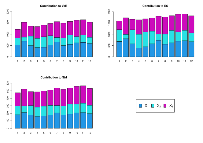
Figure 1: Contributions of $X_{j}$, $j\in\{1,2,3\}$ to the $\text{VaR}_{0.95}$ (top-left), to the $\text{ES}_{0.95}$ (top-right), and to the standard deviation of $S$ (bottom-left), based on Euler’s rule.

The geometrical structure of GFGM copulas inherited from the geometrical structure of multivariate Bernoulli distributions has proven to be a powerful tool for studying the properties of random vectors with GFGM dependence.

The last Example 7 finds the bounds by enumeration of their values in the extremal points, which becomes computationally challenging in high dimensions. Under the assumption of identically distributed risks with GFGM$(p)$ dependence structure, we show the effectiveness of our theoretical results in studying the risk of high dimensional — $d=100$ — portfolios. The extension of these theoretical results to the whole GFGM copulas relies on extending corresponding results in the class of multivariate Bernoulli distributions, and this is part of our ongoing research. Another, more applicative, part is to use this novel geometrical representation to investigate the dependence structure of the class and of their extremal points, which are good candidates for representing extremal dependence also in high dimension.

7 Acknowledgements

This work was partially supported by the Natural Sciences and Engineering Research Council of Canada (Cossette: 04273; Marceau: 05605). This work was also partially supported by the Italian Ministry of Education, University and Research (MIUR), PRIN 2022-PNRR project P2022XT8C8. H. Cossette and E. Marceau would like to thank Dipartimento di Scienze Matematiche ”G. L. Lagrange” (DISMA), Politecnico di Torino, for their wonderful stay during which most of the paper was written.

References

• [4ti2 team, 2018] 4ti2 team (2018). 4ti2—a software package for algebraic, geometric and combinatorial problems on linear spaces. Available at https://4ti2.github.io.
• [Bernard et al., 2014] Bernard, C., Jiang, X., and Wang, R. (2014). Risk aggregation with dependence uncertainty. Insurance: Mathematics and Economics, 54:93–108.
• [Bernard et al., 2017] Bernard, C., Rüschendorf, L., Vanduffel, S., and Yao, J. (2017). How robust is the value-at-risk of credit risk portfolios? The European Journal of Finance, 23(6):507–534.
• [Blier-Wong et al., 2024a] Blier-Wong, C., Cossette, H., Legros, S., and Marceau, E. (2024a). A new method to construct high-dimensional copulas with Bernoulli and Coxian-2 distributions. Journal of Multivariate Analysis, 201:105261.
• [Blier-Wong et al., 2022a] Blier-Wong, C., Cossette, H., and Marceau, E. (2022a). Generating function method for the efficient computation of expected allocations. arXiv preprint arXiv:2207.02654.
• [Blier-Wong et al., 2022b] Blier-Wong, C., Cossette, H., and Marceau, E. (2022b). Stochastic representation of FGM copulas using multivariate Bernoulli random variables. Computational Statistics & Data Analysis, 173:107506.
• [Blier-Wong et al., 2023] Blier-Wong, C., Cossette, H., and Marceau, E. (2023). Risk aggregation with FGM copulas. Insurance: Mathematics and Economics, 111:102–120.
• [Blier-Wong et al., 2024b] Blier-Wong, C., Cossette, H., and Marceau, E. (2024b). Exchangeable FGM copulas. Advances in Applied Probability, 56(1):205–234.
• [Cooley and Tukey, 1965] Cooley, J. W. and Tukey, J. W. (1965). An algorithm for the machine calculation of complex Fourier series. Mathematics of Computation, 19(90):297–301.
• [Cormen et al., 2009] Cormen, T. H., Leiserson, C. E., Rivest, R. L., and Stein, C. (2009). Introduction to Algorithms. MIT Press.
• [Cossette et al., 2013] Cossette, H., Côté, M.-P., Marceau, E., and Moutanabbir, K. (2013). Multivariate distribution defined with Farlie–Gumbel–Morgenstern copula and mixed Erlang marginals: Aggregation and capital allocation. Insurance: Mathematics and Economics, 52(3):560–572.
• [De Berg et al., 1997] De Berg, M., Van Kreveld, M., Overmars, M., and Schwarzkopf, O. (1997). Computational geometry. Springer.
• [Durante and Sempi, 2015] Durante, F. and Sempi, C. (2015). Principles of copula theory. CRC press.
• [Embrechts et al., 1993] Embrechts, P., Grübel, R., and Pitts, S. M. (1993). Some applications of the fast Fourier transform algorithm in insurance mathematics This paper is dedicated to Professor W. S. Jewell on the occasion of his 60th birthday. Statistica Neerlandica, 47(1):59–75.
• [Fontana et al., 2021] Fontana, R., Luciano, E., and Semeraro, P. (2021). Model risk in credit risk. Mathematical Finance, 31(1):176–202.
• [Fontana and Semeraro, 2018] Fontana, R. and Semeraro, P. (2018). Representation of multivariate Bernoulli distributions with a given set of specified moments. Journal of Multivariate Analysis, 168:290–303.
• [Fontana and Semeraro, 2023] Fontana, R. and Semeraro, P. (2023). Exchangeable Bernoulli distributions: High dimensional simulation, estimation, and testing. Journal of Statistical Planning and Inference, 225:52–70.
• [Fontana and Semeraro, 2024] Fontana, R. and Semeraro, P. (2024). High dimensional Bernoulli distributions: Algebraic representation and applications. Bernoulli, 30(1):825–850.
• [Frostig, 2001] Frostig, E. (2001). Comparison of portfolios which depend on multivariate Bernoulli random variables with fixed marginals. Insurance: Mathematics and Economics, 29(3):319–331.
• [Hu and Wu, 1999] Hu, T. and Wu, Z. (1999). On dependence of risks and stop-loss premiums. Insurance: Mathematics and Economics, 24(3):323–332.
• [Müller and Stoyan, 2002] Müller, A. and Stoyan, D. (2002). Comparison Methods for Stochastic Models and Risks. John Wiley.
• [Puccetti and Wang, 2015] Puccetti, G. and Wang, R. (2015). Extremal dependence concepts. Statistical Science, 30(4):485–517.
• [Shaked and Shanthikumar, 2007] Shaked, M. and Shanthikumar, J. G. (2007). Stochastic orders. Springer.
• [Tasche, 1999] Tasche, D. (1999). Risk contributions and performance measurement. Report of the Lehrstuhl für mathematische Statistik, TU München.
• [Willmot and Woo, 2007] Willmot, G. E. and Woo, J.-K. (2007). On the class of Erlang mixtures with risk theoretic applications. North American Actuarial Journal, 11(2):99–115.