Fast Last-Iterate Convergence of Learning in Games Requires Forgetful Algorithms

Abstract

Self-play via online learning is one of the premier ways to solve large-scale two-player zero-sum games, both in theory and practice. Particularly popular algorithms include optimistic multiplicative weights update (OMWU) and optimistic gradient-descent-ascent (OGDA). While both algorithms enjoy $O(1/T)$ ergodic convergence to Nash equilibrium in two-player zero-sum games, OMWU offers several advantages including logarithmic dependence on the size of the payoff matrix and $\tilde{O}(1/T)$ convergence to coarse correlated equilibria even in general-sum games. However, in terms of last-iterate convergence in two-player zero-sum games, an increasingly popular topic in this area, OGDA guarantees that the duality gap shrinks at a rate of $(1/\sqrt{T})$, while the best existing last-iterate convergence for OMWU depends on some game-dependent constant that could be arbitrarily large. This begs the question: is this potentially slow last-iterate convergence an inherent disadvantage of OMWU, or is the current analysis too loose? Somewhat surprisingly, we show that the former is true. More generally, we prove that a broad class of algorithms that do not forget the past quickly all suffer the same issue: for any arbitrarily small $\delta>0$, there exists a $2\times 2$ matrix game such that the algorithm admits a constant duality gap even after $1/\delta$ rounds. This class of algorithms includes OMWU and other standard optimistic follow-the-regularized-leader algorithms.

1 Introduction

Self-play via online learning is one of the premier ways to solve large-scale two-player zero-sum games. Major examples include super-human AIs for Go, Poker (Brown and Sandholm, 2018), and Stratego (Perolat et al., 2022) and alignment of large language models (Munos et al., 2023). In particular, Optimistic Multiplicative Weights Update (OMWU) and Optimistic Gradient Descent-Ascent (OGDA) are two of the most well-known online learning algorithms. When applied to learning a two-player zero-sum game via self-play for $T$ rounds, the average iterates of both algorithms are known to be an $O(1/T)$-approximate Nash equilibrium (Rakhlin and Sridharan, 2013; Syrgkanis et al., 2015), while other algorithms, such as vanilla Multiplicative Weights Update (MWU) and vanilla Gradient Descent-Ascent (GDA), have a slower ergodic convergence rate of $O(1/\sqrt{T})$.

For multiple practical reasons, there is growing interest in studying the last-iterate convergence of these learning dynamics (Daskalakis and Panageas, 2019; Golowich et al., 2020b; Wei et al., 2021; Lee et al., 2021). In this regard, existing results seemingly exhibit a gap between OGDA and OMWU — the duality gap of the last iterate of OGDA is known to decrease at a rate of $O(1/\sqrt{T})$ (Cai et al., 2022; Gorbunov et al., 2022), with no dependence on constants beyond the dimension and the smoothness of the players’ utility functions of the game. In contrast, the existing convergence rate for OMWU depends on some game-dependent constant that could be arbitrarily large, even after fixing the dimension and the smoothness constant of the game (Wei et al., 2021). Given the fundamental role of OMWU in online learning and its other advantages over OGDA (such as its logarithmic dependence on the number of actions), it is natural to ask the following question:

Is the potentially slow last-iterate convergence an inherent disadvantage of OMWU? (*)

Results.

In this work, we show that the answer to this question is yes, contrary to a common belief that better analysis and better last-iterate convergence results similar to those of OGDA are possible for OMWU. More specifically, we show the following.

Theorem (Informal).

For OMWU with constant step size, there is no function $f$ such that the corresponding learning dynamics $\{(x^{t},y^{t})\}_{t\geq 1}$ in two-player zero-sum games has a last-iterate convergence rate of $f(d_{1},d_{2},T)$, where entries of the loss matrix are in $[0,1]$, and $d_{1}$ and $d_{2}$ are the number of actions. More specifically, no function $f$ can satisfy

• $\operatorname{DualityGap}(x^{T},y^{T})\leq f(d_{1},d_{2},T)$ for all $T$.

• $\lim_{T\rightarrow\infty}f(d_{1},d_{2},T)\rightarrow 0$.

Our findings show that, despite the significantly superior regret properties of OMWU compared to OGDA, its last-iterate convergence properties are remarkably worse. In turn, this counters the viewpoint that “Follow-the-Regularized-Leader (FTRL) is better than Online Mirror Descent (OMD)” (van Erven, 2021): crucially, while OMWU is an instance of (optimistic) FTRL, OGDA is an instance of optimistic OMD that cannot be expressed in the FTRL formalism.

We further show that similar negative results extend to several other standard online learning algorithms, including a close variant of OGDA. More concretely, our main results are as follows.

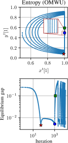
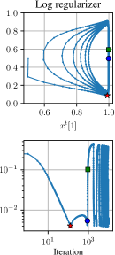
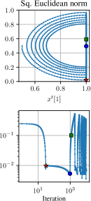
Figure 1: Comparison of the dynamics produced by three variants of OFTRL with different regularizers (negative entropy, logarithmic regularizer, and squared Euclidean norm) and OGDA in the same game $A_{\delta}$ defined in (2) for $\delta:=10^{-2}$. The bottom row shows the duality gap achieved by the last iterates. The OFTRL variants exhibit poor performance due to their lack of forgetfulness, while OGDA converges quickly to the Nash equilibrium. Since the regularizers in the first two plots are Legendre, the dynamics are equivalent to the ones produced by optimistic OMD with the respective Bregman divergences. In the plot for OMWU we observe that $x^{t}[1]$ can get extremely close to the boundary (e.g., in the range $1-e^{-50}<x^{t}[1]<1$). To correctly simulate the dynamics, we used 1000 digits of precision. The red star, blue dot, and green square illustrate the key times $T_{1}$, $T_{2}$, $T_{3}$ defined in our analysis in Section 3.

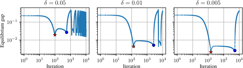
Figure 2: Performance of OMWU on the game $A_{\delta}$ defined in eq. 2 for three choices of $\delta$. In all plots, the learning rate was set to $\eta=0.1$. As predicted by our analysis, the length of the “flat region” between iteration $T_{1}$ (red star) and $T_{2}$ (blue dot) scales inversely proportionally with $\delta$.

• We identify a broad family of Optimistic FTRL (OFTRL) algorithms that do not forget about the past quickly. We prove that, for any sufficiently small $\delta>0$, there exists a $2\times 2$ two-player zero-sum game such that, even after $1/\delta$ iterations, the duality gap of the iterate output by these algorithms is still a constant (Theorem 1). This excludes the possibility of showing a game-independent last-iterate convergence rate similar to that of OGDA.

• We prove that many standard online learning algorithms, such as OFTRL with the entropy regularizer (equivalently, OMWU), the Tsallis entropy family of regularizers, the log regularizer, and the squared Euclidean norm regularizer, all fall into this family of non-forgetful algorithms and thus all suffer from the same slow convergence. Also note that Optimistic OMD (OOMD), another well-known family of algorithms, is equivalent to OFTRL when given a Legendre regularizer. Therefore, OOMD with the entropy, Tsallis entropy, and log regularizer also suffer the same issue.

• Finally, we also generalize our negative results from $2\times 2$ games to $2n\times 2n$ games for any positive integer $n$, strengthening our message that forgetfulness is generally needed in order to achieve fast last-iterate convergence.

Main ideas.

Intuitively, we trace the poor last-iterate convergence properties of OFTRL to its lack of forgetfulness. The high-level idea of our hard $2\times 2$ game instance, parametrized by $\delta>0$, is as follows. First, it has a unique Nash equilibrium at which one player is $O(\delta)$ close to the boundary of the simplex. We refer to the first row of plots in Figure 1, where the equilibrium is noted by a blue dot (note that we can plot only $x[1],y[1]$ for each player, since $x[2]=1-x[1]$ and $y[2]=1-y[2]$). As can be seen, the iterates of OGDA and all three OFTRL variants initially have a two-phase structure. In the first phase, they converge to the lower-right area denoted by a red star in Figure 1. Then, from there all algorithms start moving towards the equilibrium. However, once they enter the vicinity of the equilibrium, the behavior depends on the algorithms. For OGDA, the dynamics start spiraling closer and closer to the equilibrium. On the other hand, for the OFTRL algorithms, the $y$ player has built up a lot of momentum in the direction of increasing $y[1]$, and for this reason they cannot “stop” near the equilibrium. Instead, they start to move away from the equilibrium, and enter a new cycle where they move out towards the starting point of the learning process. This cycle repeats in smaller and smaller semi-ellipses that slowly converge to equilibrium. Note that the semi-ellipses correspond to the seesaw pattern in the equilibrium gap (second row of plots). OFTRL overshoots the equilibrium as it has built up a lot of "memory" of $y[1]$ being better than $y[2]$ along the phase from the red star to the blue circle, and it requires many iterations to "forget" this fact. We show that as we make $\delta$, the parameter defining the nearness to the boundary, smaller and smaller, it takes longer and longer for these semi-ellipses to get close to the equilibrium along the entire path, as illustrated in Figure 2.

Our results are related to numerical observations made in the literature on solving large-scale extensive-form games. There, algorithms based on the regret-matching⁺ (RM⁺) algorithm (Tammelin et al., 2015), combined the counterfactual regret minimization (Zinkevich et al., 2007), perform by far the best in practice. In contrast, the classical regret matching algorithm (Hart and Mas-Colell, 2000) performs much worse, in spite of similar regret guarantees. It was later discovered that RM⁺ corresponds to OGD, while RM corresponds to FTRL (Farina et al., 2021; Flaspohler et al., 2021). It was hypothesized that RM builds up too much negative regret at times, and thus is slow to adapt to changes in the learning dynamics related to the strategy of the other player. These numerical results, and the hypothesis, are consistent with our theoretical findings: FTRL (and thus RM) is not able to “forget,” whereas OGD and OGDA can forget, and thereby quickly adapt to changes in which actions should be played.

1.1 Related Work

The literature on last-iterate convergence of online learning methods in games is vast. In this section, we will cover key contributions focusing on the case of interest for this paper: discrete-time dynamics for two-player zero-sum normal-form games.

Convergence of OGDA. Average-iterate convergence of OGDA has been studied for minimax optimization problems in both the unconstrained (Mokhtari et al., 2020) and constrained settings (Hsieh et al., 2019). Last-iterate convergence of OGDA in unconstrained saddle-point problems has been shown in (Daskalakis et al., 2018; Golowich et al., 2020a). In the (constrained) game setting, Wei et al. (2021); Anagnostides et al. (2022) showed best-iterate convergence to the set of Nash equilibria in any two-player zero-sum game with payoff matrix $A$ at a rate of $O(\textrm{poly}(d_{1},d_{2},\max_{i,j}|A_{i,j}|)/\sqrt{T})$ using constant learning rate, where $d_{1}$ and $d_{2}$ are the number of actions of the players. A stronger result was shown by Cai et al. (2022), who showed that the same rate applies to the last iterate.

Convergence of OMWU. Optimistic multiplicative weights update (also known as optimistic hedge) is often regarded as the premier algorithm for learning in games. Unlike OGDA, it guarantees sublinear regret with a logarithmic dependence on the number of actions, and it is known to guarantee only polylogarithmic regret per player when used in self play even for general-sum games (Daskalakis et al., 2021). It can be applied with similar strong properties beyond normal-form games in several important combinatorial settings (Takimoto and Warmuth, 2003; Koolen et al., 2010; Farina et al., 2022). The work by Daskalakis and Panageas (2019) established asymptotic last-iterate convergence for OMWU in games using a small learning rate under the assumption of a unique Nash equilibrium. Similar asymptotic results without the unique equilibrium assumption were also given by Mertikopoulos et al. (2019); Hsieh et al. (2021). Wei et al. (2021) were the first to provide nonasymptotic learning rates for OMWU. Specifically, they showed a linear rate of convergence in games with a unique equilibrium, albeit with a dependence on a condition number-like quantity that could be arbitrarily large given fixed $d_{1}$, $d_{2}$, and $\max_{i,j}|A_{i,j}|$.This result was later extended by Lee et al. (2021) to extensive-form games. Unlike OGDA, no last-iterate convergence result for OMWU with a polynomial dependence on only the natural parameters of the game (i.e., $d_{1}$, $d_{2}$, and $\max_{i,j}|A_{i,j}|$) is known. As we show in this paper, perhaps surprisingly, this is no coincidence: in general, OMWU does not exhibit a last-iterate convergence rate that solely depends on these parameters, whether polynomial or not.

FTRL vs. OMD. While the last-iterate convergence of instantiations of Optimistic Online Mirror Descent has been observed before, the properties of Follow-the-Regularized-Leader dynamics remain mostly elusive. The present paper partly explains this vacuum: all standard instantiations of optimistic FTRL cannot hope to converge in iterates with only a polynomial dependence on the natural parameters of the game, unlike optimistic OMD. Complications in obtaining last-iterate convergence results for continuous-time FTRL instantiations were already reported by Vlatakis-Gkaragkounis et al. (2020), who showed the necessity of strict Nash equilibria.

Exploiting a no-regret learner. The forgetfulness property that we identify is closely related to the concept of mean-based learning algorithms from Braverman et al. (2018). Intuitively, mean-based algorithms are ones such that if the mean reward for action $a$ is significantly greater than the mean reward for action $b$, then the algorithm selects $b$ with negligible probability. They show that MWU is mean-based, along with Follow-the-Perturbed-Leader and the Exp3 bandit algorithm. Braverman et al. (2018) shows that "mean-based" algorithms are exploitable when learning to bid in first-price auctions, whereas Kumar et al. (2024) shows that OGD does not suffer from this exploitability issue.

2 Preliminaries and Problem Setup

We consider the standard setting of no-regret learning in a zero-sum game $A\in[0,1]^{d_{1}\times d_{2}}$. In each iteration $t\geq 1$, the $x$-player chooses $x^{t}\in\mathcal{X}:=\Delta^{d_{1}}$ while the $y$-player chooses $y^{t}\in\mathcal{Y}:=\Delta^{d_{2}}$. Then the $x$-player receives loss vector $\ell^{t}_{x}=Ay^{t}$ while the $y$-player receives loss vector $\ell^{t}_{y}=-A^{\top}x^{t}$. The goal is to find or approximate a Nash equilibrium $(x^{*},y^{*})$ to the game such that $x^{*}\in\operatorname*{argmin}_{x\in\mathcal{X}}\max_{y\in\mathcal{Y}}x^{\top}Ay$ and $y^{*}\in\operatorname*{argmax}_{y\in\mathcal{Y}}\min_{x\in\mathcal{X}}x^{\top}Ay$. The approximation error of a strategy pair $(x,y)$ is measured by its duality gap, defined as $\operatorname{DualityGap}(x,y)=\max_{y^{\prime}\in\mathcal{Y}}x^{\top}Ay^{\prime}-\min_{x^{\prime}\in\mathcal{X}}{x^{\prime}}^{\top}Ay$, which is always non-negative.

Popular no-regret algorithms for solving the game include the Optimistic Follow-the-Regularized-Leader (OFTRL) algorithm and the Optimistic Online Mirror Descent (OOMD) algorithm, both defined in terms of a certain regularizer $R:\Delta^{d}\rightarrow\mathbb{R}$ (for some general dimension $d$). The corresponding Bregman divergence of $R$ is $D_{R}(x,x^{\prime})=R(x)-R(x^{\prime})-{\mathchoice{\left\langle\nabla R(x^{\prime}),x-x^{\prime}\right\rangle}{\langle\nabla R(x^{\prime}),x-x^{\prime}\rangle}{\langle\nabla R(x^{\prime}),x-x^{\prime}\rangle}{\langle\nabla R(x^{\prime}),x-x^{\prime}\rangle}}$, and the regularizer is $1$-strongly convex if $D_{R}(x,x^{\prime})\geq\frac{1}{2}{\mathchoice{\left\|x-x^{\prime}\right\|}{\|x-x^{\prime}\|}{\|x-x^{\prime}\|}{\|x-x^{\prime}\|}}_{2}^{2}$ for all $x,x^{\prime}\in\Delta^{d}$.

Optimistic Online Mirror Descent (OOMD)

Starting from an initial point $(x^{1},y^{1})=(\widehat{x}^{1},\widehat{y}^{1})$, the OOMD algorithm with regularizer $R$ and steps size $\eta>0$ updates in each iteration $t\geq 2$,

$$\widehat{x}^{t} =\operatorname*{argmin}_{x\in\mathcal{X}}\{\eta{\mathchoice{\left\langle x,\ell^{t-1}_{x}\right\rangle}{\langle x,\ell^{t-1}_{x}\rangle}{\langle x,\ell^{t-1}_{x}\rangle}{\langle x,\ell^{t-1}_{x}\rangle}}+D_{R}(x,\widehat{x}^{t-1})\},\quad x^{t}=\operatorname*{argmin}_{x\in\mathcal{X}}\{\eta{\mathchoice{\left\langle x,\ell^{t-1}_{x}\right\rangle}{\langle x,\ell^{t-1}_{x}\rangle}{\langle x,\ell^{t-1}_{x}\rangle}{\langle x,\ell^{t-1}_{x}\rangle}}+D_{R}(x,\widehat{x}^{t})\},$$ (OOMD)

$$\widehat{y}^{t} =\operatorname*{argmin}_{y\in\mathcal{Y}}\{\eta{\mathchoice{\left\langle y,\ell^{t-1}_{y}\right\rangle}{\langle y,\ell^{t-1}_{y}\rangle}{\langle y,\ell^{t-1}_{y}\rangle}{\langle y,\ell^{t-1}_{y}\rangle}}+D_{R}(y,\widehat{y}^{t-1})\},\quad y^{t}=\operatorname*{argmin}_{y\in\mathcal{Y}}\{\eta{\mathchoice{\left\langle y,\ell^{t-1}_{y}\right\rangle}{\langle y,\ell^{t-1}_{y}\rangle}{\langle y,\ell^{t-1}_{y}\rangle}{\langle y,\ell^{t-1}_{y}\rangle}}+D_{R}(y,\widehat{y}^{t})\}.$$

In particular, we call OOMD with a squared Euclidean norm regularizer, that is, $R(x)=\frac{1}{2}\sum_{i=1}^{d}x[i]^{2}$ optimistic gradient-descent-ascent (OGDA). When $R$ is the negative entropy, that is, $R(x)=\sum_{i=1}^{d}x[i]\log x[i]$, we call the resulting OOMD algorithm optimistic multiplicative weights update (OMWU). OGDA and OMWU have been extensively studied in the literature regarding their last-iterate convergence properties in zero-sum games. Specifically, both OMWU and OGDA guarantee that $(x^{t},y^{t})$ approaches to a Nash equilibrium as $t\to\infty.$

Optimistic Follow-the-Regularized-Leader (OFTRL)

Define the cumulative loss vectors $L^{t}_{x}:=\sum_{k=1}^{t}\ell^{k}_{x}$ and $L^{t}_{y}:=\sum_{k=1}^{t}\ell^{k}_{y}$. The update rule of OFTRL with regularizer $R$ is for each $t\geq 1$,

$$x^{t} =\operatorname*{argmin}_{x\in\mathcal{X}}\left\{{\mathchoice{\left\langle x,L^{t-1}_{x}+\ell^{t-1}_{x}\right\rangle}{\langle x,L^{t-1}_{x}+\ell^{t-1}_{x}\rangle}{\langle x,L^{t-1}_{x}+\ell^{t-1}_{x}\rangle}{\langle x,L^{t-1}_{x}+\ell^{t-1}_{x}\rangle}}+\frac{1}{\eta}R(x)\right\},$$ (OFTRL)

$$y^{t} =\operatorname*{argmin}_{y\in\mathcal{Y}}\left\{{\mathchoice{\left\langle y,L^{t-1}_{y}+\ell^{t-1}_{y}\right\rangle}{\langle y,L^{t-1}_{y}+\ell^{t-1}_{y}\rangle}{\langle y,L^{t-1}_{y}+\ell^{t-1}_{y}\rangle}{\langle y,L^{t-1}_{y}+\ell^{t-1}_{y}\rangle}}+\frac{1}{\eta}R(y)\right\}.$$

Throughout the paper, we consider the following regularizers:

• Negative entropy ($R(x)=\sum_{i=1}^{d}x[i]\log x[i]$): the resulting OFTRL algorithm coincides with OMWU defined by the OOMD framework previously.

• Squared Euclidean norm ($R(x)=\frac{1}{2}\sum_{i=1}^{d}x[i]^{2}$): note that the resulting algorithm is different from OGDA since the squared Euclidean norm is not a Legendre regularizer. As we will show, the two algorithms behave very differently in terms of last-iterate convergence.

• Log barrier ($R(x)=\sum_{i=1}^{d}-\log(x[i])$): we also call it the log regularizer.

• Negative Tsallis entropy regularizers ($R(x)=\frac{1-\sum_{i=1}^{d}(x[i])^{\beta}}{1-\beta}$ parameterized by $\beta\in(0,1)$).

The 2-dimension case

We denote $x\in\mathbbm{R}^{2}$ as $x=[x[1],x[2]]^{\top}$. For $d_{1}=2$, finding $x^{t}$ of OFTRL reduces to the following 1-dimensional optimization problem:

$$x^{t}[1]=\operatorname*{argmin}_{x\in[0,1]}\left\{x\cdot(L^{t-1}_{x}[1]+\ell^{t-1}_{x}[1]-L^{t-1}_{x}[2]-\ell^{t-1}_{x}[2])+\frac{1}{\eta}R(x)\right\},\quad x^{t}[2]=1-x^{t}[1],$$

where we slightly abuse the notation and denote $R(x)=R([x,1-x])$ for $x\in[0,1]$. We introduce two notations (the case for the $y$-player is similar): let $e^{t}_{x}=\ell^{t}_{x}[1]-\ell^{t}_{x}[2]$ be the difference between the losses of the two actions, and $E^{t}_{x}=\sum_{k=1}^{t}e^{k}_{x}$ be the cumulative difference between the losses of the two actions. For OFTRL, it is clear that the update of $x^{t}$ only depends on the differences $E^{t-1}_{x},e^{t-1}_{x}$, the step size $\eta$, and the regularizer $R$. For this reason, we define $F_{\eta,R}:\mathbb{R}\rightarrow[0,1]$ as follows:

$$F_{\eta,R}(e):=\operatorname*{argmin}_{x\in[0,1]}\left\{x\cdot e+\frac{1}{\eta}R(x)\right\}.$$ (1)

We assume the function $F_{\eta,R}$ is well-defined, i.e., the above optimization problem admits a unique solution in $[0,1]$. This is a condition easily satisfied, for example, when the regularizer $R$ is strongly convex. Then the OFTRL algorithm can be written as

$$x^{t}[1]=F_{\eta,R}(E^{t-1}_{x}+e^{t-1}_{x}),\quad x^{t}[2]=1-x^{t}[1].$$

The following lemma shows that the function $F_{\eta,R}$ is non-increasing (we defer missing proofs in the section to Appendix A).

Lemma 1 (Monotonicity of $F_{\eta,R}$).

The function $F_{\eta,R}(\cdot):\mathbb{R}\rightarrow[0,1]$ defined in (1) is non-increasing.

We present some blanket assumptions on the regularizer, which are satisfied by all the regularizers introduced before.

Assumption 1.

We assume that the regularizer $R$ satisfies the following properties: the function $F_{\eta,R}:\mathbb{R}\rightarrow[0,1]$ defined in (1) is,

• Unbiased: $F_{\eta,R}(0)=\frac{1}{2}$.

• Rational: $\lim_{E\rightarrow-\infty}F_{\eta,R}(E)=1$ and $\lim_{E\rightarrow+\infty}F_{\eta,R}(E)=0$.

• Lipschitz continuous: There exists $L\geq 0$ such that $F_{1,R}$ is $L$-Lipschitz.

Item 1 in 1 shows that the initial strategy is the uniform distribution over the two actions, which is standard in practice. The rational assumption (item 2 in 1) is natural since otherwise, the algorithm could not even converge to a pure Nash equilibrium. The Lipschitzness (item 3 in 1) is implied when the regularizer is strongly convex over $[0,1]^{2}$ (see Lemma 4), and it further implies Lipschitzness of $F_{\eta,R}$ for any $\eta$ as shown in the following proposition.

Proposition 1.

The function $F_{\eta,R}$ satisfies $F_{\eta,R}{\mathchoice{\left(E/\eta\right)}{(E/\eta)}{(E/\eta)}{(E/\eta)}}=F_{1,R}(E)$. If $F_{1,R}$ is $L$-Lipschitz, then $F_{\eta,R}$ is $\eta L$-Lipschitz for any $\eta>0$.

3 Slow Convergence of OFTRL: A Hard Game Instance

We give negative results on the last-iterate convergence properties of OFTRL by studying its behavior on a surprisingly simple $2\times 2$ two-player zero-sum games. The game’s loss matrix $A_{\delta}$ is parameterized by $\delta\in(0,\frac{1}{2})$ and is defined as follows:

$$A_{\delta}\coloneqq\begin{bmatrix}\frac{1}{2}+\delta&\frac{1}{2}\\[5.69054pt] 0&1\end{bmatrix}.$$ (2)

3.1 Basic Properties

We summarize some useful properties of $A_{\delta}$ in the following proposition (missing proofs of this section can be found in Appendix B).

Proposition 2.

The matrix game $A_{\delta}$ satisfies:

• $A_{\delta}$ has a unique Nash equilibrium $x^{*}=[\frac{1}{1+\delta},\frac{\delta}{1+\delta}]$ and $y^{*}=[\frac{1}{2(1+\delta)},\frac{1+2\delta}{2(1+\delta)}]$.

• For a strategy pair $(x^{t},y^{t})$, the loss vectors (i.e., gradients) for the two palyers are respctively:

  $$\ell^{t}_{x}=A_{\delta}y^{t}=\begin{bmatrix}\frac{1}{2}+\delta y^{t}[1]\\ 1-y^{t}[1]\end{bmatrix}\quad\ell^{t}_{y}=-A_{\delta}^{\top}x^{t}=-\begin{bmatrix}(\frac{1}{2}+\delta)x^{t}[1]\\ 1-\frac{1}{2}x^{t}[1]\end{bmatrix}.$$ (3)

  Moreover,

  $$e^{t}_{x}=\ell^{t}_{x}[1]-\ell^{t}_{x}[2]=-\frac{1}{2}+(1+\delta)y^{t}[1]\in[-\frac{1}{2},\frac{1}{2}+\delta]$$

  $$e^{t}_{y}=\ell^{t}_{y}[1]-\ell^{t}_{y}[2]=1-(1+\delta)x^{t}[1]\in[-\delta,1].$$

In particular, we notice that $e^{t}_{y}\geq-\delta$. It implies that if the cumulative differences between the losses of the two actions $E^{t}_{y}$ is large, then it takes $\Omega(\frac{1}{\delta})$ iterations to make $E^{t}_{y}$ small (close to $0$). This has important implications for non-forgetful algorithms like OFTRL that look at the whole history of losses. Since OFTRL chooses the strategy $y^{t}$ based on $E^{t}_{y}$, it could be trapped in a bad action for a long time even if the current gradients suggest that the other action is better. This is the key observation for our main negative results on the slow last-iterate convergence rates of OFTRL.

The following lemma shows that in a particular region of $(x,y)$, the duality gap is a constant.

Lemma 2.

Let $\delta,\epsilon\in(0,\frac{1}{2})$. For any $x,y\in\Delta^{2}$ such that $x[1]\geq\frac{1}{1+\delta}$ and $y[1]\geq\frac{1}{2}+\epsilon$, the duality gap of $(x,y)$ for game $A_{\delta}$ (defined in (2)) satisfies $\operatorname{DualityGap}(x,y)\geq\epsilon.$

3.2 Slow Last-Iterate Convergence

We further require the following assumption on the regularizer $R$ (and thus the function $F_{1,R}$).

Assumption 2.

Let $L$ be the Lipschitness constant of $F_{1,R}$ in 1. Denote constant $c_{1}=\frac{1}{2}-F_{1,R}(\frac{1}{20L})$. There exist universal constants $\delta^{\prime},c_{2}>0$ and $c_{3}\in(0,\frac{1}{2}]$ such that for any $0<\delta\leq\delta^{\prime}$,

• If $F_{1,R}(E)\geq\frac{1}{1+\delta}$, then $F_{1,R}(-\frac{c_{1}^{2}}{30L\delta}+E)\geq\frac{1+c_{3}}{1+c_{3}+\delta}$

• If $F_{1,R}(E)\geq\frac{1}{2(1+\delta)}$, then $F_{1,R}(-\frac{c_{3}c_{1}^{2}}{120L}+\frac{\delta}{4L}+E)\geq\frac{1}{2}+c_{2}$.

Although 2 is technical, the idea is simple. Item 1 in 2 states that if a loss difference $E<0$ already makes $F_{1,R}(E)\geq\frac{1}{1+\delta}$, then the loss difference $E^{\prime}=E-\Omega(\frac{1}{\delta})$ is able to make $F_{1,R}(E^{\prime})$ greater than $F_{1,R}(E)$ by a margin of $\Omega(\delta)$. Item 2 in 2 states that if a loss difference $E$ already makes $F_{1,R}(E)\geq\frac{1}{2(1+\delta)}\approx\frac{1}{2}$, then the loss difference $E^{\prime}=E-\Omega(1)$ is able to make $F_{1,R}(E^{\prime})$ greater than $\frac{1}{2}$ by a constant margin $c_{2}$. In Appendix C, we verify that 2 holds for the negative entropy, squared Euclidean norm, the log barrier, and the negative Tsallis entropy regularizers.

Now we present the main result of the section showing that even after $\Omega(1/\delta)$ iterations, the duality gap of the iterate output by OFTRL is still a constant.

Theorem 1.

Assume the regularizer $R$ satisfies 1 and 2. For any $\delta\in(0,\hat{\delta})$, where $\hat{\delta}$ is a constant depending only on the constants $c_{1}$ and $\delta^{\prime}$ defined in 2, the OFTRL dynamics on $A_{\delta}$ (defined in (2)) with any step size $\eta\leq\frac{1}{4L}$ satisfies the following: there exists an iteration $t\geq\frac{c_{1}}{3\eta L\delta}$ with a duality gap of at least $c_{2}$, a strictly positive constant defined in 2.

Figure 3: Pictorial depiction of the three stages incurred by the OFTRL dynamics in the game $A_{\delta}$ defined in (2). The point $z^{*}$ denotes the unique Nash equilibrium. The times $T_{1}$ and $T_{2}$ are shown for concrete instantiations of OFTRL in Figure 1 by a red star and a blue dot, respectively. The times $T_{s}$ and $T_{h}$ are defined in the proof of Theorem 1 in Section B.2.

Proof Sketch:

We decompose the analysis into three stages as illustrated in Figure 3. We describe the three stages and the high-level ideas of our proof below and defer the full proof to Section B.2.

• Stage I: Recall that $x^{1}[1]=y^{1}[1]=\frac{1}{2}$ by 1. In Stage I, we show that $x^{t}[1]$ will increase and denote $T_{1}\geq 1$ the first iteration where $x^{t}[1]\geq\frac{1}{1+\delta}$. The existence of $T_{1}$ can be proved by contradiction (1). Since $x^{t}[1]<\frac{1}{1+\delta}$ before the end of Stage I, the loss vector for the $y$-player satisfies $e^{t}_{y}=\ell^{t}_{y}[1]-\ell^{t}_{y}[2]\geq 0$, meaning action $1$ is worse than action $2$. We use this to show that finally $y^{T_{1}}[1]\leq\frac{1}{2}-c_{1}$ with $c_{1}$ defined in 2.

• Stage II: Now that we have $y^{T_{1}}[1]\leq\frac{1}{2}-c_{1}$, we denote $T_{2}>T_{1}$ the first iteration where $y^{T_{2}}[1]\geq\frac{1}{2(1+\delta)}>\frac{1}{2}-c_{1}$. The existence of $T_{2}$ can be proved by contradiction again (2). We remark that in order to increase $y^{t}[1]$, the loss vector must satisfies $e^{t}_{y}<0$. However, the game matrix $A_{\delta}$ guarantees that $e^{t}_{y}\geq-\delta$ no matter what the $x$-player is playing (Proposition 2). Thus by the $\eta L$-Lipschitzness of $F_{\eta,R}$ (Proposition 1), the per-iteration increase in $y^{t}[1]$ is at most $\eta L\delta$. Therefore, we know $T_{2}-T_{1}=\Omega(\frac{c_{1}}{\eta L\delta})$. But during $[T_{1},T_{2}]$, we have $e^{t}_{x}<0$ for the $x$-player which implies its difference $E^{T_{2}}_{x}\leq E^{T_{1}}_{x}-\Omega(\frac{1}{\eta L\delta})$ further grows by at least $\Omega(\frac{1}{\eta L\delta})$. In other words, $x^{t}[1]$ is very close to $1$, and the cumulative loss for action 1 is much smaller than that of action 2.

• Stage III: We start with $y^{T_{2}}[1]\geq\frac{1}{2(1+\delta)}$. Moreover, $y^{t}[1]$ could keep increasing if $x^{t}[1]\geq\frac{1}{1+\delta}$ since that implies $e^{t}_{y}\leq 0$. Now the question is how long would the $x$-player stay close to the boundary, i.e, $x^{t}[1]\geq\frac{1}{1+\delta}$. Since OFTRL-type algorithms are not forgetful, this happens only when $E^{t}_{x}\geq E^{T_{1}}_{x}$ (recall $x^{T_{1}}[1]\geq\frac{1}{1+\delta}$). But we have at the end of stage II, $E^{T_{2}}_{x}\leq E^{T_{1}}_{x}-\Omega(\frac{1}{\eta L\delta})$. Since $e^{t}_{x}\leq 1$, we know $x^{t}[1]\geq\frac{1}{1+\delta}$ even after $\Omega(\frac{1}{\eta L\delta})$ iterations. Define $T_{3}=T_{2}+\Omega(\frac{1}{\eta L\delta})$. During $[T_{2},T_{3}]$, the $y$-player always receives loss such that $e^{t}_{y}\leq 0$ and we prove that in the end $y^{T_{3}}[1]\geq\frac{1}{2}+c_{2}$ for some constant $c_{2}$.

• Conclusion: Finally, we get one iteration $T_{3}\geq\Omega(\frac{1}{\eta L\delta})$ with $x^{T_{3}}[1]\geq\frac{1}{1+\delta}$ and $y^{T_{3}}[1]\geq\frac{1}{2}+c_{2}$. Using Lemma 2, the duality gap of $(x^{T_{3}},y^{T_{3}})$ is at least $c_{2}>0$.

Theorem 1 immediately implies the following (proof deferred to Section B.3).

Theorem 2.

For optimistic FTRL with any regularizer satisfying 1 and 2 and constant steps size $\eta\leq\frac{1}{4L}$ ($L$ is defined in 1), there is no function $f$ such that the corresponding learning dynamics $\{(x^{t},y^{t})\}_{t\geq 1}$ in two-player zero-sum games has a last-iterate convergence rate of $f(d_{1},d_{2},T)$, where entries of the loss matrix are in $[0,1]$, and $d_{1}$ and $d_{2}$ are the number of actions. More specifically, no function $f$ can satisfy

• $\operatorname{DualityGap}(x^{T},y^{T})\leq f(d_{1},d_{2},T)$ for all $T$.

• $\lim_{T\rightarrow\infty}f(d_{1},d_{2},T)\rightarrow 0$.

Theorem 1 and Theorem 2 provide impossibility results for getting a last-iterate convergence rate for OFTRL that solely depends on the bounded parameters, even in two-player zero-sum games. Moreover, they show the necessity of forgetfulness for fast last-iterate convergence in games since OGDA has a last-iterate convergence rate of $O(\frac{\operatorname{poly}(d_{1},d_{2})}{\sqrt{T}})$ (Cai et al., 2022; Gorbunov et al., 2022).

4 Extension to Higher Dimensions

In this section, we extend our negative results from $2\times 2$ matrix games to games with higher dimensions. We start by showing an equivalence result for a single player (say, the first player). We assume that a decision maker is using OFTRL with a 1-strongly convex (w.r.t. the $\ell_{2}$ norm) and separable regularizer $R(x)=R_{1}(x_{1})+R_{2}(x_{2})$ to choose decisions. At a given time time $t$, they see a loss $\ell^{t}\in[0,1]^{2}$.

Now consider the following $2n$-dimensional decision problem: The player uses OFTRL using the regularizer $\hat{R}(\hat{x})=\sum_{i=1}^{n}R_{1}(\hat{x}_{i})+\sum_{i=n+1}^{2n}R_{2}(\hat{x}_{i})$, i.e., they use $R_{1}$ on the first half of actions, and $R_{2}$ on the second half. This is again a 1-strongly convex regularizer (w.r.t. the $\ell_{2}$ norm). Suppose the decision maker sees the rescaled and duplicated version of the losses $\ell^{1},\ldots,\ell^{T}$ from the 2-dimensional case: $\hat{\ell}^{t}_{i}=\frac{1}{n^{\alpha}}\ell^{t}_{1}$ if $i\leq n$, and $\hat{\ell}^{t}_{i}=\frac{1}{n^{\alpha}}\ell^{t}_{2}$ if $i>n$. The parameter $\alpha$ will be chosen later based on the regularizer.

Now we wish to show that by choosing $\alpha$ in the right way, we get that the decisions for the $2$-dimensional and $2n$-dimensional OFTRL algorithms are equivalent. Let $x^{1},\ldots,x^{T}$ be the 2-dimensional OFTRL decisions, and let $\hat{x}^{1},\ldots,\hat{x}^{T}$ be the $2n$-dimensional OFTRL decisions. Then, we want to show that $\sum_{i=1}^{n}\hat{x}_{i}^{t}=x^{t}[1]$ and $\sum_{i=n+1}^{2n}\hat{x}_{i}^{t}=x^{t}[2]$ for all $t$.

Lemma 3.

Let the losses $\hat{\ell}^{1},\ldots,\hat{\ell}^{T}$ satisfy the duplication procedure given in the preceding paragraph. Then for any time $t$, we have $\hat{x}^{t}_{1}=\cdots=\hat{x}^{t}_{n}$ and $\hat{x}^{t}_{n+1}=\cdots=\hat{x}^{t}_{2n}$.

Proof.

Suppose not and let $\hat{x}^{t}$ be the corresponding solution. Then the optimal solution is such that $\hat{x}^{t}_{i}\neq\hat{x}^{t}_{k}$ for some $i,k$ both less than $n$, or both greater than $n$. But then, by symmetry, we have that there is more than one optimal solution to the OFTRL optimization problem at time $t$: the objective is exactly the same if we create a new solution where we swap the values of $\hat{x}^{t}_{i}$ and $\hat{x}^{t}_{k}$. This is a contradiction due to strong convexity. ∎

From lemma 3, we have that the OFTRL decision problem in $2n$ dimensions can equivalently be written as a $2$-dimensional decision problem: Since the first $n$ entries must be the same, we can simply optimize over that one shared value, say $x^{t}[1]$, which we use for all $n$ entries, and similarly we use $x^{t}[2]$ for the second half of the entries. Let $\mathrm{Dupl}:\Delta^{2}\rightarrow\Delta^{2n}$ be a function that maps the two-dimensional solution into the corresponding duplicated $2n$-dimensional solution. The equivalent $2$-dimensional problem is then:

$$\hat{x}^{t} =\mathrm{Dupl}\left[\operatorname*{argmin}_{x\in\frac{1}{n}\cdot\Delta^{2}}\left\{\frac{n}{n^{\alpha}}\left\langle x,\sum_{\tau=1}^{t-1}\ell^{\tau}+\ell^{t-1}\right\rangle+\frac{n}{\eta}R_{1}(x[1])+\frac{n}{\eta}R_{2}(x[2])\right\}\right]$$

$$=\mathrm{Dupl}\left[\frac{1}{n}\cdot\operatorname*{argmin}_{x\in\Delta^{2}}\left\{\frac{n}{n^{\alpha}}\left\langle\frac{1}{n}x,\sum_{\tau=1}^{t-1}\ell^{\tau}+\ell^{t-1}\right\rangle+\frac{n}{\eta}R(x/n)\right\}\right]$$

$$=\mathrm{Dupl}\left[\frac{1}{n}\cdot\operatorname*{argmin}_{x\in\Delta^{2}}\left\{\left\langle x,\sum_{\tau=1}^{t-1}\ell^{\tau}+\ell^{t-1}\right\rangle+\frac{n^{\alpha+1}}{\eta}R(x/n)\right\}\right].$$

Euclidean regularizer: this regularizer is homogeneous of degree two. Choosing $\alpha=1$, the inner minimization problem is exactly the same as the one solved by OFTRL in two dimensions.

Entropy regularizer: we set $\alpha=0$ to get equivalence:

$$nR(x/n)=\sum_{i=1}^{2}x[i]\log(x[i]/n)=\sum_{i=1}^{2}x[i]\log x[i]-\sum_{i=1}^{2}x[i]\log n=\sum_{i=1}^{2}x[i]\log x[i]-\log n.$$

Now we have equivalence because the last term is a constant that does not affect the $\operatorname*{argmin}$.

Log regularizer: we set $\alpha=-1$ to get equivalence, using similar logic as for entropy:

$$R(x/n)=\sum_{i=1}^{2}-\log(x[i]/n)=2\log n+\sum_{i=1}^{2}-\log x[i].$$

Tsallis entropy regularizer: we set $\alpha=-1+\beta$ to get equivalence, using similar logic as for entropy:

$$n^{\beta}R(x/n)=n^{\beta}\cdot\frac{1-\sum_{i=1}^{2}(\frac{x[i]}{n})^{\beta}}{1-\beta}=\frac{n^{\beta}-1}{1-\beta}+\frac{1-\sum_{i=1}^{2}x[i]^{\beta}}{1-\beta}.$$

Putting together the above, we can now construct $2n\times 2n$ loss matrices whose learning dynamics are equivalent to the learning dynamics in our $2\times 2$ games given in the preceding sections. This implies the following theorem.

Theorem 3.

For any loss matrix $A\in[0,1]^{2\times 2}$, there exists a loss matrix $\hat{A}\in[0,n^{-\alpha}]^{2n\times 2n}$ such that for the Euclidean ($\alpha=1$), entropy ($\alpha=0$), Tsallis ($\beta\in(0,1)$ and $\alpha=-1+\beta$), and log ($\alpha=-1$) regularizers, the resulting OFTRL learning dynamics are equivalent in the two games.

Combining Theorem 1 and Theorem 3, we have the following:

Corollary 1.

In the same setup as Theorem 3, under 1 and 2, there exists a game matrix $\hat{A}_{\delta}\in[0,n^{-\alpha}]^{2n\times 2n}$ such that the OFTRL learning dynamics with any step size $\eta\leq\frac{1}{4L}$ satisfies the following: there exists an iteration $t\geq\frac{c_{1}}{3\eta L\delta}$ with a duality gap at least $c_{2}n^{-\alpha}$.

Since $\alpha=0$ for the entropy regularizer, the same results hold more generally for games where one player has more actions than the other. In particular, we can create a $2n\times 2m$ game such that the resulting dynamics are equivalent to those in a $2\times 2$ game. This does not work for the Euclidean and log regularizers because the rescaling factors would be different for the row and column players.

5 Conclusion and Discussions

In this paper, we study last-iterate convergence rates of OFTRL algorithms with various popular regularizers, including the popular OMWU algorithm. Our main results show that even in simple $2\times 2$ two-player zero-sum games parametrized by $\delta>0$, the lack of forgetfulness of OFTRL leads to the duality gap remaining constant even after $1/\delta$ iterations (Theorem 1). As a corollary, we show that the last-iterate convergence rate of OFTRL must depend on a problem-dependent constant that can be arbitrarily bad (Theorem 2). This highlights a stark contrast with OOMD algorithms: while OGDA with constant step size achieves a $O(\frac{1}{\sqrt{T}})$ last-iterate convergence rate, such a guarantee is impossible for OMWU or more generally OFTRL.

We now discuss several interesting questions regarding the convergence guarantees of learning in games and leave them as future directions.

Best-Iterate Convergence Rates

While we focus on the last-iterate (i.e., $\operatorname{DualityGap}(x^{T},y^{T})$), the weaker notion of best-iterate (i.e., $\min_{t\in[T]}\operatorname{DualityGap}(x^{t},y^{t})$) is also of both practical and theoretical interest. By definition, we know the best-iterate convergence rate is at least as good as the last-iterate convergence rate and could be much faster. This raises the following question:

What is the best-iterate convergence rate of OMWU/OFTRL?

To our knowledge, there are no concrete results on the best-iterate convergence rates of OMWU or other OFTRL algorithms. For completeness, we show that for our counterexamples $A_{\delta}$ (defined in (2)), OMWU enjoys a $O(\frac{1}{\ln T})$ best-iterate convergence rate (Appendix D). Although the rate is very slow, it does not depend on $\delta$. It would be interesting to extend our negative results to the best-iterate convergence rates (by finding a different hard game instance) or develop fast best-iterate convergence rates of OMWU/OFTRL.

Dynamic Step Sizes

Our negative results hold for OFTRL with fixed step sizes. We conjecture that the slow last-iterate convergence of OFTRL persists even with dynamic step sizes. In particular, we believe our counterexamples still work for OFTRL with decreasing step sizes. This is because decreasing the step size makes the players move even slower, and they may be trapped in the wrong direction for a longer time due to the lack of forgetfulness. In Appendix E, we include numerical results for OMWU with adaptive stepsize akin to Adagrad (Duchi et al., 2011), which supports our intuition. We observe the same cycling behavior as for fixed step size. While the cycle is smaller compared to that of fixed step sizes, the dynamics take more steps to finish each cycle. Investigating the effect of dynamic step sizes on last-iterate convergence rates is an interesting future direction.

Slow Convergence due to Lack of Forgetfulness

Our work shows that various OFTRL-type algorithms do not have fast last-iterate convergence rates for learning in games. Our proof and hard game instance build on the intuition that these algorithms lack forgetfulness: they do not forget the past quickly. It would be interesting to formalize this intuition further and give a general condition for algorithms under which they suffer slow last-iterate convergence.

Appendix A Missing Proofs in Section 2

A.1 Proof of Lemma 1

Proof.

Let $e_{1}<e_{2}$. Denote $x_{1}=F_{\eta,R}(e_{1})$ and $x_{2}=F_{\eta,R}(e_{2})$. By definition, we have

$$e_{2}(x_{2}-x_{1})\leq\frac{1}{\eta}{\mathchoice{\left(R(x_{1})-R(x_{2})\right)}{(R(x_{1})-R(x_{2}))}{(R(x_{1})-R(x_{2}))}{(R(x_{1})-R(x_{2}))}}\leq e_{1}(x_{2}-x_{1}).$$

Since $e_{1}<e_{2}$, we have $x_{2}\leq x_{1}$. ∎

A.2 Proof of Proposition 1

Proof.

By definition,

$$F_{\eta,R}{\mathchoice{\left(\frac{E}{\eta}\right)}{(\frac{E}{\eta})}{(\frac{E}{\eta})}{(\frac{E}{\eta})}} =\operatorname*{argmin}_{x\in[0,1]}\left\{x\cdot\frac{E}{\eta}+\frac{1}{\eta}R(x)\right\}=\operatorname*{argmin}_{x\in[0,1]}\left\{x\cdot E+R(x)\right\}=F_{1,R}(E).$$

The second claim on the Lipschitzness follows directly. ∎

Appendix B Missing Proofs in Section 3

B.1 Proof of Lemma 2

Proof.

We have

$$\operatorname{DualityGap}(x,y) =\max_{\tilde{y}\in\Delta^{2}}x^{\top}A_{\delta}\tilde{y}-\min_{\tilde{x}\in\Delta^{2}}\tilde{x}^{\top}A_{\delta}y$$

$$=\max_{i\in\{1,2\}}(A_{\delta}^{\top}x)[i]-\min_{i\in\{1,2\}}(Ay_{\delta})[i]$$

$$=(\frac{1}{2}+\delta)x[1]-(1-y[1]) x[1]\geq\frac{1}{1+\delta},\epsilon>0$$ ()

$$\geq\frac{1}{2}\frac{1+2\delta}{1+\delta}-\frac{1}{2}+\epsilon$$

$$\geq\epsilon.$$

∎

B.2 Proof of Theorem 1

Proof.

Recall that $c_{1}=\frac{1}{2}-F_{1,R}(\frac{1}{20L})$ defined in 2. We fix any $\delta<\min\{\frac{1}{15},\frac{c_{1}}{6},\frac{c_{1}^{2}}{300},\delta^{\prime}\}$. Since $\delta<\delta^{\prime}$, 2 holds. We will prove that there exists an iteration $t\geq\frac{c_{1}}{3\eta L\delta}$ with duality gap $c_{2}$.

Proof Plan:

We decompose the analysis into three stages. Below, we describe the three stages and the high-level ideas in our proof.

• Stage I: Recall that $x^{1}[1]=y^{1}[1]=\frac{1}{2}$. In Stage I, we show that $x^{t}[1]$ will increase and denote $T_{1}\geq 1$ the first iteration where $x^{t}[1]\geq\frac{1}{1+\delta}$. The existence of $T_{1}$ can be proved by contradiction (1). Since before the end of Stage I, $x^{t}[1]<\frac{1}{1+\delta}$, the loss vector for the $y$-player satisfies $e^{t}_{y}=\ell^{t}_{y}[1]-\ell^{t}_{y}[2]\geq 0$ meaning action $1$ is worse than action $2$. We will prove that finally $y^{T_{1}}[1]\leq\frac{1}{2}-c_{1}$.

• Stage II: Now we have that $y^{T_{1}}[1]\leq\frac{1}{2}-c_{1}$, we denote $T_{2}>T_{1}$ the first iteration where $y^{T_{2}}[1]\geq\frac{1}{2(1+\delta)}>\frac{1}{2}-c_{1}$. We remark that in order to increase $y^{t}[1]$, the loss vector must satisfy $e^{t}_{y}<0$. However, the game matrix $A_{\delta}$ guarantees that $e^{t}_{y}\geq-\delta$ no matter what the $x$-player is playing. Thus by the $\eta L$-Lipschitzness of $F_{\eta,R}$ (Lemma 4), the increase in $y^{t}[1]$ is at most $\eta L\delta$. Therefore, we know $T_{2}-T_{1}=\Omega(\frac{c_{1}}{\eta L\delta})$. But during $[T_{1},T_{2}]$, for the $x$-player, we have $e^{t}_{x}<0$ which implies its cumulative loss $E^{T_{2}}_{x}\leq E^{T_{1}}_{x}-\Omega(\frac{1}{\eta L\delta})$. In other words, $x^{t}[1]$ is very close to $1$ and the cumulative loss for action 1 is much smaller than that of action 2.

• Stage III: Now we have $y^{T_{2}}[1]\geq\frac{1}{2(1+\delta)}$ and that $y^{t}[1]$ could keep increasing if $x^{t}[1]\geq\frac{1}{1+\delta}$ since then the loss satisfies $e^{t}_{y}\leq 0$. Now the question is how long would the $x$-player stay close to the boundary, i.e, $x^{t}[1]\geq\frac{1}{1+\delta}$. Since OFTRL-type algorithms are not forgetful, this happens only when $E^{t}_{x}\geq E^{T_{1}}_{x}$ (recall $x^{T_{1}}[1]\geq\frac{1}{1+\delta}$). But we have at the end of stage II, $E^{T_{2}}_{x}\leq E^{T_{1}}_{x}-\Omega(\frac{1}{\eta L\delta})$. Since$e^{t}_{x}$ is bounded by a constant, we know $x^{t}[1]\geq\frac{1}{1+\delta}$ even after $\Omega(\frac{1}{\eta L\delta})$ iterations. Define $T_{3}=T_{2}+\Omega(\frac{1}{\eta L\delta})$. During $[T_{2},T_{3}]$, the $y$-player always receives loss such that $e^{t}_{y}\leq 0$ and we prove that $y^{T_{3}}[1]\geq\frac{1}{2}+c_{2}$ for some constant $c_{2}$.

• Conclusion Finally we get one iteration $T_{3}\geq\Omega(\frac{1}{\eta L\delta})$ with $x^{T_{3}}[1]\geq\frac{1}{1+\delta}$ and $y^{T_{3}}[1]\geq\frac{1}{2}+c_{2}$, Using Lemma 2, the duality gap of $(x^{T_{3}},y^{T_{3}})$ is at least $c_{2}$.

Stage I:

We know $x^{1}[1]=y^{1}[1]=\frac{1}{2}$. We define (i) $T_{s}>1$ to be the smallest iteration such that $x^{T_{s}}[1]\geq\frac{3}{4}$ and (ii) $T_{1}>T_{s}$ to be the smallest iteration such that $x^{T_{1}}[1]\geq\frac{1}{1+\delta}$. Both $T_{s}$ and $T_{1}$ must exist, and the reason will become clear in the following analysis. We postpone the proof of this fact in 1 at the end of this paragraph.

Notice from Proposition 2, the difference $e^{t}_{x}$ is lower bounded: $e^{t}_{x}\geq-\frac{1}{2}$ for any $t$. Thus $E^{t-1}_{x}+e^{t-1}_{x}\geq-\frac{t}{2}$ for any $t\geq 1$. Since $x^{T_{s}}[1]\geq\frac{3}{4}>\frac{1}{2}$, we know that $E^{T_{s}-1}_{x}+e^{T_{s}-1}_{x}<0$. As $F_{\eta,R}$ is $\eta L$-Lipschitz,

$$\frac{1}{4}\leq x^{T_{s}}[1]-x^{1}[1]\leq\eta L\cdot\left|E^{T_{s}-1}_{x}+e^{T_{s}-1}_{x}\right|\leq\frac{L\eta T_{s}}{2}.$$

This implies

$$T_{s}\geq\frac{1}{2\eta L}.$$

Since $x^{t}[1]<\frac{3}{4}$ for all $1\leq t\leq T_{s}-1$, we know that $e^{t}_{y}=\ell^{t}_{y}[1]-\ell^{t}_{y}[2]=1-(1+\delta)x^{t}[1]>\frac{1-3\delta}{4}\geq\frac{1}{5}$ (as $\delta\leq\frac{1}{15}$) for all $1\leq t\leq T_{s}-1$. Moreover, for all $1\leq t\leq T_{1}-1$, we know that $e^{t}_{y}\geq 0$ as $x^{t}[1]\leq\frac{1}{1+\delta}$. Since the difference $e^{t}_{y}$ is at least $1/5$ for all $t\leq T_{s}-1$ and remains non-negative for all $t\in[T_{s},T_{1}-1]$, we can conclude that for all $T_{s}\leq t\leq T_{1}$

$$y^{t}[1]=F_{\eta,R}(E^{t-1}_{y}+e^{t-1}_{y})\leq F_{\eta,R}(E^{t-1}_{y}),$$

and moreover

$$F_{\eta,R}(E^{t-1}_{y}) \leq F_{\eta,R}{\mathchoice{\left(\frac{T_{s}-1}{5}\right)}{(\frac{T_{s}-1}{5})}{(\frac{T_{s}-1}{5})}{(\frac{T_{s}-1}{5})}}$$

$$\leq F_{\eta,R}{\mathchoice{\left(\frac{1}{20L\eta}\right)}{(\frac{1}{20L\eta})}{(\frac{1}{20L\eta})}{(\frac{1}{20L\eta})}} T_{s}-1\geq\frac{1}{2\eta L}-1\geq\frac{1}{4L\eta}$$ ()

$$=\frac{1}{2}-c_{1}.$$

This completes the proof of Stage I, where $x^{T_{1}}[1]\geq\frac{1}{1+\delta}$ and $y^{T_{1}}[1]\leq\frac{1}{2}-c_{1}$. Before we proceed to the next stage, we prove the existence of $T_{s}$ and $T_{1}$.

Claim 1.

$T_{s}$ and $T_{1}$ exist.

Proof.

It suffices to prove that $T_{1}$ exists as it implies the existence of $T_{s}$. Assume for the sake of contradiction that $T_{1}$ does not exist, i.e., $x^{t}[1]<\frac{1}{1+\delta}$ for all $t\geq 1$. By the same analysis as for Stage I, we get $y^{t}[1]\leq\frac{1}{2}-c_{1}$ for all $t\geq\frac{1}{2\eta L}$. This implies $e^{t}_{x}=-\frac{1}{2}+(1+\delta)y^{t}[1]\leq\frac{\delta}{2}-c_{1}\leq-\frac{c_{1}}{2}$ for all $t\geq\frac{1}{2\eta L}$. Then $E^{t}_{x}+e^{t}_{x}\rightarrow-\infty$ as $t\rightarrow+\infty$. As a consequence, $x^{t}[1]=F_{\eta,R}(E^{t-1}_{x}+e^{t-1}_{x})\rightarrow 1$ as $t\rightarrow+\infty$ by item 2 in 1. But this contradicts with the assumption that $x^{t}[1]<\frac{1}{1+\delta}$ for all $t\geq 1$. This completes the proof. ∎

Stage II

We define

$$T:=\left\lfloor\frac{c_{1}}{2L\eta\delta}\right\rfloor\in{\mathchoice{\left[\frac{c_{1}}{3L\eta\delta},\frac{c_{1}}{2L\eta\delta}\right]}{[\frac{c_{1}}{3L\eta\delta},\frac{c_{1}}{2L\eta\delta}]}{[\frac{c_{1}}{3L\eta\delta},\frac{c_{1}}{2L\eta\delta}]}{[\frac{c_{1}}{3L\eta\delta},\frac{c_{1}}{2L\eta\delta}]}},$$ (4)

where the lower bound on $T$ holds since $\frac{c_{1}}{6L\eta\delta}\geq\frac{c_{1}}{6\delta}\geq 1$. We note that $T=\Omega(\frac{1}{\delta})$ since $\eta L\leq\frac{1}{4}$.

In Stage I, we have proved that $y^{T_{1}}[1]\leq\frac{1}{2}-c_{1}$. Define $T_{h}=T_{1}+T$. We claim that for all $t\in[T_{1},T_{h}-1]$, $y^{t}[1]\leq\frac{1}{2}-\frac{c_{1}}{2}$. To prove the claim, we first notice that $-\delta\leq e^{t}_{y}\leq 1$ for all $t\geq 1$. Then by the monotonicity and the $\eta L$-Lipschitzness of $F_{\eta,R}$ (Lemma 1 and Lemma 4), we get for all $t\in[T_{1},T_{h}-1]$,

$$y^{t}[1] \leq F_{\eta,R}(E^{T_{1}-1}_{y})+\eta L\max\left\{E^{T_{1}-1}_{y}-E_{y}^{t-1}-e^{t-1}_{y},0\right\}$$

$$\leq\frac{1}{2}-c_{1}+\eta L\cdot(t-T_{1}+1)\delta$$

$$\leq\frac{1}{2}-c_{1}+\eta LT\delta$$

$$\leq\frac{1}{2}-\frac{c_{1}}{2},$$

where, in the second-to-last inequality, we use $t-T_{1}+1\leq T\leq\frac{c_{1}}{2\eta L\delta}$ by Equation 4.

Now we denote $T_{2}\geq T_{h}$ the smallest iteration when $y^{T_{2}}[1]\geq\frac{1}{2(1+\delta)}$. The existence of $T_{2}$ will become clear in the following analysis, and we postpone the proof to 2 at the end of the discussion. Then for all $t\in[T_{s},T_{2}-1]$, we have $y^{t}[1]\leq\frac{1}{2(1+\delta)}$, which implies $e^{t}_{x}\leq 0$. Moreover, for all $t\in[T_{s},T_{1}+T-1]$, since $y^{t}[1]\leq\frac{1}{2}-\frac{c_{1}}{2}$, we have

$$e^{t}_{x} =\ell^{t}_{x}[1]-\ell^{t}_{x}[2]$$

$$=-\frac{1}{2}+(1+\delta)y^{t}[1]$$

$$\leq\frac{-1+(1+\delta)(1-c_{1})}{2}$$

$$\leq\frac{\delta-c_{1}}{2}$$

$$\leq-\frac{c_{1}}{4}. \delta\leq\frac{c_{1}}{2}$$ ()

Then for any $T_{1}+T\leq t\leq T_{2}$, we have

$$x^{t}[1] =F_{\eta,R}(E^{t-1}_{x}+e^{t-1}_{x})$$

$$\geq F_{\eta,R}(E_{x}^{T_{1}+T-1}) e^{t-1}_{x}\leq 0 t\in[T_{1}+T,T_{2}]$$ ( for all )

$$\geq F_{\eta,R}{\mathchoice{\left(-\frac{c_{1}T}{4}+E_{x}^{T_{1}-1}\right)}{(-\frac{c_{1}T}{4}+E_{x}^{T_{1}-1})}{(-\frac{c_{1}T}{4}+E_{x}^{T_{1}-1})}{(-\frac{c_{1}T}{4}+E_{x}^{T_{1}-1})}}$$

$$\geq F_{\eta,R}{\mathchoice{\left(-\frac{c_{1}T}{5}+E_{x}^{T_{1}-1}+e^{T_{1}-1}_{x}\right)}{(-\frac{c_{1}T}{5}+E_{x}^{T_{1}-1}+e^{T_{1}-1}_{x})}{(-\frac{c_{1}T}{5}+E_{x}^{T_{1}-1}+e^{T_{1}-1}_{x})}{(-\frac{c_{1}T}{5}+E_{x}^{T_{1}-1}+e^{T_{1}-1}_{x})}},$$

where in the last inequality, we use the fact that $\frac{c_{1}T}{20}\geq\frac{c_{1}^{2}}{60\eta L\delta}\geq 1$.

Claim 2.

$T_{2}$ exists.

Proof.

Assume for the sake of contradiction that $T_{2}$ does not exist, i.e., $y^{t}[1]<\frac{1}{2(1+\delta)}$ for all $t\geq T_{1}$ (since we know $y^{t}[1]\leq\frac{1}{2}-\frac{c_{1}}{2}$ for all $t\in[T_{1},T_{1}+T-1]$). Then by the analysis of Stage II and Section B.2, we have $x^{t}[1]\geq\frac{4}{4+\delta}$ for all $t\geq T_{1}$. This implies $e^{t}_{y}\leq-\frac{3\delta}{5}$ for all $t\geq T_{1}$. As a result, we have $E^{t-1}_{y}+e^{t-1}_{y}\rightarrow-\infty$ as $t\rightarrow\infty$. By item 2 in 1, we get $y^{t}[1]=F_{\eta,R}(E^{t-1}_{y}+e^{t-1}_{y})\geq\frac{1}{2}$ as $t\rightarrow\infty$. But this contradicts with the assumption that $y^{t}[1]<\frac{1}{2(1+\delta)}$ for all $t\geq T_{1}$. This completes the proof. ∎

Stage III

Recall that we have argued in State I that $F_{\eta,R}(E_{x}^{T_{1}-1}+e^{T_{1}-1}_{x})=F_{1,R}(\eta(E_{x}^{T_{1}-1}+e^{T_{1}-1}_{x}))=x^{T_{1}}[1]\geq\frac{1}{1+\delta}$. By item 1 in 2, we have that

$$F_{\eta,R}{\mathchoice{\left(-\frac{c_{1}T}{10}+E_{x}^{T_{1}-1}+e^{T_{1}-1}_{x})\right)}{(-\frac{c_{1}T}{10}+E_{x}^{T_{1}-1}+e^{T_{1}-1}_{x}))}{(-\frac{c_{1}T}{10}+E_{x}^{T_{1}-1}+e^{T_{1}-1}_{x}))}{(-\frac{c_{1}T}{10}+E_{x}^{T_{1}-1}+e^{T_{1}-1}_{x}))}} \geq F_{\eta,R}{\mathchoice{\left(-\frac{c_{1}^{2}}{30L\eta\delta}+E_{x}^{T_{1}-1}+e^{T_{1}-1}_{x})\right)}{(-\frac{c_{1}^{2}}{30L\eta\delta}+E_{x}^{T_{1}-1}+e^{T_{1}-1}_{x}))}{(-\frac{c_{1}^{2}}{30L\eta\delta}+E_{x}^{T_{1}-1}+e^{T_{1}-1}_{x}))}{(-\frac{c_{1}^{2}}{30L\eta\delta}+E_{x}^{T_{1}-1}+e^{T_{1}-1}_{x}))}}$$

$$=F_{1,R}{\mathchoice{\left(-\frac{c_{1}^{2}}{30L\delta}+\eta(E_{x}^{T_{1}-1}+e^{T_{1}-1}_{x}))\right)}{(-\frac{c_{1}^{2}}{30L\delta}+\eta(E_{x}^{T_{1}-1}+e^{T_{1}-1}_{x})))}{(-\frac{c_{1}^{2}}{30L\delta}+\eta(E_{x}^{T_{1}-1}+e^{T_{1}-1}_{x})))}{(-\frac{c_{1}^{2}}{30L\delta}+\eta(E_{x}^{T_{1}-1}+e^{T_{1}-1}_{x})))}}$$

$$\geq\frac{1+c_{3}}{1+c_{3}+\delta},$$ (5)

where the first inequality follows from the definition of $T$ and the monotonicity of $F_{\eta,R}$ (Lemma 1).

Now denote $T_{3}=T_{2}+\lfloor\frac{c_{1}T}{10}\rfloor-2$. For any $T_{2}\leq t\leq T_{3}$, we know that

$$x^{t}[1] =F_{\eta,R}(E^{t-1}_{x}+e^{t-1}_{x})$$

$$=F_{\eta,R}(E^{T_{2}-1}_{x}+e^{T_{2}-1}_{x}+\sum_{k=T_{2}}^{t-1}e^{k}_{x}+e^{t-1}_{x}-e^{T_{2}-1}_{x})$$

$$\geq F_{\eta,R}(-\frac{c_{1}T}{5}+E_{x}^{T_{1}-1}+e^{T_{1}-1}_{x}+\sum_{k=T_{2}}^{t-1}e^{k}_{x}+e^{t-1}_{x}-e^{T_{2}-1}_{x})$$

$$\geq F_{\eta,R}(-\frac{c_{1}T}{5}+E_{x}^{T_{1}-1}+e^{T_{1}-1}_{x}+\frac{c_{1}T}{10}-2+2)$$

$$\geq F_{\eta,R}(-\frac{c_{1}T}{10}+E_{x}^{T_{1}-1}+e^{T_{1}-1}_{x}))$$

$$\geq\frac{1+c_{3}}{1+c_{3}+\delta}.$$ (by (B.2))

Note that $1+c_{3}+\delta\leq 2$. This implies $e^{t}_{y}=1-(1+\delta)x^{t}[1]=-\frac{c_{3}\delta}{1+c_{3}+\delta}\leq-\frac{c_{3}\delta}{2}$ for all $T_{2}\leq t\leq T_{3}$. Moreover, we know that $e^{t}_{y}\geq-\delta$ for any $t$. Then

$$y^{T_{3}}[1] =F_{\eta,R}(E^{T_{3}-1}_{y}+e^{T_{3}-1}_{y}))$$

$$\geq F_{\eta,R}(E^{T_{2}-1}_{y}+e^{T_{2}-1}_{y}+\sum_{k=T_{2}}^{T_{3}-1}e^{k}_{y}+e^{T_{3}-1}_{y}-e^{T_{2}-1}_{y}))$$

$$\geq F_{\eta,R}(E^{T_{2}-1}_{y}+e^{T_{2}-1}_{y}-\frac{c_{3}\delta(T_{3}-T_{2})}{2}+\delta)$$

$$\geq F_{\eta,R}(E^{T_{2}-1}_{y}+e^{T_{2}-1}_{y}-\frac{c_{3}\delta c_{1}T}{40}+\delta) T_{3}-T_{2}=\lfloor\frac{c_{1}T}{10}\rfloor-2\geq\frac{c_{1}T}{20}$$ ()

$$\geq F_{\eta,R}(E^{T_{2}-1}_{y}+e^{T_{2}-1}_{y}-\frac{c_{3}c_{1}^{2}}{120\eta L}+\delta) T\geq\frac{c_{1}}{3\eta L\delta}$$ ()

$$=F_{1,R}(\eta(E^{T_{2}-1}_{y}+e^{T_{2}-1}_{y})-\frac{c_{3}c_{1}^{2}}{120L}+\eta\delta)$$

$$\geq F_{1,R}(\eta(E^{T_{2}-1}_{y}+e^{T_{2}-1}_{y})-\frac{c_{3}c_{1}^{2}}{120L}+\frac{\delta}{4L}). \eta\leq\frac{1}{4L}$$ ()

Recall that $F_{1,R}(\eta(E^{T_{2}-1}_{y}+e^{T_{2}-1}_{y}))=F_{\eta,R}(E^{T_{2}-1}_{y}+e^{T_{2}-1}_{y})=y^{T_{2}}[1]\geq\frac{1}{2(1+\delta)}$. By item 2 in 2, we have $F_{1,R}(\eta(E^{T_{2}-1}_{y}+e^{T_{2}-1}_{y})-\frac{c_{1}^{2}}{120L}+\frac{\delta}{4L})\geq\frac{1}{2}+c_{2}$ for some absolute constant $c_{2}>0$. Thus, we have $y^{T_{3}}[1]\geq\frac{1}{2}+c_{2}$. Recall that $x^{T_{3}}[1]\geq\frac{1+c_{3}}{1+c_{3}+\delta}\geq\frac{1}{1+\delta}$. Then by Lemma 2 we can conclude that the duality gap of $(x^{T_{3}},y^{T_{3}})$ is at least $c_{2}>0$ . This completes the proof as $T_{3}\geq T_{2}\geq T\geq\frac{c_{1}}{3\eta L\delta}$. ∎

B.3 Proof of Theorem 2

Proof.

Assume for the sake of contradiction that there is a function that satisfies both conditions. Then for any $A\in[0,1]^{2\times 2}$, we have the OFTRL learning dynamics over $A$ satisfies

• $\operatorname{DualityGap}(x^{T},y^{T})\leq f(2,2,T)$ for all $T$.

• $\lim_{T\rightarrow\infty}f(2,2,T)\rightarrow 0$

Since $\lim_{T\rightarrow\infty}f(2,2,T)\rightarrow 0$, we know there exists $T_{0}>0$ such that for any $t\geq T_{0}$, $\operatorname{DualityGap}(x^{t},y^{t})\leq f(2,2,t)<c_{2}$. Now let $\delta\leq\min\{\hat{\delta},\frac{c_{1}}{3\eta LT_{0}}\}$. Then by Theorem 1, we know there exists an iteration $t\geq\frac{c_{1}}{3\eta L\delta}\geq T_{0}$ such that $\operatorname{DualityGap}(x^{t},y^{t})\geq c_{2}$. This completes the proof. ∎

Appendix C Verifying 2 for Different Regularizers

Lemma 4.

If the regularizer $R$ is $1$-strongly convex, then $F_{1,R}$ is $\frac{1}{2}$-Lipschitz.

Proof.

Notice that $R(x)+R(1-x)$ is $2$-strongly convex. Thus by standard analysis (see e.g., Luo [2022, Lemma 4]) we know $F_{1,R}$ is $\frac{1}{2}$-Lipschitz. ∎

By Lemma 4, we can choose $L=\frac{1}{2}$ for any $1$-strongly convex regularizer in 1.

C.1 Negative Entropy

Lemma 5 (2 holds for the entropy regularizer).

Consider the negative entropy regularizer $R$ defined as $R(x)=x\log x+(1-x)\log(1-x)$. Then $F_{1,R}$ is $L=\frac{1}{2}$-Lipschitz. We have $c_{1}$ and 2 holds with $\delta^{\prime}=\frac{c_{1}^{2}}{480L}$, $c_{2}=F_{1,R}(-\frac{c_{1}^{2}}{480L})-\frac{1}{2}$, and $c_{3}=\frac{1}{2}$.

Proof.

It is easy to verify that $F_{1,R}(x)$ has a closed-form representation

$$F_{1,R}(E)=\frac{1}{1+\exp(E)}.$$

Thus $L=\frac{1}{2}$ and $c_{1}=\frac{1}{2}-F_{1,R}(\frac{1}{20L})$ is a universal constant. We also choose $c_{3}=\frac{1}{2}$.

If $F_{1,R}(E)\geq\frac{1}{1+\delta}\geq\frac{1}{1+\delta}$, then we have $E\leq-\log(1/\delta)$. We note that

$$\exp{\mathchoice{\left(-\frac{c_{1}^{2}}{30L\delta}\right)}{(-\frac{c_{1}^{2}}{30L\delta})}{(-\frac{c_{1}^{2}}{30L\delta})}{(-\frac{c_{1}^{2}}{30L\delta})}}\leq\frac{1}{1+c_{3}}\Rightarrow\frac{1}{1+\exp{\mathchoice{\left(-\frac{c_{1}^{2}}{30L\delta}-\log(1/\delta)\right)}{(-\frac{c_{1}^{2}}{30L\delta}-\log(1/\delta))}{(-\frac{c_{1}^{2}}{30L\delta}-\log(1/\delta))}{(-\frac{c_{1}^{2}}{30L\delta}-\log(1/\delta))}}}\geq\frac{1+c_{3}}{1+c_{3}+\delta}.$$

Thus $\delta\leq\delta_{1}=\frac{c_{1}^{2}}{30L\log(1+c_{3}))}=\frac{c_{1}^{2}}{30\log(\frac{3}{2}))L}$ suffices for item 1 in 2.

If $F_{1,R}(E)\geq\frac{1}{2(1+\delta)}=\frac{1}{1+1+2\delta}$, we have $E\leq\log(1+2\delta)$. Note that since $\log(1+2y)\leq 2y$ for $y>0$, we have

$$\delta\leq\frac{c_{3}c_{1}^{2}}{480L} \Rightarrow-\frac{c_{3}c_{1}^{2}}{120L}+\log(1+2\delta)<-\frac{c_{3}c_{1}^{2}}{240L}$$

$$\Rightarrow F_{1,R}{\mathchoice{\left(-\frac{c_{3}c_{1}^{2}}{120L}+E\right)}{(-\frac{c_{3}c_{1}^{2}}{120L}+E)}{(-\frac{c_{3}c_{1}^{2}}{120L}+E)}{(-\frac{c_{3}c_{1}^{2}}{120L}+E)}}>F_{1,R}{\mathchoice{\left(-\frac{c_{3}c_{1}^{2}}{240L}\right)}{(-\frac{c_{3}c_{1}^{2}}{240L})}{(-\frac{c_{3}c_{1}^{2}}{240L})}{(-\frac{c_{3}c_{1}^{2}}{240L})}}.$$

Thus item 2 in 2 holds for any $\delta\leq\delta_{2}=\frac{c_{3}c_{1}^{2}}{480L}=\frac{c_{1}^{2}}{960L}$ and $c_{2}=F_{1,R}(-\frac{c_{3}c_{1}^{2}}{240L})-\frac{1}{2}=F_{1,R}(-\frac{c_{1}^{2}}{480L})-\frac{1}{2}$.

Combining the above, we know 2 holds for the negative entropy regularizer with $\delta^{\prime}=\frac{c_{1}^{2}}{960L}$ and $c_{2}=F_{1,R}(-\frac{c_{1}^{2}}{480L})-\frac{1}{2}$. ∎

C.2 Squared Euclidean Norm Regularizer

Lemma 6 (2 holds for the Euclidean regularizer).

Consider the Euclidean regularizer $R$ defined as $R(x)=\frac{1}{2}(x^{2}+(1-x)^{2})$. We have $L=\frac{1}{2}$ and $c_{1}=\frac{1}{20}$. We also have 2 holds with $\delta^{\prime}=\frac{c_{1}^{2}}{480L}$, $c_{2}=\frac{c_{1}^{2}}{960L}$, and $c_{3}=\frac{1}{2}$.

Proof.

It is easy to verify that $F_{1,R}(x)$ has a closed-form representation

$$F_{1,R}=\begin{cases}1&\text{ if }e\leq-1\\ \frac{1-e}{2}&\text{ if }e\in(-1,1)\\ 0&\text{ if }e\geq 1\end{cases}$$

Thus $F_{1,R}$ is $L$-Lipschitz with $L=\frac{1}{2}$. Moreover, $c_{1}=\frac{1}{2}-F_{1,R}(\frac{1}{20L})=\frac{1}{20}$. We choose $c_{3}=\frac{1}{2}$

Fix any $E$ such that $F_{1,R}(E)\geq\frac{1}{1+\delta}$. We have $E\leq-\frac{1-\delta}{1+\delta}$. We note that for any $\delta\leq\frac{c_{1}^{2}}{15}$

$$F_{1,R}{\mathchoice{\left(-\frac{c_{1}^{2}}{30L\delta}+E\right)}{(-\frac{c_{1}^{2}}{30L\delta}+E)}{(-\frac{c_{1}^{2}}{30L\delta}+E)}{(-\frac{c_{1}^{2}}{30L\delta}+E)}}\geq F_{1,R}(-1)=1.$$

Thus $\delta\leq\delta_{1}=\frac{c_{1}^{2}}{30L}$ suffices for item 1 in 2.

Fix any $E$ such that $F_{1,R}(E)\geq\frac{1}{2(1+\delta)}=\frac{1}{2(1+\delta)}$. We have $E\leq\frac{\delta}{1+\delta}\leq\delta$. The for any $\delta\leq\frac{c_{3}c_{1}^{2}}{240L}$, we have

$$F_{1,R}{\mathchoice{\left(-\frac{c_{3}c_{1}^{2}}{120L}+E\right)}{(-\frac{c_{3}c_{1}^{2}}{120L}+E)}{(-\frac{c_{3}c_{1}^{2}}{120L}+E)}{(-\frac{c_{3}c_{1}^{2}}{120L}+E)}}\geq F_{1,R}{\mathchoice{\left(-\frac{c_{3}c_{1}^{2}}{240L}\right)}{(-\frac{c_{3}c_{1}^{2}}{240L})}{(-\frac{c_{3}c_{1}^{2}}{240L})}{(-\frac{c_{3}c_{1}^{2}}{240L})}}=\frac{1}{2}+\frac{c_{3}c_{1}^{2}}{480L}$$

Thus item 2 in 2 holds for any $\delta\leq\delta_{2}=\frac{c_{1}^{2}}{480L}$ and $c_{2}=\frac{c_{1}^{2}}{960L}$.

Combining the above, we know 2 holds for the negative entropy regularizer with $\delta^{\prime}=\min\{\delta_{1},\delta_{2}\}=\frac{c_{1}^{2}}{480L}$ and $c_{2}=\frac{c_{1}^{2}}{960L}$. ∎

C.3 Log Barrier

Lemma 7 (2 holds for the log barrier).

Consider the log barrier regularizer $R$ defined as $R(x)=-\log(x)-\log(1-x)$. Then 2 holds with the following choices of constants:

• $c_{1}=\sqrt{\frac{1}{4}+400L^{2}}-20L>0$.

• $c_{3}=\frac{c_{1}^{2}}{60L}$.

• $c_{2}=\sqrt{\frac{1}{4}+(\frac{c_{3}c_{1}^{2}}{240L})^{2}}-\frac{c_{3}c_{1}^{2}}{240L}>0$.

• $\delta^{\prime}=\frac{c_{3}c_{1}^{2}}{2160L}$.

Proof.

By setting the gradient of $x\cdot E+R(x)$ to $0$, we get a closed-form expression of $F_{1,R}$:

$$F_{1,R}(E)=\begin{cases}\frac{1}{2}+\frac{1}{E}-\sqrt{\frac{1}{4}+\frac{1}{E^{2}}}&\text{ if }E>0\\ \frac{1}{2}&\text{ if }E=0\\ \frac{1}{2}+\frac{1}{E}+\sqrt{\frac{1}{4}+\frac{1}{E^{2}}}&\text{ if }E<0.\end{cases}$$

For $x\in(0,1)$, the $F_{1,R}$ function admits an inverse function defined as

$$F^{-1}_{1,R}(x)=\frac{2x-1}{x^{2}-x}.$$

Thus we know $E_{0}:=F^{-1}_{1,R}(\frac{1}{1+\delta})=-\frac{1-\delta^{2}}{\delta}$ satisfies $F_{1,R}(E_{0})=\frac{1}{1+\delta}$. Moreover, we can calculate

$$F^{-1}_{1,R}{\mathchoice{\left(\frac{1+c_{3}}{1+c_{3}+\delta}\right)}{(\frac{1+c_{3}}{1+c_{3}+\delta})}{(\frac{1+c_{3}}{1+c_{3}+\delta})}{(\frac{1+c_{3}}{1+c_{3}+\delta})}} =-\frac{(1+c_{3})^{2}-\delta^{2}}{(1+c_{3})\delta}$$

$$=-\frac{1+c_{3}}{\delta}+\frac{\delta}{1+c_{3}}$$

$$=E_{0}-\frac{c_{3}}{\delta}-\frac{c_{3}\delta}{1+c_{3}}.$$

Thus we can choose $c_{3}=\frac{c_{1}^{2}}{60L}$ so that

$$E_{0}-\frac{c_{1}^{2}}{30L\delta}$$

$$=E_{0}-\frac{c_{3}}{\delta}-\frac{c_{3}}{\delta}$$

$$\leq E_{0}-\frac{c_{3}}{\delta}-\frac{c_{3}\delta}{1+c_{3}} \delta<1/2 c_{3}>0$$ (since and )

Thus we have $F_{1,R}(E_{0}-\frac{c_{1}^{2}}{30L\delta})\geq F_{1,R}(E_{0}-\frac{c_{3}}{\delta}-\frac{c_{3}\delta}{1+c_{3}})\geq\frac{1+c_{3}}{1+c_{3}+\delta}$.

We calculate $E_{1}:=F^{-1}_{1,R}(\frac{1}{2(1+\delta)})=\frac{4(\delta+\delta^{2})}{1+2\delta}\leq 8\delta$. Then we can choose $\delta\leq\delta^{\prime}:=\frac{c_{3}c_{1}^{2}}{2160L}$. Then we have

$$F_{1,R}(-\frac{c_{3}c_{1}^{2}}{120L}+\frac{\delta}{4L}+E_{1})$$

$$\geq F_{1,R}(-\frac{c_{3}c_{1}^{2}}{120L}+9\delta)$$

$$\geq F_{1,R}(-\frac{c_{3}c_{1}^{2}}{240L})$$

$$=\frac{1}{2}+c_{2},$$

where $c_{2}=\sqrt{\frac{1}{4}+(\frac{c_{3}c_{1}^{2}}{240L})^{2}}-\frac{c_{3}c_{1}^{2}}{240L}>0$ by the closed-form expression of $F_{1,R}$. ∎

C.4 Negative Tsallis Entropy

For $x\in[0,1]$, the negative Tsallis entropy is a family of regularizers parameterized by $\beta\in(0,1)$:

$$R(x)=\frac{1-x^{\beta}}{1-\beta}.$$ (6)

The corresponding $F_{1,R}$ is defined as

$$F_{1,R}(E)=\operatorname*{argmin}_{x\in(0,1)}\left\{x\cdot E+\frac{1-x^{\beta}}{1-\beta}+\frac{1-(1-x)^{\beta}}{1-\beta}\right\}$$

For $x\in(0,1)$, we note that $F_{1,R}$ has an inverse function

$$F^{-1}_{1,R}(x)=\frac{\beta}{1-\beta}{\mathchoice{\left(x^{\beta-1}-(1-x)^{\beta-1}\right)}{(x^{\beta-1}-(1-x)^{\beta-1})}{(x^{\beta-1}-(1-x)^{\beta-1})}{(x^{\beta-1}-(1-x)^{\beta-1})}}.$$

Lemma 8 (2 holds for Tsallis entropy).

Consider Tsallis entropy parameterized by $\beta\in(0,1)$. Then $L=\frac{1}{2\beta}$ and 2 holds with the following choices of constants:

• $c_{1}=\frac{1}{2}-F_{1,R}(\frac{1}{20L})>0$.

• $c_{3}=\frac{1}{2}$.

• $c_{2}=F_{1,R}(-\frac{c_{3}c_{1}^{2}}{240L})-\frac{1}{2}>0$.

• $\delta^{\prime}=\min\{{\mathchoice{\left(\frac{c_{1}^{2}(1-\beta)}{120L\beta c_{3}^{1-\beta}}\right)}{(\frac{c_{1}^{2}(1-\beta)}{120L\beta c_{3}^{1-\beta}})}{(\frac{c_{1}^{2}(1-\beta)}{120L\beta c_{3}^{1-\beta}})}{(\frac{c_{1}^{2}(1-\beta)}{120L\beta c_{3}^{1-\beta}})}}^{\frac{1}{\beta}},\frac{c_{3}c_{1}^{2}}{120},\frac{1-\beta}{8\beta}\cdot\frac{c_{3}c_{1}^{2}}{480L}\}$.

Proof.

We choose $c_{3}=\frac{1}{2}$. We have $c_{1}=\frac{1}{2}-F_{1,R}(\frac{1}{20L})$ is a constant.

We note that

$$E_{0}:=F_{1,R}^{-1}(\frac{1}{1+\delta})=\frac{\beta}{1-\beta}{\mathchoice{\left((1+\delta)^{1-\beta}-{\mathchoice{\left(\frac{1+\delta}{\delta}\right)}{(\frac{1+\delta}{\delta})}{(\frac{1+\delta}{\delta})}{(\frac{1+\delta}{\delta})}}^{1-\beta}\right)}{((1+\delta)^{1-\beta}-{\mathchoice{\left(\frac{1+\delta}{\delta}\right)}{(\frac{1+\delta}{\delta})}{(\frac{1+\delta}{\delta})}{(\frac{1+\delta}{\delta})}}^{1-\beta})}{((1+\delta)^{1-\beta}-{\mathchoice{\left(\frac{1+\delta}{\delta}\right)}{(\frac{1+\delta}{\delta})}{(\frac{1+\delta}{\delta})}{(\frac{1+\delta}{\delta})}}^{1-\beta})}{((1+\delta)^{1-\beta}-{\mathchoice{\left(\frac{1+\delta}{\delta}\right)}{(\frac{1+\delta}{\delta})}{(\frac{1+\delta}{\delta})}{(\frac{1+\delta}{\delta})}}^{1-\beta})}}$$

satisfies $F_{1,R}(E_{0})=\frac{1}{1+\delta}$. Similarly, we calculate

$$E_{1} :=F_{1,R}^{-1}(\frac{1+c_{3}}{1+c_{3}+\delta})$$

$$=\frac{\beta}{1-\beta}{\mathchoice{\left({\mathchoice{\left(\frac{1+c_{3}+\delta}{1+c_{3}}\right)}{(\frac{1+c_{3}+\delta}{1+c_{3}})}{(\frac{1+c_{3}+\delta}{1+c_{3}})}{(\frac{1+c_{3}+\delta}{1+c_{3}})}}^{1-\beta}-{\mathchoice{\left(\frac{1+c_{3}+\delta}{\delta}\right)}{(\frac{1+c_{3}+\delta}{\delta})}{(\frac{1+c_{3}+\delta}{\delta})}{(\frac{1+c_{3}+\delta}{\delta})}}^{1-\beta}\right)}{({\mathchoice{\left(\frac{1+c_{3}+\delta}{1+c_{3}}\right)}{(\frac{1+c_{3}+\delta}{1+c_{3}})}{(\frac{1+c_{3}+\delta}{1+c_{3}})}{(\frac{1+c_{3}+\delta}{1+c_{3}})}}^{1-\beta}-{\mathchoice{\left(\frac{1+c_{3}+\delta}{\delta}\right)}{(\frac{1+c_{3}+\delta}{\delta})}{(\frac{1+c_{3}+\delta}{\delta})}{(\frac{1+c_{3}+\delta}{\delta})}}^{1-\beta})}{({\mathchoice{\left(\frac{1+c_{3}+\delta}{1+c_{3}}\right)}{(\frac{1+c_{3}+\delta}{1+c_{3}})}{(\frac{1+c_{3}+\delta}{1+c_{3}})}{(\frac{1+c_{3}+\delta}{1+c_{3}})}}^{1-\beta}-{\mathchoice{\left(\frac{1+c_{3}+\delta}{\delta}\right)}{(\frac{1+c_{3}+\delta}{\delta})}{(\frac{1+c_{3}+\delta}{\delta})}{(\frac{1+c_{3}+\delta}{\delta})}}^{1-\beta})}{({\mathchoice{\left(\frac{1+c_{3}+\delta}{1+c_{3}}\right)}{(\frac{1+c_{3}+\delta}{1+c_{3}})}{(\frac{1+c_{3}+\delta}{1+c_{3}})}{(\frac{1+c_{3}+\delta}{1+c_{3}})}}^{1-\beta}-{\mathchoice{\left(\frac{1+c_{3}+\delta}{\delta}\right)}{(\frac{1+c_{3}+\delta}{\delta})}{(\frac{1+c_{3}+\delta}{\delta})}{(\frac{1+c_{3}+\delta}{\delta})}}^{1-\beta})}}$$

$$\geq\frac{\beta}{1-\beta}{\mathchoice{\left({\mathchoice{\left(1+\delta\right)}{(1+\delta)}{(1+\delta)}{(1+\delta)}}^{1-\beta}-2-{\mathchoice{\left(\frac{1+c_{3}+\delta}{\delta}\right)}{(\frac{1+c_{3}+\delta}{\delta})}{(\frac{1+c_{3}+\delta}{\delta})}{(\frac{1+c_{3}+\delta}{\delta})}}^{1-\beta}\right)}{({\mathchoice{\left(1+\delta\right)}{(1+\delta)}{(1+\delta)}{(1+\delta)}}^{1-\beta}-2-{\mathchoice{\left(\frac{1+c_{3}+\delta}{\delta}\right)}{(\frac{1+c_{3}+\delta}{\delta})}{(\frac{1+c_{3}+\delta}{\delta})}{(\frac{1+c_{3}+\delta}{\delta})}}^{1-\beta})}{({\mathchoice{\left(1+\delta\right)}{(1+\delta)}{(1+\delta)}{(1+\delta)}}^{1-\beta}-2-{\mathchoice{\left(\frac{1+c_{3}+\delta}{\delta}\right)}{(\frac{1+c_{3}+\delta}{\delta})}{(\frac{1+c_{3}+\delta}{\delta})}{(\frac{1+c_{3}+\delta}{\delta})}}^{1-\beta})}{({\mathchoice{\left(1+\delta\right)}{(1+\delta)}{(1+\delta)}{(1+\delta)}}^{1-\beta}-2-{\mathchoice{\left(\frac{1+c_{3}+\delta}{\delta}\right)}{(\frac{1+c_{3}+\delta}{\delta})}{(\frac{1+c_{3}+\delta}{\delta})}{(\frac{1+c_{3}+\delta}{\delta})}}^{1-\beta})}}$$

$$\geq\frac{\beta}{1-\beta}{\mathchoice{\left({\mathchoice{\left(1+\delta\right)}{(1+\delta)}{(1+\delta)}{(1+\delta)}}^{1-\beta}-{\mathchoice{\left(\frac{1+\delta}{\delta}\right)}{(\frac{1+\delta}{\delta})}{(\frac{1+\delta}{\delta})}{(\frac{1+\delta}{\delta})}}^{1-\beta}-{\mathchoice{\left(\frac{c_{3}}{\delta}\right)}{(\frac{c_{3}}{\delta})}{(\frac{c_{3}}{\delta})}{(\frac{c_{3}}{\delta})}}^{1-\beta}-2\right)}{({\mathchoice{\left(1+\delta\right)}{(1+\delta)}{(1+\delta)}{(1+\delta)}}^{1-\beta}-{\mathchoice{\left(\frac{1+\delta}{\delta}\right)}{(\frac{1+\delta}{\delta})}{(\frac{1+\delta}{\delta})}{(\frac{1+\delta}{\delta})}}^{1-\beta}-{\mathchoice{\left(\frac{c_{3}}{\delta}\right)}{(\frac{c_{3}}{\delta})}{(\frac{c_{3}}{\delta})}{(\frac{c_{3}}{\delta})}}^{1-\beta}-2)}{({\mathchoice{\left(1+\delta\right)}{(1+\delta)}{(1+\delta)}{(1+\delta)}}^{1-\beta}-{\mathchoice{\left(\frac{1+\delta}{\delta}\right)}{(\frac{1+\delta}{\delta})}{(\frac{1+\delta}{\delta})}{(\frac{1+\delta}{\delta})}}^{1-\beta}-{\mathchoice{\left(\frac{c_{3}}{\delta}\right)}{(\frac{c_{3}}{\delta})}{(\frac{c_{3}}{\delta})}{(\frac{c_{3}}{\delta})}}^{1-\beta}-2)}{({\mathchoice{\left(1+\delta\right)}{(1+\delta)}{(1+\delta)}{(1+\delta)}}^{1-\beta}-{\mathchoice{\left(\frac{1+\delta}{\delta}\right)}{(\frac{1+\delta}{\delta})}{(\frac{1+\delta}{\delta})}{(\frac{1+\delta}{\delta})}}^{1-\beta}-{\mathchoice{\left(\frac{c_{3}}{\delta}\right)}{(\frac{c_{3}}{\delta})}{(\frac{c_{3}}{\delta})}{(\frac{c_{3}}{\delta})}}^{1-\beta}-2)}}$$

$$=E_{0}-\frac{\beta}{1-\beta}{\mathchoice{\left({\mathchoice{\left(\frac{c_{3}}{\delta}\right)}{(\frac{c_{3}}{\delta})}{(\frac{c_{3}}{\delta})}{(\frac{c_{3}}{\delta})}}^{1-\beta}+2\right)}{({\mathchoice{\left(\frac{c_{3}}{\delta}\right)}{(\frac{c_{3}}{\delta})}{(\frac{c_{3}}{\delta})}{(\frac{c_{3}}{\delta})}}^{1-\beta}+2)}{({\mathchoice{\left(\frac{c_{3}}{\delta}\right)}{(\frac{c_{3}}{\delta})}{(\frac{c_{3}}{\delta})}{(\frac{c_{3}}{\delta})}}^{1-\beta}+2)}{({\mathchoice{\left(\frac{c_{3}}{\delta}\right)}{(\frac{c_{3}}{\delta})}{(\frac{c_{3}}{\delta})}{(\frac{c_{3}}{\delta})}}^{1-\beta}+2)}}$$

where in the first inequality we use the fact that $(1+\delta)^{1-\beta}\leq 2$ since $\delta\leq 1$; the second inequality we use the inequality $(x+y)^{1-\beta}\leq x^{1-\beta}+y^{1-\beta}$. We note that

$$\delta\leq\delta_{1}:={\mathchoice{\left(\frac{c_{1}^{2}(1-\beta)}{120L\beta c_{3}^{1-\beta}}\right)}{(\frac{c_{1}^{2}(1-\beta)}{120L\beta c_{3}^{1-\beta}})}{(\frac{c_{1}^{2}(1-\beta)}{120L\beta c_{3}^{1-\beta}})}{(\frac{c_{1}^{2}(1-\beta)}{120L\beta c_{3}^{1-\beta}})}}^{\frac{1}{\beta}}\Rightarrow-\frac{c_{1}^{2}}{30L\delta}\leq-\frac{\beta}{1-\beta}{\mathchoice{\left({\mathchoice{\left(\frac{c_{3}}{\delta}\right)}{(\frac{c_{3}}{\delta})}{(\frac{c_{3}}{\delta})}{(\frac{c_{3}}{\delta})}}^{1-\beta}+2\right)}{({\mathchoice{\left(\frac{c_{3}}{\delta}\right)}{(\frac{c_{3}}{\delta})}{(\frac{c_{3}}{\delta})}{(\frac{c_{3}}{\delta})}}^{1-\beta}+2)}{({\mathchoice{\left(\frac{c_{3}}{\delta}\right)}{(\frac{c_{3}}{\delta})}{(\frac{c_{3}}{\delta})}{(\frac{c_{3}}{\delta})}}^{1-\beta}+2)}{({\mathchoice{\left(\frac{c_{3}}{\delta}\right)}{(\frac{c_{3}}{\delta})}{(\frac{c_{3}}{\delta})}{(\frac{c_{3}}{\delta})}}^{1-\beta}+2)}}.$$ (7)

Thus for any $\delta\leq\delta_{1}$, we have for any $E$ such that $F_{1,R}(E)\geq\frac{1}{1+\delta}$,

$$-\frac{c_{1}^{2}}{30L\delta}+E\leq-\frac{c_{1}^{2}}{30L\delta}+E_{0}\leq E_{0}-\frac{\beta}{1-\beta}{\mathchoice{\left({\mathchoice{\left(\frac{c_{3}}{\delta}\right)}{(\frac{c_{3}}{\delta})}{(\frac{c_{3}}{\delta})}{(\frac{c_{3}}{\delta})}}^{1-\beta}+2\right)}{({\mathchoice{\left(\frac{c_{3}}{\delta}\right)}{(\frac{c_{3}}{\delta})}{(\frac{c_{3}}{\delta})}{(\frac{c_{3}}{\delta})}}^{1-\beta}+2)}{({\mathchoice{\left(\frac{c_{3}}{\delta}\right)}{(\frac{c_{3}}{\delta})}{(\frac{c_{3}}{\delta})}{(\frac{c_{3}}{\delta})}}^{1-\beta}+2)}{({\mathchoice{\left(\frac{c_{3}}{\delta}\right)}{(\frac{c_{3}}{\delta})}{(\frac{c_{3}}{\delta})}{(\frac{c_{3}}{\delta})}}^{1-\beta}+2)}}\leq E_{1}.$$

The above implies $F_{1,R}(-\frac{c_{1}^{2}}{30L\delta}+E)\geq\frac{1+c_{3}}{1+c_{3}+\delta}$ and the first item in 2 is satisfied.

We define $E_{2}$

$$E_{2}:=F_{1,R}^{-1}{\mathchoice{\left(\frac{1}{2(1+\delta)}\right)}{(\frac{1}{2(1+\delta)})}{(\frac{1}{2(1+\delta)})}{(\frac{1}{2(1+\delta)})}} =\frac{\beta}{1-\beta}{\mathchoice{\left((2+2\delta)^{1-\beta}-{\mathchoice{\left(\frac{2+2\delta}{1+2\delta}\right)}{(\frac{2+2\delta}{1+2\delta})}{(\frac{2+2\delta}{1+2\delta})}{(\frac{2+2\delta}{1+2\delta})}}^{1-\beta}\right)}{((2+2\delta)^{1-\beta}-{\mathchoice{\left(\frac{2+2\delta}{1+2\delta}\right)}{(\frac{2+2\delta}{1+2\delta})}{(\frac{2+2\delta}{1+2\delta})}{(\frac{2+2\delta}{1+2\delta})}}^{1-\beta})}{((2+2\delta)^{1-\beta}-{\mathchoice{\left(\frac{2+2\delta}{1+2\delta}\right)}{(\frac{2+2\delta}{1+2\delta})}{(\frac{2+2\delta}{1+2\delta})}{(\frac{2+2\delta}{1+2\delta})}}^{1-\beta})}{((2+2\delta)^{1-\beta}-{\mathchoice{\left(\frac{2+2\delta}{1+2\delta}\right)}{(\frac{2+2\delta}{1+2\delta})}{(\frac{2+2\delta}{1+2\delta})}{(\frac{2+2\delta}{1+2\delta})}}^{1-\beta})}}$$

$$=\frac{\beta}{1-\beta}(2+2\delta)^{1-\beta}\cdot{\mathchoice{\left(1-{\mathchoice{\left(\frac{1}{1+2\delta}\right)}{(\frac{1}{1+2\delta})}{(\frac{1}{1+2\delta})}{(\frac{1}{1+2\delta})}}^{1-\beta}\right)}{(1-{\mathchoice{\left(\frac{1}{1+2\delta}\right)}{(\frac{1}{1+2\delta})}{(\frac{1}{1+2\delta})}{(\frac{1}{1+2\delta})}}^{1-\beta})}{(1-{\mathchoice{\left(\frac{1}{1+2\delta}\right)}{(\frac{1}{1+2\delta})}{(\frac{1}{1+2\delta})}{(\frac{1}{1+2\delta})}}^{1-\beta})}{(1-{\mathchoice{\left(\frac{1}{1+2\delta}\right)}{(\frac{1}{1+2\delta})}{(\frac{1}{1+2\delta})}{(\frac{1}{1+2\delta})}}^{1-\beta})}}$$

$$\leq\frac{4\beta}{1-\beta}\cdot{\mathchoice{\left(1-{\mathchoice{\left(1-\frac{2\delta}{1+2\delta}\right)}{(1-\frac{2\delta}{1+2\delta})}{(1-\frac{2\delta}{1+2\delta})}{(1-\frac{2\delta}{1+2\delta})}}^{1-\beta}\right)}{(1-{\mathchoice{\left(1-\frac{2\delta}{1+2\delta}\right)}{(1-\frac{2\delta}{1+2\delta})}{(1-\frac{2\delta}{1+2\delta})}{(1-\frac{2\delta}{1+2\delta})}}^{1-\beta})}{(1-{\mathchoice{\left(1-\frac{2\delta}{1+2\delta}\right)}{(1-\frac{2\delta}{1+2\delta})}{(1-\frac{2\delta}{1+2\delta})}{(1-\frac{2\delta}{1+2\delta})}}^{1-\beta})}{(1-{\mathchoice{\left(1-\frac{2\delta}{1+2\delta}\right)}{(1-\frac{2\delta}{1+2\delta})}{(1-\frac{2\delta}{1+2\delta})}{(1-\frac{2\delta}{1+2\delta})}}^{1-\beta})}}$$

$$\leq\frac{4\beta}{1-\beta}\cdot\frac{2\delta}{1+\delta}$$

$$=\frac{8\beta\delta}{(1-\beta)(1+\delta)}$$

where in the first inequality we use $(2+2\delta)^{1-\beta}\leq 4$ since $0\leq\delta\leq 1$ and $\beta\in(0,1)$; in the second inequality we use the basic inequality $(1-x)^{r}\leq 1-x$ for $r,x\in(0,1)$. We define

$$\delta_{2}:=\min\{\frac{c_{3}c_{1}^{2}}{120},\frac{1-\beta}{8\beta}\cdot\frac{c_{3}c_{1}^{2}}{480L}\}$$

Then for any $\delta\leq\delta_{2}$ and $E$ such that $F_{1,R}[E]\geq\frac{1}{2(1+\delta)}$, we have

$$-\frac{c_{3}c_{1}^{2}}{120L}+\frac{\delta}{4L}+E \leq-\frac{c_{3}c_{1}^{2}}{120L}+\frac{\delta}{4L}+E_{2}$$

$$\leq-\frac{c_{3}c_{1}^{2}}{120L}+\frac{c_{3}c_{1}^{2}}{480L}+\frac{8\beta\delta}{(1-\beta)(1+\delta)}$$

$$\leq-\frac{c_{3}c_{1}^{2}}{120L}+\frac{c_{3}c_{1}^{2}}{480L}++\frac{c_{3}c_{1}^{2}}{480L}$$

$$=-\frac{c_{3}c_{1}^{2}}{240L}.$$

Thus we know $F_{1,R}(-\frac{c_{3}c_{1}^{2}}{120L}+\frac{\delta}{4L}+E)\geq F_{1,R}(-\frac{c_{3}c_{1}^{2}}{240L})$ and item 2 in 2 is satisfied by $c_{2}=F_{1,R}(-\frac{c_{3}c_{1}^{2}}{240L})-\frac{1}{2}>0$.

Combining the above, we can choose $\hat{\delta}=\min\{\delta_{1},\delta_{2}\}$ so that both items in 2 hold for $\delta\leq\hat{\delta}$. ∎

Appendix D Problem Constant-Independent Best-Iterate Convergence Rate for OMWU

Our main results (Theorem 1 and Theorem 2) show that OMWU does not admit a last-iterate convergence rate that depends solely on $d_{1}$, $d_{2}$, $T$. The counterexample proving these negative results is $A_{\delta}\in[0,1]^{2\times 2}$ parameterized by $\delta\in(0,\frac{1}{2})$ as defined in (2). Since $d_{1}=d_{2}=2$ is constant, we show OMWU does not admit a last-iterate convergence rate that only depends on $T$, and a dependence on $1/\delta$ is inevitable.

In this section, we show that for the class of games $A_{\delta}$, OMWU enjoys $O(\frac{1}{\ln T})$ best-iterate convergence rate. We remark that although $O(\frac{1}{\ln T})$ is a slow convergence rate, it does not depend on $1/\delta$ and is much faster than the last-iterate rate, especially when $\delta\rightarrow 0$. The distinction between the best-iterate convergence rate and the last-iterate convergence rate of OMWU is interesting, as these two rates are comparable for OGDA. It remains an open question whether OMWU has a fast best-iterate convergence rate in general.

Theorem 4 (Best-Iterate Convergence Rate of OMWU on $A_{\delta}$).

For any $\delta\in(0,\frac{1}{32})$, OMWU with step size $\eta\leq\frac{1}{8}$ on $A_{\delta}$ (defined in (2)) satisfies for all $T\geq 2$,

$$\min_{t\in[T]}\operatorname{DualityGap}(x^{t},y^{t})\leq O{\mathchoice{\left(\frac{1}{\eta\ln T}\right)}{(\frac{1}{\eta\ln T})}{(\frac{1}{\eta\ln T})}{(\frac{1}{\eta\ln T})}}.$$

Proof.

We first present a sketch of the proof.

• We denote $T_{1}$ the first iteration when $x^{t}[1]\geq\frac{1}{1+\delta}$. We first show that OMWU has a linear convergence rate between $[1,T_{1}]$ and finally $\operatorname{DualityGap}(x^{T_{1}},y^{T_{1}})\leq\delta$.

• Since at time $T_{1}$ the duality gap is only $O(\delta)$, the $O(\frac{1}{\ln T})$ best-iterate convergence rate holds until $T\geq\Omega(\exp(\frac{1}{\delta}))$. For all iterates after $T\geq\Omega(\exp(\frac{1}{\delta}))$, we will use the $\frac{\exp(O(1/\delta))}{\sqrt{T}}$ last-iterate convergence rate of OMWU [Wei et al., 2021].

• Finally, we combine the convergence guarantees in the two phases to show a $\delta$-independent $O(\frac{1}{\ln T})$ best-iterate convergence rate for all $T\geq 2$.

We remark that OMWU has a closed-form update rule as follows:

$$x^{t}[1] \propto x^{1}[1]\cdot\exp{\mathchoice{\left(-\eta L^{t-1}_{x}-\eta\ell^{t-1}_{x}\right)}{(-\eta L^{t-1}_{x}-\eta\ell^{t-1}_{x})}{(-\eta L^{t-1}_{x}-\eta\ell^{t-1}_{x})}{(-\eta L^{t-1}_{x}-\eta\ell^{t-1}_{x})}},$$

$$y^{t}[1] \propto y^{1}[1]\cdot\exp{\mathchoice{\left(-\eta L^{t-1}_{y}-\eta\ell^{t-1}_{y}\right)}{(-\eta L^{t-1}_{y}-\eta\ell^{t-1}_{y})}{(-\eta L^{t-1}_{y}-\eta\ell^{t-1}_{y})}{(-\eta L^{t-1}_{y}-\eta\ell^{t-1}_{y})}}.$$

Phase I: Linear Convergence

The OMWU dynamics starts with $(x^{1},y^{1})$ such that $x^{1}[1],y^{1}[1]=\frac{1}{2}$. Denote $T_{0}=\lfloor\frac{1}{\eta}\rfloor+1<\frac{2}{\eta}$ and $T_{1}\geq T_{s}$ the smallest iteration where $x^{t}[1]\geq\frac{1}{1+\delta}$. Using the update rule, we have

$$\frac{x^{T_{0}}[1]}{x^{T_{0}}[2]} =\frac{x^{1}[1]}{x^{1}[2]}\cdot\exp{\mathchoice{\left(-\eta E^{T_{0}-1}_{x}-\eta e^{T_{0}-1}_{x}\right)}{(-\eta E^{T_{0}-1}_{x}-\eta e^{T_{0}-1}_{x})}{(-\eta E^{T_{0}-1}_{x}-\eta e^{T_{0}-1}_{x})}{(-\eta E^{T_{0}-1}_{x}-\eta e^{T_{0}-1}_{x})}}\leq e^{\frac{1}{2}\eta T_{0}}\leq e,$$

where we use $x^{1}[1]=x^{1}[2]=\frac{1}{2}$ and $-e^{t-1}_{x}\leq\frac{1}{2}$ by Proposition 2.

For all $t\in[1,T_{0}]$, since $x^{t}[1]\leq\frac{e}{e+1}$ and $\delta\leq\frac{1}{2e}$, we have $-e^{t}_{y}=-(\ell_{y}^{t}[1]-\ell_{y}^{t}[2])=(\frac{1}{2}+\delta)x^{t}[1]-1+\frac{1}{2}x^{t}[1]\leq\frac{\delta e-1}{e+1}\leq-\frac{1}{2(e+1)}$. For all $t\in[1,T_{1}-1]$, since $x^{t}[1]\leq\frac{1}{1+\delta}$, we have $-e^{t}_{y}=-(\ell_{y}^{t}[1]-\ell_{y}^{t}[2])=(\frac{1}{2}+\delta)x^{t}[1]-1+\frac{1}{2}x^{t}[1]\leq 0$.

Let us consider an auxiliary sequence $\{\tilde{x}^{t},\tilde{y}^{t}\}$ defined as the vanilla MWU algorithm with loss vectors $L_{x}^{t-1}$ and $L_{y}^{t-1}$ as follows: for $i\in\{1,2\}$ and $t\geq 1$

$$\tilde{x}^{t}[i] \propto x^{1}[i]\cdot\exp\{-\eta L^{t-1}_{x}[i]\}$$

$$\tilde{y}^{t}[i] \propto y^{1}[i]\cdot\exp\{-\eta L^{t-1}_{y}[i]\}$$

It is clear that

$$\frac{x^{t}[1]}{x^{t}[2]}=\frac{\tilde{x}^{t}[1]}{\tilde{x}^{t}[2]}\cdot\exp\{-\eta e^{t-1}_{x}\},\quad\frac{y^{t}[1]}{y^{t}[2]}=\frac{\tilde{y}^{t}[1]}{\tilde{y}^{t}[2]}\cdot\exp\{-\eta e^{t-1}_{y}\}.$$

Now for any $t\in[T_{0},T_{1}]$, we have

$$\frac{\tilde{y}^{t}[1]}{\tilde{y}^{t}[2]} =\frac{\tilde{y}^{1}[1]}{\tilde{y}^{1}[2]}\cdot\exp{\mathchoice{\left(-\eta E^{T_{0}-1}_{y}\right)}{(-\eta E^{T_{0}-1}_{y})}{(-\eta E^{T_{0}-1}_{y})}{(-\eta E^{T_{0}-1}_{y})}}$$

$$=\exp{\mathchoice{\left(-\eta E^{T_{0}-1}_{y}\right)}{(-\eta E^{T_{0}-1}_{y})}{(-\eta E^{T_{0}-1}_{y})}{(-\eta E^{T_{0}-1}_{y})}}$$

$$\leq\exp{\mathchoice{\left(-\frac{\eta(T_{0}-1)}{2(e+1)}\right)}{(-\frac{\eta(T_{0}-1)}{2(e+1)})}{(-\frac{\eta(T_{0}-1)}{2(e+1)})}{(-\frac{\eta(T_{0}-1)}{2(e+1)})}} -(e_{y}^{t}\leq\frac{1}{2(e+1)} t\in[1,T_{0}]$$ ( for all )

$$\leq\exp{\mathchoice{\left(-\frac{1}{2(e+1)}\right)}{(-\frac{1}{2(e+1)})}{(-\frac{1}{2(e+1)})}{(-\frac{1}{2(e+1)})}}<\frac{8}{9}. T_{0}-1\geq\frac{1}{\eta}$$ ()

Then we have for any $t\in[T_{0},T_{1}]$,

$$\frac{y^{t}[1]}{y^{t}[2]} =\frac{\tilde{y}^{1}[1]}{\tilde{y}^{1}[2]}\cdot\exp{\mathchoice{\left(-\eta e^{t-1}_{y}\right)}{(-\eta e^{t-1}_{y})}{(-\eta e^{t-1}_{y})}{(-\eta e^{t-1}_{y})}}$$

$$\leq\frac{\tilde{y}^{1}[1]}{\tilde{y}^{1}[2]}<\frac{8}{9}. -e^{t-1}_{y}\leq 0 t\in[1,T_{1}]$$ ( for all )

This implies $y^{t}[1]<\frac{8}{17}$ for all $t\in[T_{0},T_{1}]$. Moreover, for all $t\in[T_{0},T_{1}]$, we have

$$e^{t}_{x}=\ell^{t}_{x}[1]-\ell^{t}_{x}[2] =\frac{1}{2}+\delta y^{t}[1]-1+y^{t}[1]$$

$$\leq-\frac{1}{2}+\frac{8}{17}(1+\delta) y^{t}[1]\leq\frac{8}{17}$$ ()

$$\leq-\frac{1}{68}. \delta\leq\frac{1}{32}$$ ()

Moreover, since $e^{t}_{x}=\ell^{t}_{x}[1]-\ell^{t}_{x}[2]\leq\frac{1}{2}+\delta\leq 1$ always holds, we have for all $t\in[1,T_{0}+1]$,

$$\frac{x^{t}[1]}{x^{t}[2]} \geq\frac{x^{1}[1]}{x^{1}[2]}\cdot\exp{\mathchoice{\left(-\eta E^{t-1}_{x}-\eta e^{t-1}_{x}\right)}{(-\eta E^{t-1}_{x}-\eta e^{t-1}_{x})}{(-\eta E^{t-1}_{x}-\eta e^{t-1}_{x})}{(-\eta E^{t-1}_{x}-\eta e^{t-1}_{x})}}$$

$$\geq e^{-\eta t}$$

$$\geq e^{-2}\geq\frac{1}{9}. t\leq T_{0}+1<\frac{2}{\eta} \eta\leq\frac{1}{8}$$ ( as )

Combing the above, we get for all $t\in[T_{0}+1,T_{1}]$,

$$\frac{x^{t}[1]}{x^{t}[2]} \geq\frac{x^{T_{0}}[1]}{x^{T_{0}}[2]}\cdot\exp{\mathchoice{\left(-2\eta e^{t-1}_{x}-\sum_{k=T_{0}}^{t-2}e^{k}_{x}+\eta e^{T_{0}-1}_{x}\right)}{(-2\eta e^{t-1}_{x}-\sum_{k=T_{0}}^{t-2}e^{k}_{x}+\eta e^{T_{0}-1}_{x})}{(-2\eta e^{t-1}_{x}-\sum_{k=T_{0}}^{t-2}e^{k}_{x}+\eta e^{T_{0}-1}_{x})}{(-2\eta e^{t-1}_{x}-\sum_{k=T_{0}}^{t-2}e^{k}_{x}+\eta e^{T_{0}-1}_{x})}}$$

$$\geq\frac{1}{9}\cdot\exp{\mathchoice{\left(\frac{\eta(t-T_{0})}{68}-\frac{\eta}{2}\right)}{(\frac{\eta(t-T_{0})}{68}-\frac{\eta}{2})}{(\frac{\eta(t-T_{0})}{68}-\frac{\eta}{2})}{(\frac{\eta(t-T_{0})}{68}-\frac{\eta}{2})}} -\frac{1}{2}\leq e^{t-1}_{x}\leq-\frac{1}{68} t\in[T_{0},T_{1}]$$ ( for )

$$\geq\frac{1}{9}\cdot\exp{\mathchoice{\left(\frac{\eta(t-T_{0})}{68}-\frac{1}{16}\right)}{(\frac{\eta(t-T_{0})}{68}-\frac{1}{16})}{(\frac{\eta(t-T_{0})}{68}-\frac{1}{16})}{(\frac{\eta(t-T_{0})}{68}-\frac{1}{16})}}. \eta\geq\frac{1}{8}$$ ()

$$\geq\frac{1}{10}\cdot\exp{\mathchoice{\left(\frac{\eta(t-T_{0})}{68}\right)}{(\frac{\eta(t-T_{0})}{68})}{(\frac{\eta(t-T_{0})}{68})}{(\frac{\eta(t-T_{0})}{68})}}.$$

Now we track the duality gap. Note that for $t\in[T_{0},T_{1}-1]$, we have $x^{t}[1]\leq\frac{1}{1+\delta}$ and $y^{1}[1]\leq\frac{8}{17}\leq\frac{1}{2(1+\delta)}$. Therefore,

$$\operatorname{DualityGap}(x^{t},y^{t}) =\max_{i\in\{1,2\}}(A_{\delta}^{\top}x^{t})[i]-\min_{i\in\{1,2\}}(A_{\delta}y^{t})[i]$$

$$=1-\frac{1}{2}x^{t}[1]-\frac{1}{2}-\delta y^{t}[1]$$

$$\leq\frac{1}{2}(1-x^{t}[1])$$

$$=\frac{1}{2(\frac{x^{t}[1]}{x^{t}[2]}+1)}$$

$$\leq\frac{1}{2}\cdot\frac{x^{t}[2]}{x^{t}[1]}$$

Then we get for all $t\in[T_{0},T_{1}-1]$,

$$\operatorname{DualityGap}(x^{t},y^{t}) \leq 5\cdot\exp{\mathchoice{\left(-\frac{\eta(t-T_{0})}{68}\right)}{(-\frac{\eta(t-T_{0})}{68})}{(-\frac{\eta(t-T_{0})}{68})}{(-\frac{\eta(t-T_{0})}{68})}}$$

$$\leq 6\cdot\exp{\mathchoice{\left(-\frac{\eta t}{68}\right)}{(-\frac{\eta t}{68})}{(-\frac{\eta t}{68})}{(-\frac{\eta t}{68})}} T_{0}<\frac{2}{\eta} \exp(\frac{1}{34})\leq 1+\frac{1}{5}$$ ( and )

Since $T_{0}<\frac{2}{\eta}$, we can conclude that for all $t\in[1,T_{1}]$, $\operatorname{DualityGap}(x^{t},y^{t})\leq 6\cdot\exp{\mathchoice{\left(-\frac{\eta t}{68}\right)}{(-\frac{\eta t}{68})}{(-\frac{\eta t}{68})}{(-\frac{\eta t}{68})}}$. Moreover, since $x^{T_{1}}[1]\geq\frac{1}{1+\delta}$ and $y^{T_{1}}[1]<\frac{8}{17}\leq\frac{1}{2(1+\delta)}$, we have

$$\operatorname{DualityGap}(x^{T_{1}},y^{T_{1}}) =\max_{i\in\{1,2\}}(A_{\delta}^{\top}x^{T_{1}})[i]-\min_{i\in\{1,2\}}(A_{\delta}y^{T_{1}})[i]$$

$$=(\frac{1}{2}+\delta)x^{T_{1}}[1]-\frac{1}{2}-\delta y^{T_{1}}[1]$$

$$\leq\delta.$$

To conclude, for each step $t\in[1,T_{1}]$, we have (1) a linear convergence rate $\operatorname{DualityGap}(x^{t},y^{t})\leq 6\exp(-\frac{\eta t}{68})$; (2) $\operatorname{DualityGap}(x^{T_{1}},y^{T_{1}})\leq\delta$.

Phase II: Sublinear Convergence with Dependence on $1/\delta$

We defer the analysis to Section D.1. By Corollary 2, we know for all $t\geq 1$,

$$\operatorname{DualityGap}(x^{t},y^{t})\leq\frac{1200e^{\frac{10}{\delta}}}{\eta}\cdot\frac{1}{\sqrt{t}}.$$

Note that although this rate is universal for the last iterate, it has an exponential dependence on $1/\delta$. Thus the last-iterate convergence rate is meaningful only after $e^{\Omega(1/\delta)}$ iterations.

Combining Both Phases for $\delta$-independent Best-Iterate Convergence Rate

Now we show how to combine the two convergence guarantees in different phases to get a $\delta$-independent $O(\frac{1}{\ln T})$ best-iterate convergence rate. For all $T\in[2,T_{1}]$, we can use the linear convergence rate $\operatorname{DualityGap}(x^{t},y^{t})\leq 6\exp(-\frac{\eta t}{68})$. We choose a constant $C_{\eta}\geq 1$ such that

$$f(T):=\frac{C_{\eta}}{\eta\ln T}\leq 6\exp{\mathchoice{\left(-\frac{\eta T}{68}\right)}{(-\frac{\eta T}{68})}{(-\frac{\eta T}{68})}{(-\frac{\eta T}{68})}},\forall T\geq 1.$$

Thus, the $O(\frac{1}{\eta\ln T})$ best-iterate convergence rate holds for all $T\leq T_{1}$.

We also note that for all $T\geq e^{\frac{36}{\delta}}$, we have

$$\frac{1200e^{\frac{10}{\delta}}}{\eta}\cdot\frac{1}{\sqrt{T}} =\frac{1}{\eta\ln T}\cdot\frac{1200e^{\frac{10}{\delta}}\ln T}{\sqrt{T}}$$

$$\leq\frac{1}{\eta\ln T}\cdot\frac{1200e^{\frac{10}{\delta}}}{T^{1/3}} \frac{\ln T}{\sqrt{T}}\leq\frac{1}{T^{\frac{1}{3}}}$$ ()

$$\leq\frac{1}{\eta\ln T}\cdot\frac{1200e^{\frac{10}{\delta}}}{e^{\frac{12}{\delta}}}$$

$$\leq\frac{1}{\eta\ln T}. \delta\leq\frac{1}{32}$$ ()

Thus $O(\frac{1}{\eta\ln T})$ best-iterate convergence rate holds for $T\geq e^{\frac{36}{\delta}}$.

For other iterate $T\geq T_{1}$ but less than $e^{\frac{36}{\delta}}$, we know

$$\min_{t\in[T]}\operatorname{DualityGap}(x^{T},y^{T}) \leq\operatorname{DualityGap}(x^{T_{1}},y^{T_{1}})$$

$$\leq\delta$$

$$\leq\frac{36}{\ln T}. T\leq e^{\frac{36}{\delta}}$$ ()

Thus we know the $O(\frac{1}{\eta\ln T})$ best-iterate convergence rate holds for all $T\geq T_{1}$.

In conclusion, OMWU enjoys the following best-iterate convergence rate for all $T\geq 2$

$$\min_{t\in[T]}\operatorname{DualityGap}(x^{t},y^{t})\leq O{\mathchoice{\left(\frac{1}{\eta\ln T}\right)}{(\frac{1}{\eta\ln T})}{(\frac{1}{\eta\ln T})}{(\frac{1}{\eta\ln T})}}.$$

∎

D.1 Existing Results from [Wei et al., 2021]

We consider a matrix game $A\in[0,1]^{d_{1}\times d_{2}}$ with a unique Nash equilibrium $z^{*}=(x^{*},y^{*})$. Below we define some problem-dependent constants. We recall that $\mathcal{X}=\Delta^{d_{1}}$ and $\mathcal{Y}=\Delta^{d_{2}}$ and define

$$\mathcal{V}^{*}(\mathcal{X}):=\left\{x:x\in\mathcal{X},\mathrm{supp}(x)\subseteq\mathrm{supp}(x^{*})\right\},$$

$$\mathcal{V}^{*}(\mathcal{Y}):=\left\{y:y\in\mathcal{Y},\mathrm{supp}(y)\subseteq\mathrm{supp}(y^{*})\right\}.$$

Definition 1.

Define $c=\min\{c_{x},c_{y}\}$ where

$$c_{x}:=\min_{x\in\mathcal{X}\setminus\{x^{*}\}}\max_{y\in\mathcal{V}^{*}(\mathcal{Y})}\frac{(x-x^{*})^{\top}Ay}{{\mathchoice{\left\|x-x^{*}\right\|}{\|x-x^{*}\|}{\|x-x^{*}\|}{\|x-x^{*}\|}}_{1}},\quad c_{y}:=\min_{y\in\mathcal{Y}\setminus\{y^{*}\}}\max_{x\in\mathcal{V}^{*}(\mathcal{X})}\frac{x^{\top}A(y^{*}-y)}{{\mathchoice{\left\|y^{*}-y\right\|}{\|y^{*}-y\|}{\|y^{*}-y\|}{\|y^{*}-y\|}}_{1}}.$$

Definition 2.

Define $\epsilon$ as

$$\epsilon:=\min_{j\in\mathrm{supp}(z^{*})}\exp{\mathchoice{\left(-\frac{\ln(d_{1}d_{2})}{z_{j^{*}}}\right)}{(-\frac{\ln(d_{1}d_{2})}{z_{j^{*}}})}{(-\frac{\ln(d_{1}d_{2})}{z_{j^{*}}})}{(-\frac{\ln(d_{1}d_{2})}{z_{j^{*}}})}}.$$

In the analysis, we sometimes use $z=(x,y)\in\mathcal{X}\times\mathcal{Y}$ to simplify the notation. We denote $\operatorname{KL}(x,x^{\prime})$ the Kullback–Leibler (KL) divergence. We slightly abuse the notation and denote $\operatorname{KL}(z,z^{\prime})=\operatorname{KL}(x,x^{\prime})+\operatorname{KL}(y,y^{\prime})$.

Theorem 5 (Adapted from Lemma 2 and Theorem 3 in [Wei et al., 2021]).

Assume the game $A\in[0,1]^{d_{1}\times d_{2}}$ has a unique Nash equilibrium. Then OMWU with step size $\eta\leq\frac{1}{8}$ on $A$ satisfies for all $T\geq 1$,

$$\operatorname{DualityGap}(x^{T},y^{T})\leq\sqrt{d_{1}d_{2}}\cdot\operatorname{KL}(z^{*},z^{T})\leq\frac{C\sqrt{d_{1}d_{2}}}{\eta\sqrt{T}},$$

where $C:=\frac{8\sqrt{128(128+2\ln(d_{1}d_{2}))}}{\sqrt{15}}\cdot\frac{1}{\epsilon^{3}\cdot c}$.

Proof.

Define $F(z)=(Ay,-A^{\top}x)$. We note that since $A\in[0,1]^{d_{1}\times d_{2}}$, its gradient norms ${\mathchoice{\left\|Fz\right\|}{\|Fz\|}{\|Fz\|}{\|Fz\|}}_{2}$ are bounded by $\sqrt{d_{1}d_{2}}$. Then we have

$$\operatorname{DualityGap}(z^{t}) \leq\max_{z\in\mathcal{X}\times\mathcal{Y}}{\mathchoice{\left\langle F(z),z^{t}-z\right\rangle}{\langle F(z),z^{t}-z\rangle}{\langle F(z),z^{t}-z\rangle}{\langle F(z),z^{t}-z\rangle}}$$

$$=\max_{z\in\mathcal{X}\times\mathcal{Y}}{\mathchoice{\left\langle F(z),z^{*}-z\right\rangle}{\langle F(z),z^{*}-z\rangle}{\langle F(z),z^{*}-z\rangle}{\langle F(z),z^{*}-z\rangle}}+{\mathchoice{\left\langle F(z),z^{t}-z^{*}\right\rangle}{\langle F(z),z^{t}-z^{*}\rangle}{\langle F(z),z^{t}-z^{*}\rangle}{\langle F(z),z^{t}-z^{*}\rangle}}$$

$$\leq\max_{z\in\mathcal{X}\times\mathcal{Y}}{\mathchoice{\left\langle F(z),z^{t}-z^{*}\right\rangle}{\langle F(z),z^{t}-z^{*}\rangle}{\langle F(z),z^{t}-z^{*}\rangle}{\langle F(z),z^{t}-z^{*}\rangle}}$$

$$\leq\max_{z\in\mathcal{X}\times\mathcal{Y}}{\mathchoice{\left\|F(z)\right\|}{\|F(z)\|}{\|F(z)\|}{\|F(z)\|}}_{2}{\mathchoice{\left\|z^{t}-z^{*}\right\|}{\|z^{t}-z^{*}\|}{\|z^{t}-z^{*}\|}{\|z^{t}-z^{*}\|}}_{2}$$

$$\leq\sqrt{d_{1}d_{2}}\operatorname{KL}(z^{*},z^{t}),$$

where in the second inequality, we use the fact that $z^{*}$ is a Nash equilibrium; in the third inequality, we use the triangle inequality; and in the last inequality, we use ${\mathchoice{\left\|Fz\right\|}{\|Fz\|}{\|Fz\|}{\|Fz\|}}_{2}\leq\sqrt{d_{1}d_{2}}$. The rest of the proof follows from the proof of Lemma 2 and Theorem 3 in [Wei et al., 2021], where they give a bound on $\operatorname{KL}(z^{*},z^{t})$. ∎

Constants for $A_{\delta}$

By Proposition 2, we know $A_{\delta}$ has a unique Nash equilibrium $z^{*}=(x^{*}=(\frac{1}{1+\delta},\frac{\delta}{1+\delta}),y^{*}=(\frac{1}{2(1+\delta)},\frac{1+2\delta}{2(1+\delta)}))$. Now we calculate the parameter $C$ for $A_{\delta}$. We first calculate $c_{x}$ and $c_{y}$.

Proposition 3.

For $\delta\in(0,1)$ and $A_{\delta}$ defined in (2), $c_{x}$ and $c_{y}$ defined in Definition 1 satisfies

$$c_{x}=\frac{1}{4},\quad c_{y}=\frac{\delta}{2}.$$

Hence, $c:=\min\{c_{x},c_{y}\}=\frac{\delta}{2}$.

Proof.

By Definition 1, we have

$$c_{x} =\min_{x\in\mathcal{X}\setminus\{x^{*}\}}\max_{y\in\mathcal{V}^{*}(\mathcal{Y})}\frac{(x-x^{*})^{\top}Ay}{{\mathchoice{\left\|x-x^{*}\right\|}{\|x-x^{*}\|}{\|x-x^{*}\|}{\|x-x^{*}\|}}}$$

$$=\min_{x[1]\in[0,1],x[1]\neq\frac{1}{1+\delta}}\max_{y[1]\in[0,1]}\frac{(1+\delta)y[1]-\frac{1}{2}}{2}\cdot\frac{x[1]-\frac{1}{1+\delta}}{\left|x[1]-\frac{1}{1+\delta}\right|}=\frac{1}{4}.$$

Similarly, for $c_{y}$ we have

$$c_{y} =\min_{y\in\mathcal{Y}\setminus\{y^{*}\}}\max_{x\in\mathcal{V}^{*}(\mathcal{X})}\frac{x^{\top}A(y^{*}-y)}{{\mathchoice{\left\|y^{*}-y\right\|}{\|y^{*}-y\|}{\|y^{*}-y\|}{\|y^{*}-y\|}}_{1}}$$

$$=\min_{y[1]\in[0,1],y[1]\neq\frac{1}{2(1+\delta)}}\max_{x[1]\in[0,1]}\frac{(1+\delta)x[1]-1}{2}\cdot\frac{\frac{1}{2(1+\delta)}-y[1]}{\left|\frac{1}{2(1+\delta)}-y[1]\right|}=\frac{\delta}{2}.$$

The completex the proof. ∎

For $\epsilon$ defined in Definition 2, we can easily get $\epsilon=\exp(-\frac{\ln 4}{\frac{\delta}{1+\delta}})\geq e^{-\frac{3}{\delta}}$ since $(1+\delta)\ln 4\leq 3$.

Plugging $c=\frac{\delta}{2}$ and $\epsilon\geq e^{-\frac{3}{\delta}}$ into Theorem 5, we get the following last-iterate convergence rate of OMWU on $A_{\delta}$.

Corollary 2.

For any $\delta\in(0,1)$, OMWU with step size $\eta\leq\frac{1}{8}$ on $A_{\delta}$ satisfies for all $T\geq 1$,

$$\operatorname{DualityGap}(x^{T},y^{T})\leq\frac{1200e^{\frac{10}{\delta}}}{\eta}\cdot\frac{1}{\sqrt{T}},$$

Proof.

By Theorem 5, we have

$$\operatorname{DualityGap}(z^{t})\leq\frac{C\sqrt{d_{1}d_{2}}}{\eta\sqrt{T}}=\frac{2C}{\eta\sqrt{T}},$$

where

$$C =\frac{8\sqrt{128(128+2\ln(d_{1}d_{2}))}}{\sqrt{15}}\cdot\frac{1}{\epsilon^{3}\cdot c}$$

$$\leq 300\cdot\frac{1}{e^{-\frac{9}{\delta}}\cdot\frac{\delta}{2}}$$

$$=\frac{600e^{\frac{9}{\delta}}}{\delta}$$

$$\leq 600e^{\frac{10}{\delta}} x\leq e^{x}$$ ()

This completes the proof. ∎

Appendix E Numerical experiments with adaptive stepsizes

In this section we present our numerical results when OFTRL and OOMD are instantiated with adaptive stepsize [Duchi et al., 2011]: $\eta_{t}=1/\sqrt{\epsilon+\sum_{k=1}^{t-1}\|\bm{\ell}_{k}\|_{k}^{2}}$ with some constant $\epsilon>0$. We present our numerical experiments in Figure 4, where we choose $\epsilon=0.1$.

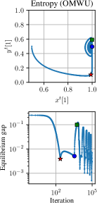
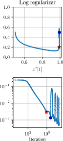
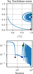
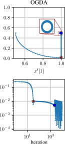
Figure 4: Comparison of the dynamics produced by three variants of OFTRL with different regularizers (negative entropy, logarithmic regularizer, and squared Euclidean norm) and OGDA in the same game $A_{\delta}$ defined in (2) for $\delta:=10^{-2}$ and adaptive step size with $\epsilon=0.1$. The bottom row shows the duality gap achieved by the iterates.

References

• Anagnostides etΒ al. [2022] Ioannis Anagnostides, Ioannis Panageas, Gabriele Farina, and Tuomas Sandholm. On last-iterate convergence beyond zero-sum games. In International Conference on Machine Learning, pages 536–581. PMLR, 2022.
• Bailey and Piliouras [2018] JamesΒ P Bailey and Georgios Piliouras. Multiplicative weights update in zero-sum games. In Proceedings of the 2018 ACM Conference on Economics and Computation, pages 321–338, 2018.
• Braverman etΒ al. [2018] Mark Braverman, Jieming Mao, Jon Schneider, and Matt Weinberg. Selling to a no-regret buyer. In Proceedings of the 2018 ACM Conference on Economics and Computation, pages 523–538, 2018.
• Brown and Sandholm [2018] Noam Brown and Tuomas Sandholm. Superhuman AI for heads-up no-limit poker: Libratus beats top professionals. Science, 359(6374):418–424, 2018.
• Cai etΒ al. [2022] Yang Cai, Argyris Oikonomou, and Weiqiang Zheng. Finite-time last-iterate convergence for learning in multi-player games. In Advances in Neural Information Processing Systems (NeurIPS), 2022.
• Cheung and Piliouras [2019] YunΒ Kuen Cheung and Georgios Piliouras. Vortices instead of equilibria in minmax optimization: Chaos and butterfly effects of online learning in zero-sum games. In Conference on Learning Theory, pages 807–834. PMLR, 2019.
• Daskalakis and Panageas [2018] Constantinos Daskalakis and Ioannis Panageas. The limit points of (optimistic) gradient descent in min-max optimization. Advances in neural information processing systems (NeurIPS), 2018.
• Daskalakis and Panageas [2019] Constantinos Daskalakis and Ioannis Panageas. Last-iterate convergence: Zero-sum games and constrained min-max optimization. In 10th Innovations in Theoretical Computer Science Conference (ITCS), 2019.
• Daskalakis etΒ al. [2018] Constantinos Daskalakis, Andrew Ilyas, Vasilis Syrgkanis, and Haoyang Zeng. Training gans with optimism. In International Conference on Learning Representations (ICLR), 2018.
• Daskalakis etΒ al. [2021] Constantinos Daskalakis, Maxwell Fishelson, and Noah Golowich. Near-optimal no-regret learning in general games. Advances in Neural Information Processing Systems (NeurIPS), 2021.
• Duchi etΒ al. [2011] John Duchi, Elad Hazan, and Yoram Singer. Adaptive subgradient methods for online learning and stochastic optimization. Journal of machine learning research, 12(7), 2011.
• Farina etΒ al. [2021] Gabriele Farina, Christian Kroer, and Tuomas Sandholm. Faster game solving via predictive blackwell approachability: Connecting regret matching and mirror descent. In Proceedings of the AAAI Conference on Artificial Intelligence, 2021.
• Farina etΒ al. [2022] Gabriele Farina, Chung-Wei Lee, Haipeng Luo, and Christian Kroer. Kernelized multiplicative weights for 0/1-polyhedral games: Bridging the gap between learning in extensive-form and normal-form games. In International Conference on Machine Learning (ICML), pages 6337–6357, 2022.
• Flaspohler etΒ al. [2021] GenevieveΒ E Flaspohler, Francesco Orabona, Judah Cohen, Soukayna Mouatadid, Miruna Oprescu, Paulo Orenstein, and Lester Mackey. Online learning with optimism and delay. In International Conference on Machine Learning, pages 3363–3373. PMLR, 2021.
• Golowich etΒ al. [2020a] Noah Golowich, Sarath Pattathil, and Constantinos Daskalakis. Tight last-iterate convergence rates for no-regret learning in multi-player games. Advances in neural information processing systems (NeurIPS), 2020a.
• Golowich etΒ al. [2020b] Noah Golowich, Sarath Pattathil, Constantinos Daskalakis, and Asuman Ozdaglar. Last iterate is slower than averaged iterate in smooth convex-concave saddle point problems. In Conference on Learning Theory (COLT), 2020b.
• Gorbunov etΒ al. [2022] Eduard Gorbunov, Adrien Taylor, and Gauthier Gidel. Last-iterate convergence of optimistic gradient method for monotone variational inequalities. In Advances in Neural Information Processing Systems, 2022.
• Hart and Mas-Colell [2000] Sergiu Hart and Andreu Mas-Colell. A simple adaptive procedure leading to correlated equilibrium. Econometrica, 68(5):1127–1150, 2000.
• Hsieh etΒ al. [2019] Yu-Guan Hsieh, Franck Iutzeler, JΓ©rΓ΄me Malick, and Panayotis Mertikopoulos. On the convergence of single-call stochastic extra-gradient methods. Advances in Neural Information Processing Systems, 32, 2019.
• Hsieh etΒ al. [2021] Yu-Guan Hsieh, Kimon Antonakopoulos, and Panayotis Mertikopoulos. Adaptive learning in continuous games: Optimal regret bounds and convergence to nash equilibrium. In Conference on Learning Theory, pages 2388–2422. PMLR, 2021.
• Koolen etΒ al. [2010] WouterΒ M Koolen, ManfredΒ K Warmuth, Jyrki Kivinen, etΒ al. Hedging structured concepts. In COLT, pages 93–105. Citeseer, 2010.
• Kumar etΒ al. [2024] Rachitesh Kumar, Jon Schneider, and Balasubramanian Sivan. Strategically-robust learning algorithms for bidding in first-price auctions. In Proceedings of the 2024 ACM Conference on Economics and Computation, 2024.
• Lee etΒ al. [2021] Chung-Wei Lee, Christian Kroer, and Haipeng Luo. Last-iterate convergence in extensive-form games. Advances in Neural Information Processing Systems, 34:14293–14305, 2021.
• Luo [2022] Haipeng Luo. Lecture note 2, Introduction to Online Learning. 2022. URL https://haipeng-luo.net/courses/CSCI659/2022_fall/lectures/lecture2.pdf.
• Mertikopoulos etΒ al. [2018] Panayotis Mertikopoulos, Christos Papadimitriou, and Georgios Piliouras. Cycles in adversarial regularized learning. In Proceedings of the twenty-ninth annual ACM-SIAM symposium on discrete algorithms, pages 2703–2717. SIAM, 2018.
• Mertikopoulos etΒ al. [2019] Panayotis Mertikopoulos, Bruno Lecouat, Houssam Zenati, Chuan-Sheng Foo, Vijay Chandrasekhar, and Georgios Piliouras. Optimistic mirror descent in saddle-point problems: Going the extra (gradient) mile. In International Conference on Learning Representations (ICLR), 2019.
• Mokhtari etΒ al. [2020] Aryan Mokhtari, AsumanΒ E Ozdaglar, and Sarath Pattathil. Convergence rate of $\mathcal{O}(1/k)$ for optimistic gradient and extragradient methods in smooth convex-concave saddle point problems. SIAM Journal on Optimization, 30(4):3230–3251, 2020.
• Munos etΒ al. [2023] RΓ©mi Munos, Michal Valko, Daniele Calandriello, MohammadΒ Gheshlaghi Azar, Mark Rowland, ZhaohanΒ Daniel Guo, Yunhao Tang, Matthieu Geist, Thomas Mesnard, Andrea Michi, etΒ al. Nash learning from human feedback. arXiv preprint arXiv:2312.00886, 2023.
• Perolat etΒ al. [2022] Julien Perolat, Bart DeΒ Vylder, Daniel Hennes, Eugene Tarassov, Florian Strub, Vincent deΒ Boer, Paul Muller, JeromeΒ T Connor, Neil Burch, Thomas Anthony, etΒ al. Mastering the game of stratego with model-free multiagent reinforcement learning. Science, 378(6623):990–996, 2022.
• Rakhlin and Sridharan [2013] Sasha Rakhlin and Karthik Sridharan. Optimization, learning, and games with predictable sequences. Advances in Neural Information Processing Systems, 2013.
• Syrgkanis etΒ al. [2015] Vasilis Syrgkanis, Alekh Agarwal, Haipeng Luo, and RobertΒ E Schapire. Fast convergence of regularized learning in games. Advances in Neural Information Processing Systems (NeurIPS), 2015.
• Takimoto and Warmuth [2003] Eiji Takimoto and ManfredΒ K Warmuth. Path kernels and multiplicative updates. The Journal of Machine Learning Research, 4:773–818, 2003.
• Tammelin etΒ al. [2015] Oskari Tammelin, Neil Burch, Michael Johanson, and Michael Bowling. Solving heads-up limit texas hold’em. In Twenty-fourth international joint conference on artificial intelligence, 2015.
• van Erven [2021] Tim van Erven. Why FTRL is better than online mirror descent. https://www.timvanerven.nl/blog/ftrl-vs-omd/, 2021. Accessed: 2024-05-22.
• Vlatakis-Gkaragkounis etΒ al. [2020] Emmanouil-Vasileios Vlatakis-Gkaragkounis, Lampros Flokas, Thanasis Lianeas, Panayotis Mertikopoulos, and Georgios Piliouras. No-regret learning and mixed nash equilibria: They do not mix. Advances in Neural Information Processing Systems, 33:1380–1391, 2020.
• Wei etΒ al. [2021] Chen-Yu Wei, Chung-Wei Lee, Mengxiao Zhang, and Haipeng Luo. Linear last-iterate convergence in constrained saddle-point optimization. In International Conference on Learning Representations (ICLR), 2021.
• Zinkevich etΒ al. [2007] Martin Zinkevich, Michael Johanson, Michael Bowling, and Carmelo Piccione. Regret minimization in games with incomplete information. Advances in neural information processing systems, 20, 2007.