String Partition for Building Big BWTs

Abstract

The Burrows-Wheeler transform (BWT) is a reversible text transformation used extensively in text compression, indexing, and bioinformatics, particularly in the alignment of short reads. However, constructing the BWT for long strings poses significant challenges. We introduce a novel approach to partition a long string into shorter substrings, enabling the use of multi-string BWT construction algorithms to process these inputs. The approach partitions based on a prefix of the suffix array and we provide an implementation for DNA sequences. Through comparison with state-of-the-art BWT construction algorithms, we demonstrate a speed improvement of approximately $12\%$ on a real genome dataset consisting of $3.2$ billion characters. The proposed partitioning strategy is applicable to strings of any alphabet.

1 Introduction

The Burrows-Wheeler transform (BWT) [3] is a widely used reversible string transformation with applications in text compression [7], indexing [7], and short read alignment [11]. The BWT reduces the number of equal-symbol runs for data compressed with run-length encoding and allows pattern searching in time proportional to the pattern length [7]. Because of these advantages, and the property that the BWT of a string $S$ can be constructed and reverted in $\mathcal{O}(S)$ time and space, the BWT is important in computational biology.

In computational biology, there are at least two major BWT construction cases: The BWT can be generated either for a single long genome, for example, the reference genome [11], or for a set of comparatively short reads [1]. The standard way to define and compute a text index for a set $W$ of strings $W_{i}$ is to concatenate the $W_{i}$ with different end-marker symbols $\#_{i}$ between the $W_{i}$ [4]: $W_{0}\#_{0}W_{1}\#_{1}\dots W_{k}\#_{k}$. We use the $\#_{i}$ or $\#$ symbols to separate the short strings from each other in the multi-string BWT construction and use the $\$$ symbol only at the end of a single word. BWT construction algorithms like BCR [1] and ropebwt2 [12] use this concatenation. If only one string $S$ or a small collection of long strings is given, the BWT of the set $\{S\}$ cannot be computed efficiently by an approach like BCR [1]. Concretely, BCR inserts each symbol of $S$ separately and does not improve by inserting multiple positions at once.

In this paper, we show how to partition a string $S$ into a set $W$ of short strings $W_{0},\dots,W_{k}$ such that the BWT of $W$ is similar to the BWT of $S$. We say ‘similar’ here because the BWT of $W_{0},\dots,W_{k}$ contains $k+1$ $\#$ symbols that we need to remove from the BWT after construction. For example, compare the BWT of

$$S=CAAAACAAACCGTAAAACAAACCGGAACAA\$$$

to the BWT of the set $W=\{W_{0},\dots,W_{8}\}$ of words

$$W_{0}=A,W_{1}=A,W_{2}=AAACCGGAAC,W_{3}=AAACCGT,$$

$$W_{4}=\$C,W_{5}=A,W_{6}=A,W_{7}=AAAC,W_{8}=AAAC.$$

Because $W_{4}W_{6}W_{8}W_{3}W_{5}W_{7}W_{2}W_{1}W_{0}\$=\$S$, $W$ is a partition of the first right rotation of $S$. The BWT of $W$ is constructed using $W_{0},\dots,W_{k}$ in the order of their indices:

$$BWT(S)=$$

$$AACTCAACC\phantom{\#\#\#\#\#\#\#\#\#{}}GAAAAAAAAAA\$AAAACCGCCG$$

$$BWT(W)=$$

$$AACTCAACC\#\#\#\#\#\#\#\#\#{}GAAAAAAAAAA\$AAAACCGCCG.$$

If we remove the consecutive sequence of $\#$ symbols, the BWTs of $S$ and $W$ are identical. In Figure 1, we show the connection between single-word and multi-string BWT construction algorithms and the contribution of our paper.

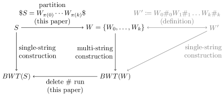
Figure 1: Summary of the relationship of single-string and multi-string BWT construction algorithms and the contribution of this paper. The multi-string construction algorithms insert new $\#$ symbols. Deleting the run of $\#$ symbols after BWT construction yields the same BWT for $S$ as shown in Theorem 4.1. The order of the words $W_{0},\dots,W_{k}$ needed to get $S$ depends on $S$, thus there exists a permutation $\pi$ of the indices.

Herein, our main contributions are:

• The proof of the correctness of partitioning an input using a prefix of the suffix array.

• An implementation partDNA to partition long DNA sequences for BWT construction.

• A comparison of state-of-the-art BWT construction algorithms with regard to the construction time advantage of using the partition.

2 Related Work

The BWT [3] is fundamental to many applications in bioinformatic such as short read alignment. Bauer et al. [1] designed BCR for a set of short DNA reads. BCR inserts all sequences at the same time starting at the end of each sequence. The position to insert the next symbol of each sequence is calculated from the current position and the constructed part of the BWT. The BWT is partitioned into buckets where one bucket contains all BWT symbols of suffixes starting with the same character. The buckets are saved on disk. ropebwt, ropebwt2, and ropebwt3 by Li [12] are similar to BCR, but use $B+$ trees instead of linear saved buckets.

The BWT can be obtained from the suffix array by taking the characters at the position before the suffix. Thereby, suffix array construction algorithms (SACA) like divsufsort, SA-IS by Nong et al. [16], gSACA-K by Louza et al. [13], or gsufsort by Louza et al. [14] can be used to obtain the BWT. Many SACAs rely on induced suffix sorting. By induced suffix sorting, we derive the order of the previous positions, if these point to equal characters, from a sorted set of suffix positions.

The grlBWT method by Díaz-Domínguez et al. [5] uses induced suffix sorting, but additionally uses run-length encoding and grammar compression to store intermediate results and to speed up computations required for BWT construction.

eGap by Egidi et al. [6] divides the input collection into small subcollections and computes with gSACA-K [13] the BWT for the subcollection. Thereafter, eGap merges the subcollection BWTs into one BWT.

In prefix-free sets, no two words from the set are prefixes of each other; thus, their order is based on a different character rather than word length. Consequently, the order of two suffixes prefixed by words from the prefix-free set is determined by these words. BigBWT by Boucher et al. [2] builds the BWT using prefix-free sets. BigBWT replaces the input by a dictionary D and a parse P using the rolling Karp-Rabin hash. P is the list of entries in D according to the input string, D forms a prefix-free set. r-pfbwt by Oliva et al. [17] recursively uses prefix free parsing on the parse P to further reduce the space needed to represent the input string.

String partitioning is common before BWT construction. SA-IS [16], gSACA-K [13], BigBWT [2] and r-pfbwt[17] all partition the input at LMS-Positions or by using a dictionary. Another use case is the bijective BWT, which uses the partition in Lyndon Words [10].

The difference of our partition to all these approaches is that we do not create a BWT as a result. Instead, we translate the problem into a multi-string BWT construction problem and compute the BWT using such a construction method.

3 Preliminaries

We define a string $S$ of length $|S|\coloneqq n$ over $\Sigma$ by $S=a_{0}a_{1}\cdots a_{n-1}a_{n}$ with $a_{i}\in\Sigma$ for $i<n$ and $a_{n}=\$$. We write $S[i]=a_{i}$, $S[i,j]=a_{i}a_{i+1}\cdots a_{j}$ for a substring of $S$, and $S[i..]=S[i,n]$ for the suffix starting at position $i$. For simplicity, we assume that $S[-1]=S[n]=\$$, and also allow $S[-1,j]=a_{n}a_{0}\cdots a_{j}$ as a valid interval.

The suffix array $SA(S)$ [15] is a permutation of $\{0,\ldots,n\}$ such that the $i$-th smallest suffix of $S$ is $S[SA(S)[i]..]$. In case we have an ordered set $W$ of strings $W_{j}$, the document array $DA(W)$ is used along with the suffix array in order to describe to which word $W_{x}$ the $i-th$ suffix array entry $SA(W)[i]$ belongs. That is, $DA(W)[i]=x$ denotes that the $i$-th suffix array entry $SA(W)[i]$ belongs to the word $W_{x}$. So, the $i$-th smallest suffix of $W$ is $W_{DA(W)[i]}[SA(W)[i]..]$.

The Burrows–Wheeler transform $BWT(S)$ [3] of a string $S$ can either be obtained by taking the last column of the sorted rotations of $S$ or by

$$BWT(S)[i]=S[SA[i]-1].$$

4 Partition Theorem

A single string $S$ has only unique suffixes, because the suffixes differ in their length. If we partition $S$ into $W=\{W_{0},\dots,W_{k}\}$, $W_{0},\dots,W_{k}$ can have several equal suffixes. For example, $W_{2}=AAACCGGAAC$ and $W_{7}=AAAC$ both have the suffix $AAC$. Given only the suffixes, we cannot decide how to order the characters $G$ and $A$ in $BWT(W)$ that occur before the suffixes $AAC$ in $W_{2}$ and $W_{7}$. We break the tie by the word order of $W_{2}$ and $W_{7}$ that we define to be the order of the suffixes occuring in $S$ after $W_{2}$ and $W_{7}$.

Instead of arguing with suffixes, we can use suffix arrays: The index $i$ of a word $W_{i}$ is the index $i$ within a suffix array that only contains the positions in $S$ after the words of $W$. Computing the full suffix array and thereafter filtering it for the positions that follows the word ends yields the correct order of the words. However, if we would construct the full suffix array to partition $S$, this were inefficient because we can obtain the BWT from the suffix array directly. But this trivial solution shows we can obtain the word indices in $\mathcal{O}(n)$.

In multi-string construction of $BWT(W)$, the last characters $c_{0},\dots,c_{k}$ of each word $W_{0},\dots,W_{k}$ are inserted at the first positions of the BWT of $W$; thus, $c_{0},\dots,c_{k}$ must be the first $k+1$ symbols of $BWT(S)$. Thereby, the positions in $S$ following the words $W_{0},\dots,W_{k}$ form a continuous block at the lowest positions of the suffix array of $S$: A prefix of the suffix array.

We define $PSA(S)=SA(S)[0\dots k]$ as a prefix of a length $k+1$ of the suffix array of $S$. In the following, we assume $k$ to be a fixed value. We write $t\in PSA(S)$, if the exact position of $t$ is unimportant and only the occurrence of $t$ in $PSA(S)$ is important.

For each suffix entry $PSA(S)[j]$, let $\Omega(j)=\max(\{-1\}\cup\{t\in PSA(S):t\leq PSA(S)[j]-1\})$ be the next smaller suffix array entry in $PSA(S)$ or $-1$, if the $PSA(S)$ value is already the smallest one. We define $W$ as the ordered set of words $W_{i}=S[\Omega(i),PSA(S)[i]-1]$ for $0\leq i\leq k$, which is a partition of the first right rotation of $S$ into substrings.

As $W$ is a partition of the first right rotation of $S$, each character of $S$ is mapped to exactly one character in $W$, so we define two functions $word$ and $position$ to map a position $q$ from $S$ to the corresponding place of that character $S[q]$ in $W$. For each $q$ with $-1\leq q<|S|$ exists exactly one $j\leq k$ such that $q\in[\Omega(j),PSA(S)[j]-1]$, because each position in the partition belongs to exactly one interval. We set $word(q)=j$ and $position(q)=q-\Omega(j)$. We also set $word(n)=word(-1)$ and $position(n)=position(-1)$.

In the initial example, the $C$ at position $0$ in $S$ corresponds to the $C$ in word $W_{4}$ at position $1$, so $word(0)=4$ and $position(0)=1$.

In the edge cases for $k$ in the $PSA(S)$ definition, we obtain for $k=0$ that the prefix of the suffix array only contains the position of the $\$$ symbol, which is at the end of the word. It follows $\Omega(n)=-1$, because $\{i\in PSA(S):i<PSA(S)[i]\}=\emptyset$. Thereby, $W$ contains only one word which is $W_{0}=S[\Omega(i),PSA(S)[i]-1]=S[-1,n-1]$, which is the first right rotation of $S$. Using the $\$$ as end marker, the BWTs of $S$ and $W$ are equal, because the suffixes have not changed.

For the edge case $k=n$, $PSA(S)=SA(S)$ and $\{i\in PSA(S):i<PSA(S)[i]-1\}=\{0,\dots,PSA(S)[i]-1\}$ because the suffix array contains all positions of $S$. Thereby, we get $\Omega(i)=PSA(S)[i]-1$ for all positions $i$, so

$$W_{i} =S[\Omega(i),PSA(S)[i]-1]$$

$$=S[PSA(S)[i]-1,PSA(S)[i]-1]$$

$$=S[PSA(S)[i]-1]$$

$$=S[SA(S)[i]-1]$$

$$=BWT(S)[i].$$

Each word is one symbol and their order is already the BWT of $S$, because the order is obtained from the suffix array of $S$. If we construct the BWT from the words in this edge case, it is easy to see that $BWT(W)=BWT(S)+\#^{n}$.

Theorem 4.1

Let $S$ be a string of length $n$ over the alphabet $\Sigma$. Let $W$ be the ordered set of partitioned words $W_{i}=S[\Omega(i),PSA(S)[i]-1]$ obtained from $S$. Let $l(=k+1)$ be the size of $W$, $m(=n+l)$ be the total length of $BWT(W)$, and let $BWT(S)$ and $BWT(W)$ be the BWTs of $S$ and $W$, respectively. Then, for all $i<m$:

$$BWT(W)[i]=\begin{cases}BWT(S)[i]&0\leq i<l\\ \#&l\leq i<2l\\ BWT(S)[i-l]&2l\leq i<m\end{cases}$$

The proof of Theorem 4.1 is in Appendix A.

5 Partition DNA Sequences: partDNA

Next, we partition DNA sequences because reference genomes are long strings over $ACGT$, for example, the human genome is about 3.2 billion characters. The suffix array construction algorithm by Rabea et al. [18] constructs the suffix array for a set of DNA reads incrementally starting at the smallest substring, so by stopping their SACA any length of a prefix of the suffix array for a given DNA sequence can be obtained. For larger alphabets, the external approach of Kärkkäinen [9] can be adjusted to get a prefix of the suffix array.

Obtaining the value $\Omega(j)$ from an already sorted prefix of the suffix array $sort(PSA(S))$ is less computational expensive than getting the $\Omega(j)$ from $PSA(S)$, because the next lower entry of $q=sort(PSA(S))[i]$ with $i>0$ is $\Omega(j)=sort(PSA(S))[i-1]$, or in case of $i=0$, $\Omega(j)=-1$. Therefore, given $sort(PSA(S))$ and the permutation from $sort(PSA(S))$ to $PSA(S)$, we get the partition of $S$ with $PSA(S)$ with less computational cost. In other words, to partition a DNA sequence $S$, we

• find the words having the smallest suffixes in $S$, and

• we order the words according to their suffixes in $S$.

To simplify the computation of $sort(PSA(S))$, we do not allow every $k$ as length of the prefix of the suffix array and $k$ is not given explicitly. Instead, the exact value of $k$ will be part of the result of the partition. We use the length $h$ for the chosen minimal length of an $A$ run as a parameter to partition $S$.

For example, we partition

$$S=CAAAACAAACCGTAAAACAAACCGGAACAA\$$$

with $h=3$. The example is visualized in Figure 2.

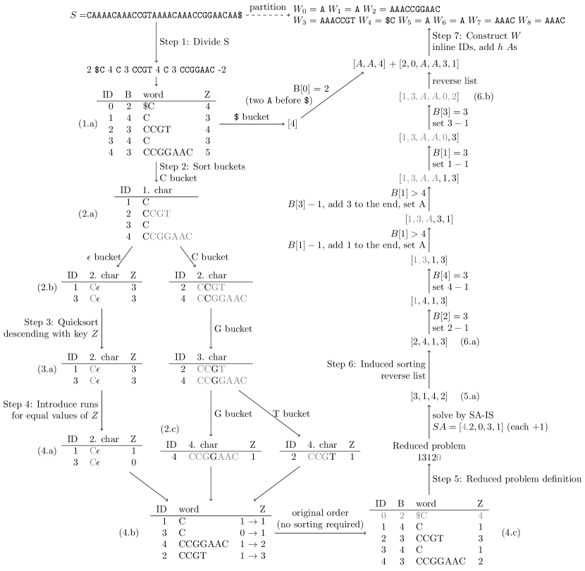
Figure 2: Example calculation of partitioning using $h=3$ on the word $S$. We only reorder the IDs, the reordering of all other elements is only shown for illustration. The sorting in Step 2 is done in place, so there is no action from (4.a) and (2.c) to (4.b) necessary.

In Step 1, we divide $S$ before each sequence of at least $h$ $A$ symbols or any sequence of $A$s followed by the $\$$ symbol. Additionally, we avoid writing the $A$s at the start or end of a word, we only save the run-length of $A$ symbols. This results in less words than the final partition has, because we obtain the other words by induced suffix sorting as shown in Figure 3. We keep the number of $A$s before each word in an array $B$ and the number of $A$s after each word in an array $Z$. When we reach the $\$$ symbol, we keep the length of the current A run in $B[0]$, so in the example of Figure 2, $B[0]=2$, and we store the maximum length of an $A$ run plus 1 in the last element of $Z$ regardless of how long the current $A$ run is, so in the example, $Z[4]=5$. We use these values of $Z$ later to sort the words accordingly. We put the $\$$ at the start of the word with ID $0$.

In Step 2, we sort the IDs of Figure 2 (1.a) with a value of $1$ and greater. The arrays $B$ and $Z$ and the words in Figure 2 (1.a) are only accessed indirectly and changed by using $B[ID[i]]$ and $Z[ID[i]]$. We sort the IDs by recursively refining buckets; therefore, the idea is similar to bucket sort. The call structure is a tree as shown in Figure 2 (2.a) to (2.c), that has a maximum number of 5 branches that continue sorting on each level, one for each character $A$, $C$, $G$, and $T$ and one branch named $\epsilon$ for the case that we have reached the end of a word.

If a word $w$ has no character at the current depth within the sort tree, we reached $\epsilon$-leaf of the search tree for $w$. Then, $w$ is lexicographic smaller than the words that have a character at that position, because in $S$, after $w$ occurs a pattern $A^{h+y}$ or the lexicographicly even smaller suffix $A^{y}\$$ with $y\geq 0$. Because we used different patterns to partition $S$, we sort with quicksort the words according to the order of these patterns as Step 3. In Figure 2 (1.a), the patterns $A^{3}$, $A^{4}$, and $A^{2}\$$ are encoded by the values $3$, $4$, and $5$ in the array $Z$. A shorter run of $A$ before a $\$$ is a smaller pattern than a longer run of $A$ before a $\$$, any $A^{w}\$$ is a smaller pattern than any $A^{v}$, and a longer run of $A$s not terminated by a $\$$ is smaller than a shorter run of $A$s not terminated by a $\$$. Therefore, the quicksort sorts the IDs in descending order by using the values in $Z$ as keys.

After the quicksort in the leaves of the sort tree, we might have identical words as in Figure 2 (3.a). In the leaf, two words are equal if they appear consecutively and their value in $Z$ is equal. In Step 4, we encode equal words as a run, so the first of the equal words gets a $1$ and each other word gets a $0$ in $Z$. This allows an easier assignment of names in the following step. All words in leaves containing only one word get a $1$ in $Z$ like in Figure 2 (2.c).

To solve the case that we found at least two equal words in Step 4, we define a reduced suffix array construction problem to sort them. In Figure 2 (4.a), the words with IDs 1 and 3 are equal. The reduced problem is defined as in SA-IS [16] and similar SACAs. In a single pass over $Z[ID[i]]$, we give integer names to the words, like in Figure 2 (4.b). We add the current value of $Z$, which is $0$ or $1$, to the last name and then assign the sum to $Z$. The smallest assigned name is $1$, because we use $0$ as a global end marker for a valid suffix array problem definition.

In Step 5, we obtain the reduced problem by reading the names from $Z[i]$. Again, we omit the first word with ID $0$.

In Figure 2, the reduced problem is $R=13120$, with the global end marker $0$. We compute $SA(R)$ with SA-IS [16]. In Appendix B, we show that $R$ is smaller than the recursive problem in SA-IS for the same input. $SA(R)=[4,2,0,3,1]$. We omit the first value $4$, because the $4$ points towards the end marker $0$. We need to add $1$ to the $SA(R)$ values, because we skipped the word with ID $0$ in the recursive problem. We obtain $[3,1,4,2]$ (Figure 2 (6.a)).

In Step 6, we obtain all words from the sorted IDs by induced suffix sorting. Figure 3 shows the possible induced suffix sorting steps. Let $L$ be the list of IDs in inverted order, so $L=[2,4,1,3]$. We iterate from the start until we reach the end of $L$. For the ID $j$, if $B[j]$ is greater than $h$: We reduce $B[j]$ by 1, write an $A$ to the current position of the list and append the current ID $j$ to the end of the list again. If $B[j]$ is $h$: We reduce $j$ by $1$ at the current position because we sorted suffixes. We get $L=[1,3,A,A,0,2]$ (Figure 2 (5.b)) and invert the list again, so $L=[2,0,A,A,3,1]$. This step is the induced suffix sorting step from SA-IS [16].

Figure 3: The buckets and the steps of induced suffix sorting that start and end inside the displayed interval. The name of a bucket is a shared prefix of the suffixes. For the $A^{v}$ buckets it is required that the next symbol is not an $A$, otherwise the $AAA$ and $AAAA$ bucket would also belong to the $AA$ bucket. We induce the positions from the $\$$ bucket to the next bucket on the right and reduce the suffix array entry by 1 if and only if the symbol at the position before the entry is an $A$, which is the symbol in the BWT row. In the same way, we can fill the $A^{v}$ buckets right to left.

For the $\$$-bucket, we also use induced sorting: The starting list is $Q=[4]$ because the word with ID $4$ in Figure 2 (1.a) of the partitioned words has $A^{B[0]}\$$ as a suffix and we do $B[0]$ steps each inserting one $A$. The result is $Q=[A,A,4]$ and the combined result is $Q+L$.

In Step 7, each $A$ in $Q+L$ yields an own word $W_{i}=A$. Each ID in $Q+L$ yields the corresponding word in Figure 2 (1.a). Additionally, in front of each word with an ID that is $1$ or greater in Figure 2 (1.a), we prepend $h$ $A$s. After Step 7, we get the partition:

$$W_{0}=A,W_{1}=A,W_{2}=AAACCGGAAC,W_{3}=AAACCGT,$$

$$W_{4}=\$C,W_{5}=A,W_{6}=A,W_{7}=AAAC,W_{8}=AAAC.$$

To summarize: By partitioning $S$ into the set $W=\{W_{0},\dots,W_{8}\}$, we have transformed the task of constructing the BWT of a long string $S$ into the task of constructing the BWT of a set $W$ of smaller words which can be solved faster for very long strings $S$.

6 Experimental Results

We compare the BWT construction algorithms listed in Table 2 on the original and partitioned datasets, which are listed in Table 1. We performed all tests on a Debian 5.10.209-2 machine with 128GB RAM and 32 Cores Intel(R) Xeon(R) Platinum 8462Y+ @ 2.80GHz.

dataset	$h$	max length	average length	set size $l$
Chromosome 1 of GRCh38	$-$	230481012	230481012.00	1
Chromosome 1 of GRCh38	1	668	4.44	67070278
Chromosome 1 of GRCh38	2	4814	11.52	21901549
Chromosome 1 of GRCh38	3	5994	28.06	8516549
Chromosome 1 of GRCh38	4	18514	68.30	3424459
Chromosome 1 of GRCh38	5	32963	153.26	1513744
Chromosome 1 of GRCh38	6	177049	294.24	785969
Chromosome 1 of GRCh38	7	597800	450.79	512423
Chromosome 1 of GRCh38	8	1690534	609.89	378528
Chromosome 1 of GRCh38	9	2782481	761.50	303067
Chromosome 1 of GRCh38	uh10	2782482	926.28	249094
GRCh38	$-$	uhh3136819154	uhh3136819154.00	1
GRCh38	3	25230	26.29	uhh119294890

Table 1: GRCh38 can be obtained from NCBI (https://www.ncbi.nlm.nih.gov/). Ambiguous bases are filtered out before. The GRCh38 is a concatenation of all bases of the reference genome file. If a partition length $h$ is provided, the dataset was partitioned using $h$ from the dataset without a partition length $h$.

The partition of the datasets allows different formulations of the same BWT construction problem. In Table 1, all entries of chromosome 1 have the same BWT except for the $\#$ run, but have different characteristics regarding the length of the longest input string of the collection, the average length of strings in the collection, and the collection size, which is $l$ in Theorem 4.1. Also, all sets for the concatenated GRCh38 file have the same BWT except for the $\#$ run. The size of the prefix of the suffix array that was used to partition a set is equal to the set size value.

approach	paper	implementation
BCR	[1]	https://github.com/giovannarosone/BCR_LCP_GSA
ropebwt	$-$	https://github.com/lh3/ropebwt
ropebwt2	[12]	https://github.com/lh3/ropebwt2
ropebwt3	$-$	https://github.com/lh3/ropebwt3
BigBWT	[2]	https://github.com/alshai/Big-BWT
r-pfbwt	[17]	https://github.com/marco-oliva/r-pfbwt
divsufsort	([8])	https://github.com/y-256/libdivsufsort
grlBWT	[5]	https://github.com/ddiazdom/grlBWT
eGap	[6]	https://github.com/felipelouza/egap
gsufsort	[14]	https://github.com/felipelouza/gsufsort

Table 2: BWT construction algorithms compared.

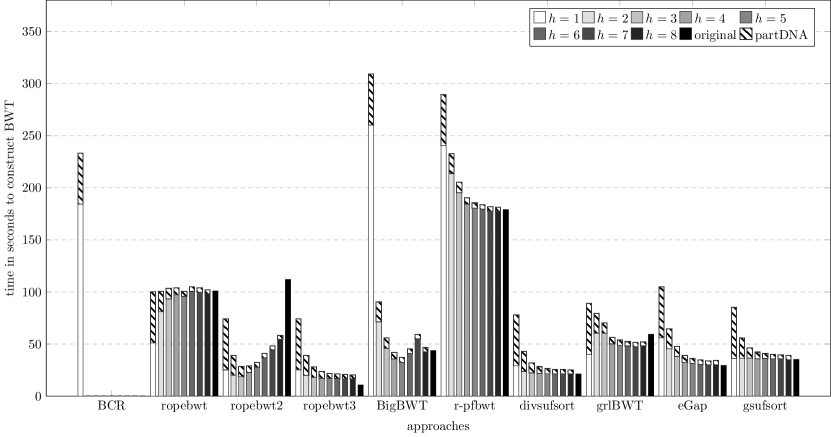
Figure 4: BWT construction time for GRCh38 chromosome 1. Each approach is tested on the partitioned datasets. BCR failed to process any other than $h=1$ file failing the assertion $num\_write==charsBuffered-1$. BCR occupies more than 200GB of hard disc space for its cyc files, which may cause the exception.

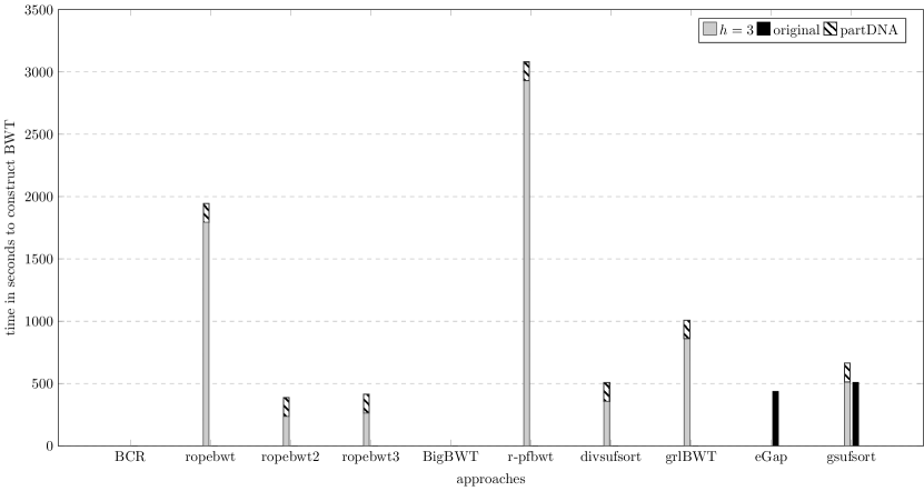
Figure 5: BWT construction time for the full concatenated GRCh38. A missing bar means that the approach was not able to construct the BWT, for example the assertion $tot\_char==size$ lets BigBWT fail. eGap uses for the original dataset only a chunk count of $1$, so the BWT is completely constructed by gSACA-K [13].

Partitioning only improves approaches that gain advantage of an input with multiple strings. Approaches that define the multi-string BWT construction by concatenating the strings into one string to process them, now need to process a bigger input due to the additionally added $\#$ symbols. Hence, we expect for example BigBWT and r-pfbwt to slow down.

In Figure 4, ropebwt3 is the fastest approach on the original one-genome dataset, taking about 10.6 seconds. ropebwt3 outperforms ropebwt2, which constructs the BWT in about 18.6 seconds plus 10.0 seconds to partition the input using $h=3$, so 28.5 seconds total.

The runtime improvement for the concatenated GRCh38 file with about 3.2 billion symbols is shown in Figure 5. ropebwt2 with 387.9 seconds is about 50 seconds faster than eGap on the original file with 437.5 seconds, which is about $12\%$ faster. Of the 387.9 seconds of ropebwt2, the partition took 151.0 seconds, which are $38.9\%$ of the total construction time using ropebwt2. Additionally, we highlight that many approaches are not able to process the original file but are able to handle the partitioned file.

7 Conclusion

We have presented an approach to partition long strings in order to transform a long string BWT construction problem into a multi-string BWT construction problem. This enables multi-string BWT construction algorithms to construct BWTs which they were not capable to construct before. We have shown that our implementation partDNA provides a speed improvement of about $12\%$ on a real genome dataset of $3.2$ billion characters. In addition, the partition works on strings of any alphabet; thus, our future research includes computing the prefix of a suffix array for other alphabets than genomes.

Appendix A: Proof of the Partition Theorem

Proposition 1

For any $q$ with $-1\leq q<n$: if $q\in PSA(S)$ or $q=-1$, then

$$position(q)=0.$$

Proof

$SA[0]=n$, because $S[n]=\$$ is by definition the smallest symbol and unique, thereby, $n$ is the index of the smallest suffix. Let $p$ be the $\min(\{t\in PSA(S):t>q\})$ which is well defined, because $q<n$ and $n\in PSA(S)$ for any $k\geq 0$. Then $q=\Omega(p)$ and $q\in[\Omega(p),PSA(S)[p]-1]$, so $position(q)=q-\Omega(p)=q-q=0$.

Proposition 2

For any $q$ with $0\leq q<n$: if $q\not\in PSA(S)$, then

$$word(q)=word(q-1)\text{ and }position(i-1)=position(i)-1.$$

Proof

If $position(q)=0=q-\Omega(j)$ for a $j$, it follows $\Omega(j)=q$, so $q\in\{-1\}\cup PSA(A)$, which contradicts the assumptions. Thereby, $\Omega(j)<q<PSA(j)-1$, from this we get $\Omega(j)\leq q-1<PSA(j)-1$, so $word(q-1)=word(q)$. $position(q-1)=q-1-\Omega(j)=q-\Omega(j)-1=position(q)-1$.

We define $W^{\prime}_{i}=W_{i}+\#_{i}$ and use the $W^{\prime}_{i}$ in the proofs, because $BWT(W)$ contains $k$ $\#$ symbols that the $W_{i}$ do not contain. The lexicographical order is $\#_{0}<\#_{1}<\cdots<\#_{k}<\$<a$ for all $a\in\Sigma$. The advantage of using the $W^{\prime}_{i}$ is, that their total length is equal to the length of $BWT(W)$. Thus, we can write down the suffix array for the $W^{\prime}_{i}$ that fits to $BWT(W)$, which is not possible for the $W_{i}$. The advantages of using the $W_{i}$ in the previous part of the paper are the easier presentation of the partition of $S$ and the definition of a multi-string problem as in Figure 1. We add the index $i$ to the $\#$ symbols in order to break the tie of equal suffixes at the $\#$ symbols.

Proposition 3

If $S[i..]<S[j..]$, then

$$W^{\prime}_{word(i)}[position(i)..]<W^{\prime}_{word(j)}[position(j)..].$$

Proof

Let $c\geq 0$ be the smallest value for which either $S[i+c]\neq S[j+c]$, or $i+c\in PSA(S)$, so $S[i,i+c-1]=S[j,j+c-1]$. The idea here is, that $c$ is the distance to the positions where the tie between the suffixes starting at $i$ and $j$ breaks. First, from $S[i,i+c-1]=S[j,j+c-1]$ and $S[i..]<S[j..]$, we conclude that $S[i+b..]<S[j+b..]$ for all $b$ with $0\leq b<c$. As $PSA(S)$ contains the positions of the smallest suffixes of $S$, we conclude from $i,i+1,\dots,i+c-1\not\in PSA(S)$ and $S[i+b..]<S[j+b..]$ for all $b$ with $0\leq b<c$ that $j,j+1,\dots,j+c-1\not\in PSA(S)$.

Second, by 2, we now get

$$word(i)=word(i+1)=\cdots=word(i+c-1),$$

$$word(j)=word(j+1)=\cdots=word(j+c-1),$$

$$position(i+c-1)=position(i+c-2)+1=\cdots=position(i)+c-1,$$

$$position(j+c-1)=position(j+c-2)+1=\cdots=position(j)+c-1.$$

This shows, that the tie of $position(i)$ in $W^{\prime}_{word(i)}$ in comparison to $position(j)$ in word $W^{\prime}_{word(j)}$ is not decided before the distance $c$. In other words, if we can prove $W^{\prime}_{word(i+c-1)+1}[position(i+c-1)+1..]<W^{\prime}_{word(j+c-1)+1}[position(j+c-1)+1..]$, we get $W^{\prime}_{word(i)}[position(i)..]<W^{\prime}_{word(j)}[position(j)..]$, which is what we wanted to prove.

Now, we distinguish three cases.

First case, if $S[i+c]\neq S[j+c]$ and $i+c\not\in PSA(S)$: Like above, $j+c\not\in PSA(S)$, so we get

$$W^{\prime}_{word(i+c)}[position(i+c)]=S[i+c]<S[j+c]=W^{\prime}_{word(j+c)}[position(j+c)].$$

This is the case, when the comparison of two suffixes in $W$ can be decided without getting to the end of a word in $W$.

Second case, if $i+c=PSA(S)[v]$ and $j+c\not\in PSA(S)$: Then

$$W^{\prime}_{word(i+c-1)}[position(i+c-1)+1]=\#_{v}<S[j+c]=W^{\prime}_{word(j+c)}[position(j+c)].$$

Note that $position(i+c-1)+1\geq 1$ and $position(i+c)=0$ by 1 because $word(i+c-1)\neq word(i+c)$.

Third case, if $i+c=PSA(S)[v]$ and $j+c=PSA(S)[w]$: From $S[i..]<S[j..]$, we get $v<w$ by the definition of the suffix array. Then

$$W^{\prime}_{word(i+c-1)}[position(i+c-1)+1] =\#_{v}$$

$$<\#_{w}$$

$$=W^{\prime}_{word(j+c-1)}[position(j+c-1)+1]$$

Theorem 0..1

Let $S$ be a string of length $n$ over the alphabet $\Sigma$. Let $W$ be the ordered set of partitioned words $W_{i}^{\prime}=S[\Omega(i),PSA(S)[i]-1]+\#_{i}$ obtained from $S$. Let $l(=k+1)$ be the size of $W$, $m(=n+l)$ be the total length of $W$, and let $SA(S)$ and $SA(W)$ be the suffix arrays of $S$ and $W$, respectively. Then, the suffix array and document array are (for all $i<m$):

$$SA(W)[i]=\begin{cases}|W_{i}|&0\leq i<l\\ position(SA(S)[i-l])&l\leq i<m\end{cases}$$

$$DA(W)[i]=\begin{cases}i&0\leq i<l\\ word(SA(S)[i-l])&l\leq i<m\end{cases}$$

Proof

By construction of the words $W^{\prime}_{i}$, the smallest $k+1=l$ characters in $W$ are $\#_{i}$ and each $\#_{I}$ occurs only once. Thereby, we get $SA(W)[i]=|W^{\prime}_{i}|-1=|W_{i}|$, which is the position of the $\#_{i}$ in $W^{\prime}_{i}$, together with $DA(W)[i]=i$ for $0\leq i<m$ by the order of the $\#_{i}$ symbols.

Next, there is a continuous block of length $n$ left in the $SA(W)$ and $DA(W)$ arrays to prove. By definition of the suffix array, we get for the string $S$

$$S[SA(S)[0]..]<\cdots<S[SA(S)[n-1]..].$$

By 3, we get the following order of the remaining $n$ suffixes of $W$:

$$W^{\prime}_{word(SA(S)[0])}[position(SA(S)[0])..]$$

$$< W^{\prime}_{word(SA(S)[1])}[position(SA(S)[1])..]$$

$$< \cdots$$

$$< W^{\prime}_{word(SA(S)[n-1])}[position(SA(S)[n-1])..].$$

The inequations show the order of the remaining $n$ suffixes. For example, we get that $W^{\prime}_{word(SA(S)[0])}[position(SA(S)[0])..]$ is the $l$-th lowest suffix of $W$, so $SA(W)[l]=position(SA(S)[l-l])$ and $DA(W)[l]=word(SA(S)[l-l])$. The additional $-l$ within the terms $SA(S)[i-l]$ come from the fact that this order starts at position $l$ in $SA(W)$ instead of at position $0$.

Theorem 0..1

Let $S$ be a string of length $n$ over the alphabet $\Sigma$. Let $W$ be the ordered set of partitioned words $W_{i}^{\prime}=S[\Omega(i),PSA(S)[i]-1]+\#_{i}$ obtained from $S$. Let $l(=k+1)$ be the size of $W$, $m(=n+l)$ be the total length of $BWT(W)$, and let $BWT(S)$ and $BWT(W)$ be the BWTs of $S$ and $W$, respectively. Then, for all $i<m$:

$$BWT(W)[i]=\begin{cases}BWT(S)[i]&0\leq i<l\\ \#&l\leq i<2l\\ BWT(S)[i-l]&2l\leq i<m\end{cases}$$

Proof

We calculate $BWT(W)$ from $SA(W)$. For any $i<m$:

$$BWT(W)[i]=W^{\prime}_{DA(W)[i]}[SA(W)[i]-1].$$

In the case that $i<l$, we get

$$W^{\prime}_{DA(W)[i]}[SA(W)[i]-1]=W^{\prime}_{i}[|W_{i}|-1]$$

and with the definition of $W^{\prime}_{i}$, we get

$$W^{\prime}_{i}[|W_{i}|-1]=S[PSA(i)-1]=S[SA(S)[i]-1]=BWT(S)[i].$$

In the case $i\geq l$, we get

$$W^{\prime}_{DA(W)[i]}[SA(W)[i]-1]=W^{\prime}_{word(SA(S)[i-l])}[position(SA(S)[i-l])-1].$$

Next, if $i<2l$, we have $i-l<l$, so $SA(S)[i-l]\in PSA(S)$. We can use 1 now: $position(SA(S)[i-l])=0$, hence

$$W^{\prime}_{DA(W)[i]}[SA(W)[i]-1]=W^{\prime}_{word(SA(S)[i-l])}[0-1]=\#_{word(SA(S)[i-l])}$$

Last, if $i\geq 2l$, so $SA(S)[i-l]\not\in PSA(S)$. There is exactly one $j<l$, such that $SA(S)[i-l]\in[\Omega(j),PSA(j)-1]$. Then, $position(SA(S)[i-l])=\Omega(j)-SA(S)[i-l]$ and $position(SA(S)[i-l]-1)=\Omega(j)-SA(S)[i-l]-1$ due to 2.

$$BWT(W)[i] =W^{\prime}_{word(SA(S)[i-l])}[position(SA(S)[i-l])-1]$$

$$=S[\Omega(j),PSA(j)-1][SA(S)[i-l]-1-\Omega(j)]$$

$$=S[\Omega(j)+SA(S)[i-l]-1-\Omega(j)]$$

$$=S[SA(S)[i-l]-1]$$

$$=BWT(S)[i-l].$$

In the proofs of Theorem 1 and 2, we only shown the correctness of the partition using a single word $S$, but the proofs did not use the limitation that only one string $S$ was given. The presented partitioning can also transform a set of strings $S=\{S_{0},\dots,S_{n}\}$ into a larger set of shorter words. The necessary changes for partitioning a set of strings use a suffix array and a document array of $S$ instead of using only the suffix array of $S$ and they include a set of $\$$ symbols to terminate the strings and a set of $\#$ symbols for partitioning the strings into words. Hereby, each $\$$ symbol is lexicographically larger than each $\#$ symbol. There is no change necessary in the proof steps.

If data is highly repetitive, similar words are next to each other in the ordered set $W$ after partitioning $S$. The argument is the same as for the BWT grouping similar characters together: If partitioning splits a pattern occurring frequently in $S$, each word before such a split position has a common prefix of its suffix because the split position occurs often as well. In the example of $S$, we have twice $AAAACAAACCG$. The words $AAAAC$ are grouped together by their suffixes starting with $AAACCG$.

Appendix B: On the Size of the Reduced Problem

Theorem 0..2

Each position $p>0$ with either $S[p]=A=S[p+1]=\cdots=S[p+d-1]$ and $S[p+d]\not\in\{\$,A\}$ and $S[p-1]\neq A$ or $S[p]=\$$ is a left-most S-type (LMS) position (according to the definition in SA-IS [16]).

Proof

If $S[p]=\$$: $S[p-1]\neq\$$ and thereby, $S[p-1]>S[p]$. Then $p-1$ is L-Type and $p$ is S-Type by definition, which mean that $p$ is a LMS position.

Next, $S[p]=A$. $\$\neq S[p-1]\neq A$, so $S[p-1]\in\{C,G,T\}$. We get $S[p-1]>S[p]$, so $p-1$ is L-Type. Because $S[p+d]\not\in\{\$,A\}$, $p+d-1$ is S-Type. Finally, $S[p]=A=S[p+1]=\cdots=S[p+d-1]$ implies that the type of $p$ is equal to $p+1$ is equal to $\dots$ is equal to $p+d-1$, so $p$ is S-Type and LMS-position.

We conclude that our reduced problem is smaller or equal to the recursive problem of SA-IS, because our reduced problem contains only one character for each position $p$ with $d>h$.

References

- [1] Bauer, M.J., Cox, A.J., Rosone, G.: Lightweight algorithms for constructing and inverting the BWT of string collections. Theor. Comput. Sci. 483, 134–148 (2013). https://doi.org/10.1016/J.TCS.2012.02.002
- [2] Boucher, C., Gagie, T., Kuhnle, A., Langmead, B., Manzini, G., Mun, T.: Prefix-free parsing for building big BWTs. Algorithms Mol. Biol. 14(1), 13:1–13:15 (2019). https://doi.org/10.1186/S13015-019-0148-5
- [3] Burrows, M., Wheeler, D.: A block-sorting lossless data compression algorithm. In: Digital SRC Research Report. Citeseer (1994)
- [4] Cenzato, D., Lipták, Z.: A Theoretical and Experimental Analysis of BWT Variants for String Collections. In: 33rd Annual Symposium on Combinatorial Pattern Matching, CPM 2022, June 27-29, 2022, Prague, Czech Republic. pp. 25:1–25:18 (2022). https://doi.org/10.4230/LIPICS.CPM.2022.25
- [5] Díaz-Domínguez, D., Navarro, G.: Efficient construction of the BWT for repetitive text using string compression. Inf. Comput. 294, 105088 (2023). https://doi.org/10.1016/J.IC.2023.105088
- [6] Egidi, L., Louza, F.A., Manzini, G., Telles, G.P.: External memory BWT and LCP computation for sequence collections with applications. Algorithms Mol. Biol. 14(1), 6:1–6:15 (2019). https://doi.org/10.1186/S13015-019-0140-0
- [7] Ferragina, P., Manzini, G.: Indexing compressed text. J. ACM 52(4), 552–581 (2005). https://doi.org/10.1145/1082036.1082039
- [8] Fischer, J., Kurpicz, F.: Dismantling DivSufSort. In: Proceedings of the Prague Stringology Conference 2017, Prague, Czech Republic, August 28-30, 2017. pp. 62–76 (2017), http://www.stringology.org/event/2017/p07.html
- [9] Kärkkäinen, J.: Fast BWT in small space by blockwise suffix sorting. Theor. Comput. Sci. 387(3), 249–257 (2007). https://doi.org/10.1016/J.TCS.2007.07.018
- [10] Kufleitner, M.: On Bijective Variants of the Burrows-Wheeler Transform. In: Proceedings of the Prague Stringology Conference 2009, Prague, Czech Republic, August 31 - September 2, 2009. pp. 65–79 (2009), http://www.stringology.org/event/2009/p07.html
- [11] Langmead, B., Salzberg, S.L.: Fast gapped-read alignment with Bowtie 2. Nature methods 9(4), 357–359 (2012)
- [12] Li, H.: Fast construction of FM-index for long sequence reads. Bioinform. 30(22), 3274–3275 (2014). https://doi.org/10.1093/BIOINFORMATICS/BTU541
- [13] Louza, F.A., Gog, S., Telles, G.P.: Induced Suffix Sorting for String Collections. In: 2016 Data Compression Conference, DCC 2016, Snowbird, UT, USA, March 30 - April 1, 2016. pp. 43–52 (2016). https://doi.org/10.1109/DCC.2016.27
- [14] Louza, F.A., Telles, G.P., Gog, S., Prezza, N., Rosone, G.: gsufsort: constructing suffix arrays, LCP arrays and BWTs for string collections. Algorithms Mol. Biol. 15(1), 18 (2020). https://doi.org/10.1186/S13015-020-00177-Y
- [15] Manber, U., Myers, G.: Suffix Arrays: A New Method for On-Line String Searches. In: Proceedings of the First Annual ACM-SIAM Symposium on Discrete Algorithms, 22-24 January 1990, San Francisco, California, USA. pp. 319–327 (1990), http://dl.acm.org/citation.cfm?id=320176.320218
- [16] Nong, G., Zhang, S., Chan, W.H.: Two Efficient Algorithms for Linear Time Suffix Array Construction. IEEE Trans. Computers 60(10), 1471–1484 (2011). https://doi.org/10.1109/TC.2010.188
- [17] Oliva, M., Gagie, T., Boucher, C.: Recursive Prefix-Free Parsing for Building Big BWTs. In: Data Compression Conference, DCC 2023, Snowbird, UT, USA, March 21-24, 2023. pp. 62–70 (2023). https://doi.org/10.1109/DCC55655.2023.00014
- [18] Rabea, Z., El-Metwally, S., Elmougy, S., Zakaria, M.: A fast algorithm for constructing suffix arrays for DNA alphabets. J. King Saud Univ. Comput. Inf. Sci. 34(7), 4659–4668 (2022). https://doi.org/10.1016/J.JKSUCI.2022.04.015