Strong convergence rates for long-time approximations of
SDEs with non-globally Lipschitz continuous coefficients
222This work was supported by Natural Science Foundation of China (12071488, 12371417, 11971488). The authors want to thank Prof. Zhihui Liu and Yajie She for helpful comments.
Xiaoming Wu, Xiaojie Wang
Department of Mathematics , Southern University of Science and Technology, Shenzhen, Guangdong, P. R. China
School of Mathematics and Statistics, HNP-LAMA, Central South University, Changsha, Hunan, P. R. China
Corresponding author.
E-mail addresses:
12331004@mail.sustech.edu.cn,x.j.wang7@csu.edu.cn.
Abstract
This paper is concerned with
long-time strong approximations of SDEs with
non-globally Lipschitz coefficients.
Under certain non-globally Lipschitz conditions,
a long-time version of fundamental strong convergence theorem
is established for general one-step time discretization schemes.
With the aid of the fundamental strong convergence theorem,
we prove the expected strong convergence rate over infinite time for two
types of schemes such as the backward Euler method and
the projected Euler method in non-globally Lipschitz settings.
Numerical examples are finally reported to confirm
our findings.
Stochastic differential equations (SDEs) find prominent applications in engineering, physics, chemistry, finance and many other branches of science.
Nevertheless,
nonlinear SDEs rarely have closed-form solution available and one often resorts to
their numerical approximations.
To numerically study SDEs,
the globally Lipschitz conditions
are imposed on the coefficient functions of SDEs [21, 32].
Under the restrictive assumptions, fundamental mean-square convergence theorems were established for one-step approximation schemes of SDEs on the finite time horizon [32] and the infinite time horizon [22].
However,
the coefficients of most nonlinear SDEs from applications violate the traditional but
restrictive assumptions.
What happens when the commonly used
schemes in the global Lipschitz settings are applied to SDEs with non-globally Lipschitz coefficients?
As asserted by [15],
the most popular Euler-Maruyama method produces divergent
numerical approximations when used to solve SDEs
with super-linearly growing coefficients over finite interval .
In the literature, a large amount of attention
has been attracted to construct and analyze
convergent numerical approximations of SDEs with super-linearly
growing coefficients,
see, e.g.,
[2, 13, 16, 27, 39, 1, 3, 40, 9, 11, 14, 17, 20, 28, 29, 35, 10, 19, 42, 8, 41, 33].
Indeed, a majority of existing works are devoted to
developing and analyzing schemes for strong approximations of SDEs with non-globally Lipschitz conditions over the finite time interval .
In the strong convergence analysis over the finite time interval , a powerful tool is the fundamental strong convergence theorem due to [32] in the globally Lipschitz setting and its counterpart in a non-globally Lipschitz setting [39].
However,
the long-time approximations of SDEs also plays an important role in many scientific areas
such as high-dimensional sampling, Bayesian inference, statistical physics and machine learning [7, 36, 43, 12].
In the last decades, there are some important works devoted to long-time approximations of SDEs with globally Lipschitz continuous coefficients, see, e.g., [37, 38, 31] and references therein.
More recently, some researchers examined long-time approximations of SDEs in non-globally Lipschitz setting
[5, 22, 6, 24, 23, 8, 25, 30, 4, 34], to just mention a few.
To the best of our knowledge, the fundamental strong convergence theorem for long-time approximations of
SDEs with non-globally Lipschitz continuous coefficients is still absent in the literature.
In this paper, we attempt to fill the gap by establishing a long-time version of fundamental strong convergence theorem for general one-step time discretization schemes applied to SDEs with non-globally Lipschitz coefficients (Theorem 2.5).
As applications of the fundamental strong convergence theorem,
we prove the expected strong convergence rate
of order over infinite time for two
types of time-stepping schemes such as the backward Euler method and
the projected Euler method in non-globally Lipschitz settings (Theorem 3.9 and Theorem 4.7).
The outline of the paper is as follows.
In the next section,
we present some standard notations
and assumptions that will be used in our proofs and obtain the long-time fundamental strong convergence theorem.
In sections 3 and 4,
we consider the long-time strong convergence analysis of two well-known methods,
e.g.,
the backward Euler scheme and
the projected Euler scheme in the non-globally Lipschitz settings.
Numerical experiments are presented in section 5
to verify our theoretical findings.
2 The long-time fundamental strong convergence theorem
Notation: Let be a complete probability space and
be an increasing family subalgebras induced by for
,
where
is an -dimensional Wiener process.
Let and
be the Euclidean norm and the inner product of vectors in
,
respectively.
By
we denote the transpose of a vector or matrix .
For a given matrix ,
we use
to denote the trace norm of .
On the probability space
,
we use to denote the expectation and
,
,
to denote the family of
-valued variables with the norm defined by
.
And denotes the integer part of .
Consider the autonomous SDEs in the Itô form of
(2.1)
where
is the drift coefficient function and
is the diffusion coefficient function.
It is worth noting that is a real-valued function,
is a -column vector function and is a -row vector function.
In addition,
is an -dimensional Wiener process and the initial data
is independent of .
We aim to establish a fundamental strong convergence theorem
for general one-step approximation schemes, used to approximate SDEs (2.1),
with uniform step size , .
Here we introduce a new notation
for ,
which denotes the solution of (2.1) with the
initial condition .
When we write , ,
we mean a solution of SDEs (2.1)
with the initial
value .
In addition,
we introduce one-step approximation
for
,
where ,
which is defined as follows:
(2.2)
where is a function from
to ,
is a random variable
with sufficiently high-order moments.
Moreover,
we define
as an approximation of the solution
at with initial value .
Then,
a numerical approximation
can be constructed
on the uniform mesh grid
,
given by
(2.3)
where for
are independent of
,
.
Alternatively,
one can write
(2.4)
To facilitate the strong analysis, we impose the following assumptions.
Assumption 2.1.
Suppose that the drift and diffusion coefficients of SDEs
given by (2.1)
satisfy a contractive monotone condition.
Additionally,
there exists a non-integer constant
and
such that
(2.5)
Assume that f satisfies the polynomial growth Lipschitz condition,
more accurately,
there exist positive constants
and
such that
(2.6)
In addition,
assume the initial data satisfies
(2.7)
According to (2.5), for any ,
there exists a sufficient small coefficient
such that
To show
the -th moment () boundedness of ,
we first establish the following lemma,
which is a slight modification of
[18, Lemma 8.1].
Lemma 2.2.
Let
and
be nonnegative continuous functions.
If there exists a positive constant such that
(2.10)
for any ,
then
(2.11)
Equipped with Assumption 2.1
and Lemma 2.2,
we shall give the moment boundedness of the solution over infinite time, which is an interesting result independently.
Theorem 2.3.
Suppose Assumption 2.1
hold.
There exists a positive constant
independent of ,
such that
The one-step approximation
is given by (2.2)
has the following orders of accuracy:
for some
there are
,
and ,
,
such that for ,
the numerical method has,
respectively,
local weak and strong errors of order and ,
defined as
(2.30)
(2.31)
where and independent of .
The approximation
is given by
(2.3) has finite moments,
i.e.,
for some
there exist
,
and such that for all
and
,
(2.32)
where not depend on .
Then there exists a constant
,
for
,
the global error is bounded as follows:
(2.33)
where
is a constant and do not depend on .
The proof is given in Appendix.
3 Applications:
Strong Convergence Rate of the Backward Euler Method
over Infinite Time
In this section,
we will utilize the previously obtained strong convergence theorem to derive the strong convergence rate of the backward Euler scheme under certain conditions.
The backward Euler method applied to SDEs (2.1)
takes the following form:
(3.1)
where
.
Then the one-step approximation of
(3.1)
reads:
(3.2)
To apply the strong convergence theorem,
the first step is to ensure the -th moment () boundedness of .
To this end, we make the following assumptions.
Assumption 3.1.
Suppose that the diffusion coefficient of SDEs
(2.1) satisfies the global Lipschitz condition.
Namely,
there exists a constant such that
(3.3)
According to Assumtions
2.1,
3.1,
there exist some positive constants
and
,
such that
(3.4)
(3.5)
where are independent of .
Lemma 3.2.
If there exist some positive constants ,
such that
and the sequence satisfies
For
,
we can utilize the Young inequality to obtain:
(3.9)
Following the same procedure as in
(3.8),
one can straightforwardly derive the inequality
(3.7).
Theorem 3.3.
Let Assumptions
2.1
and
3.1
hold.
For
and
,
there exists a constant
such that
(3.10)
In the following proof and throughout the rest of the paper,
the symbol
will represent a generic constant that may vary from line to line.
Specifically,
the factors upon which depends may differ,
but it remains independent of .
Proof of Theorem
3.3.
From
(3.1)
and (3.4),
we have
(3.11)
Let us first consider the case .
Taking expectations of (3.11)
and employing (3.5),
we get
(3.12)
Since ,
we have
,
where
.
By (3.12) and Lemma
3.2,
we derive that
(3.13)
For integer ,
we note that:
(3.14)
where
.
By taking the conditional expectations of
(3.12)
and then applying (3.14),
we see
(3.15)
where
,
Verifying is straightforward.
Therefore, by applying Lemma
3.2 and
Theorem 3.3,
we have established the result
for integer .
For non-integer ,
we can derive the result using the Young inequality.
Thus the proof is finished.
In order to analyze the strong convergence rate,
we also introduce an auxiliary one-step approximation,
(3.16)
which can be regarded as a one-step approximation of the Euler-Maruyama method.
Subtracting
(3.16)
from (3.2) yields
(3.17)
To derive the one-step error of the backward Euler scheme (3.2),
we require several lemmas.
Lemma 3.4.
Suppose Assumptions 2.1
and
3.1 hold.
For any
,
one gets that
(3.18)
where does not depend on
.
Proof of Lemma
3.4.
By applying
(2.9),
(3.5)
and
(2.12),
and then combining the Hölder inequality with the moment inequality
[26, Theorem 7.1],
we can obtain that
(3.19)
Here
and in the following,
the letter
is used to denote a generic positive constant,
which only depend on
and may vary for each appearance.
Lemma 3.5.
Let Assumptions 2.1
and
3.1 be satisfied.
For any
,
one can see that
(3.20)
where is independent of .
Proof of Lemma 3.5.
Applying (2.9),
(3.5),
(3.10), the Hölder inequality
and the moment inequality,
yields
Proof of Lemma 3.6.
For the first item in
(3.22),
we can utilize a variant of
(2.6),
(2.12)
and
(3.18),
as well as the Hölder inequality to acquire that
(3.23)
Furthermore,
utilizing (2.9)
and (2.12),
the remaining terms in
(3.22) can be analogously validated.
Thus the proof is accomplished.
Lemma 3.7.
Under Assumptions
2.1 and
3.1,
the one-step backward Euler scheme (3.2) obeys
(3.24)
Proof of Lemma 3.7.
We will begin by discussing the following inequality:
(3.25)
The first term on the right-hand side of
(3.25)
is estimated in Lemma 3.6,
yielding:
(3.26)
For the second item on the right-hand side of
(3.25),
by using
(2.6),
along with
Theorem 3.3
and Lemma 3.5,
as well as applying the Hölder inequality,
one can obtain
(3.27)
where is given by (3.17).
Combining this with (3.26),
we obtain the first inequality in
(3.24).
Thanks to (2.9)
and Theorem 3.3,
the second item in
(3.24)
becomes apparent.
Proof of Lemma 3.8.
To establish the first inequality in (3.28),
we employ
(2.6),
the Hölder inequality, Theorem
3.3,
as well as Lemma
3.5 to deduce
(3.29)
By utilizing
(2.6),
(3.3)
and (2.12),
along with (3.29),
we can apply the Hölder inequality,
the moment inequality and Lemma 3.4
to estimate the other inequality in
(3.28)
as follows:
(3.30)
Thus the proof is finished.
Theorem 3.9.
Under Assumptions
2.1,
3.1,
for any
and ,
the backward Euler method (3.2)
has a strong convergence rate of order
over infinite time,
namely,
(3.31)
Proof of Theorem 3.9.
With the aid of
Theorem 3.3,
Lemmas
3.7,
3.8
and according to Theorem 2.5,
one can straightforwardly obtain the long-time strong convergence rate of the backward Euler method (3.2).
4 Applications:
Strong Convergence Rate of the Projected Euler Method
over Infinite Time
In this section, let us consider another application of the strong convergence theorem and analyze the strong convergence rate of a kind of projected Euler scheme [2] under certain assumptions.
The projected Euler method of SDEs (2.1) proposed here is given as follows:
(4.1)
where
and the projection operator is assumed to
satisfy the following assumptions.
Below we divide the analysis of the strong convergence rate of the scheme (4.1)
into three parts.
The first part is to establish the -th () moment boundedness of the numerical solution.
4.1 Bounded moments of the projected Euler method
This part is to establish the boundedness of the high-order moments of the projected Euler method.
Based on Assumption 2.1,
we can conclude that the diffusion coefficient of SDEs
(2.1) satisfies the following inequality:
(4.4)
where is a constant.
As a consequence, we have
(4.5)
where ,
.
In addition,
employing
(2.9),
(4.5)
and the fact that
yields
(4.6)
and
(4.7)
Next,
we shall establish the moment bounds for the projected Euler scheme.
Theorem 4.2.
Let Assumptions
2.1,4.1
hold.
For any
and
,
one has
By applying Lemma 3.2,
the proof of the inequality (4.8)
is thus completed for the case when .
Case 4. For ,
based on the previous analysis,
we have
(4.32)
Taking (4.14),
(4.22)
and (4.30)
into account and using (2.8),
(4.2)
we derive from
(4.32)
that
(4.33)
Therefore, (4.8)
is evident for integer by applying Lemma
3.2.
For non-integer , we can bound these terms using the Young inequality,
which completes the proof.
4.2 Strong convergence rate of the projected Euler method
In light of the fundamental strong convergence theorem,
Theorem
2.5,
we need to verify the local weak and strong errors in (2.30)
and
(2.31).
For the purpose of the strong convergence analysis,
we will start from the following auxiliary lemmas.
Lemma 4.3.
Suppose Assumption
2.1
hold.
For
,
one obtains that
(4.34)
where do not depend on .
Proof of Lemma
4.3.
Based on
(2.9)
and (4.7),
we can use the Hölder inequality, the moment inequality and (2.12)
to obtain
(4.35)
Thus the proof is finished.
Lemma 4.4.
For and ,
consider the mapping
which satisfies
(4.36)
Proof of Lemma 4.4.
We will divide the analysis into two cases:
and
.
Proof of Lemma 4.6.
First, let us consider the first term in
(4.41).
By using
(2.6),
(4.4),
(2.12),
the moment inequality,
the Hölder inequality and Lemma 4.3,
one can get
(4.42)
Next,
utilizing (2.6),
(4.4),
(4.36)
and the Hölder inequality,
the second item of the inequality (4.41) can be estimated as follows:
Armed with Theorem 4.2,
Lemmas 4.5,
4.6
and due to Theorem 2.5, one can straightforwardly obtain the long-time strong convergence rate of the scheme, presented as follows.
Theorem 4.7.
Let Assumptions
2.1, 4.1
hold.
For any
and
,
the projected Euler method
(4.1)
has a strong convergence rate of order
over infinite time,
namely,
(4.45)
5 Numerical Experiments
In this section,
we will test the previous findings by performing numerical simulations of some examples of nonlinear SDEs.
Example 5.1.
Let us consider the stochastic Ginzburg-Landau (GL) equation [21, 15],
in the form
(5.1)
where
and
is the real-valued standard Brownian motions.
The coefficients are set as:
and
.
It is easy to see that the coefficients satisfy
Assumptions
2.1 and 3.1,
therefore Theorems 3.9 and
4.7 are applicable here.
Next,
we will consider the error caused by the temporal discretization of the problem (5.1),
using both the backward Euler and the projected Euler methods.
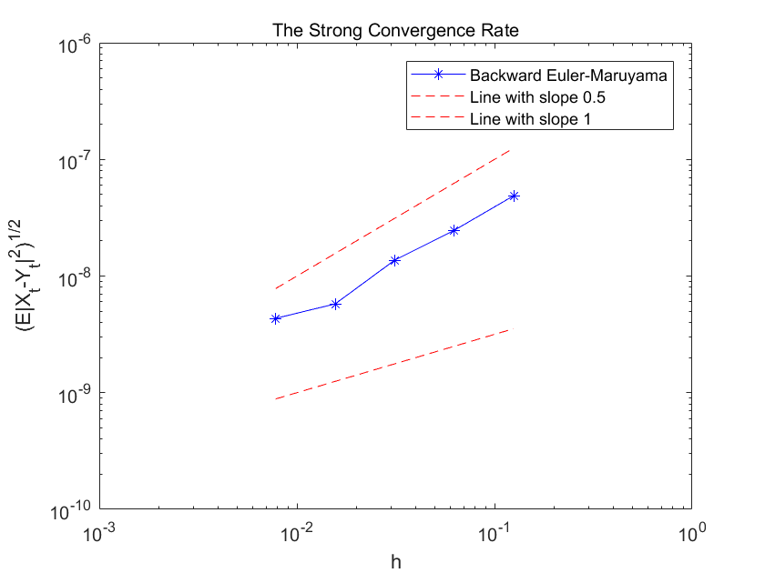
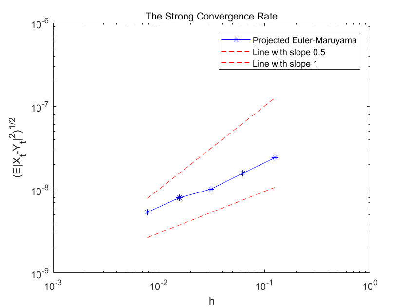
In Figure 1 and Figure 2,
we plot the strong approximation errors of these two numerical schemes for the SDE (5.1).
Set and
use the following time step sizes:
,
where
is considered as the exact solution.
We will use
sample paths to simulate the expectation.
Figure 1: Strong convergence rate of the backward Euler method for
(5.1).
Figure 2: Strong convergence rate of the projected Euler method for
(5.1).
From Figure 1 and Figure 2,
the expected strong convergence rate of order
for both the backward Euler method and
the projected Euler method is numerically confirmed.
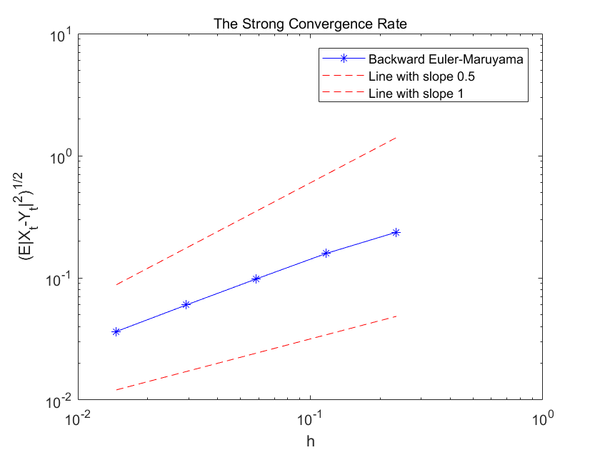
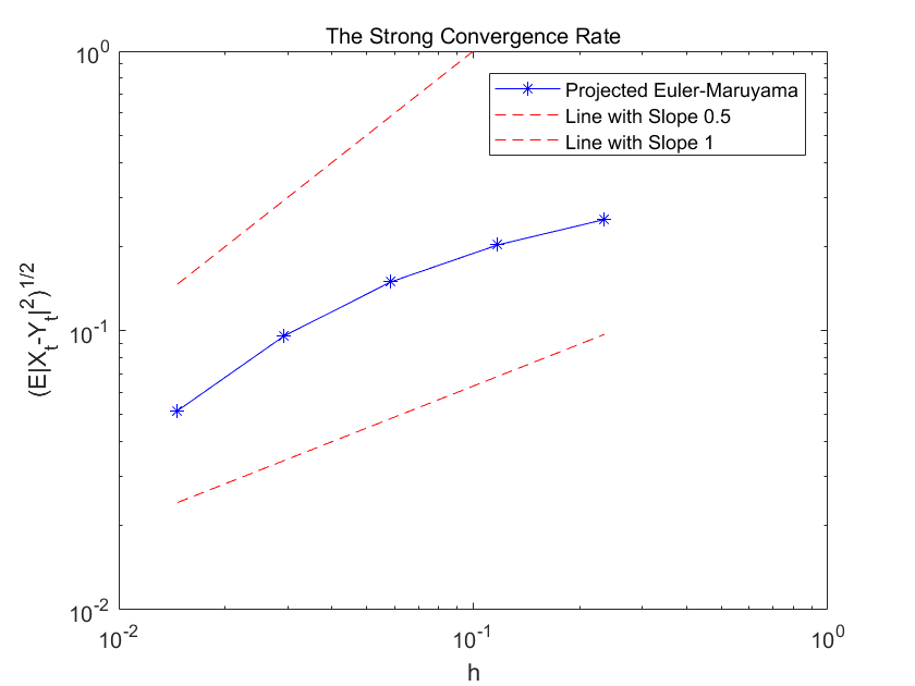
Example 5.2.
Consider the following semi-linear stochastic partial differential equation (SPDE):
(5.2)
where
and
is the real-valued standard Brownian motions.
Such an SPDE is usually termed as the stochastic Allen-Cahn
equation.
We begin by introducing a spatial discretization with a step size
on the interval and denoting the discrete spatial points as
.
The discretization yields an SDE system:
(5.3)
where
,
,
and
Now we turn our attention to the temporal discretization of the SDE system (5.3),
using the backward Euler and projected Euler methods.
For the following numerical tests,
we fix , and
and initialize the system with
.
In Figure 3 and Figure 4,
we plot the strong approximation errors of the two time-stepping schemes for the SDE system (5.3) with .
We use the following time step-sizes:
and the numerical approximation with
is identified as the exact solution.
Moreover, sample paths are used to approximate the expectation.
From Figure 3 and Figure 4,
one can tell the expected strong convergence rate of order
for both the backward Euler method and
the projected Euler method, which confirms the theoretical findings.
Figure 3: Strong convergence rate of
the backward Euler method
for (5.3).
Figure 4: Strong convergence rate of
the projected Euler method
for (5.3).
References
[1]
Adam Andersson and Raphael Kruse.
Mean-square convergence of the BDF2-Maruyama and backward Euler
schemes for SDE satisfying a global monotonicity condition.
BIT Numerical Mathematics, 57(1):21–53, 2017.
[2]
Wolf-Jürgen Beyn, Elena Isaak, and Raphael Kruse.
Stochastic C-stability and B-consistency of explicit and implicit
Euler-type schemes.
Journal of Scientific Computing, 67(3):955–987, 2016.
[3]
Wolf-Jürgen Beyn, Elena Isaak, and Raphael Kruse.
Stochastic C-stability and B-consistency of explicit and implicit
Milstein-type schemes.
Journal of Scientific Computing, 70:1042–1077, 2017.
[4]
Charles-Edouard Brehier.
Approximation of the invariant distribution for a class of ergodic
sdes with one-sided lipschitz continuous drift coefficient using an explicit
tamed euler scheme.
ESAIM: Probability and Statistics, 27:841–866, 2023.
[5]
Nicolas Brosse, Alain Durmus, Éric Moulines, and Sotirios Sabanis.
The tamed unadjusted Langevin algorithm.
Stochastic Processes and their Applications,
129(10):3638–3663, 2019.
[6]
Chuchu Chen, Jialin Hong, and Yulan Lu.
Stochastic differential equation with piecewise continuous
arguments: Markov property, invariant measure and numerical approximation.
Discrete and Continuous Dynamical Systems-B, 28(1):765–807,
2022.
[7]
Arnak S Dalalyan.
Theoretical guarantees for approximate sampling from smooth and
log-concave densities.
Journal of the Royal Statistical Society Series B: Statistical
Methodology, 79(3):651–676, 2017.
[8]
Wei Fang and Michael B Giles.
Adaptive Euler–Maruyama method for SDEs with nonglobally Lipschitz
drift.
The Annals of Applied Probability, 30(2):526–560, 2020.
[9]
Siqing Gan, Youzi He, and Xiaojie Wang.
Tamed Runge-Kutta methods for SDEs with super-linearly growing drift
and diffusion coefficients.
Applied Numerical Mathematics, 152:379–402, 2020.
[10]
Qian Guo, Wei Liu, Xuerong Mao, and Rongxian Yue.
The truncated Milstein method for stochastic differential equations
with commutative noise.
Journal of Computational and Applied Mathematics, 338:298–310,
2018.
[11]
Desmond J Higham, Xuerong Mao, and Andrew M Stuart.
Strong convergence of Euler-type methods for nonlinear stochastic
differential equations.
SIAM journal on numerical analysis, 40(3):1041–1063, 2002.
[12]
Jialin Hong and Xu Wang.
Invariant measures for stochastic nonlinear Schrödinger
equations.
Springer, 2019.
[13]
Martin Hutzenthaler and Arnulf Jentzen.
Numerical approximations of stochastic differential equations
with non-globally Lipschitz continuous coefficients.
American Mathematical Soc., 2015.
[14]
Martin Hutzenthaler and Arnulf Jentzen.
On a perturbation theory and on strong convergence rates for
stochastic ordinary and partial differential equations with nonglobally
monotone coefficients.
The Annals of Probability, 48(1):53–93, 2020.
[15]
Martin Hutzenthaler, Arnulf Jentzen, and Peter E Kloeden.
Strong and weak divergence in finite time of Euler’s method for
stochastic differential equations with non-globally Lipschitz continuous
coefficients.
Proceedings of the Royal Society A: Mathematical, Physical and
Engineering Sciences, 467(2130):1563–1576, 2011.
[16]
Martin Hutzenthaler, Arnulf Jentzen, and Peter E Kloeden.
Strong convergence of an explicit numerical method for SDEs with
nonglobally Lipschitz continuous coefficients.
The Annals of Applied Probability, 22(4):1611–1641, 2012.
[17]
Martin Hutzenthaler, Arnulf Jentzen, and Xiaojie Wang.
Exponential integrability properties of numerical approximation
processes for nonlinear stochastic differential equations.
Mathematics of Computation, 87(311):1353–1413, 2018.
[18]
K Itô and M Nisio.
On stationary solutions of a stochastic differential equation.
J. Math. Kyoto Univ, 4(1):1–75, 1964.
[19]
Cónall Kelly and Gabriel J Lord.
Adaptive time-stepping strategies for nonlinear stochastic systems.
IMA Journal of Numerical Analysis, 38(3):1523–1549, 2018.
[20]
Cónall Kelly, Gabriel J Lord, and Fandi Sun.
Strong convergence of an adaptive time-stepping Milstein method for
SDEs with monotone coefficients.
BIT Numerical Mathematics, 63(2):33, 2023.
[21]
Peter E Kloeden and Eckhard Platen.
Numerical Solution of Stochastic differential equations.
Springer, 1992.
[22]
Ruilin Li, Hongyuan Zha, and Molei Tao.
Sqrt (d) dimension dependence of Langevin Monte Carlo.
ICLR, 2022.
[23]
Xiaoyue Li, Xuerong Mao, and George Yin.
Explicit numerical approximations for stochastic differential
equations in finite and infinite horizons: truncation methods, convergence in
pth moment and stability.
IMA Journal of Numerical Analysis, 39(2):847–892, 2019.
[24]
Wei Liu, Xuerong Mao, and Yue Wu.
The backward Euler-Maruyama method for invariant measures of
stochastic differential equations with super-linear coefficients.
Applied Numerical Mathematics, 184:137–150, 2023.
[25]
Wei Liu and Yudong Wang.
Strong convergence in the infinite horizon of numerical methods for
stochastic differential equations.
arXiv preprint arXiv:2307.05039, 2023.
[26]
Xuerong Mao.
Stochastic differential equations and applications.
Elsevier, 2007.
[27]
Xuerong Mao.
The truncated Euler–Maruyama method for stochastic differential
equations.
Journal of Computational and Applied Mathematics, 290:370–384,
2015.
[28]
Xuerong Mao and Lukasz Szpruch.
Strong convergence and stability of implicit numerical methods for
stochastic differential equations with non-globally Lipschitz continuous
coefficients.
Journal of Computational and Applied Mathematics, 238:14–28,
2013.
[29]
Xuerong Mao and Lukasz Szpruch.
Strong convergence rates for backward Euler–Maruyama method for
non-linear dissipative-type stochastic differential equations with
super-linear diffusion coefficients.
Stochastics An International Journal of Probability and
Stochastic Processes, 85(1):144–171, 2013.
[30]
Jonathan C Mattingly, Andrew M Stuart, and Desmond J Higham.
Ergodicity for SDEs and approximations: locally Lipschitz vector
fields and degenerate noise.
Stochastic processes and their applications, 101(2):185–232,
2002.
[31]
Jonathan C Mattingly, Andrew M Stuart, and Michael V Tretyakov.
Convergence of numerical time-averaging and stationary measures via
Poisson equations.
SIAM Journal on Numerical Analysis, 48(2):552–577, 2010.
[32]
Grigori N Milstein and Michael V Tretyakov.
Stochastic numerics for mathematical physics, volume 39.
Springer, 2004.
[33]
Andreas Neuenkirch and Lukasz Szpruch.
First order strong approximations of scalar sdes defined in a domain.
Numerische Mathematik, 128:103–136, 2014.
[34]
Chenxu Pang, Xiaojie Wang, and Yue Wu.
Linear implicit approximations of invariant measures of semi-linear
sdes with non-globally lipschitz coefficients.
Journal of Complexity, 83:101842, 2024.
[35]
Sotirios Sabanis.
Euler approximations with varying coefficients: the case of
superlinearly growing diffusion coefficients.
Annals of Applied Probability, 26(4):2083–2105, 2016.
[36]
Yang Song, Jascha Sohl-Dickstein, Diederik P Kingma, Abhishek Kumar, Stefano
Ermon, and Ben Poole.
Score-based generative modeling through stochastic differential
equations.
In the 9th International Conference on Learning Representations
(ICLR), 2021.
[37]
Denis Talay.
Second-order discretization schemes of stochastic differential
systems for the computation of the invariant law.
Stochastics: An International Journal of Probability and
Stochastic Processes, 29(1):13–36, 1990.
[38]
Denis Talay.
Stochastic Hamiltonian systems: exponential convergence to the
invariant measure, and discretization by the implicit Euler scheme.
Markov Process. Related Fields, 8(2):163–198, 2002.
[39]
Michael V Tretyakov and Zhongqiang Zhang.
A fundamental mean-square convergence theorem for SDEs with locally
Lipschitz coefficients and its applications.
SIAM Journal on Numerical Analysis, 51(6):3135–3162, 2013.
[40]
Xiaojie Wang.
Mean-square convergence rates of implicit Milstein type methods for
SDEs with non-Lipschitz coefficients.
Advances in Computational Mathematics, 49(3):37, 2023.
[41]
Xiaojie Wang and Siqing Gan.
The tamed Milstein method for commutative stochastic differential
equations with non-globally Lipschitz continuous coefficients.
Journal of Difference Equations and Applications,
19(3):466–490, 2013.
[42]
Xiaojie Wang, Jiayi Wu, and Bozhang Dong.
Mean-square convergence rates of stochastic theta methods for SDEs
under a coupled monotonicity condition.
BIT Numerical Mathematics, 60(3):759–790, 2020.
[43]
Max Welling and Yee W Teh.
Bayesian learning via stochastic gradient Langevin dynamics.
In Proceedings of the 28th international conference on machine
learning (ICML-11), pages 681–688. Citeseer, 2011.
Appendix A Appendix
Proof of Theorem
2.5.
To highlight the dependence on initialization, we denote the solution of an SDE as
.
Now,
consider the error of the method
at the -step
(A.1)
It is apparent that the primary distinction on the right-hand side of equation
(A.1)
arises from the difference on the initial data at time ,
resulting in errors in the solution at the th step.
This can be reformulated as:
(A.2)
where is given by (2.21).
The second difference in equality
(A.1)
is the one-step error at the
-step and we denote it as
(A.3)
Let be an integer.
We have
(A.4)
where only depends on .
For the first term on the right-hand side of
(A.4),
by (2.22)
we have
(A.5)
Next,
we perform a further decomposition of the second term
on the right-hand side of (A.4)
as follows:
(A.6)
Due to the
-measurability of
and the conditional variant of
(2.30),
we obtain for the first term on the right-hand side of
(A.6),
(A.7)
For the second term on the right-hand side of
(A.6),
noting that it equals zero when ,
we have for ,
(A.8)
where only depends on .
Additionally,
one can utilize -measurability
of and the conditional variants of
(2.31),
(2.22) and (2.23),
along with the Hölder inequality,
to derive for ,
(A.9)
where depend on ,
and .
Moreover,
one can bound the third term on the right-hand side of
(A.6),
by employing the conditional variants of
(2.31),
(2.22),
(2.23),
along with applying the Hölder inequality (twice):
(A.10)
where depends on .
Following the conditional versions of
(2.31)
and (2.22)
as well as the Hölder inequality,
one can bound the third third term on the right-hand side of the inequality (A.4) as follows:
(A.11)
where depends on
.
By Substituting the inequalities
(A.5) to
(A.11)
into
(A.4)
and recalling that
,
one can obtain
(A.12)
Then using the Young inequality for
(A.12),
we have
(A.13)
where is independent of .
Given the assumption that
and the inequality
for ,
we can proceed by utilizing the inequalities
,
(2.12) and
(2.32) and obtain
(A.14)
where
Equipped with the above inequality,
one sees
(A.15)
where the constant does not depend on .
Namely,
(A.16)
To conclude,
Theorem 2.5 is proved for integer .
For non-integer , the conclusion can be derived using the Young inequality. Therefore,
the proof is completed.