Optimization-based Structural Pruning for Large Language Models without Back-Propagation

Abstract

Compared to the moderate size of neural network models, structural weight pruning on the Large-Language Models (LLMs) imposes a novel challenge on the efficiency of the pruning algorithms, due to the heavy computation/memory demands of the LLMs. Recent efficient LLM pruning methods typically operate at the post-training phase without the expensive weight finetuning, however, their pruning criteria often rely on heuristically designed metrics, potentially leading to suboptimal performance. We instead propose a novel optimization-based structural pruning that learns the pruning masks in a probabilistic space directly by optimizing the loss of the pruned model. To preserve the efficiency, our method 1) works at post-training phase and 2) eliminates the back-propagation through the LLM per se during the optimization (i.e., only requires the forward pass of the LLM). We achieve this by learning an underlying Bernoulli distribution to sample binary pruning masks, where we decouple the Bernoulli parameters from the LLM loss, thus facilitating an efficient optimization via a policy gradient estimator without back-propagation. As a result, our method is able to 1) operate at structural granularities of channels, heads, and layers, 2) support global and heterogeneous pruning (i.e., our method automatically determines different redundancy for different layers), and 3) optionally use a metric-based method as initialization (of our Bernoulli distributions). Extensive experiments on LLaMA, LLaMA-2, and Vicuna using the C4 and WikiText2 datasets demonstrate that our method operates for 2.7 hours with around 35GB memory for the 13B models on a single A100 GPU, and our pruned models outperform the state-of-the-arts w.r.t. perplexity. Codes will be released.

1 Introduction

With the rapid development of Large Language Models [7, 1] (LLMs) and their expanding multitude of applications across various domains, the efficiency of LLMs with vast parameters and complex architectures becomes crucial for practical deployment. In this paper, we aim to compress the LLM through structural pruning, which removes certain structural components such as channels or layers to reduce the model size with hardware-friendly acceleration.

Pioneering structural pruning in the pre-LLM era involves pruning channels or layers through optimization, which determines the structures to prune by back-propagating the task loss through the networks [34, 5, 66, 35, 17, 15]. These methods operate at the in-training [25, 14, 65, 23] or post-training [40, 50, 32] phase, where the latter exhibit better efficiency without model weights update. In the following, we focus on discussing post-training pruning to ensure efficiency.

However, the heavy computational and memory demands of LLMs make existing optimization-based methods less appropriate for LLM pruning in terms of efficiency. Metric-based pruning is introduced to alleviate this issue, which directly prunes specific network components based on carefully designed criteria, such as the importance score [46, 12]. Nonetheless, those criteria are often based on heuristics, which potentially impede the performance of the pruned models and can thus be further optimized to achieve a better local minimum. As a result, metric-based pruning methods may face challenges in achieving promising performance and generalizability, particularly when the pruning rate is high.

for tree= edge path= [edge](!u.parent anchor) – +(5pt,0) |- (.child anchor)edge label;, grow=0, reversed, parent anchor=east, child anchor=west, anchor=west, [LLM Pruning Methods, root [ w/ Weight Update [Metric-based [Only Forward, l sep=8mm, [ Structured: [2, 49, 57]
Unstructured: [6, 16, 49, 60, 62], tnode] ] [Need Backward, l sep=5.25mm, [ Structured: [9, 52, 61]
Unstructured: N/A, tnode] ] ] [Optim-based [Only Forward, l sep=8.4mm, [N/A (Cannot Update Weights), tnode] ] [Need Backward, l sep=5.7mm, [ Structured: [8, 20, 28, 30, 64, 55]
Unstructured: N/A, tnode] ] ] ] [w/o Weight Update [Metric-based [Only Forward, l sep=6.35mm, [$\spadesuit$ Structured: [2, 3, 27]
Unstructured: [31, 44, 46, 56, 58, 63], tnode] ] [Need Backward, l sep=3.55mm, [$\spadesuit$ Structured: [36]
Unstructured: [12], tnode] ] ] [Optim-based [Only Forward, l sep=6.75mm, [ Structured: Our Method
Unstructured: N/A, tnode] ] [Need Backward, l sep=4mm, [N/A (Less Efficient), tnode] ] ] ] ]

Figure 1: The taxonomy of our method among the LLM Pruning. Methods without weight update are used for comparison in our experiments (highlighted with $\spadesuit$), due to the constraints on time and memory efficiency, as well as the accessibility of large-scale finetuning datasets.

Moreover, the majority of metric-based methods typically prune the networks by manually-designed thresholds [31, 63]. Although different layers of LLMs may have varying levels of redundancy [58, 56], achieving a global and heterogeneous pruning strategy is challenging with metric-based approaches. This arises due to the significantly varying magnitudes of the manually designed metrics across layers, making it laborious or even impossible to set proper pruning threshold for each layer.

In view of those limitations, we propose a lightweight optimization-based method to ensure performance with global and heterogeneous pruning, which can be optionally initialized by an arbitrary metric-based approach. Our pruning efficiency is achieved using a policy gradient estimator [53], which only requires the LLM forward pass (i.e., being analogous to many efficient metric-based methods with the same memory requirement, such as [44, 38, 16, 2]), and avoids the heavy gradients back-propagation through the LLM. Moreover, our method unifies the pruning of the entire LLM into a probabilistic space, eliminating the magnitude difference issue of most metric-based methods, therefore directly facilitating global and heterogeneous pruning across the entire LLM.

Specifically, we formulate our pruning as a binary mask learning problem, where the binary masks determine whether to retain or prune the corresponding structures by element-product of them. To efficiently learn those binary masks, we construct an underlying probabilistic space of Bernoulli distributions, which is used to sample the binary masks. As we decouple the Bernoulli parameters and the sampled makes, resulting in a disentanglement of the Bernoulli parameters from the LLM loss, our method can thus be optimized in a back-propagation-free manner (regarding the heavy LLMs) efficiently exploiting the policy gradient estimator. Moreover, the probabilistic modeling of Bernoulli distribution facilitates global and heterogeneous pruning across the entire LLM. Furthermore, by formulating the masks at the different structural granularities, our method supports pruning at channels, heads (of multi-head attention modules), and layers.

The taxonomy of our methods is illustrated in Fig. 1, our method is compared with state-of-the-art structural pruning methods that do not involve model weight updates, due to the constraints on time and memory efficiency, as well as the accessibility of large-scale finetuning datasets. We extensively validate our methods using the C4 [41] and WikiText2 [39] datasets on popular LLaMA [47], LLaMA-2 [48], and Vicuna [10] models with 7B and 13B parameter sizes, 30% to 50% pruning rates, and various initialization. Those demonstrate that our method operates for 2.7 hours with about 35GB memory on a single A100 GPU, which outperforms the state-of-the-art w.r.t. perplexity. Our method exhibits the following features simultaneously:

• Accuracy with large pruning rates for LLMs, ensured by 1) our optimization-based pruning without heuristically designed metrics, which can optionally take metric-based pruning as initialization for a better convergence, and 2) the global and heterogeneous pruning, as supported by our probabilistic modeling of the pruning masks.

• Efficiency for both computations and memory, achieved by the policy gradient estimator, facilitating back-propagation-free and forward-only optimization w.r.t. the heavy LLMs.

• Flexibility across various structural pruning granularities including channels, heads, and layers, coming from our mask formulation of pruning that can be inherently applied to different structural granularities.

2 Related Work

Pruning has proven effective in traditional deep neural networks [21, 15, 29, 19], and extensive research has been conducted on this topic. Typically, post-pruning performance is restored or even enhanced through full-parameter fine-tuning [34, 5]. However, for large language models (LLMs) with their vast number of parameters, full-parameter fine-tuning is computationally expensive and often impractical. To overcome this challenge, various pruning strategies [28, 54, 26, 61, 8, 64, 3, 13, 38] have been developed for LLMs in recent years. These strategies can be categorized into metric-based pruning and optimization-based pruning.

Metric-based Pruning. Metric-based pruning methods focus on designing importance metrics for model weights or modules. The most representative method is Wanda [46]. It introduces a simple but effective pruning metric by considering both the magnitude of weights and activations without updating model parameters. LLM-Pruner [36] efficiently trims LLMs by pinpointing and eliminating non-essential coupled structures, assessing weight importance via loss change, and using Taylor expansion to preserve performance. SparseGPT [16] adapts the OBS [22] by an efficient technique for estimating the Hessian matrix to reconstruct the model. These methods use pre-defined pruning metrics and often fail to perform well at high sparsity levels. Additionally, updating the model parameters to maintain performance after pruning requires more computational resources. Our method automatically achieves optimal pruning results through an optimized approach, without the need for weight updates, significantly reducing computational load.

Optimization-based Pruning. Optimization-based pruning methods focus on determining the model mask in an optimized manner and also involve updating the model parameters. Sheared LLaMA [55] learns pruning masks to find a subnetwork that fits a target architecture and maximizes performance, utilizing dynamic batch loading for efficient data usage. Compresso [20] optimizes LLM pruning by integrating LoRA [24] with L0 regularization and dynamically updates parameters during instruction tuning to enhance post-pruning performance and adaptability. LoRAShear [8] and APT [64] also utilize LoRA in the pruning process alongside weight updating. However, these methods, including the optimization process and weight finetuning, invariably rely on back-propagation, which is time and memory-intensive. We propose using policy gradient estimation in the optimization process as an alternative to back-propagation, which significantly conserves computational resources.

3 Methodology

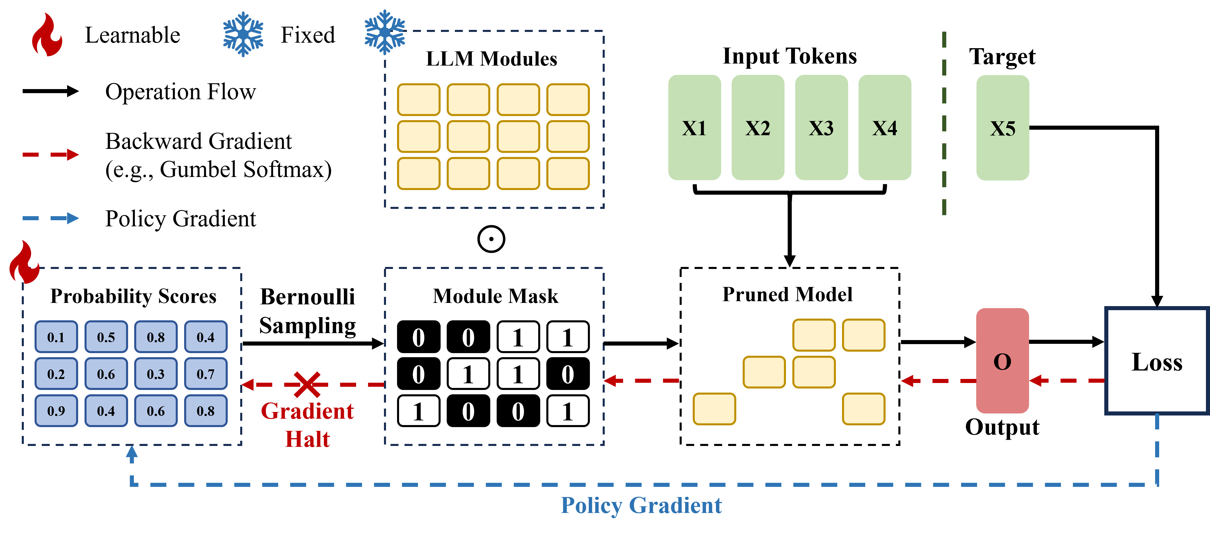
Figure 2: The overview of our method. We formulate LLM pruning as optimizing underlying Bernoulli distributions that sample binary masks. Being different from the conventional back-propagation method (e.g., through Gumbel Softmax as shown by the red-dashed-arrows), our formulation decouples the masks and the Bernoulli parameters from the LLM loss (see Eq. (4) and Remark 3), facilitating efficient and unbiased policy gradient (the blue-dashed-arrow) without back-propagation through the LLM (see Eq. (5) and Remark 4). $\odot$ denotes element-wise product.

We introduce our optimization-based pruning for LLMs, which is efficient without back-propagation through the LLM. We detail our probabilistic mask modeling in Sect. 3.1, and our optimization via policy gradient estimator in Sect. 3.2. The overview of our method is illustrated in Fig. 2.

3.1 Pruning via Probabilistic Mask Modeling

We formulate the network pruning as seeking binary masks to determine whether the corresponding structure should be pruned or retrained. Those binary masks are further modeled by/sampled from underlying Bernoulli distributions stochastically. Such formulation possesses several merits: 1) the mask formulation enables flexible pruning at channels, heads (of Multi-Head Attention, MHA), and layers; 2) the probabilistic Bernoulli modeling facilitates global and heterogeneous pruning across the entire LLM; and 3) the stochastical sampling decouples Bernoulli parameters and masks from LLM loss thus empowers a efficient policy gradient optimization without back-propagate through the LLM (see Sect. 3.2).

Specifically, denoting the calibration dataset with $N$ i.i.d. samples as $\mathcal{D}=\{(\mathbf{x}_{i},\mathbf{y}_{i})\}^{N}_{i=1}$, $\mathbf{w}=\{\mathbf{w}_{i}\}^{n}_{i=1}$ as the complete and non-overlapped modules of a LLM with model size $n$, and $\mathbf{m}=\{\mathbf{m}_{i}\}^{n}_{i=1}\in\{0,1\}^{n}$ as the corresponding binary masks, where $\mathbf{m}_{i}=0$ implies $\mathbf{w}_{i}$ is pruned and otherwise $\mathbf{w}_{i}$ is retained. We note that $\mathbf{w}_{i}$ and $\mathbf{m}_{i}$ can be defined with various granularities such as channels, heads, and layers for structural pruning. Then, our structural pruning of LLMs can be formulated as a binary optimization with constraints:

$$\min_{\mathbf{m}}\ \mathcal{L}(\mathcal{D};\mathbf{w} \odot\mathbf{m}):=\frac{1}{N}\sum_{i=1}^{N}\ell(f(\mathbf{x}_{i};\mathbf{w}\odot\mathbf{m}),\mathbf{y}_{i}),$$ (1)

s.t. $$\left\|\mathbf{m}\right\|_{1}\leq rn\ \text{ and }\ \mathbf{m}\in\{0,1\}^{n}.$$

where $f(\cdot;\mathbf{w}\odot\mathbf{m})$ is the pruned network, $\ell(\cdot,\cdot)$ is the loss function, e.g., the cross-entropy loss, and $r$ is the target pruning rate. We note that the binary optimization problem in Eq. (1), i.e., finding high quality masks $\mathbf{m}$ from the discrete and exponentially growing solution space, is typically NP-hard.

Therefore, we relax the discrete optimization using a probabilistic approach, by treating $n$ masks as binary random variables sampled from $n$ underlying Bernoulli distributions with parameters $\mathbf{s}=\{\mathbf{s}_{i}\}^{n}_{i=1}\in[0,1]^{n}$. This yields the conditional distribution of m over $\mathbf{s}$:

$$p(\mathbf{m}|\mathbf{s})=\prod_{i=1}^{n}(s_{i})^{m_{i}}(1-s_{i})^{1-m_{i}}.$$ (2)

By relaxing the $\ell_{1}$ norm in Eq. (1) using its expectation, i.e., $\mathbb{E}_{\mathbf{m}\sim p(\mathbf{m}|\mathbf{s})}\left\|\mathbf{m}\right\|_{1}=\sum_{i=1}^{n}s_{i}=\mathbf{1}^{\top}\mathbf{s}$, we have the following excepted loss minimization problem:

$$\min_{\mathbf{s}} \mathbb{E}_{p(\mathbf{m}|\mathbf{s})}\mathcal{L}(\mathcal{D};\mathbf{w}\odot\mathbf{m}),$$ (3)

$$\text{s.t.}\ \mathbf{1}^{\top} \mathbf{s}\leq rn\ \text{ and }\ \mathbf{s}\in[0,1]^{n}.$$

Remark 1

Problem (3) is a continuous relaxation of the discrete Problem (1). The feasible region of Problem (3) is as simple as the intersection of the cube $[0,1]^{n}$ and the half-space $\mathbf{1}^{\top}\mathbf{s}\leq rn$. Moreover, the parameterization of Problem (3) in the probabilistic space facilitates automatically learning the redundancy across different layers for global and heterogeneous pruning.

3.2 Optimization by Policy Gradient Estimator

Conventional neural network training paradigm usually adopts back-propagation to estimate the gradient of Eq. (3), e.g., through the Gumbel-Softmax trick [37]. In order to flow the gradients, such methods typically reparameterize the mask $\mathbf{m}$ as a function of $\mathbf{s}$, i.e., $m_{i}=\phi(s_{i})$ or $m_{i}=\phi(s_{i},\epsilon)$ with $\epsilon\sim\mathcal{N}(0,1)$. However, the back-propagation has the following intrinsic issues in LLM pruning.

Remark 2

Intrinsic issues of back-propagation in LLM pruning: 1) the back-propagation is computationally expensive and would also cost a large amount of memory; 2) the computation of gradients can not be satisfied by using the sparsity in $\mathbf{m}$, i.e., $\frac{\partial m_{i}}{\partial s_{i}}\neq 0$ even if $m_{i}=0$. In other words, one has to go through the full model for back-propagation even when lots of the modules in LLM have been masked; 3) the widely used Gumbel-Softmax is known to be biased [37].

Now we present our efficient (back-propagation-free) and unbiased optimization for Problem (3). We proposed to adopt Policy Gradient Estimator (PGE) to estimate the gradient with only forward propagation, avoiding the pathology of the chain-rule-based estimator. Specifically, in order to update the Bernoulli parameters $\mathbf{s}$, we have the following objective:

$$\Phi(\mathbf{s})=\mathbb{E}_{p(\mathbf{m}|\mathbf{s})}\mathcal{L}(\mathcal{D};\mathbf{w}\odot\mathbf{m}) =\int p(\mathbf{m}|\mathbf{s})\mathcal{L}(\mathcal{D};\mathbf{w}\odot\mathbf{m})\text{d}\mathbf{m},$$ (4)

$$\text{s.t.}\ \mathbf{1}^{\top}\mathbf{s}\leq rn \ \text{ and }\ \mathbf{s}\in[0,1]^{n}.$$

Remark 3

Our key idea is that in Eq. (4), the score vector $\mathbf{s}$ only appears in the conditional probability for sampling $\mathbf{m}$, which is not composited into the network loss term $\mathcal{L}(\mathcal{D};\mathbf{w}\odot\mathbf{m})$. In other words, being different from the Gumbel-Softmax estimator where $\mathbf{m}$ is a function of $\mathbf{s}$, we formulate $\mathbf{m}$ as a random variable which is only related to $\mathbf{s}$ through the conditional probability of probabilistic sampling. Therefore, the expensive back-propagation through the LLM can be omitted in gradient estimation using the PGE.

Specifically, the optimization of Eq. (4) via the policy gradient estimator holds that:

$$\nabla_{\mathbf{s}}\Phi(\mathbf{s}) =\int\mathcal{L}(\mathbf{m})\nabla_{\mathbf{s}}p(\mathbf{m}|\mathbf{s})+\underbrace{p(\mathbf{m}|\mathbf{s})\nabla_{\mathbf{s}}\mathcal{L}(\mathbf{m})}_{=\ 0}\text{d}\mathbf{m}$$ (5)

$$=\int\mathcal{L}(\mathbf{m})p(\mathbf{m}|\mathbf{s})\nabla_{\mathbf{s}}\log(p(\mathbf{m}|\mathbf{s}))\text{d}\mathbf{m}$$

$$=\mathbb{E}_{p(\mathbf{m}|\mathbf{s})}\mathcal{L}(\mathbf{m})\nabla_{\mathbf{s}}\log(p(\mathbf{m}|\mathbf{s})).$$

The last equality demonstrates that $\mathcal{L}(\mathbf{m})\nabla_{\mathbf{s}}\log(p(\mathbf{m}|\mathbf{s}))$ is an unbiased stochastic gradient for $\Phi(\mathbf{s})$.

Remark 4

The efficiency of Eq. (5): 1) Equation (5) can be computed with purely forward propagation, 2) the computation can be fully sparsfied by exploiting the sparsity in $\mathbf{m}$, 3) the computation cost for the gradients, i.e., $\nabla_{\mathbf{s}}\log(p(\mathbf{m}|\mathbf{s}))=\frac{\mathbf{m}-\mathbf{s}}{\mathbf{s}(1-\mathbf{s})}$, is negligible. Therefore, our PGE is computationally efficient compared to the backward-propagation-based estimators.

The stochastic gradient descent algorithm in the batch-training paradigm is:

$$\mathbf{s}\leftarrow\textbf{proj}_{\mathcal{C}}(\mathbf{z})\ \text{with}\ \mathbf{z}:=\mathbf{s}-\eta\mathcal{L}(\mathcal{D}_{B};\mathbf{w}\odot\mathbf{m})\nabla_{\mathbf{s}}\log(p(\mathbf{m}|\mathbf{s})).$$ (6)

where $\mathcal{D}_{B}=\{(\mathbf{x}_{i},\mathbf{y}_{i})\}^{B}_{i=1}$ is batch samples from $\mathcal{D}$ with batch size $B$, and $\mathcal{L}(\mathcal{D}_{B};\mathbf{w}\odot\mathbf{m})$ is the loss on $\mathcal{D}_{B}$ with the pruned model by masks $\mathbf{m}$. The projection operator $\textbf{proj}_{\mathcal{C}}(\cdot)$ is to ensure the updated scores $\mathbf{s}$ to be constrained in the feasible domain $\mathcal{C}$ that satisfies $\mathcal{C}=\left\{\mathbf{1}^{\top}\mathbf{s}\leq K\right\}\bigcap\left\{\mathbf{s}\in[0,1]^{n}\right\}$. We implement the projection operator from [51], the details of which can be found in Appendix A.

Policy gradient is known to be impeded by its large variance [33]. In order to reduce the variance and improve the stability of training, we minus a moving average baseline which is calculated by 1) firstly obtaining the averaged loss of multiple mask sampling trials, then 2) taking the moving average of the current averaged and the previous losses with a window size. Denote the baseline as $\delta$, given window size $T$ (set to 5), and mask sampling times $N_{s}$ (set to 2), we update $\mathbf{s}$ in each training step via:

$$\mathbf{s}\leftarrow\textbf{proj}_{\mathcal{C}}(\mathbf{z})\ \text{with}\ \mathbf{z} :=\mathbf{s}-\eta[\frac{1}{N_{s}}\sum_{i=1}^{N_{s}}(\mathcal{L}(\mathcal{D}_{B};\mathbf{w}\odot\mathbf{m}^{(i)}){\color[rgb]{1,0,0}-\delta})\nabla_{\mathbf{s}}\log(p(\mathbf{m}^{(i)}|\mathbf{s}))\ ].$$ (7)

$$\delta \leftarrow\frac{T-1}{T}\delta+\frac{1}{N_{s}T}\sum_{i=1}^{N_{s}}\mathcal{L}(\mathcal{D}_{B};\mathbf{w}\odot\mathbf{m}^{(i)}).$$ (8)

Our efficient pruning algorithm is summarized in Appendix A. Note that our formulation can also be interpreted from a dense rewards reinforcement learning perspective, as discussed in Appendix B.

Initialization. Algorithms based on policy gradient usually require an effective initialization to get enhanced results. In this context, previous hand-crafted pruning metric can be applied to initialize the probability of each module: $\mathbf{s}_{0}\leftarrow\sigma(\mathbf{x})$, in which $\mathbf{x}$ is any pruning metric derived from existing method, $\mathbf{s}_{0}$ represents the initial probability assigned to each module, and $\sigma$ symbolizes a non-linear transformation. We extensively discuss different initializations $\mathbf{x}$ (including a random strategy with good performance) in Appendix C, and different transformations $\sigma$ in Appendix D.

Applicability of PGE in Learning Pruning Masks. We note that the precision of PGE may not match that of conventional back-propagation. Given that we are learning the binary masks $\mathbf{m}$ (distinct from the float weights), it is expected that the precision requirement of $\mathbf{s}$ can be modest. Moreover, our PGE is unbiased (compared to the biased Gumbel Softmax). These factors make the PGE suitable for learning the pruning masks, which is empirically validated with extensive experiments.

4 Experiments

Extensive experiments have been conducted in this section to validate the promising performance of the proposed method. In short, our method has been validated across different LLM models with various sizes, pruning rates, structural granularities for pruning (i.e., channels, heads, and layers), and initializations (in the ablation analysis). In the following, we first detail our experimental setups in Sect. 4.1. After that, our main results against the state-of-the-art methods for channels and heads pruning, as well as layers pruning, are shown in Sects. 4.2 and 4.3, respectively. Our method runs 2.7 hours for LLaMA-2-13B with a similar GPU memory (i.e., $\sim$35GB) as Wanda-sp [2], details are shown in Appendix H. We also show multiple-runs statistics of our method in Appendix I.

4.1 Experimental Setups

Structural Granularities for Pruning. We validate our method on various structural granularities for pruning, namely channels, heads, and layers. We detail the settings of the granularities and the initializations, as well as the state-of-the-art methods for comparison in the following. In short, Methods without weight update are used for comparison, due to the constraints on time and memory efficiency, as well as the accessibility of large-scale finetuning datasets. For the effects of different initializations, we extensively investigated them in Sect. 5 and Appendices C and D.

Specifically, we follow [36, 61] to prune the heads of the multi-head attention (MHA) modules and the channels of the multi-layer perceptron (MLP) modules in Sect. 4.2. In this experiment, we initialize our methods with an efficient metric-based structural pruning method, i.e., Wanda-sp [2]. Our method is compared to the state-of-the-art Wanda-sp [2], LLM-Pruner [36], and SliceGPT [16].

Beyond that, we also validate the layer pruning, where we prune the entire transformer layer consisting of an MHA module and an MLP module. Note that pruning on the structural granularity of layers is less exploited for LLMs, thus in this experiment, we use the lightweight Layerwise-PPL [27] for initialization, and compare our method with Layerwise-PPL [27].

LLM Models and Sizes. LLaMA-{7B, 13B} [47], LLaMA-2-{7B, 13B} [48], and Vicuna1.3-{7B, 13B} [10] are used as the source models to prune throughout all of our experiments.

Pruning Rate. Promising performance with a high pruning rate could be challenging to obtain when employing metric-based pruning, owing to the heuristically designed metrics. To validate the superior performance of our optimization-based pruning under this situation, we select high pruning rates ranging from 30% to 50%, i.e., structurally removing 30% to 50% model parameters.

Datasets. We perform the experiments following the cross-dataset settings in [46], where the C4 dataset [41] is used for training and the WikiText2 dataset [39] is used for evaluation. This challenging cross-dataset setup potentially better reflects the generalization of the pruned model.

Training and Evaluation Details. We update the underlying Bernoulli distributions (for mask sampling) simply using stochastic gradient descent with a learning rate of 2e-3 for all our experiments. The batch size is fixed to 8 and we train our lightweight policy gradient estimator for 1 epoch on the C4 dataset with 120K segments, in which each segment has a sequence length of 128. To carry out a fair comparison, the network weights are fixed for all the models without retraining/funtuning.

To reduce the evaluation variance, we deterministically generate the pruned evaluation architecture, i.e., given a prune rate $r$, we first rank all the $\mathbf{s}$, then deterministically set $\mathbf{m}$ corresponding to the minimal $r$ of $\mathbf{s}$ as 0 (otherwise 1). We report the perplexity on the WikiText2 dataset using a sequence length of 128. Given a tokenized sequence $\mathbf{X}=(x_{0},x_{1},\dots,x_{t})$, the perplexity of $\mathbf{X}$ is:

$$\text{Perplexity}(\mathbf{X})=\text{exp}\left\{-\frac{1}{t}\sum_{i}^{t}\log p_{\theta}(x_{i}|x_{<i})\right\},$$

where $\log p_{\theta}(x_{i}|x_{<i})$ is the log-likelihood of token $x_{i}$ conditioned on the preceding tokens $x_{<i}$.

4.2 Results on Channels and Heads Pruning

The results of channels and heads pruning following [36, 61] are shown in Table 1 and Table A3 of Appendix E. Our method achieves the lowest perplexity scores among the SOTA methods, given its initialization of Wanda-sp does not perform as well as SOTAs. It demonstrates the superiority of optimization-based global and heterogeneous pruning. Especially, such outperformance is more significant at larger pruning rates over 40%.

Table 1: Results on channels and heads pruning. Our method is initialized by Wanda-sp (please also refer to Sect. 5.1 and Appendix C for a detailed discussion about initializations). All the methods are calibrated using the C4 dataset and validated on the WikiText2 dataset w.r.t. perplexity.

Method	PruneRate	LLaMA		LLaMA-2		Vicuna
		7B	13B	7B	13B	7B	13B
Dense	0$\%$	12.62	10.81	12.19	10.98	16.24	13.50
LLM-Pruner	30$\%$	38.41	24.56	38.94	25.54	48.46	31.29
SliceGPT		-	-	40.40	30.38	52.23	57.75
Wanda-sp		98.24	25.62	49.13	41.57	57.60	80.74
Ours		25.61	19.70	28.18	21.99	34.51	26.42
LLM-Pruner	40$\%$	72.61	36.22	68.48	37.89	88.96	46.88
SliceGPT		-	-	73.76	52.31	89.79	130.86
Wanda-sp		110.10	165.43	78.45	162.50	85.51	264.22
Ours		42.96	28.12	39.81	31.52	51.86	43.59
LLM-Pruner	50$\%$	147.83	67.94	190.56	72.89	195.85	91.07
SliceGPT		-	-	136.33	87.27	160.04	279.33
Wanda-sp		446.91	406.60	206.94	183.75	242.41	373.95
Ours		72.02	49.08	65.21	52.23	71.18	68.13

4.3 Results on Layer Pruning

We illustrate the results on layer pruning in Tables 2 and Table A4 of Appendix E, which demonstrate that our method significantly outperforms the baseline method with pruning rates larger than 40%. For LLaMA-13B and LLaMA-2-13B with moderate pruning rates of 30% and 35%, our method works comparable with Layerwise-PPL, which might imply that the searching space for optimization is too small with a coarse pruning granularity of layer, and the larger 13B models have more redundancy thus works well with metric-based pruning with 30% and 35% pruning rates.

Table 2: Results on layers pruning. Our method is initialized by Layerwise-PPL (please also refer to Sect. 5.1 and Appendix C for detailed discussion about initializations). All the methods are calibrated using the C4 dataset and validated on the WikiText2 dataset w.r.t. perplexity.

Method	PruneRate	LLaMA		LLaMA-2		Vicuna
		7B	13B	7B	13B	7B	13B
Dense	0$\%$	12.62	10.81	12.19	10.98	16.24	13.50
Layerwise-PPL	30$\%$	31.65	24.23	24.83	20.52	37.99	29.85
Ours		24.45	24.44	23.20	21.93	29.16	24.68
Layerwise-PPL	40$\%$	54.97	50.57	41.45	32.48	64.96	54.12
Ours		42.73	39.07	38.26	30.99	54.37	35.73
Layerwise-PPL	50$\%$	107.12	183.93	126.08	78.04	517.46	153.53
Ours		94.97	66.38	104.37	69.92	126.24	84.90

5 Ablation Analysis

In this section, we investigate 1) effect of different initialization of our method in Sect. 5.1 and Appendices C and D, 2) performance of global and heterogeneous pruning versus that of local and homogenous pruning in Sect. 5.2, 3) analysis of the remaining modules after pruning in Sect. 5.3 and Appendix F, and 4) zero-shot performance of pruned models on various NLP tasks in Appendix G.

5.1 Different Initializations

Our Bernoulli policy requires initialization to perform policy gradient optimization and to sample pruning masks. In this section, we investigate the effect of using different metric-based methods as initializations. Moreover, the initialization of the Bernoulli policy should be probabilistic values between 0 and 1, but the metrics calculated by the metric-based methods [46, 2, 36] may not hold this range. We thus discuss different projection strategies that transform those metrics to [0, 1] in Appendix D.

In order to deal with the practical case when a metric-based pruning is not apriori, we propose progressive pruning with random initialization (Random-Progressive), which is trained progressively with increasing pruning rates (each for only $1/3$ epoch). Details can be found in Appendix C.

Different initializations are tested on LLaMA-2-7B. The baselines include the simple random initialization with the target pruning rate (Random) and the progressive pruning with random initialization (Random-Progressive). For the pruning granularity of channels and heads, we investigate the initializations from Wanda-sp [2] and LLM-Pruner [36], as shown in Table 3. While for the layers granularity, we test the initialization using Layerwise-PPL [27], as shown in Table A1 of Appendix C.

Our results in Tables 3 and A1 demonstrate that 1) different initializations lead to different results, 2) compared to the state-of-the-art methods, our method with most initializations except the random one exhibit new state-of-the-art results, and 3) The proposed Random-Progressive initialization ranks the second place in most cases, surpassing previous state-of-the-art methods, which suggests a reduced necessity for employing a prior metric-based method to initiate our algorithm.

Table 3: Channels and heads pruning results with different initializations on LLaMA-2-7B. Bold and Underscored denote the first and second best results, respectively.

Method	PruneRate	Perplexity	PruneRate	Perplexity	PruneRate	Perplexity
LLM-Pruner	30$\%$	38.94	40$\%$	68.48	50$\%$	190.56
SliceGPT		40.40		73.76		136.33
Wanda-sp		49.13		78.45		206.94
Ours (Random Init)	30$\%$	37.24	40$\%$	60.16	50$\%$	160.75
Ours (Random-Prog. Init)		31.43		49.86		86.55
Ours (LLM-Pruner Init)	30$\%$	35.75	40$\%$	65.32	50$\%$	116.80
Ours (Wanda-sp Init)		28.18		39.81		65.21

5.2 Merits of Global and Heterogeneous Pruning

Our method is able to perform global and heterogeneous pruning throughout the entire network, which can be difficult to implement by metric-based pruning methods [46, 16, 45], as the calculated metrics across different layers oftentimes exhibit different magnitudes. As a compromise, those metric-based methods prune each layer locally and homogeneously.

We validate the merits of global and heterogeneous pruning over local and homogeneous pruning, where we compare our method with a variant in which we prune each layer homogeneously. The channels and heads pruning results on LLaMA-2-13B are shown in Fig. 4, demonstrating that the global and heterogeneous pruning significantly outperforms its local and homogeneous counterpart.

Figure 3: Global vs. local pruning.

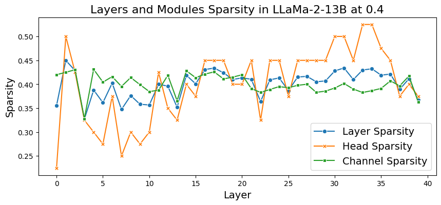
Figure 4: Channels, heads, and layers sparsities.

5.3 Analysis of the Post-Pruning Modules

As global and heterogeneous pruning is performed through our optimization, it is interesting to investigate the pruned modules in each layer. We show the channel, heads, and layers sparsity (i.e., the pruned portion of the corresponding granularity) on LLaMA-2-13B with channels and heads pruning at 40% in Fig. 4. Those results on LLaMA-2-7B are shown in Fig. A1 of Appendix F.

Figures 4 and A1 demonstrate that the pruned LLM exhibits low sparsity in the first and last layers, which is consistent with the previous studies that these layers have a profound impact on the performance of LLMs [36]. Moreover, it can be observed that the heads (of MHA) granularity exhibits lower sparsity in the shallow layers (especially in the first layer), while such observation does not hold for the channels (of MLP) granularity. In other words, the pruned sparsity of the channel granularity is more evenly distributed whereas the deeper layers have a slightly less sparsity. This might imply that the shallow layers focus more on attention, while the deeper layer imposes slightly more responsibility for lifting the feature dimensions through MLP.

6 Discussion and Conclusion

Limitations and Future Works. Firstly, as an optimization-based pruning, though our method exhibits improved performance over the (heuristic) metric-based methods, and a similar memory complexity (approximately 35GB, as only LLM forward is required), it simultaneously requires more training time for optimization (e.g., 2.7 hours for LLaMA-2-13B).

Secondly, there exist advanced policy gradient algorithms with potentially lower variance from the reinforcement learning community [43]. As 1) the primary focus of this paper is on the back-propagation-free formulation of the LLM pruning problem, and 2) our formulation ensures dense rewards at each step, we thus use a basic policy gradient algorithm similar to REINFORCE [53] with simple variance reduction using a moving average baseline. We leave exploiting more powerful policy gradient algorithms as our future work.

Lastly, the performance of the proposed method on specific domains/tasks can rely heavily on the availability of domain-specific datasets. Though the cross-dataset evaluation is verified w.r.t. perplexity, using only the C4 dataset for pruning might introduce a negative influence on other cross-dataset zero-shot tasks such as WinoGrande [42] and Hellaswag [59] shown in the Appendix G.

Conclusion. We propose an efficient optimization-based structural pruning method for LLMs, which 1) does not need back-propagation through the LLM per se, 2) enables global and heterogeneous pruning throughout the LLM, and 3) supports pruning granularities of channels, heads, and layers. Our method can take a metric-based pruning as initialization to achieve an further improved performance. We implement our method by learning an underlying Bernoulli distribution of binary pruning mask. As we decouple the Bernoulli parameter and the sampled masks from the LLM loss, the Bernoulli distribution can thus be optimized by a policy gradient estimator without back-propagation through the LLM. Our method operates for 2.7 hours with approximately 35GB of memory on a single A100 GPU. Extensive experiments on various LLM models and sizes with detailed ablation analysis validate the promising performance of the proposed method.

Appendix A Projection Operator for Sparsity Constraint and the Overall Algorithm

Details of the Projection Operator. In our proposed probabilistic framework, the sparsity constraint manifests itself in a feasible domain on the probability space defined in Problem (3). We denote the feasible domain as $\mathcal{C}=\left\{\mathbf{1}^{\top}\mathbf{s}\leq K\right\}\bigcap\left\{\mathbf{s}\in[0,1]^{n}\right\}$. The theorem [51] below shows that the projection of a vector onto $C$ can be calculated efficiently.

Theorem 1.

For each vector $\mathbf{z}$ , its projection $\textbf{proj}_{\mathcal{C}}(\mathbf{z})$ in the set $C$ can be calculated as follows:

$$\textbf{proj}_{\mathcal{C}}(\mathbf{z})=\text{min}(1,\text{max}(0,\mathbf{z}-v_{2}^{*}\mathbf{1}))$$ (9)

where $v_{2}^{*}=max(0,v_{1}^{*})$ with $v_{1}^{*}$ being the solution of the following equation

$$\mathbf{1}^{T}\left[\text{min}(1,\text{max}(0,\mathbf{z}-v_{1}^{*}\mathbf{1}))\right]-K=0$$ (10)

Equation (9) can be solved by the bisection method efficiently.

The theorem above as well as its proof is standard and it is a special case of the problem stated in [51]. This component, though not the highlight of our work, is included for the reader’s convenience and completeness.

Algorithm. The pseudo-code of our overall algorithm is detailed below.

Algorithm 1 Pseudo-code of PG pruning

0:  target remaining ratio $r>0$, a dense pretrained network $\mathbf{w}$, the step size $\eta>0$, mini-batch size $B>0$, moving average window size $T$, and calibration dataset $\mathcal{D}$

0:  Init probability $\mathbf{s}$ from any pruning metric $\mathbf{x}$, ans set moving average $\delta=0$

1:  while until convergence do

2:     Sample a mini-batch from the entire calibration dataset: $\mathcal{D}_{B}=\{(\mathbf{x}_{i},\mathbf{y}_{i})\}^{B}_{i=1}\sim\mathcal{D}$

3:     Sample $\mathbf{m}^{(i)}$ from $p(\mathbf{m}|s)$, $i=1,2,\dots,N_{s}$

4:     Update the moving average baseline $\delta$ via Eq. (8)

5:     Uptate $\mathbf{s}$ via Eqs. (7), (9), and (10).

6:  end while

Appendix B A Reinforcement Learning Perspective

Our formulation can also be interpreted from the dense-reward model-free reinforcement learning perspective. Particularly, the heavy LLM can be viewed as the agnostic and fixed environment.

In terms of the Markov Decision Process (MDP) (action $a$, states $s$, state transition probability $p$, reward $r$, discount factor $\gamma$), the environment takes the action $a$ sampled from the current Bernoulli policy $\pi$ to insert the binary masks for pruning, produces the states $s$ as the masked/pruned network deterministically (i.e., the state transition probability $p$ is constantly 1), and generate the stepwise dense reward $r$ as the performance (e.g., the cross-entropy loss) of the pruned LLM. Since our problem exhibits dense rewards, therefore the discount factor $\gamma$ is 1.

As a result, our policy to take actions, i.e., the Bernoulli distribution to sample the binary masks, can be learned efficiently exploiting the policy gradient estimator (similar to REINFORCE), without back-propagating through the agnostic and fixed environment of the heavy LLM.

Appendix C More Results of Different Initializations

Progressive Pruning with Random (Random-Progressive) Initialization. Our progressive pruning with random initialization is inspired by the facts that 1) the continous Bernoulli probability learned by our method indicates the importance of the corresponding module, therefore the continous probability scores from a low pruning rate (e.g., 10%) encodes fatal information and can be naturally used as the initialization for a higher pruning rate (e.g., 15%); and 2) the LLMs is likely to exhibit large redundancy when the pruning rate is extremely low (e.g., 5%), thus random initialization will not significantly degrade the pruning performance (compared to a carefully chosen metric-based pruning initialization) given an extremely low pruning rate such as 5%. Therefore, to validate our method without a prior metric-based initialization, we propose a progressive pruning strategy, by starting from 5% pruning rate with random initialization and progressively pruning rate to 50% by a step size of 5%. We train this strategy with each pruning rate for 1/3 epoch to maintain the efficiency.

In addition to Table 3 of Sect. 5.1, Table A1 shows the layer pruning results with different initializations on LLaMA-2-7B.

Table A1: Layer pruning results with different initializations using LLaMA-2-7B. Bold and Underscored denote the first and second best results, respectively.

Method	PruneRate	Perplexity	PruneRate	Perplexity	PruneRate	Perplexity
Layerwise-PPL	30$\%$	24.83	40$\%$	41.45	50$\%$	126.08
Ours (Random Init)	30$\%$	26.65	40$\%$	42.76	50$\%$	125.20
Ours (Random-Prog. Init)		30.05		38.28		111.87
Ours (Layerwise-PPL Init)	30$\%$	23.20	40$\%$	38.26	50$\%$	104.37

Appendix D Projection Strategy for Initialization: From Metric to Probability

As the initialization of our Bernoulli policy should be probabilistic values between 0 and 1, but the metrics calculated by the metric-based methods [46, 2, 36] may not hold this range, we thus need to project those metric values to [0, 1] as our initialization. We introduce two projection strategies from metric values $\mathbf{m}$ to probabilities $\mathbf{s}$. The first is called Sigmoid-Norm strategy, which is applied in our main experiments:

$$\mathbf{s}=\text{sigmoid}(\text{Norm}(\mathbf{x}))$$ (11)

where $\text{Norm}(\cdot)$ is used to linearly normalize the input to a Gaussian distribution with 0 mean and unit variance, then $sigmoid(\cdot)$ is used to transform the input to $[0,1]$.

An alternative second strategy is named Score-Const. It straightforwardly sets the mask 1 from metric-based methods as a constant $c$, and mask 0 as $1-c$:

$$s_{i}=\left\{\begin{aligned} &c,&\mathrm{if}\,\,m_{i}=1,\\ &1-c,&\mathrm{if}\,\,m_{i}=0,\end{aligned}\right.$$ (12)

The constant $c$ is set to 0.8 in the following experiments, indicating that the initialized Bernoulli probability of the remaining modules is 0.8 and those to be pruned is 0.2.

The results of different projection strategies on LLaMA-2-7B/13B are detailed in Table A2, which shows that the Sigmoid-Norm projection outperforms its Score-Const counterpart for most cases. It may be because the order-preserving projection strategy of Sigmoid-Norm preserves more information about relative importance among modules, and therefore benefits the optimization.

Table A2: Results with different projection strategies for pruning heads, channels, and layers on LLaMA-2-7B/13B. Initialization metrics are from Wanda-sp for heads/channels and Layerwise-PPL for layers.

(a) Channels and heads pruning.

Method	Sparsity	7B	13B
Sigmoid-Norm	30$\%$	28.18	21.99
Score-Const		32.25	25.38
Sigmoid-Norm	35$\%$	32.52	26.27
Score-Const		40.61	40.51
Sigmoid-Norm	40$\%$	39.81	31.52
Score-Const		44.46	52.10
Sigmoid-Norm	45$\%$	52.07	40.99
Score-Const		65.31	61.04
Sigmoid-Norm	50$\%$	65.21	52.23
Score-Const		77.07	88.72

(b) Layer pruning.

Method	Sparsity	7B	13B
Sigmoid-Norm	30$\%$	23.20	21.93
Score-Const		25.32	19.31
Sigmoid-Norm	35$\%$	33.27	26.46
Score-Const		31.37	23.40
Sigmoid-Norm	40$\%$	38.26	30.99
Score-Const		42.30	29.25
Sigmoid-Norm	45$\%$	69.23	39.26
Score-Const		63.91	39.50
Sigmoid-Norm	50$\%$	104.37	69.92
Score-Const		135.51	54.37

Appendix E Additional Results of Our Pruning Method

In compensating for the results from Tables 1 and 2, we also present the results of additional pruning rates of 35% and 45% for channels and heads pruning, as well as layer pruning, in Table A3 and Table A4. These results demonstrate the consistent improvement of our proposed method across various pruning rates.

Table A3: Results on channels and heads pruning under prune rates of 35% and 45%.

Method	PruneRate	LLaMA		LLaMA-2		Vicuna
		7B	13B	7B	13B	7B	13B
LLM-Pruner	35$\%$	49.71	28.82	50.00	30.80	63.58	37.16
SliceGPT		-	-	54.57	39.83	67.79	86.37
Wanda-sp		48.39	72.55	60.87	125.61	70.19	190.62
Ours		31.81	24.57	32.52	26.27	42.32	32.18
LLM-Pruner	45$\%$	96.95	50.39	130.97	53.33	125.46	64.58
SliceGPT		-	-	116.07	67.68	122.27	180.96
Wanda-sp		446.556	216.13	104.65	153.08	98.02	262.22
Ours		65.39	34.63	52.07	40.99	56.90	51.74

Table A4: Results on layers pruning under prune rates of 35% and 45%.

Method	PruneRate	LLaMA		LLaMA-2		Vicuna
		7B	13B	7B	13B	7B	13B
Layerwise-PPL	35$\%$	54.66	33.34	34.56	24.19	53.23	38.51
Ours		36.15	31.32	33.27	26.46	37.55	28.36
Layerwise-PPL	45$\%$	69.27	110.40	70.73	44.83	152.87	85.30
Ours		56.14	49.66	69.23	39.26	78.56	50.79

Appendix F Analysis of the Post-Pruning Modules on LLaMA-2-7B

Besides the LLaMA-2-13B results in Fig. 4 of Sect. 5.3, the channels, heads, and layers sparsities on LLaMA-2-7B with channels and heads pruning are shown in Fig. A1, which illustrates a similar observation as Fig. 4.

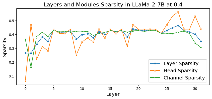
Figure A1: Channels, heads, and layers sparsities on LLaMA-2-7B.

Appendix G Zero-shot Performance on Other NLP tasks

We follow SliceGPT [3] to assess our pruned LLM on five zero-shot tasks: PIQA [4], WinoGrande [42], HellaSwag [59], ARC-e and ARC-c [11] by EleutherAI LM Harness [18]. The task-wise performance and the averaging zero-shot accuracies using LLaMA-2-7B are presented in Table A5.

Table A5: Accuracies ($\%$) of LLaMA-2-7B for 5 zero-shot tasks with pruning rates from 30$\%$ to 50$\%$

Method	PruneRate	PIQA	HellaSwag	WinoGrande	ARC-e	ARC-c	Average
LLM-Pruner	30$\%$	71.81	43.64	54.06	63.42	30.30	52.64
SliceGPT		72.31	60.11	63.22	53.10	32.00	56.15
Ours		75.41	50.34	61.60	66.03	35.58	57.79
LLM-Pruner	40$\%$	67.52	35.76	51.70	48.31	24.65	45.59
SliceGPT		65.40	48.91	60.38	42.13	26.88	48.74
Ours		71.11	42.44	55.72	56.94	28.50	50.94
LLM-Pruner	50$\%$	59.52	29.74	50.11	36.48	21.84	39.54
SliceGPT		59.47	37.96	56.27	33.63	22.78	42.02
Ours		61.80	30.94	52.40	40.11	20.47	41.14

Appendix H Training Time and Memory Statistics

Our training times for channel and head pruning on LLaMA-2-7B and LLaMA-2-13B are 1.76 and 2.72 hours, respectively. Although our method is slower than metric-based methods such as Wanda-sp [2], the trade-off is justified by the substantial performance enhancements delivered by our optimization-based approach.

The GPU memory requirements for channel and head pruning on LLaMA-2-7B and LLaMA-2-13B for our methods, as well as the representative metric-based method, i.e., Wanda-sp, are illustrated in Table A6. We do not compare it to LLM-Pruner and SliceGPT because 1) the LLM-Pruner requires much more memory for back-propagation (therefore the authors also used the CPU memory), 2) the original implementation of SliceGPT also used both CPU and GPU memory for computations. Table A6 shows that our method exhibits a similar GPU memory requirement to the efficient Wanda-sp, as we only need the forward pass of the LLM. The slight additional memory required by our method comes from the need to store the Bernoulli parameters $\mathbf{s}$ and the sampled masks $\mathbf{m}$.

Table A6: Memory requirements (GB) for channel and head pruning on LLaMA-2-7B/13B.

Method	7B		13B
	Min	Max	Min	Max
Wanda-sp	17.5	20.3	29.5	36.9
Ours	18.2	19.5	34.1	35.8

Appendix I Random Error Statistic

The standard deviation statistics of our method are shown in Table A7. Theoretically, the variance is induced by stochastic sampling from Bernoulli distribution in the policy gradient optimization if the initialization is fixed. Therefore, we fixed the initialization as Wanda-sp to calculate the standard deviation of the proposed method. Experiments of head and channel pruning, along with layer pruning, are executed using LLaMA-2-7B for 10 run trials. Table A7 shows that our method possesses a reasonable standard deviation.

Table A7: Mean and standard deviation of our method for LLaMA-2-7B.

Granularity	PruneRate
	30%	40%	50%
Head and Channel	28.18 $\pm$ 1.83	39.81 $\pm$ 1.41	65.21$\pm$ 2.52
Layer	23.20 $\pm$ 0.67	38.26 $\pm$ 2.68	104.37 $\pm$ 1.05

Appendix J Broader Impacts

We have introduced an efficient pruning method tailored for LLMs, which aims to accelerate the inference time of LLMs. Given the frequent calls to online-deployed LLMs such as ChatGPT, our approach offers an energy-efficient positive impact, which also helps to enhance user experience. Additionally, it shares both the positive and negative broader impacts inherent to LLM technology.

References

- [1] Josh Achiam, Steven Adler, Sandhini Agarwal, Lama Ahmad, Ilge Akkaya, Florencia Leoni Aleman, Diogo Almeida, Janko Altenschmidt, Sam Altman, Shyamal Anadkat, et al. Gpt-4 technical report. arXiv preprint arXiv:2303.08774, 2023.
- [2] Yongqi An, Xu Zhao, Tao Yu, Ming Tang, and Jinqiao Wang. Fluctuation-based adaptive structured pruning for large language models. arXiv preprint arXiv:2312.11983, 2023.
- [3] Saleh Ashkboos, Maximilian L Croci, Marcelo Gennari do Nascimento, Torsten Hoefler, and James Hensman. Slicegpt: Compress large language models by deleting rows and columns. arXiv preprint arXiv:2401.15024, 2024.
- [4] Yonatan Bisk, Rowan Zellers, Jianfeng Gao, Yejin Choi, et al. Piqa: Reasoning about physical commonsense in natural language. In Proceedings of the AAAI conference on artificial intelligence, volume 34, pages 7432–7439, 2020.
- [5] Davis Blalock, Jose Javier Gonzalez Ortiz, Jonathan Frankle, and John Guttag. What is the state of neural network pruning? In MLSys, pages 129–146, 2020.
- [6] Vladimír Boža. Fast and optimal weight update for pruned large language models. arXiv preprint arXiv:2401.02938, 2024.
- [7] Tom Brown, Benjamin Mann, Nick Ryder, Melanie Subbiah, Jared D Kaplan, Prafulla Dhariwal, Arvind Neelakantan, Pranav Shyam, Girish Sastry, Amanda Askell, et al. Language models are few-shot learners. In NeurIPS, pages 1877–1901, 2020.
- [8] Tianyi Chen, Tianyu Ding, Badal Yadav, Ilya Zharkov, and Luming Liang. Lorashear: Efficient large language model structured pruning and knowledge recovery. arXiv preprint arXiv:2310.18356, 2023.
- [9] Xiaodong Chen, Yuxuan Hu, and Jing Zhang. Compressing large language models by streamlining the unimportant layer. arXiv preprint arXiv:2403.19135, 2024.
- [10] Wei-Lin Chiang, Zhuohan Li, Zi Lin, Ying Sheng, Zhanghao Wu, Hao Zhang, Lianmin Zheng, Siyuan Zhuang, Yonghao Zhuang, Joseph E. Gonzalez, Ion Stoica, and Eric P. Xing. Vicuna: An open-source chatbot impressing gpt-4 with 90%* chatgpt quality, 2023.
- [11] Peter Clark, Isaac Cowhey, Oren Etzioni, Tushar Khot, Ashish Sabharwal, Carissa Schoenick, and Oyvind Tafjord. Think you have solved question answering? try arc, the ai2 reasoning challenge. arXiv preprint arXiv:1803.05457, 2018.
- [12] Rocktim Jyoti Das, Liqun Ma, and Zhiqiang Shen. Beyond size: How gradients shape pruning decisions in large language models. arXiv preprint arXiv:2311.04902, 2023.
- [13] Lucio Dery, Steven Kolawole, Jean-Francois Kagey, Virginia Smith, Graham Neubig, and Ameet Talwalkar. Everybody prune now: Structured pruning of llms with only forward passes. arXiv preprint arXiv:2402.05406, 2024.
- [14] Utku Evci, Trevor Gale, Jacob Menick, Pablo Samuel Castro, and Erich Elsen. Rigging the lottery: Making all tickets winners. In ICML, pages 2943–2952, 2020.
- [15] Jonathan Frankle and Michael Carbin. The lottery ticket hypothesis: Finding sparse, trainable neural networks. arXiv preprint arXiv:1803.03635, 2018.
- [16] Elias Frantar and Dan Alistarh. Sparsegpt: Massive language models can be accurately pruned in one-shot. In ICML, pages 10323–10337, 2023.
- [17] Trevor Gale, Erich Elsen, and Sara Hooker. The state of sparsity in deep neural networks. arXiv preprint arXiv:1902.09574, 2019.
- [18] Leo Gao, Jonathan Tow, Baber Abbasi, Stella Biderman, Sid Black, Anthony DiPofi, Charles Foster, Laurence Golding, Jeffrey Hsu, Alain Le Noac’h, Haonan Li, Kyle McDonell, Niklas Muennighoff, Chris Ociepa, Jason Phang, Laria Reynolds, Hailey Schoelkopf, Aviya Skowron, Lintang Sutawika, Eric Tang, Anish Thite, Ben Wang, Kevin Wang, and Andy Zou. A framework for few-shot language model evaluation, 12 2023.
- [19] Mitchell Gordon, Kevin Duh, and Nicholas Andrews. Compressing bert: Studying the effects of weight pruning on transfer learning. In ACL Workshop, pages 143–155, 2020.
- [20] Song Guo, Jiahang Xu, Li Lyna Zhang, and Mao Yang. Compresso: Structured pruning with collaborative prompting learns compact large language models. arXiv preprint arXiv:2310.05015, 2023.
- [21] Song Han, Huizi Mao, and William J Dally. Deep compression: Compressing deep neural networks with pruning, trained quantization and huffman coding. arXiv preprint arXiv:1510.00149, 2015.
- [22] Babak Hassibi and David Stork. Second order derivatives for network pruning: Optimal brain surgeon. In NIPS, 1992.
- [23] Yang He, Guoliang Kang, Xuanyi Dong, Yanwei Fu, and Yi Yang. Soft filter pruning for accelerating deep convolutional neural networks. arXiv preprint arXiv:1808.06866, 2018.
- [24] Edward J Hu, Yelong Shen, Phillip Wallis, Zeyuan Allen-Zhu, Yuanzhi Li, Shean Wang, Lu Wang, and Weizhu Chen. Lora: Low-rank adaptation of large language models. arXiv preprint arXiv:2106.09685, 2021.
- [25] Zehao Huang and Naiyan Wang. Data-driven sparse structure selection for deep neural networks. In ECCV, pages 304–320, 2018.
- [26] Ajay Jaiswal, Shiwei Liu, Tianlong Chen, and Zhangyang Wang. The emergence of essential sparsity in large pre-trained models: The weights that matter. arXiv preprint arXiv:2306.03805, 2023.
- [27] Bo-Kyeong Kim, Geonmin Kim, Tae-Ho Kim, Thibault Castells, Shinkook Choi, Junho Shin, and Hyoung-Kyu Song. Shortened llama: A simple depth pruning for large language models. arXiv preprint arXiv:2402.02834, 2024.
- [28] Jongwoo Ko, Seungjoon Park, Yujin Kim, Sumyeong Ahn, Du-Seong Chang, Euijai Ahn, and Se-Young Yun. Nash: A simple unified framework of structured pruning for accelerating encoder-decoder language models. arXiv preprint arXiv:2310.10054, 2023.
- [29] Eldar Kurtic, Daniel Campos, Tuan Nguyen, Elias Frantar, Mark Kurtz, Benjamin Fineran, Michael Goin, and Dan Alistarh. The optimal bert surgeon: Scalable and accurate second-order pruning for large language models. arXiv preprint arXiv:2203.07259, 2022.
- [30] Shengrui Li, Xueting Han, and Jing Bai. Nuteprune: Efficient progressive pruning with numerous teachers for large language models. arXiv preprint arXiv:2402.09773, 2024.
- [31] Yun Li, Lin Niu, Xipeng Zhang, Kai Liu, Jianchen Zhu, and Zhanhui Kang. E-sparse: Boosting the large language model inference through entropy-based N: M sparsity. arXiv preprint arXiv:2310.15929, 2023.
- [32] Liyang Liu, Shilong Zhang, Zhanghui Kuang, Aojun Zhou, Jing-Hao Xue, Xinjiang Wang, Yimin Chen, Wenming Yang, Qingmin Liao, and Wayne Zhang. Group fisher pruning for practical network compression. In ICML, pages 7021–7032, 2021.
- [33] Yanli Liu, Kaiqing Zhang, Tamer Basar, and Wotao Yin. An improved analysis of (variance-reduced) policy gradient and natural policy gradient methods. Advances in Neural Information Processing Systems, 33:7624–7636, 2020.
- [34] Zhuang Liu, Mingjie Sun, Tinghui Zhou, Gao Huang, and Trevor Darrell. Rethinking the value of network pruning. arXiv preprint arXiv:1810.05270, 2018.
- [35] Christos Louizos, Max Welling, and Diederik P Kingma. Learning sparse neural networks through regularization. arXiv preprint arXiv:1712.01312, 2017.
- [36] Xinyin Ma, Gongfan Fang, and Xinchao Wang. Llm-pruner: On the structural pruning of large language models. arXiv preprint arXiv:2305.11627, 2023.
- [37] Chris J Maddison, Andriy Mnih, and Yee Whye Teh. The concrete distribution: A continuous relaxation of discrete random variables. arXiv preprint arXiv:1611.00712, 2016.
- [38] Xin Men, Mingyu Xu, Qingyu Zhang, Bingning Wang, Hongyu Lin, Yaojie Lu, Xianpei Han, and Weipeng Chen. Shortgpt: Layers in large language models are more redundant than you expect. arXiv preprint arXiv:2403.03853, 2024.
- [39] Stephen Merity, Caiming Xiong, James Bradbury, and Richard Socher. Pointer sentinel mixture models. arXiv preprint arXiv:1609.07843, 2016.
- [40] Pavlo Molchanov, Arun Mallya, Stephen Tyree, Iuri Frosio, and Jan Kautz. Importance estimation for neural network pruning. In CVPR, pages 11264–11272, 2019.
- [41] Colin Raffel, Noam Shazeer, Adam Roberts, Katherine Lee, Sharan Narang, Michael Matena, Yanqi Zhou, Wei Li, and Peter J Liu. Exploring the limits of transfer learning with a unified text-to-text transformer. JMLR, 21(140):1–67, 2020.
- [42] Keisuke Sakaguchi, Ronan Le Bras, Chandra Bhagavatula, and Yejin Choi. Winogrande: An adversarial winograd schema challenge at scale. Communications of the ACM, 64(9):99–106, 2021.
- [43] John Schulman, Filip Wolski, Prafulla Dhariwal, Alec Radford, and Oleg Klimov. Proximal policy optimization algorithms. arXiv preprint arXiv:1707.06347, 2017.
- [44] Hang Shao, Bei Liu, and Yanmin Qian. One-shot sensitivity-aware mixed sparsity pruning for large language models. arXiv preprint arXiv:2310.09499, 2023.
- [45] Dachuan Shi, Chaofan Tao, Ying Jin, Zhendong Yang, Chun Yuan, and Jiaqi Wang. Upop: Unified and progressive pruning for compressing vision-language transformers. In ICML, pages 31292–31311, 2023.
- [46] Mingjie Sun, Zhuang Liu, Anna Bair, and J Zico Kolter. A simple and effective pruning approach for large language models. arXiv preprint arXiv:2306.11695, 2023.
- [47] Hugo Touvron, Thibaut Lavril, Gautier Izacard, Xavier Martinet, Marie-Anne Lachaux, Timothée Lacroix, Baptiste Rozière, Naman Goyal, Eric Hambro, Faisal Azhar, et al. Llama: Open and efficient foundation language models. arXiv preprint arXiv:2302.13971, 2023.
- [48] Hugo Touvron, Louis Martin, Kevin Stone, Peter Albert, Amjad Almahairi, Yasmine Babaei, Nikolay Bashlykov, Soumya Batra, Prajjwal Bhargava, Shruti Bhosale, et al. Llama 2: Open foundation and fine-tuned chat models. arXiv preprint arXiv:2307.09288, 2023.
- [49] Tycho FA van der Ouderaa, Markus Nagel, Mart van Baalen, Yuki M Asano, and Tijmen Blankevoort. The llm surgeon. arXiv preprint arXiv:2312.17244, 2023.
- [50] Huan Wang, Can Qin, Yulun Zhang, and Yun Fu. Neural pruning via growing regularization. In ICLR, 2021.
- [51] Weiran Wang and Miguel A Carreira-Perpinán. Projection onto the probability simplex: An efficient algorithm with a simple proof, and an application. arXiv preprint arXiv:1309.1541, 2013.
- [52] Boyi Wei, Kaixuan Huang, Yangsibo Huang, Tinghao Xie, Xiangyu Qi, Mengzhou Xia, Prateek Mittal, Mengdi Wang, and Peter Henderson. Assessing the brittleness of safety alignment via pruning and low-rank modifications. arXiv preprint arXiv:2402.05162, 2024.
- [53] Ronald J Williams. Simple statistical gradient-following algorithms for connectionist reinforcement learning. Machine learning, 8:229–256, 1992.
- [54] Haojun Xia, Zhen Zheng, Yuchao Li, Donglin Zhuang, Zhongzhu Zhou, Xiafei Qiu, Yong Li, Wei Lin, and Shuaiwen Leon Song. Flash-llm: Enabling cost-effective and highly-efficient large generative model inference with unstructured sparsity. arXiv preprint arXiv:2309.10285, 2023.
- [55] Mengzhou Xia, Tianyu Gao, Zhiyuan Zeng, and Danqi Chen. Sheared llama: Accelerating language model pre-training via structured pruning. arXiv preprint arXiv:2310.06694, 2023.
- [56] Peng Xu, Wenqi Shao, Mengzhao Chen, Shitao Tang, Kaipeng Zhang, Peng Gao, Fengwei An, Yu Qiao, and Ping Luo. Besa: Pruning large language models with blockwise parameter-efficient sparsity allocation. arXiv preprint arXiv:2402.16880, 2024.
- [57] Yifei Yang, Zouying Cao, and Hai Zhao. Laco: Large language model pruning via layer collapse. arXiv preprint arXiv:2402.11187, 2024.
- [58] Lu Yin, You Wu, Zhenyu Zhang, Cheng-Yu Hsieh, Yaqing Wang, Yiling Jia, Mykola Pechenizkiy, Yi Liang, Zhangyang Wang, and Shiwei Liu. Outlier weighed layerwise sparsity (owl): A missing secret sauce for pruning llms to high sparsity. arXiv preprint arXiv:2310.05175, 2023.
- [59] Rowan Zellers, Ari Holtzman, Yonatan Bisk, Ali Farhadi, and Yejin Choi. Hellaswag: Can a machine really finish your sentence? arXiv preprint arXiv:1905.07830, 2019.
- [60] Hongchuan Zeng, Hongshen Xu, Lu Chen, and Kai Yu. Multilingual brain surgeon: Large language models can be compressed leaving no language behind. arXiv preprint arXiv:2404.04748, 2024.
- [61] Mingyang Zhang, Hao Chen, Chunhua Shen, Zhen Yang, Linlin Ou, Xinyi Yu, and Bohan Zhuang. Loraprune: Pruning meets low-rank parameter-efficient fine-tuning. arXiv preprint arXiv:2305.18403, 2023.
- [62] Yingtao Zhang, Haoli Bai, Haokun Lin, Jialin Zhao, Lu Hou, and Carlo Vittorio Cannistraci. Plug-and-play: An efficient post-training pruning method for large language models. In ICLR, 2024.
- [63] Yuxin Zhang, Lirui Zhao, Mingbao Lin, Yunyun Sun, Yiwu Yao, Xingjia Han, Jared Tanner, Shiwei Liu, and Rongrong Ji. Dynamic sparse no training: Training-free fine-tuning for sparse llms. arXiv preprint arXiv:2310.08915, 2023.
- [64] Bowen Zhao, Hannaneh Hajishirzi, and Qingqing Cao. Apt: Adaptive pruning and tuning pretrained language models for efficient training and inference. arXiv preprint arXiv:2401.12200, 2024.
- [65] Chenglong Zhao, Bingbing Ni, Jian Zhang, Qiwei Zhao, Wenjun Zhang, and Qi Tian. Variational convolutional neural network pruning. In CVPR, pages 2780–2789, 2019.
- [66] Michael Zhu and Suyog Gupta. To prune, or not to prune: exploring the efficacy of pruning for model compression. arXiv preprint arXiv:1710.01878, 2017.