An Adaptive Method for Non-Stationary Stochastic Multi-armed Bandits with Rewards Generated by a Linear Dynamical System

Abstract

Online decision-making can be formulated as the popular stochastic multi-armed bandit problem where a learner makes decisions (or takes actions) to maximize cumulative rewards collected from an unknown environment. A specific variant of the bandit problem is the non-stationary stochastic multi-armed bandit problem, where the reward distributions—which are unknown to the learner—change over time. This paper proposes to model non-stationary stochastic multi-armed bandits as an unknown stochastic linear dynamical system as many applications, such as bandits for dynamic pricing problems or hyperparameter selection for machine learning models, can benefit from this perspective. Following this approach, we can build a matrix representation of the system’s steady-state Kalman filter that takes a set of previously collected observations from a time interval of length $s$ to predict the next reward that will be returned for each action. This paper proposes a solution in which the parameter $s$ is determined via an adaptive algorithm by analyzing the model uncertainty of the matrix representation. This algorithm helps the learner adaptively adjust its model size and its length of exploration based on the uncertainty of its environmental model. The effectiveness of the proposed scheme is demonstrated through extensive numerical studies, revealing that the proposed scheme is capable of increasing the rate of collected cumulative rewards.

I Introduction

The stochastic multi-armed bandit problem focuses on modeling online learning processes to understand decision-making under uncertainty with the aim of providing a simplified framework to a situation encountered frequently. The problem considers a learner interacting with an environment, where the learner chooses an action for which the environment in return gives a reward that is sampled from a probability distribution. Performance is usually measured in terms of cumulative regret, i.e. the cumulative difference between the highest reward that could be given for a round and the reward given for the chosen action. Since it is assumed that the learner lacks prior knowledge about the environment [1], the learner needs to balance between exploring each action to extract information and committing to an action to maximize cumulative reward. A popular adaptive exploration method that has been introduced where the distributions are assumed to be stationary is the Upper Confidence Bound (UCB) method [2].

In the case of non-stationary stochastic multi-armed bandits, it is assumed that the distributions of the rewards can change over time [1]. Therefore, learners need to understand how its previous information of the environment may misrepresent the current reward distributions. Most of the previous methods have focused on piece-wise stationary cases, where the distribution shifts abruptly [3]. In this context, presented algorithms are commonly approached as a forgetting versus memorizing trade-off, where either the estimates of the reward distributions are forgotten when a distributional shift is detected [4, 5, 6, 7] or the estimates of the reward distributions use measurements that are within a sliding window [3]. The piece-wise stationary stochastic multi-armed bandits have also been considered for the linear bandits; the linear bandit is when the reward is the inner product of an unknown vector and an action vector chosen by the learner [8]. Prior work has considered the cases where the unknown parameter vector changes abruptly [9], and where the rewards are dependent on the previously chosen action vectors [10]. Some non-stationary methods focused on the impact of distributional change in the form of variational budget, which is a known constant that bounds the cumulative changes in the distributions [11, 12]. In contrast to piece-wise stationary cases, the distribution may change slowly, which are referred as slowly-varying case [13]. For the slowly-varying case, the restless bandit is introduced in [14], where the rewards from each arm evolves as a Markov process; this can be further specified to be a reward process that is modeled as Brownian motion [15]. The approach has been extended to the scenarios where the rewards are generated by a partially observable stochastic linear dynamical system [16].

For this work, we consider the slowly-varying case as it has many applications. For example, applications that have been introduced for slowly varying non-stationary stochastic multi-armed bandits include dynamic pricing problem [17, 18], controller selection for time-varying stochastic linear dynamical system [19], opportunistic spectrum access in wireless networks [20], and hyperparameter optimization [21] or algorithm selection [22] for machine learning models. We argue that each of the applications above can be modeled as a dynamical system, which is a specific variation of the slowly-varying case. In addition, previous works have made a similar assumption. For example, previous results that have assumed an underlying dynamical system for the bandit environment are [18] for dynamic pricing, [23] for hyperparameter optimization, and [19] for controller selection.

Building upon the authors’ previous work [16], this paper develops an adaptive algorithm that maximizes cumulative rewards sampled from an unknown stochastic linear dynamical system. We develop a method that adaptively chooses the model size, which denotes the number of previous observations to be taken into account, and the length of exploration based on the uncertainty of the model that the learner has learned for the environment. Such features allow the learner explore the environment adaptively. This addresses the weakness of PIES, the algorithm proposed in [16], where the window size and exploration length of the environment are preset, which can lead to a situation where the exploration length is longer than the horizon length. Therefore, this paper provides a perspective on how learners should integrate model selection with its decisions on whether to explore the environment versus commit to an action.

This paper is organized as follows. Section II states the problem. In Section III, a methodology to model and predict rewards is presented and Section IV discusses how model size and its errors can impact performance. Section V uses the learned model to develop a strategy to maximize cumulative reward over a horizon. Section VI performs regret analysis and provides a theoretical upper bound for the regret. Finally, Section VII has numerical results and Section VIII concludes the paper and provides future directions.

II Problem Statement

Suppose that for $k$ given actions $c_{a}\in\mathscr{A}\triangleq\{c_{a}\in\mathbb{R}^{d}\mid a=1,2,\dots,k\}$, the reward $X_{t}$ is sampled from the following linear Gaussian dynamical system

$$\begin{cases}z_{t+1}&=\Gamma z_{t}+\xi_{t},~{}z_{0}\sim\mathscr{N}(0,\Sigma_{0})\\ \theta_{t}&=C_{\theta}z_{t}+\phi_{t}\\ X_{t}&=\langle c_{a},z_{t}\rangle+\eta_{t}\end{cases},$$ (1)

where $z_{t}\in\mathbb{R}^{d}$ is the state of the system and $\Gamma\in\mathbb{R}^{d\times d}$ is the system state matrix. For each round $t=1,2,\dots,n$ and $n>d$, the learner observes the reward $X_{t}\in\mathbb{R}$ based on the chosen action and the context $\theta_{t}\in\mathbb{R}^{m}$. The context $\theta_{t}$ is a value that the learner always observes and its observation matrix $C_{\theta}\in\mathbb{R}^{m\times d}$ is constant. The noises $\xi_{t}\in\mathbb{R}^{d}$, $\phi_{t}\in\mathbb{R}^{m}$, and $\eta_{t}\in\mathbb{R}$ are i.i.d. normally distributed, i.e., $\xi_{t}\sim\mathscr{N}(\mu,Q)$ with $Q\succeq 0$, $\phi_{t}\sim\mathscr{N}(0,R)$ with $R\succ 0$, and $\eta_{t}\sim\mathscr{N}(0,\sigma_{\eta})$ with $\sigma_{\eta}>0$.

Assumption 1.

The matrices $\Gamma$, $C_{\theta}$, $Q$, $R$, $\Sigma_{0}$, vectors $\mu$, and scalar $\sigma_{\eta}$ are unknown. The dimension $d$ is unknown, but dimension $m$ is known as it is the dimension of the context. Also, the vector $c_{a}$ is unknown. Note that for notation, given that there are $k$ vectors $c_{a}\in\mathscr{A}$, we denote $a\in[k]$ to be which vector $c_{a}$ is chosen (for natural numbers $i\in\mathbb{N}$, $[i]\triangleq\{1,2,\dots,i\}$ [1]).

Assumption 2.

The matrix $\Gamma$ is marginally stable for all $t\geq 0$ (i.e., eigenvalues of $\Gamma$ are within and on the unit circle). Also, the pair $(\Gamma,C_{\theta})$ is observable and the pair $(\Gamma,Q^{1/2})$ is controllable.

The goal of the learner is to maximize cumulative reward over a finite time horizon $n$. To do so, regret analysis is used. The regret is defined as the cumulative, over all rounds, expected difference between the highest reward (denoted as $X_{t}^{\ast}$) and the reward for the chosen action at time $t$, i.e.,

$$R_{n}=\sum_{t=1}^{n}\mathbb{E}\left[X_{t}^{\ast}-X_{t}\right].$$ (2)

III Matrix Representation of the System

If the learner knew parameters of system (1), then they could use the Kalman filter (which is the optimal prediction in the mean-squared sense) expressed in (3) to predict the state $z_{t}$, and consequently the reward $X_{t}$, for each action $a\in[k]$:

$$\left\{\begin{array}[]{ll}\hat{z}_{t+1|t}&=\Gamma\hat{z}_{t|t}+\mu\\ P_{t+1|t}&=\Gamma P_{t|t}\Gamma^{\top}+Q\\ K_{t}&=P_{t|t-1}C_{\theta}^{\top}(C_{\theta}P_{t|t-1}C_{\theta}^{\top}+R)^{-1}\\ \hat{z}_{t|t}&=\hat{z}_{t|t-1}+K_{t}(\theta_{t}-C_{\theta}\hat{z}_{t|t-1})\\ P_{t|t}&=P_{t|t-1}-K_{t}C_{\theta}P_{t|t-1}\\ \hat{X}_{t|t-1}&=\langle c_{a},\hat{z}_{t|t-1}\rangle\end{array}\right.,$$ (3)

where $\hat{z}_{t|t}\triangleq\mathbb{E}\left[z_{t}|\mathscr{F}_{t}\right]$, $P_{t|t}\triangleq\mathbb{E}\left[(z_{t}-\hat{z}_{t|t})(z_{t}-\hat{z}_{t|t})^{\top}|\mathscr{F}_{t}\right]$, and $\mathscr{F}_{t}$ is the sigma algebra generated by previous contexts $\theta_{0},\dots,\theta_{t}$. Since the pair $(\Gamma,C_{\theta})$ is observable (see Assumption 2), the Kalman gain matrix $K_{t}$ converges in few steps [24]. Therefore, the steady-state Kalman filter can be used:

$$\left\{\begin{array}[]{ll}\hat{z}_{t+1}&=\Gamma\hat{z}_{t}+\mu+\Gamma K(\theta_{t}-C_{\theta}\hat{z}_{t})\\ \hat{X}_{t}&=\langle c_{a},\hat{z}_{t}\rangle\end{array}\right.,$$ (4)

where

$$\left\{\begin{array}[]{ll}K&\triangleq PC_{\theta}^{\top}(C_{\theta}PC_{\theta}^{\top}+R_{\phi})^{-1}\\ \hat{z}_{t}&\triangleq\hat{z}_{t|t-1}\\ \hat{X}_{t}&\triangleq\hat{X}_{t|t-1}=\mathbb{E}[X_{t}\mid\mathscr{F}_{t-1}]\end{array}\right..$$ (8)

with $P$ being the solution to the Riccati equation $P=\Gamma P\Gamma^{\top}+Q-\Gamma PC_{\theta}^{\top}(C_{\theta}PC_{\theta}^{\top}+R_{\phi})^{-1}C_{\theta}P\Gamma^{\top}$.

Since system parameters are unknown, taking the inspiration from [24], we develop a method to learn the matrix representation of the Kalman filter. Let $s>0$ be the horizon length of how far we look into the past. We define vectors $G_{a}\left(s\right)$ for each $a\in[k]$ and $\Theta_{t}$ as follows:

$$G_{a}\left(s\right)\triangleq\Bigg{[} c_{a}^{\top}\left(\Gamma-\Gamma KC_{\theta}\right)^{s-1}\Gamma K~{}~{}\cdots~{}~{}c_{a}^{\top}\Gamma K$$

$$\sum_{\tau=1}^{s}\left\langle c_{a},\left(\Gamma-\Gamma KC_{\theta}\right)^{\tau}\mu\right\rangle\Bigg{]}^{\top}\in\mathbb{R}^{(ms+1)\times 1},$$ (9)

$$\Theta_{t}\triangleq\Big{[} \theta_{t-s}^{\top}~{}~{}\cdots~{}~{}\theta_{t-1}^{\top}~{}~{}1\Big{]}^{\top}\in\mathbb{R}^{(ms+1)\times 1}.$$ (10)

Using $G_{a}\left(s\right)$ and $\Theta_{t}$ defined above, the reward $X_{t}$ can be expressed as

$$X_{t} =G_{a}\left(s\right)^{\top}\Theta_{t}+\beta_{a;t}+\varepsilon_{a;t},$$ (11)

where

$$\beta_{a;t} \triangleq\left\langle c_{a},\left(\Gamma-\Gamma KC_{\theta}\right)^{s}\hat{z}_{t-s}\right\rangle,$$ (12)

$$\varepsilon_{a;t} \triangleq\langle c_{a},z_{t}-\hat{z}_{t}\rangle+\eta_{t}\sim\mathscr{N}(0,c_{a}^{\top}Pc_{a}+\sigma_{\eta}).$$ (13)

Remark 1.

According to (11), at round $t$, given the set of contexts from round $t-s$ up to round $t-1$ (i.e., $\{\theta_{t-s},\dots,\theta_{t-1}\}$), one can predict the reward $X_{t}$, where the prediction accuracy is impacted by the terms $\beta_{a;t}$ and $\varepsilon_{a;t}$ given in (12) and (13), respectively.

The following assumptions are imposed for $G_{a}\left(s\right)$ and $\varepsilon_{a;t}$.

Assumption 3.

According to discussions in [25], it is reasonable to assume that there exists a known constant $B_{G}$ such that $\|G_{a}\left(s\right)\|_{2}\leq B_{G}$ for all $a\in[k]$.

Assumption 4.

There exists a known constant $B_{c}>0$ such that $\left\|c_{a}\right\|_{2}\leq B_{c},~{}a\in\{1,\cdots,k\}$.

Assumption 5.

Define the covariance matrix of the system (1) as $Z_{t}\triangleq\mathbb{E}\left[z_{t}z_{t}^{\top}\right]$ which has the iteration $Z_{t+1}=\Gamma Z_{t}\Gamma^{\top}+Q+\mu\mu^{\top}$. We assume that there exists a known constant $B_{R}>0$ such that for any round $t>0$, $\sqrt{\mbox{tr}\left(Z_{t}\right)}\leq B_{R}$. Thus, for $\varepsilon_{a;t}$ as in (13), the variance is bounded such that for any $a\in[k]$, we have $c_{a}^{\top}Pc_{a}+\sigma_{\eta}\leq B_{R}^{2}$.

Remark 2.

From Assumption 4, we have $\left|\beta_{a;t}\right|\leq B_{c}\left\|\Gamma-\Gamma KC_{\theta}\right\|^{s}\left\|\hat{z}_{t-s}\right\|$. Thus, since $\Gamma-\Gamma KC_{\theta}$ is Schur by construction, $\left|\beta_{a;t}\right|$ decreases as $s$ increases.

Let $\mathscr{T}_{a}=\{t_{1},\dots,t_{N_{a}}\}$ be the set of rounds that action $a\in[k]$ is chosen. Then, according to (11), the reward $X_{t}$ can be expressed as:

$$\mathbf{X}_{\mathscr{T}_{a}}=G_{a}\left(s\right)^{\top}\mathbf{O}_{\mathscr{T}_{a}}+\mathbf{B}_{\mathscr{T}_{a}}+\mathbf{E}_{\mathscr{T}_{a}},$$ (14)

where

$$\left\{\begin{array}[]{l}\mathbf{X}_{\mathscr{T}_{a}}\triangleq\begin{bmatrix}X_{t_{1}}&\dots&X_{t_{N_{a}}}\end{bmatrix}\in\mathbb{R}^{1\times N_{a}}\\ \mathbf{O}_{\mathscr{T}_{a}}\triangleq\begin{bmatrix}\Theta_{t_{1}}&\dots&\Theta_{t_{N_{a}}}\end{bmatrix}\in\mathbb{R}^{(ms+1)\times N_{a}}\\ \mathbf{B}_{\mathscr{T}_{a}}\triangleq\begin{bmatrix}\beta_{a;t_{1}}&\dots&\beta_{a;t_{N_{a}}}\end{bmatrix}\in\mathbb{R}^{1\times N_{a}}\\ \mathbf{E}_{\mathscr{T}_{a}}\triangleq\begin{bmatrix}\varepsilon_{a;t_{1}}&\dots&\varepsilon_{a;t_{N_{a}}}\end{bmatrix}\in\mathbb{R}^{1\times N_{a}}\end{array}\right..$$ (19)

Let $V_{a}\left(\mathscr{T}_{a},s\right)=\lambda I+\mathbf{O}_{\mathscr{T}_{a}}\mathbf{O}_{\mathscr{T}_{a}}^{\top}$, where $\lambda>0$ (as a result, $V_{a}\left(\mathscr{T}_{a},s\right)$ is invertible). Then, a least squares approximation of the matrix $G_{a}\left(s\right)$ can be computed as:

$$\hat{G}_{a}\left(\mathscr{T}_{a},s\right)^{\top}=\mathbf{X}_{\mathscr{T}_{a}}\mathbf{O}_{\mathscr{T}_{a}}^{\top}V_{a}\left(\mathscr{T}_{a},s\right)^{-1}.$$ (20)

In comparison with the Kalman filter approach, only a finite set of size $s$ of previous contexts are required to predict the reward $X_{t}$. However, the predictions will be biased by the term $\beta_{a;t}$ whose magnitude depends on the value $s$ and the matrix $\Gamma-\Gamma KC_{\theta}$.

IV Controlling Model Error

Assuming that the reward $X_{t}$ is sampled from system (14), the learner will use (20) to predict which action $a\in[k]$ will return the highest reward $X_{t}$. The learner needs to consider the accuracy of the predictions, as the bias term $\beta_{a;t}$ may have a significant impact on the predictions obtained via (20).

The accuracy of the reward prediction is impacted by the number of times an action $a\in[k]$ has been chosen denoted as $N_{a}$ (as discussed in [24], the larger the sample set, the lower the model error) and the window length $s>0$ (as discussed in Remark 2); see Fig. 1 for an illustration of $N_{a}$ and $s$. Therefore, to optimize the accuracy of the reward prediction, we propose to control the values $N_{a}$ and $s$, which will be discussed next.

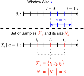
Figure 1: The parameter $s$ is the sliding window size of contexts $\theta_{t-s}$ to $\theta_{t-1}$ that are used for predicting the reward $X_{t}$. For example, if $s=3$, then at round $t$ the learner uses contexts $\theta_{t-3}$ to $\theta_{t-1}$ for predicting the reward $X_{t}$. The set $\mathscr{T}_{a}$ has all the rounds $t_{i}$ where action $a\in[k]$ is chosen and $N_{a}$ is the number of times action $a\in[k]$ that has been chosen by the learner. For example, if the learner choose action $a=1$ at rounds $t_{1}$, $t_{2}$ and $t_{3}$, then set $\mathscr{T}_{1}=\{t_{1},t_{2},t_{3}\}$ and $N_{1}=3$.

Remark 3.

We will control the parameters $N_{a}$ and $s$ separately in a hierarchical manner. We leave the study of their possible impacts on each other to future work.

IV-A Perturbation Method

Taking inspiration from [2], this subsection provides a way of controlling $N_{a}$ by using a perturbation signal $u_{a}$.

The learner chooses actions $a\in[k]$ with the highest reward prediction. Due to model error, the learner may constantly choose a sub-optimal action $a\in[k]$ without exploring other actions. To prevent this situation, a input signal $u_{a}\in\mathbb{R}$ is added such that the action the learner chooses is based on the following optimization problem

$$\max_{a\in[k]}\,\hat{G}_{a}\left(\mathscr{T}_{a},s\right)^{\top}\Theta_{t}+u_{a}.$$ (21)

We will design $u_{a}$ such that the regret is optimized. To understand how the signal $u_{a}$ impacts performance, we will consider the probability of choosing the optimal action $a_{t}^{*}$ using $u_{a}$; the following steps will be used for understanding the impact:
$\bullet$ STEP 1: Providing a bound on the model error $\left\|\hat{G}_{a}\left(\mathscr{T}_{a},s\right)-G_{a}\left(s\right)\right\|_{V_{a}\left(\mathscr{T}_{a},s\right)}$.
$\bullet$ STEP 2: Providing a bound on the error $\left|\hat{G}_{a}\left(\mathscr{T}_{a},s\right)^{\top}\Theta_{t}-G_{a}\left(s\right)^{\top}\Theta_{t}\right|$.
$\bullet$ STEP 3: Characterizing the impact of the proposed method on the probability of selecting the optimal action $a_{t}^{\ast}$.

IV-A1 STEP 1

To provide a bound on the model error $\left\|\hat{G}_{a}\left(\mathscr{T}_{a},s\right)-G_{a}\left(s\right)\right\|_{V_{a}\left(\mathscr{T}_{a},s\right)}$, first we need to provide a bound on $\left\|\mathbf{B}_{\mathscr{T}_{a}}\right\|$.

Lemma 1.

Let $\hat{G}_{a}\left(\mathscr{T}_{a},s\right)$ and $G_{a}\left(s\right)$ be as in (III) and (20), respectively. Then, there exists $\delta\in(0,1)$ such that $\mathbf{O}_{\mathscr{T}_{a}}\mathbf{B}_{\mathscr{T}_{a}}^{\top}$ satisfies the following inequality with a probability of at least $1-\delta$:

$$\left\|\mathbf{O}_{\mathscr{T}_{a}}\mathbf{B}_{\mathscr{T}_{a}}^{\top}\right\|_{V_{a}\left(\mathscr{T}_{a},s\right)^{-1}}\leq\\ \frac{\sqrt{N_{a}}B_{c}B_{R}}{\delta}\sqrt{\mbox{tr}\left(I-\lambda V_{a}\left(\mathscr{T}_{a},s\right)^{-1}\right)},$$ (22)

where $B_{c}$ and $B_{R}$ are as in Assumptions 4 and 5, respectively.

Proof.

According to (14), we have:

$$\left\|\mathbf{O}_{\mathscr{T}_{a}}\mathbf{B}_{\mathscr{T}_{a}}^{\top}\right\|_{V_{a}\left(\mathscr{T}_{a},s\right)^{-1}}= \left\|\sum_{t\in\mathscr{T}_{a}}\Theta_{t}\beta_{a;t}\right\|_{V_{a}\left(\mathscr{T}_{a},s\right)^{-1}}$$

$$= \left\|\sum_{t\in\mathscr{T}_{a}}V_{a}\left(\mathscr{T}_{a},s\right)^{-1/2}\Theta_{t}\beta_{a;t}\right\|_{2},$$ (23)

which according to the triangular inequality and Cauchy-Schwarz inequality implies that:

$$\left\|\mathbf{O}_{\mathscr{T}_{a}}\mathbf{B}_{\mathscr{T}_{a}}^{\top}\right\|_{V_{a}\left(\mathscr{T}_{a},s\right)^{-1}}\\ \leq\sum_{t\in\mathscr{T}_{a}}\left|\beta_{a;t}\right|\sqrt{\Theta_{t}^{\top}V_{a}\left(\mathscr{T}_{a},s\right)^{-1}\Theta_{t}}.$$ (24)

According to (12), Assumption 4, and Remark 2, $\left|\beta_{a;t}\right|$ can be upper-bounded as follows:

$$\left|\beta_{a;t}\right|\leq\left\|c_{a}\right\|_{2}\left\|(\Gamma-\Gamma KC_{\theta})^{s}\hat{z}_{t-s}\right\|_{2},$$ (25)

which according to Assumption 4 and Markov’s inequality [26], it can be shown that the following inequality holds with a probability of at least $1-\delta$:

$$\left|\beta_{a;t}\right|\leq B_{c}\frac{\mathbb{E}\left[\left\|(\Gamma-\Gamma KC_{\theta})^{s}\hat{z}_{t-s}\right\|_{2}\right]}{\delta}.$$ (26)

By using the Jensen’s inequality [27], it follows from (26) that:

$$\left|\beta_{a;t}\right| \leq B_{c}\frac{\sqrt{\mbox{tr}\left(\mathbb{E}\left[(\Gamma-\Gamma KC_{\theta})^{s}\hat{z}_{t}\hat{z}_{t}^{\top}\left((\Gamma-\Gamma KC_{\theta})^{s}\right)^{\top}\right]\right)}}{\delta}.$$ (27)

We know that:

$$\mathbb{E}\left[\hat{z}_{t}\hat{z}_{t}^{\top}\right]=(\Gamma-\Gamma KC_{\theta})^{s}\mathbb{E}\left[\hat{z}_{t-s}\hat{z}_{t-s}^{\top}\right]\left((\Gamma-\Gamma KC_{\theta})^{s}\right)^{\top}\\ +\sum_{\tau=1}^{s}(\Gamma-\Gamma KC_{\theta})^{s-\tau}\Gamma K\left(C_{\theta}PC_{\theta}^{\top}+R\right)\cdot\\ K^{\top}\Gamma^{\top}\left((\Gamma-\Gamma KC_{\theta})^{s-\tau}\right)^{\top},$$ (28)

which according to the fact that $C_{\theta}PC_{\theta}^{\top}+R\succ 0$, and since Kalman filter ensures that $\rho\left(\Gamma-\Gamma KC_{\theta}\right)<1$, we get:

$$\mbox{tr}\left((\Gamma-\Gamma KC_{\theta})^{s}\mathbb{E}\left[\hat{z}_{t-s}\hat{z}_{t-s}^{\top}\right]\left((\Gamma-\Gamma KC_{\theta})^{s}\right)^{\top}\right)\\ \leq\mbox{tr}\left(\mathbb{E}\left[\hat{z}_{t}\hat{z}_{t}^{\top}\right]\right)$$ (29)

Therefore, it follows from (27) that the following inequality holds with a probability of at least $1-\delta$:

$$\left|\beta_{a;t}\right|\leq B_{c}\frac{\sqrt{\mbox{tr}\left(\mathbb{E}\left[\hat{z}_{t}\hat{z}_{t}^{\top}\right]\right)}}{\delta}.$$ (30)

In what follows, we will provide a bound on $\mathbb{E}\left[\hat{z}_{t}\hat{z}_{t}^{\top}\right]$. Since $z_{t}=\hat{z}_{t}+e_{t}$, orthogonality principle [28] implies that $\mbox{tr}\left(\mathbb{E}\left[\hat{z}_{t}e_{t}^{\top}+e_{t}\hat{z}_{t}^{\top}\right]\right)=0$. Thus, we have:

$$\mathbb{E}\left[z_{t}z_{t}^{\top}\mid\mathscr{F}_{t-1}\right]= \mathbb{E}\left[\left(\hat{z}_{t}+e_{t}\right)\left(\hat{z}_{t}+e_{t}\right)^{\top}\mid\mathscr{F}_{t-1}\right]$$

$$= \mathbb{E}\left[\hat{z}_{t}\hat{z}_{t}^{\top}+\hat{z}_{t}e_{t}^{\top}+e_{t}\hat{z}_{t}^{\top}+e_{t}e_{t}^{\top}\mid\mathscr{F}_{t-1}\right]$$

$$= \mathbb{E}\left[\hat{z}_{t}\hat{z}_{t}^{\top}\mid\mathscr{F}_{t-1}\right]+\mathbb{E}\left[\hat{z}_{t}e_{t}^{\top}+e_{t}\hat{z}_{t}^{\top}\mid\mathscr{F}_{t-1}\right]$$

$$+\mathbb{E}\left[e_{t}e_{t}^{\top}\mid\mathscr{F}_{t-1}\right]$$

$$= \mathbb{E}\left[\hat{z}_{t}\hat{z}_{t}^{\top}\mid\mathscr{F}_{t-1}\right]+\mathbb{E}\left[e_{t}e_{t}^{\top}\mid\mathscr{F}_{t-1}\right],$$ (31)

which implies that $\mathbb{E}\left[\mathbb{E}\left[z_{t}z_{t}^{\top}\mid\mathscr{F}_{t-1}\right]\right]=\hat{Z}_{t}+P_{t}$, where $\hat{Z}_{t}\triangleq\mathbb{E}\left[\hat{z}_{t}\hat{z}_{t}^{\top}\right]$ and $P_{t}\triangleq\mathbb{E}\left[e_{t}e_{t}^{\top}\mid\mathscr{F}_{t-1}\right]$. Since $\hat{Z}_{t}\succeq 0$ and $P_{t}\succeq 0$, and according to Assumption 5, it can be easily shown that

$$\sqrt{\mbox{tr}\left(\hat{Z}_{t}\right)}\leq\sqrt{\mbox{tr}\left(Z_{t}\right)}\leq B_{R}.$$ (32)

Thus, since the state of system (1) is bounded by $B_{R}$ according to Assumption 5, (30) and (32) imply that the following inequality holds with a probability of at least $1-\delta$:

$$\left|\beta_{a;t}\right|\leq\frac{B_{c}B_{R}}{\delta}.$$ (33)

Regarding the term $\sqrt{\Theta_{t}^{\top}V_{a}\left(\mathscr{T}_{a},s\right)^{-1}\Theta_{t}}$ in (24), we have:

$$\left\|\mathbf{O}_{\mathscr{T}_{a}}\mathbf{B}_{\mathscr{T}_{a}}^{\top}\right\|_{V_{a}\left(\mathscr{T}_{a},s\right)^{-1}}$$

$$~{}~{}\leq\sum_{t\in\mathscr{T}_{a}}\frac{B_{c}B_{R}}{\delta}\sqrt{\mbox{tr}\left(V_{a}\left(\mathscr{T}_{a},s\right)^{-1}\Theta_{t}\Theta_{t}^{\top}\right)\cdot 1}$$

$$~{}~{}\overset{(*)}{\leq}\frac{B_{c}B_{R}}{\delta}\sqrt{\sum_{t\in\mathscr{T}_{a}}\mbox{tr}\left(V_{a}\left(\mathscr{T}_{a},s\right)^{-1}\Theta_{t}\Theta_{t}^{\top}\right)}\cdot\sqrt{\sum_{t\in\mathscr{T}_{a}}1}$$

$$~{}~{}\leq\sqrt{N_{a}}\frac{B_{c}B_{R}}{\delta}\sqrt{\sum_{t\in\mathscr{T}_{a}}\mbox{tr}\left(V_{a}\left(\mathscr{T}_{a},s\right)^{-1}\Theta_{t}\Theta_{t}^{\top}\right)}$$

$$~{}~{}\leq\sqrt{N_{a}}\frac{B_{c}B_{R}}{\delta}\sqrt{\mbox{tr}\left(V_{a}\left(\mathscr{T}_{a},s\right)^{-1}\sum_{t\in\mathscr{T}_{a}}\Theta_{t}\Theta_{t}^{\top}\right)},$$ (34)

where $(*)$ is concluded based on the Cauchy-Schwarz inequality. Since $\sum_{\tau\in\mathscr{T}_{a}}\Theta_{\tau}\Theta_{\tau}^{\top}=V_{a}\left(\mathscr{T}_{a},s\right)-\lambda I$, we can rewrite (IV-A1) as follows:

$$\left\|\mathbf{O}_{\mathscr{T}_{a}}\mathbf{B}_{\mathscr{T}_{a}}^{\top}\right\|_{V_{a}\left(\mathscr{T}_{a},s\right)^{-1}}$$

$$~{}~{}~{}~{}\leq\sqrt{N_{a}}\frac{B_{c}B_{R}}{\delta}\sqrt{\mbox{tr}\left(V_{a}\left(\mathscr{T}_{a},s\right)^{-1}\left(V_{a}\left(\mathscr{T}_{a},s\right)-\lambda I\right)\right)}.$$ (35)

Note that the matrix $\sum_{\tau\in\mathscr{T}_{a}}\Theta_{\tau}\Theta_{\tau}^{\top}\succeq 0$, implying that $V_{a}\left(\mathscr{T}_{a},s\right)\succeq\lambda I$. Thus, the terms in the square root of inequality (35) is always non-negative. According to (33) and (35), no further effort is needed to show that inequality (22) is satisfied with a probability of at least $1-\delta$. ∎

Using Lemma 1, the following theorem completes STEP 1.

Theorem 1.

Let $\hat{G}_{a}\left(\mathscr{T}_{a},s\right)$ be identified as in (20) and the reward $\mathbf{X}_{\mathscr{T}_{a}}$ is as in (14). Then, there exists $\delta\in(0,1)$ such that the following inequality is satisfied with a probability of at least $(1-\delta)^{2}$:

$$\left\|\hat{G}_{a}\left(\mathscr{T}_{a},s\right)-G_{a}\left(s\right)\right\|_{V_{a}\left(\mathscr{T}_{a},s\right)}\leq b_{a}\left(\delta,s\right),$$

where

$$b_{a}\left(\delta,s\right)\triangleq \sqrt{2B_{R}^{2}\log\left(\frac{1}{\delta}\frac{\det(V_{a}\left(\mathscr{T}_{a},s\right))^{1/2}}{\det(\lambda I)^{1/2}}\right)}$$

$$+\frac{\sqrt{N_{a}}B_{c}B_{R}}{\delta}\sqrt{\mbox{tr}\left(I-\lambda V_{a}\left(\mathscr{T}_{a},s\right)^{-1}\right)}$$

$$+\lambda B_{G}\sqrt{\mbox{tr}\left(V_{a}\left(\mathscr{T}_{a},s\right)^{-1}\right)}.$$ (36)

Proof.

From (14) and (20), we have:

$$\hat{G}_{a}\left(\mathscr{T}_{a},s\right)^{\top}= G_{a}\left(s\right)^{\top}\mathbf{O}_{\mathscr{T}_{a}}\mathbf{O}_{\mathscr{T}_{a}}^{\top}V_{a}\left(\mathscr{T}_{a},s\right)^{-1}$$

$$+\left(\mathbf{B}_{\mathscr{T}_{a}}+\mathbf{E}_{\mathscr{T}_{a}}\right)\mathbf{O}_{\mathscr{T}_{a}}^{\top}V_{a}\left(\mathscr{T}_{a},s\right)^{-1}.$$ (37)

Adding and subtracting the term $\lambda G_{a}\left(s\right)^{\top}V_{a}\left(\mathscr{T}_{a},s\right)^{-1}$ from the right-hand side of (37) yields:

$$\hat{G}_{a}\left(\mathscr{T}_{a},s\right)^{\top}= G_{a}\left(s\right)^{\top}\left(\mathbf{O}_{\mathscr{T}_{a}}\mathbf{O}_{\mathscr{T}_{a}}^{\top}+\lambda I\right)V_{a}\left(\mathscr{T}_{a},s\right)^{-1}$$

$$+\left(\mathbf{B}_{\mathscr{T}_{a}}+\mathbf{E}_{\mathscr{T}_{a}}\right)\mathbf{O}_{\mathscr{T}_{a}}^{\top}V_{a}\left(\mathscr{T}_{a},s\right)^{-1}$$

$$-\lambda G_{a}\left(s\right)^{\top}V_{a}\left(\mathscr{T}_{a},s\right)^{-1},$$

which according to the fact that $V_{a}\left(\mathscr{T}_{a},s\right)=\lambda I+\mathbf{O}_{\mathscr{T}_{a}}\mathbf{O}_{\mathscr{T}_{a}}^{\top}$, implies that:

$$\hat{G}_{a}\left(\mathscr{T}_{a},s\right)^{\top}-G_{a}\left(s\right)^{\top}= -\lambda G_{a}\left(s\right)^{\top}V_{a}\left(\mathscr{T}_{a},s\right)^{-1}$$

$$+\left(\mathbf{B}_{\mathscr{T}_{a}}+\mathbf{E}_{\mathscr{T}_{a}}\right)\mathbf{O}_{\mathscr{T}_{a}}^{\top}V_{a}\left(\mathscr{T}_{a},s\right)^{-1}.$$ (38)

Multiplying both sides of this last equation by $V_{a}\left(\mathscr{T}_{a},s\right)$ from right yields:

$$\Big{(}\hat{G}_{a} \left(\mathscr{T}_{a},s\right)-G_{a}\left(s\right)\Big{)}^{\top}V_{a}\left(\mathscr{T}_{a},s\right)$$

$$= \left(-\lambda G_{a}\left(s\right)+\mathbf{O}_{\mathscr{T}_{a}}\left(\mathbf{B}_{\mathscr{T}_{a}}+\mathbf{E}_{\mathscr{T}_{a}}\right)^{\top}\right)^{\top}.$$ (39)

Multiplying the right- and left-hand sides of (38) by transpose of the right- and left-hand sides of (38), respectively, and according to the fact that $V_{a}\left(\mathscr{T}_{a},s\right)^{-1}=\left(V_{a}\left(\mathscr{T}_{a},s\right)^{-1}\right)^{\top}$, we obtain the following:

$$\Big{\|}\hat{G}_{a} \left(\mathscr{T}_{a},s\right)-G_{a}\left(s\right)\Big{\|}_{V_{a}\left(\mathscr{T}_{a},s\right)}$$

$$= \left\|-\lambda G_{a}\left(s\right)+\mathbf{O}_{\mathscr{T}_{a}}\left(\mathbf{B}_{\mathscr{T}_{a}}+\mathbf{E}_{\mathscr{T}_{a}}\right)^{\top}\right\|_{V_{a}\left(\mathscr{T}_{a},s\right)^{-1}}.$$ (40)

Using the triangle inequality, it follows from (IV-A1) that:

$$\left\|\hat{G}_{a}\left(\mathscr{T}_{a},s\right)-G_{a}\left(s\right)\right\|_{V_{a}\left(\mathscr{T}_{a},s\right)}\leq\left\|\lambda G_{a}\left(s\right)\right\|_{V_{a}\left(\mathscr{T}_{a},s\right)^{-1}}\\ +\left\|\mathbf{O}_{\mathscr{T}_{a}}\mathbf{B}_{\mathscr{T}_{a}}^{\top}\right\|_{V_{a}\left(\mathscr{T}_{a},s\right)^{-1}}+\left\|\mathbf{O}_{\mathscr{T}_{a}}\mathbf{E}_{\mathscr{T}_{a}}^{\top}\right\|_{V_{a}\left(\mathscr{T}_{a},s\right)^{-1}}.$$ (41)

Since $\varepsilon_{a;\tau}$ is conditionally $B_{R}$-sub-Gaussian on $\mathscr{F}_{t-1}$ and $\Theta_{t}$ is $\mathscr{F}_{t-1}$ measurable, it can be concluded that [25, Theorem 1] there exists $\delta\in(0,1)$ such that the following inequality is satisfied with a probability of at least $1-\delta$:

$$\left\|\mathbf{O}_{\mathscr{T}_{a}}\mathbf{E}_{\mathscr{T}_{a}}^{\top}\right\|_{V_{a}\left(\mathscr{T}_{a},s\right)^{-1}}\leq\\ \sqrt{2B_{R}^{2}\log\left(\frac{1}{\delta}\frac{\det(V_{a}\left(\mathscr{T}_{a},s\right))^{1/2}}{\det(\lambda I)^{1/2}}\right)}.$$ (42)

Finally, according to Assumption 3, we have:

$$\left\|\lambda G_{a}\left(s\right)\right\|_{V_{a}\left(\mathscr{T}_{a},s\right)^{-1}} \leq\lambda\left\|V_{a}\left(\mathscr{T}_{a},s\right)^{-1}\right\|_{2}\left\|G_{a}\left(s\right)\right\|_{2}$$

$$\leq B_{G}\lambda\sqrt{\mbox{tr}\left(V_{a}\left(\mathscr{T}_{a},s\right)^{-1}\right)}.$$ (43)

Thus, from Lemma 1, and according to inequalities (42) and (IV-A1), one can obtain the bound given in (1), which completes the proof. ∎

IV-A2 STEP 2

Using results from STEP 1, the following lemma will complete STEP 2.

Lemma 2.

There exists $\delta\in(0,1)$ such that the following inequality holds with a probability of at least $(1-\delta)^{2}$:

$$\left|\hat{G}_{a}\left(\mathscr{T}_{a},s\right)^{\top}\Theta_{t}-G_{a}\left(s\right)^{\top}\Theta_{t}\right|$$

$$~{}~{}~{}~{}~{}~{}~{}~{}~{}~{}~{}\leq b_{a}\left(\delta,s\right)\sqrt{\Theta_{t}^{\top}V_{a}\left(\mathscr{T}_{a},s\right)^{-1}\Theta_{t}}.$$ (44)

Proof.

Consider the following optimization problem

$$\begin{array}[]{cc}\underset{\tilde{G}\in\mathbb{R}^{(ms+1)\times 1}}{\max}&\tilde{G}^{\top}\Theta_{t}\\ \mbox{ s.t. }&\tilde{G}\in\mathscr{C}_{a,s}\end{array},$$ (45)

where the set $\mathscr{C}_{a,s}$ is defined as follows:

$$\mathscr{C}_{a,s}=\left\{\tilde{G}\big{|}\|\hat{G}_{a}\left(\mathscr{T}_{a},s\right)-\tilde{G}\|_{V_{a}\left(\mathscr{T}_{a},s\right)}\leq b_{a}(\delta,s)\right\},$$ (46)

with $b_{a}\left(\delta,s\right)$ as in (1). The Lagrangian $L(\tilde{G},\nu)$ for optimization problem (45) is

$$L(\tilde{G},\nu)=\tilde{G}^{\top}\Theta_{t}\\ -\nu\left(\left\|\hat{G}_{a}\left(\mathscr{T}_{a},s\right)-\tilde{G}\right\|_{V_{a}\left(\mathscr{T}_{a},s\right)}^{2}-b_{a}\left(\delta,s\right)^{2}\right),$$ (47)

where $\nu$ is Lagrange multiplier. The partial derivatives of $L(\tilde{G},\nu)$ are

$$\frac{\partial L(\cdot)}{\partial\tilde{G}^{\top}}=\Theta_{t}^{\top}-2\nu\tilde{G}^{\top}V_{a}\left(\mathscr{T}_{a},s\right)+2\nu\hat{G}_{a}\left(\mathscr{T}_{a},s\right)^{\top}V_{a}\left(\mathscr{T}_{a},s\right),$$

and

$$\frac{\partial L(\cdot)}{\partial\mu}=-\left\|\hat{G}_{a}\left(\mathscr{T}_{a},s\right)-\tilde{G}\right\|_{V_{a}\left(\mathscr{T}_{a},s\right)}^{2}+b_{a}\left(\delta,s\right)^{2}.$$ (48)

Solving $\partial L(\tilde{G},\nu)/\partial\tilde{G}^{\top}=0$ for $\tilde{G}$ yields

$$\Theta_{t}^{\top}-2\nu\tilde{G}^{\top}V_{a}\left(\mathscr{T}_{a},s\right)+2\nu\hat{G}_{a}\left(\mathscr{T}_{a},s\right)^{\top}V_{a}\left(\mathscr{T}_{a},s\right)=0,$$ (49)

which implies that

$$\tilde{G}^{\top}=\hat{G}_{a}\left(\mathscr{T}_{a},s\right)^{\top}+\frac{\Theta_{t}^{\top}V_{a}\left(\mathscr{T}_{a},s\right)^{-1}}{2\nu}.$$ (50)

Using $\tilde{G}$ given in (50) in (48), and solving $\partial L(\tilde{G},\nu)/\partial\nu=0$ for $\nu$ yields:

$$\nu=\frac{\sqrt{\Theta_{t}^{\top}V_{a}\left(\mathscr{T}_{a},s\right)^{-1}\Theta_{t}}}{2b_{a}\left(\delta,s\right)}.$$ (51)

Plugging the obtained $\nu$ in (50) yields

$$\tilde{G}^{\top} =\hat{G}_{a}\left(\mathscr{T}_{a},s\right)^{\top}+\frac{\Theta_{t}^{\top}V_{a}\left(\mathscr{T}_{a},s\right)^{-1}}{2\nu}$$

$$=\hat{G}_{a}\left(\mathscr{T}_{a},s\right)^{\top}$$

$$~{}~{}~{}~{}~{}~{}~{}~{}+\frac{\Theta_{t}^{\top}V_{a}\left(\mathscr{T}_{a},s\right)^{-1}}{2}\left(\frac{\sqrt{\Theta_{t}^{\top}V_{a}\left(\mathscr{T}_{a},s\right)^{-1}\Theta_{t}}}{2b_{a}\left(\delta,s\right)}\right)^{-1},$$ (52)

which is the solution of the optimization problem (45). Since this optimal value lies on the edge of the confidence interval $\mathscr{C}_{a,s}$ given in (46), then with a probability of at least $(1-\delta)^{2}$, we have

$$G_{a}\left(s\right)^{\top}\Theta_{t}\leq\hat{G}_{a}\left(\mathscr{T}_{a},s\right)^{\top}\Theta_{t}\\ +b_{a}\left(\delta,s\right)\sqrt{\Theta_{t}^{\top}V_{a}\left(\mathscr{T}_{a},s\right)^{-1}\Theta_{t}},$$ (53)

which yields the inequality (2) and completes the proof. ∎

IV-A3 STEP 3

Finally, since STEP 1 and STEP 2 have been proven, we can now design the perturbation signal $u_{a}$. To provide the performance of using the proposed $u_{a}$, the following theorem explains perturbation signal’s impact on selecting the optimal action $a_{t}$.

Theorem 2.

Let $r_{t}:=G_{a^{*}}(s)^{\top}\Theta_{t}-G_{a}(s)^{\top}\Theta_{t}$ be instantaneous pseudo-regret, where $a^{\ast}$ is the optimal action at round $t$. Then, if $u_{a}$ in (21) is selected as

$$u_{a}=b_{a}\left(\delta,s\right)\sqrt{\Theta_{t}^{\top}V_{a}\left(\mathscr{T}_{a},s\right)^{-1}\Theta_{t}},$$ (54)

the following inequality holds with a probability of at least $(1-\delta)^{4}$:

$$r_{t}\leq 2b_{a}\left(\delta,s\right)\sqrt{\Theta_{t}^{\top}V_{a}\left(\mathscr{T}_{a},s\right)^{-1}\Theta_{t}},$$ (55)

where $b_{a}\left(\delta,s\right)$ is as in (1).

Proof.

Assume that action $a$ is chosen based on the following optimization problem

$$a=\underset{a\in[k]}{\arg\max}~{}\hat{G}_{a}\left(\mathscr{T}_{a},s\right)^{\top}\Theta_{t}+u_{a},$$ (56)

where $u_{a}\in\mathbb{R}$ is a perturbation term to be defined later. Using Lemma 2, instantaneous pseudo-regret $r_{t}$ has the following upper bound with a probability of at least $(1-\delta)^{2}$:

$$r_{t}\leq\hat{G}_{a^{*}}\left(\mathscr{T}_{a^{*}},s\right)^{\top}\Theta_{t}-G_{a}(s)^{\top}\Theta_{t}$$

$$~{}~{}~{}~{}~{}~{}~{}~{}~{}~{}~{}~{}~{}~{}~{}~{}~{}~{}~{}~{}~{}+b_{a}\left(\delta,s\right)\sqrt{\Theta_{t}^{\top}V_{a}\left(\mathscr{T}_{a},s\right)^{-1}\Theta_{t}}.$$ (57)

From optimality, the obtained action $a\in[k]$ from the optimization problem (56) satisfies the following inequality:

$$\hat{G}_{a}\left(\mathscr{T}_{a},s\right)^{\top}\Theta_{t}+u_{a}\geq\hat{G}_{a^{*}}\left(\mathscr{T}_{a^{\ast}},s\right)^{\top}\Theta_{t}+u_{a^{\ast}}.$$ (58)

According to (IV-A3) and (58), it can be concluded that $r_{t}$ satisfies the following inequality with a probability of at least $(1-\delta)^{4}$:

$$r_{t}\leq b_{a}\left(\delta,s\right)\sqrt{\Theta_{t}^{\top}V_{a}\left(\mathscr{T}_{a},s\right)^{-1}\Theta_{t}}$$

$$+b_{a^{\ast}}\left(\delta,s\right)\sqrt{\Theta_{t}^{\top}V_{a^{\ast}}\left(\mathscr{T}_{a^{\ast}},s\right)^{-1}\Theta_{t}}+u_{a}-u_{a^{\ast}}.$$ (59)

At this stage, let us define $u_{a}$ as in (54); note that in this case, we have $u_{a^{\ast}}=b_{a^{\ast}}\left(\delta,s\right)\sqrt{\Theta_{t}^{\top}V_{a^{\ast}}\left(\mathscr{T}_{a^{\ast}},s\right)^{-1}\Theta_{t}}$. Therefore, according to (IV-A3), no further effort is needed to show that inequality (55) is satisfied with a probability of at least $(1-\delta)^{4}$, which competes the proof. ∎

IV-B Adaptive Window-Size

As mentioned in Remark 2, the window-size parameter $s$ impacts the magnitude of the bias term $\beta_{a;t}$. Also, according to Theorem 1 and Lemma 2, the window-size parameter $s$ impacts the model error $\left\|\hat{G}_{a}\left(\mathscr{T}_{a},s\right)-G_{a}\left(s\right)\right\|_{V_{a}\left(\mathscr{T}_{a},s\right)}$ (and consequently, the error $\hat{G}_{a}\left(\mathscr{T}_{a},s\right)^{\top}\Theta_{t}-G_{a}\left(s\right)^{\top}\Theta_{t}$). The following theorem provides a method to adaptively control the parameter $s$ so as to minimize the impact of the bias term and the model error on the model $\hat{G}_{a}\left(\mathscr{T}_{a},s\right)$ that predicts the reward $X_{t}$.

Theorem 3.

Let $J_{a}[\mathscr{T}_{a},s]$ be a cost function defined as:

$$J_{a}[\mathscr{T}_{a},s]:=\left|X_{t}-\hat{G}_{a}\left(\mathscr{T}_{a},s\right)^{\top}\Theta_{t}\right|\\ +b_{a}\left(\delta,s\right)\sqrt{\Theta_{t}^{\top}V_{a}\left(\mathscr{T}_{a},s\right)^{-1}\Theta_{t}}.$$ (60)

Then, there exists $\delta\in(0,1)$ such that the following inequality is satisfied with a probability of at least $(1-\delta)^{2}$:

$$J_{a}[\mathscr{T}_{a},s]+\left|\varepsilon_{a;t}\right|\geq \left|\beta_{a;t}\right|.$$ (61)

Proof.

Subtracting $\hat{G}_{a}\left(\mathscr{T}_{a},s\right)^{\top}\Theta_{t}$ and $\varepsilon_{a;t}$ from both sides of model (11) yields:

$$X_{t}- \hat{G}_{a}\left(\mathscr{T}_{a},s\right)^{\top}\Theta_{t}-\varepsilon_{a;t}=$$

$$G_{a}\left(s\right)^{\top}\Theta_{t}-\hat{G}_{a}\left(\mathscr{T}_{a},s\right)^{\top}\Theta_{t}+\beta_{a;t},$$ (62)

Rearranging the terms provides

$$X_{t}-\hat{G}_{a}\left(\mathscr{T}_{a},s\right)^{\top}\Theta_{t}-\varepsilon_{a;t}\\ -G_{a}\left(s\right)^{\top}\Theta_{t}+\hat{G}_{a}\left(\mathscr{T}_{a},s\right)^{\top}\Theta_{t}=\beta_{a;t},$$ (63)

which according to the triangle inequality implies that:

$$\left|\beta_{a;t}\right|\leq\left|X_{t}-\hat{G}_{a}\left(\mathscr{T}_{a},s\right)^{\top}\Theta_{t}\right|\\ +\left|G_{a}\left(s\right)^{\top}\Theta_{t}-\hat{G}_{a}\left(\mathscr{T}_{a},s\right)^{\top}\Theta_{t}\right|+\left|\varepsilon_{a;t}\right|$$ (64)

According to Lemma 2, it follows from (64) that the following inequality is satisfied with a probability of at least $(1-\delta)^{2}$:

$$\left|\beta_{a;t}\right|\leq\left|X_{t}-\hat{G}_{a}\left(\mathscr{T}_{a},s\right)^{\top}\Theta_{t}\right|\\ +b_{a}\left(\delta,s\right)\sqrt{\Theta_{t}^{\top}V_{a}\left(\mathscr{T}_{a},s\right)^{-1}\Theta_{t}}+\left|\varepsilon_{a;t}\right|$$ (65)

Therefore, no further effort is need to prove that the inequality (61) is satisfied with the probability of at least $(1-\delta)^{2}$; this completes the proof. ∎

Remark 4.

According to the fact that $\varepsilon_{a;t}$ is invariant to $s$, Theorem 3 suggests that minimizing the cost function $J_{a}[\mathscr{T}_{a},s]$ would minimize the bias term $\beta_{a;t}$.

V Bandit Strategy

The strategy the learner will use when choosing an action $a\in[k]$ is based on the theorems and lemmas mentioned above which can be broken down into two parts: Part 1: selecting parameter $s$ and Part 2: selecting action $a\in[k]$. This is comprehensively shown in Algorithm 1. Fig. 2 illustrates Part 1 and Part 2 of the algorithm.

Part 1: A model $\hat{G}_{a}\left(\mathscr{T}_{a},s\right)\leftarrow\mathbf{0}_{(ms+1)\times 1}$ is set for each parameter $s\in\mathscr{S}\triangleq\{0,1,\dots,s_{N}\}$ and action $a\in[k]$, where $s_{N}$ is a preset value for the maximum window size of previous observations that are used. This provides $s_{N}\times k$ models. For each parameter $s\in\mathscr{S}\triangleq\{0,1,\dots,s_{N}\}$ and action $a\in[k]$, the cost function $J_{a}[\mathscr{T}_{a},s]$ is computed. Model $\hat{G}_{a}\left(\mathscr{T}_{a},s\right)$ and perturbation term $u_{a}$ use parameter $s_{a}$ that minimizes $J_{a}[\mathscr{T}_{a},s]$, i.e. $s_{a}=\arg\min_{s\in\{0,1,\dots,s_{N}\}}J_{a}[\mathscr{T}_{a},s]$.

Part 2: The action $a\in[k]$ that the learner chooses is $a=\arg\max_{a\in[k]}\hat{G}_{a}\left(\mathscr{T}_{a},s\right)^{\top}\Theta_{t}+u_{a}$, where $u_{a}$ is defined in (54).

Algorithm 1 Adaptive Recursive least-squares Exploration of System (ARES)

Input: $\delta,\delta\in(0,1)$, $k$, $s_{N}$, $\lambda$

1:  $t\leftarrow 1$

2:  $\mathscr{S}=\{0,1,\dots,s_{N}\}$

3:  for $a\in[k]$ do

4:     $\mathscr{T}_{a}\leftarrow\{\}$

5:     for $s=\{0,1,\dots,s_{N}\}$ do

6:        $M_{a}\leftarrow 0$

7:        $N_{a}\leftarrow 0$

8:        $V_{a}\leftarrow\lambda I_{ms+1\times ms+1}$

9:        $\hat{G}_{a}\left(\mathscr{T}_{a},s\right)\leftarrow\mathbf{0}_{(ms+1)\times 1}$

10:        $b_{a}\left(\delta,s\right)\leftarrow 1/\epsilon$ where $\epsilon$ small

11:        $J_{a}[\mathscr{T}_{a},s]=0$

12:     end for

13:  end for

14:  for $t\in[n]$ do

15:     for $a\in[k]$ do

16:        $s_{a}\leftarrow\underset{s\in\{0,1,\dots,s_{N}\}}{\arg\min}J_{a}[\mathscr{T}_{a},s]$

17:        $u_{a}\leftarrow\begin{cases}b_{a}\left(\delta,s\right)\sqrt{\Theta_{t}^{\top}V_{a}\left(\mathscr{T}_{a},s\right)^{-1}\Theta_{t}}&\mbox{ if }t\geq s_{a}\\ \sqrt{2\frac{\log(1/\delta)}{M_{a}}}&\mbox{ if }t<s_{a}\end{cases}$

18:     end for

19:     $a^{*}\leftarrow\underset{a\in\{1,2,\dots,k\}}{\arg\max}\begin{cases}\hat{G}_{a}\left(\mathscr{T}_{a},s_{a}\right)^{\top}\Theta_{t}+u_{a}&\mbox{ if }t\geq s_{a}\\ \sum_{t\in\mathscr{T}_{a}}\frac{X_{t}}{M_{a}}+u_{a}&\mbox{ if }t<s_{a}\end{cases}$

20:     Sample $(X_{t},\theta_{t})$ from (1)

21:     $\mathscr{T}_{a^{*}}\leftarrow\mathscr{T}_{a^{*}}\cup\{t\}$

22:     $M_{a^{*}}\leftarrow M_{a^{*}}+1$ if $t<s_{a^{*}}$

23:     $N_{a^{*}}\leftarrow N_{a^{*}}+1$ if $t\geq s_{a^{*}}$

24:     for $s\in\{0,1,\dots,\min(t,s_{N})\}$ do

25:        $V_{a^{*}}\left(\mathscr{T}_{a^{*}},s\right)\leftarrow V_{a^{*}}\left(\mathscr{T}_{a^{*}},s\right)+\Theta_{\tau}\Theta_{\tau}^{\top}$

26:        $\hat{G}_{a^{*}}\left(\mathscr{T}_{a^{*}},s\right)^{\top}\leftarrow\hat{G}_{a^{*}}\left(\mathscr{T}_{a^{*}},s\right)^{\top}$ $+X_{\tau}\Theta_{\tau}^{\top}V_{a^{*}}\left(\mathscr{T}_{a^{*}},s\right)^{-1}$

27:        Update $b_{a^{*}}(\delta,s)$ based on (1)

28:     end for

29:  end for

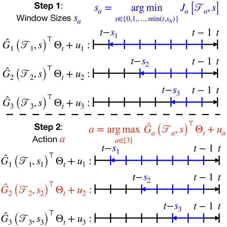
Figure 2: In step 1, the learner selects the window size $s_{a}$ for each action $a\in[k]$. As for step 2, the learner selects the action $a\in[k]$ that maximizes the quantity $\hat{G}_{a}\left(\mathscr{T}_{a},s_{a}\right)^{\top}\Theta_{t}+u_{a}$ with the chosen $s_{a}$.

VI Regret Analysis of the Proposed Algorithm

The following theorem provides a bound for regret given in (2) if Algorithm 1 is used to determine the actions.

Theorem 4.

Let $s\equiv s_{N}$. Regret $\sum_{t=1}^{n}X_{t}^{*}-X_{t}$ has the following bound with a probability of at least $(1-\delta)^{5}$:

$$R_{n}\leq 2knB_{a}\left(\delta,s\right)\sqrt{\frac{ms+1}{\lambda}}\frac{M_{\theta}}{\delta}+2kn\frac{B_{c}B_{R}}{\delta}\\ +kn\sqrt{4B_{R}^{2}\log(1/\delta)},$$ (66)

where $B_{a}(\delta,s)$ and $M_{\Theta}$ are defined as

$$B_{a}\left(\delta,s\right)\triangleq\\ \Bigg{(}2B_{R}^{2}\left(\log(1/\delta)+\frac{ms+1}{2}\log\left(\frac{\mbox{tr}\left(\lambda I_{ms+1}\right)+n\frac{M_{\theta}^{2}}{\delta}}{ms+1}\right)\right)\\ -2B_{R}^{2}\left(\frac{1}{2}\log\det\left(\lambda I_{ms+1}\right)\right)\Bigg{)}^{1/2}\\ +\frac{\sqrt{n}B_{c}B_{R}}{\delta}\sqrt{ms+1}+\lambda B_{G}\sqrt{\frac{ms+1}{\lambda}},$$ (67)

and

$$M_{\Theta}\triangleq\max_{t\in[n]}\mathbb{E}\left[\sqrt{\Theta_{t}^{\top}\Theta_{t}}\right].$$ (68)

Proof.

According to (11), instantaneous regret $r_{t}\triangleq X_{t}^{*}-X_{t}$ has the following upper bound

$$r_{t}= X_{t}^{\ast}-X_{t}$$

$$= G_{a^{*}}\left(s\right)^{\top}\Theta_{t}-G_{a}\left(s\right)^{\top}\Theta_{t}+\beta_{a^{*};t}-\beta_{a;t}+\varepsilon_{a^{*};t}-\varepsilon_{a;t}.$$ (69)

On the one hand, based on Lemma 2, with a probability of at least $(1-\delta)^{2}$, the following inequality is satisfied:

$$G_{a^{*}}\left(s\right)^{\top}\Theta_{t}\leq \hat{G}_{a^{*}}\left(s\right)^{\top}\Theta_{t}$$

$$+b_{a^{*}}\left(\delta,s\right)\sqrt{\Theta_{t}^{\top}V_{a^{*}}\left(\mathscr{T}_{a^{*}},s\right)^{-1}\Theta_{t}}.$$ (70)

On the other hand, action $a$ is chosen because of the following relationship

$$\hat{G}_{a^{*}}\left(s\right)^{\top}\Theta_{t} +b_{a^{*}}\left(\delta,s\right)\sqrt{\Theta_{t}^{\top}V_{a^{*}}\left(\mathscr{T}_{a^{*}},s\right)^{-1}\Theta_{t}}\leq$$

$$\hat{G}_{a}\left(s\right)^{\top}\Theta_{t}+b_{a}\left(\delta,s\right)\sqrt{\Theta_{t}^{\top}V_{a}\left(\mathscr{T}_{a},s\right)^{-1}\Theta_{t}}.$$ (71)

Therefore, inequality (69) can be upper-bounded by

$$r_{t}\leq\hat{G}_{a}\left(s\right)^{\top}\Theta_{t}+b_{a}\left(\delta,s\right)\sqrt{\Theta_{t}^{\top}V_{a}\left(\mathscr{T}_{a},s\right)^{-1}\Theta_{t}}\\ -G_{a}\left(s\right)^{\top}\Theta_{t}+\beta_{a^{*};t}-\beta_{a;t}+\varepsilon_{a^{*};t}-\varepsilon_{a;t}.$$ (72)

By Lemma 1, the difference $\hat{G}_{a}\left(s\right)^{\top}\Theta_{t}-G_{a}\left(s\right)^{\top}\Theta_{t}$ has the following upper bound with a probability of at least $(1-\delta)^{2}$

$$\hat{G}_{a}\left(s\right)^{\top}\Theta_{t}-G_{a}\left(s\right)^{\top}\Theta_{t}\leq b_{a}\left(\delta,s\right)\sqrt{\Theta_{t}^{\top}V_{a}\left(\mathscr{T}_{a},s\right)^{-1}\Theta_{t}},$$

adjusting bound (72) to be

$$r_{t}\leq 2b_{a}\left(\delta,s\right)\sqrt{\Theta_{t}^{\top}V_{a}\left(\mathscr{T}_{a},s\right)^{-1}\Theta_{t}}+\beta_{a^{*};t}-\beta_{a;t}+\varepsilon_{a^{*};t}-\varepsilon_{a;t}.$$

To upper bound the term $b_{a}\left(\delta,s\right)\sqrt{\Theta_{t}^{\top}V_{a}\left(\mathscr{T}_{a},s\right)^{-1}\Theta_{t}}$, first we show that $b_{a}\left(\delta,s\right)\leq B_{a}(\delta,s)$ with a probability of at least $(1-\delta)^{2}$, where $B_{a}(\delta,s)$ is as in (67):

• First term in $b_{a}\left(\delta,s\right)$: Since $\left\|\Theta_{t}\right\|_{2}\leq\frac{M_{\theta}}{\delta}$ with a probability of at least $1-\delta$, Lemma 11 of [25] implies that:

  $$\sqrt{2B_{R}^{2}\log\left(\frac{1}{\delta}\frac{\det(V_{a}\left(\mathscr{T}_{a},s\right))^{1/2}}{\det(\lambda I)^{1/2}}\right)}\leq\Bigg{(}2B_{R}^{2}\bigg{(}\log(1/\delta)$$

  $$+\frac{ms+1}{2}\log\bigg{(}\frac{\mbox{tr}\left(\lambda I_{ms+1}\right)+n\frac{M_{\theta}^{2}}{\delta}}{ms+1}\bigg{)}\bigg{)}$$

  $$-2B_{R}^{2}\left(\frac{1}{2}\log\det\left(\lambda I_{ms+1}\right)\right)\Bigg{)}^{1/2};$$ (73)

• Second term in $b_{a}\left(\delta,s\right)$: Since $V_{a}\left(\mathscr{T}_{a},s\right)\succ 0$ implying that $-\lambda V_{a}\left(\mathscr{T}_{a},s\right)^{-1}\prec 0$, the following upper-bound can be obtained

  $$\frac{\sqrt{N_{a}}B_{c}B_{R}}{\delta}\sqrt{\mbox{tr}\left(I-\lambda V_{a}\left(\mathscr{T}_{a},s\right)^{-1}\right)}\leq$$

  $$~{}~{}~{}~{}~{}~{}~{}~{}~{}~{}~{}~{}~{}~{}~{}~{}~{}~{}~{}~{}~{}~{}~{}~{}~{}~{}~{}~{}~{}~{}~{}\frac{\sqrt{n}B_{c}B_{R}}{\delta}\sqrt{ms+1};$$ (74)

• Third term in $b_{a}\left(\delta,s\right)$: Since $V_{a}\left(\mathscr{T}_{a},s\right)=\lambda I+\sum_{t\in\mathcal{T}_{a}}\Theta_{t}\Theta_{t}^{\top}\geq\lambda I$, it can be shown that $V_{a}\left(\mathscr{T}_{a},s\right)^{-1}\leq\left(\lambda I\right)^{-1}$. Thus, we have:

  $$\lambda B_{G}\sqrt{\mbox{tr}\left(V_{a}\left(\mathscr{T}_{a},s\right)^{-1}\right)}\leq \lambda B_{G}\sqrt{\mbox{tr}\left(\left(\lambda I\right)^{-1}\right)}$$

  $$\leq \lambda B_{G}\sqrt{\frac{ms+1}{\lambda}};$$ (75)

Combining all the terms provides the bound $B_{a}(\delta,s)$ in (67).

Next, according to Cauchy-Schwarz inequality, we upper bound the term $\sqrt{\Theta_{t}^{\top}V_{a}\left(\mathscr{T}_{a},s\right)^{-1}\Theta_{t}}$ as follows:

$$\sqrt{\Theta^{\top}V_{a}\left(\mathscr{T}_{a},s\right)^{-1}\Theta_{t}} \leq\sqrt{\mbox{tr}\left(V_{a}\left(\mathscr{T}_{a},s\right)^{-1}\right)}\sqrt{\Theta^{\top}\Theta_{t}}$$

$$\leq\sqrt{\frac{ms+1}{\lambda}}\frac{M_{\theta}}{\delta},$$ (76)

which is satisfied with a probability of at least $1-\delta$.

For what regards the term $\beta_{a^{*};t}-\beta_{a;t}$ in (69), it follows from (33) that the following inequality holds with a probability of at least $(1-\delta)^{2}$:

$$\beta_{a^{*};t}-\beta_{a;t} \leq\left|\beta_{a^{*};t}\right|+\left|\beta_{a;t}\right|\leq 2\frac{B_{c}B_{R}}{\delta}.$$ (77)

Finally, the residuals $\varepsilon_{a^{*};t}-\varepsilon_{a;t}$ are $2B_{R}^{2}$ sub-Gaussian such that with a probability of at least $1-\delta$, the following inequality holds:

$$\left|\varepsilon_{a^{*};t}-\varepsilon_{a;t}\right|\leq\sqrt{4B_{R}^{2}\log(1/\delta)}.$$ (78)

According to (• ‣ VI)-(78), the following bound for instantaneous regret that is satisfied with a probability of at least $(1-\delta)^{5}$:

$$r_{t}\leq B_{a}(\delta,s)\sqrt{\frac{ms+1}{\lambda}}\frac{M_{\theta}}{\delta}+2\frac{B_{c}B_{R}}{\delta}+\sqrt{4B_{R}^{2}\log(1/\delta)}.$$ (79)

Summing across all the actions and $n$ rounds provides the bound for regret in (66). ∎

VII Evaluation Study

To numerically analyze the performance of Algorithm 1 (ARES), we consider system (1) with randomly generated matrices (system matrices $\Gamma$, $C_{\theta}$, $c_{a}$ for each $a\in[3]$ and covariance matrices $Q$, $R$, and $\sigma_{\eta}$). We consider the set $\mathscr{S}=\{0,1,2,\dots,9,10\}$ for possible window sizes. The dimensions of the system (1) are $d=12$, $m=3$, and $k=3$. The matrix $\Gamma\in\mathbb{R}^{12}$ is set such that $\Gamma=\gamma T/\lambda_{\max}(T)$, where each term in $T$ is sampled from the Cauchy distribution (ratio of two independent standard normal distributions $\mathscr{N}(0,1)$) and is normalized with $\gamma/\lambda_{\max}(T)$ such that $\Gamma$ eigenvalue magnitudes are within the circle with radius $\gamma$. The magnitude $\gamma$ is sampled from an uniform distribution in the interval $[0,1]$. The vectors $c_{a}$, $a\in[3]$ and matrix $C_{\theta}$ is sampled from Cauchy distributions. Finally, matrices $Q$, $R$, are $\sigma_{\eta}$ are sampled from standard normal distributions. We sample the system parameters from Cauchy distributions to add sparsity. Note that for this example we have $\mu=\mathbf{0}$.

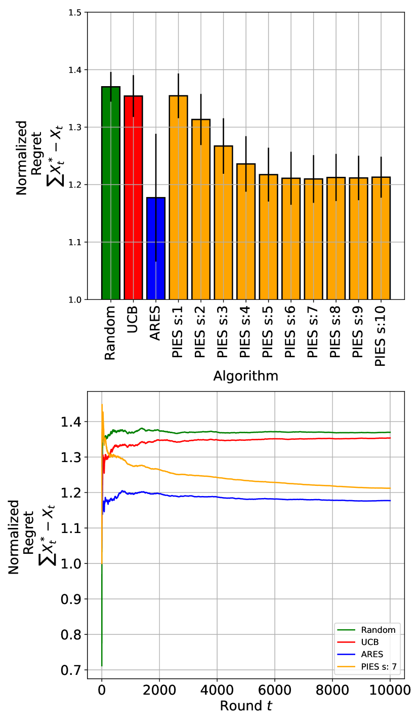
Figure 3: Ratio of average regret for each of the algorithms with respect to Oracle’s regret. Black lines are standard deviations.

Each simulation first iterates through $10,000$ rounds to set the system into the steady-state. The learner interacted with the system for $n=1,000$ rounds after the $10,000$ rounds. The proposed Algorithm 1 (ARES) is compared with an Oracle (where the chosen action $a\in[3]$ is the action $a$ that has the maximum $\hat{X}_{t}$ from the Kalman filter (3)), UCB [2], Random (for each round, the action is chosen uniformly random), and PIES [16]. PIES is preset with a parameter $s\in\{0,1,\dots,9,10\}$ which is the fixed window size of the algorithm. In Figure 3, the ratio between the algorithm’s regret with respect to the Oracle’s regret is computed and averaged across 100 simulations. For this particular randomly generated system, the regret for ARES is lower than PIES for any parameter $s\in\{0,1,\dots,9,10\}$ value and UCB. Figure 4 provides a rationale why this may be the case as the average chosen parameter $s$ value for action $a=1,3$ is $s=1$ and for action $a=2$ is $s=0$. This explains why the ARES algorithm has better performance than PIES as setting the same parameter $s$ for each action $a\in[k]$ may not be ideal for different environments.

The average $u_{a}$ value for each action $a=1,2,3$ is plotted in Figure 5. At the beginning, each action has a large $u_{a}$ value on average since the model $\hat{G}_{a}\left(\mathscr{T}_{a},s\right)$ error is large. Each of the $u_{a}$ values don’t converge to 0 due to the impact of the bias term $\beta_{a;t}$, but the magnitude of the reward $X_{t}$ is significantly larger than $u_{a}$ so the impact of the bias term $\beta_{a;t}$ is negligible. Finally, according to Figure 4, the average $s$ parameter chosen for action $a=2$ is smaller than the average $s$ parameter chosen actions $a=1,3$. Therefore, the $u_{a}$ value for action $a=2$ is smaller on average than the $u_{a}$ values of actions $a=1,3$ since the model size of action $a=2$ is smaller than action $a=1,3$ (i.e. less parameters to identify for action $a=2$ than actions $a=1,3$).

Remark 5.

The Oracle chooses actions based on the optimal prediction of the rewards from (1) in the mean-squared error sense as it assumes knowledge of (1). Therefore, the Oracle is not applicable for the considered setting. Rather, we use the Oracle as a baseline for regret performance.

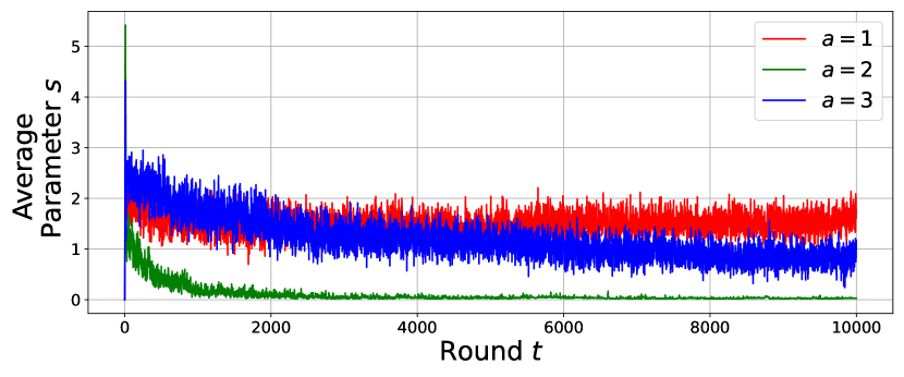
Figure 4: Each line on the plot indicates what parameter $s$ is chosen on average for each action $a\in\{1,2,3\}$. Here it can be observed that the average parameter $s$ values for action $a=3$ is different than $a=1,2$ $s$ values.

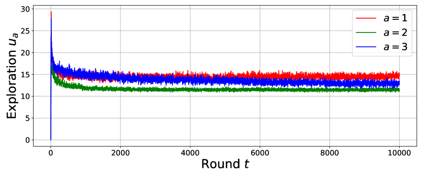
Figure 5: Each line on the plot is the average $u_{a}$ value for each action $a\in\{1,2,3\}$. The average $u_{a}$ for action $a=2$ is smaller than actions $a=1,3$ as the size of the model $s$ is smaller.

VIII Conclusion

This work has provided a perspective for extracting representations from non-stationary environments to predict rewards for each action. The results in this paper provided an algorithm that adaptively explores environments with rewards generated by linear dynamical systems. This is accomplished by utilizing an adaptive exploration method inspired by the UCB algorithm and also adjusting the size of the linear predictor for predicting rewards for each action. Future work will focus on the cases where the context $\theta_{t}$ may not be available at different time periods or just absent.

References

- [1] T. Lattimore and C. Szepesvári, Bandit algorithms. Cambridge University Press, 2020.
- [2] R. Agrawal, “Sample mean based index policies by o (log n) regret for the multi-armed bandit problem,” Advances in Applied Probability, vol. 27, no. 4, pp. 1054–1078, 1995.
- [3] A. Garivier and E. Moulines, “On upper-confidence bound policies for non-stationary bandit problems,” arXiv preprint arXiv:0805.3415, 2008.
- [4] C. Hartland, N. Baskiotis, S. Gelly, M. Sebag, and O. Teytaud, “Change point detection and meta-bandits for online learning in dynamic environments,” in CAp 2007: 9è Conférence francophone sur l’apprentissage automatique, 2007, pp. 237–250.
- [5] F. Liu, J. Lee, and N. Shroff, “A change-detection based framework for piecewise-stationary multi-armed bandit problem,” in Proceedings of the AAAI Conference on Artificial Intelligence, vol. 32, no. 1, 2018.
- [6] Y. Cao, Z. Wen, B. Kveton, and Y. Xie, “Nearly optimal adaptive procedure with change detection for piecewise-stationary bandit,” in The 22nd International Conference on Artificial Intelligence and Statistics. PMLR, 2019, pp. 418–427.
- [7] J. Mellor and J. Shapiro, “Thompson sampling in switching environments with bayesian online change detection,” in Artificial intelligence and statistics. PMLR, 2013, pp. 442–450.
- [8] N. Abe and P. M. Long, “Associative reinforcement learning using linear probabilistic concepts,” in ICML. Citeseer, 1999, pp. 3–11.
- [9] Y. Qin, T. Menara, S. Oymak, S. Ching, and F. Pasqualetti, “Representation learning for context-dependent decision-making,” in 2022 American Control Conference (ACC). IEEE, 2022, pp. 2130–2135.
- [10] Y. Qin, Y. Li, F. Pasqualetti, M. Fazel, and S. Oymak, “Stochastic contextual bandits with long horizon rewards,” arXiv preprint arXiv:2302.00814, 2023.
- [11] L. Wei and V. Srivastava, “Nonstationary stochastic multiarmed bandits: Ucb policies and minimax regret,” arXiv preprint arXiv:2101.08980, 2021.
- [12] O. Besbes, Y. Gur, and A. Zeevi, “Stochastic multi-armed-bandit problem with non-stationary rewards,” Advances in neural information processing systems, vol. 27, pp. 199–207, 2014.
- [13] L. Wei and V. Srivatsva, “On abruptly-changing and slowly-varying multiarmed bandit problems,” in 2018 Annual American Control Conference (ACC). IEEE, 2018, pp. 6291–6296.
- [14] P. Whittle, “Restless bandits: Activity allocation in a changing world,” Journal of applied probability, vol. 25, no. A, pp. 287–298, 1988.
- [15] A. Slivkins and E. Upfal, “Adapting to a changing environment: the brownian restless bandits.” in COLT, 2008, pp. 343–354.
- [16] J. Gornet, M. Hosseinzadeh, and B. Sinopoli, “Stochastic multi-armed bandits with non-stationary rewards generated by a linear dynamical system,” in 2022 IEEE 61st Conference on Decision and Control (CDC), 2022, pp. 1460–1465.
- [17] J. W. Mueller, V. Syrgkanis, and M. Taddy, “Low-rank bandit methods for high-dimensional dynamic pricing,” Advances in Neural Information Processing Systems, vol. 32, 2019.
- [18] S. Agrawal, S. Yin, and A. Zeevi, “Dynamic pricing and learning under the bass model,” in Proceedings of the 22nd ACM Conference on Economics and Computation, 2021, pp. 2–3.
- [19] P. Gradu, E. Hazan, and E. Minasyan, “Adaptive regret for control of time-varying dynamics,” in Proceedings of The 5th Annual Learning for Dynamics and Control Conference, ser. Proceedings of Machine Learning Research, N. Matni, M. Morari, and G. J. Pappas, Eds., vol. 211. PMLR, 15–16 Jun 2023, pp. 560–572. [Online]. Available: https://proceedings.mlr.press/v211/gradu23a.html
- [20] C. Tekin and M. Liu, “Online learning in opportunistic spectrum access: A restless bandit approach,” in 2011 Proceedings IEEE INFOCOM. IEEE, 2011, pp. 2462–2470.
- [21] L. Li, K. Jamieson, G. DeSalvo, A. Rostamizadeh, and A. Talwalkar, “Hyperband: A novel bandit-based approach to hyperparameter optimization,” The Journal of Machine Learning Research, vol. 18, no. 1, pp. 6765–6816, 2017.
- [22] M. Gagliolo and J. Schmidhuber, “Algorithm selection as a bandit problem with unbounded losses,” in International conference on learning and intelligent optimization. Springer, 2010, pp. 82–96.
- [23] J. Parker-Holder, V. Nguyen, and S. J. Roberts, “Provably efficient online hyperparameter optimization with population-based bandits,” Advances in neural information processing systems, vol. 33, pp. 17 200–17 211, 2020.
- [24] A. Tsiamis and G. J. Pappas, “Finite sample analysis of stochastic system identification,” in 2019 IEEE 58th Conference on Decision and Control (CDC). IEEE, 2019, pp. 3648–3654.
- [25] Y. Abbasi-yadkori, D. Pál, and C. Szepesvári, “Improved algorithms for linear stochastic bandits,” in Advances in Neural Information Processing Systems, J. Shawe-Taylor, R. Zemel, P. Bartlett, F. Pereira, and K. Q. Weinberger, Eds., vol. 24. Curran Associates, Inc., 2011.
- [26] S. Boucheron, G. Lugosi, and P. Massart, Concentration inequalities: A nonasymptotic theory of independence. Oxford university press, 2013.
- [27] R. Durrett, Probability: theory and examples. Cambridge university press, 2019, vol. 49.
- [28] A. H. Sayed, Adaptive Filters. Wiley-IEEE Press, 2008.