Suboptimality bounds for trace-bounded SDPs enable a faster and scalable low-rank SDP solver SDPLR+

Abstract

Semidefinite programs (SDPs) and their solvers are powerful tools with many applications in machine learning and data science. Designing scalable SDP solvers is challenging because by standard the positive semidefinite decision variable is an $n\times n$ dense matrix, even though the input is often an $n\times n$ sparse matrix. However, the information in the solution may not correspond to a full-rank dense matrix as shown by Bavinok and Pataki. Two decades ago, Burer and Monterio developed an SDP solver SDPLR that optimizes over a low-rank factorization instead of the full matrix. This greatly decreases the storage cost and works well for many problems. The original solver SDPLR tracks only the primal infeasibility of the solution, limiting the technique’s flexibility to produce moderate accuracy solutions. We use a suboptimality bound for trace-bounded SDP problems that enables us to track the progress better and perform early termination. We then develop SDPLR+, which starts the optimization with an extremely low-rank factorization and dynamically updates the rank based on the primal infeasibility and suboptimality. This further speeds up the computation and saves the storage cost. Numerical experiments on Max Cut, Minimum Bisection, Cut Norm, and Lovász Theta problems with many recent memory-efficient scalable SDP solvers demonstrate its scalability up to problems with million-by-million decision variables and it is often the fastest solver to a moderate accuracy of $10^{-2}$.

1 Introduction

Semidefinite programs (SDPs) are an extremely capable class of convex optimization problems. Conceptually, they generalize the class of vector decision variables used in linear programs to matrix decision variables. This creates optimization problems where the solution is a symmetric, positive semidefinite matrix. The class of semidefinite programs has many applications in machine learning including: matrix completion [18], k-means clustering [35, 65], combining SAT solvers and deep learning [64], along with many more applications in control theory [14]. In addition, SDPs have offered a systematic way of designing approximation algorithms for many NP-hard combinatorial problems, for instance, graph cut problems [27, 6, 30], graph clustering, and matrix cut-norm [3].

We consider SDPs of the following linear form

$$\mathop{\text{minimize}}_{\bm{X}\in\S^{n}}\;\langle\bm{C},\bm{X}\rangle\;\mathop{\text{subject to}}\;\calA(\bm{X})=\bm{\mathrm{b}},\bm{X}\succeq 0$$ (SDP)

where $\S^{n}$ is the set of symmetric matrices with size $n\times n$, $\bm{C}\in\S^{n}$ is a cost matrix, $\langle\cdot,\cdot\rangle$ denotes the inner product of two matrices $\langle\bm{A},\bm{B}\rangle=\smash{\sum_{ij}A_{ij}B_{ij}}$, and $\calA\mathrel{\mathop{\mathchar 58\relax}}\S^{n}\to\R^{m}$ is a linear operator encoding $m$ linear constraints with right-hand side vector $\bm{\mathrm{b}}$. The constraint notation $\mathcal{A}(\bm{X})$ corresponds to the vector $[\langle\bm{A}_{1},\bm{X}\rangle,\ldots,\langle\bm{A}_{m},\bm{X}\rangle]^{T}$. As a convex problem, (SDP) can be solved to high accuracy via interior point methods on small problem instances [11, 59, 61]. Interior point methods, however, cannot solve large problem instances due to the memory needed to store the decision variable with $n^{2}$ entries and the second-order information. This property has made scaling SDPs to large problem instances, where $n$ is in the millions, challenging and, consequently, has focused a long and continuing thread of research on scaling SDPs.

Among scalable SDP solvers, possibly the most famous one is the Burer and Monterio solver SDPLR [16, 17, 15]. It was developed based on the observation that (SDP) admits an optimal solution with rank $O(\sqrt{m})$ based on a bound by Bavinok and Pataki [9, 49]. Therefore, they factorize the decision variable $\bm{X}$ into $\bm{Y}\bm{Y}^{T}$ with $\bm{Y}$ having size $n\times r$ where $r=\Theta(\sqrt{m})$ and transform (SDP) into the following (BM-SDP).

$$\mathop{\text{minimize}}_{\bm{Y}\in\R^{n\times r}}\;\langle\bm{C},\bm{Y}\bm{Y}^{T}\rangle\;\mathop{\text{subject to}}\;\calA(\bm{Y}\bm{Y}^{T})=\bm{\mathrm{b}}$$ (BM-SDP)

This transformation naturally eliminates the hard-to-optimize positive semidefiniteness constraint and SDPLR tackles (BM-SDP) using the augmented Lagrangian (ALM) framework. The drawback of this transformation is that it leads to a nonconvex problem and the convergence to the global optimum is not guaranteed. Recent research [12, 19] has shown that for a generic problem instance, any local optimum of (BM-SDP) is a global optimum when $r=\Omega(\sqrt{m})$, and non-generic exceptions are possible [47].

Also recently, another line of research studies memory-efficient SDP solvers based on the Frank-Wolfe method [31]. Regardless of how the Frank-Wolfe method is integrated into the SDP solvers, it typically requires an easy-to-characterize compact domain for solving the linear optimization subproblems efficiently [29, 69, 55, 56, 50, 68]. Often this is a class of trace-bounded SDPs

$$\mathop{\text{minimize}}_{\bm{X}\in\Delta_{\alpha}}\;\langle\bm{C},\bm{X}\rangle\;\mathop{\text{subject to}}\;\mathcal{A}(\bm{X})=\bm{\mathrm{b}}$$ (Trace-Bounded SDP)

where $\Delta_{\alpha}=\left\{\bm{X}\succeq 0\mathrel{\mathop{\mathchar 58\relax}}\text{Tr}(\bm{X})\leqslant\alpha\right\}$ is the convex cone of positive semidefinite matrices with trace bounded by a constant $\alpha\geqslant 0$. For this set, the linear optimization subproblem involved in Frank-Wolfe turns into an eigenvalue problem. One can see (Trace-Bounded SDP) has the same optimum with (SDP) if we pick $\alpha\geqslant\text{Tr}(\bm{X}^{*})$ where $\bm{X}^{*}$ is an optimal solution. While (Trace-Bounded SDP) is only a subclass of (SDP), many SDPs used in applications directly have a trace bound encoded by the constraints, or have a trace bound that can be estimated. Examples include $k$-means [35, 65], graph cuts [30, 24], phase retrieval [7], correlation clustering [8], and those we test in the experiments.

One advantage of these Frank-Wolfe methods over SDPLR is they have an easy-to-compute surrogate duality bound for tracking the suboptimality. This enables them to track the progress more precisely and terminate the optimization efficiently. Numerical experiments demonstrate their scalability on large-scale problems, especially for moderately accurate solutions [50, 69]. We note that SDPLR does not track the suboptimality because the dual problem of (SDP) has a feasible region with a tricky constraint that requires a particular matrix to be positive semidefinite.

Our core contribution in this paper is that we design a faster and more scalable SDP solver called SDPLR+ based on combining SDPLR with two techniques.

• We use the fact that the trace bound in (Trace-Bounded SDP) results in an unconstrained dual problem where strong duality always holds (Theorem 1). This enables any solver with both primal and dual estimates to have a suboptimality bound, including SDPLR (Section 3.1).

• The suboptimality bound and primal infeasibility bound allow us to design a solver tolerant of smaller rank iterates. Since we can track progress better, we start the optimization from an extremely small rank parameter $r$ and dynamically update the rank when no progress is made after a while. This speeds up the computation and reduces the memory cost.

• The code is available at https://github.com/luotuoqingshan/SDPLRPlus.jl.

We demonstrate the new solver through comprehensive experiments using over 200 instances of Maximum Cut, Minimum Bisection, Lovász Theta, and Cut Norm SDPs. These experiments show that this simple combination is often faster and more scalable than recently proposed Frank-Wolfe based methods for computing moderately accurate solutions.

2 Preliminaries

Matrices and vectors are written in bold. The norm $\|\cdot\|$ refers to the 2-norm of a vector and the spectral norm of a matrix, and $\|\cdot\|_{F}$ denotes the Frobenius norm of a matrix.

Let $G=(V,E)$ denote an undirected graph with vertex set $V$ and edge set $E$. We let $uv$ denote the undirected edge between vertex $u$ and $v$. Each edge $uv\in E$ is assigned a weight $w(uv)$. Non edges have weight 0. For any vertex set $S$, let $\bar{S}=V\setminus S$ be its complement and the value of the cut induced by $S$ is $\textbf{cut}(S,\bar{S})=\sum_{u\in S,v\in\bar{S}}w(uv)$. Let $\bm{L}$ be the Laplacian matrix of an undirected graph where $\bm{L}_{i,j}=-w(ij)$ if $i\neq j$ and $\bm{L}_{i,i}=\smash{\sum_{j}w(ij)}$.

3 Methodology and Algorithm

In this section, we describe how we design SDPLR+ to provide more quality guarantees and make it more scalable than SDPLR for (Trace-Bounded SDP). We begin with a theoretical result about SDPs.

3.1 Strong duality and a suboptimality bound

We design a suboptimality bound by using the fact that the trace bound in (Trace-Bounded SDP) results in an unconstrained dual problem where strong duality always holds. In optimization, a suboptimality bound tells us how far the current objective is away from the optimum, which gives a precise measure of progress for the solver. In the context of (SDP), a suboptimality bound is any valid upper bound of $\langle\bm{C},\bm{X}\rangle-\langle\bm{C},\bm{X}^{*}\rangle$ where $\bm{X}^{*}$ is the optimum of (SDP).

A key tool for deriving a suboptimality bound is duality. Consider the dual problem for (SDP)

$$\mathop{\smash{\text{sup}}}_{\bm{\mathrm{\lambda}}}\;\bm{\mathrm{\lambda}}^{T}\bm{\mathrm{b}}\;\mathop{\text{subject to}}\;\bm{C}-\calA^{*}(\bm{\mathrm{\lambda}})\succeq 0,$$ (SDD)

where $\calA^{*}\mathrel{\mathop{\mathchar 58\relax}}\R^{m}\to\S^{n}$ is the adjoint of $\calA$. By duality of convex programs, any feasible solution to (SDD) has a dual value at most $\langle\bm{C},\bm{X}^{*}\rangle$. Therefore the gap between $\langle\bm{C},\bm{X}\rangle$ and the dual value serves as a suboptimality bound. However, finding a non-trivial feasible solution to (SDD) is not easy because of the positive semidefinite constraint $\bm{C}-\calA^{*}(\bm{\mathrm{\lambda}})\succeq 0$. Also, unless the SDP satisfies strong duality, there may exist a gap between the primal and dual solutions – see an example in Appendix A.

The trace bound in (Trace-Bounded SDP), however, changes the picture entirely. Consider the dual of (Trace-Bounded SDP)

$$\mathop{\smash{\text{sup}}}_{\bm{\mathrm{\lambda}}}\;\bm{\mathrm{\lambda}}^{T}\bm{\mathrm{b}}+\alpha\mathop{\text{min}}\{\lambda_{\mathop{\text{min}}}(\bm{C}-\calA^{*}(\bm{\mathrm{\lambda}})),0\},$$ (Trace-bounded SDD)

we have the following result which characterizes the relation between (Trace-Bounded SDP) and (Trace-bounded SDD).

Theorem 1.

Strong duality always holds between (Trace-Bounded SDP) and (Trace-bounded SDD), and the optimum of (Trace-Bounded SDP) can be attained.

Proof.

Note that the space of $n\times n$ real matrices can be viewed as $\R^{n^{2}}$. We first show that $\Delta_{\alpha}$ is a compact set lying in this space. To show the compactness of $\Delta_{\alpha}$, we use Heine–Borel theorem to turn it into proving $\Delta_{\alpha}$ is closed and bounded. The set $\Delta_{\alpha}$ is closed as it is the intersection of two closed sets: (a) the semidefinite cone $\{\bm{X}\in\S^{n}\mathrel{\mathop{\mathchar 58\relax}}\bm{X}\succeq 0\}$ and (b) the set of trace-bounded matrices. The set $\Delta_{\alpha}$ is bounded because

$$\|\bm{X}\|_{F}=\sqrt{\text{Tr}(\bm{X}\bm{X}^{T})}=\sqrt{\text{Tr}(\bm{X}^{2})}\leqslant\sqrt{\lambda_{\mathop{\text{max}}}(\bm{A})\text{Tr}(\bm{X})}\leqslant\sqrt{\text{Tr}(\bm{X})^{2}}\leqslant\alpha$$

where we used a known inequality $\text{Tr}(\bm{A}\bm{B})\leqslant\lambda_{\mathop{\text{max}}}(\bm{A})\text{Tr}(\bm{B})$ for positive semidefinite matrices (instances of this date back to at least [32]).

Now let $f(\bm{X},\bm{\mathrm{\lambda}})=\langle\bm{C},\bm{X}\rangle-\bm{\mathrm{\lambda}}^{T}(\mathcal{A}(\bm{X})-\bm{\mathrm{b}})$. Because $\Delta_{\alpha}$ is compact and convex, and both $f(\cdot,\bm{\mathrm{\lambda}})$ and $f(\bm{X},\cdot)$ are linear, Sion’s minimax theorem [58] says

$$\eqref{eq:3}=\mathop{\text{min}}_{\bm{X}\in\Delta_{\alpha}}\mathop{\smash{\text{sup}}}_{\bm{\mathrm{\lambda}}}f(\bm{X},\bm{\mathrm{\lambda}})=\mathop{\smash{\text{sup}}}_{\bm{\mathrm{\lambda}}}\mathop{\text{min}}_{\bm{X}\in\Delta_{\alpha}}f(\bm{X},\bm{\mathrm{\lambda}})=\eqref{eq:12}.$$

The optimum of (Trace-Bounded SDP) can be attained because $\Delta_{\alpha}$ is compact. ∎

We suspect Theorem 1 may be known, although we cannot find a reference to it despite extensive searching. To help understand why this result changes the picture of duality – and closes the duality gap for SDPs – we present a study with a common example of a duality gap in Appendix A.

Corollary 2.

Because (Trace-bounded SDD) is unconstrained, any $\bm{\mathrm{\lambda}}$ is feasible for this dual problem. As a result any dual solution lower bounds $\langle\bm{C},\bm{X}^{*}\rangle$ and gives the following suboptimality bound

$$\langle\bm{C},\bm{X}\rangle-\langle\bm{C},\bm{X}^{*}\rangle\leqslant\langle\bm{C},\bm{X}\rangle-\bm{\mathrm{\lambda}}^{T}\bm{\mathrm{b}}-\alpha\mathop{\text{min}}\{\lambda_{\mathop{\text{min}}}(\bm{C}-\calA^{*}(\bm{\mathrm{\lambda}})),0\}.$$ (1)

The bound in this corollary is also present in [22, 5], although that bound is presented under the assumption that strong duality holds. Our results show this is not necessary.

Although this may look simple, it turns out better and cleaner than existing suboptimality bounds. Boumal et al. [12] give one suboptimality bound from the Riemannian optimization perspective, which however requires a strong assumption that the gradient of all constraints $\calA(\bm{Y}\bm{Y}^{T})$ are independent for all $\bm{Y}$ on the manifold $\calM=\{\bm{Y}\in\R^{n\times r}\mathrel{\mathop{\mathchar 58\relax}}\calA(\bm{Y}\bm{Y}^{T})=\bm{\mathrm{b}}\}$. Yurtsever et al. [69] also address (Trace-Bounded SDP) but gives one suboptimality bound by considering the Frank-Wolfe surrogate duality gap for the augmented Lagrangian. Their suboptimality bound has a more complicated form and by simple algebraic manipulation, one can discover it has some inherent connection with (1) but worse, which we illustrate in Appendix B.

3.2 Implicit links to the trace-bounded dual in SDPLR

The goal of this section is to explain that the augmented Lagrangian strategy in SDPLR should do a reasonable job of producing primal and dual iterates that are tight in terms of the suboptimality bound (1). To do so, we need a brief recap of the augmented Lagrangian method, before describing how the subproblems map into our setting.

The augmented Lagrangian method is a popular framework for constrained optimization problems (see [46] for example). Consider constrained problems of the following form

$$\mathop{\text{minimize}}_{\bm{\mathrm{x}}\in\calD}\;f(\bm{\mathrm{x}})\;\mathop{\text{subject to}}\;g(\bm{\mathrm{x}})=$$

where $f\mathrel{\mathop{\mathchar 58\relax}}\calD\to\R$ is a real-valued objective function and $g\mathrel{\mathop{\mathchar 58\relax}}\calD\to\R^{m}$ encodes $m$ constraints. From a minimax perspective, (3.2) can be equivalently formulated as $\mathop{\text{min}}_{\bm{\mathrm{x}}\in\calD}\mathop{\text{max}}_{\bm{\mathrm{\lambda}}}f(\bm{\mathrm{x}})-\bm{\mathrm{\lambda}}^{T}g(\bm{\mathrm{x}})$ where $\bm{\mathrm{\lambda}}$ is the Lagrangian multipliers. However, the inner $\mathop{\text{max}}_{\bm{\mathrm{\lambda}}}$ can be nonsmooth. The ALM framework tackles this by introducing a quadratic proximal term penalizing $\bm{\mathrm{\lambda}}$ deviating from the prior estimate $\bar{\bm{\mathrm{\lambda}}}$, which in turn gives the following minimax problem

$$\mathop{\text{min}}_{\bm{\mathrm{x}}\in\calD}\mathop{\text{max}}_{\bm{\mathrm{\lambda}}}f(\bm{\mathrm{x}})-\bm{\mathrm{\lambda}}^{T}g(\bm{\mathrm{x}})-\frac{1}{2\sigma}\|\bm{\mathrm{\lambda}}-\bar{\bm{\mathrm{\lambda}}}\|^{2}.$$ (2)

We can see that the inner maximum of (2) is attained at

$$\bm{\mathrm{\lambda}}=\bar{\bm{\mathrm{\lambda}}}-\sigma g(\bm{\mathrm{x}})$$ (3)

and plug it into (2) simplifies the outer minimization problem to

$$\mathop{\text{min}}_{\bm{\mathrm{x}}\in\calD}f(\bm{\mathrm{x}})-\bar{\bm{\mathrm{\lambda}}}^{T}g(\bm{\mathrm{x}})+\frac{\sigma}{2}\|g(\bm{\mathrm{x}})\|^{2}.$$ (4)

A standard ALM implementation involves solving the inner and outer optimization problems of (2) alternatively and (3), (4) are usually referred to as dual and primal updates. Usually $\sigma$ will increase across iterations to sharpen the proximal term, which is quite intuitive as (2) is equivalent to (3.2) when $\sigma\rightarrow\infty$.

We use the ALM method to provide good primal and dual estimates for (Trace-Bounded SDP) and (Trace-bounded SDD) in SDPLR+, as it was used in SDPLR. In particular, the primal update is

$$\mathop{\text{minimize}}_{\bm{X}\in\Delta_{\alpha}}\;\langle\bm{C},\bm{X}\rangle-\bar{\bm{\mathrm{\lambda}}}^{T}\left(\mathcal{A}(\bm{X})-\bm{\mathrm{b}}\right)+\frac{\sigma}{2}\|\mathcal{A}(\bm{X})-\bm{\mathrm{b}}\|^{2},$$

and the dual update is $\bm{\mathrm{\lambda}}=\bar{\bm{\mathrm{\lambda}}}-\sigma(\mathcal{A}(\bm{X})-\bm{\mathrm{b}})$. Using the Burer-Monterio factorization over the factors $\bm{Y}\bm{Y}^{T}$ of $\bm{X}$ turns the primal and dual updates into

$$\mathop{\text{minimize}}_{\bm{Y}\in\R^{n\times r}\mathrel{\mathop{\mathchar 58\relax}}\text{Tr}(\bm{Y}\bm{Y}^{T})\leqslant\alpha}\;\langle\bm{C},\bm{Y}\bm{Y}^{T}\rangle-\bar{\bm{\mathrm{\lambda}}}^{T}\left(\mathcal{A}(\bm{Y}\bm{Y}^{T})-\bm{\mathrm{b}}\right)+\frac{\sigma}{2}\|\mathcal{A}(\bm{Y}\bm{Y}^{T})-\bm{\mathrm{b}}\|^{2}$$

and $\bm{\mathrm{\lambda}}=\bar{\bm{\mathrm{\lambda}}}-\sigma(\mathcal{A}(\bm{Y}\bm{Y}^{T})-\bm{\mathrm{b}})$. There is a strong parallelism between these updates and the primal, dual updates of SDPLR. The only difference is the constraint $\text{Tr}(\bm{Y}\bm{Y}^{T})\leqslant\alpha$, which is usually not violated badly because the trace bound encoded in the constraints implicitly prevent it from deviating too much. Intuitively, this shows that although originally designed to provide estimates for (SDP) and (SDD), SDPLR is implicitly optimizing the primal and dual of the trace-bounded version. This shows why this particular bound is likely to be successful.

3.3 The overall SDLPR+ algorithm and dynamic rank updates

In the interest of space, we state the full SDPLR+ algorithm in Appendix C. We briefly summarize key points of the overall approach here. Like SDPLR, we use the augmented Lagrangian approach overall. The minimization problem in the primal update is approximately solved using L-BFGS [41]. The line search in L-BFGS is performed by solving a cubic equation [15].

Eigenvalue Computation

One critical computation involved in evaluating the suboptimality bound is evaluating the minimum eigenvalue of $\bm{C}-\calA^{*}\bm{\mathrm{\lambda}}$. We use the Lanczos method with random start [34] and adopt the memory-efficient implementation from [69]. In our case, we mainly compute the minimum eigenvalue when evaluating the suboptimality to determine if to terminate, hence we run the Lanczos method for more steps to gain a higher accuracy. In particular, we take $2\sqrt{t}\log n$ steps, where $t$ is the number of L-BFGS iterations we have performed.

Dynamic Rank Update

Although Burer-Monterio based methods have good theoretical guarantees when $r=\Omega(\sqrt{m})$, a decision variable $\bm{Y}$ with $\Omega(n\sqrt{m})$ non-zero entries is still far from scalable. Hence in practice, a much smaller rank is usually picked to speed up the computation and save the storage cost. The downside is that Burer-Monterio based methods may fail to converge to the optimum. A common strategy is to increase the rank dynamically. SDPLR and Manopt+ [16, 12] both dynamically increase the rank from a small number to $\Omega(\sqrt{m})$, but they either do not consider early termination or implement early termination based on the heuristic that the answer is close to the optimum if the change of objective value is small across two consecutive iterations. Now because we have an easy-to-compute suboptimality bound, we can terminate the dynamic rank update once the desired suboptimality precision is achieved.

4 Related Work

For detailed discussions on solving Semidefinite programs, see the surveys [43, 66], and for discussion of low-rank solutions, see [36]. This section discusses the most relevant related work.

4.1 Scalable SDP solvers

The two most related classes of scalable SDP solvers are Burer-Monterio based methods and Frank-Wolfe based methods. As mentioned before, the core idea of Burer-Monterio based methods is to optimize over the low-rank factors of the decision matrix. Besides SDPLR, another line of Burer-Monterio methods is Riemannian optimization based, which optimizes the low-rank factors on the Riemannian manifolds with or without extra constraints, instead of in the Euclidean space [12, 40]. Concurrently to our research, Monterio et al. [44] proposed an efficient augmented Lagrangian method for (Trace-Bounded SDP) based on combining an adaptive inexact proximal point method with inner acceleration and Frank-Wolfe steps.

Roughly the Frank-Wolfe based methods can be categorized into two classes: (1) Yurtsever et al. propose a solver CGAL [68] that tackles the constrained problem (SDP) via the augmented Lagrangian method where the primal update is performed by one Frank-Wolfe update instead of the conventional minimization. Furthermore, they propose a more scalable solver which uses efficient sketching techniques for symmetric positive semidefinite matrices to cut the memory usage [62, 69]. (2) Another line is similar to the penalty method that integrates the constraints into the objective with properly chosen penalty function and coefficient, and optimizes the objective efficiently using Frank-Wolfe method [29]. In this vein, Shinde et al. [55, 56] recently observed that for SDPs that are designed for combinatorial problems and have a hyperplane rounding algorithm, one can cut the memory cost by only tracking one random vector with a distribution $\mathcal{N}(\bm{\mathrm{0}},\bm{X})$. In this way, $\bm{X}$ is implicitly encoded and is not required to be stored. Recently, Pham et al. [50] combined this extreme point sampling idea with a reformulation from Nesterov [45] to design a scalable SDP solver SCAMS for Max Cut.

Concurrent to our work, Angell and McCallum designed USBS which adapts spectral bundle and combines it with sketching [5]. This demonstrates a scalable solver in tests with $n$ in the millions.

4.2 Theoretical Guarantees of Burer-Monterio Methods

Due to the great empirical success of Burer-Monteiro method, there has been an extensive effort for developing theory for it. Recently Boumal et al. [12, 13] showed that by assuming the feasible set is a smooth manifold, cost matrix $\bm{C}$ is generic and $r$ satisfied $r(r+1)/2>m$, then equality-constrained SDPs have no spurious 2nd-order critical points. Put another way, all 2nd-order critical points are global optimums under the forementioned conditions. Cifuentes [19] generalized their result to broader classes of SDPs. On the other hand, Waldspurger and Waters [63] show that the Barvinok-Pataki bound is essential as the 2nd-order critical points of Burer-Monteiro are not generically optimal even if the SDP admits a global optimal solution with rank lower than Barvinok-Pataki bound. O’Carroll et al. [47] show that the assumption that the cost matrix is generic is necessary and construct examples where Burer-Monteiro has spurious 2nd-order critical points. Finally, in the setting of smooth analysis, Cifuentes and Moitra [20] show that for $r$ larger than the Barvinok-Pataki bound, the Burer-Monteiro method can provide an SDP solution to any accuracy in polynomial time.

5 Experiments

We evaluate our algorithm and a variety of other solvers on over 200 problems in a test set we describe in the following section. While we would have hoped to test all of the recently proposed solvers, we were unable to find code available for [44] and found the code for [5] too late to include in the results (the code was not linked in the paper, we do some limited comparison in Appendix E to show that we are likely faster in many scenarios). Since the remaining solvers are written in many different programming languages, we evaluate all solvers in a single threaded scenario with many single threaded solvers running concurrently. This should be the most energy efficient and representative scenario given the dynamic frequency scaling of modern CPUs. We ran our evaluation on different servers with slightly different processors. In order to compare across problems, we guarantee that all solvers on a given problem instance were run on the same server. We also limit total RAM access for each solver to 16GB and limit each solver to a runtime of 8 hours. On all problem instances, we start the dynamic rank update of SDPLR+ from 10, and set the L-BFGS history size to 4. More details are included in Appendix D.

Through all the evaluations, we stop all the optimizers according to the following quality metrics: $\displaystyle\frac{\|\mathcal{A}(\bm{X})-\bm{\mathrm{b}}\|}{1+\|\bm{\mathrm{b}}\|}$ (Primal Infeasibility) $\displaystyle\frac{\langle\bm{C},\bm{X}\rangle-\langle\bm{C},\bm{X}^{*}\rangle}{1+|\langle\bm{C},\bm{X}\rangle|}$ (Suboptimality)

We study the solvers on four distinct problems: Max Cut, Minimum Bisection, Lovász Theta, and Cut Norm. We only evaluated a solver if the authors provided an implementation for solving SDP or if it could be implemented in a way where we were confident would accurately represent performance.

5.1 Datasets

The SDPs we use correspond to graph problems. As such, there is a wealth of possible data for benchmarking the solvers. We chose these graphs based on other comparisons of SDP solvers.

• Gset [21]: This is a set of 71 randomly generated square matrices with either binary or $-1,0,+1$ values. Sizes range from 800 to 20000 rows and up to 80000 non-zero entries.

• SNAP Datasets [37]: We pick a list of 4 web graphs and 11 community graphs from SNAP, including ca-AstroPh [38], web-BerkStan [39], and com-youtube [67].

• DIMACS10 [21]: This is a set of 151 different kinds of graphs from the 10th DIMACS Implementation Challenge for graph partitioning and graph clustering subtasks. We pick a subset of 116 graphs with the largest ones having $n=\text{1,048,576}$ and 89,239,674 nonzeros.

In total we build a collection of 202 graphs. More information and statistics of datasets we use are included in Appendix D.1. For all the graphs, we drop directions and symmetrize the adjacency matrix if they are directed. For SNAP datasets, we take the largest components of the graphs and remove self-loops.

5.2 Performance Profile Plots

We use performance profile plots [23, 48] to compare the solvers across this range of problems. Since each solver may not be the fastest or best on every problem instance, this shows a profile of how often the solvers are within a $\tau$-bound of the best. It’s reminiscent of a receiver-operator curve or precision-recall curve. The goal is to be “up and to the left” in this case. This means that a given solver was the best or within a small factor of being the best on the largest number of problems. For all performance profile plots throughout this paper, the x-axis $\tau$ represents the ratio between the current solver and the best one with regard to a specific metric (time or discrete objective value). The point on the right of a solver curve corresponds to what fraction of the total set of problems it solved within the time bound.

5.3 Max Cut

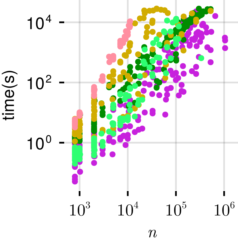
(a) Runtime by Problem Size

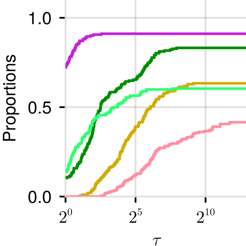
(b) Perf. Prof. of Runtime

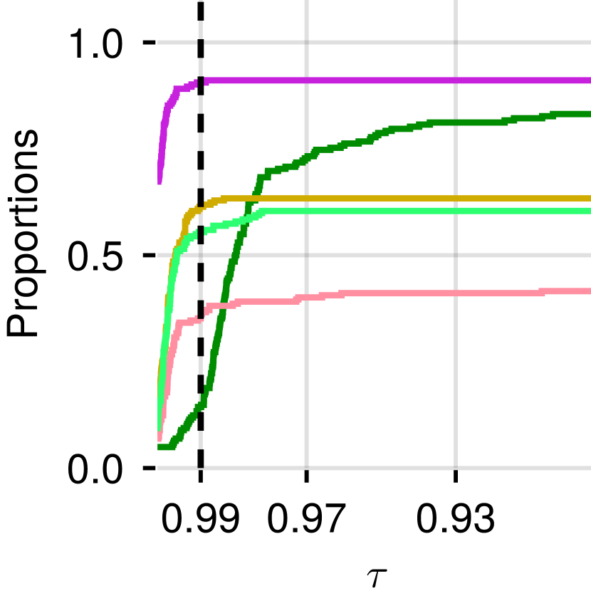
(c) Perf. Prof. of Rounded Cuts

Figure 1: Results on Max Cut. We set tolerance $\varepsilon=10^{-2}$, and test each solver on all 202 graphs. We time out each solver after 8 hours. Figure 1(a) and 1(b) display how the running time of each solver scales with the problem size $n$ and the running time performance profile plot of all the solvers respectively. Note that SDPLR+ is the fastest solver for most of the problem instances and is within a small factor of the optimal solver for the other instances. While SCAMS also exhibits good scalability, from Figure 1(c), we see that it usually produces smaller cuts.

Max Cut is a combinatorial problem which aims at finding the maximum cut induced by any vertex set $S$, i.e. solving $\mathop{\text{max}}_{S\subseteq V}\textbf{cut}(S,\bar{S})$. Because Max Cut is NP-hard to solve, a common strategy is relaxing it to the following semidefinite program and then rounding the real solution to a discrete partition $(S,\bar{S})$ [27],

$$\mathop{\text{maximize}}_{\bm{X}\succeq 0}\;\tfrac{1}{4}\langle\bm{L},\bm{X}\rangle\;\mathop{\text{subject to}}\;\mathop{\text{diag}}(\bm{X})=\bm{\mathrm{1}}.$$ (Max Cut)

On Max Cut, we compare our method against the following solvers:

1. CSDP [11]: A C library for solving (SDP) using predictor and corrector algorithm. CSDP provides both primal and dual solutions.

2. SketchyCGAL [69]: A low-rank variant of CGAL method which sketches the primal variable of CGAL using Nystrom Sketching, which has great scalability for producing moderately accurate solutions. We set the sketching size $R=10$ throughout all experiments.

3. SCAMS [50]: A memory-efficient Frank-Wolfe based solver designed specifically for (Max Cut).

4. Riemannian Optimization Methods: We adopt one efficient Riemannian optimization implementations designed for (Max Cut) in [12], Manopt. They turn the diagonal-constrained (Max Cut) into an unconstrained optimization problem on the Oblique manifold $\text{OB}(r,n)=\{\bm{Y}\in\R^{n\times r}\mathrel{\mathop{\mathchar 58\relax}}\mathop{\text{diag}}(\bm{Y}\bm{Y}^{T})=\bm{\mathrm{1}}\}$ and apply Riemannian Trust Region method [1]. Manopt sets $r=\lceil\frac{\sqrt{8n+1}}{2}\rceil$ which satisfies the Barvinok-Pataki bound.

Because SCAMS requires positive degrees, we preprocess all graphs to take the absolute value of edge weights to make sure all edge weights are positive for Max Cut.

For a given tolerance parameter $\varepsilon$, we stop SDPLR+, SketchyCGAL and Manopt when their (Primal Infeasibility) and (Suboptimality) are both smaller than $\varepsilon$. Manopt originally terminates based on the norm of the Riemannian gradient, we exploited the suboptimality bound for Max Cut introduced in [12] to let it stop based on the suboptimality. In particular, we exponentially decay the Riemannian gradient norm tolerance from an initial value of 10 by a factor of 5 until the suboptimality reaches the desired accuracy $\varepsilon$. Because SCAMS is solving a reformulation whose optimum is the square root of the optimum of (Max Cut), we set its tolerance as $\frac{\varepsilon}{2}$. Besides (Primal Infeasibility), CSDP has two more metrics, dual infeasibility and relative duality gap (we introduce them more in Appendix D.3), we set their tolerance all to $\varepsilon$. We pick the trace bound $\alpha$ as $n$ for SDPLR+ and SketchyCGAL. Furthermore, as Max Cut has a nice hyperplane rounding algorithm to extract discrete solutions from the SDP solutions, we compare the quality of the rounded cuts induced by SDP solutions of different solvers. The results are summarized in Figure 1. Overall, SDLPR+ shows better scalability and solution quality.

5.4 Minimum Bisection

Minimum Bisection [26] tries to find a good bisection which minimizes the bisection width, which has numerous applications [57, 54]. Formally, it aims at dividing the vertex set $V$ into two sets $S,\bar{S}$ with equal size, i.e. $|S|=|\bar{S}|$ and minimizing $\textbf{cut}(S,\bar{S})$. The corresponding SDP relaxation is

$$\mathop{\text{minimize}}_{\bm{X}\succeq 0}\;\tfrac{1}{4}\langle\bm{L},\bm{X}\rangle\;\mathop{\text{subject to}}\;\mathop{\text{diag}}(\bm{X})=\bm{\mathrm{1}},\bm{\mathrm{1}}^{T}\bm{X}\bm{\mathrm{1}}=0.$$ (Minimum Bisection)

Because the original minimum bisection aims to divide the graph into two equal-size pieces, we add one dummy isolated vertex if needed. In addition to comparing the generic SDP solvers SketchyCGAL and CSDP, we compare with three simple constrained Riemannian optimization solvers implemented in [40], which are Riemannian Augment Lagrangian method (RALM), exact penalty method with smoothing via the log-sum-exp function ($\text{Q}^{\text{lse}}$) and via a pseudo-Huber loss and a linear-quadratic loss ($\text{Q}^{\text{lqh}}$). Because RALM, $\text{Q}^{\text{lse}}$, $\text{Q}^{\text{lqh}}$ have quite complicated terminating conditions, we keep them unchanged. We pick the trace bound $\alpha$ as $n$ for SDPLR+ and SketchyCGAL. We also apply hyperplane rounding to extract bisections from SDP solutions. We regard solutions provided by RALM, $\text{Q}^{\text{lse}}$, $\text{Q}^{\text{lqh}}$ with objective $\frac{1}{4}\langle\bm{L},\bm{X}\rangle$ larger than $(1+\varepsilon)$ times the size of the best minimum bisection extracted underoptimized and discard them. The results are summarized in Figure 2. Again, we see a clear advantage to SDPLR+ in speed and accuracy.

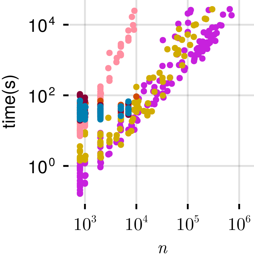
(a) Runtime by Problem Size

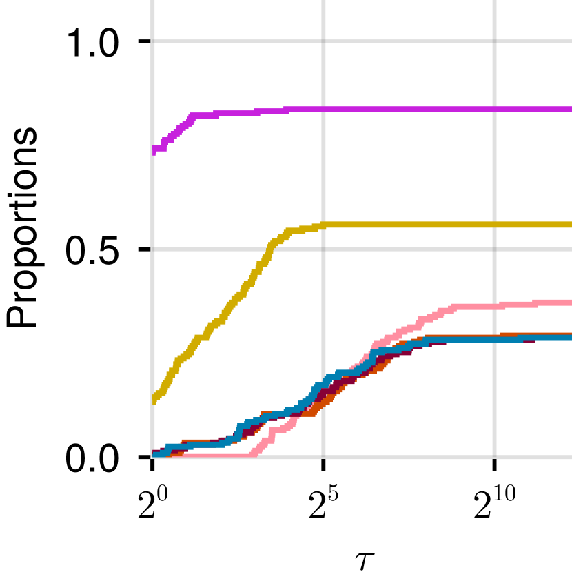
(b) Perf. Prof. of Runtime

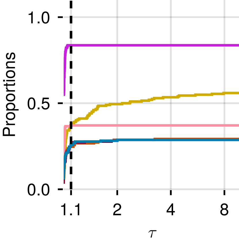
(c) Perf. Prof. of Rounded Cuts

Figure 2: Results on Minimum Bisection. We set tolerance $\varepsilon=10^{-2}$, and test each solver on all 202 graphs. We time out each solver after 8 hours. Figure 2(a) and 2(b) display how the running time of each solver scales with the problem size $n$ and the running time performance profile plot of all the solvers respectively. Note that SDPLR+ is overall the fastest solver. The constrained Riemannian optimization methods fail on over half of the problems. From Figure 2(c), we see SDPLR+ often provides a better rounded minimum bisection than SketchyCGAL.

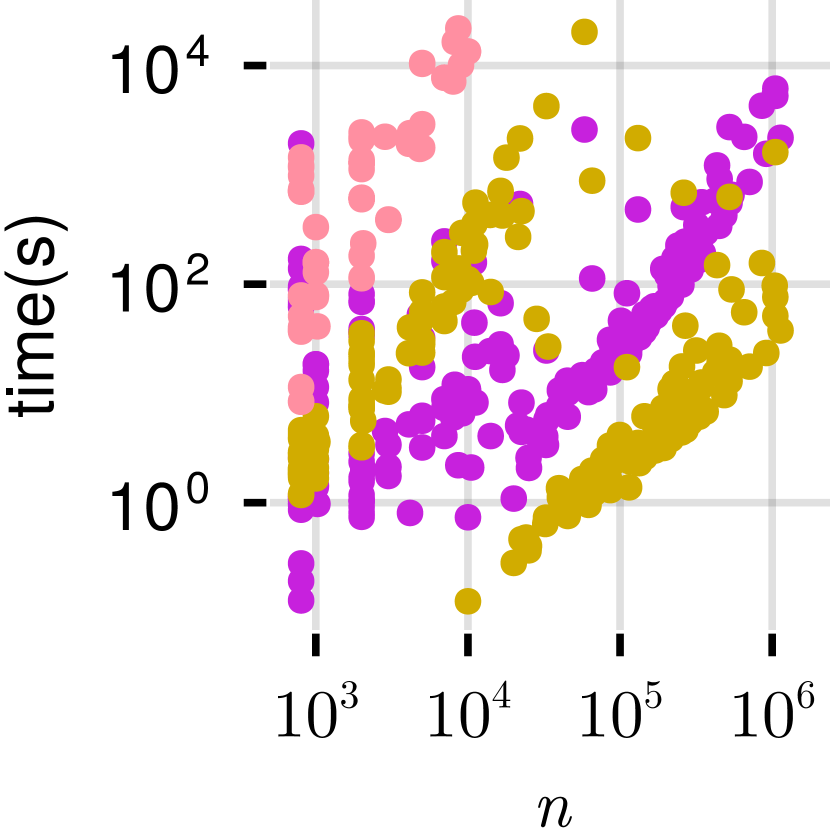
(a) Lovàsz Theta Runtime by Prob. Size

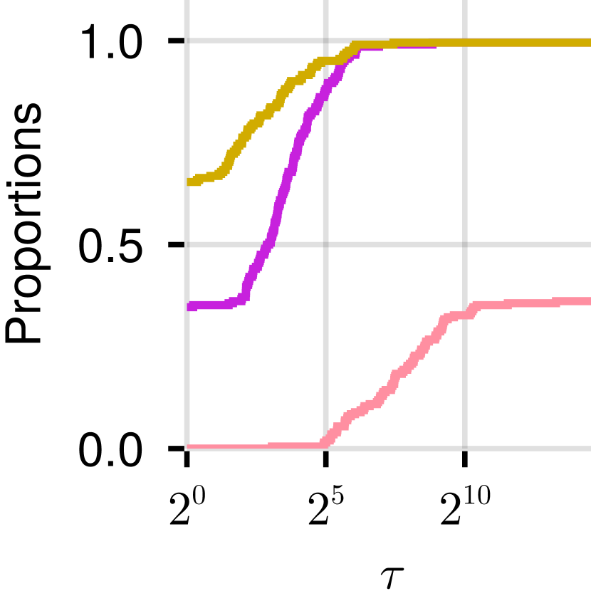
(b) Lovàsz Theta Runtime Perf. Prof.

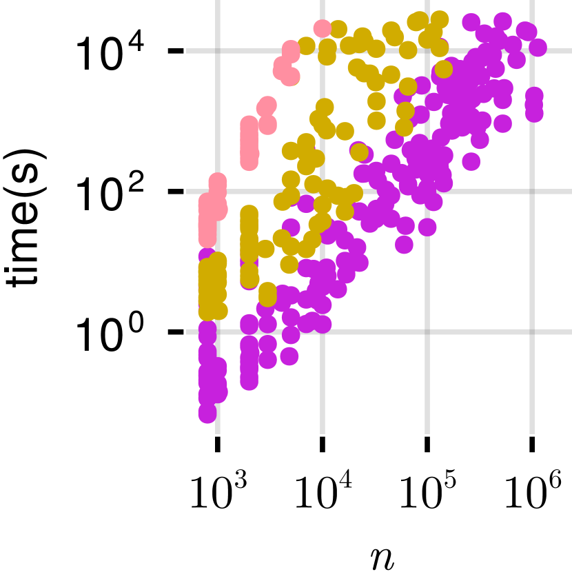
(c) Cut Norm Runtime by Prob. Size

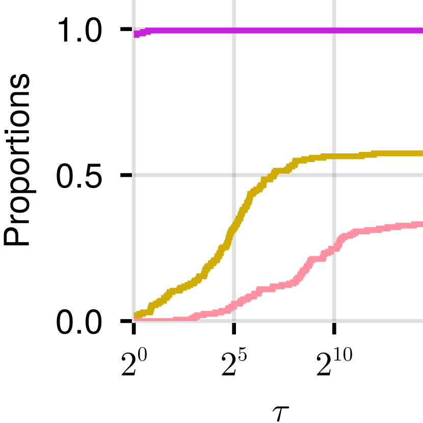
(d) Cut Norm Runtime Perf. Prof.

Figure 3: Results on Lovàsz Theta and Cut Norm.

5.5 Lovàsz Theta

The Lovàsz theta function [42] of an undirected graph $G=(V,E)$, $\vartheta(G)$, can be computed by

$$\vartheta(G)=\mathop{\text{maximize}}_{\bm{X}\succeq 0}\;\bm{\mathrm{1}}^{T}\bm{X}\bm{\mathrm{1}}\;\mathop{\text{subject to}}\;\text{Tr}(\bm{X})=1,\bm{X}_{ij}=0\ \text{for all }ij\in E.$$ (Lovàsz Theta)

Computing $\vartheta(G)$ reveals key characteristics of a graph because of the sandwich result $\alpha(G)\leqslant\vartheta(G)\leqslant\chi(\bar{G})$ where $\alpha(G)$ is the size of the maximum independent set in $G$ and $\chi(\bar{G})$ is the chromatic number of the complement of $G$. We pick the trace bound $\alpha$ as $1$ for SDPLR+ and SketchyCGAL. Figure 3 summarizes results and shows that SketchyCGAL is often faster than SDPLR+ for this SDP.

5.6 Cut Norm

The cut norm is relevant to a variety of graph and matrix problems [4, 25]. For any $\bm{A}\in\R^{m\times n}$, its cut norm is defined as $\|\bm{A}\|_{\text{cut}}=\mathop{\text{max}}_{S\subseteq[m],T\subseteq[n]}|\sum_{i\in S}\sum_{j\in T}\bm{A}_{ij}|$. While computing the cut norm is not tractable, Alon and Naor gave a 0.56-approximation algorithm based on solving the following SDP and rounding its solution [3]

$$\mathop{\text{maximize}}_{\bm{X}}\;\tfrac{1}{2}\langle\bigl{[}\begin{smallmatrix}\bm{\mathrm{0}}&\bm{A}\\ \bm{A}^{T}&\bm{\mathrm{0}}\end{smallmatrix}\bigr{]},\bm{X}\rangle\;\mathop{\text{subject to}}\;\mathop{\text{diag}}(\bm{X})=\bm{\mathrm{1}}.$$ (Cut Norm)

We compare SDPLR+ against SketchyCGAL and CSDP. We pick the trace bound $\alpha$ as $m+n$ for SDPLR+ and SketchyCGAL. The results are summarized in Figure 3, which show that SDPLR+ is often much faster than SketchyCGAL for this SDP.

5.7 Ablation studies

In the appendix, we do two ablation studies. Appendix F shows how the changes in SDPLR+ compare to SDPLR in runtime. As would be expected, SDPLR+ is faster on the vast majority of instances. Appendix G studies a number of solvers with a fixed rank or fixed sketch size. This eliminates the dynamic behavior in some of the solvers.

6 Limitations and Conclusions

Limitations

Empirical studies of solvers are always challenging. Do we pick optimal parameters for each solver via hyperparameter search or results with default options? In this case, we chose to use default options. To address some of the limitations that this imposes, we did a fixed rank study in Appendix G that compares the solvers in a directly comparable parameter regime. Performance profile plots also can be misleading [28]. This is why we show both runtime and size as well – which typically highlights the same trend. For one recent solver, we were unable to obtain an implementation to compare [44] and data from the paper is from a very different accuracy regime. For another recent solver [5], we encountered issues when trying to complete a full evaluation. In this case, we present a comparison against values from their paper in Appendix E.

Although we target trace bounded SDPs, this is a very general setting as many problems have easy to compute bounds on the maximum possible trace of the solution. For those that don’t, doubling approaches could be used to scale the upper bound through a variety of choices.

Conclusion

The research field has made tremendous progress on solving large SDPs. This paper continues this thread of research and proposes a new solver for trace-bounded SDPs that adds a suboptimality bound to SDPLR to improve it into the new solver SDPLR+. We were impressed at the improvement from this straightforward improvement to the solver. This further supports the idea that there remains large potential speed improvements in SDP solvers.

Appendix A Example for strong duality

We give one example to help understand why a trace bound gives strong duality. One classical example for demonstrating the duality gap may exist between (SDP) and (SDD) is

$$\mathop{\text{min}} \quad y_{1}$$

s.t. $$\quad\begin{bmatrix}0&y_{1}&0\\ y_{1}&y_{2}&0\\ 0&0&y_{1}+1\end{bmatrix}\succeq 0.$$

Because any principal submatrix of a symmetric positive semidefinite matrix has to be positive semidefinite, we get $y_{1}^{2}\leqslant 0$ and the optimum of it is 0. Writing it in the standard (SDP) form gives us

$$\mathop{\text{minimize}}_{\bm{X}\succeq 0} \quad\langle\Bigl{[}\begin{smallmatrix}0&\frac{1}{2}&0\\ \frac{1}{2}&0&0\\ 0&0&0\end{smallmatrix}\Bigr{]},\bm{X}\rangle$$ (Example SDP)

$$\mathop{\text{subject to}} \quad\langle\Bigl{[}\begin{smallmatrix}0&0&1\\ 0&0&0\\ 1&0&0\end{smallmatrix}\Bigr{]},\bm{X}\rangle=0,\langle\Bigl{[}\begin{smallmatrix}0&0&0\\ 0&0&1\\ 0&1&0\end{smallmatrix}\Bigr{]},\bm{X}\rangle=0,\langle\Bigl{[}\begin{smallmatrix}1&0&0\\ 0&0&0\\ 0&0&0\end{smallmatrix}\Bigr{]},\bm{X}\rangle=0,\langle\Bigl{[}\begin{smallmatrix}0&1&0\\ 1&0&0\\ 0&0&-2\end{smallmatrix}\Bigr{]},\bm{X}\rangle=-2,$$

whose dual is

$$\mathop{\text{max}}_{\lambda\in\R^{4}} \quad-2\lambda_{4}$$ (Example SDD)

s.t. $$\quad\begin{bmatrix}-\lambda_{3}&\frac{1}{2}-\lambda_{4}&-\lambda_{1}\\ \frac{1}{2}-\lambda_{4}&0&-\lambda_{2}\\ -\lambda_{1}&-\lambda_{2}&2\lambda_{4}\end{bmatrix}\succeq 0.$$

Similarly, we have $(\frac{1}{2}-\lambda_{4})^{2}\leqslant 0$, which leads to $\lambda_{4}=\frac{1}{2}$ and (Example SDD) having optimum $-1$. A duality gap does exist.

However, if we add one trace bound $\text{Tr}(\bm{X})\leqslant 1$ to (Example SDP), its optimum stays unchanged and its dual becomes

$$\mathop{\text{max}}_{\lambda\in\R^{4}}-2\lambda_{4}+\mathop{\text{min}}\left\{0,\lambda_{\mathop{\text{min}}}\left(\begin{bmatrix}-\lambda_{3}&\frac{1}{2}-\lambda_{4}&-\lambda_{1}\\ \frac{1}{2}-\lambda_{4}&0&-\lambda_{2}\\ -\lambda_{1}&-\lambda_{2}&2\lambda_{4}\end{bmatrix}\right)\right\},$$

whose optimum is also 0 (plug in $\lambda_{1}=\lambda_{2}=\lambda_{3}=0,\lambda_{4}=-\frac{1}{2}$).

Appendix B Connections between Different Suboptimality Bounds

Here for completeness, we include a concise proof for the surrogate duality bound from [69]. We slightly adjust their proof because the compact domain we consider is $\Delta_{\alpha}=\{\bm{X}\succeq 0\mathrel{\mathop{\mathchar 58\relax}}\text{Tr}(\bm{X})\leqslant\alpha\}$, which is slightly different from $\{\bm{X}\succeq 0\mathrel{\mathop{\mathchar 58\relax}}\text{Tr}(\bm{X})=\alpha\}$. The adjustment is straightforward.

For convenience, we let $p(\bm{X})\coloneqq\mathcal{A}(\bm{X})-\bm{\mathrm{b}}$ denote the primal violation of $\bm{X}$. They consider the following augmented Lagrangian

$$f(\bm{X})=\langle\bm{C},\bm{X}\rangle-\bm{\mathrm{\lambda}}^{T}p(\bm{X})+\frac{\sigma}{2}\|p(\bm{X})\|^{2}$$ (5)

and the corresponding minimization problem

$$\mathop{\text{minimize}}_{\bm{X}\in\Delta_{\alpha}}\;f(\bm{X})$$

where $\sigma>0$. Because (5) is convex, we have the following surrogate duality bound by applying the surrogate duality bound in Frank-Wolfe [31] to $f$,

$$\mathop{\text{max}}_{\bm{H}\in\Delta_{\alpha}}\langle\nabla f(\bm{X}),\bm{X}-\bm{H}\rangle\geqslant f(\bm{X})-\mathop{\text{min}}_{\bm{Z}\in\Delta_{\alpha}}f(\bm{Z})\geqslant f(\bm{X})-f(\bm{X}^{*})=f(\bm{X})-\langle\bm{C},\bm{X}^{*}\rangle$$ (6)

where $\bm{X}^{*}$ is one optimal solution for (Trace-Bounded SDP). The last inequality is because $f(\bm{X}^{*})\geqslant\mathop{\text{min}}_{\bm{Z}\in\Delta_{\alpha}}f(\bm{Z})$ and the last equality is due to $\bm{X}^{*}$ is feasible, i.e. $p(\bm{X}^{*})=0$.

Let $\bm{\mathrm{\lambda}}^{\prime}=\bm{\mathrm{\lambda}}-\sigma p(\bm{X})$, we note that $\nabla f(\bm{X})=\bm{C}-\mathcal{A}^{*}(\bm{\mathrm{\lambda}}^{\prime})$ and

$$\mathop{\text{max}}_{\bm{H}\in\Delta_{\alpha}}\langle\nabla f(\bm{X}),-\bm{H}\rangle=-\mathop{\text{min}}_{\bm{H}\in\Delta_{\alpha}}\langle\nabla f(\bm{X}),\bm{H}\rangle=-\alpha\mathop{\text{min}}\{0,\lambda_{\mathop{\text{min}}}(\nabla f(\bm{X}))\},$$

hence we have

$$\mathop{\text{max}}_{\bm{H}\in\Delta_{\alpha}}\langle\nabla f(\bm{X}),\bm{X}-\bm{H}\rangle=\langle\bm{C}-\mathcal{A}^{*}(\bm{\mathrm{\lambda}}^{\prime}),\bm{X}\rangle-\alpha\mathop{\text{min}}\{0,\lambda_{\mathop{\text{min}}}(\nabla f(\bm{X}))\}$$ (7)

Also we can rewrite $f$ as

$$f(\bm{X})=\langle\bm{C},\bm{X}\rangle-(\bm{\mathrm{\lambda}}^{\prime})^{T}p(\bm{X})-\frac{\sigma}{2}\|p(\bm{X})\|^{2}.$$ (8)

Thus we have

$$\quad\langle\bm{C},\bm{X}\rangle-\langle\bm{C},\bm{X}^{*}\rangle$$

$$=f(\bm{X})-\langle\bm{C},\bm{X}^{*}\rangle+(\bm{\mathrm{\lambda}}^{\prime})^{T}p(\bm{X})+\frac{\sigma}{2}\|p(\bm{X})\|^{2}$$

$$\leqslant\mathop{\text{max}}_{\bm{H}\in\Delta_{\alpha}}\langle\nabla f(\bm{X}),\bm{X}-\bm{H}\rangle+(\bm{\mathrm{\lambda}}^{\prime})^{T}p(\bm{X})+\frac{\sigma}{2}\|p(\bm{X})\|^{2}$$

$$=\langle\bm{C}-\mathcal{A}^{*}(\bm{\mathrm{\lambda}}^{\prime}),\bm{X}\rangle-\alpha\mathop{\text{min}}\{\lambda_{\mathop{\text{min}}}(\bm{C}-\calA^{*}(\bm{\mathrm{\lambda}}^{\prime})),0\}+(\bm{\mathrm{\lambda}}^{\prime})^{T}p(\bm{X})+\frac{\sigma}{2}\|p(\bm{X})\|^{2}$$

$$=\langle\bm{C},\bm{X}\rangle-\bm{\mathrm{b}}^{T}\bm{\mathrm{\lambda}}^{\prime}-\alpha\mathop{\text{min}}\{\lambda_{\mathop{\text{min}}}(\bm{C}-\calA^{*}(\bm{\mathrm{\lambda}}^{\prime})),0\}+\frac{\sigma}{2}\|p(\bm{X})\|^{2}$$ (9)

where the first equality is due to (8), the first inequality is due to (6), the second equality is due to (7) and the third equality is due to $\langle\mathcal{A}^{*}(\bm{\mathrm{\lambda}}^{\prime}),\bm{X}\rangle=(\bm{\mathrm{\lambda}}^{\prime})^{T}\mathcal{A}(\bm{X})=(\bm{\mathrm{\lambda}}^{\prime})^{T}(p(\bm{X})+\bm{\mathrm{b}})$.

We can see (B) has a clear relation to (1) as $\bm{\mathrm{\lambda}}^{\prime}$ is feasible for (Trace-bounded SDD). Also we notice by (1), the term $\frac{\sigma}{2}\|p(\bm{X})\|^{2}$ is unnecessary and will result in a worse bound. Interestingly, $\bm{\mathrm{\lambda}}^{\prime}$ is exactly the updated dual in the classical augmented Lagrangian framework.

Appendix C The SDPLR+ algorithm

We give the pseudocode of the core algorithm of SDPLR+. We use $\eta,\omega,\xi$ to denote the stationarity tolerance, primal infeasibility tolerance and suboptimality tolerance respectively. We let $\omega^{*},\xi^{*}$ denote the desired primal infeasibility and suboptimality tolerances input by the user. We use $\lambda$ to denote the Lagrangian multipliers estimated and $\sigma$ denote the smoothing parameter in the augmented Lagrangian method. The augmented Lagrangian function is

$$f(\bm{Y})=\langle\bm{C},\bm{Y}\bm{Y}^{T}\rangle-\bm{\mathrm{\lambda}}^{T}(\mathcal{A}(\bm{X})-\bm{\mathrm{b}})+\frac{\sigma}{2}\|\mathcal{A}(\bm{X})-\bm{\mathrm{b}}\|^{2}.$$ (10)

1:$\bm{C},\mathcal{A},\bm{\mathrm{b}},\omega^{*},\xi^{*},\alpha,r,\bm{Y},\bm{\mathrm{\lambda}}$.

2:$\bm{Y}$ satisfying desired primal infeasibility and suboptimality precision

3:$\sigma=2,\eta=\frac{1}{\sigma},\omega=\frac{1}{\sigma^{0.1}},cnt=4$

4:repeat

5:     Use L-BFGS to find a new $\bm{Y}$ such that $\|\nabla f(\bm{Y})\|_{F}\leqslant\eta(1+\|\bm{C}\|_{F})$ where $f$ is defined in Equation (10).

6:     if $\|\mathcal{A}(\bm{Y}\bm{Y}^{T})-\bm{\mathrm{b}}\|\leqslant\omega(1+\|\bm{\mathrm{b}}\|)$ then

7:         if $\|\mathcal{A}(\bm{Y}\bm{Y}^{T})-\bm{\mathrm{b}}\|\leqslant\omega^{*}(1+\|\bm{\mathrm{b}}\|)$ then

8:              if $\langle\bm{C},\bm{Y}\bm{Y}^{T}\rangle-\bm{\mathrm{\lambda}}^{T}\bm{\mathrm{b}}-\alpha\{\lambda_{\mathop{\text{min}}}(\bm{C}-\calA^{*}(\bm{\mathrm{\lambda}})),0\}\leqslant\xi^{*}(1+|\langle\bm{C},\bm{Y}\bm{Y}^{T}\rangle|)$ then

9:                  Break

10:              else

11:                  $cnt=cnt-1$

12:              end if

13:         end if

14:         $\bm{\mathrm{\lambda}}=\bm{\mathrm{\lambda}}-\sigma(\mathcal{A}(\bm{Y}\bm{Y}^{T})-\bm{\mathrm{b}})$

15:         $\eta=\frac{\eta}{\sigma},\omega=\frac{\omega}{\sigma^{0.9}}$

16:     else

17:         $\sigma=2\sigma,\eta=\frac{1}{\sigma},\omega=\frac{1}{\sigma^{0.1}}$

18:     end if

19:     if $cnt=0$ then

20:         $r=\mathop{\text{min}}\{2r,\lfloor\sqrt{2m}+1\rfloor\}$, regenerate $\bm{Y}$ and $\bm{\mathrm{\lambda}}$ accordingly, set $cnt=4$.

21:     end if

22:until $\|\mathcal{A}(\bm{Y}\bm{Y}^{T})-\bm{\mathrm{b}}\|\leqslant\omega^{*}(1+\|\bm{\mathrm{b}}\|)$ and $(\langle\bm{C},\bm{Y}\bm{Y}^{T}\rangle-\langle\bm{C},\bm{X}^{*}\rangle)\leqslant\xi^{*}(1+|\langle\bm{C},\bm{Y}\bm{Y}^{T}\rangle|)$

Algorithm 1 Pseudocode of the core algorithm of SDPLR+

We generate the initial $\bm{Y}$ and $\bm{\mathrm{\lambda}}$ randomly. The pseudocode is summarized in Algorithm 1. The main difference with SDPLR is that we applied the two techniques we introduced. Also, we customized the augmented Lagrangian update rules, we adopted one from [46].

Appendix D More Implementation and Experiment Details

In this section, we introduce more details about all the implementations and experiments. We first introduce more dataset details and statistics. Then we introduce the experiment compute resources.

D.1 Dataset Details

For Gset, we include all the graphs. We pick the following two groups of graphs from the SNAP dataset [37].

• 4 web graphs web-BerkStan, web-Google, web-Stanford [39], web-NotreDame [2].

• 11 community graphs ca-AstroPh, ca-CondMat, ca-GrQc, ca-HepPh, ca-HepTh [38], com-youtube, com-dblp, com-amazon [67], email-Enron [33], musae-facebook [53], feather-deezer-social [52].

For DIMACS10, for the interest of benchmarking time, we sort graphs by the number of vertices they contain and keep the first 116 graphs. The largest one rgg_n_2_20_s0 has $n=1048576$.

We provide some statistics of these 202 graphs, which are summarized in Figure 5.

D.2 Experiments Compute Resources

We ran our experiments on three servers, two of which had the same configuration.

• One server with 64 cores and each core has two threads. The CPU model is Intel(R) Xeon(R) CPU E7-8867 v3 @ 2.50GHz.

• Two servers with 28 cores each and each core has two threads. The CPU model is Intel(R) Xeon(R) CPU E5-2690 v4 @ 2.60GHz.

In our experiments, we let each solver solve each problem instance using only one thread. We use GNU Parallel [60] to parallelize the benchmarking and timeout each solver after running for 8 hours by setting ----timeout 28800. We limit the total RAM access to 16GB via ulimit -d 16777216.

D.3 Solver-Specific Implementation Details

CSDP

CSDP has slightly different quality measures. First of all, the dual problem that CSDP tackles is slightly different, which is

$$\mathop{\text{max}}_{\bm{\mathrm{\lambda}},\bm{Z}\succeq 0}\;\bm{\mathrm{\lambda}}^{T}\bm{\mathrm{b}}\;\mathop{\text{subject to}}\;\bm{C}-\calA^{*}(\bm{\mathrm{\lambda}})=\bm{Z}.$$ (11)

Besides (Primal Infeasibility), they have two other quality measures for dual and the duality gap $\displaystyle\frac{\|\mathcal{A}^{*}(\bm{\mathrm{\lambda}})-\bm{C}-\bm{Z}\|_{F}}{1+\|\bm{C}\|}$ (Dual Infeasibility) $\displaystyle\frac{\langle\bm{X},\bm{Z}\rangle}{1+|\langle\bm{C},\bm{X}\rangle|+|\bm{\mathrm{\lambda}}^{T}\bm{\mathrm{b}}|}.$ (Relative Duality Gap)

SDPLR+

We implement SDPLR+ in Julia [10]. The code began as a port of the SDPLR library.

Appendix E Comparison against USBS

While we did not find the code for USBS [5] in time to run a full comparison, we are able to do a preliminary comparison against the data reported in their paper. Specifically, we extract data from their performance figures via the tool WebPlotDigitizer [51]. The results are shown in Table 1. We were unable to learn if their solver was run with any multithreading. It was also run with a lower accuracy than we run SDPLR+. Nonetheless, we see that SDPLR+ is faster on most problems.

Table 1: A comparison against USBS [5] using results from their paper. We were unable to run an evaluation of USBS in time, but these results indicate that SDPLR+ is faster on many problems by a considerable margin, albeit these are from different systems.

Problem/Time (s)	fe_sphere	hi2010	fe_body	me2010	fe_tooth	598a	144	auto
USBS/warm $(\varepsilon=10^{-1})$	31	125	273	417	348	636	810	3444
SDPLR+ $(\varepsilon=10^{-2})$	7	160	38	613	43	192	170	634

Appendix F Ablation Study: SDPLR vs. SDPLR+

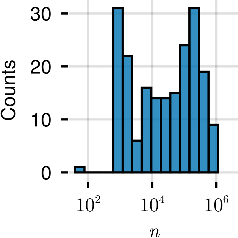
(a) Stats of $n$

(b) Stats of Non-zeros

Figure 4: Statistics of $n$ and the number of non-zeros of 202 matrices we test on.

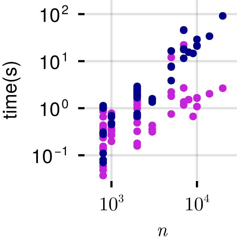
(c) Runtime by Size

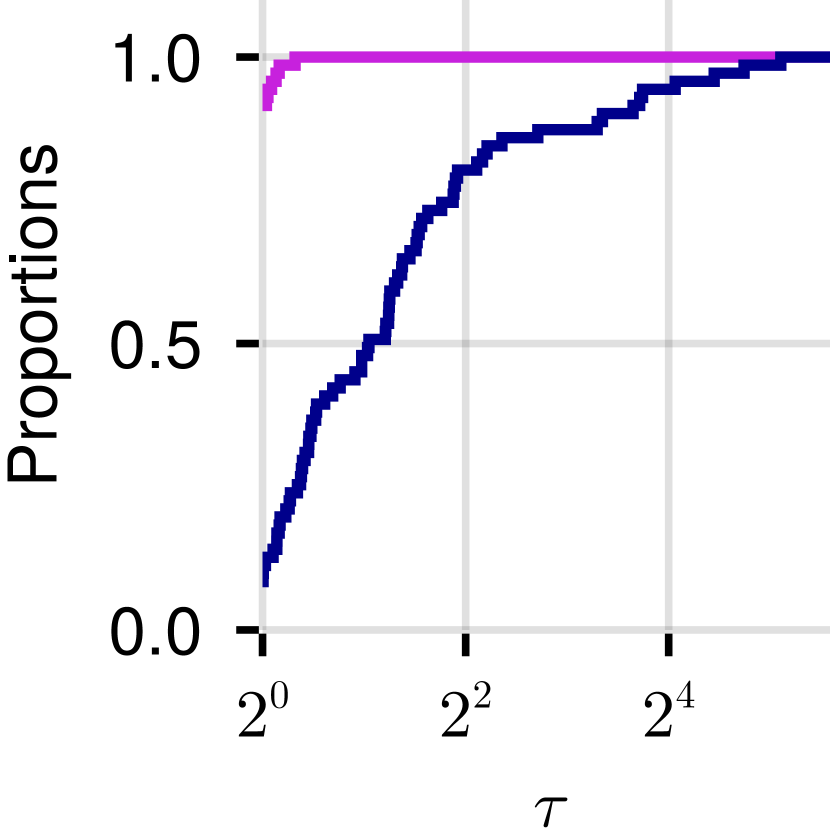
(d) Runtime Perf. Prof.

Figure 5: Comparing SDPLR+ against SDPLR for solving Max Cut on Gset graphs.

We perform some simple comparison experiments to demonstrate SDPLR+ is faster than the original SDPLR. We let them both solve Max Cut on Gset, which contains 71 small and moderate graphs. We terminate SDPLR+ once both (Primal Infeasibility) and (Suboptimality) are smaller than $\varepsilon$ and SDPLR once (Primal Infeasibility) is smaller than $\varepsilon$. We slightly modified SDPLR to compute the (Primal Infeasibility) in Euclidean scaling for fair comparison. The results are summarized in Figure 5. As we can see, SDPLR+ is faster on the vast majority of instances.

Appendix G Ablation Study: Impact of Rank Parameter and Sketch Size

Recall that SDPLR+ and Manopt have a parameter $r$ controls the rank of the low-rank factors they optimize, and SketchyCGAL has a parameter $R$ controls the size of the sketch $\bm{S}\in\R^{n\times R}$ they store. We compare the performance of SDPLR+, Manopt and SketchyCGAL on Max Cut with various rank parameters and sketch size and explore how these parameters affect their convergence speed to moderately accurate solutions. For simplicity, we let the rank parameter and the sketch size be the same. We slightly modified the Max Cut code of Manopt to achieve different ranks. The results are summarized in Figure 6.

(a) Runtime by Size Rank 50

(b) Runtime Perf. Prof. Rank 50

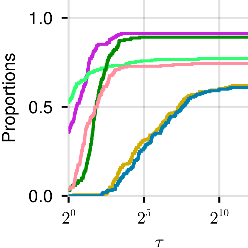
(c) Runtime Perf. Prof. for both 10, 50

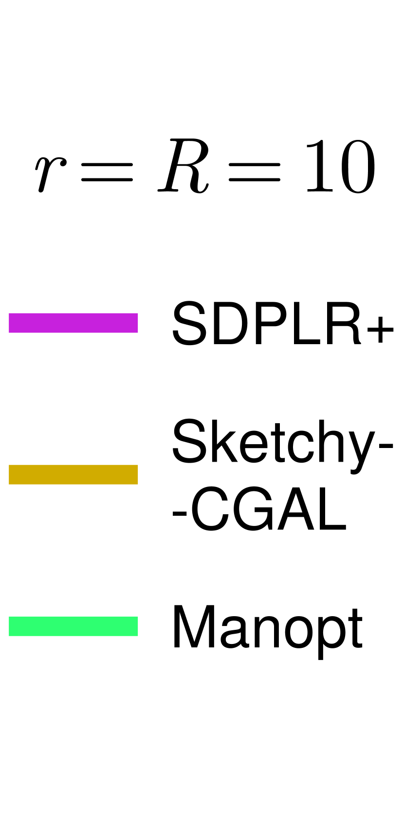
Figure 6: Results on investigation of rank parameters and sketch sizes. We observe that if we decrease the rank parameter used in Manopt, it has comparable performance against SDPLR+, although SDPLR+ remains the fastest solver. When $r=R=10$, the runtime by size and the runtime performance plot are similar to 6(a) and 6(b), so we omit them. From the performance plot 6(c), we can see that in general, a higher rank parameter or sketch size will result in longer running time for moderate accuracy.

References

- Absil et al. [2007] P-A Absil, Christopher G Baker, and Kyle A Gallivan. Trust-region methods on riemannian manifolds. Foundations of Computational Mathematics, 7:303–330, 2007.
- Albert et al. [1999] Réka Albert, Hawoong Jeong, and Albert-László Barabási. Diameter of the World-Wide Web. Nature, 401(6749):130–131, September 1999. ISSN 1476-4687. doi: 10.1038/43601.
- Alon and Naor [2004] Noga Alon and Assaf Naor. Approximating the cut-norm via Grothendieck’s inequality. In Proceedings of the Thirty-Sixth Annual ACM Symposium on Theory of Computing, STOC ’04, pages 72–80, New York, NY, USA, June 2004. Association for Computing Machinery. ISBN 978-1-58113-852-8. doi: 10.1145/1007352.1007371.
- Alon et al. [1994] Noga Alon, Richard A Duke, Hanno Lefmann, Vojtech Rodl, and Raphael Yuster. The algorithmic aspects of the regularity lemma. Journal of Algorithms, 16(1):80–109, 1994.
- Angell and McCallum [2024] Rico Angell and Andrew McCallum. Fast, scalable, warm-start semidefinite programming with spectral bundling and sketching, 2024.
- Arora et al. [2009] Sanjeev Arora, Satish Rao, and Umesh Vazirani. Expander flows, geometric embeddings and graph partitioning. Journal of the ACM, 56(2):5:1–5:37, April 2009. ISSN 0004-5411. doi: 10.1145/1502793.1502794.
- Balan et al. [2009] Radu Balan, Bernhard G Bodmann, Peter G Casazza, and Dan Edidin. Painless reconstruction from magnitudes of frame coefficients. Journal of Fourier Analysis and Applications, 15(4):488–501, 2009.
- Bansal et al. [2004] Nikhil Bansal, Avrim Blum, and Shuchi Chawla. Correlation clustering. Machine learning, 56:89–113, 2004.
- Barvinok [1995] A. I. Barvinok. Problems of distance geometry and convex properties of quadratic maps. Discrete & Computational Geometry, 13(2):189–202, March 1995. ISSN 1432-0444. doi: 10.1007/BF02574037.
- Bezanson et al. [2017] Jeff Bezanson, Alan Edelman, Stefan Karpinski, and Viral B. Shah. Julia: A Fresh Approach to Numerical Computing. SIAM Review, 59(1):65–98, January 2017. ISSN 0036-1445. doi: 10.1137/141000671.
- Borchers [1999] Brian Borchers. CSDP, A C library for semidefinite programming. Optimization Methods and Software, 11(1-4):613–623, January 1999. ISSN 1055-6788. doi: 10.1080/10556789908805765.
- Boumal et al. [2018] Nicolas Boumal, Vladislav Voroninski, and Afonso S. Bandeira. The non-convex Burer-Monteiro approach works on smooth semidefinite programs, April 2018.
- Boumal et al. [2020] Nicolas Boumal, Vladislav Voroninski, and Afonso S. Bandeira. Deterministic Guarantees for Burer-Monteiro Factorizations of Smooth Semidefinite Programs. Communications on Pure and Applied Mathematics, 73(3):581–608, 2020. ISSN 1097-0312. doi: 10.1002/cpa.21830.
- Boyd [1994] Stephen P. Boyd, editor. Linear Matrix Inequalities in System and Control Theory. Number 15 in SIAM Studies in Applied Mathematics. Society for Industrial and Applied Mathematics, Philadelphia, Pa, 1994. ISBN 978-0-89871-334-3 978-0-89871-485-2.
- Burer and Choi [2006] Samuel Burer and Changhui Choi. Computational enhancements in low-rank semidefinite programming. Optimization Methods and Software, 21(3):493–512, June 2006. ISSN 1055-6788. doi: 10.1080/10556780500286582.
- Burer and Monteiro [2003] Samuel Burer and Renato D.C. Monteiro. A nonlinear programming algorithm for solving semidefinite programs via low-rank factorization. Mathematical Programming, 95(2):329–357, February 2003. ISSN 1436-4646. doi: 10.1007/s10107-002-0352-8.
- Burer and Monteiro [2005] Samuel Burer and Renato D.C. Monteiro. Local Minima and Convergence in Low-Rank Semidefinite Programming. Mathematical Programming, 103(3):427–444, July 2005. ISSN 1436-4646. doi: 10.1007/s10107-004-0564-1.
- Candès and Recht [2012] Emmanuel Candès and Benjamin Recht. Exact matrix completion via convex optimization. Communications of the ACM, 55(6):111–119, June 2012. ISSN 0001-0782. doi: 10.1145/2184319.2184343.
- Cifuentes [2021] Diego Cifuentes. On the Burer–Monteiro method for general semidefinite programs. Optimization Letters, 15(6):2299–2309, September 2021. ISSN 1862-4480. doi: 10.1007/s11590-021-01705-4.
- Cifuentes and Moitra [2022] Diego Cifuentes and Ankur Moitra. Polynomial time guarantees for the Burer-Monteiro method. In Advances in Neural Information Processing Systems, October 2022.
- Davis and Hu [2011] Timothy A. Davis and Yifan Hu. The university of Florida sparse matrix collection. ACM Transactions on Mathematical Software, 38(1):1:1–1:25, December 2011. ISSN 0098-3500. doi: 10.1145/2049662.2049663.
- Ding et al. [2020] Lijun Ding, Alp Yurtsever, Volkan Cevher, Joel A. Tropp, and Madeleine Udell. An Optimal-Storage Approach to Semidefinite Programming using Approximate Complementarity, June 2020.
- Dolan and Moré [2002] Elizabeth D Dolan and Jorge J Moré. Benchmarking optimization software with performance profiles. Mathematical programming, 91:201–213, 2002.
- Frieze and Jerrum [1997] A. Frieze and M. Jerrum. Improved approximation algorithms for MAXk-CUT and MAX BISECTION. Algorithmica, 18(1):67–81, May 1997. ISSN 1432-0541. doi: 10.1007/BF02523688.
- Frieze and Kannan [1999] Alan Frieze and Ravi Kannan. Quick approximation to matrices and applications. Combinatorica, 19(2):175–220, 1999.
- Garey et al. [1976] M.R. Garey, D.S. Johnson, and L. Stockmeyer. Some simplified np-complete graph problems. Theoretical Computer Science, 1(3):237–267, 1976. ISSN 0304-3975. doi: https://doi.org/10.1016/0304-3975(76)90059-1. URL https://www.sciencedirect.com/science/article/pii/0304397576900591.
- Goemans and Williamson [1995] Michel X. Goemans and David P. Williamson. Improved approximation algorithms for maximum cut and satisfiability problems using semidefinite programming. Journal of the ACM, 42(6):1115–1145, November 1995. ISSN 0004-5411. doi: 10.1145/227683.227684.
- Gould and Scott [2016] Nicholas Gould and Jennifer Scott. A note on performance profiles for benchmarking software. ACM Transactions on Mathematical Software, 43(2):1–5, August 2016. ISSN 1557-7295. doi: 10.1145/2950048. URL http://dx.doi.org/10.1145/2950048.
- Hazan [2008] Elad Hazan. Sparse Approximate Solutions to Semidefinite Programs. In Eduardo Sany Laber, Claudson Bornstein, Loana Tito Nogueira, and Luerbio Faria, editors, LATIN 2008: Theoretical Informatics, Lecture Notes in Computer Science, pages 306–316, Berlin, Heidelberg, 2008. Springer. ISBN 978-3-540-78773-0. doi: 10.1007/978-3-540-78773-0_27.
- Huang et al. [2023] Yufan Huang, C. Seshadhri, and David F. Gleich. Theoretical Bounds on the Network Community Profile from Low-rank Semi-definite Programming. In Proceedings of the 40th International Conference on Machine Learning, pages 13976–13992. PMLR, July 2023.
- Jaggi [2013] Martin Jaggi. Revisiting Frank-Wolfe: Projection-free sparse convex optimization. In Sanjoy Dasgupta and David McAllester, editors, Proceedings of the 30th International Conference on Machine Learning, volume 28 of Proceedings of Machine Learning Research, pages 427–435, Atlanta, Georgia, USA, 17–19 Jun 2013. PMLR. URL https://proceedings.mlr.press/v28/jaggi13.html.
- Kleinman and Athans [1968] D. Kleinman and M. Athans. The design of suboptimal linear time-varying systems. IEEE Transactions on Automatic Control, 13(2):150–159, 1968. doi: 10.1109/TAC.1968.1098852.
- Klimt and Yang [2004] Bryan Klimt and Yiming Yang. Introducing the Enron Corpus. In International Conference on Email and Anti-Spam, 2004.
- Kuczyński and Woźniakowski [1992] J. Kuczyński and H. Woźniakowski. Estimating the Largest Eigenvalue by the Power and Lanczos Algorithms with a Random Start. SIAM Journal on Matrix Analysis and Applications, 13(4):1094–1122, October 1992. ISSN 0895-4798. doi: 10.1137/0613066.
- Kulis et al. [2007] Brian Kulis, Arun C. Surendran, and John C. Platt. Fast low-rank semidefinite programming for embedding and clustering. In Marina Meila and Xiaotong Shen, editors, Proceedings of the Eleventh International Conference on Artificial Intelligence and Statistics, volume 2 of Proceedings of Machine Learning Research, pages 235–242, San Juan, Puerto Rico, 21–24 Mar 2007. PMLR. URL https://proceedings.mlr.press/v2/kulis07a.html.
- Lemon et al. [2016] Alex Lemon, Anthony Man-Cho So, and Yinyu Ye. Low-Rank Semidefinite Programming: Theory and Applications. Foundations and Trends® in Optimization, 2(1-2):1–156, 2016. ISSN 2167-3888, 2167-3918. doi: 10.1561/2400000009.
- Leskovec and Krevl [2014] Jure Leskovec and Andrej Krevl. SNAP Datasets: Stanford large network dataset collection. http://snap.stanford.edu/data, June 2014.
- Leskovec et al. [2007] Jure Leskovec, Jon Kleinberg, and Christos Faloutsos. Graph evolution: Densification and shrinking diameters. ACM Transactions on Knowledge Discovery from Data, 1(1):2–es, March 2007. ISSN 1556-4681. doi: 10.1145/1217299.1217301.
- Leskovec et al. [2008] Jure Leskovec, Kevin J. Lang, Anirban Dasgupta, and Michael W. Mahoney. Community Structure in Large Networks: Natural Cluster Sizes and the Absence of Large Well-Defined Clusters, October 2008.
- Liu and Boumal [2019] Changshuo Liu and Nicolas Boumal. Simple algorithms for optimization on Riemannian manifolds with constraints, April 2019.
- Liu and Nocedal [1989] Dong C Liu and Jorge Nocedal. On the limited memory bfgs method for large scale optimization. Mathematical programming, 45(1):503–528, 1989.
- Lovász [1979] László Lovász. On the shannon capacity of a graph. IEEE Transactions on Information theory, 25(1):1–7, 1979.
- Majumdar et al. [2019] Anirudha Majumdar, Georgina Hall, and Amir Ali Ahmadi. A Survey of Recent Scalability Improvements for Semidefinite Programming with Applications in Machine Learning, Control, and Robotics, December 2019.
- Monteiro et al. [2024] Renato DC Monteiro, Arnesh Sujanani, and Diego Cifuentes. A low-rank augmented lagrangian method for large-scale semidefinite programming based on a hybrid convex-nonconvex approach. arXiv preprint arXiv:2401.12490, 2024.
- Nesterov [2011] Yurii Nesterov. Barrier subgradient method. Mathematical Programming, 127(1):31–56, March 2011. ISSN 0025-5610, 1436-4646. doi: 10.1007/s10107-010-0421-3.
- Nocedal and Wright [2006] Jorge Nocedal and Stephen J. Wright. Numerical Optimization. Springer Series in Operations Research. Springer, New York, 2nd ed edition, 2006. ISBN 978-0-387-30303-1.
- O’Carroll et al. [2022] Liam O’Carroll, Vaidehi Srinivas, and Aravindan Vijayaraghavan. The Burer-Monteiro SDP method can fail even above the Barvinok-Pataki bound. In Advances in Neural Information Processing Systems, October 2022.
- Orban [2019] Dominique Orban. Benchmarkprofiles.jl, 2019. URL https://zenodo.org/record/4630955.
- Pataki [1998] Gábor Pataki. On the Rank of Extreme Matrices in Semidefinite Programs and the Multiplicity of Optimal Eigenvalues. Mathematics of Operations Research, 23(2):339–358, 1998. ISSN 0364-765X.
- Pham et al. [2023] Chi Bach Pham, Wynita Griggs, and James Saunderson. A Scalable Frank-Wolfe-Based Algorithm for the Max-Cut SDP. In Proceedings of the 40th International Conference on Machine Learning, pages 27822–27839. PMLR, July 2023.
- Rohatgi [2024] A. Rohatgi. Webplotdigitizer version 4.0, 2024. URL https://github.com/automeris-io/WebPlotDigitizer.
- Rózemberczki and Sarkar [2020] Benedek Rózemberczki and Rik Sarkar. Characteristic Functions on Graphs: Birds of a Feather, from Statistical Descriptors to Parametric Models. In Proceedings of the 29th ACM International Conference on Information & Knowledge Management. ACM Association for Computing Machinery, October 2020. doi: 10.1145/3340531.3411866.
- Rozemberczki et al. [2021] Benedek Rozemberczki, Carl Allen, and Rik Sarkar. Multi-Scale attributed node embedding. Journal of Complex Networks, 9(2):cnab014, April 2021. ISSN 2051-1329. doi: 10.1093/comnet/cnab014.
- Sanchis [1989] Laura A Sanchis. Multiple-way network partitioning. IEEE Transactions on Computers, 38(1):62–81, 1989.
- Shinde et al. [2021a] Nimita Shinde, Vishnu Narayanan, and James Saunderson. Memory-Efficient Structured Convex Optimization via Extreme Point Sampling. SIAM Journal on Mathematics of Data Science, 3(3):787–814, January 2021a. doi: 10.1137/20M1358037.
- Shinde et al. [2021b] Nimita Rajendra Shinde, Vishnu Narayanan, and James Saunderson. Memory-Efficient Approximation Algorithms for Max-k-Cut and Correlation Clustering. In Advances in Neural Information Processing Systems, November 2021b.
- Simon [1991] Horst D Simon. Partitioning of unstructured problems for parallel processing. Computing systems in engineering, 2(2-3):135–148, 1991.
- Sion [1958] Maurice Sion. On general minimax theorems. Pacific Journal of Mathematics, 8(1):171–176, March 1958. ISSN 0030-8730. doi: 10.2140/pjm.1958.8.171. URL http://dx.doi.org/10.2140/pjm.1958.8.171.
- Sturm [1999] Jos F. Sturm. Using SeDuMi 1.02, A Matlab toolbox for optimization over symmetric cones. Optimization Methods and Software, 11(1-4):625–653, January 1999. ISSN 1055-6788. doi: 10.1080/10556789908805766.
- Tange [2021] Ole Tange. Gnu parallel 20210822 (’kabul’), August 2021. URL https://doi.org/10.5281/zenodo.5233953.
- Toh et al. [1999] K. C. Toh, M. J. Todd, and R. H. Tütüncü. SDPT3 — A Matlab software package for semidefinite programming, Version 1.3. Optimization Methods and Software, 11(1-4):545–581, January 1999. ISSN 1055-6788. doi: 10.1080/10556789908805762.
- Tropp et al. [2017] Joel A. Tropp, Alp Yurtsever, Madeleine Udell, and Volkan Cevher. Fixed-rank approximation of a positive-semidefinite matrix from streaming data. In Proceedings of the 31st International Conference on Neural Information Processing Systems, NIPS’17, pages 1225–1234, Red Hook, NY, USA, December 2017. Curran Associates Inc. ISBN 978-1-5108-6096-4.
- Waldspurger and Waters [2020] Irène Waldspurger and Alden Waters. Rank Optimality for the Burer–Monteiro Factorization. SIAM Journal on Optimization, 30(3):2577–2602, January 2020. ISSN 1052-6234. doi: 10.1137/19M1255318.
- Wang et al. [2019] Po-Wei Wang, Priya Donti, Bryan Wilder, and Zico Kolter. SATNet: Bridging deep learning and logical reasoning using a differentiable satisfiability solver. In Kamalika Chaudhuri and Ruslan Salakhutdinov, editors, Proceedings of the 36th International Conference on Machine Learning, volume 97 of Proceedings of Machine Learning Research, pages 6545–6554. PMLR, 09–15 Jun 2019. URL https://proceedings.mlr.press/v97/wang19e.html.
- Whang et al. [2019] Joyce Jiyoung Whang, Yangyang Hou, David F. Gleich, and Inderjit Dhillon. Non-exhaustive, overlapping clustering. Transactions on Pattern Analysis and Machine Intelligence, 41(11), November 2019. doi: 10.1109/TPAMI.2018.2863278.
- Yamashita and Yabe [2015] Hiroshi Yamashita and Hiroshi Yabe. A SURVEY OF NUMERICAL METHODS FOR NONLINEAR SEMIDEFINITE PROGRAMMING. Journal of the Operations Research Society of Japan, 58(1):24–60, 2015. ISSN 0453-4514, 2188-8299. doi: 10.15807/jorsj.58.24.
- Yang and Leskovec [2015] Jaewon Yang and Jure Leskovec. Defining and evaluating network communities based on ground-truth. Knowledge and Information Systems, 42(1):181–213, January 2015. ISSN 0219-3116. doi: 10.1007/s10115-013-0693-z.
- Yurtsever et al. [2019] Alp Yurtsever, Olivier Fercoq, and Volkan Cevher. A Conditional-Gradient-Based Augmented Lagrangian Framework. In Proceedings of the 36th International Conference on Machine Learning, pages 7272–7281. PMLR, May 2019.
- Yurtsever et al. [2021] Alp Yurtsever, Joel A. Tropp, Olivier Fercoq, Madeleine Udell, and Volkan Cevher. Scalable Semidefinite Programming. SIAM Journal on Mathematics of Data Science, 3(1):171–200, January 2021. ISSN 2577-0187. doi: 10.1137/19M1305045.