Evolution of perturbations in the model of Tsallis holographic dark energy

Abstract

We investigated evolution of metric and density perturbations for Tsallis model of holographic dark energy with energy density $\sim L^{2\gamma-4}$, where $L$ is length of event horizon or inverse Hubble parameter and $\gamma$ is parameter of non-additivity close to $1$. Because holographic dark energy is not an ordinary cosmological fluid but a phenomena caused by boundaries of the universe, the ordinary analysis for perturbations is not suitable. One needs to consider perturbations of the future event horizon. For realistic values of parameters it was discovered that perturbations of dark energy don’t grow infinitely but vanish or freeze. We also considered the case of realistic interaction between holographic dark energy and matter and showed that in this case perturbations also can asymptotically freeze with time.

I Introduction

In 1998, it was discovered that the universe expands with acceleration 1 , 2 . This required a new component in the universe, called dark energy, which has low density and only interacted with gravity. The simplest way to model dark energy was to use Einstein’s $\Lambda$ as a cosmological constant or vacuum energy. This resulted to the $\Lambda$ CDM model LCDM-1 ; LCDM-2 ; LCDM-3 ; LCDM-4 ; LCDM-5 ; LCDM-6 ; LCDM-7 , which is the standard cosmological model today. Despite of the good agreements with observational data this model has some problems on the theoretical level. Firstly, there is a problem of smallness of cosmological constant. From considerations based on quantum field theory it follows that vacuum energy should be approximate to the Planck value which dramatically contradicts to the observations. Also the cosmic coincidence problem appears: why is current matter density is close to the value of vacuum density? The answer to this question is unclear in frames of standard cosmology.

There are many other ways to explain cosmic acceleration. Various models in which dark energy is some scalar field are considered (see Quint and references therein). The simplest scalar-field scenario without ghosts and instabilities is quintessence. Quintessence is described by a scalar field with positive kinetic term minimally coupled to gravity. A slowly varying field along an appropriate potential can lead to the acceleration of the Universe.

The more exotic phantom model was firstly investigated in ref. Caldwell . Although this model does not contradict the cosmological tests based on observational data, the phantom field is unstable Carrol because the violation of all energy conditions occurs. Moreover, phantom energy model with $w=\text{const}$ has Big Rip future singularity Frampton ; S ; BR ; Nojiri-2 ; Faraoni ; GD ; Elizalde ; Sami ; Csaki ; Wu ; NP ; Stefanic ; Chimento ; Dabrowski ; Godlowski ; Sola ; Nojiri : the scale factor becomes infinite at a finite time.

Another possibility is various modifications of gravity reviews1 ; reviews2 ; reviews3 ; reviews4 ; book ; reviews5 ; Harko . Modified gravity models assume that the universe is accelerating due to the deviations of real gravity from general relativity on cosmological scales. Any theory of modified gravity should be tested on astrophysical level also because one can hope that strong field regimes of relativistic stars could discriminate between General Relativity and its possible extensions. From compact relativistic objects data follows, however that general relativity describes gravitation with very large precision.

There are other classes of dark energy models, such as holographic dark energy (HDE) Miao ; Qing-Guo ; Qing-Guo-2 , which are based on the holographic principle Wang ; 3 ; 4 ; 5 from black hole thermodynamics and string theory. This principle states that there is a connection between the infrared cut-off of quantum field theory and the largest distance of this theory. From the cosmological viewpoint it means that everything in the universe can be described by some quantities on its boundary. Tsallis modified the entropy formula for black holes Tsallis ; Tsallis-2 and created a new class of dark energy model, called the Tsallis holographic dark energy model (THDE) Tavayef ; Saridakis ; Saridakis-2 ; Moosavi .

It should be said that HDE model is significantly different from the other dark energy models based on scalar-tensor theory or cosmological fluids. The holographic principle has also been applied to the early inflation Horvat ; NOS ; Paul ; Bargach ; Timoshkin ; Oliveros . During the early Universe, the size of the Universe was small, due to which, the holographic energy density was significant to causing an inflation and it was also found that this inflation can be matched with the 2018 Planck observations.

THDE models have been studied with different choices of IR cutoffs Zadeh and in different gravity theories Ghaffari ; Jawad ; Nojiri:2019skr . Authors of Nojiri:2017opc proposed the most generalized holographic dark energy model with infrared cutoff in form of combination of the Hubble parameter, particle and events horizons, vacuum energy, the age of universe etc. For the corresponding choice of the parameters this model is equivalent to modified gravity or gravity with cosmological fluid. Due to this correspondence, authors proposed realistic models with inflation or late-time acceleration in terms of covariant holographic dark energy. Also in models with generalized HDE it is possible to unify the early inflation with the late cosmological acceleration. As showed in Nojiri:2021iko many HDE models (THDE, Renyi HDE, and Sharma– Mittal HDE) are equivalent to the generalized HDE. It would also be prudent to mention considered models of THDEs on the brane AA and with matter-dark energy interaction AA2 .

The stability of holographic dark energy is a crucial issue for its viability. In Myung it was found that classic holographic dark energy had a negative sound speed square, which implied instability. We address to this question in our paper for generalized Tsallis model, studying the dark energy perturbations evolution and considering these perturbations from another viewpoint not as perturbations for cosmological fluid filled universe.

The paper is organized as follows. In the next section we briefly consider model of holographic dark energy and generalization of this model based on Tsallis proposition for entropy-area relation. Then we investigate the evolution of possible perturbations in the model with event horizon as cut-off. The key moment is that the analysis of perturbations in a case of holographic dark energy requires another approach than in a case of normal of cosmological fluid. Because holographic dark energy is a global quantum phenomenon, the perturbation of the future event horizon should be calculated as in a case of ordinary holographic dark energy Miao . These calculations are given for various values of non-additivity parameter for Tsallis dark energy. We firstly consider evolution of metric perturbations due to perturbations of event horizon neglecting matter perturbations. But our analysis shows that matter perturbations are very important and we take into account matter perturbations using approach derived in Agos ; Silva . In Section IV we include in our consideration a possible realistic interaction between holographic and matter components and investigate features of perturbations evolution in this case. Finally, we consider another model of holographic dark energy with Hubble parameter as infrared cut-off and study perturbations in this case. In conclusion we end this paper with some discussion of obtained results.

II Basic equations

The original representation for holographic dark energy (HDE) follows from well-known Bekenstein bound for entropy. For entropy and energy density within volume with characteristical length $L_{0}$ we have the following inequality

$$\rho_{de}L_{0}^{4}\leq S,$$

and for entropy the condition $S\sim L_{0}^{2}$ is imposed. Tsallis and Cirto proposed modified entropy-area relation with account of possible quantum corrections namely

$$S=\delta S^{\gamma}=(4\pi)^{\gamma}\delta L_{0}^{2\gamma},$$

where parameter of non-additivity $\gamma$ can differ from $1$. Authors of Cohen founded relation between the entropy, infrared cut-off ($L_{0}$), and the ultraviolet cut-off ($\Lambda$):

$$L_{0}\Lambda\leq S^{1/4}$$

Tsallis-Cirto relation for entropy gives for ultraviolet cut-off the following

$$\Lambda^{4}\leq\delta(4\pi)^{\gamma}L_{0}^{2\gamma-4}.$$

Based on the HDE hypothesis, $\Lambda^{4}$ is taken as the density of dark energy $\rho_{de}$ and therefore

$$\rho_{de}=\frac{3C^{2}}{L_{0}^{4-2\gamma}},$$ (1)

where $C^{2}=\delta(4\pi)^{\gamma}/3$ is an unknown parameter with dimension $M^{2\gamma}$. For scale $L_{0}$ the different choices are proposed. A simple variant is the Hubble horizon, $H^{-1}$. In GO , GO-2 this model was modified as

$$L_{0}^{-2}=\alpha H^{2}+\beta\dot{H}.$$

Another possibilities include the particle

$$L_{0}=a\int_{0}^{t}\frac{d{t}^{\prime}}{a},$$

and future event horizon:

$$L_{0}=a\int_{t}^{\infty}\frac{d{t}^{\prime}}{a}.$$

The infra-red cut-off set by the future event horizon is physically natural and agrees well with observational data for cosmological acceleration. We consider mainly this choice.

For universe with Friedmann-Lemetre-Robertson-Walker metric for flat space

$$ds^{2}=dt^{2}-a^{2}(t)(dr^{2}+r^{2}d\Omega^{2}),$$ (2)

and filled of HDE and matter Friedmann equation take a form

$$\frac{\dot{a}^{2}}{a^{2}}=\frac{1}{3}\left(\frac{3C^{2}}{L_{0}^{4-2\gamma}}+\rho_{m}\right).$$ (3)

We also add equation for matter energy density $\rho_{m}$ which follows from Einstein equations:

$$\dot{\rho}_{m}+3\frac{\dot{a}}{a}\left(\rho_{m}+p_{m}\right)=0.$$ (4)

Solving these equations and equation for $L_{0}$ we can obtain evolution of scale factor $a$ with time.

The evolution of possible fluctuations of HDE density merits further investigation. For $\gamma=1$ corresponding calculations have being made in Myung . At first glance, for HDE as fluid component square of sound speed is negative and therefore perturbations of HDE are unstable. But one needs to account that HDE is given by the holographic vacuum energy whose perturbation should be considered globally. In the next section we perform calculations for perturbations of HDE using approach presented in Miao-2 for $\gamma=1$.

III Evolution of perturbations in model of Tsallis HDE with event horizon as cut-off

For simplicity, we consider only scalar perturbations of metric. In Newtonian gauge we have the following expression for perturbed metric:

$$ds^{2}=-\left[1+2\Phi(r,t)\right]dt^{2}+a^{2}(t)\left[1-2\Phi(r,t)\right]dr^{2},$$ (5)

where function $\Phi$ depends not only on time but on comoving radial coordinate. The physical distance $L(0,t)$ for horizon from observer locating at $r=0$ can be found from integral

$$L(0,t)=\int_{0}^{l(0,t)}a(t)\left[1-\Phi(r,t)\right]dr,$$ (6)

where $l(0,t)$ is the coordinate distance to the future event horizon

$$l(0,t)\equiv l_{0}+\delta l,\>\>\>\delta l=\int_{t}^{\infty}\frac{2\Phi(l_{0}(t^{\prime}),t^{\prime})}{a(t^{\prime})}dt^{\prime}.$$ (7)

The value $l_{0}$ means comoving unperturbed distance to event horizon,

$$l_{0}=\int_{t}^{\infty}\frac{dt^{\prime}}{a(t^{\prime})}dt^{\prime}.$$

Thus the fluctuation of the future event horizon can be written as

$$\delta L\equiv L(0,t)-L_{0}=a(t)\left[\int_{t}^{\infty}\frac{2\Phi(l_{0}(t^{\prime}),t^{\prime})}{a(t^{\prime})}dt^{\prime}-\int_{0}^{l_{0}}\Phi(r,t)dr\right]$$ (8)

and the THDE energy density has corresponding fluctuation

$$\delta\rho_{de}=({2\gamma-4})\rho_{de}\frac{\delta L}{L_{0}}$$ (9)

Inserting this equation into the 00-component of the perturbated Einstein equation, one obtains equation for function $\Phi(r,t)$

$$\frac{\Delta^{2}}{a^{2}}\Phi-3H\dot{\Phi}-3H^{2}\Phi=\frac{1}{2}(\delta\rho_{de}+\delta\rho_{m})$$ (10)

Firstly we consider the evolution of the universe from current epoch when perturbations of matter are negligible. We only take into account possible fluctuations of dark energy and investigate its evolution with time. In this case we can obtain one independent equation for $\Phi(r,t)$. Perturbations of dark energy density are defined by $\Phi(r,t)$.

To solve equation (10) in a case when $\delta\rho_{m}=0$ we expand $\Phi$ using its eigenfunction. We suggest

$$\Phi(r,t)=\sum_{k}\Phi_{k}(t)\frac{\sin(kr)}{r}$$ (11)

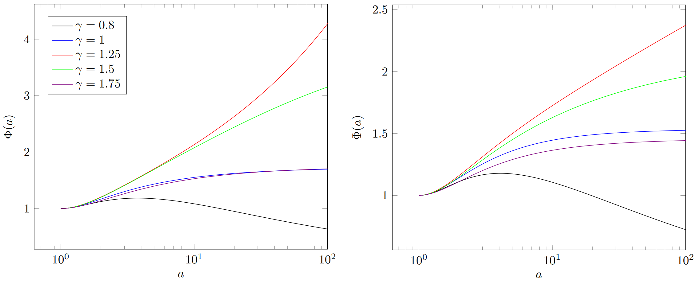
Figure 1: Evolution of perturbations for metric in future as function of scale factor for $\Omega_{de0}=0.72$, $C=0.8$ (left panel), $C=1$ (right panel) for various values of parameter $\gamma$.

where we have dropped the $\cos(kr)/r$ terms, which lead to a singularity at $r=0$. One way to deal with this equation is to take derivative with respect to $t$. This integral equation becomes a differential equation

$$\ddot{\Phi}_{k} +\frac{1}{3H}\Bigg{(}\frac{k^{2}}{a^{2}}+3\dot{H}+3H^{2}+3(4-2\gamma)H^{2}-\frac{3H(5-2\gamma)}{L_{0}}$$ (12)

$$+\frac{4-2\gamma}{2}\frac{a\rho_{de}}{L_{0}}\int_{0}^{l_{h0}(t)}\frac{\sin(kr)}{kr}dr\Bigg{)}\dot{\Phi}_{k}+\frac{1}{3H}\Bigg{(}6\dot{H}H+3(4-2\gamma)H^{3}$$

$$+(2-2\gamma)H\frac{k^{2}}{a^{2}}-\frac{3H^{2}(5-2\gamma)}{L_{0}}-(5-2\gamma)\frac{k^{2}}{a^{2}L_{0}}$$

$$+\frac{4-2\gamma}{2}\frac{\rho_{de}}{kL_{0}}\frac{\sin(kl_{0}(t))}{l_{0}(t)}\Bigg{)}\Phi_{k}=0.$$

This equation for function $\Phi_{k}$ should be solved with equation for $L_{0}$ for the case when $L_{0}$ is the event horizon:

$$\dot{l}_{0}=-\frac{1}{a},\quad l_{0}=\frac{L_{0}}{a},$$

and Friedmann equations

$$\dot{a}=Ha$$

$$\dot{H}=-\frac{1}{2}\left(\rho_{m}+\frac{1}{3}(4-2\gamma)\rho_{de}\left(1-\frac{1}{L_{0}H}\right)\right)$$

Integration of equation for matter density gives a well-known relation

$$\rho_{m}=\frac{D}{a^{3}},$$

where $D$ is integration constant which can be defined from initial conditions. For that purpose, it is convenient to choose initial values of overall density and scale factor

$$a(0)=1,\quad\rho=\rho_{de}+\rho_{m}=1.$$

This choice gives Hubble parameter at $t=0$ value $1/\sqrt{3}$. Equation for $\Phi_{k}$ is invariant under scaling transformation, therefore we can assume that $\Phi_{k}(0)=1$. If $\Phi_{k}>1$ for $t>0$ perturbations grow in future. Currently, $\rho_{de}\approx 0.7$ and $\rho_{m}\approx 0.3$. We estimate $D=0.28$ and find the corresponding initial value of $L_{0}$.

Firstly, we consider perturbations in the case of Tsallis HDE without interaction between matter and dark energy. For brevity we omit index $k$ from $\Phi_{k}$ and consider evolution of mode with $k=0.01$. Our calculations show that dependence of $\Phi_{k}(t)$ on value of $k$ is very negligible. We see the following features (see Fig. 1). For $C=1$ perturbations drop down for $\gamma<1$, but for $\gamma>1$ after some growth function $\Phi$ asymptotically tends to the constant. For $C>1$ the picture is the same. If $C<1$ for some $\gamma$ perturbations increase. Again, as in for $C\geq 1$, for $\gamma<1$ perturbations vanish.

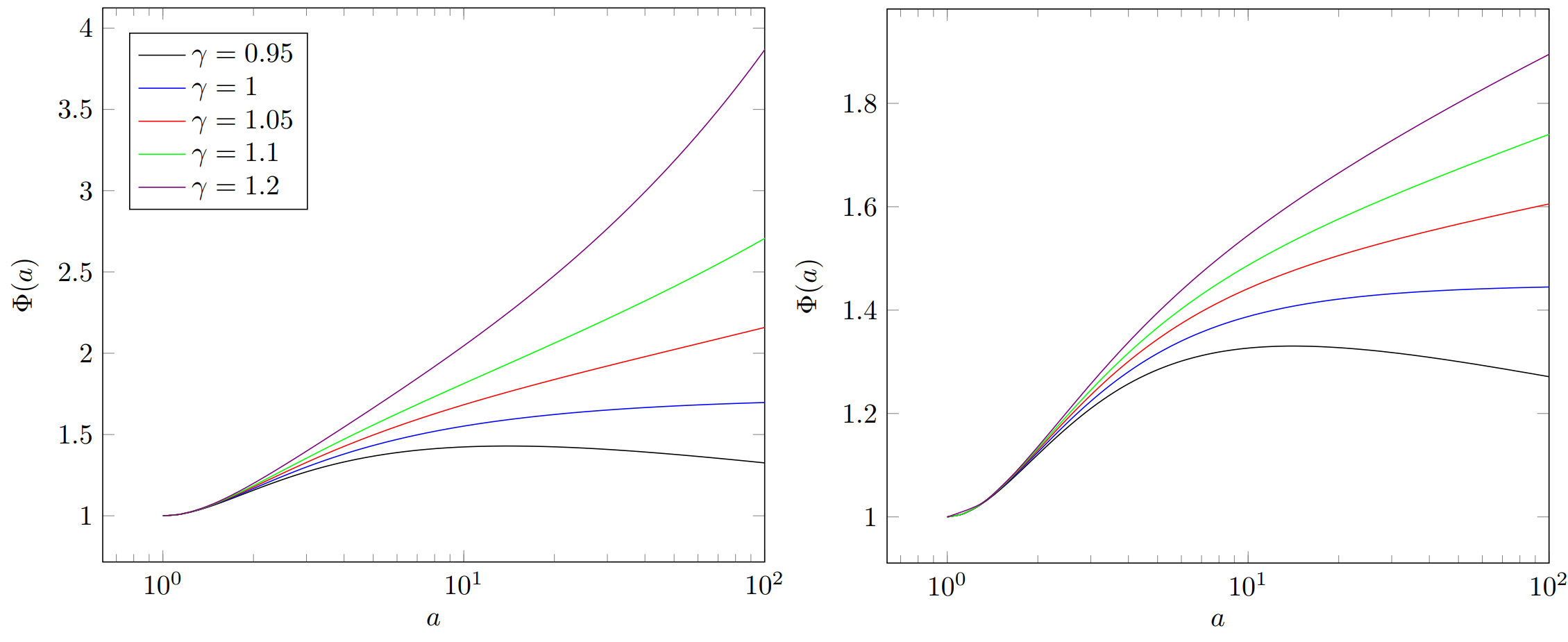
Figure 2: Evolution of perturbations in future with as function of scale factor for $\Omega_{de0}=0.72$, $C=0.8$ (left panel), $C=1.2$ (right panel) for various values of parameter $\gamma$.

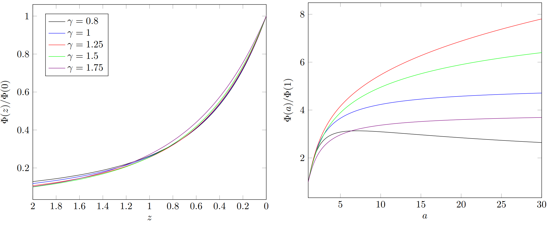
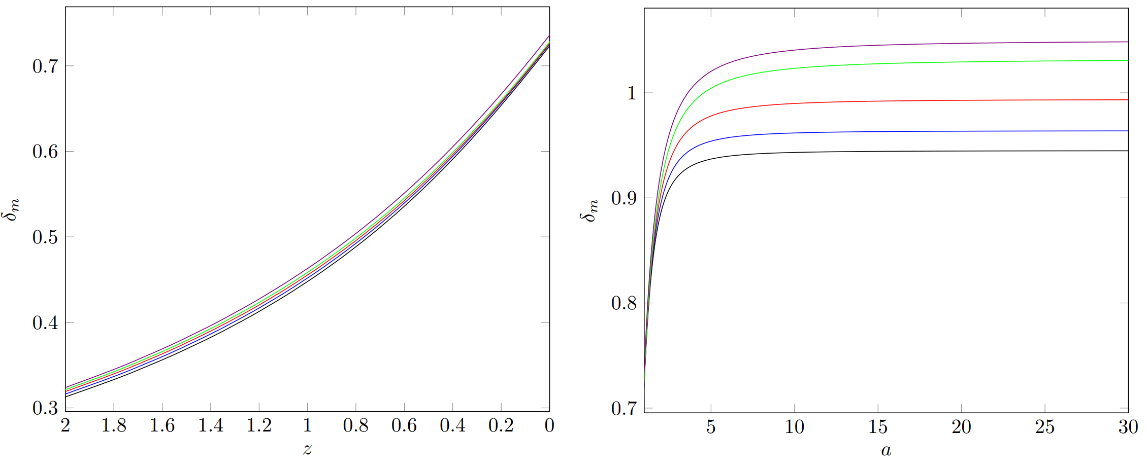
Figure 3: Evolution of metric perturbations in past (upper left panel) as function of redshift $z$ in interval $0<z<2$ and in future as function of scale factor (upper right panel). On down panel the corresponding evolution of matter perturbations is given for past and in future. For current value of $\Omega_{de}$ we take 0.72. Parameter $C=0.8$.

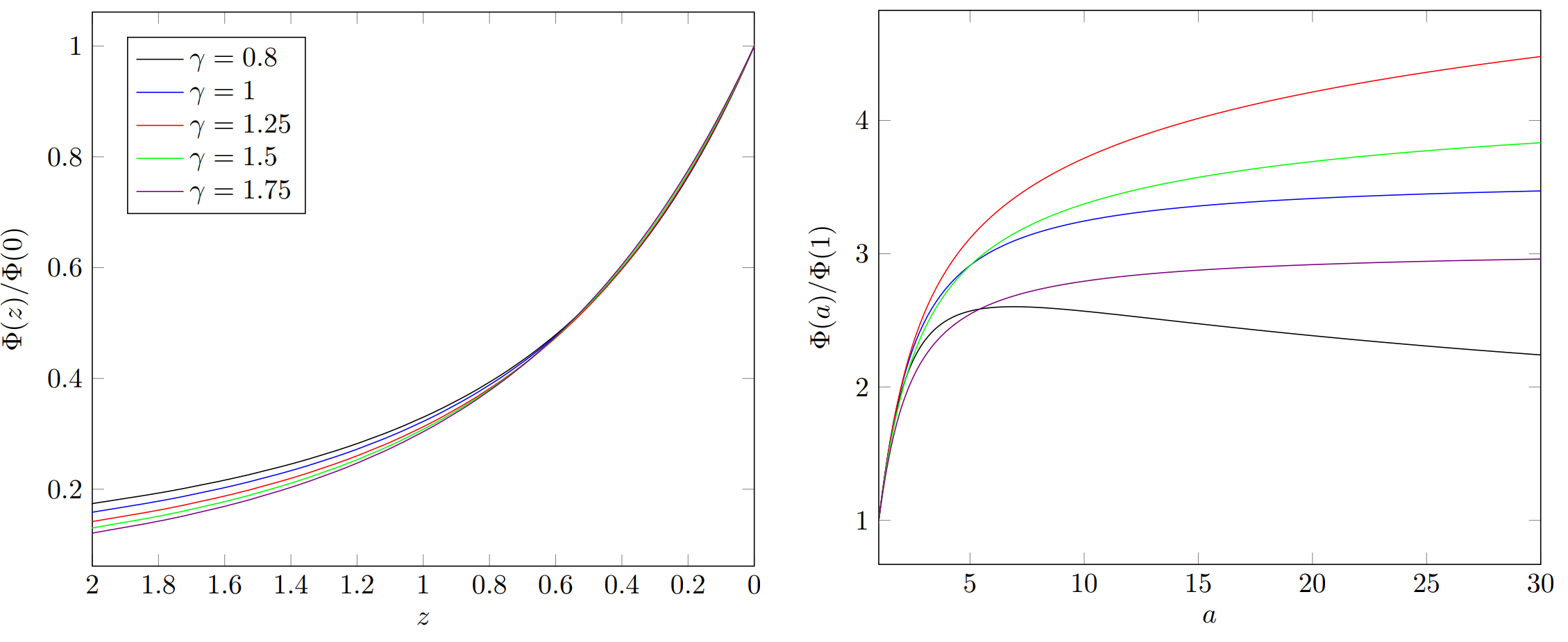
Figure 4: The same as on Fig. 3 but for $C=1$.

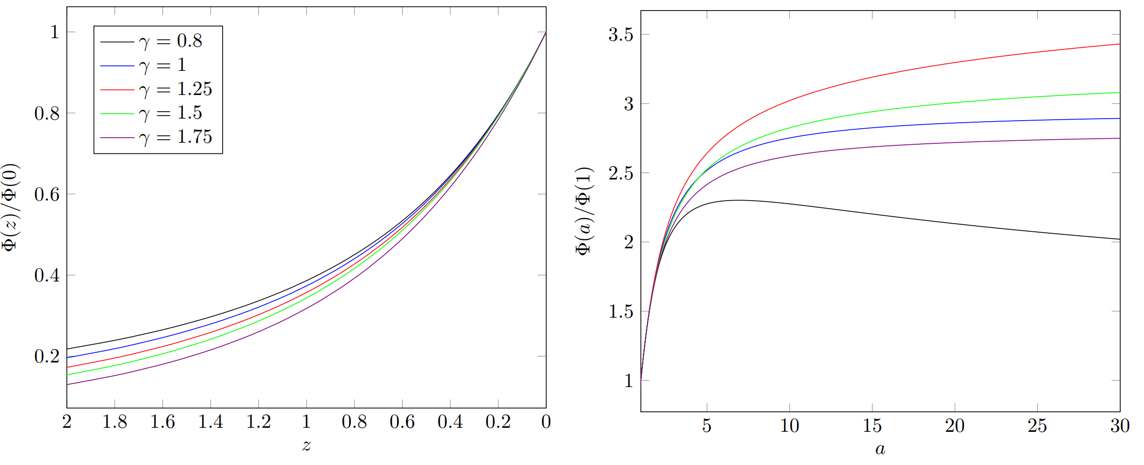
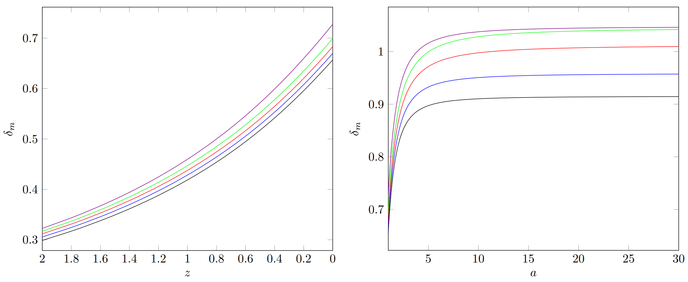
Figure 5: The same as on Fig. 3 but for $C=1.2$.

There is no unambiguous dependence between value of $\gamma$ and growth of perturbations for $C<1$ and $C\geq 1$. From Fig. 1 it can be seen that for $\gamma$ greater than some value the growth rate of perturbations decreases. Numerical calculations allow to conclude that for $1<\gamma<\approx 1.3$ perturbations grow infinitely for $C=0.8$ (see Fig. 2). The critical value of $\gamma$ for $C<1$ depends from $C$.

IV Contribution of matter perturbation

Possible evolution of scalar perturbations deserves to be studied not only at its current state, but in its distant past. Therefore we turn to the early times when $\Omega_{de}<<1$. In this case one needs to account perturbations of matter in r.h.s. of equation (10). The following additional term in equation for $\Phi$ is

$$-\frac{1}{2}\frac{d}{dt}\left(\frac{\delta\rho_{m}}{\rho_{de}a}L_{0}\right)\frac{\rho_{de}a}{L_{0}}=-\frac{1}{2}\delta\dot{\rho}_{m}-\frac{1}{2}\delta\rho_{m}\left((4-2\gamma)H-\frac{5-2\gamma}{L_{0}}\right)$$ (13)

where

$$\delta\dot{\rho}_{m}=\rho_{m}\left(\dot{\delta}_{m}-3H\delta_{m}\right),\quad\delta_{m}=\delta\rho_{m}/\rho_{m}.$$ (14)

Assuming that for relative fluctuation of matter the following representation is valid

$$\delta_{m}(r,t)=\sum_{k}\delta_{mk}(t)\frac{\sin(kr)}{r}$$

we obtain the equation for metric perturbations $\Phi_{k}$

$$\ddot{\Phi}_{k} +\frac{1}{3H}\Bigg{(}\frac{k^{2}}{a^{2}}+3\dot{H}+3H^{2}+3(4-2\gamma)H^{2}-\frac{3H(5-2\gamma)}{L_{0}}$$ (15)

$$+\frac{4-2\gamma}{2}\frac{a\rho_{de}}{L_{0}}\int_{0}^{l_{h0}(t)}\frac{\sin(kr)}{kr}dr\Bigg{)}\dot{\Phi}_{k}+\frac{1}{3H}\Bigg{(}6\dot{H}H$$

$$+3(4-2\gamma)H^{3}+(2-2\gamma)H\frac{k^{2}}{a^{2}}-\frac{3H^{2}(5-2\gamma)}{L_{0}}$$

$$-(5-2\gamma)\frac{k^{2}}{a^{2}L_{0}}+\frac{4-2\gamma}{2}\frac{\rho_{de}}{kL_{0}}\frac{\sin(kl_{0}(t))}{l_{0}(t)}\Bigg{)}\Phi_{k}$$

$$= -\frac{1}{6H}\dot{\delta}_{mk}-\frac{1}{6H}\delta_{mk}\rho_{m}\left((1-2\gamma)H-\frac{5-2\gamma}{L_{0}}\right).$$

For relative fluctuations of matter density we have for sub-horizon scales ($k^{2}>>a^{2}H^{2}$) the following equation for $\delta_{m}$ as function scale factor:

$${\delta}^{\prime\prime}_{m}+A_{m}\delta^{\prime}_{m}=S_{m},$$ (16)

where

$$A_{m}=\frac{3}{2a}\left(1-\delta_{de}\frac{\rho_{de}}{3H^{2}}\right)=\frac{3}{2a}\left(1-\frac{p_{de}}{3H^{2}}\right)$$ (17)

and

$$S_{m}=\frac{3}{2a^{2}}\left(\Omega_{m}\delta_{m}+\left(1+3\frac{dp_{de}}{d\rho_{de}}\right)\Omega_{de}\delta_{de}\right).$$ (18)

The prime denotes the derivative on scale factor. We neglect perturbations of dark energy for matter perturbations assuming that $\delta_{de}=0$ in expressions for $A_{m}$ and $S_{m}$ and therefore

$$A_{m}=\frac{3}{2a},\quad S_{m}=\frac{3}{2a^{2}}\Omega_{m}\delta_{m}.$$

We investigate evolution of matter density and corresponding metric fluctuations from early times when $a_{in}=0.01$. For $\delta_{m}$ we assume that in this moment $\delta_{m}(a_{in})=0.01$ and $\delta^{\prime}_{m}(a_{in})=1$). With account of matter perturbations there is no scale invariance in equation for $\Phi_{k}$. For simplicity we take as initial conditions for $\Phi_{in}$ and $\Phi^{\prime}_{in}$ $10^{-4}$ and $0$ correspondingly. Then we integrate equations from $a=0.01$ to $a=30$ (distant future when $\Omega_{de}\rightarrow 1$). We found $\Phi$ at current value of scalar factor ($a=1$) and consider the relation $\Phi(a)/\Phi(1)$ as function of redshift $z$ in past (in range $0<z<2$) and as function of scale factor in future.

Results of our calculations for various values of $\gamma$ and $C=0.8$, $1.0$, $1.2$ are given on Figs. 3, 4, 5. From our calculations we see that evolution of matter perturbations doesn’t depend significantly from parameter $C$, but value of non-additivity parameter affects considerably on asymptotical value of $\delta_{m}$ on large times. For smaller values of $\gamma$ the limit $\delta_{ms}=\lim_{t\rightarrow\infty}\delta_{m}$ decreases. We see also that evolution of metric perturbations significantly changes in comparison with case when we neglect matter perturbations. There is no significant difference in principal character of evolution of $\Phi$ in past and future only some details change. For all values of $C$ metric fluctuations freeze with time in future but the growth of fluctuations depends strongly from parameter $\gamma$. Also as in a case of neglecting matter perturbations there are no simple correlation between $\gamma$ and asymptotical value of $\Phi(a)$ at large $a$.

V Perturbations in a case of the interaction between dark energy and matter

Let’s consider the model of Tsallis HDE with interaction between dark energy and matter. The interaction between the two components can be introduced by the following. Equations of continuity for components 1 and 2 are

$$\dot{\rho}_{1}+3H(\rho_{1}+p_{1})=0,\quad\dot{\rho}_{2}+3H(\rho_{2}+p_{2})=0,$$ (19)

and are modified as

$$\dot{\rho}_{1}+3H(\rho_{1}+p_{1})=Q_{12},\quad\dot{\rho}_{2}+3H(\rho_{2}+p_{2})=-Q_{12},$$ (20)

where $Q_{12}$ is some function of density of components, time, Hubble parameter, et cetera, in general case. We assume simple possibility for interaction between holographic component of dark energy and matter which are described by the function

$$Q=H({\alpha}\rho_{m}+\beta\rho_{de}).$$

Here $\alpha$, $\beta$, $\lambda$ are some dimensionless constants. For Tsallis HDE we can find pressure using continuity equation with interaction term and obtain the following equation for $\dot{H}$:

$$\dot{H}=-\frac{1}{2}\left(\rho_{m}+\frac{Q}{3H}+\frac{1}{3}(4-2\gamma)\rho_{de}\left(1-\frac{1}{LH}\right)\right).$$ (21)

The pressure of matter is zero and for density of matter one needs to solve the equation:

$$\dot{\rho}_{m}+3H\rho_{m}+Q=0.$$ (22)

Firstly we consider the evolution of metric perturbations without contribution of matter perturbations using Eq. (12) for $\Phi_{k}(t)$. The results for various values of $\alpha$ and $\beta$ are presented on Fig. 6 for $\gamma=1.0$ and $C=1$. For various values of $\gamma$ close to $1$ perturbations decay with time (see Figs. 7 and 8). For some $\alpha$ and $\beta$ solutions with interesting behavior are possible: perturbations initially increase, then decrease and after some increasing they decay finally.

For $C<1$ and $C>1$ function for some $\alpha$ and $\beta$ solutions with interesting behavior are possible: perturbations initially increase, then decrease and after some increasing they decay finally.

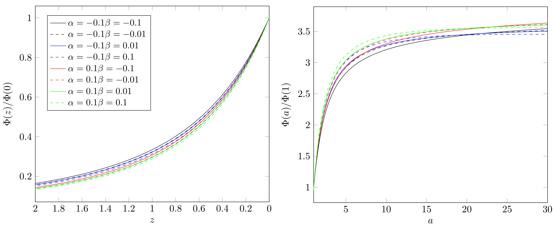
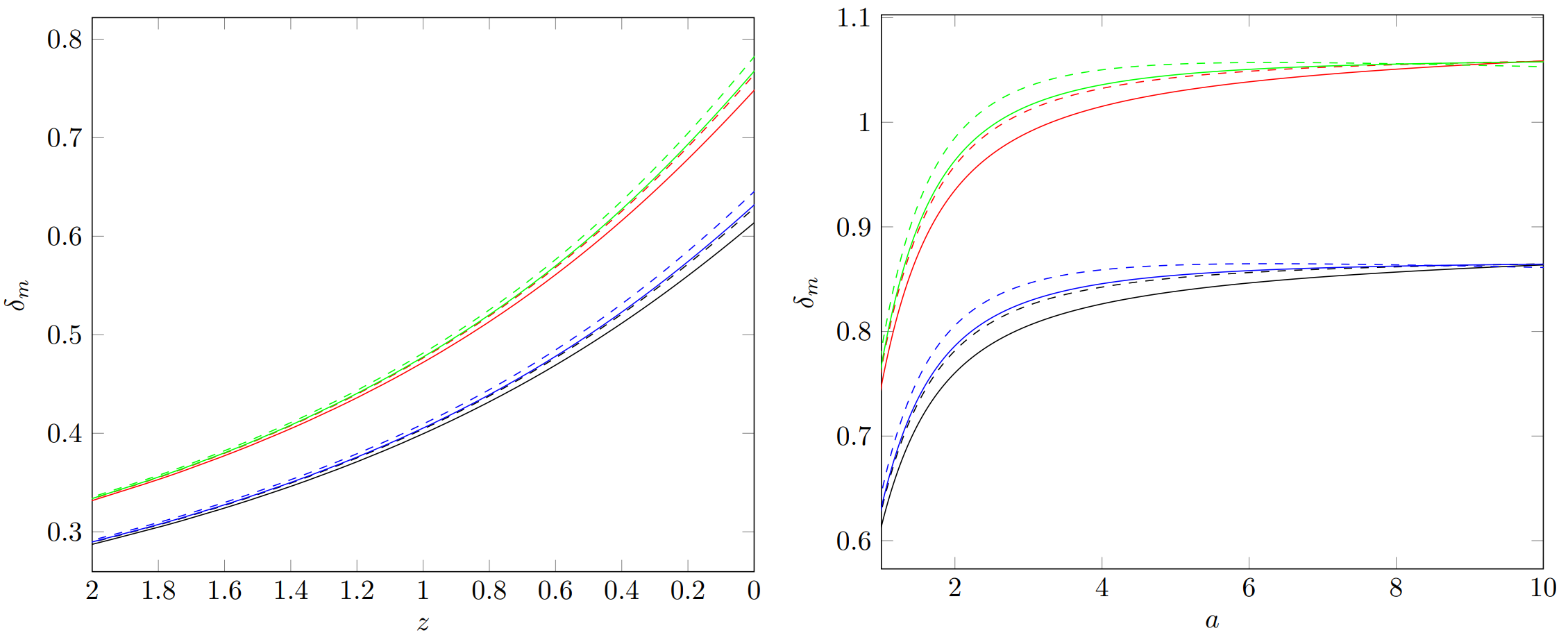
Figure 6: Evolution of metric perturbations in past (upper left panel) as function of redshift and in future as function of scale factor (upper right panel) in a case of interaction between matter and HDE with $Q=H(\alpha\rho_{m}+\beta\rho_{de})$ for various values $\alpha$ and $\beta$. The other parameters are $C=1,\gamma=1$. For current value of $\Omega_{de}$ we take $0.72$. On down panel the corresponding evolution of matter perturbations is depicted. This evolution is sensitive to sign of parameter $\alpha$.

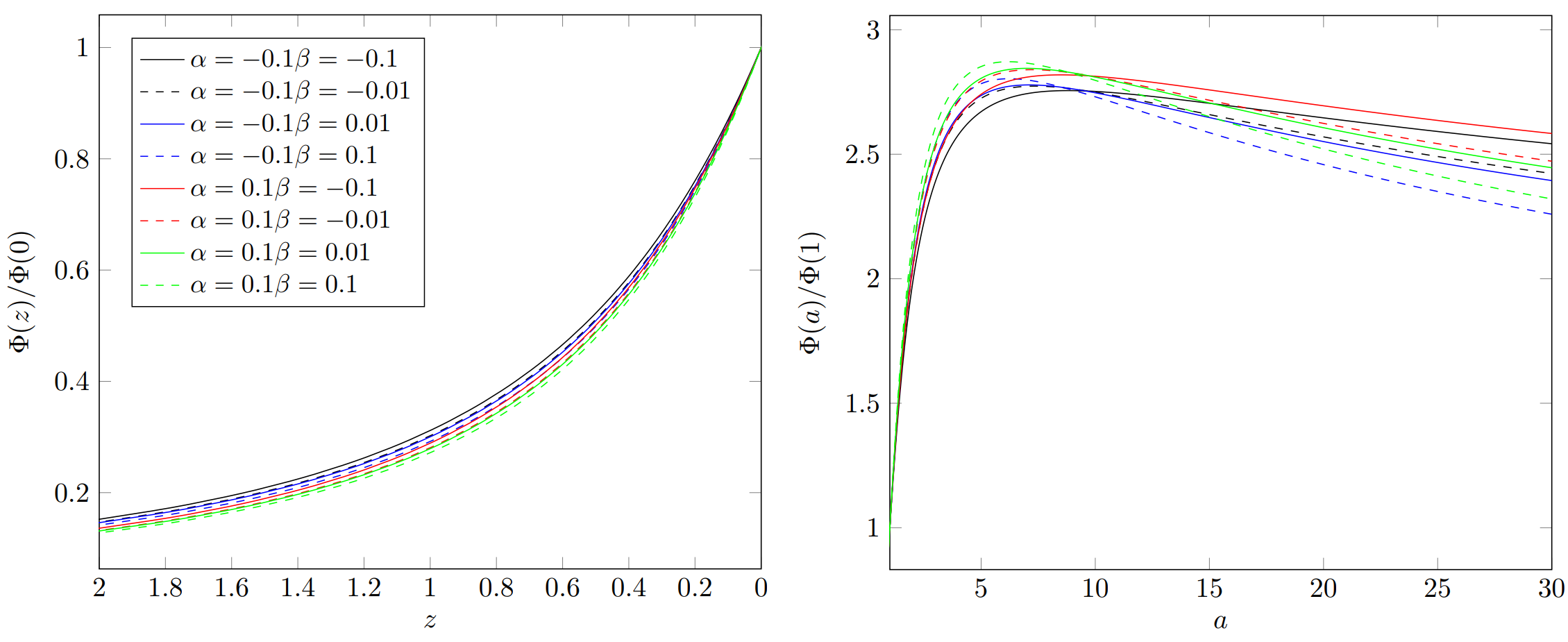
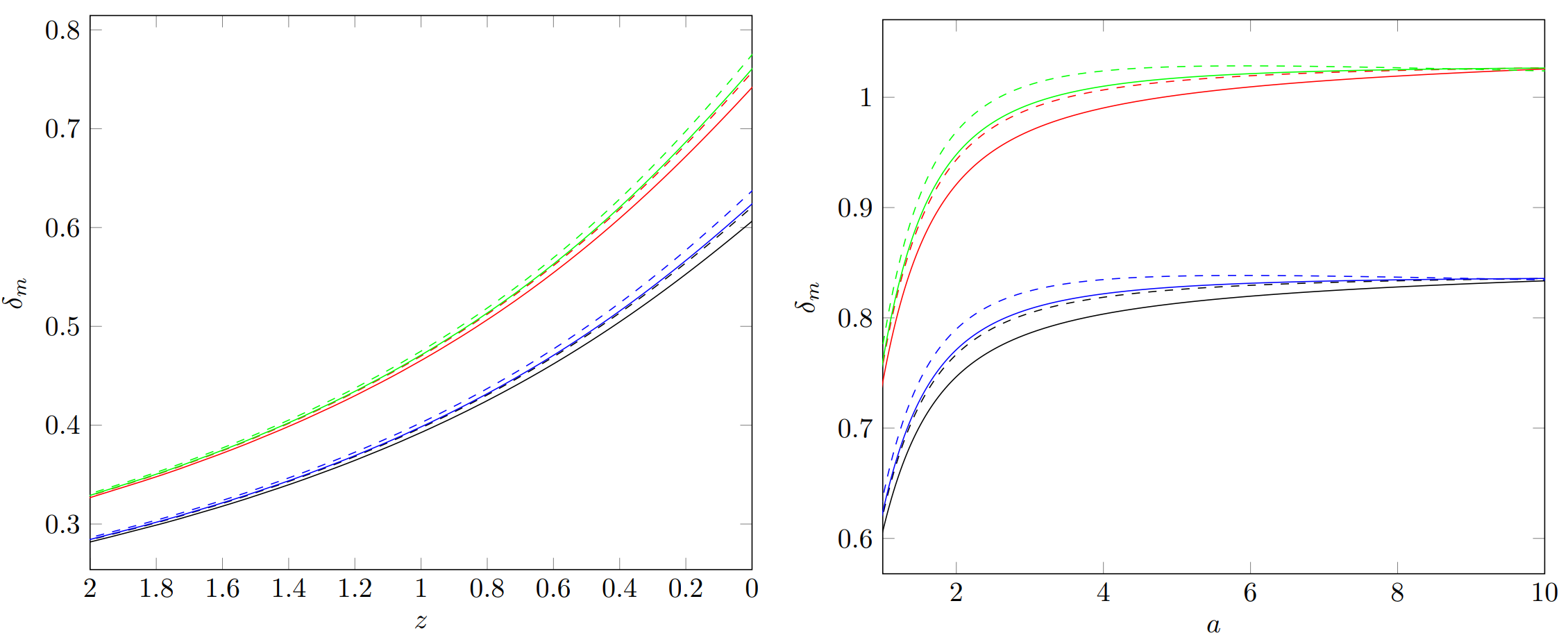
Figure 7: The same as on Fig. 6, but for $C=1,\gamma=0.8$.

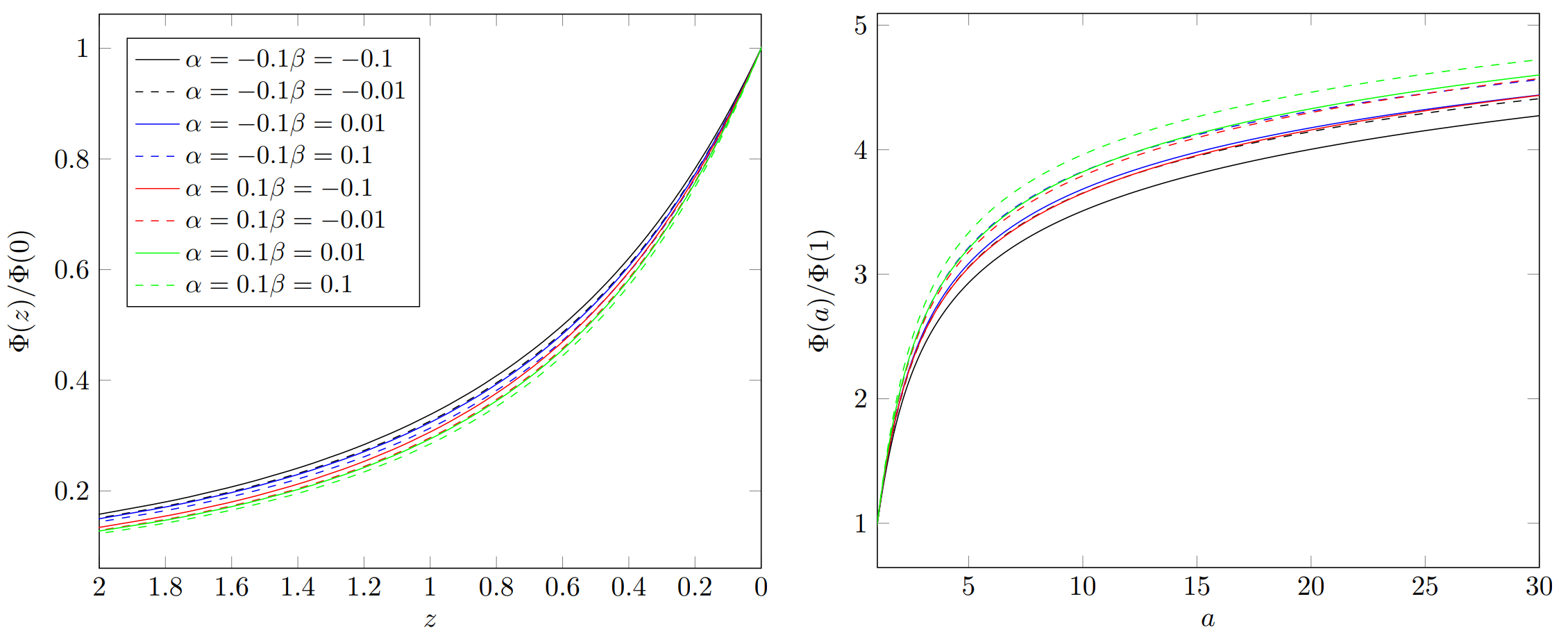
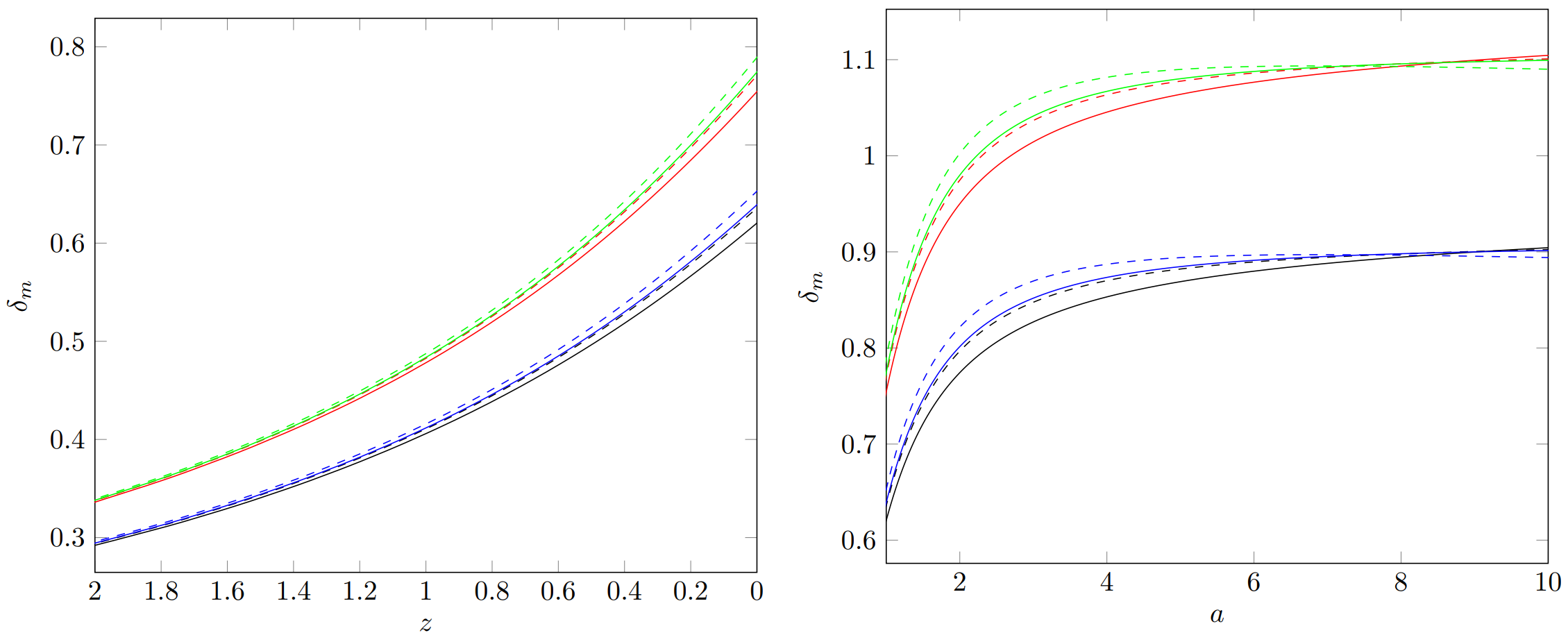
Figure 8: The same as on Fig. 6, but for $C=1,\gamma=1.2$.

If we include matter perturbations in our calculations situation dramatically changes. For metric perturbations we have only numerical but not qualitative difference between cases with different values of $C$ and $\gamma$. The function $\Phi$ asymptotically tends to constant in all cases. The evolution of matter perturbations depends strongly from sign of parameter $\alpha$. For positive $\alpha$ growth of matter perturbations is more than for $\alpha<0$.

VI Evolution of perturbation with inverse Hubble scale as cut-off

Another interesting choice for cut-off is a Hubble horizon. In this case for density of dark energy we have

$$\rho_{de}=3C^{2}H^{4-2\gamma}=3C^{2}\frac{\dot{a}^{4-2\gamma}}{a^{4-2\gamma}}$$

Using relations for $\delta a$ and $\delta\dot{a}$

$$\delta a=-\Phi(r,t)a,\quad\delta\dot{a}=-\dot{\Phi}(r,t)a-\Phi(r,t)\dot{a}$$

one can obtain the following equation for perturbations of dark energy density

$$\delta\rho_{de}=(4-2\gamma)\rho_{de}\left(\Phi(r,t)-\frac{\dot{\Phi}(r,t)}{H}\right){,}$$ (23)

and corresponding equation for modes $\Phi_{k}$:

$$\left(3H^{2}+(\gamma-2)\rho_{de})\right)\dot{\Phi}_{k}+\left(3H^{3}+\frac{k^{2}}{a^{2}}H\right)\Phi_{k}=0.$$

There are two ways of cosmological evolution for such model of holographic dark energy. Firstly, when Hubble parameter approaches to some non-zero constant value. Secondly, scale factor grows and therefore

$$H^{2}\approx\rho_{de}/3=C^{2}H^{4-2\gamma},$$

and for $t\rightarrow\infty$ Hubble parameter

$$H\rightarrow C^{\frac{1}{\gamma-1}}.$$

From equation of perturbations written in form

$$\dot{\Phi}_{k}=-\frac{H+k^{2}a^{-2}H^{-1}/3}{1+(\gamma-2)\frac{\rho_{de}}{3H^{2}}}\Phi_{k}$$

we can conclude that for $\gamma\leq 1$ in the case of HDE-dominated universe perturbation increase infinitely. For $\gamma>1$ $\Phi_{k}$ exponentially decays

$$\Phi_{k}\sim\exp(-\alpha t),\quad\alpha=\frac{C^{\frac{1}{1-\gamma}}}{\gamma-1}.$$

Another case of cosmological evolution corresponds to $H\rightarrow 0$. This is another attractor of system of cosmological equations which is realized when $\gamma<1$. Density of the holographic component also approaches zero and $\rho_{de}/3H^{2}\rightarrow 0$. Universe expansion asymptotically stops and for this scenario perturbations decrease with time.

We depicted the evolution of perturbations and corresponding dependence of Hubble parameter from time on fig. 9.

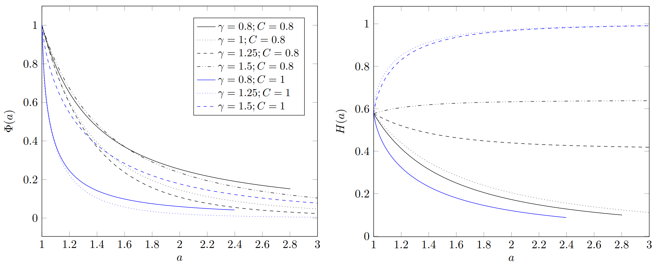
Figure 9: Evolution of perturbations (left panel) and corresponding cosmological dynamics (right panel) for some values of $\gamma$ and $C$. For all considered values of $\gamma$ and $C$ perturbations decay with time.

VII Conclusion

We investigated cosmological model of holographic dark energy in general Tsallis model with $\rho_{de}\sim L^{2\gamma-4}$ with two variants of infrared cut-off $L$, event horizon and inverse Hubble parameter $H^{-1}$. The main question of our paper is the evolution of metric perturbations and matter perturbations for various values of model parameters. In classical approach the criteria for stability is positiveness of square of sound speed which calculates as $dp_{de}/d\rho_{de}$. But holographic dark energy is caused by boundaries of universe and therefore we need to calculate perturbations of horizon using corresponding definition for event horizon or chosen scale cut-off.

In our analysis we considered firstly evolution of perturbations since current moment of time when dark energy dominates, neglecting matter density perturbations. Then we included in our consideration contribution of matter density perturbations and consider evolution from past with very negligible fraction of dark energy. Our investigation shows that account of matter perturbations is very important for metric perturbations. In principle one can say that evolution of metric perturbations defined by mainly by matter perturbations. For wide interval of non-additivity parameter $\gamma$ and $C$ perturbations of metric asymptotically approach constant.

We also investigated possible interaction between holographic component and matter. For interaction $\sim H(\alpha\rho_{m}+\beta\rho_{de})$ with realistic small values of $\alpha$ and $\beta$ freezing of perturbations is faster than it would be for non-interacting dark energy. Even in case of perturbation growth from early times we have its smoothing in future. One note also that evolution of matter perturbations in this case depends from parameters of integration mainly parameter $\alpha$. For negative values of $\alpha$ the asymptotical value of $\delta_{m}$ lies below in comparison with non-interacting case.

If inverse value of Hubble parameter is taken for infrared cut-off, equation for perturbation becomes more simple. Universe filled with Tsallis HDE with this cut-off can approach de Sitter regime on large times when $H\rightarrow\text{const}$. For this we can expect that perturbations will be smoothed out by cosmological expansion but decaying takes place only for $\gamma>1$. For $\gamma<1$ there is a possibility that expansion stops ($H\rightarrow 0$ for $t\rightarrow 0$). Perturbations asymptotically decay for $H\rightarrow 0$. For quasi-de Sitter evolution with $\gamma<1$ perturbations will increase.

Therefore we can conclude that analysis of perturbations for Tsallis HDE based on consideration of HDE as boundary phenomena shows that these cosmological models do not suffer from the problem of perturbations growth.