Random Close Packing of Semi-Flexible Polymers in Two Dimensions: Emergence of Local and Global Order
Abstract
Through extensive Monte Carlo simulations, we systematically study the effect of chain stiffness on the packing ability of linear polymers composed of hard spheres in extremely confined monolayers, corresponding effectively to 2D films. First, we explore the limit of random close packing as a function of the equilibrium bending angle and then quantify the local and global order by the degree of crystallinity and the nematic or tetratic orientational order parameter, respectively. A multi-scale wealth of structural behavior is observed, which is inherently absent in the case of athermal individual monomers and is surprisingly richer than its 3D counterpart under bulk conditions. As a general trend an isotropic to nematic transition is observed at sufficiently high surfaces coverages which is followed by the establishment of the tetratic state, which in turn marks the onset of the random close packing. For chains with right-angle bonds, the incompatibility of the imposed bending angle with the neighbor geometry of the triangular crystal leads to a singular intra- and inter-polymer tiling pattern made of squares and triangles with optimal local filling at high surface concentrations. The present study could serve as a first step towards the design of hard colloidal polymers with tunable structural behavior for 2D applications.
I Introduction
The packing ability and phase behavior of atoms, particles and objects are intimately related to the macroscopic properties of the corresponding physical systems. Packing is thus a key factor in many important physical processes and diverse technological and engineering applications involving for example proteins in living cells, atomic motifs in amorphous and crystal solids, optical photonic and functional materials based on colloidal crystals, stacked piles of cannonballs, oranges in baskets and grains in silos Yuan et al. (2022); Gaines et al. (2016); Conway and Sloane (1999); Manoharan (2015); Börzsönyi et al. (2016); Weaire and Aste (2008); Sheng et al. (2006); Cai et al. (2021); Boles, Engel, and Talapin (2016).
The packing of hard spheres and disks of uniform size in three and two dimensions, respectively, has been extensively studied, advancing our fundamental understanding of the salient features of optimal packing, jamming, crystallization and melting Baranau and Tallarek (2014); Atkinson, Stillinger, and Torquato (2014); Torquato and Stillinger (2001); Lubachevsky and Stillinger (1990); Meyer et al. (2010); Hinrichsen, Feder, and Jossang (1990); Blumenfeld (2021); Jin, Puckett, and Makse (2014); Zaccone (2022); Cheng (2010); Martiniani et al. (2017); Richard et al. (1999); Heitkam, Drenckhan, and Frohlich (2012); Noya and Almarza (2015); Finney (1970); Scott and Kilgour (1969); Conway and Sloane (1998); Bernal and Finney (1967); Medvedev, Bezrukov, and Shtoyan (2004); Luchnikov et al. (2002); Xu, Blawzdziewicz, and O’Hern (2005); Kamien and Liu (2007); Donev, Stillinger, and Torquato (2005); Anikeenko and Medvedev (2007); Torquato, Truskett, and Debenedetti (2000); Desmond and Weeks (2009); Wöhler and Schilling (2022); Gasser (2009); Han et al. (2008); Wojciechowski et al. (2003). In three dimensions, it has been formally proven Hales et al. (2017) that the maximum packing density of non-overlapping spheres, , can be achieved in face centered cubic (FCC) or hexagonal close packed (HCP) crystals and corresponds to .
In practice, in three dimensions, starting from dilute conditions and through compression, the system, be an experimental realization inside a container or a simulation cell subjected to periodic boundary conditions, will reach a jammed state of predominantly amorphous character, where a further increase in concentration is not achievable within the observation time. This state is known as random close packing (RCP) and occurs in a density range that is approximately 10% lower than the maximum achievable one, i.e. . The maximally random jammed (MRJ) state, as introduced in Torquato, Truskett, and Debenedetti (2000), diminishes problems related to the robust definition of the RCP state, as it introduces a more rigorous concept based on volume fraction and the incipient level of order (or equivalently of disorder).
In two dimensions the maximum packing density corresponds to the triangular (TRI) crystal of the wallpaper group, with a corresponding value of surface coverage, . If we consider a triangular monolayer of maximally packed hard spheres, the analogous packing density is approximately . Estimates for the RCP state for disks in two dimensions have been provided by recent theoretical studies Jin, Puckett, and Makse (2014); Zaccone (2022); Blumenfeld (2021), according to which ranges between 0.853 and 0.887.
Independent of whether in experiments or simulations, important challenges must be addressed, first related to the generation of loose, dense, jammed, and maximal hard-body packings and then to the characterization of the resulting systems. The former is a particularly challenging task because of the very high volume fraction associated with jamming and crystallization Ballesta, Duri, and Cipelletti (2008); Donev, Stillinger, and Torquato (2005); Martiniani et al. (2017); Unger, Kertesz, and Wolf (2005); Rissone, Corwin, and Parisi (2021), especially when non-trivial hard shapes are considered Chen, Zhang, and Glotzer (2007); Cinacchi and Torquato (2015); Atkinson, Jiao, and Torquato (2012); Torquato and Jiao (2012); Haji-Akbari et al. (2013); Torquato and Jiao (2009a); Damasceno, Engel, and Glotzer (2012); Anderson et al. (2017). The latter is essential to quantify the degree of disorder among the possible jammed configurations so as to identify the MRJ state Torquato, Truskett, and Debenedetti (2000); Torquato and Stillinger (2010), or the degree of order to gauge crystallization and the corresponding crystal morphologies, or a melting transition Halperin and Nelson (1978); Han et al. (2008); Thorneywork et al. (2017); Bates and Frenkel (2000a); Bernard and Krauth (2011). Efficient simulation algorithms have been developed over the last decades and employed to both create Jodrey and Tory (1981); Tobochnik and Chapin (1988); Torquato and Jiao (2010); Donev et al. (2004a); Jullien et al. (1996); Donev et al. (2004b) and characterize Smith et al. (2008); Richard et al. (1999); Rissone, Corwin, and Parisi (2021); Finney (1970); Donev, Torquato, and Stillinger (2005); Anikeenko and Medvedev (2007); Anikeenko et al. (2007); Hopkins, Stillinger, and Torquato (2009); Kumar and Kumaran (2006, 2005) hard-body packings under a wide variety of conditions.
The complexity in studying packing problems is further augmented when polymer systems are considered, where hard monomers are bonded to form long linear or non-linear sequences. This is due to numerous reasons: first, in contrast to many-particle regular objects like polygons Anderson et al. (2017); Atkinson, Jiao, and Torquato (2012); Wojciechowski, Tretiakov, and Kowalik (2003); Schilling et al. (2005); Marcone et al. (2023); Hou et al. (2019) or polyhedra Torquato and Jiao (2009b); Klement et al. (2021); Jiao and Torquato (2011); Tasios, Gantapara, and Dijkstra (2014); Irrgang et al. (2017); Smith, Alam, and Fisher (2010); Marrucci and Ianniruberto (2004); Torquato and Jiao (2009a), the contour of polymer chains constantly changes so that their shape and size require a statistical description Rubinstein and Colby (2003); deGennes (1980); Doi and Edwards (1988); Kroger (2004); second, additional constraints and parameters in the form of bond lengths, and bending and torsion angles dictate their behavior including the effect of chain length and stiffness, among others; third, due to the wide spectrum of characteristic time and lengths scales Doi and Edwards (1988); Kroger (2004), special techniques Kroger (2019); Weismantel et al. (2022), such as advanced Monte Carlo (MC) algorithms Karayiannis, Mavrantzas, and Theodorou (2002); Theodorou (2010); Kampmann et al. (2021); Kampmann, Boltz, and Kierfeld (2015), are required not only to generate the corresponding polymer packings but to correctly sample the local and global structure of the chains.
In the past we have studied through extensive MC simulations the effect of chain connectivity on the structure Karayiannis and Laso (2008a); Karayiannis, Foteinopoulou, and Laso (2009a); Foteinopoulou et al. (2008), packing ability Karayiannis and Laso (2008a); Laso et al. (2009), phase behavior Karayiannis, Foteinopoulou, and Laso (2009b); Karayiannis et al. (2010); Karayiannis, Foteinopoulou, and Laso (2015) and jamming Karayiannis and Laso (2008a) of athermal systems made of polymers in the bulk and under various conditions of confinement Ramos et al. (2021, 2022). In three dimensions it has been demonstrated that linear, freely-jointed chains of tangent hard spheres i) reach the same RCP limit as monomers Karayiannis and Laso (2008a); Laso et al. (2009); ii) crystallize once a critical concentration range is reached, with the melting point being higher than the corresponding one of monomers and strongly dependent on the gaps between bonds Karayiannis, Foteinopoulou, and Laso (2009b, 2015); iii) form crystal polymorphs of mixed HCP and FCC character and eventually reach perfection in the form of a pure, defect-free FCC cystal Herranz et al. (2022), which is has also been shown to be the thermodynamically stable phase Herranz et al. (2023) as in the case of monomers Bolhuis et al. (1997); Bruce, Wilding, and Ackland (1997); de Miguel, Marguta, and del Rio (2007). Through the use of the - simulator-descriptor software Herranz et al. (2021), our studies have been further extended to treat athermal packings of semi-flexible chains so as to identify the short- and long-range order, corresponding to close-packed crystals (at the level of atoms) and nematic phases of mesogens (at the level of chains), respectively Martinez-Fernandez et al. (2023). The formation of nematic mesophases of prolate or oblate mesogens can precede or be synchronous to crystallization, depending on the equilibrium bending angle Martinez-Fernandez et al. (2023).
The long-range orientational order of polymer chains is traditionally quantified by the nematic director, , that defines the preferred direction of alignment of the molecules Onsager (1949). In three dimensions long-range orientation is quantified by the orientational (nematic) order parameter which gauges the degree of inter-chain alignment along the preferred director . The factors that affect the isotropic to nematic transition for semi-flexible polymers in the bulk, solutions and under confinement have been studied in Egorov, Milchev, and Binder (2016a); Milchev et al. (2018); Egorov, Milchev, and Binder (2016b); Roy and Chen (2021); Roy, Luzhbin, and Chen (2018).
In two dimensions, the reduction of dimensionality leads to a more complex behavior of anisotropic hard bodies where long-range orientational order can be absent or unstable and/or higher-order symmetries prevail like in the form of tetratic, sexatic or octatic phases Schlacken, Mogel, and Schiller (1998); Martínez-Ratón, Velasco, and Mederos (2005); Martinez-Raton and Velasco (2023); Martínez-Ratón and Velasco (2021); Geng and Selinger (2009); Mizani, Naghavi, and Varga (2023a). Theoretical predictions on the singular long-range phase behavior in two dimensions have been confirmed and expanded by simulation and experimental findings, further exploring systematically the effect of aspect ratio and local geometry of the particles and coverage and curvature of the surface Frenkel and Eppenga (1985); Bates and Frenkel (2000b, a); Bowick and Giomi (2009); Gantapara, Qi, and Dijkstra (2015); Anderson et al. (2017); Galanis et al. (2006, 2010); Müller et al. (2015); Narayan, Menon, and Ramaswamy (2006); Donev et al. (2006); Khandkar and Barma (2005) and studying hard-body realizations that include, among others, zig-zag Varga et al. (2009), rod Mizani, Naghavi, and Varga (2023b); Bates and Frenkel (2000b), general-shape Hendley, Zhang, and Bevan (2022); Martínez-Ratón, Velasco, and Mederos (2005); Hou et al. (2020) objects, bend-core trimers Griffith and Hoy (2018) and semi-flexible polymers Chen (1993).
In three dimensions, studies on the crystallization of fully flexible athermal polymers have demonstrated that while monomers are orderly positioned in sites corresponding to close packed crystals Karayiannis, Foteinopoulou, and Laso (2009b); Karayiannis et al. (2010); Karayiannis, Foteinopoulou, and Laso (2015), the corresponding chains behave as ideal random walks, with their statistics being practically unaltered between the initial amorphous state, the intermediate crystal polymorphs and the final stable FCC crystal Herranz et al. (2022, 2023).
In extremely confined monolayers whose thickness approaches the monomer diameter, practically corresponding to 2D systems, freely-jointed chains of tangent hard spheres form a crystal of predominantly triangular (TRI) character whose surface coverage, , is very close to the maximum achievable one as demonstrated in Pedrosa et al. (2023). In parallel, simple geometric arguments suggest that packings approaching ever more closely can be achieved by properly tuning the number of monomers in the simulation cell to comply with the geometric condition of the height-to-width ratio of the perfect hexagon Pedrosa et al. (2023). Effectively, the simulated systems correspond to experimental realizations of spheres being confined in two dimensions, in the form of nanoparticle monolayers Bhattacharjee et al. (2023), as for example microgels between two glass coverslips Han et al. (2008), hard colloidal spherical particles in a cell whose thickness is comparable to the particle size Ruzzi, Baglioni, and Piazza (2023), rod-like hard bodies in aluminum/steel cylindrical or cubic containers loaded on magnet shakers Narayan, Menon, and Ramaswamy (2006); Galanis et al. (2006), or superparamagnetic particles in a quartz cuvette Spiteri et al. (2018). Extremely confined polymer thin films have drawn scientific and industrial attention Marx (2003); Inutsuka et al. (2023); Forrest and Dalnoki-Veress (2001); Ediger and Forrest (2014); Bay et al. (2022); Kritikos et al. (2016); Yang et al. (2023); Carr et al. (2012); Li et al. (2021); Liu and Chen (2010) due to their numerous applications especially as high-performance electronics and organic transistors Cho et al. (2008). Experimental realizations of ultra thin films made of polymers have been reported in the literature corresponding to molecularly flat films, 2D platelets, colloidal 2D crystals, and general self-assembled monolayers Onda et al. (1997); Ganda et al. (2017); Choi (2013); Ariga, Nakanishi, and Michinobu (2006); Wolert et al. (2001); Lin et al. (2000); Yoshida et al. (1999).
In the present contribution we analyze the effect of chain stiffness on the ability of polymers to pack in two dimensions, quantifying the established short- and long-range order and comparing the results with those obtained for freely-jointed chains (having unconstrained bend and torsion angles) and monomers (free of any constraints imposed by chain connectivity). Towards this, we generate various polymer systems with different equilibrium bending angles under dilute conditions, which are then compressed to the maximum achievable packing density by means of long constant-volume simulations. In a last step, quantitative descriptors are employed to gauge the local and global structure of the computer-generated, single-layer polymer packings.
II Model and Simulation Methodology
In the present work we adopt the same polymer model as used in Ref. Martinez-Fernandez et al. (2023) in three dimensions. Linear chains consist of hard spheres of uniform size, with the sphere diameter, , being the characteristic length of the system. Successive monomers are tangent within a numerical tolerance of , the ensuing bond gaps being too small to affect the phase behavior of the chains, as analyzed in Karayiannis, Foteinopoulou, and Laso (2015). Bending angles are controlled by a harmonic potential of the form:
| (1) |
where is the energy, is the bending angle formed by a triplet of successive spheres along the chain backbone (see for example the sketch of Fig. 1 in Martinez-Fernandez et al. (2023)), is the equilibrium bending angle and is the harmonic constant. As in the case of semi-flexible chains in three dimensions Martinez-Fernandez et al. (2023) we set rad-2. The following values have been used for : 0, 60, 90, and , the first and the last corresponding to fully extended (rod) and locally compact configurations, respectively. The 0, 60, and equilibrium bending angles are compatible with the geometry imposed by the connectivity of the sites in the TRI crystal while the is not. Results are compared against the ones of freely-jointed (FJ) chains () and of monomers (free of any constraints imposed by chain connectivity) under the same simulation conditions Pedrosa et al. (2023). Torsion angles are allowed to fluctuate freely in the case of three dimensions and are latter forced to adopt co-planar configurations once a monolayer is formed.
All simulated systems consist of 100 chains () with an average length of , measured in number of spheres, for a total of interacting hard spheres. Due to the presence of chain-connectivity-altering moves Pant and Theodorou (1995), chain lengths of individual molecules fluctuate uniformly in the interval . Packing density, , is defined as the volume occupied by all hard spheres, divided by the total volume of simulation cell. In two dimensions, surface coverage, , is defined as the surface occupied by the parallel projection of the spheres on a large face, divided by the area of each of the two large faces. For monolayers, where film thickness is approximately equal to monomer diameter: .
We use the - software suite Herranz et al. (2021) for the generation, equilibration and characterization of the system configurations. The simulation protocol is a combination of the ones adopted in past works on semi-flexible athermal polymer packings in three dimensions Martinez-Fernandez et al. (2023) and fully-flexible ones in two dimensions Pedrosa et al. (2023). First, initial configurations of freely-jointed chains are generated at very dilute conditions () in three dimensions under periodic boundary conditions (PBCs). Then, the bending potential with the appropirate is activated, while one cell dimension is confined by the introduction of parallel flat and impenetrable walls. Extended constant-volume MC simulations are conducted on the resulting polymer configurations. In the continuation, strong attraction, in the form of a square-well potential, is enforced between one confining wall and all monomers, while repulsion of equal strength is applied on the opposite wall and the monomers. Eventually, this leads to the formation of a monolayer whose thickness is equal to the monomer diameter within a numerical tolerance of . Once the monolayer is formed the attractive potential between the wall and the chain monomers is deactivated.
Starting from this single-layer configuration the long dimensions are then isotropically compressed until a surface coverage of is reached. Then, the process is continued with anisotropic shrinkage of the two large edges of the cell until no further compression can be achieved. This stage corresponds to the random close packed limit in two dimensions for a given value of the equilibrium bending angle, . Constant-volume MC simulations are conducted at the maximum achieved packing density and at specific values of surface coverage, which are all common between the different systems: , 0.60, 0.70 and .
The duration of the MC simulations ranges between 8 and 20 , depending on the packing density and the equilibrium bending angle. Frames (system configurations), along with statistics, are recorded every MC steps. The constant-volume, production simulation corresponds to the following MC scheme Herranz et al. (2021); Ramos, Karayiannis, and Laso (2018); Karayiannis and Laso (2008b): i) reptation (10%), ii) end-mer rotation (10%), iii) flip (34.8%), iv) intermolecular reptation (25%), v) simplified end-bridging, sEB (0.1%) and vi) simplified intramolecular end-bridging (0.1%); where numbers in parentheses denote attempt percentages. As described extensively in Karayiannis and Laso (2008b); Herranz et al. (2021), all local MC moves (types i) through iv)) are executed in a configurational bias pattern with the number of trial configurations, depending on the packing density. As a general rule is set to once surface coverage exceeds the threshold . Neither the attempt percentage nor the number of trial configurations per local MC move change with the value of the equilibrium bending angle.
III Descriptors of Local and Global Structure
The main objective of the present work is to study the effect of chain stiffness, by varying the equilibrium bending angle, on the ability of chains to pack as densely as possible in extremely confined thin films, practically corresponding to monolayers. It is thus essential to quantify the degree of local (at the level of atoms) and global (at the level of chains) order of the corresponding packings. The definition of the MRJ state is, for example, intimately related to the incipient degree of structural disorder Torquato, Truskett, and Debenedetti (2000), which can be quantified indirectly by measuring its antithesis, order, manifested through the presence of sites with crystal similarity. Furthermore, the degree of order depends strongly on the protocol used for the generation of the systems in the vicinity of the RCP limit. Thus, refined metrics are required to gauge the local and global structure of the system configurations as the monolayers, made of athermal polymers, generated here.
III.1 Local Order: Characteristic Crystallographic Element Norm
A critical component of the analysis is to calculate, as precisely as possible, the degree of order (or, equivalently, disorder) in the computer-generated packings in two dimensions. Towards this, the similarity of the local structure with respect to specific crystal templates is quantified through the descriptor part of the - software Herranz et al. (2021), which is based on the Characteristic Crystallographic Element (CCE) norm Karayiannis, Foteinopoulou, and Laso (2009c); Ramos et al. (2020). The CCE norm descriptor is built around the fundamental concept that a unique, and thus distinguishing, set of crystallographic elements and actions corresponds to each crystal in two and three dimensions Giacovazzo et al. (2005). Practically the computer-generated local environment of the closest neighbors around an atom or particle, as identified by a Voronoi tessellation, is mapped onto the ideal one corresponding to a perfect reference crystal, , and depending on the corresponding geometric actions a norm, , is calculated (see for example Eq. 2 in Ramos et al. (2020) and related discussion).
Here, the honeycomb (HON), square (SQU), triangular (TRI) crystals and the pentagonal (PEN) local symmetry are used as the reference ideal structures in two dimensions. Their corresponding characteristic actions and elements together with the exact details on the quantification through the CCE norm, as well as its practical implementation, can be found in Ramos et al. (2020). By further employing a threshold value, , if then the site is labelled as -type. Based on this, and given the highly discriminating nature of the CCE norm descriptor Karayiannis, Foteinopoulou, and Laso (2009c); Ramos et al. (2020), an order parameter can be assigned for each reference crystal , (), which practically corresponds to the fraction of sites with similarity divided by . The degree of (crystalline) order, and of (amorphous) disorder, can be calculated as:
| (2) |
where index above runs over all reference crystals in two dimensions (TRI, SQU and HON). The salient features and the exact algorithmic implementation of the CCE norm descriptor for general atomic and particulate systems in three and two dimensions can be found in Refs. Karayiannis, Foteinopoulou, and Laso (2009c); Ramos et al. (2020); Herranz et al. (2021).
III.2 Global Order: Long-range Nematic Order Parameter
In the present work the degree of long-range orientation is quantified by two order parameters Monderkamp et al. (2022): the first one is the nematic order parameter, , being equal to unity, when all chains are perfectly aligned parallel to the director vector , corresponding to the nematic state, as in the case of three dimensions de Gennes and Prost (1993). The second one is the tetratic order parameter, , which is equal to unity when each pair of chains is either mutually parallel or perpendicular Monderkamp et al. (2022).
To calculate the nematic order parameter, , we adopt the formalism of the order tensor, which in the case of oriented molecules in two dimensions, can be written in the form Frenkel and Eppenga (1985):
| (3) |
where, is the unit vector along the largest semiaxis of the inertia ellipsoid of a chain (considering all of its monomers as points of unit mass), is the isotropic second order tensor, and denote average over all chains. For a system of molecules perfectly aligned in one direction (e.g. direction ), leading to a perfectly nematic mesophase we have:
| (4) |
expressed in the coordinate system of its eigenvectors.
To identify the direction of alignment and to quantify the level of global ordering, we compute the order tensor from equation (3) and subsequently we diagonalize the tensor leading to its diagonal form . The resulting eigenvector corresponding to the largest eigenvalue defines the director and the other one, the direction perpendicular to the director. Moreover, by comparing the eigenvalues with the expected ones for the ideal nematic case (Eq. (4)), we calculate the nematic order parameter from:
| (5) |
In the following, the scalar parameter will be used to quantify long-range (global) nematic ordering, with 0 and 1 corresponding to the limits of isotropic and perfectly aligned, nematic ordering, respectively.
Alternatively, the scalar parameter , which is related to the nematic order parameter usually denoted as Frenkel and Eppenga (1985) and calculated by the 2nd order Lengendre polynomial, could be derived directly from tensor , without the need of diagonalizing the tensor.
| (6) |
To calculate the tetratic order parameter, , we adopt the formalism of the fourth order tetratic tensor Geng and Selinger (2009):
| (7) |
where the components of the tensor are given by:
| (8) |
The tetratic order tensor, given in Eq. 7 has major and minor symmetries: . The 4th order tensor components are represented in a 4x4 matrix following the steps of Ref. Geng and Selinger (2009), condensing both pairs of sub-indices , and , () of the tensor to two sub-indices and () according to the scheme:
| (9) |
The matrix is subsequently diagonalized and its eigenvalues are related to the order parameters and according to Geng and Selinger (2009):
| (10) | ||||
As it is shown in Eq. 10, the sum of the eigenvalues of matrix is zero.
The nematic order parameter, is derived from the eigenvalues of the tensor, while the eigenvalues of the matrix are used to obtain the tetratic order parameter, (), either from the third eigenvalue or from the combination of first and fourth eigenvalues: or from . The tetratic order parameter should not be confused with the fourth order nematic order parameter, it is an additional metric to count for the appearance of tetratic phase. As discussed earlier, a nematic order parameter close to unity is strongly indicative of a nematic phase. In fact, the ideal nematic case, where all chains are oriented parallel to the director, corresponds to both . The tetratic order parameter, on its own, is not sufficient to identify a tetratic phase and thus requires the nematic order parameter to be computed. The ideal tetratic phase, where chains show two perpendicular alignments, corresponds to the limit of and . Finally, the isotropic state of random chain alignment corresponds to .
IV Results
IV.1 Packing Ability
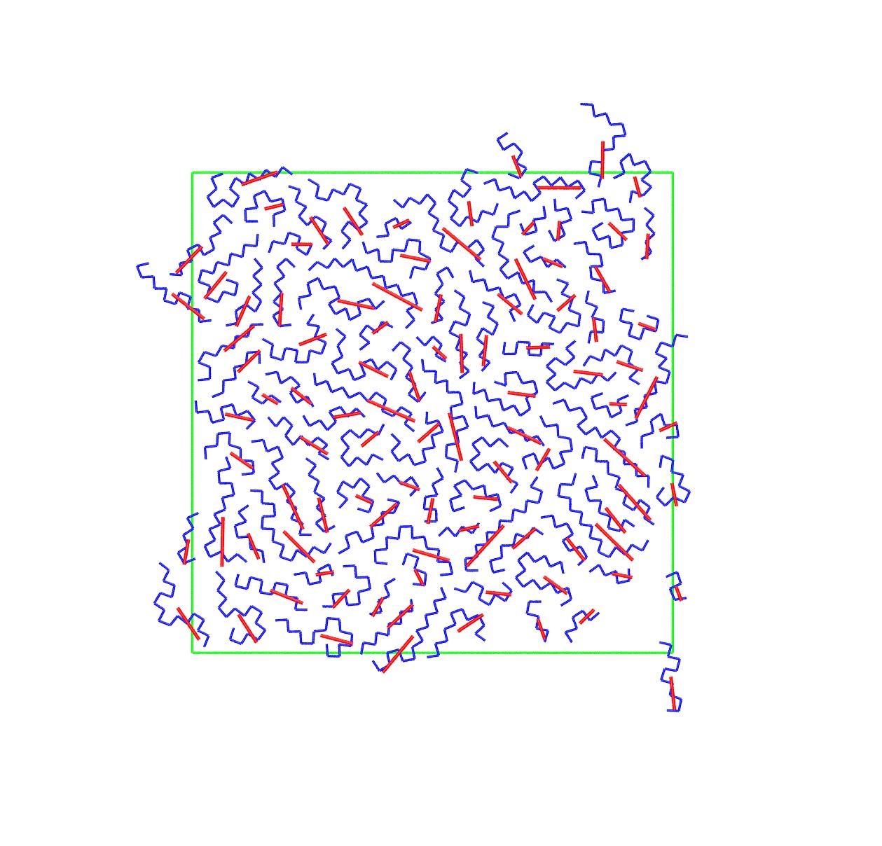
Snapshots at the end of the constant-volume, production MC simulations for all different equilibrium bending angles and at progressively higher surface coverage (packing density) are displayed in Fig. 1, where monomers are colored according to the parent chain and with the coordinates of their centers being subjected to periodic boundary conditions in the two long dimensions of the simulation cell.

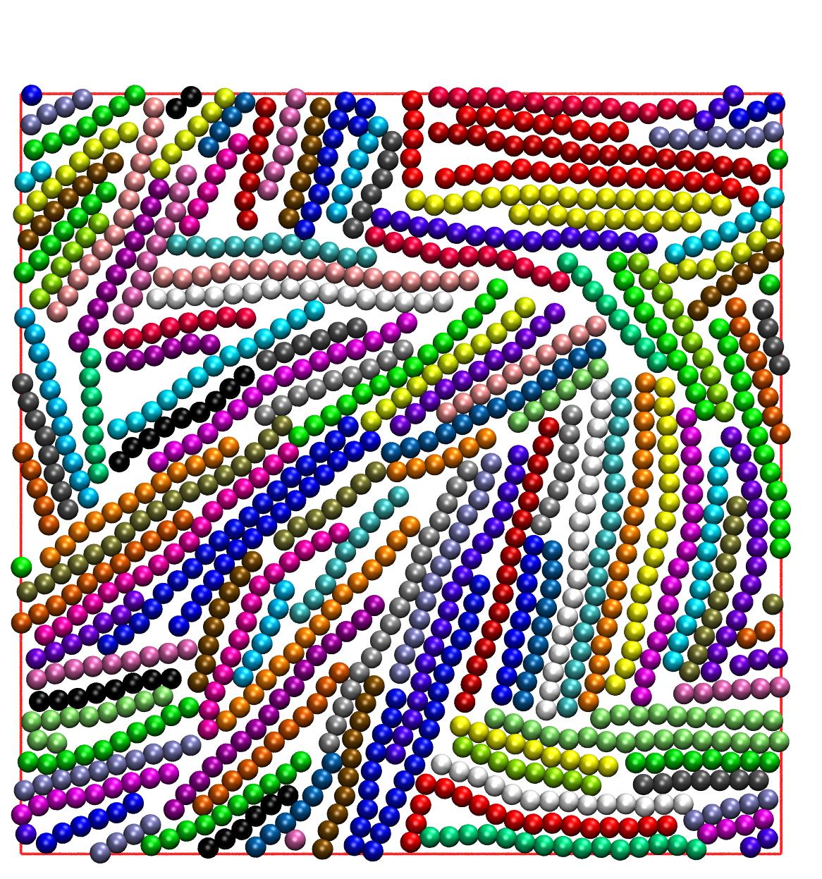
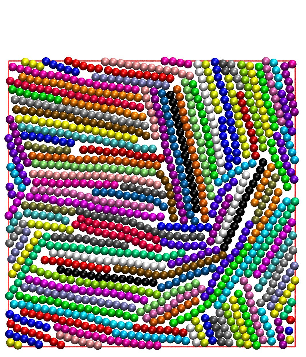
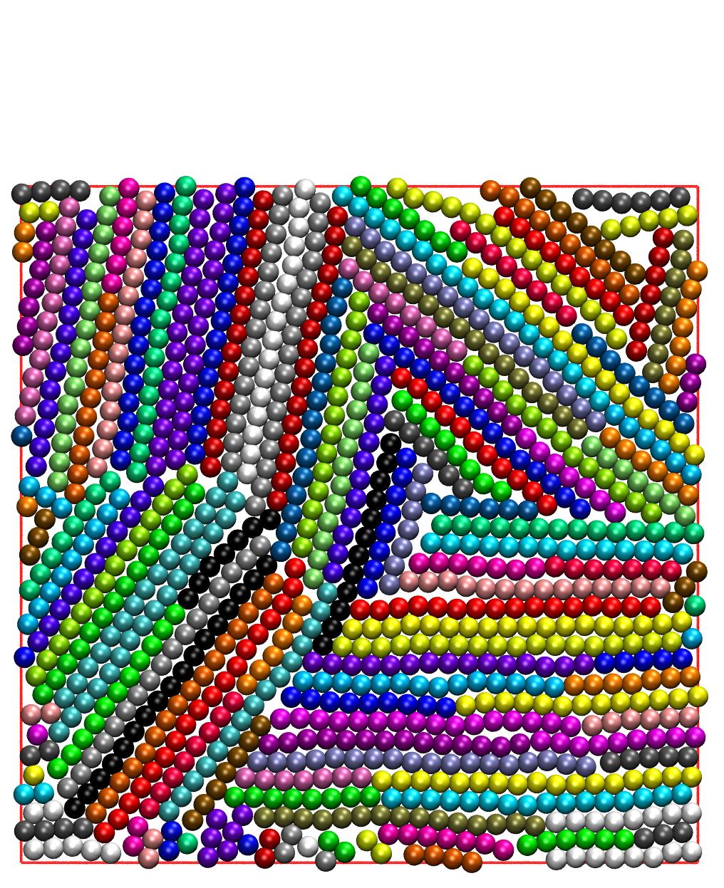
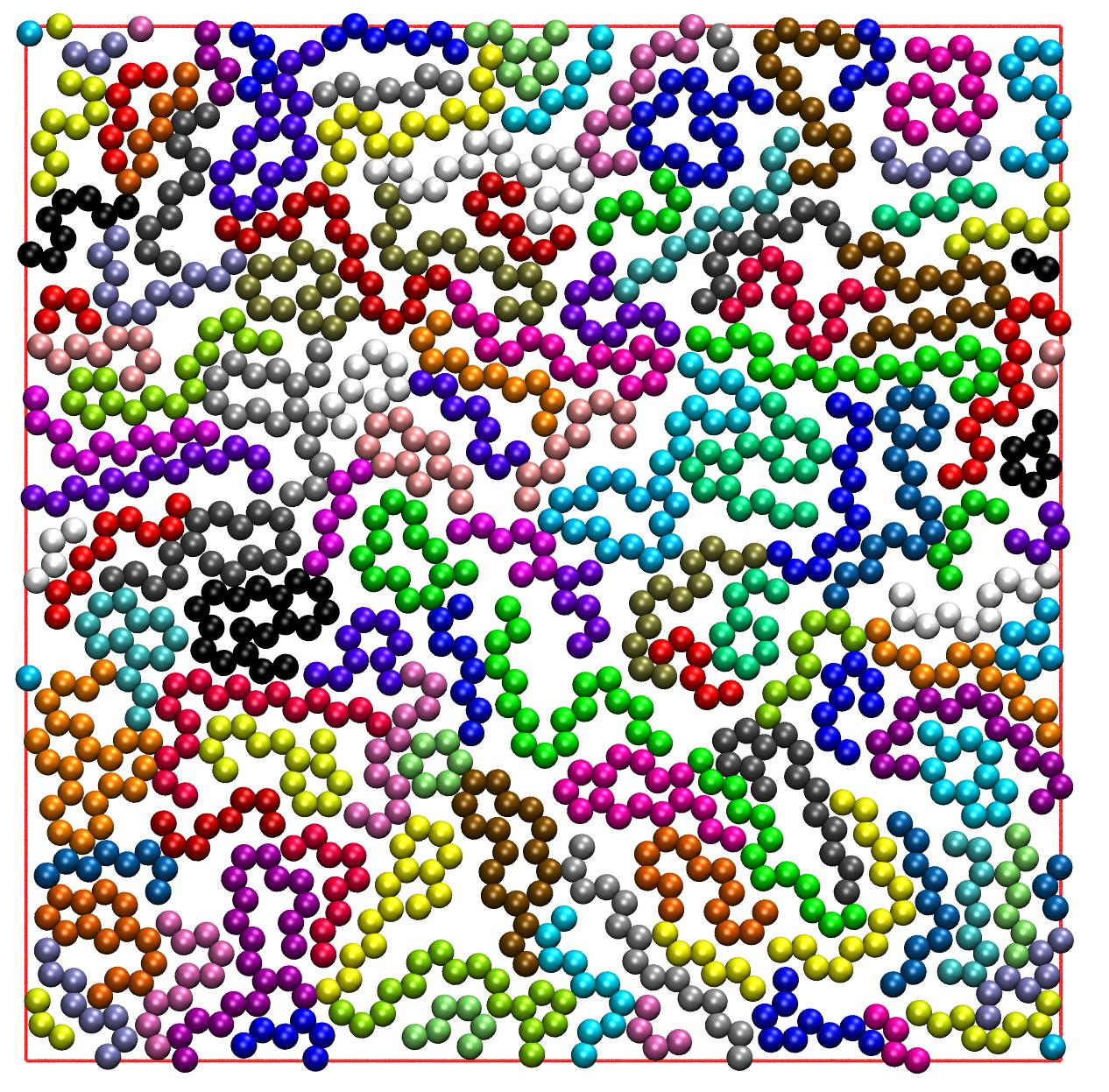
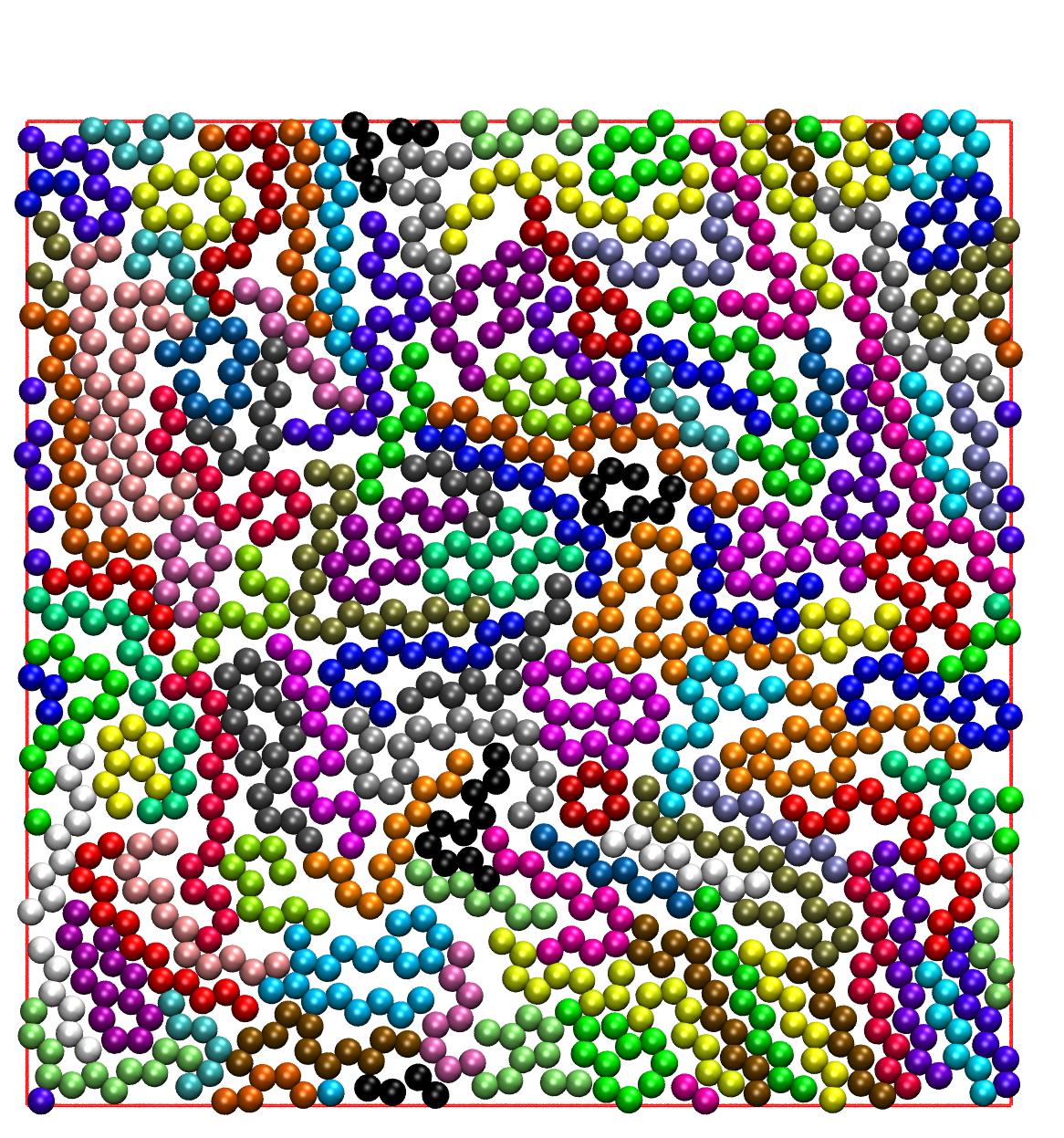


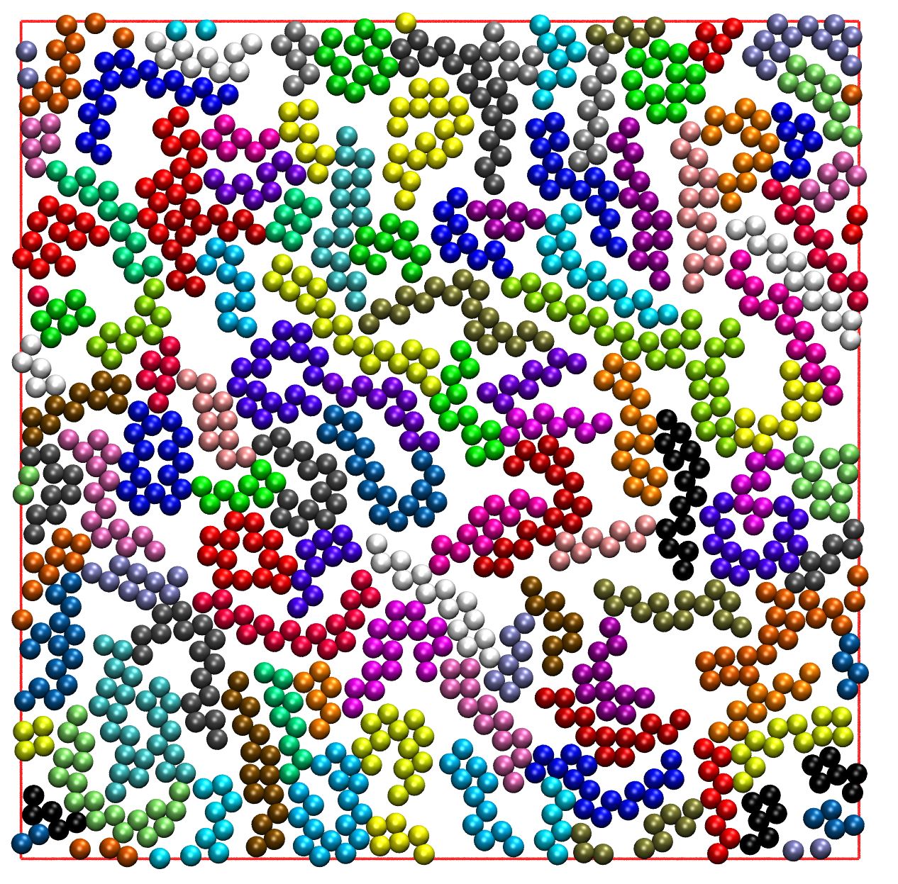

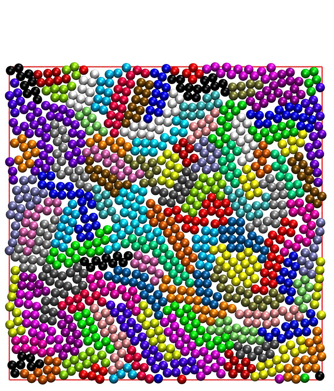

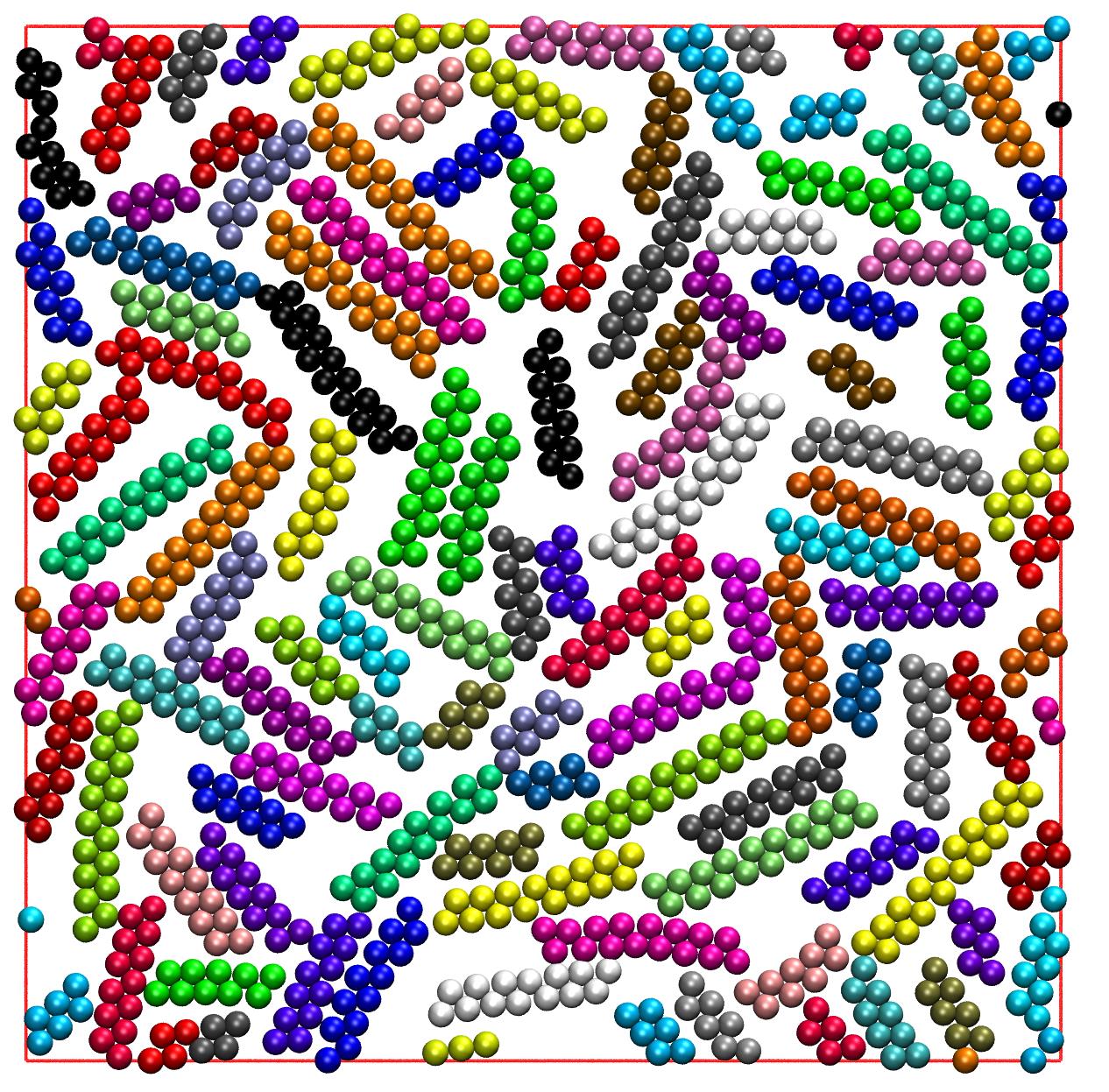
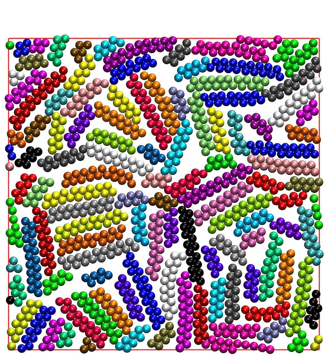
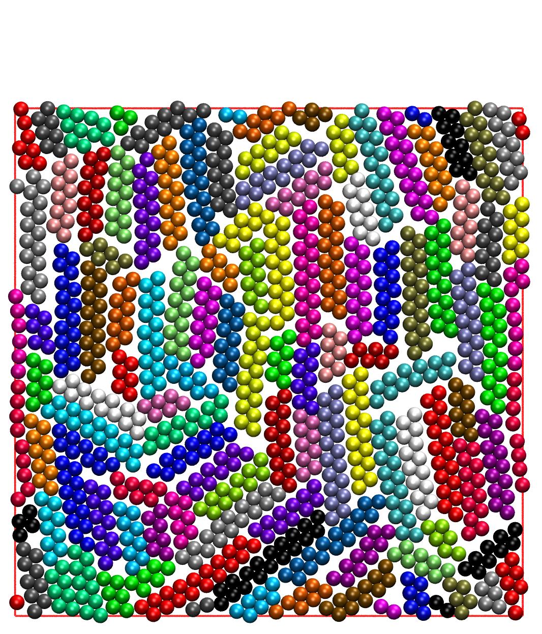
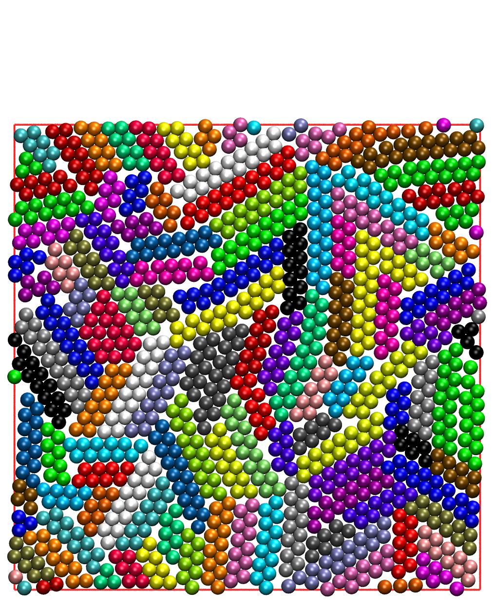
Table 1 summarizes the maximum achievable coverage, , and packing density, , the ratio , average crystallinity, , and long-range nematic and tetratic order parameters, and , corresponding to the RCP limit for a given equilibrium bending angle, , in two dimensions. As a reference the surface coverage for the ideal TRI, SQU and HON crystals is approximately 0.907, 0.785 and 0.604, respectively. The latter is too dilute compared to the surface coverage achieved here over the whole range of equilibrium bending angles so that the HON crystal, even in the form of isolated ordered sites, is very rarely encountered.
From the data on surface coverage the following trend is established: . The fully flexible chains can be packed in the most efficient pattern, whose density lies within 1.4% of the densest limit of the perfect TRI crystal. The least dense RCP limit corresponds to . This is somewhat surprising at first sight given that the is the only angle not encountered between the nearest neighbor sites in the TRI crystal. Given that i) the average chain length studied here is , ii) bonded spheres are tangent and thus by construction also nearest neighbors and iii) chain ends are free of bending constraints, approximately 83.3% of the spheres of the right-angle systems have, at least, two nearest neighbors whose bending conformation is not compatible with the geometry of the TRI crystal.
Thus, this geometric incompatibility for frustrates the formation of the TRI crystal in a similar fashion as the formation of close packed HCP and FCC crystallites in three dimensions can be hindered by bond tangency near the melting point Ni and Dijkstra (2013); Karayiannis, Foteinopoulou, and Laso (2015). Hence, it is expected that the chains cannot achieve surface coverages as high as polymers whose bending angles are geometrically compatible with TRI. In parallel, one should consider that inter-molecular alignment of chains (see discussion on long-range order) further affect the packing ability of semi-flexible polymers. This statement is also relevant in the case of the right-angle chains. The RCP limit of , as calculated from the present MC simulations (), is higher than the surface coverage of the ideal SQU crystal (). Accordingly, the expected sphere arrangement in the monolayer should correspond to a blend of square conformations built through intra-chain arrangements, because of the imposed bending constraints, and more compact local packings achieved through inter-chain conformations. As a consequence in the densest possible state, chains should maximize their external contour (their 2D non-convex hull) available for inter-chain arrangements. In doing so, chains should adopt extended conformations and the higher the concentration the more elongated the corresponding configuration. This is verified by comparing for example the snapshots of the left- and right-most panels in Fig. 1 for . The interplay between inter- and intra-chain arrangements has a major impact in the local and global structure of the chains, as will be demonstrated in the continuation.
| 0.774 | 0.516 | 0.853 | 0.723 | 0.113 | 0.517 | |
| 0.839 | 0.559 | 0.925 | 0.867 | 0.358 | 0.890 | |
| 0.797 | 0.532 | 0.879 | 0.130 | 0.0517 | 0.113 | |
| 0.764 | 0.510 | 0.842 | 0.562 | 0.144 | 0.343 | |
| FJ | 0.895 | 0.597 | 0.987 | 0.945 | 0.396 | 0.187 |
IV.2 Polymer Size
Fig. 2 shows the distribution of bending angles at various surface coverages. The harmonic spring constant of rad-2 allows for the bending angles to thermally fluctuate in an interval of approximately around the equilibrium angle, as in Shakirov and Paul (2018); Shakirov (2019) and in our Martinez-Fernandez et al. (2023) past work on the crystallization of athermal, semi-flexible polymer chains in three dimensions. As shown in Fig. 2, the distribution becomes progressively narrower from to 0.70 for all equilibrium angles except for where the distribution remains practically unaffected by the change in the concentration.

For semi-flexible polymers their size and shape are both dominated by the constraints imposed by chain connectivity and to a lesser degree by packing density. Such constraints are absent in freely-jointed chains and thus their size only depends on volume fraction. Accordingly, for fully flexible athermal polymers four distinct scaling regimes can be identified on the dependence of chain size on volume fraction from dilute to nearly jammed packings Foteinopoulou et al. (2008); Laso et al. (2009). Bond lengths are kept at within a very small numerical tolerance, while the formation of a single layer, whose thickness is equal to the monomer diameter, forces all groups of four consecutive bonds to adopt planar configurations. The distribution of bending angles, which are dominated by the harmonic potential of Eq. 1 has been presented in Fig. 2. This combination of chain geometry, along with surface coverage, leads to a non-trivial effect on polymer size, considering also the different equilibrium bending angles adopted here.
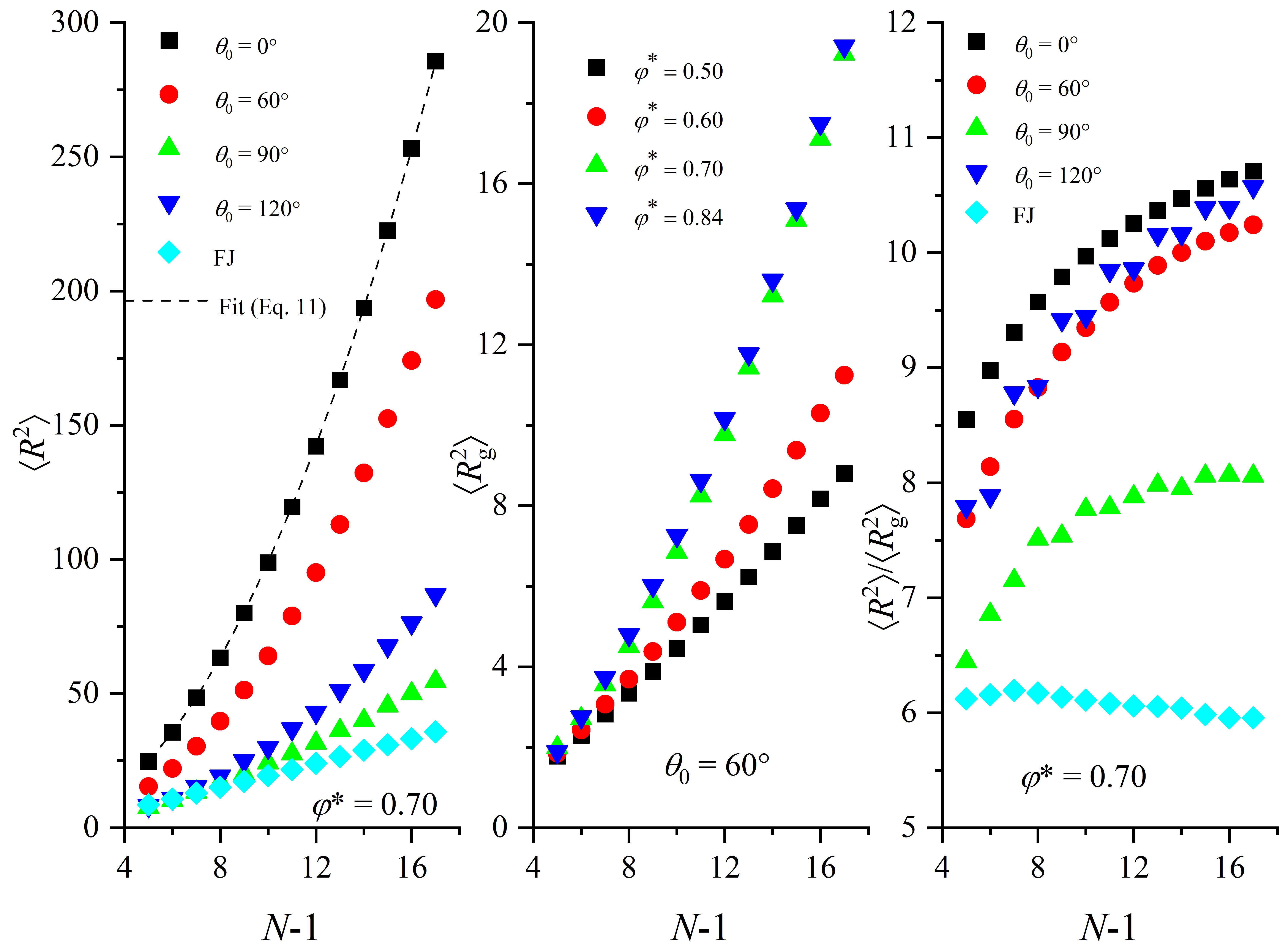
Chain size is quantified through the mean square end-to-end distance, , and the mean square radius of gyration, , where brackets denote averaging over all chains and system configurations. Furthermore, as simulations are conducted on systems with chain length dispersity and because chain-connectivity-altering moves guarantee the robust sampling of the long-range polymer conformations, the effect of chain size on chain length in the range (Fig. 3) can be obtained straight from the MC frames. Left and right panels present the dependence of and of the ratio , respectively, on the number of bonds per chain, , at a surface coverage of for all equilibrium bending angles studied here, including a comparison with the freely-jointed (FJ) chains. Given that the rod-like chains simulated here correspond to very small value of we can fit the simulation data with the analytical predictions of the worm-like chain model Kratky and Porod (1949) according to which Rubinstein and Colby (2003); Hsu, Paul, and Binder (2011):
| (11) |
where is the maximum chain length () and the persistence length. In the rod-like limit (), as in here, we have . Such a fitting is also shown along with the corresponding simulation data () on the left panel of Fig. 3.
The middle panel shows the dependence of on for at various surface coverages. Acute bending angles of and lead to more elongated chains while freely-jointed systems are the most compact. As packing density increases, chain size increases, but there is no appreciable difference in the radius of gyration between and . With respect to the ratio the freely-jointed chain system reaches a plateau value very close to 6, followed by the right-angle system for which . The remaining systems show a systematic increase of the ratio with chain length, suggesting that the simulation of longer chains is required to observe ideal polymeric behavior. For comparison, the limits of fully flexible and very stiff chains in the worm-like (Porod-Kratky) model correspond to and 12, respectively Rubinstein and Colby (2003).
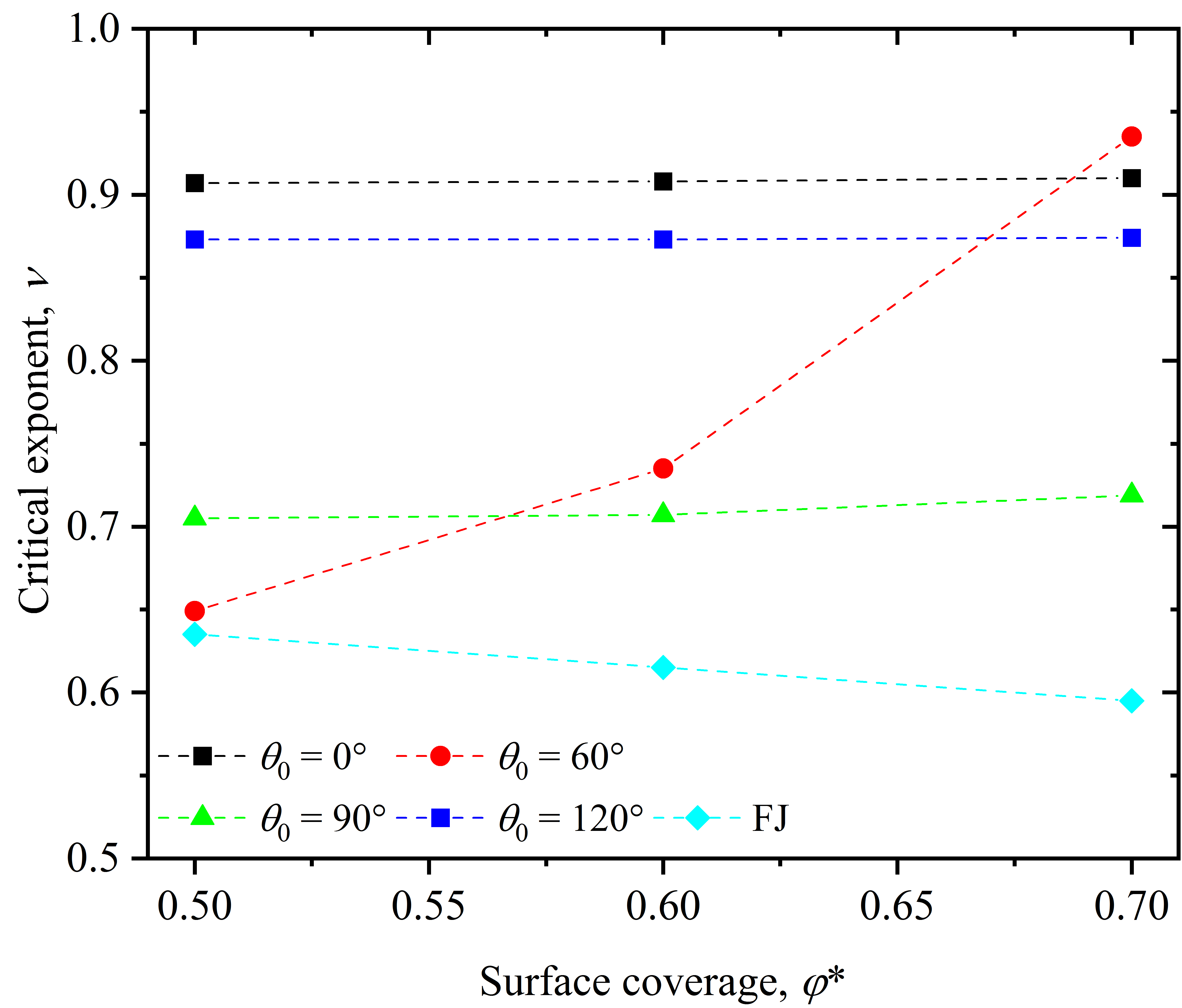
One can also extract the critical Flory exponent, , from the dependence of chain size on chain length, through , considering the number of bonds instead of the number of monomers, given the short chains studied here. In two dimensions and considering excluded volume interactions and chain coiling Flory (1989). The maximum chain extensibility corresponds to an all-trans, rod-like or zig-zag configuration according to which , i.e. . On the other limit the densely packed and fully collapsed polymers correspond to Schluter, Payamyar, and Ottinger (2016). Fig. 4 shows the dependence of on surface coverage for semi-flexible polymers of different equilibrium bending angles, together with a comparison with fully flexible chains under the same conditions. The exponent is calculated from the simulation data of versus , as for example the one presented in the middle panel of Fig. 3. Rod-like systems corresponding to show a Flory exponent which is independent of packing density and approximately equal to 0.91. This value is slightly lower than the expected one for rods (). This small deviation is due to bending angles following a distribution around the equilibrium value, as seen in Fig. 2, rather than all being exactly equal to . The locally compact system of shows also high value of the critical exponent, which is again unaffected by packing density. Chains with are characterized by significantly lower values of , which do not depend on surface coverage. In contrast, the scaling exponent for the fully flexible chains shows a decrease as packing density increases as a result of the progressive chain collapse. In parallel, the most profound effect of surface coverage is encountered for as increases markedly until it reaches a value of at . This trend, as will be demonstrated in the continuation, is strongly related to the formation of a nematic phase where chains adopt maximum length, zig-zag conformations.
Focusing on rod-like systems Ref. Bates and Frenkel (2000b) has demonstrated that spherocylinders confined to a plane show a nematic phase when their aspect ratio is higher than a threshold value, , where is the length and the diameter (the limit of corresponding to needles Frenkel and Eppenga (1985)). Shorter rods show an isotropic phase where chains are aligned either side-by-side or perpendicular to each other Bates and Frenkel (2000b). In our rod-like case () we have dispersity in chain lengths combined with a distribution of bending angles around the equilibrium value resulting in a shape which is not fixed but rather changes continually over the simulation. Thus, our computer-generated samples deviate from the ideal, fixed-shape hard rods of the aforementioned studies. Still, we can attempt a comparison of the aspect ratio as a function of surface coverage and by considering that and . For , and at all surface coverages studied here, including the one of the RCP limit, approximately 23% of the chain population, corresponding to lengths = 6, 7 and 8, have aspect ratio . This could potentially make the observed nematic phase, if such phase exists in our simulations, unstable compared to systems of significantly longer chains. The analysis in Ref. Mizani, Naghavi, and Varga (2023a) for infinitely thin rods (needles) demonstrates that rod length dispersity affects significantly the phase behavior, with long and short rods stabilizing and weakening, respectively, the nematic phase.
IV.3 Local Structure: Crystallinity
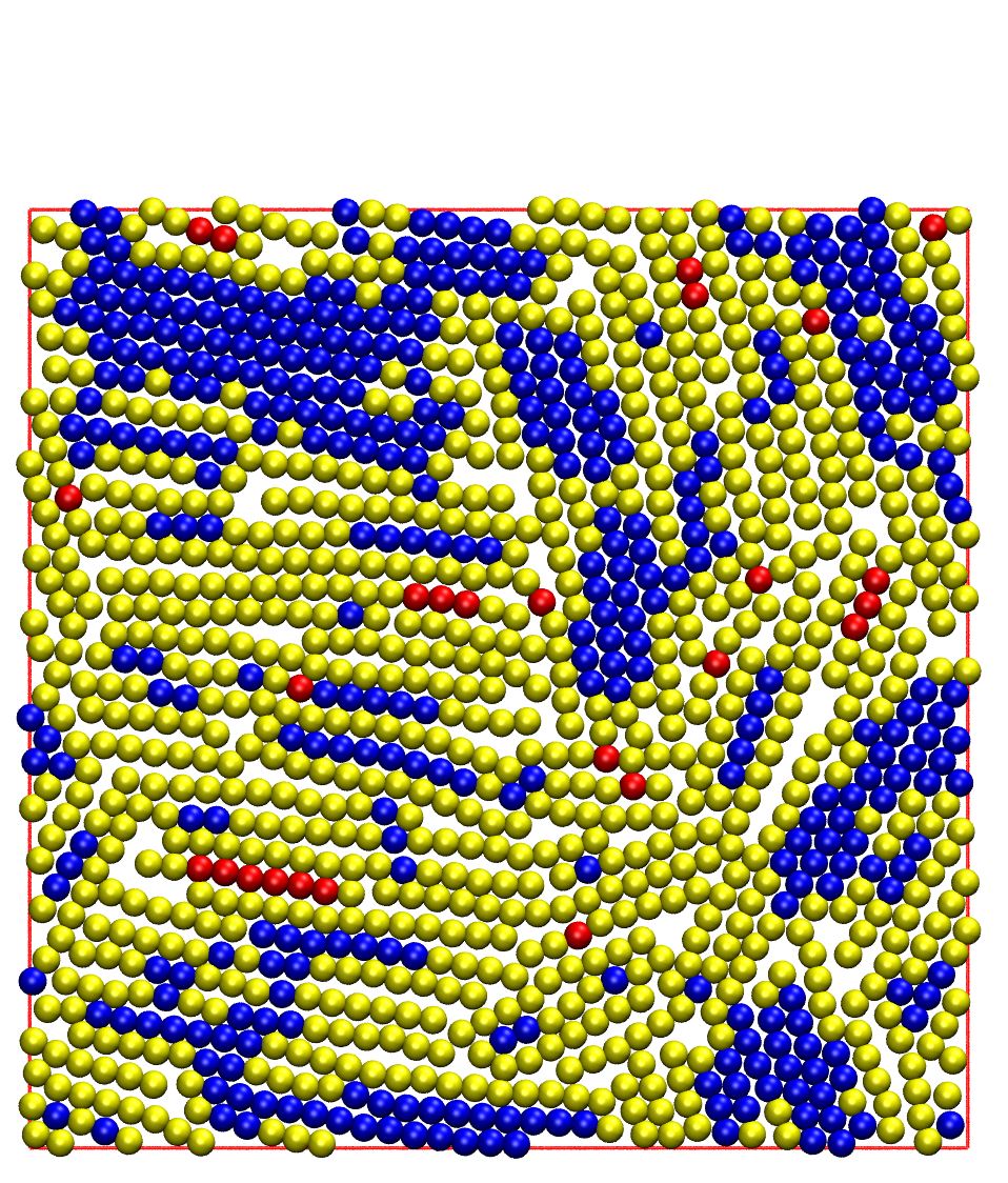
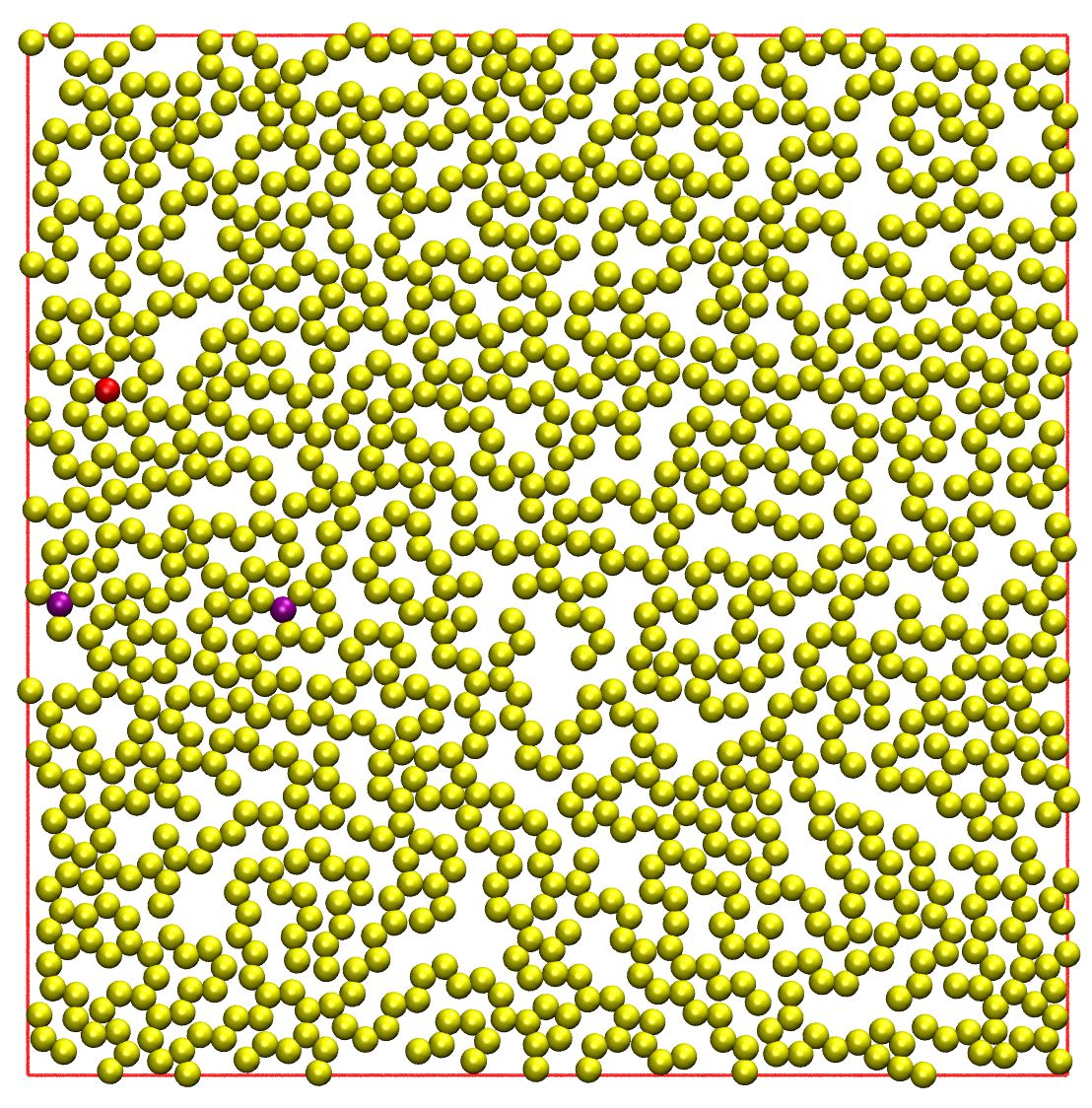
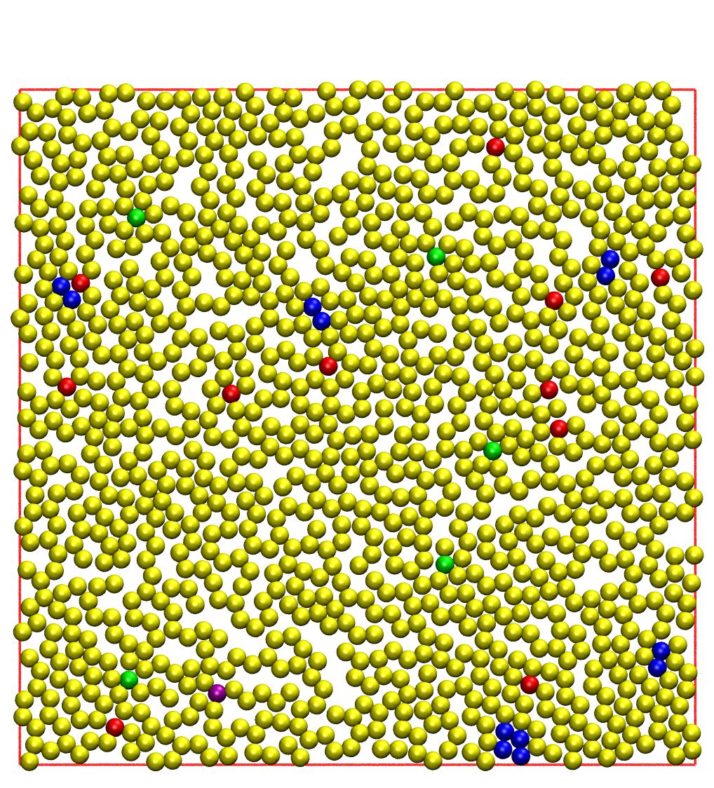
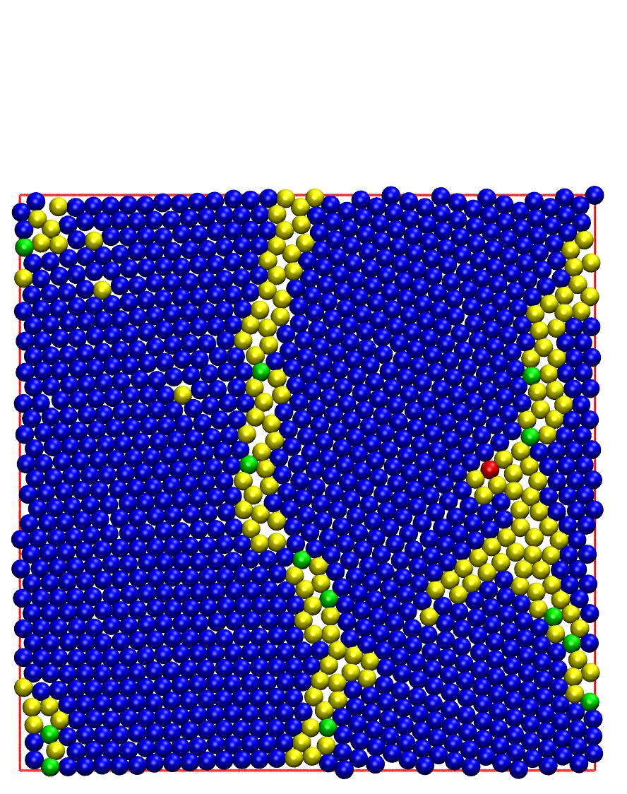
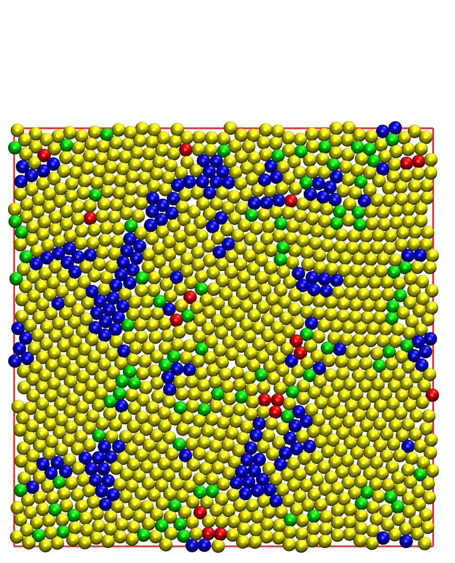
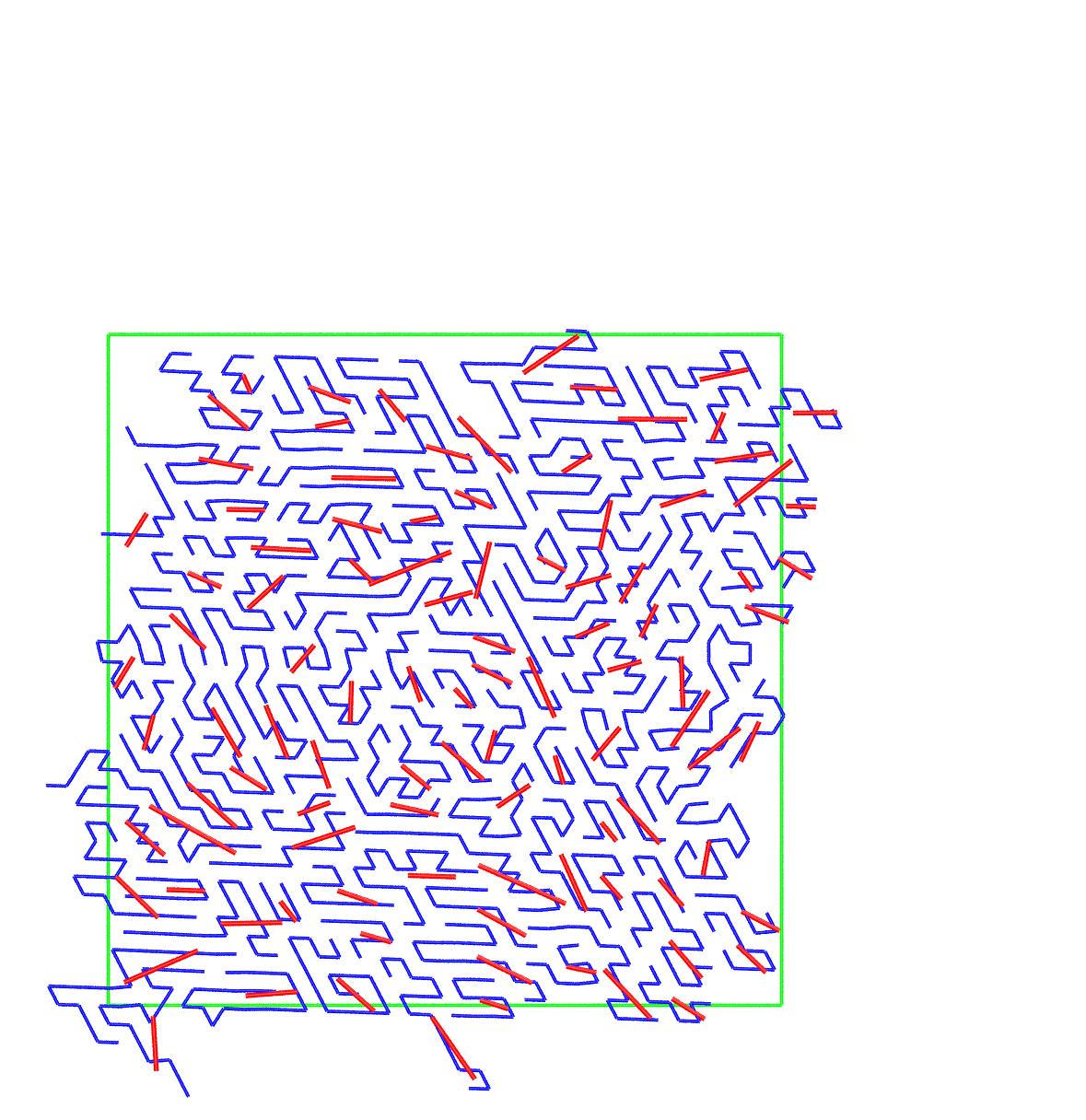
One essential element in the identification of the crystal phase, MRJ state or RCP limit is the quantification of local order. Here we employ the CCE norm descriptor Ramos et al. (2020) to quantify the structural similarity of the local environment around each monomer against the triangular (TRI), square (SQU) and honeycomb (HON) crystals and the pentagonal (PEN) local symmetry in two dimensions. In all calculations to be presented below a threshold of is adopted. Spheres with TRI, SQU, HON and PEN similarity are colored in blue, red, purple and green, respectively. Monomers whose CCE norm is higher than the threshold value for all reference crystals and local symmetry are labeled as amorphous (AMO), or more precisely as "unidentified", and are shown in yellow.
Fig. 5 shows system snapshots at the end of the MC simulations at different packing densities, including the densest ones for each equilibrium bending angle. Monomers are colored according to the CCE norm description as explained in the previous paragraph. At the lowest surface coverage () all systems are predominantly amorphous and the number of sites with crystal structure is very low. As density increases crystallinity increases and the ordered sites form small, isolated clusters. These clusters grow in size as concentration increases, as can be observed at . Finally, at RCP all systems exhibit the highest local order. Given the very high values of surface coverage the RCP limit for , 60, 90 and corresponds to a TRI crystal, ridden with defects in the form of amorphous sites and free of isolated clusters of other crystal morphologies.
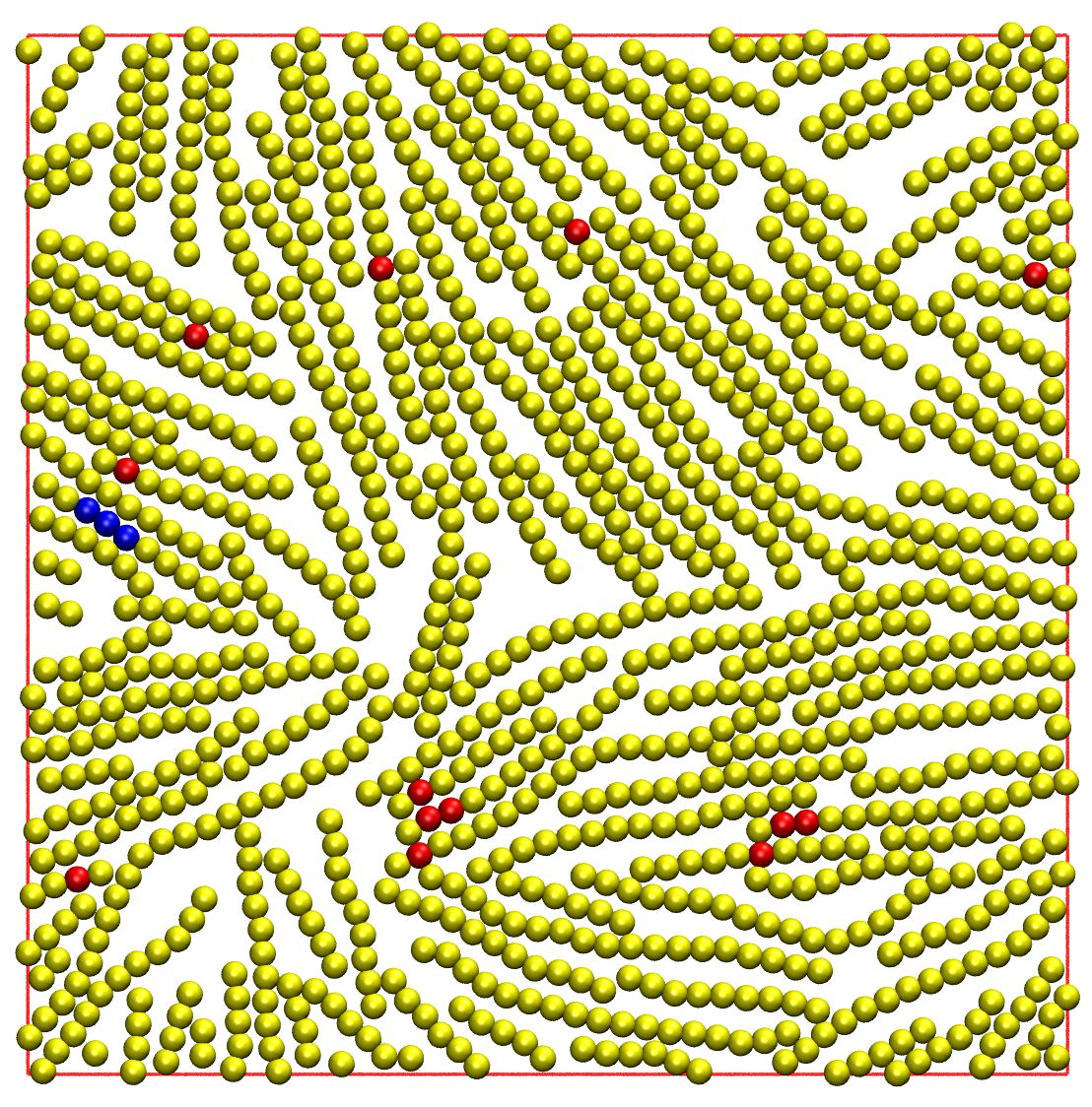
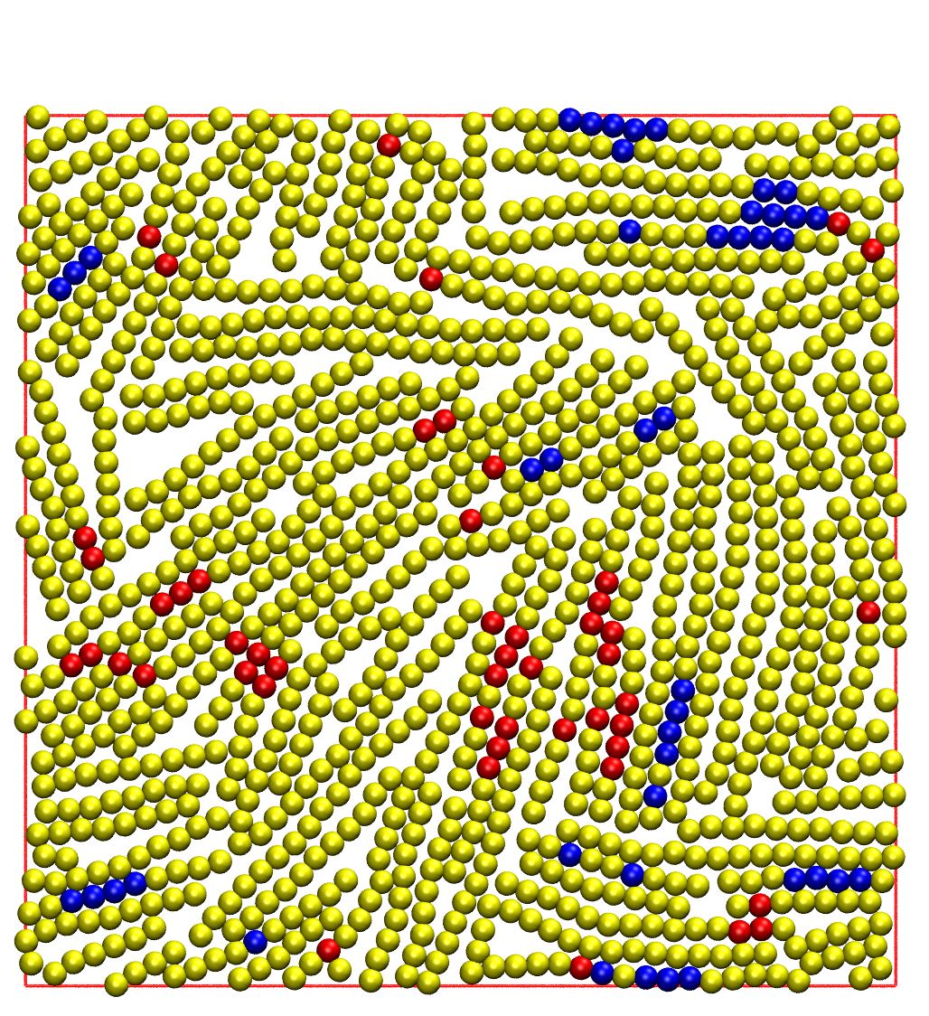


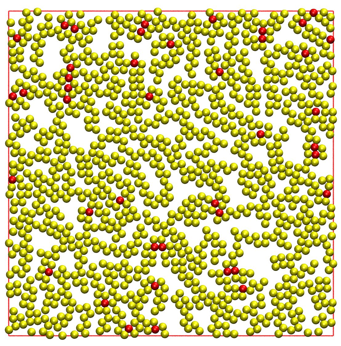
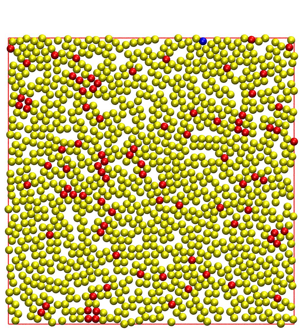
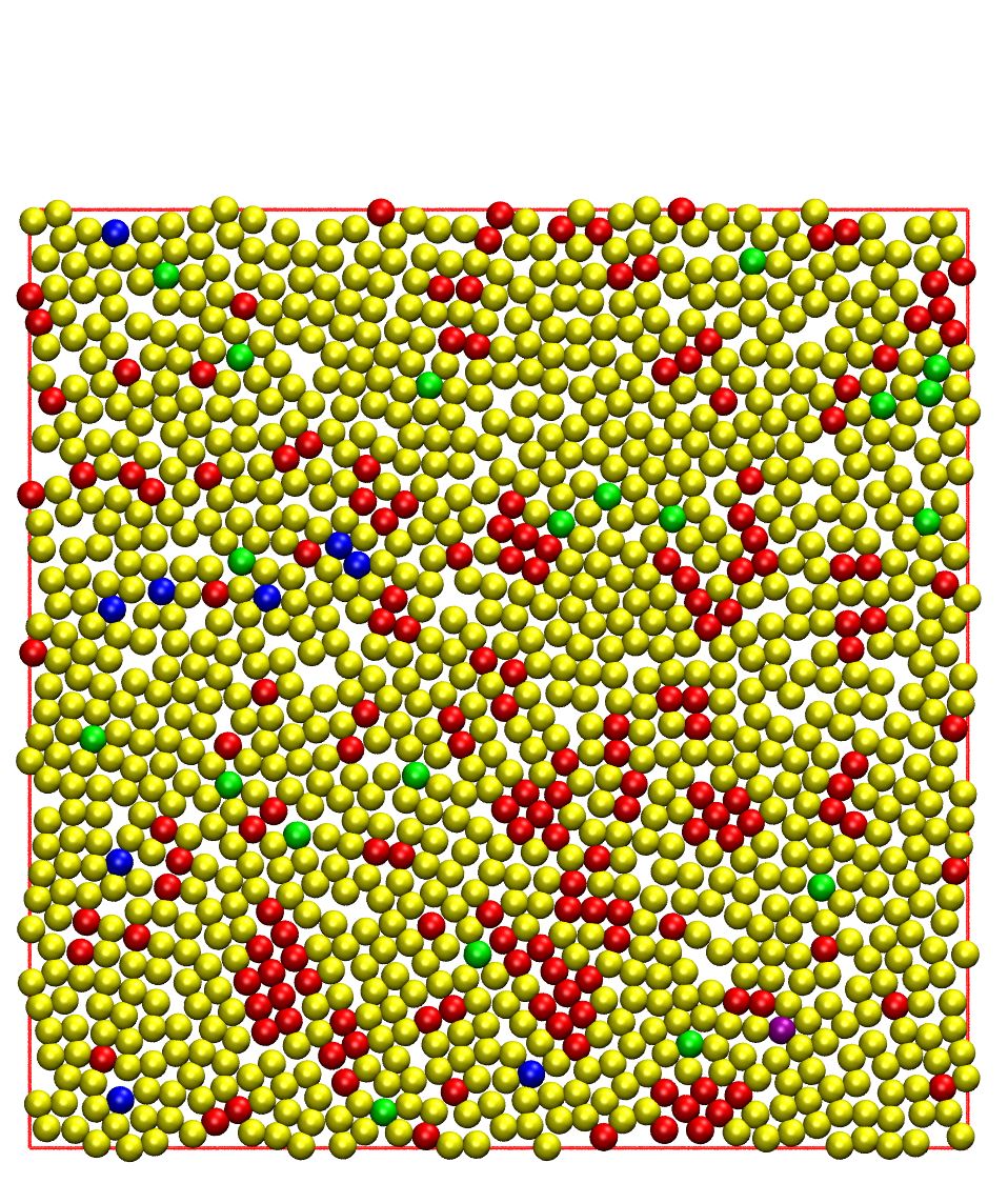

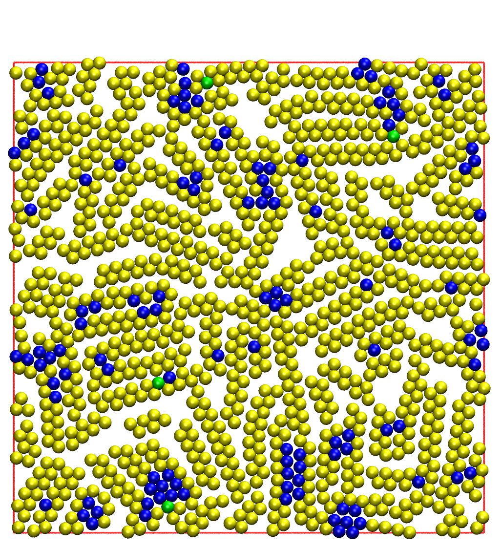
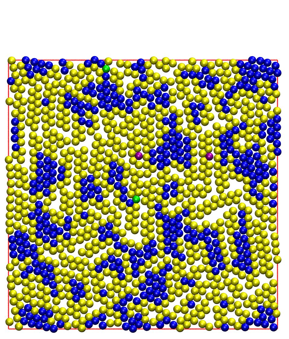
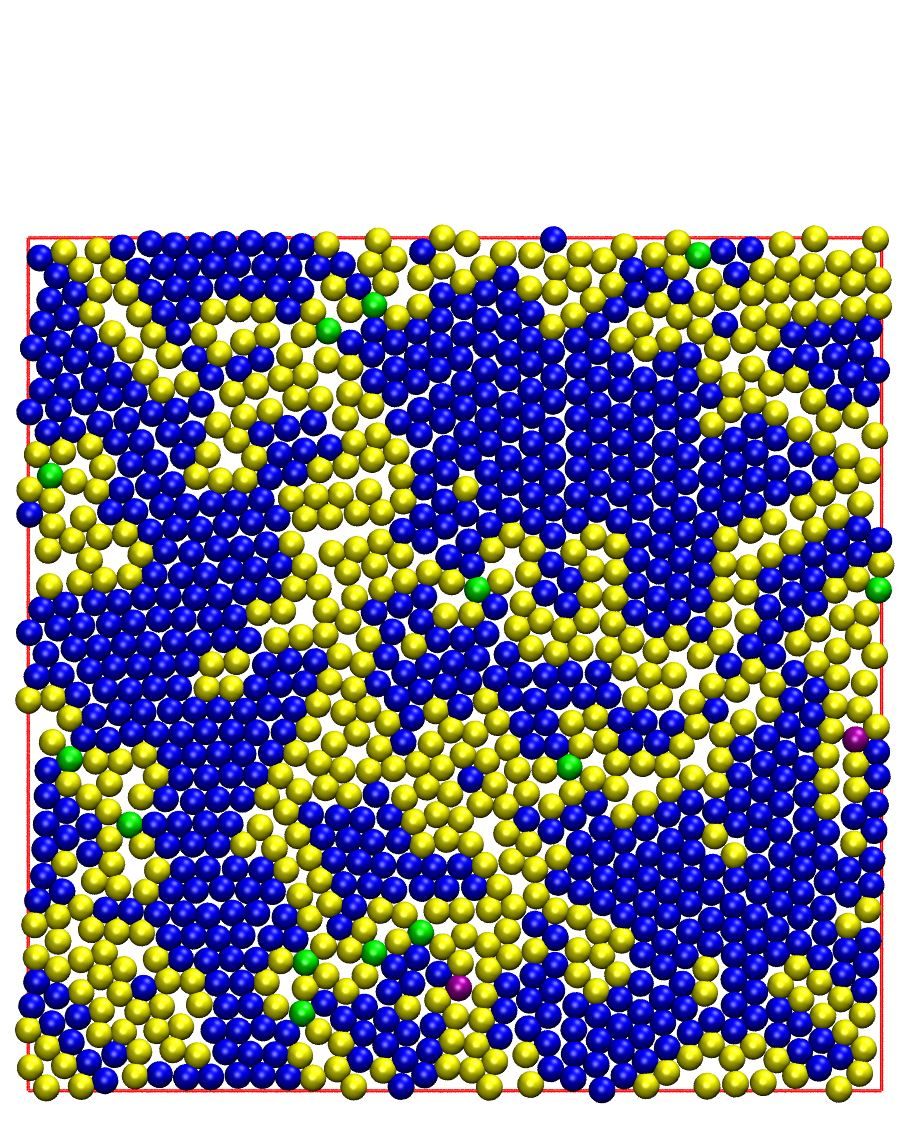
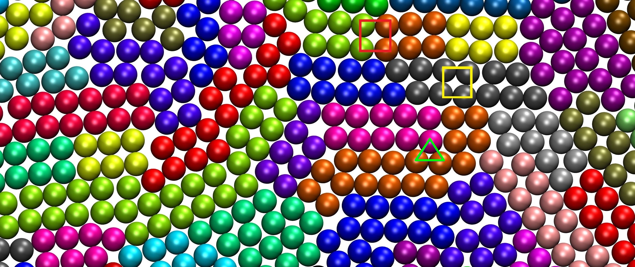
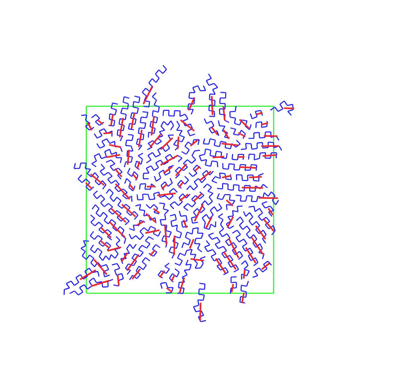
The only exception to the general trend dictating that RCP shows the highest local order is the system of right-angle chains. This is expected given that is incompatible with the geometry of the adjacent sites in the TRI crystal. Furthermore, the bending constant ( rad-2) is strong enough so that it does not allow large angle distortions which could lead to bending conformations of 60 or , which are elements of the TRI crystal connectivity. It is interesting to notice that visual inspection of the CCE-based snapshots for the right-angle chains in Fig. 5 reveals that at , 0.60 and 0.70, while the system is predominantly amorphous, the isolated ordered sites form SQU crystallites and the higher the concentration the higher the SQU order. However, as the system transits to the RCP state the pattern changes drastically, the SQU sites disappear almost completely and get replaced by small clusters of TRI character. As the RCP density is higher than that of the pure SQU crystal the resulting packing is necessarily a tiling pattern which is effectively a blend of intra-molecular square packing, imposed by the right-angle constraint, and inter-molecular chain alignments which fill the gaps in the square spacing to maximize local density. The net result is a configuration which is on one hand denser than the SQU crystal but on the other hand significantly less ordered, at least with respect to the tested SQU and TRI reference crystals. This can be clearly seen in the structural detail of Fig. 6 corresponding to a segment of the polymer packing at . Sphere monomers are colored according to the parent polymer so as to identify the intra- and inter-chain local arrangements. Square and triangle shapes are drawn to indicate the formation of intra- and inter-molecular squares and of intermolecular triangles filling the gaps between the vertices of the squares. Also, it can be seen that a significant fraction of the squares is distorted because bending angles follow a distribution around the equilibrium right angle, as shown in Fig. 2.
IV.4 Global Structure: Nematic and Tetratic Order Parameter
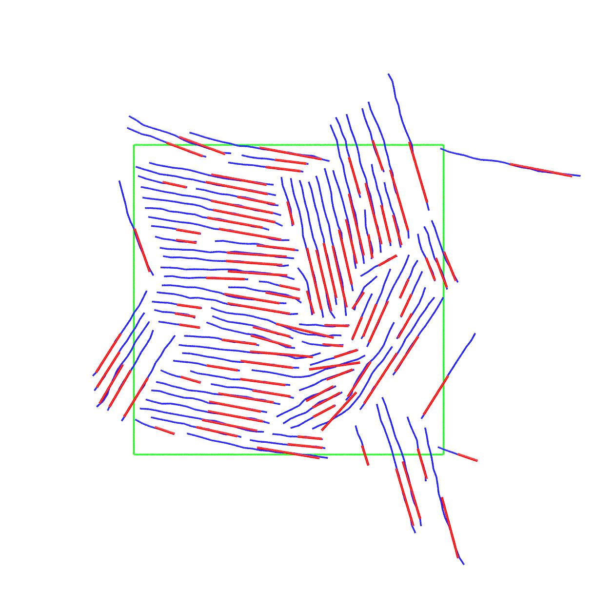
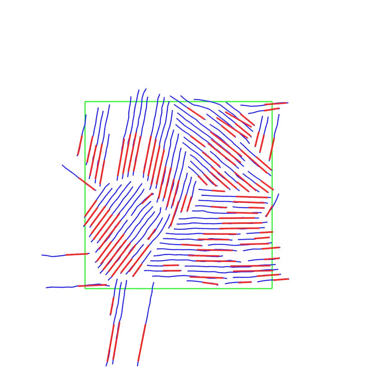
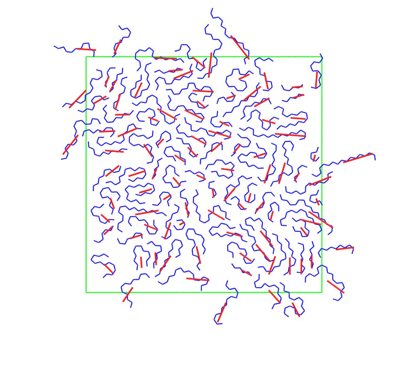
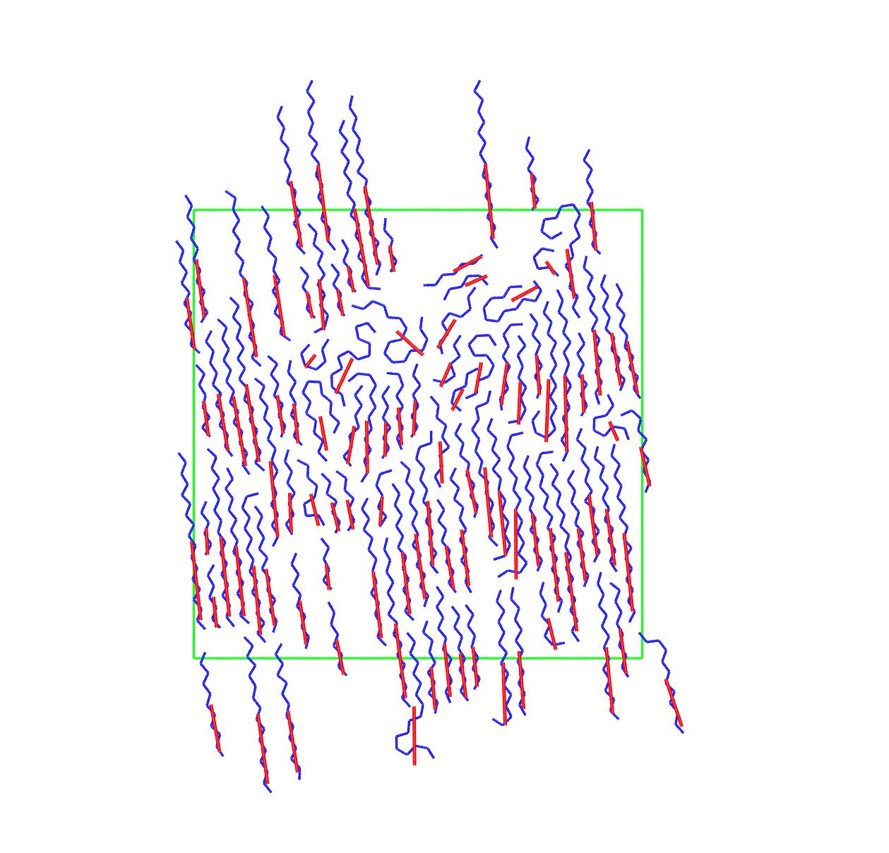
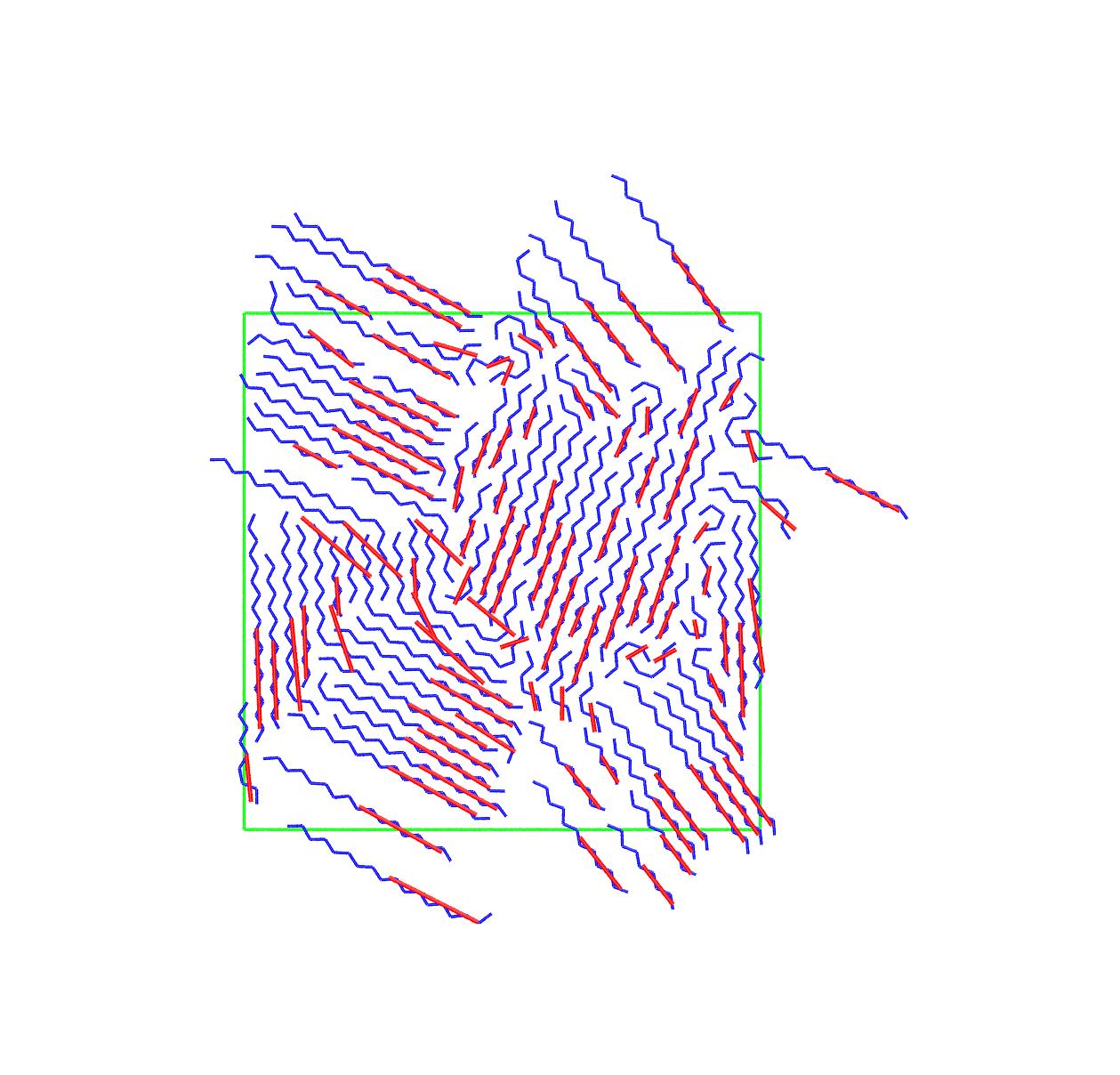
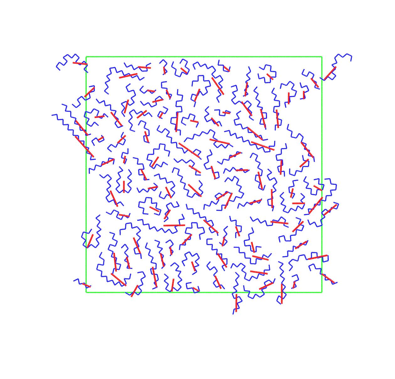
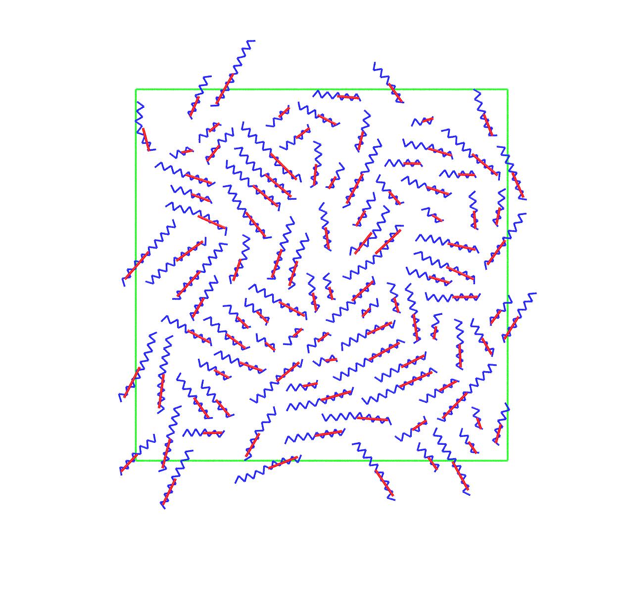
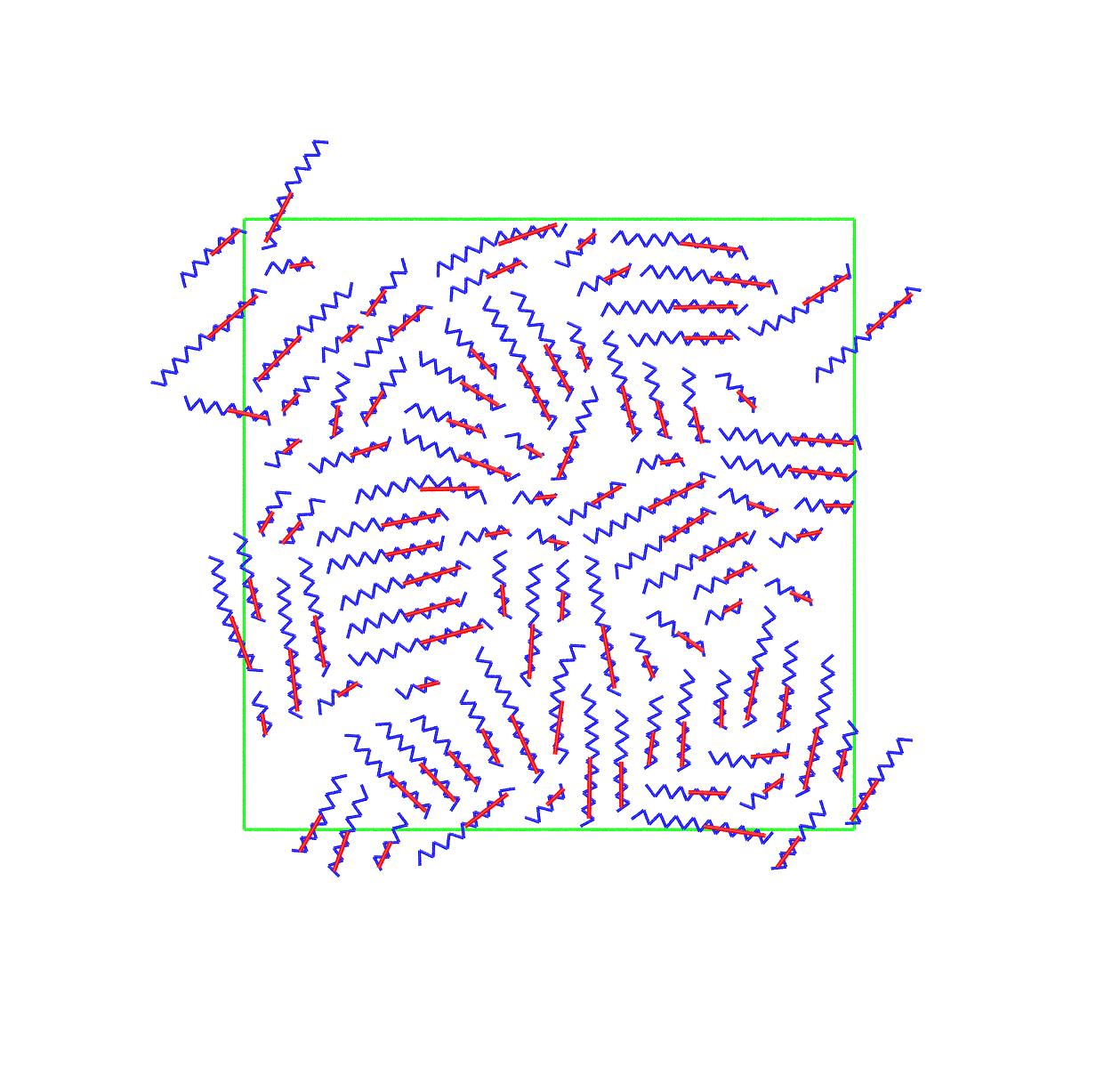
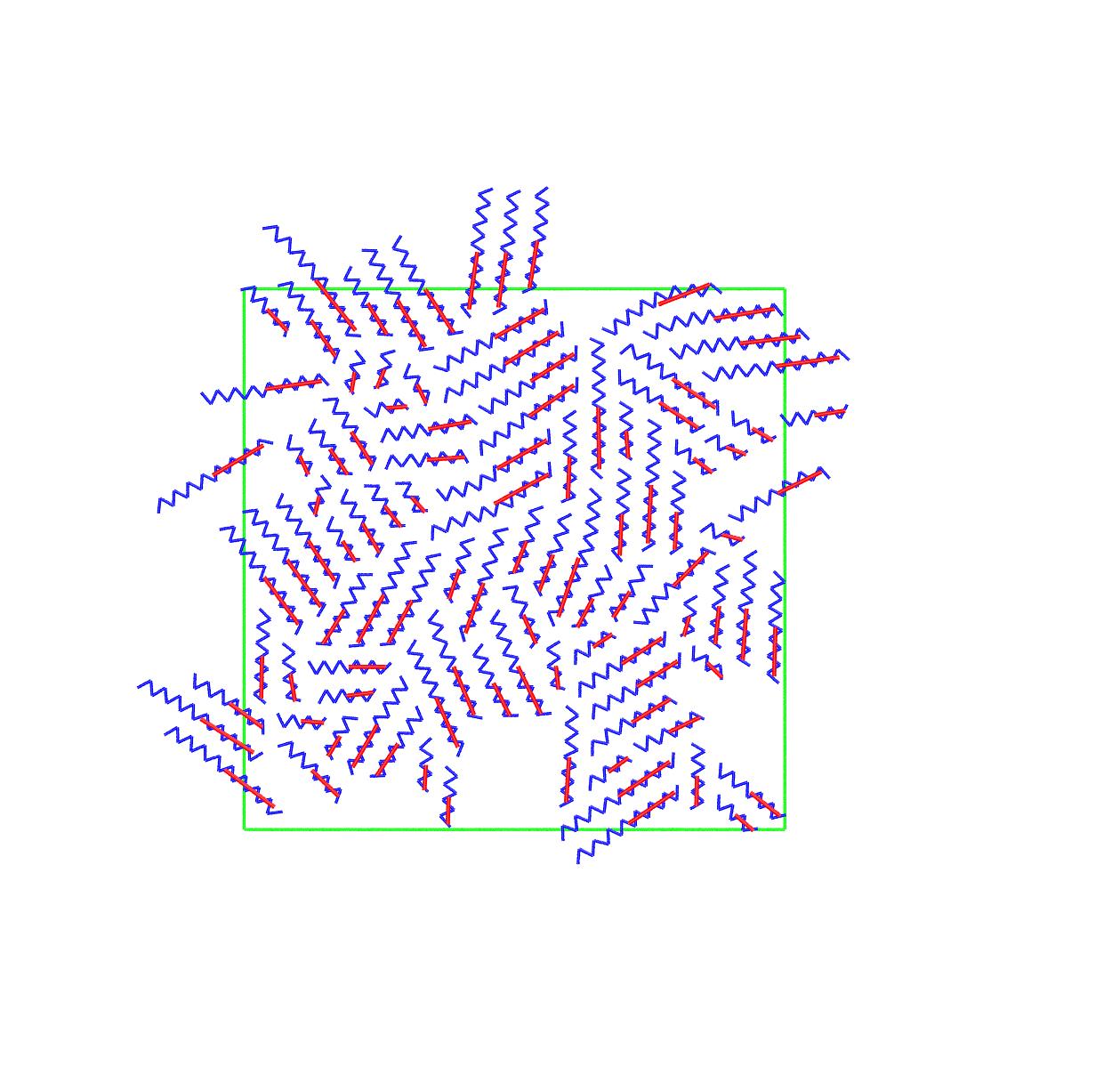
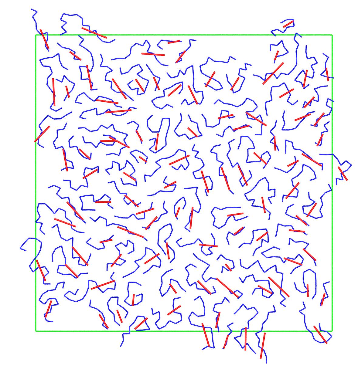
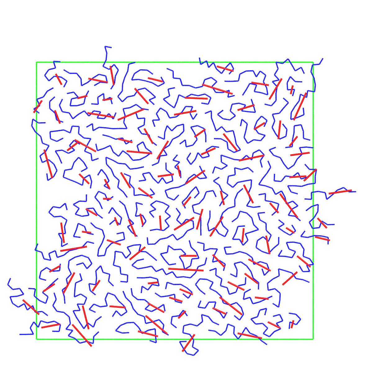
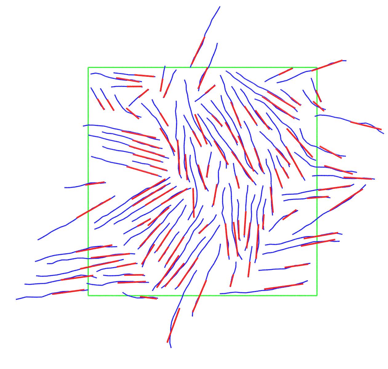
Figs. 7 and 8 show snapshots at the end of the MC simulations on semi- and fully-flexible polymers, respectively, where chains, shown in blue, are represented by lines. Also shown in red is the vector of the largest (semi)axis of the inertia ellipsoid, as calculated from the eigenvectors of the mass-moment of inertia tensor Karayiannis, Foteinopoulou, and Laso (2009a), with a length proportional to the length of the (semi)axis. Visual inspection of the final system configurations reveals a wealth of distinct global behavior ranging from isotropic state to the establishment of nematic and tetratic phases of varied level of perfection.
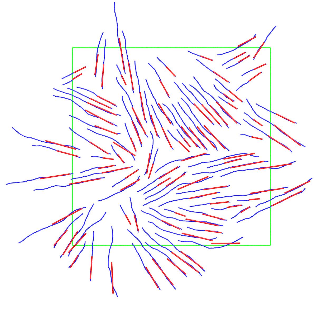
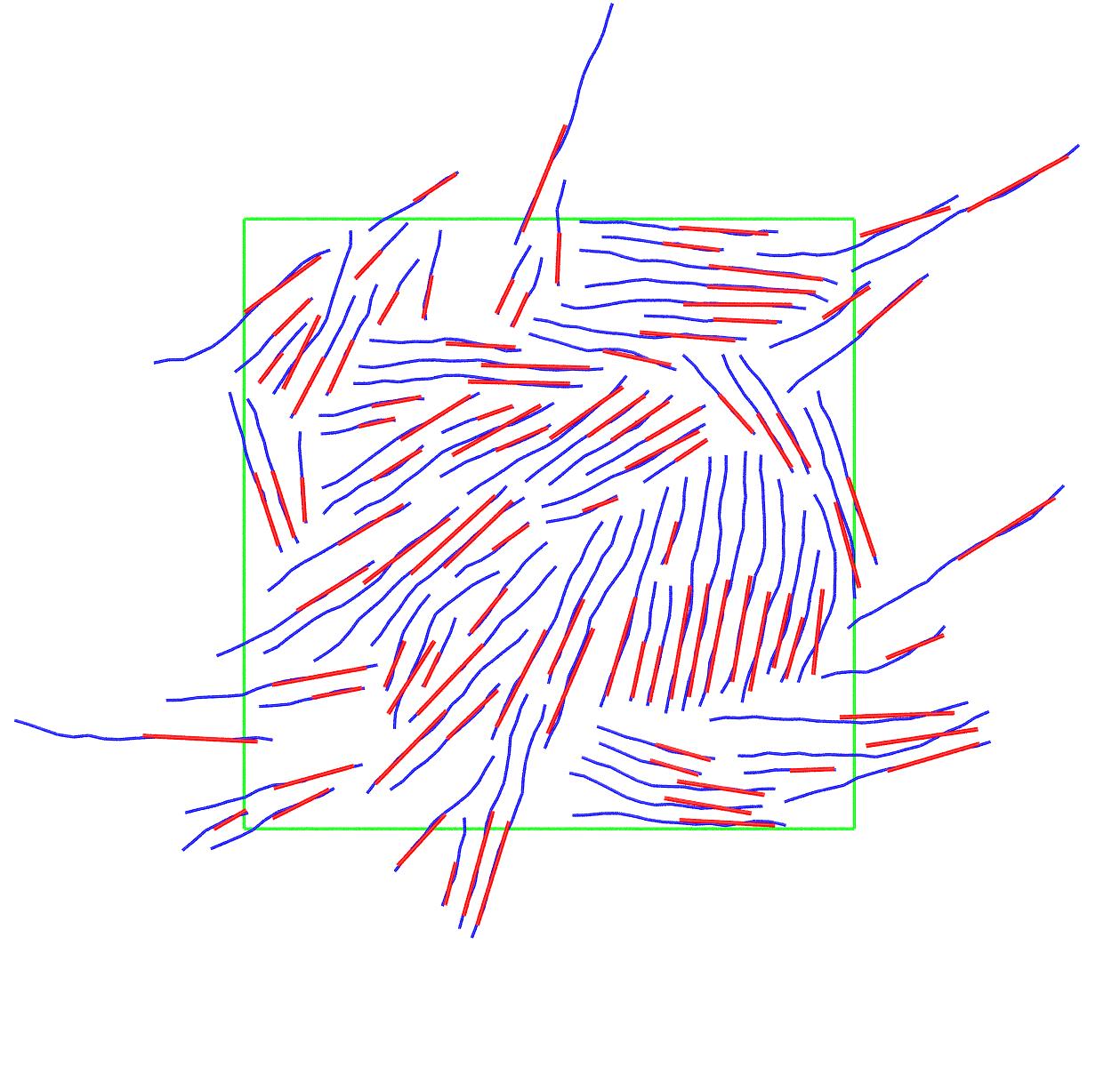
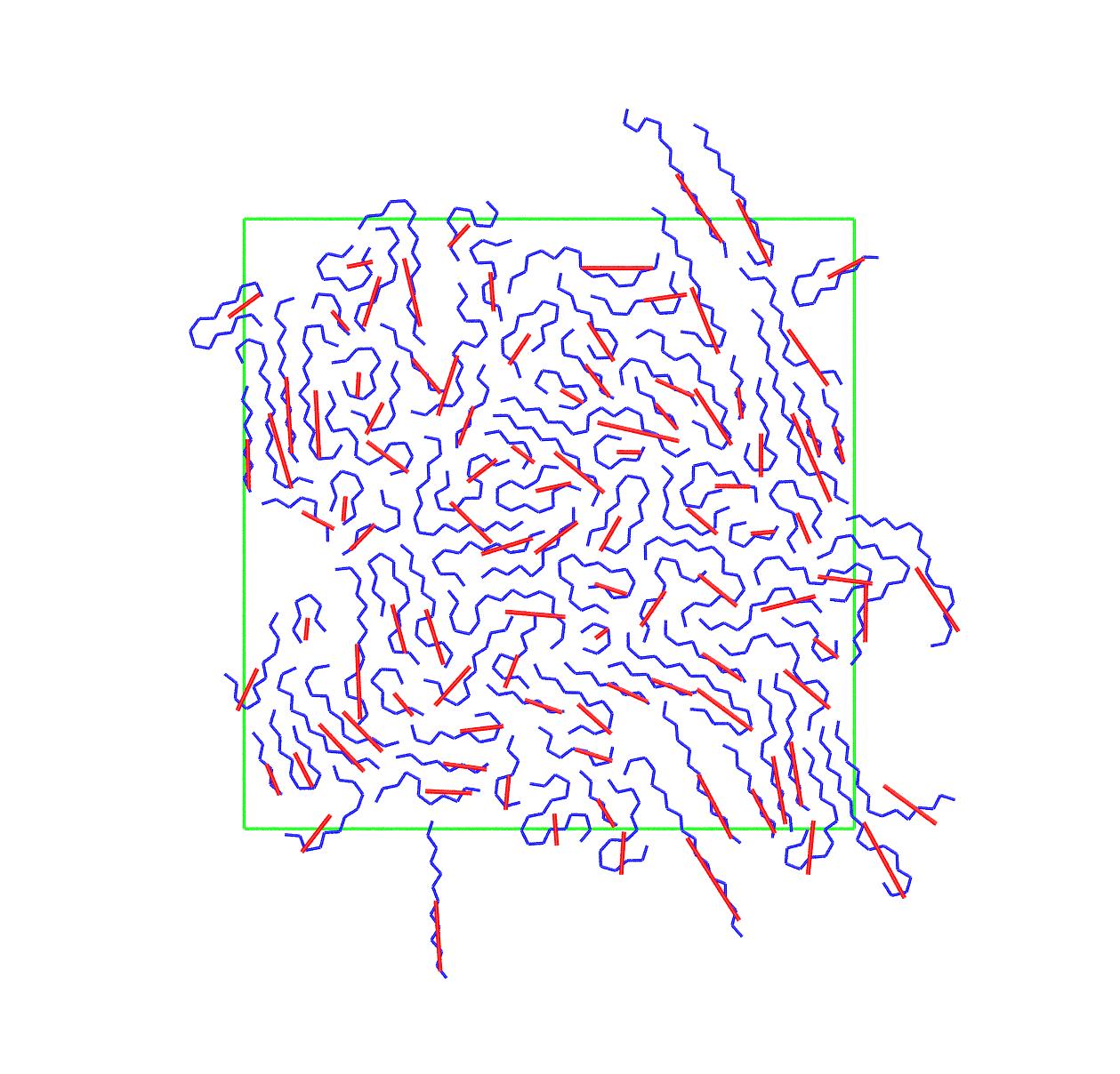

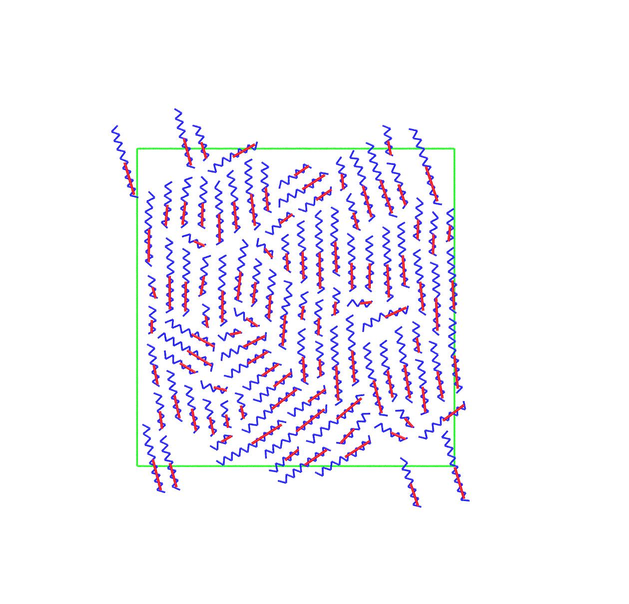

Interesting trends can be established from the evolution of the nematic () and tetratic () order parameters as a function of equilibrium bending angle and surface coverage. Starting with the most trivial behavior, the right-angle chains () remain isotropic at all packing densities, since for all frames. We should note here that for all isotropic systems in two dimensions and due to finite system size the long-range order parameters, be or , adopt positive values, which are expected to vanish in the limit of an infinitely-large system as originally discussed in Ref. Frenkel and Eppenga (1985).
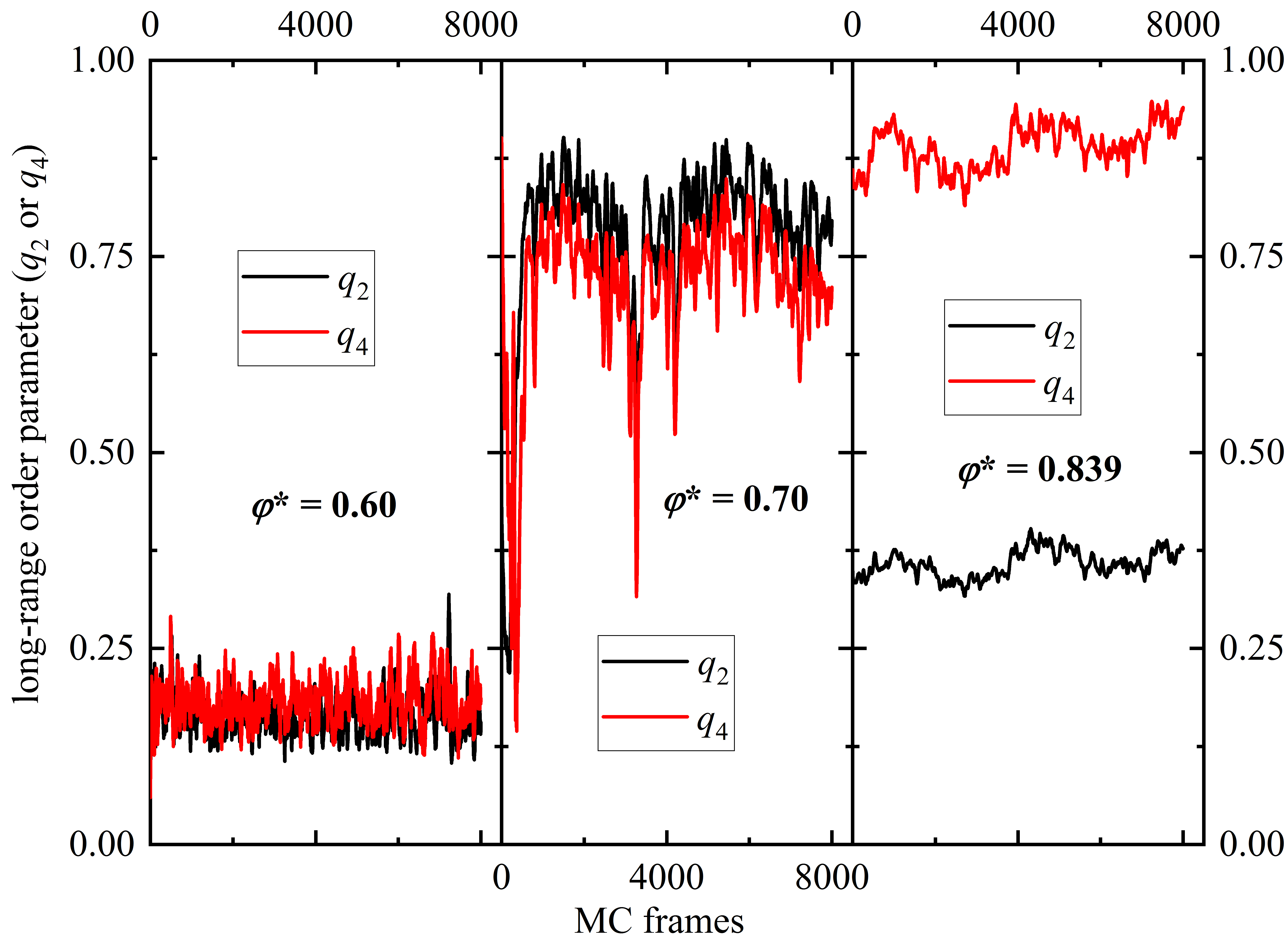
The rest of polymer systems demonstrate, with minor deviations, a unified dependence on surface coverage. First, at intermediate volume fractions ( and 0.60) the rod-like chains show a clear isotropic nematic transition, as indicated by the sharp increase in in the central panel of Fig. 9, where the system starts from an isotropic state () and very rapidly becomes nematic (). The resulting nematic phase is, however, unstable as evidenced by the very large fluctuations of the nematic order parameter as a function of MC frames. This instability is mainly attributed to the small chain lengths studied here leading to low aspect ratios for the polymers. As explained earlier, around of the chain population have an aspect ratio which can be considered below the stability threshold of for the nematic state in two dimensions as gauged in Bates and Frenkel (2000b) for regular rods, where is the length (fluctuating here) and the diameter (fixed here). Visualizations of the systems snapshots corresponding to the lowest and highest values can be seen in the left and right panels of Fig. 9 further confirming the instability of the nematic phase for rod-like chains. The formation of the unstable nematic state is evident also at higher volume fractions of and 0.70, with the latter configuration being more defect-ridden (lower ) compared to the former. However, at RCP the physical picture changes completely as rod-like chains adopt a highly imperfect tetratic phase since systematically and and as can be visually confirmed by the corresponding snapshot in the top-right panel of Fig. 7.
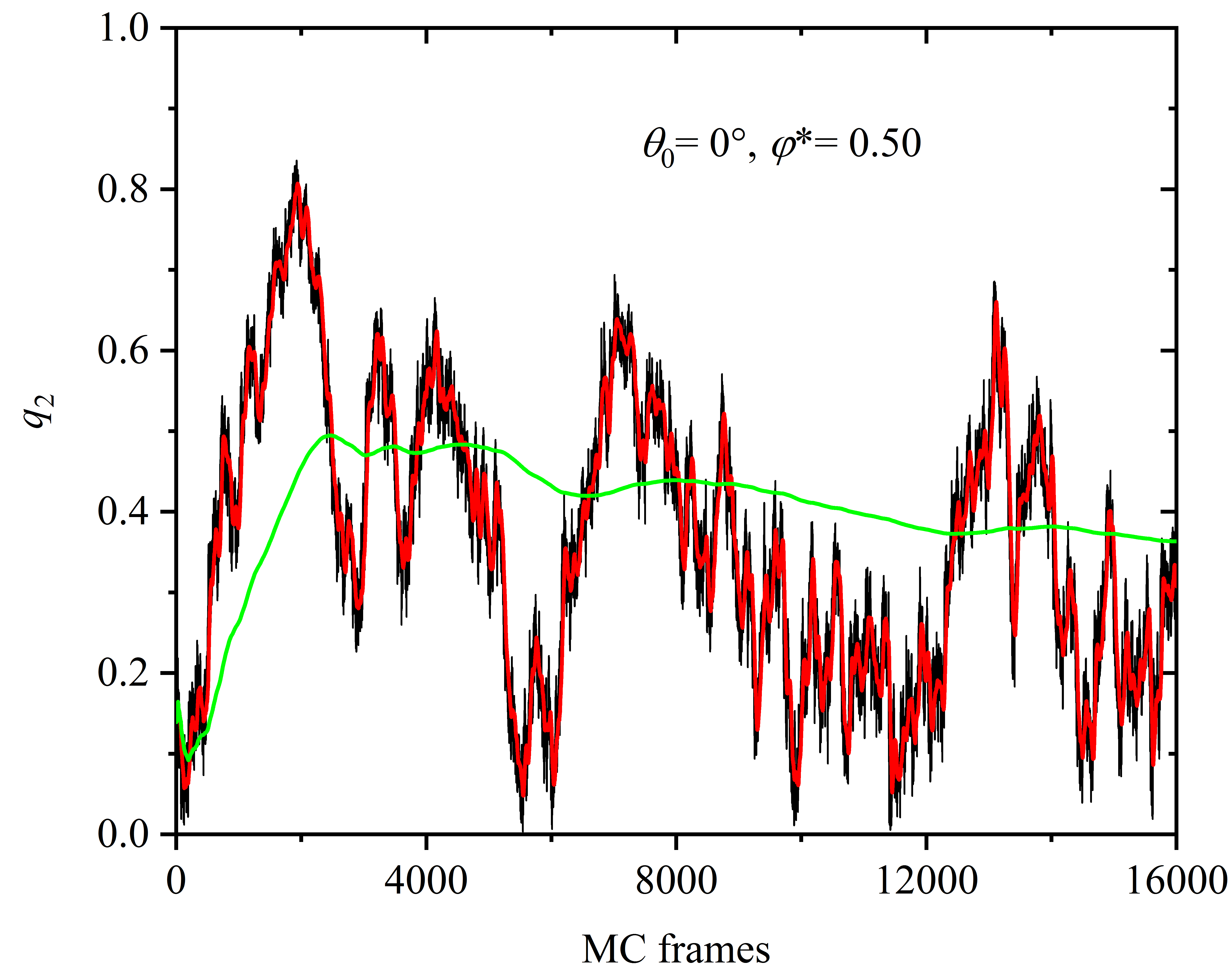
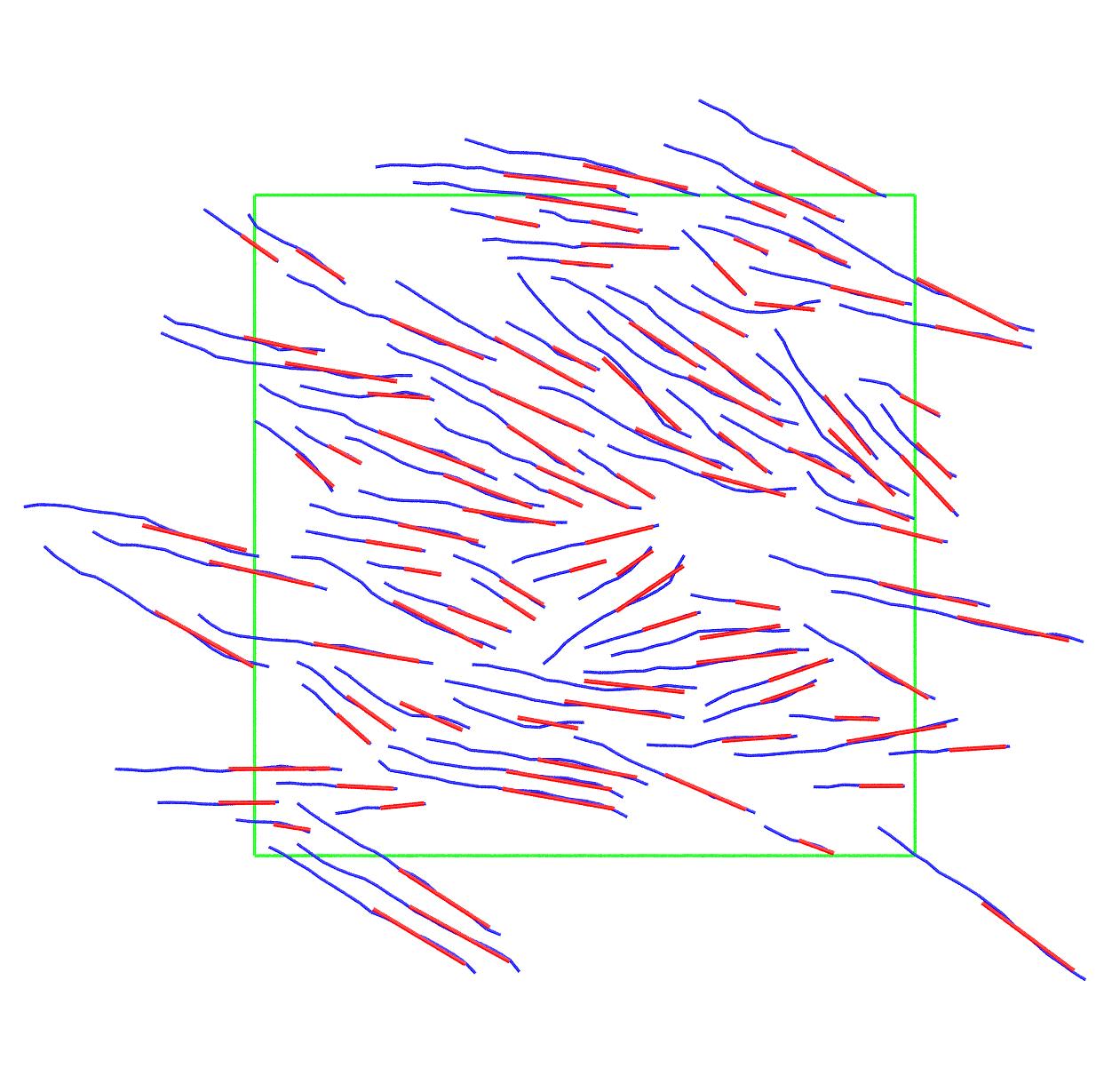
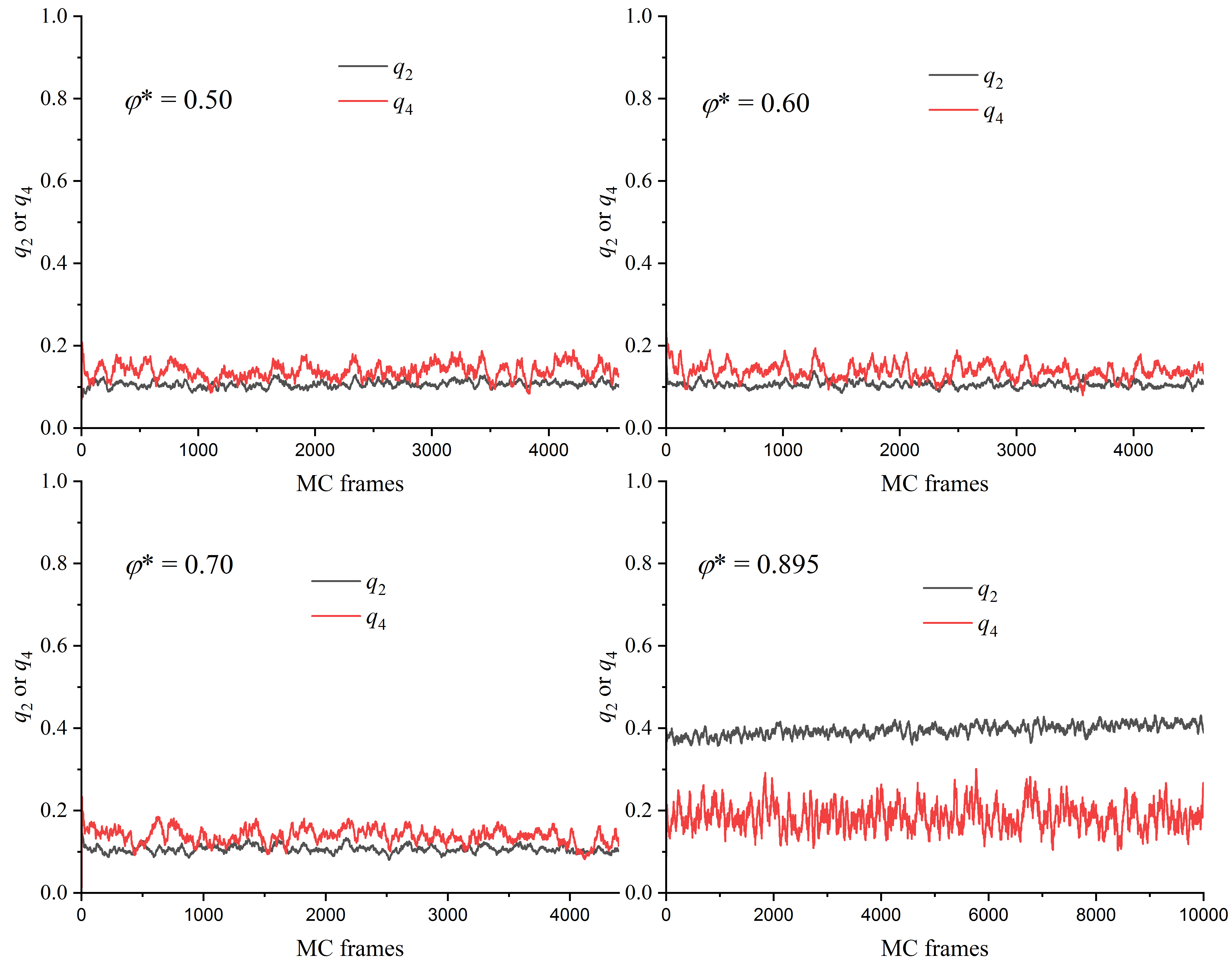
The extended () and compact () zig-zag chains exhibit an almost identical behavior: at both systems remain isotropic, while at higher concentrations ( and 0.70) they transit to a stable nematic phase, being characterized by simultaneously high values of and . Finally, at the RCP limit the tetratic state is established, being identified by high values for (tetratic order parameter) and significantly lower ones for (nematic order parameter). As a typical paradigm, the evolution of and versus MC frames for the at , 0.70 and 0.839 (= ), corresponding to isotropic, nematic and tetratic states, can be found in the panels of Fig. 10. These trends are confirmed by the system configurations at the end of the simulations shown in Fig. 7 where parallel and perpendicular inter-chain arrangements are visible.
In comparison, as seen in Fig. 11, the fully flexible chains show isotropic behavior over the whole concentration range with a small increase in the nematic order occuring at RCP(FJ). This ordering is a rather localized trend, occuring in a small sub-group of chains (rightmost panel of Fig. 8.)
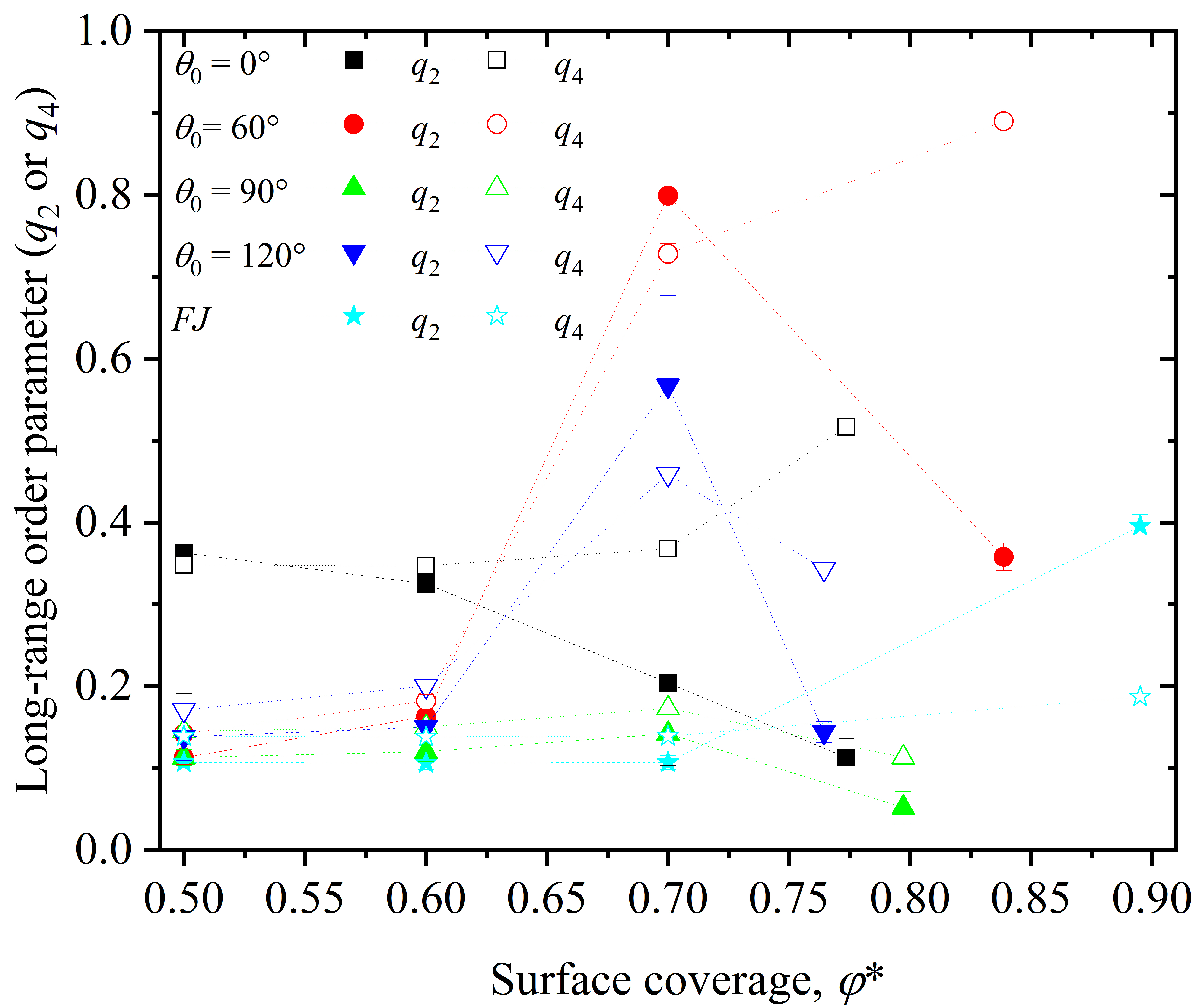
The results on the local and global order, as the RCP limit in two dimensions is approached, are summarized in Fig. 12 showing the dependence of (left panel) the degree of crystallinity, , and (right panel) of (filled symbols) and (open symbols) on surface coverage for all equilibrium bending angles studied here, which include the data for fully flexible (FJ) chains.
The right-angle chains obviously constitute a singular case, due to being incompatible with the site geometry of the TRI crystal. Consequently, both their local and global order parameters are characterized by very low values over the whole concentration range, corresponding to a locally disordered and globally isotropic system. For the rest of the systems local order increases significantly with packing density and in all cases the RCP limit is characterized by the highest observed degree of crystallinity. However, the same is not true for global order: semi-flexible chains show the following long-range structural transition as RCP is approached: isotropic nematic tetratic. The nematic order of rod-like chains with average length is highly unstable as demonstrated also by the very large error bars seen in Fig. 12, while the tetratic state seems to be an identifying characteristic of the RCP limit.

V Conclusions
Through extensive simulations we have studied the packing ability, local and global structure of semi-flexible athermal polymers extremely confined in monolayers, practically corresponding to systems in two dimensions. The combination of extreme confinement and very high surface coverage leads to a rich structural behavior as a function of equilibrium bending angle.
As a first result we identify the trends on the densest configurations according to which: . Simple calculations show that in three dimensions the RCP limit is approximately 13.6% less dilute compared to the maximum achievable density of the HCP and FCC ideal crystals. In two dimensions and based on the present findings, the RCP limits range from the highest one of the freely-jointed (FJ) chains, which is just 1.3% lower than the maximum achievable surface coverage, corresponding to the TRI crystal, to the least dense one of the compact, zig-zag chain configurations of (approximately 15.8% less concentrated than ).
The packing ability is intimately related to the bond geometry of the chains and their size, as imposed primarily by the equilibrium bending angle and secondarily by the surface coverage. A critical component in the identification of the RCP limit is the quantification of the inherent degree of order. Thus, order is here the combined contribution of local order at the level of monomers (crystallinity) and of global order at the level of chains.
A wealth of distinct behaviors but also some universal trends can be recognized. Packings of right-angle (), chains show a singular behavior by remaining amorphous (disordered) at the local level and isotropic at the level of chains. Interestingly enough, the RCP limit for right-angle chains exceeds the maximum surface coverage of an ideal square crystal, i.e. . In parallel, the equilibrium bending angle of is incompatible with the geometric elements of the TRI crystal and thus this combination explains the disordered/isotropic state of the right-angle chain packing. Universal behavior is observed for the rest of semi-flexible systems: first, crystallinity increases monotonically as concentration increases and reaches its maximum at the RCP limit. This is in sharp contrast with the corresponding trends in three dimensions where disorder prevails at the RCP limit. Factors that lead to this discrepancy can be attributed to the protocol dependent nature of the RCP limit (which we should note is the same for all chain systems simulated here) in 2D and 3D, but also to the difficulty of crystal formation in 3D compared to 2D due to the increased coordination number at sufficiently high densities.
Perhaps the most interesting trend is observed with respect to the global order. For rod-like polymers, and given the short chain lengths studied here, the nematic phase is highly unstable, fluctuating between configurations of high nematic order and ones of high tetratic order. Zig-zag chains of acute or obtuse supplementary angles show the following transition as surface coverages increases: isotropic nematic tetratic order, with the latter being the prevailing state at the RCP limit. Thus, based on the descriptors of order utilized here we can claim that it is the tetratic order that is intimately related to the establishment of random close packing in two dimensions for polymers.
Based on the results presented here athermal polymers in two dimensions possess a richness of multi-scale structural behavior which is not encountered in their monomeric analogs and which appears even more complex than the one exhibited by the 3D analogs under bulk conditions.
Acknowledgements.
Authors acknowledge support through project "PID2021-127533NB-I00" of MICINN/FEDER (Ministerio de Ciencia e Innovación, Fondo Europeo de Desarrollo Regional). D.M.F. acknowledges financial support through “Programa Propio UPM Santander” of Universidad Politécnica de Madrid (UPM) and Santander Bank. The authors gratefully acknowledge UPM for providing computing resources on the Magerit supercomputer through projects “r727”, “s341”, “t736” and “u242”.Author Declarations
Conflict of Interest
The authors have no conflicts to disclose.
Author Contributions
Daniel Martínez-Fernández: Data curation (lead); Formal analysis (equal); Investigation (equal); Software (equal); Visualization (equal); Writing – original draft (equal).
Clara Perdosa: Data curation (equal); Formal analysis (equal); Investigation (equal); Software (supporting); Visualization (supporting); Writing – review & editing (equal).
Miguel Herranz: Data curation (supporting); Formal analysis (supporting); Investigation (supporting); Software (equal); Writing – review & editing (equal).
Katerina Foteinopoulou: Formal analysis (equal); Methodology (equal); Validation (lead); Writing – review & editing (equal); Funding Acquisition (equal).
Nikos Ch. Karayiannis: Conceptualization (lead); Funding acquisition (equal); Investigation (equal); Methodology (equal); Writing – original draft (equal).
Manuel Laso: Methodology (equal); Funding acquisition (equal); Writing – review & editing (equal); Funding Acquisition (equal).
Data Availability Statement
The data that support the findings of this study are available from the corresponding author upon reasonable request.
References
- Yuan et al. (2022) Y. K. Yuan, D. S. Kim, J. H. Zhou, D. J. Chang, F. Zhu, Y. Nagaoka, Y. Yang, M. Pham, S. J. Osher, O. Chen, P. Ercius, A. K. Schmid, and J. W. Miao, “Three-dimensional atomic packing in amorphous solids with liquid-like structure,” Nature Materials 21, 95–+ (2022).
- Gaines et al. (2016) J. C. Gaines, W. W. Smith, L. Regan, and C. S. O’Hern, “Random close packing in protein cores,” Physical Review E 93 (2016), 10.1103/PhysRevE.93.032415.
- Conway and Sloane (1999) J. H. Conway and N. J. A. Sloane, Sphere Packings, Lattices and Groups, 3rd ed., Vol. 290 (Springer New York, New York, NY, 1999).
- Manoharan (2015) V. N. Manoharan, “Colloidal matter: Packing, geometry, and entropy,” Science 349 (2015), 10.1126/science.1253751.
- Börzsönyi et al. (2016) T. Börzsönyi, E. Somfai, B. Szabó, S. Wegner, P. Mier, G. Rose, and R. Stannarius, “Packing, alignment and flow of shape-anisotropic grains in a 3d silo experiment,” New Journal of Physics 18 (2016), 10.1088/1367-2630/18/9/093017.
- Weaire and Aste (2008) W. Weaire and T. Aste, The Pursuit of Perfect Packing (Taylor and Francis, New York, 2008).
- Sheng et al. (2006) H. W. Sheng, W. K. Luo, F. M. Alamgir, J. M. Bai, and E. Ma, “Atomic packing and short-to-medium-range order in metallic glasses,” Nature 439, 419–425 (2006).
- Cai et al. (2021) Z. Y. Cai, Z. W. Li, S. Ravaine, M. X. He, Y. L. Song, Y. D. Yin, H. B. Zheng, J. H. Teng, and A. O. Zhang, “From colloidal particles to photonic crystals: advances in self-assembly and their emerging applications,” Chemical Society Reviews 50, 5898–5951 (2021).
- Boles, Engel, and Talapin (2016) M. A. Boles, M. Engel, and D. V. Talapin, “Self-assembly of colloidal nanocrystals: From intricate structures to functional materials,” Chemical Reviews 116, 11220–11289 (2016).
- Baranau and Tallarek (2014) V. Baranau and U. Tallarek, “Random-close packing limits for monodisperse and polydisperse hard spheres,” Soft Matter 10, 3826–3841 (2014).
- Atkinson, Stillinger, and Torquato (2014) S. Atkinson, F. H. Stillinger, and S. Torquato, “Existence of isostatic, maximally random jammed monodisperse hard-disk packings,” Proceedings of the National Academy of Sciences of the United States of America 111, 18436–18441 (2014).
- Torquato and Stillinger (2001) S. Torquato and F. H. Stillinger, “Multiplicity of generation, selection, and classification procedures for jammed hard-particle packings,” Journal of Physical Chemistry B 105, 11849–11853 (2001).
- Lubachevsky and Stillinger (1990) B. D. Lubachevsky and F. H. Stillinger, “Geometric-properties of random disk packings,” Journal of Statistical Physics 60, 561–583 (1990).
- Meyer et al. (2010) S. Meyer, C. M. Song, Y. L. Jin, K. Wang, and H. A. Makse, “Jamming in two-dimensional packings,” Physica a-Statistical Mechanics and Its Applications 389, 5137–5144 (2010).
- Hinrichsen, Feder, and Jossang (1990) E. L. Hinrichsen, J. Feder, and T. Jossang, “Random packing of disks in 2 dimensions,” Physical Review A 41, 4199–4209 (1990).
- Blumenfeld (2021) R. Blumenfeld, “Disorder criterion and explicit solution for the disc random packing problem,” Physical Review Letters 127 (2021), 10.1103/PhysRevLett.127.118002.
- Jin, Puckett, and Makse (2014) Y. L. Jin, J. G. Puckett, and H. A. Makse, “Statistical theory of correlations in random packings of hard particles,” Physical Review E 89 (2014), 10.1103/PhysRevE.89.052207.
- Zaccone (2022) A. Zaccone, “Explicit analytical solution for random close packing in d=2 and d=3,” Physical Review Letters 128 (2022), 10.1103/PhysRevLett.128.028002.
- Cheng (2010) X. Cheng, “Packing structure of a two-dimensional granular system through the jamming transition,” Soft Matter 6, 2931–2934 (2010).
- Martiniani et al. (2017) S. Martiniani, K. J. Schrenk, K. Ramola, B. Chakraborty, and D. Frenkel, “Numerical test of the edwards conjecture shows that all packings are equally probable at jamming,” Nature Physics 13, 848–+ (2017).
- Richard et al. (1999) P. Richard, A. Gervois, L. Oger, and J. P. Troadec, “Order and disorder in hard-sphere packings,” Europhysics Letters 48, 415–420 (1999).
- Heitkam, Drenckhan, and Frohlich (2012) S. Heitkam, W. Drenckhan, and J. Frohlich, “Packing spheres tightly: Influence of mechanical stability on close-packed sphere structures,” Physical Review Letters 108 (2012), 10.1103/PhysRevLett.108.148302.
- Noya and Almarza (2015) E. G. Noya and N. G. Almarza, “Entropy of hard spheres in the close-packing limit,” Molecular Physics 113, 1061–1068 (2015).
- Finney (1970) J. L. Finney, “Random packings and structure of simple liquids .1. geometry of random close packing,” Proceedings of the Royal Society of London Series a-Mathematical and Physical Sciences 319, 479–493 (1970).
- Scott and Kilgour (1969) G. D. Scott and D. M. Kilgour, “Density of random close packing of spheres,” Journal of Physics D-Applied Physics 2, 863– (1969).
- Conway and Sloane (1998) J. Conway and N. Sloane, Sphere Packings, Lattices and Groups (Springer Verlag, New York, 1998).
- Bernal and Finney (1967) J. D. Bernal and J. L. Finney, “Random close-packed hard-sphere model .2. geometry of random packing of hard spheres,” Discussions of the Faraday Society 43, 62–69 (1967).
- Medvedev, Bezrukov, and Shtoyan (2004) N. N. Medvedev, A. Bezrukov, and D. Shtoyan, “From amorphous solid to defective crystal. a study of structural peculiarities in close packings of hard spheres,” Journal of Structural Chemistry 45, S23–S30 (2004).
- Luchnikov et al. (2002) V. Luchnikov, A. Gervois, P. Richard, L. Oger, and J. P. Troadec, “Crystallization of dense hard sphere packings - competition of hcp and fcc close order,” Journal of Molecular Liquids 96-7, 185–194 (2002).
- Xu, Blawzdziewicz, and O’Hern (2005) N. Xu, J. Blawzdziewicz, and C. S. O’Hern, “Random close packing revisited: Ways to pack frictionless disks,” Physical Review E 71 (2005), 10.1103/PhysRevE.71.061306.
- Kamien and Liu (2007) R. D. Kamien and A. J. Liu, “Why is random close packing reproducible?” Physical Review Letters 99 (2007), 10.1103/PhysRevLett.99.155501.
- Donev, Stillinger, and Torquato (2005) A. Donev, F. H. Stillinger, and S. Torquato, “Unexpected density fluctuations in jammed disordered sphere packings,” Physical Review Letters 95 (2005), 10.1103/PhysRevLett.95.090604.
- Anikeenko and Medvedev (2007) A. V. Anikeenko and N. N. Medvedev, “Polytetrahedral nature of the dense disordered packings of hard spheres,” Physical Review Letters 98 (2007), 10.1103/PhysRevLett.98.235504.
- Torquato, Truskett, and Debenedetti (2000) S. Torquato, T. M. Truskett, and P. G. Debenedetti, “Is random close packing of spheres well defined?” Physical Review Letters 84, 2064–2067 (2000).
- Desmond and Weeks (2009) K. W. Desmond and E. R. Weeks, “Random close packing of disks and spheres in confined geometries,” Physical Review E 80 (2009), 10.1103/PhysRevE.80.051305.
- Wöhler and Schilling (2022) W. Wöhler and T. Schilling, “Hard sphere crystal nucleation rates: Reconciliation of simulation and experiment,” Physical Review Letters 128 (2022), 10.1103/PhysRevLett.128.238001.
- Gasser (2009) U. Gasser, “Crystallization in three- and two-dimensional colloidal suspensions,” Journal of Physics-Condensed Matter 21 (2009), 10.1088/0953-8984/21/20/203101.
- Han et al. (2008) Y. Han, N. Y. Ha, A. M. Alsayed, and A. G. Yodh, “Melting of two-dimensional tunable-diameter colloidal crystals,” Physical Review E 77 (2008), 10.1103/PhysRevE.77.041406.
- Wojciechowski et al. (2003) K. W. Wojciechowski, K. V. Tretiakov, A. C. Branka, and M. Kowalik, “Elastic properties of two-dimensional hard disks in the close-packing limit,” Journal of Chemical Physics 119, 939–946 (2003).
- Hales et al. (2017) T. Hales, M. Adams, G. Bauer, T. D. Dang, J. Harrison, L. T. Hoang, C. Kaliszyk, V. Magron, S. McLaughlin, T. T. Nguyen, Q. T. Nguyen, T. Nipkow, S. Obua, J. Pleso, J. Rute, A. Solovyev, T. H. A. Ta, N. T. Tran, T. D. Trieu, J. Urban, K. Vu, and R. Zumkeller, “A formal proof of the kepler conjecture,” Forum of Mathematics Pi 5 (2017), 10.1017/fmp.2017.1.
- Ballesta, Duri, and Cipelletti (2008) P. Ballesta, A. Duri, and L. Cipelletti, “Unexpected drop of dynamical heterogeneities in colloidal suspensions approaching the jamming transition,” Nature Physics 4, 550–554 (2008).
- Unger, Kertesz, and Wolf (2005) T. Unger, J. Kertesz, and D. E. Wolf, “Force indeterminacy in the jammed state of hard disks,” Physical Review Letters 94 (2005), 10.1103/PhysRevLett.94.178001.
- Rissone, Corwin, and Parisi (2021) P. Rissone, E. I. Corwin, and G. Parisi, “Long-range anomalous decay of the correlation in jammed packings,” Physical Review Letters 127 (2021), 10.1103/PhysRevLett.127.038001.
- Chen, Zhang, and Glotzer (2007) T. Chen, Z. Zhang, and S. C. Glotzer, “A precise packing sequence for self-assembled convex structures,” Proceedings of the National Academy of Sciences of the United States of America 104, 717–722 (2007).
- Cinacchi and Torquato (2015) G. Cinacchi and S. Torquato, “Hard convex lens-shaped particles: Densest-known packings and phase behavior,” Journal of Chemical Physics 143 (2015), 10.1063/1.4936938.
- Atkinson, Jiao, and Torquato (2012) S. Atkinson, Y. Jiao, and S. Torquato, “Maximally dense packings of two-dimensional convex and concave noncircular particles,” Physical Review E 86 (2012), 10.1103/PhysRevE.86.031302.
- Torquato and Jiao (2012) S. Torquato and Y. Jiao, “Organizing principles for dense packings of nonspherical hard particles: Not all shapes are created equal,” Physical Review E 86 (2012), 10.1103/PhysRevE.86.011102.
- Haji-Akbari et al. (2013) A. Haji-Akbari, E. R. Chen, M. Engel, and S. C. Glotzer, “Packing and self-assembly of truncated triangular bipyramids,” Physical Review E 88 (2013), 10.1103/PhysRevE.88.012127.
- Torquato and Jiao (2009a) S. Torquato and Y. Jiao, “Dense packings of the platonic and archimedean solids,” Nature 460, 876–U109 (2009a).
- Damasceno, Engel, and Glotzer (2012) P. F. Damasceno, M. Engel, and S. C. Glotzer, “Predictive self-assembly of polyhedra into complex structures,” Science 337, 453–457 (2012).
- Anderson et al. (2017) J. A. Anderson, J. Antonaglia, J. A. Millan, M. Engel, and S. C. Glotzer, “Shape and symmetry determine two-dimensional melting transitions of hard regular polygons,” Physical Review X 7 (2017), 10.1103/PhysRevX.7.021001.
- Torquato and Stillinger (2010) S. Torquato and F. H. Stillinger, “Jammed hard-particle packings: From kepler to bernal and beyond,” Reviews of Modern Physics 82, 2633–2672 (2010).
- Halperin and Nelson (1978) B. I. Halperin and D. R. Nelson, “Theory of 2-dimensional melting,” Physical Review Letters 41, 121–124 (1978).
- Thorneywork et al. (2017) A. L. Thorneywork, J. L. Abbott, D. Aarts, and R. P. A. Dullens, “Two-dimensional melting of colloidal hard spheres,” Physical Review Letters 118 (2017), 10.1103/PhysRevLett.118.158001.
- Bates and Frenkel (2000a) M. A. Bates and D. Frenkel, “Influence of vacancies on the melting transition of hard disks in two dimensions,” Physical Review E 61, 5223–5227 (2000a).
- Bernard and Krauth (2011) E. P. Bernard and W. Krauth, “Two-step melting in two dimensions: First-order liquid-hexatic transition,” Physical Review Letters 107 (2011), 10.1103/PhysRevLett.107.155704.
- Jodrey and Tory (1981) W. S. Jodrey and E. M. Tory, “Computer-simulation of isotropic, homogeneous, dense random packing of equal spheres,” Powder Technology 30, 111–118 (1981).
- Tobochnik and Chapin (1988) J. Tobochnik and P. M. Chapin, “Monte-carlo simulation of hard-spheres near random closest packing using spherical boundary-conditions,” Journal of Chemical Physics 88, 5824–5830 (1988).
- Torquato and Jiao (2010) S. Torquato and Y. Jiao, “Robust algorithm to generate a diverse class of dense disordered and ordered sphere packings via linear programming,” Physical Review E 82 (2010), 10.1103/PhysRevE.82.061302.
- Donev et al. (2004a) A. Donev, S. Torquato, F. H. Stillinger, and R. Connelly, “A linear programming algorithm to test for jamming in hard-sphere packings,” Journal of Computational Physics 197, 139–166 (2004a).
- Jullien et al. (1996) R. Jullien, P. Jund, D. Caprion, and D. Quitmann, “Computer investigation of long-range correlations and local order in random packings of spheres,” Physical Review E 54, 6035–6041 (1996).
- Donev et al. (2004b) A. Donev, S. Torquato, F. H. Stillinger, and R. Connelly, “Jamming in hard sphere and disk packings,” Journal of Applied Physics 95, 989–999 (2004b).
- Smith et al. (2008) W. R. Smith, D. J. Henderson, P. J. Leonard, J. A. Barker, and E. W. Grundke, “Fortran codes for the correlation functions of hard sphere fluids,” Molecular Physics 106, 3–7 (2008).
- Donev, Torquato, and Stillinger (2005) A. Donev, S. Torquato, and F. H. Stillinger, “Pair correlation function characteristics of nearly jammed disordered and ordered hard-sphere packings,” Physical Review E 71 (2005), 10.1103/PhysRevE.71.011105.
- Anikeenko et al. (2007) A. V. Anikeenko, N. N. Medvedev, A. Bezrukov, and D. Stoyan, “Observation of fivefold symmetry structures in computer models of dense packing of hard spheres,” Journal of Non-Crystalline Solids 353, 3545–3549 (2007).
- Hopkins, Stillinger, and Torquato (2009) A. B. Hopkins, F. H. Stillinger, and S. Torquato, “Dense sphere packings from optimized correlation functions,” Physical Review E 79 (2009), 10.1103/PhysRevE.79.031123.
- Kumar and Kumaran (2006) V. S. Kumar and V. Kumaran, “Bond-orientational analysis of hard-disk and hard-sphere structures,” Journal of Chemical Physics 124 (2006), 10.1063/1.2193150.
- Kumar and Kumaran (2005) V. S. Kumar and V. Kumaran, “Voronoi neighbor statistics of hard-disks and hard-spheres,” Journal of Chemical Physics 123 (2005), 10.1063/1.2000233.
- Wojciechowski, Tretiakov, and Kowalik (2003) K. W. Wojciechowski, K. V. Tretiakov, and M. Kowalik, “Elastic properties of dense solid phases of hard cyclic pentamers and heptamers in two dimensions,” Physical Review E 67 (2003), 10.1103/PhysRevE.67.036121.
- Schilling et al. (2005) T. Schilling, S. Pronk, B. Mulder, and D. Frenkel, “Monte carlo study of hard pentagons,” Physical Review E 71 (2005), 10.1103/PhysRevE.71.036138.
- Marcone et al. (2023) J. Marcone, W. Chaâbani, C. Goldmann, M. Impéror-Clerc, D. Constantin, and C. Hamon, “Polymorphous packing of pentagonal nanoprisms,” Nano Letters 23, 1337–1342 (2023).
- Hou et al. (2019) Z. L. Hou, K. Zhao, Y. W. Zong, and T. G. Mason, “Phase behavior of two-dimensional brownian systems of corner-rounded hexagons,” Physical Review Materials 3 (2019), 10.1103/PhysRevMaterials.3.015601.
- Torquato and Jiao (2009b) S. Torquato and Y. Jiao, “Dense packings of polyhedra: Platonic and archimedean solids,” Physical Review E 80 (2009b), 10.1103/PhysRevE.80.041104.
- Klement et al. (2021) M. Klement, S. Lee, J. A. Anderson, and M. Engel, “Newtonian event-chain monte carlo and collision prediction with polyhedral particles,” Journal of Chemical Theory and Computation 17, 4686–4696 (2021).
- Jiao and Torquato (2011) Y. Jiao and S. Torquato, “Maximally random jammed packings of platonic solids: Hyperuniform long-range correlations and isostaticity,” Physical Review E 84 (2011), 10.1103/PhysRevE.84.041309.
- Tasios, Gantapara, and Dijkstra (2014) N. Tasios, A. P. Gantapara, and M. Dijkstra, “Glassy dynamics of convex polyhedra,” Journal of Chemical Physics 141 (2014), 10.1063/1.4902992.
- Irrgang et al. (2017) M. E. Irrgang, M. Engel, A. J. Schultz, D. A. Kofke, and S. C. Glotzer, “Virial coefficients and equations of state for hard polyhedron fluids,” Langmuir 33, 11788–11796 (2017).
- Smith, Alam, and Fisher (2010) K. C. Smith, M. Alam, and T. S. Fisher, “Athermal jamming of soft frictionless platonic solids,” Physical Review E 82 (2010), 10.1103/PhysRevE.82.051304.
- Marrucci and Ianniruberto (2004) G. Marrucci and G. Ianniruberto, “Interchain pressure effect in extensional flows of entangled polymer melts,” Macromolecules 37, 3934–3942 (2004).
- Rubinstein and Colby (2003) M. Rubinstein and R. H. Colby, Polymer Physics (Chemistry) (Oxford University Press, Oxford, 2003).
- deGennes (1980) P. deGennes, Scaling Concepts in Polymer physics (Cornell University Press, Ithaca, 1980).
- Doi and Edwards (1988) M. Doi and S. F. Edwards, The theory of polymer Dynamics (Clarendon Press, Oxford, 1988).
- Kroger (2004) M. Kroger, “Simple models for complex nonequilibrium fluids,” Physics Reports-Review Section of Physics Letters 390, 453–551 (2004).
- Kroger (2019) M. Kroger, “Efficient hybrid algorithm for the dynamic creation of wormlike chains in solutions, brushes, melts and glasses,” Computer Physics Communications 241, 178–179 (2019).
- Weismantel et al. (2022) O. Weismantel, A. A. Galata, M. Sadeghi, A. Kroger, and M. Kroger, “Efficient generation of self-avoiding, semiflexible rotational isomeric chain ensembles in bulk, in confined geometries, and on surfaces,” Computer Physics Communications 270 (2022), 10.1016/j.cpc.2021.108176.
- Karayiannis, Mavrantzas, and Theodorou (2002) N. C. Karayiannis, V. G. Mavrantzas, and D. N. Theodorou, “A novel monte carlo scheme for the rapid equilibration of atomistic model polymer systems of precisely defined molecular architecture,” Physical Review Letters 88 (2002), 10.1103/PhysRevLett.88.105503.
- Theodorou (2010) D. N. Theodorou, “Progress and outlook in monte carlo simulations,” Industrial and Engineering Chemistry Research 49, 3047–3058 (2010).
- Kampmann et al. (2021) T. A. Kampmann, D. Muller, L. P. Weise, C. F. Vorsmann, and J. Kierfeld, “Event-chain monte-carlo simulations of dense soft matter systems,” Frontiers in Physics 9 (2021), 10.3389/fphy.2021.635886.
- Kampmann, Boltz, and Kierfeld (2015) T. A. Kampmann, H. H. Boltz, and J. Kierfeld, “Monte carlo simulation of dense polymer melts using event chain algorithms,” Journal of Chemical Physics 143 (2015), 10.1063/1.4927084.
- Karayiannis and Laso (2008a) N. C. Karayiannis and M. Laso, “Dense and nearly jammed random packings of freely jointed chains of tangent hard spheres,” Physical Review Letters 100 (2008a), 10.1103/PhysRevLett.100.050602.
- Karayiannis, Foteinopoulou, and Laso (2009a) N. C. Karayiannis, K. Foteinopoulou, and M. Laso, “The structure of random packings of freely jointed chains of tangent hard spheres,” Journal of Chemical Physics 130 (2009a), 10.1063/1.3117903.
- Foteinopoulou et al. (2008) K. Foteinopoulou, N. C. Karayiannis, M. Laso, M. Kroger, and M. L. Mansfield, “Universal scaling, entanglements, and knots of model chain molecules,” Physical Review Letters 101 (2008), 10.1103/PhysRevLett.101.265702.
- Laso et al. (2009) M. Laso, N. C. Karayiannis, K. Foteinopoulou, M. L. Mansfield, and M. Kroger, “Random packing of model polymers: local structure, topological hindrance and universal scaling,” Soft Matter 5, 1762–1770 (2009).
- Karayiannis, Foteinopoulou, and Laso (2009b) N. C. Karayiannis, K. Foteinopoulou, and M. Laso, “Entropy-driven crystallization in dense systems of athermal chain molecules,” Physical Review Letters 103 (2009b), 10.1103/PhysRevLett.103.045703.
- Karayiannis et al. (2010) N. C. Karayiannis, K. Foteinopoulou, C. F. Abrams, and M. Laso, “Modeling of crystal nucleation and growth in athermal polymers: self-assembly of layered nano-morphologies,” Soft Matter 6, 2160–2173 (2010).
- Karayiannis, Foteinopoulou, and Laso (2015) N. C. Karayiannis, K. Foteinopoulou, and M. Laso, “The role of bond tangency and bond gap in hard sphere crystallization of chains,” Soft Matter 11, 1688–1700 (2015).
- Ramos et al. (2021) P. M. Ramos, M. Herranz, K. Foteinopoulou, N. C. Karayiannis, and M. Laso, “Entropy-driven heterogeneous crystallization of hard-sphere chains under unidimensional confinement,” Polymers 13 (2021), 10.3390/polym13091352.
- Ramos et al. (2022) P. M. Ramos, M. Herranz, D. Martinez-Fernandez, K. Foteinopoulou, M. Laso, and N. C. Karayiannis, “Crystallization of flexible chains of tangent hard spheres under full confinement,” Journal of Physical Chemistry B 126, 5931–5947 (2022).
- Herranz et al. (2022) M. Herranz, K. Foteinopoulou, N. C. Karayiannis, and M. Laso, “Polymorphism and perfection in crystallization of hard sphere polymers,” Polymers 14 (2022), 10.3390/polym14204435.
- Herranz et al. (2023) M. Herranz, J. Benito, K. Foteinopoulou, N. C. Karayiannis, and M. Laso, “Polymorph stability and free energy of crystallization of freely-jointed polymers of hard spheres,” Polymers 15 (2023), 10.3390/polym15061335.
- Bolhuis et al. (1997) P. G. Bolhuis, D. Frenkel, S. C. Mau, and D. A. Huse, “Entropy difference between crystal phases,” Nature 388, 235–236 (1997).
- Bruce, Wilding, and Ackland (1997) A. D. Bruce, N. B. Wilding, and G. J. Ackland, “Free energy of crystalline solids: A lattice-switch monte carlo method,” Physical Review Letters 79, 3002–3005 (1997).
- de Miguel, Marguta, and del Rio (2007) E. de Miguel, R. G. Marguta, and E. M. del Rio, “System-size dependence of the free energy of crystalline solids,” Journal of Chemical Physics 127 (2007), 10.1063/1.2794041.
- Herranz et al. (2021) M. Herranz, D. Martínez-Fernández, P. M. Ramos, K. Foteinopoulou, N. C. Karayiannis, and M. Laso, “Simu-d: A simulator-descriptor suite for polymer-based systems under extreme conditions,” International Journal of Molecular Sciences 22, 12464 (2021).
- Martinez-Fernandez et al. (2023) D. Martinez-Fernandez, M. Herranz, K. Foteinopoulou, N. C. Karayiannis, and M. Laso, “Local and global order in dense packings of semi-flexible polymers of hard spheres,” Polymers 15 (2023), 10.3390/polym15030551.
- Onsager (1949) L. Onsager, “The effects of shape on the interaction of colloidal particles,” Annals of the New York Academy of Sciences 51, 627–659 (1949).
- Egorov, Milchev, and Binder (2016a) S. A. Egorov, A. Milchev, and K. Binder, “Semiflexible polymers in the bulk and confined by planar walls,” Polymers 8 (2016a), 10.3390/polym8080296.
- Milchev et al. (2018) A. Milchev, S. A. Egorov, K. Binder, and A. Nikoubashman, “Nematic order in solutions of semiflexible polymers: Hairpins, elastic constants, and the nematic-smectic transition,” Journal of Chemical Physics 149 (2018), 10.1063/1.5049630.
- Egorov, Milchev, and Binder (2016b) S. A. Egorov, A. Milchev, and K. Binder, “Anomalous fluctuations of nematic order in solutions of semiflexible polymers,” Physical Review Letters 116 (2016b), 10.1103/PhysRevLett.116.187801.
- Roy and Chen (2021) S. Roy and Y. L. Chen, “Rich phase transitions in strongly confined polymer-nanoparticle mixtures: Nematic ordering, crystallization, and liquid-liquid phase separation,” Journal of Chemical Physics 154 (2021), 10.1063/5.0034602.
- Roy, Luzhbin, and Chen (2018) S. Roy, D. A. Luzhbin, and Y. L. Chen, “Investigation of nematic to smectic phase transition and dynamical properties of strongly confined semiflexible polymers using langevin dynamics,” Soft Matter 14, 7382–7389 (2018).
- Schlacken, Mogel, and Schiller (1998) H. Schlacken, H. J. Mogel, and P. Schiller, “Orientational transitions of two-dimensional hard rod fluids,” Molecular Physics 93, 777–787 (1998).
- Martínez-Ratón, Velasco, and Mederos (2005) Y. Martínez-Ratón, E. Velasco, and L. Mederos, “Effect of particle geometry on phase transitions in two-dimensional liquid crystals -: art. no. 064903,” Journal of Chemical Physics 122 (2005), 10.1063/1.1849159.
- Martinez-Raton and Velasco (2023) Y. Martinez-Raton and E. Velasco, “Exotic liquid crystalline phases in monolayers of vertically vibrated granular particles,” Liquid Crystals 50, 1261–1278 (2023).
- Martínez-Ratón and Velasco (2021) Y. Martínez-Ratón and E. Velasco, “Failure of standard density functional theory to describe the phase behavior of a fluid of hard right isosceles triangles,” Physical Review E 104 (2021), 10.1103/PhysRevE.104.054132.
- Geng and Selinger (2009) J. Geng and J. V. Selinger, “Theory and simulation of two-dimensional nematic and tetratic phases,” Physical Review E 80 (2009), 10.1103/PhysRevE.80.011707.
- Mizani, Naghavi, and Varga (2023a) S. Mizani, S. S. Naghavi, and S. Varga, “Orientational ordering of polydisperse nanorods on a flat surface,” Journal of Molecular Liquids 392 (2023a), 10.1016/j.molliq.2023.123432.
- Frenkel and Eppenga (1985) D. Frenkel and R. Eppenga, “Evidence for algebraic orientational order in a 2-dimensional hard-core nematic,” Physical Review A 31, 1776–1787 (1985).
- Bates and Frenkel (2000b) M. A. Bates and D. Frenkel, “Phase behavior of two-dimensional hard rod fluids,” Journal of Chemical Physics 112, 10034–10041 (2000b).
- Bowick and Giomi (2009) M. J. Bowick and L. Giomi, “Two-dimensional matter: order, curvature and defects,” Advances in Physics 58, 449–563 (2009).
- Gantapara, Qi, and Dijkstra (2015) A. P. Gantapara, W. K. Qi, and M. Dijkstra, “A novel chiral phase of achiral hard triangles and an entropy-driven demixing of enantiomers,” Soft Matter 11, 8684–8691 (2015).
- Galanis et al. (2006) J. Galanis, D. Harries, D. L. Sackett, W. Losert, and R. Nossal, “Spontaneous patterning of confined granular rods,” Physical Review Letters 96 (2006), 10.1103/PhysRevLett.96.028002.
- Galanis et al. (2010) J. Galanis, R. Nossal, W. Losert, and D. Harries, “Nematic order in small systems: Measuring the elastic and wall-anchoring constants in vibrofluidized granular rods,” Physical Review Letters 105 (2010), 10.1103/PhysRevLett.105.168001.
- Müller et al. (2015) T. Müller, D. de las Heras, I. Rehberg, and K. Huang, “Ordering in granular-rod monolayers driven far from thermodynamic equilibrium,” Physical Review E 91 (2015), 10.1103/PhysRevE.91.062207.
- Narayan, Menon, and Ramaswamy (2006) V. Narayan, N. Menon, and S. Ramaswamy, “Nonequilibrium steady states in a vibrated-rod monolayer: tetratic, nematic, and smectic correlations,” Journal of Statistical Mechanics-Theory and Experiment (2006), 10.1088/1742-5468/2006/01/p01005.
- Donev et al. (2006) A. Donev, J. Burton, F. H. Stillinger, and S. Torquato, “Tetratic order in the phase behavior of a hard-rectangle system,” Physical Review B 73 (2006), 10.1103/PhysRevB.73.054109.
- Khandkar and Barma (2005) M. D. Khandkar and M. Barma, “Orientational correlations and the effect of spatial gradients in the equilibrium steady state of hard rods in two dimensions: A study using deposition-evaporation kinetics,” Physical Review E 72 (2005), 10.1103/PhysRevE.72.051717.
- Varga et al. (2009) S. Varga, P. Gurin, J. C. Armas-Pérez, and J. Quintana-H, “Nematic and smectic ordering in a system of two-dimensional hard zigzag particles,” Journal of Chemical Physics 131 (2009), 10.1063/1.3258858.
- Mizani, Naghavi, and Varga (2023b) S. Mizani, S. S. Naghavi, and S. Varga, “Orientational ordering of polydisperse nanorods on a flat surface,” Journal of Molecular Liquids 392 (2023b), 10.1016/j.molliq.2023.123432.
- Hendley, Zhang, and Bevan (2022) R. S. Hendley, L. C. Zhang, and M. A. Bevan, “Design rules for 2d field mediated assembly of different shaped colloids into diverse microstructures,” Soft Matter 18, 9273–9282 (2022).
- Hou et al. (2020) Z. L. Hou, Y. W. Zong, Z. Y. Sun, F. F. Ye, T. G. Mason, and K. Zhao, “Emergent tetratic order in crowded systems of rotationally asymmetric hard kite particles,” Nature Communications 11 (2020), 10.1038/s41467-020-15723-w.
- Griffith and Hoy (2018) A. D. Griffith and R. S. Hoy, “Densest versus jammed packings of two-dimensional bent-core trimers,” Physical review. E 98 (2018), 10.1103/PhysRevE.98.042910.
- Chen (1993) Z. Y. Chen, “Continuous isotropic-nematic transition of partially flexible polymers in 2 dimensions,” Physical Review Letters 71, 93–96 (1993).
- Pedrosa et al. (2023) C. Pedrosa, D. Martínez-Fernández, M. Herranz, K. Foteinopoulou, N. C. Karayiannis, and M. Laso, “Densest packing of flexible polymers in 2d films,” Journal of Chemical Physics 158 (2023), 10.1063/5.0137115.
- Bhattacharjee et al. (2023) K. Bhattacharjee, S. S. Vaidya, T. Pathak, J. R. Shimpi, and B. L. V. Prasad, “Topological phases in nanoparticle monolayers: can crystalline, hexatic, and isotropic-fluid phases coexist in the same monolayer?” Soft Matter 19, 7271–7280 (2023).
- Ruzzi, Baglioni, and Piazza (2023) V. Ruzzi, J. Baglioni, and R. Piazza, “Optothermal crystallization of hard spheres in an effective bidimensional geometry,” Journal of Chemical Physics 159 (2023), 10.1063/5.0169221.
- Spiteri et al. (2018) L. Spiteri, R. Messina, D. Gonzalez-Rodriguez, and L. Bécu, “Ordering of sedimenting paramagnetic colloids in a monolayer,” Physical Review E 98 (2018), 10.1103/PhysRevE.98.020601.
- Marx (2003) K. A. Marx, “Quartz crystal microbalance: A useful tool for studying thin polymer films and complex biomolecular systems at the solution-surface interface,” Biomacromolecules 4, 1099–1120 (2003).
- Inutsuka et al. (2023) M. Inutsuka, H. Watanabe, M. Aoyagi, Y. Maruyama, T. Satou, and T. Ikehara, “Melt-induced transition in thickness and interfacial molecular orientation of poly(ethylene oxide) thin films,” Polymer 287 (2023), 10.1016/j.polymer.2023.126416.
- Forrest and Dalnoki-Veress (2001) J. A. Forrest and K. Dalnoki-Veress, “The glass transition in thin polymer films,” Advances in Colloid and Interface Science 94, 167–196 (2001).
- Ediger and Forrest (2014) M. D. Ediger and J. A. Forrest, “Dynamics near free surfaces and the glass transition in thin polymer films: A view to the future,” Macromolecules 47, 471–478 (2014).
- Bay et al. (2022) R. K. Bay, T. R. Zhang, S. Shimomura, M. Ilton, K. Tanaka, R. A. Riggleman, and A. J. Crosby, “Decoupling the impact of entanglements and mobility on the failure properties of ultrathin polymer films,” Macromolecules (2022), 10.1021/acs.macromol.2c01435.
- Kritikos et al. (2016) G. Kritikos, A. Sgouros, G. G. Vogiatzis, and D. N. Theodorou, “Molecular dynamics study of polyethylene under extreme confinement,” in 5th International Conference on Mathematical Modeling in Physical Sciences, Journal of Physics Conference Series, Vol. 738, edited by E. C. Vagenas and D. S. Vlachos (2016).
- Yang et al. (2023) Y. H. Yang, H. K. Tian, S. Napolitano, and B. Zuo, “Crystallization in thin films of polymer glasses: The role of free surfaces, solid interfaces and their competition,” Progress in Polymer Science 144 (2023), 10.1016/j.progpolymsci.2023.101725.
- Carr et al. (2012) J. M. Carr, D. S. Langhe, M. T. Ponting, A. Hiltner, and E. Baer, “Confined crystallization in polymer nanolayered films: A review,” Journal of Materials Research 27, 1326–1350 (2012).
- Li et al. (2021) B. Li, S. Zhang, J. S. Andre, and Z. Chen, “Relaxation behavior of polymer thin films: Effects of free surface, buried interface, and geometrical confinement,” Progress in Polymer Science 120 (2021), 10.1016/j.progpolymsci.2021.101431.
- Liu and Chen (2010) Y. X. Liu and E. Q. Chen, “Polymer crystallization of ultrathin films on solid substrates,” Coordination Chemistry Reviews 254, 1011–1037 (2010).
- Cho et al. (2008) J. H. Cho, J. Lee, Y. Xia, B. Kim, Y. Y. He, M. J. Renn, T. P. Lodge, and C. D. Frisbie, “Printable ion-gel gate dielectrics for low-voltage polymer thin-film transistors on plastic,” Nature Materials 7, 900–906 (2008).
- Onda et al. (1997) M. Onda, Y. Lvov, K. Ariga, and T. Kunitake, “Molecularly flat films of linear polyions and proteins obtained by the alternate adsorption method,” Japanese Journal of Applied Physics Part 2-Letters and Express Letters 36, L1608–L1611 (1997).
- Ganda et al. (2017) S. Ganda, M. Dulle, M. Drechsler, B. Förster, S. Förster, and M. H. Stenzel, “Two-dimensional self-assembled structures of highly ordered bioactive crystalline-based block copolymers,” Macromolecules 50, 8544–8553 (2017).
- Choi (2013) W. M. Choi, “Simple and rapid fabrication of large-area 2d colloidal crystals for nanopatterning of conducting polymers,” Microelectronic Engineering 110, 1–5 (2013).
- Ariga, Nakanishi, and Michinobu (2006) K. Ariga, T. Nakanishi, and T. Michinobu, “Immobilization of biomaterials to nano-assembled films (self-assembled monolayers, langmuir-blodgett films, and layer-by-layer assemblies) and their related functions,” Journal of Nanoscience and Nanotechnology 6, 2278–2301 (2006).
- Wolert et al. (2001) E. Wolert, S. M. Setz, R. S. Underhill, R. S. Duran, M. Schappacher, A. Deffieux, M. Hölderle, and R. Mülhaupt, “Meso-and microscopic behavior of spherical polymer particles assembling at the air-water interface,” Langmuir 17, 5671–5677 (2001).
- Lin et al. (2000) K. H. Lin, J. C. Crocker, V. Prasad, A. Schofield, D. A. Weitz, T. C. Lubensky, and A. G. Yodh, “Entropically driven colloidal crystallization on patterned surfaces,” Physical Review Letters 85, 1770–1773 (2000).
- Yoshida et al. (1999) H. Yoshida, J. Yamanaka, T. Koga, T. Koga, N. Ise, and T. Hashimoto, “Transitions between ordered and disordered phases and their coexistence in dilute ionic colloidal dispersions,” Langmuir 15, 2684–2702 (1999).
- Pant and Theodorou (1995) P. V. K. Pant and D. N. Theodorou, “Variable connectivity method for the atomistic monte-carlo simulation of polydisperse polymer melts,” Macromolecules 28, 7224–7234 (1995).
- Ramos, Karayiannis, and Laso (2018) P. M. Ramos, N. C. Karayiannis, and M. Laso, “Off-lattice simulation algorithms for athermal chain molecules under extreme confinement,” Journal of Computational Physics 375, 918–934 (2018).
- Karayiannis and Laso (2008b) N. C. Karayiannis and M. Laso, “Monte carlo scheme for generation and relaxation of dense and nearly jammed random structures of freely jointed hard-sphere chains,” Macromolecules 41, 1537–1551 (2008b).
- Karayiannis, Foteinopoulou, and Laso (2009c) N. C. Karayiannis, K. Foteinopoulou, and M. Laso, “The characteristic crystallographic element norm: A descriptor of local structure in atomistic and particulate systems,” Journal of Chemical Physics 130 (2009c), 10.1063/1.3077294.
- Ramos et al. (2020) P. M. Ramos, M. Herranz, K. Foteinopoulou, N. C. Karayiannis, and M. Laso, “Identification of local structure in 2-d and 3-d atomic systems through crystallographic analysis,” Crystals 10 (2020), 10.3390/cryst10111008.
- Giacovazzo et al. (2005) C. Giacovazzo, H. L. Monaco, G. Artioli, D. Viterbo, G. Ferraris, G. Gilli, G. Zanotti, and M. Gatti, Fundamentals of Crystallography (Oxford Science, Oxford, 2005).
- Monderkamp et al. (2022) P. A. Monderkamp, R. Wittmann, M. te Vrugt, A. Voigt, R. Wittkowski, and H. Löwen, “Topological fine structure of smectic grain boundaries and tetratic disclination lines within three-dimensional smectic liquid crystals,” Physical Chemistry Chemical Physics 24, 15691–15704 (2022).
- de Gennes and Prost (1993) P. G. de Gennes and J. Prost, The Physics of Liquid Crystals, 2nd ed., International Series of Monographs on Physics (Oxford University Press, 1993).
- Humphrey, Dalke, and Schulten (1996) W. Humphrey, A. Dalke, and K. Schulten, “Vmd: Visual molecular dynamics,” Journal of Molecular Graphics and Modelling 14, 33–38 (1996).
- Ni and Dijkstra (2013) R. Ni and M. Dijkstra, “Effect of bond length fluctuations on crystal nucleation of hard bead chains,” Soft Matter 9, 365–369 (2013).
- Shakirov and Paul (2018) T. Shakirov and W. Paul, “Crystallization in melts of short, semiflexible hard polymer chains: An interplay of entropies and dimensions,” Physical Review E 97 (2018), 10.1103/PhysRevE.97.042501.
- Shakirov (2019) T. Shakirov, “Crystallisation in melts of short, semi-flexible hard-sphere polymer chains: The role of the non-bonded interaction range,” Entropy 21 (2019), 10.3390/e21090856.
- Kratky and Porod (1949) O. Kratky and G. Porod, “Rontgenuntersuchung geloster fadenmolekule,” Recueil Des Travaux Chimiques Des Pays-Bas-Journal of the Royal Netherlands Chemical Society 68, 1106–1122 (1949).
- Hsu, Paul, and Binder (2011) H. P. Hsu, W. Paul, and K. Binder, “Breakdown of the kratky-porod wormlike chain model for semiflexible polymers in two dimensions,” Epl 95 (2011), 10.1209/0295-5075/95/68004.
- Flory (1989) P. J. Flory, Statistical Mechanics of Chain Molecules (Hanser-Verlag, Munchen, 1989).
- Schluter, Payamyar, and Ottinger (2016) A. D. Schluter, P. Payamyar, and H. C. Ottinger, “How the world changes by going from one- to two-dimensional polymers in solution,” Macromolecular Rapid Communications 37, 1638–1650 (2016).