State-Space Neural Network with Ordered Variance

Abstract

This paper presents a novel state-space neural network with ordered variance (SSNNO) in which the state variables are ordered in decreasing variance. A systematic way of identifying the order of the model with SSNNO is proposed, which is further extended for model order reduction. Theoretical results on the existence of SSNNO with an arbitrarily small prediction error is presented. The effectiveness of the SSNNO in system identification and model order reduction is illustrated using simulation results.

Keywords Deep Learning  $\cdot$ State-Space Neural Network  $\cdot$ System Identification.

1 Introduction

Identifying dynamical models from data has applications in control, estimation, process monitoring, real-time optimization, etc [1, 2]. The initial works in this area deal with identifying input-output dynamic models and time series models from the dataset, which results in approaches such as transfer function identification [1], autoregressive exogenous (ARX) and nonlinear ARX (NARX) [3], radial basis function (RBF) and kernel methods [4, 5], neural network (NN) and recurrent NN (RNN) [6, 7], etc. However, input-output models are suitable for classical controller design and cannot characterize the internal dynamics of the system. Further, most of the modern control approaches, such as linear quadratic regulator (LQR) [8], model predictive control (MPC) [9], sliding mode control (SMC) [10], etc., are based on state-space models. This has lead to various approaches for the identification of state-space models from the dataset such as polynomial state-space method [11], subspace approaches [12, 13], linear parameter varying (LPV), and quasi LPV models [14, 15, 16], probabilistic nonlinear state-space identification [17, 18], state-space neural network (SSNN) [19, 20], dynamic mode decomposition [21], autoencoder (AE) based system identification [22, 23], etc. Among these, the SSNN-based approaches, which are based on approximating the state and output functions (in the state-space model) with NNs have gained popularity recently. The motivation for the NN-based approaches such as SSNN comes from the universal approximation theorems (UATs), which proves the ability of NNs to universally approximate continuous nonlinear functions [24, 25, 26, 27] with arbitrary accuracy. Consequently, the SSNN can learn to model nonlinear higher-order systems by increasing the number of parameters in the NN. However, identifying state-space models from input-output data using SSNN is associated with the following challenges:

1. Nonuniqueness of state-space models: the state-space model that fits a given input-output data is nonunique, which has implications on convergence, stability, performance, etc.

2. Convergence to locally optimal solutions: optimization problems for NN-based state-space identification problems are mostly nonconvex, and the solution depends on the initial conditions.

3. Unknown state-dimension: the order of the state-space model is mostly unknown, which makes it difficult to decide the structure and number of parameters for the model.

To address these challenges, various extensions of NN-based state-space identification schemes were presented in the literature. Stability results for SSNN by linearizing the NNs at different operating points are presented in [28]. A linear matrix inequality (LMI) based stability criteria for SSNN is presented in [29]. The convergence to local minima issue is reduced by various initialization schemes [11, 30], which are based on a linear approximation of the nonlinear system. In [30], a linear layer is added in parallel to the nonlinear layer of the SSNN, which improves the training performance. In [31, 32], a subspace encoder is incorporated with SSNN to estimate the state vector along with the system identification. In [33, 34] physics informed NNs are used for system identification and control. Even though sparsity-based approaches for model order estimation/reduction are proposed for LPV-ARX models [35, 36] and AE models [23], their extension to SSNN is not explored. In [29, 30, 31, 32], the dimension of the state vector is considered to be known, and the order of the SSNN model is chosen the same as the system order. In practice, the order of the system is unknown, and selecting the order by trial-and-error requires considerable training and testing. Further, the order of the model should be sufficient to capture the complete system dynamics without overparameterizing the model. Thus, there is a need for a systematic method that identifies the order of SSNN to predict the output with sufficient accuracy.

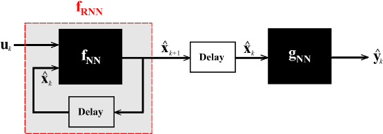
Figure 1: SSNN Block diagram.

This motivates the proposed state-space neural network with ordered variance (SSNNO) in which we present the idea of ordering the state variables so that the model order can be efficiently determined. To the best of the authors’ knowledge, this is the first work that incorporates the ordering of state variables in SSNN and presents a systematic way of determining the model order. The proposed SSNNO is inspired by the idea of ordering by variance introduced in the previous work [37], which presented an autoencoder with ordered variance (AEO). The AEO identifies a nonlinear static model from the data in an unsupervised setting, whereas the proposed SSNNO identifies a nonlinear dynamic model in a supervised setting. Compared to the existing literature, the major contributions in this paper are highlighted below:

1. The proposed SSNNO identifies a state-space model from the input-output data for which the predicted state variables are ordered in decreasing variance.

2. A systematic way of identifying the order of the model to predict the output with sufficient accuracy is presented, which is extended for model order reduction. Further, theoretical results on the existence of SSNNO with arbitrarily small prediction error is discussed.

The rest of the paper is organized as follows. Section II briefly discusses the relevant concepts from SSNN. The proposed SSNNO approach is presented in Section III, which consists of the nonlinear system identification using SSNNO and the extension of SSNNO for model order reduction. Section IV illustrates the numerical implementation of SSNNO and the comparison of simulation results with SSNN. Conclusions and future directions are discussed in Section V.

Notations: Scalars are denoted by normal font ($A,a$), matrices and vectors using the bold font ($\textbf{A},\textbf{a}$), and sets by blackboard bold font ($\mathbb{A}$). The set $\mathbb{R}^{n}$ denotes the $n$ - dimensional Euclidean space, and the space of $m\times n$ real matrices is denoted by $\mathbb{R}^{m\times n}$. The sample mean vector and sample covariance matrix of the vector x are denoted by $\bar{\textbf{x}},\textbf{V}_{\textbf{x}},$ respectively. For a matrix $\textbf{A}\in\mathbb{R}^{m\times n},$ the notations $\textbf{A}{(i,:)}$ and $\textbf{A}{(:,j)}$ denotes the $i^{th}$ row and $j^{th}$ column, respectively. The Euclidean norm of vector $\textbf{x}\in\mathbb{R}^{n}$ is denoted by ${\parallel\textbf{x}\parallel}$ and ${\parallel\textbf{A}\parallel}_{F}$ denotes the Frobenious norm of the matrix $\textbf{A}\in\mathbb{R}^{m\times n},$ where ${\parallel\textbf{x}\parallel}=\sqrt{\sum_{i=1}^{n}x_{i}^{2}}$ and ${\parallel\textbf{A}\parallel}_{F}=\sqrt{\sum_{i=1}^{m}\sum_{j=1}^{n}a_{ij}^{2}}=\sqrt{Trace(\textbf{A}^{T}\textbf{A})}.$ Finally, $\textbf{I}_{n}$ represents the identity matrix of size $n\times n,$ and 0 denotes the zero matrix of appropriate dimension.

2 Preliminaries

2.1 State-space Neural Network (SSNN)

Consider the discrete-time nonlinear system:

$$\textbf{x}_{k+1} =\textbf{f}(\textbf{x}_{k},\textbf{u}_{k})$$ (1)

$$\textbf{y}_{k} =\textbf{g}(\textbf{x}_{k})$$

where $\textbf{x}_{k}\in\mathbb{X}\subset\mathbb{R}^{n}$ is the state vector, $\textbf{u}_{k}\in\mathbb{U}\subset\mathbb{R}^{m}$ is the control input vector, $\textbf{y}_{k}\in\mathbb{Y}\subset\mathbb{R}^{p}$ is the output vector, $\mathbb{X},\mathbb{U},\mathbb{Y}$ are compact sets, $\textbf{f}:\mathbb{X}\times\mathbb{U}\rightarrow\mathbb{X}$ is the state function, and $\textbf{g}:\mathbb{X}\rightarrow\mathbb{Y}$ is the output function. Here, the output function is considered as a function of $\textbf{x}_{k}$ alone, i.e., we assume there is no direct feedforward term from the input to the output. The order of the system is denoted as $n$, which is the dimension of the state vector. The available information contains the input and output data:

$$\textbf{U}=\left[\begin{matrix}\textbf{u}_{1}&\textbf{u}_{2}&\dots&\textbf{u}_{N}\end{matrix}\right]$$ (2)

$$\textbf{Y}=\left[\begin{matrix}\textbf{y}_{1}&\textbf{y}_{2}&\dots&\textbf{y}_{N}\end{matrix}\right]$$

where $\textbf{u}_{k}$ and $\textbf{y}_{k},$ $k=1,\dots,N$ are the input and output samples at $N$ time instants. Each input sample $\textbf{u}_{k}$ contains $m$ input (control or manipulated) variables and each output sample $\textbf{y}_{k}$ consists of measurements of $p$ output (controlled) variables.

In SSNN, the objective is to fit the given input-output data with a state-space model. This is achieved in SSNN by representing the state and output functions using NNs [19]:

$$\hat{\textbf{x}}_{k+1} =\textbf{f}_{\text{NN}}(\hat{\textbf{x}}_{k},\textbf{u}_{k};\textbf{A}_{\textbf{f}})=\textbf{f}_{\text{NN}}(\hat{\textbf{x}}_{k},\textbf{u}_{k})$$ (3)

$$\hat{\textbf{y}}_{k} =\textbf{g}_{\text{NN}}(\hat{\textbf{x}}_{k};\textbf{A}_{\textbf{g}})=\textbf{g}_{\text{NN}}(\hat{\textbf{x}}_{k})$$

where $\hat{\textbf{x}}_{k}\in\mathbb{R}^{n}$ is the state vector predicted using SSNN, $\hat{\textbf{y}}_{k}\in\mathbb{R}^{p}$ is the predicted output, $\textbf{f}_{\text{NN}}:\mathbb{R}^{n}\times\mathbb{R}^{m}\rightarrow\mathbb{R}^{n},$ $\textbf{g}_{\text{NN}}:\mathbb{R}^{n}\rightarrow\mathbb{R}^{p}$ are the state and output NNs, and $\textbf{A}_{\textbf{f}}\in\mathbb{R}^{n_{f}},$ $\textbf{A}_{\textbf{g}}\in\mathbb{R}^{n_{g}}$ contains the weights and biases of state and output NNs, respectively. Generally, in SSNN, the order of the model is chosen the same as the system order, which is assumed to be known [29, 30, 31, 32]. The block diagram for SSNN is given in Fig. 1 in which $\textbf{f}_{\text{NN}}$ and $\textbf{g}_{\text{NN}}$ are feedforward NNs. The $\textbf{f}_{\textbf{NN}}$ with a feedback connection as in Fig. 1 becomes an RNN which is denoted as $\textbf{f}_{\text{RNN}}.$ The delay block stores and shifts the predicted state sample by one instant. In general, the state and output NNs can be represented as composite functions of the form:

$$\textbf{f}_{\text{NN}}=\textbf{f}_{L}(\dots\textbf{f}_{2}(\textbf{f}_{1}(\hat{\textbf{x}}_{k},\textbf{u}_{k})))$$ (4)

$$\textbf{g}_{\text{NN}}=\textbf{g}_{M}(\dots\textbf{g}_{2}(\textbf{g}_{1}(\hat{\textbf{x}}_{k})))$$

where $L$ and $M$ are the number of layers in state and output NNs, respectively. Here $\textbf{f}_{1},\dots,\textbf{f}_{L-1}$ are the hidden layers of the state NN and $\textbf{f}_{L}$ is the output layer. Let $\textbf{v}_{i}$ denote the input to the $i^{th}$ layer of state NN. Then, each layer of $\textbf{f}_{\text{NN}}$ can be represented as:

$$\textbf{f}_{i}(\textbf{v}_{i})=\bm{\sigma}_{\textbf{f}_{i}}(\textbf{A}_{\textbf{f}_{i}}\textbf{v}_{i}+\textbf{b}_{\textbf{f}_{i}})$$ (5)

where each element of $\textbf{f}_{i}$ represents a neuron in the $i^{th}$ layer of the state NN, $\bm{\sigma}_{\textbf{f}_{i}}=\left[\begin{matrix}\sigma_{1}\\ \vdots\\ \sigma_{n_{i}}\end{matrix}\right]$ contains the activation functions for each neuron in the $i^{th}$ layer, $n_{i}$ is the number of neurons in $i^{th}$ layer, $\textbf{A}_{\textbf{f}_{i}}\in\mathbb{R}^{n_{i}\times n_{i-1}}$ is the weight matrix, $\textbf{b}_{\textbf{f}_{i}}\in\mathbb{R}^{n_{i}}$ is the bias vector, $\textbf{v}_{i}\in\mathbb{R}^{n_{i-1}},$ $i=1,2,\dots,L$, $n_{0}=n+m,n_{L}=n,$ $\textbf{v}_{1}=\left[\begin{matrix}\hat{\textbf{x}}_{k}\\ \textbf{u}_{k}\end{matrix}\right]$ $,\hat{\textbf{x}}_{k+1}=\textbf{f}_{L}(\textbf{v}_{L})$.

Similarly, $\textbf{g}_{1},\dots,\textbf{g}_{M-1}$ represents the hidden layers of the output NN and $\textbf{g}_{M}$ is the output layer. Let $\textbf{z}_{i}$ denote the input to the $i^{th}$ layer of the output NN. Then, the layers of $\textbf{g}_{\text{NN}}$ can be represented as:

$$\textbf{g}_{i}(\textbf{z}_{i})=\bm{\sigma}_{\textbf{g}_{i}}(\textbf{A}_{\textbf{g}_{i}}\textbf{z}_{i}+\textbf{b}_{\textbf{g}_{i}})$$ (6)

where each element of $\textbf{g}_{i}$ represents a neuron in the $i^{th}$ layer of the output NN, $\bm{\sigma}_{\textbf{g}_{i}}=\left[\begin{matrix}\sigma_{1}\\ \vdots\\ \sigma_{p_{i}}\end{matrix}\right]$ contains the activation functions for each neuron in the $i^{th}$ layer, $p_{i}$ is the number of neurons in $i^{th}$ layer, $\textbf{A}_{\textbf{g}_{i}}\in\mathbb{R}^{p_{i}\times p_{{i-1}}}$ is the weight matrix, $\textbf{b}_{\textbf{g}_{i}}\in\mathbb{R}^{p_{i}}$ is the bias vector, $\textbf{z}_{i}\in\mathbb{R}^{p_{{i-1}}},$ $i=1,2,\dots,M$, $p_{0}=n,p_{M}=p,$ $\textbf{z}_{1}=\hat{\textbf{x}}_{k},$ $\hat{\textbf{y}}_{k}=\textbf{g}_{M}(\textbf{z}_{M})$.

Define the predicted state and output sequence using SSNN as:

$$\hat{\textbf{X}}=\left[\begin{matrix}\hat{\textbf{x}}_{1}&\hat{\textbf{x}}_{2}&\dots&\hat{\textbf{x}}_{N}\end{matrix}\right]$$ (7)

$$\hat{\textbf{Y}}=\left[\begin{matrix}\hat{\textbf{y}}_{1}&\hat{\textbf{y}}_{2}&\dots&\hat{\textbf{y}}_{N}\end{matrix}\right].$$

The predicted state sequence $\hat{\textbf{X}}=\textbf{f}_{\text{NN}}(\hat{\textbf{x}}_{1},\textbf{U})$ can be computed given the initial state and control sequence, by unfolding $\textbf{f}_{\text{RNN}}$ in time [38]:

$$\hat{\textbf{X}}=\left[\begin{matrix}\hat{\textbf{x}}_{1}&\textbf{f}_{\text{NN}}(\hat{\textbf{x}}_{1},\textbf{u}_{1})&\textbf{f}_{\text{NN}}\big{(}\textbf{f}_{\text{NN}}(\hat{\textbf{x}}_{1},\textbf{u}_{1}),\textbf{u}_{2}\big{)}&\dots&\textbf{f}_{\text{NN}}\big{(}\dots\textbf{f}_{\text{NN}}(\hat{\textbf{x}}_{1},\textbf{u}_{1}),\textbf{u}_{N-1}\big{)}\end{matrix}\right].$$ (8)

From this, the predicted output sequence $\hat{\textbf{Y}}=\textbf{g}_{\text{NN}}(\hat{\textbf{X}})$ is computed as

$$\hat{\textbf{Y}}=\left[\begin{matrix}\textbf{g}_{\text{NN}}(\hat{\textbf{x}}_{1})&\textbf{g}_{\text{NN}}(\hat{\textbf{x}}_{2})&\dots&\textbf{g}_{\text{NN}}(\hat{\textbf{x}}_{N})\end{matrix}\right].$$ (9)

The prediction performance of the SSNN is characterized by the output prediction error defined as:

$$J_{y}={\parallel\textbf{Y}-\hat{\textbf{Y}}\parallel}_{F}^{2}={\parallel\textbf{Y}-\textbf{g}_{\text{NN}}(\hat{\textbf{X}})\parallel}_{F}^{2}$$ (10)

which is also chosen as the loss function of SSNN. Define $\textbf{A}\in\mathbb{R}^{{n_{f}}+{n_{g}}}$ which contains the weights and biases for $\textbf{f}_{\text{NN}}$ and $\textbf{g}_{\text{NN}}$:

$$\textbf{A}=\left[\begin{matrix}\textbf{A}_{\textbf{f}}\\ \textbf{A}_{\textbf{g}}\end{matrix}\right].$$ (11)

The optimization problem for SSNN becomes:

$$\underset{\textbf{A}}{\min}\hskip 5.69046ptJ_{y}$$ (12)

which can be solved using backpropagation through time (BPTT) [6, 38] and truncated BPTT [39] algorithms.

The SSNN can learn nonlinear higher-order systems by increasing the number of neurons in the state and output NNs. As per UATs [24, 25], any continuous nonlinear function can be approximated with arbitrary accuracy by an NN with one hidden layer and an arbitrary number of neurons per layer. Similar results are also introduced for deep NNs with a bounded number of neurons per layer [26, 27]. This supports the approximation capabilities of NNs, thereby SSNNs. The theoretical results on the approximation capabilities of SSNNs are briefly discussed next.

Assumption 1 ([29]).

The state function $\textbf{f}:\mathbb{X}\times\mathbb{U}\rightarrow\mathbb{X}$ and output function $\textbf{g}:\mathbb{X}\rightarrow\mathbb{Y}$ in Eq. (1) are uniformly Lipschitz in x with $0<L_{f}<\infty$ and $0<L_{g}<\infty$ as the Lipschitz constants satisfying:

$${\parallel\textbf{f}(\textbf{x}_{1},\textbf{u})-\textbf{f}(\textbf{x}_{2},\textbf{u})\parallel}\leq L_{f}{\parallel\textbf{x}_{1}-\textbf{x}_{2}\parallel}$$ (13)

$${\parallel\textbf{g}(\textbf{x}_{1})-\textbf{g}(\textbf{x}_{2})\parallel}\leq L_{g}{\parallel\textbf{x}_{1}-\textbf{x}_{2}\parallel}$$

for all $\textbf{x}_{1},\textbf{x}_{2}\in\mathbb{X}$ and any $\textbf{u}\in\mathbb{U}$.

Lemma 1 ([29]).

Under Assumption 1, for any $\epsilon>0$ there exists an SSNN as in Eq. (3) with an appropriate initial condition $\hat{\textbf{x}}_{1}$ such that the output prediction error over any finite $N$ is bounded as:

$$J_{y}\leq\epsilon$$ (14)

for any nonlinear system (1) with bounded inputs.

Proof.

The UATs [24, 25, 26, 27] ensures that for any $\epsilon_{x}>0$ and $\epsilon_{y}>0,$ there exists $\textbf{f}_{\text{NN}}$ and $\textbf{g}_{\text{NN}}$ such that

$${\parallel\textbf{f}(\textbf{x},\textbf{u})-\textbf{f}_{\text{NN}}(\textbf{x},\textbf{u})\parallel}\leq\epsilon_{x}$$ (15)

$${\parallel\textbf{g}(\textbf{x})-\textbf{g}_{\text{NN}}(\textbf{x})\parallel}\leq\epsilon_{y}$$

for all $\textbf{x}\in\mathbb{X}$ and $\textbf{u}\in\mathbb{U}.$ Using this and the Lipschitz inequality in Eq. (13), the output error at $k^{th}$ instant can be bounded as:

$${\parallel\textbf{y}_{k}-\hat{\textbf{y}}_{k}\parallel} ={\parallel\textbf{g}(\textbf{x}_{k})-\textbf{g}_{\text{NN}}(\hat{\textbf{x}}_{k})\parallel}$$ (16)

$$={\parallel\textbf{g}(\textbf{x}_{k})-\textbf{g}(\hat{\textbf{x}}_{k})+\textbf{g}(\hat{\textbf{x}}_{k})-\textbf{g}_{\text{NN}}(\hat{\textbf{x}}_{k})\parallel}$$

$$\leq L_{g}{\parallel\textbf{x}_{k}-\hat{\textbf{x}}_{k}\parallel}+\epsilon_{y}.$$

Further, the state error term in the above equation can be bounded as:

$${\parallel\textbf{x}_{k}-\hat{\textbf{x}}_{k}\parallel} ={\parallel\textbf{f}(\textbf{x}_{k-1},\textbf{u}_{k-1})-\textbf{f}_{\text{NN}}(\hat{\textbf{x}}_{k-1},\textbf{u}_{k-1})\parallel}$$ (17)

$$={\parallel\textbf{f}(\textbf{x}_{k-1},\textbf{u}_{k-1})-\textbf{f}(\hat{\textbf{x}}_{k-1},\textbf{u}_{k-1})+\textbf{f}(\hat{\textbf{x}}_{k-1},\textbf{u}_{k-1})-\textbf{f}_{\text{NN}}(\hat{\textbf{x}}_{k-1},\textbf{u}_{k-1})\parallel}$$

$$\leq L_{f}{\parallel\textbf{x}_{k-1}-\hat{\textbf{x}}_{k-1}\parallel}+\epsilon_{x}$$

$$\leq L_{f}^{k}{\parallel\textbf{x}_{1}-\hat{\textbf{x}}_{1}\parallel}+(L_{f}^{k-1}+\dots+L_{f}+1)\epsilon_{x}$$

$$\leq M_{k}\epsilon_{x}$$

where $M_{k}=\sum_{i=0}^{k}L_{f}$ given that the initial state estimate satisfies ${\parallel\textbf{x}_{1}-\hat{\textbf{x}}_{1}\parallel}\leq\epsilon_{x}.$ Substituting Eq. (17) in (16) results in:

$${\parallel\textbf{y}_{k}-\hat{\textbf{y}}_{k}\parallel}\leq L_{g}M_{k}\epsilon_{x}+\epsilon_{y}.$$ (18)

Now, selecting $\epsilon_{x}=\frac{\epsilon}{2L_{g}M_{k}N}$ and $\epsilon_{y}=\frac{\epsilon}{2N}$ gives ${\parallel\textbf{y}_{k}-\hat{\textbf{y}}_{k}\parallel}\leq\frac{\epsilon}{N},$ which results in $J_{y}\leq\epsilon.$ ∎

In practice, the number of state variables and the initial state vector are unknown, especially for systems without a first principle model. Consequently, the main challenges of SSNN are selecting the number of state variables and neurons per layer for approximating a given input-output data. This is mostly done as a trial-and-error procedure, which requires considerable training and testing. Therefore, the main objective of this paper is to identify a state-space model and the order of the model systematically. In the next section, we present the SSNNO which can achieve the above objective.

3 State-space Neural Network with Ordered Variance (SSNNO)

The SSNNO introduces the idea of ordering in the state space where the state variables are ordered in terms of their variance. The ordering in variance is used to find a state-space model of minimum order that can fit the given input-output data. The state and output equations of SSNNO are represented as:

$$\textbf{x}_{\textbf{o}_{k+1}} =\textbf{f}_{\text{NNO}}(\textbf{x}_{\textbf{o}_{k}},\textbf{u}_{k},\textbf{A}_{\textbf{fo}})=\textbf{f}_{\text{NNO}}(\textbf{x}_{\textbf{o}_{k}},\textbf{u}_{k})$$ (19)

$$\hat{\textbf{y}}_{\textbf{o}_{k}} =\textbf{g}_{\text{NNO}}(\textbf{x}_{\textbf{o}_{k}},\textbf{A}_{\textbf{go}})=\textbf{g}_{\text{NNO}}(\textbf{x}_{\textbf{o}_{k}})$$

where $\textbf{x}_{\textbf{o}_{k}}\in\mathbb{R}^{l}$ is the state vector predicted using SSNNO and we assume $l\geq n$, $\hat{\textbf{y}}_{\textbf{o}_{k}}\in\mathbb{R}^{p}$ is the predicted output, $\textbf{f}_{\text{NNO}}:\mathbb{R}^{l}\times\mathbb{R}^{m}\rightarrow\mathbb{R}^{l},$ $\textbf{g}_{\text{NNO}}:\mathbb{R}^{l}\rightarrow\mathbb{R}^{p}$ are the state and output NNs, and $\textbf{A}_{\textbf{fo}}\in\mathbb{R}^{n_{fo}},$ $\textbf{A}_{\textbf{go}}\in\mathbb{R}^{n_{go}}$ contains the weights and biases of state and output NNs, respectively. In the proposed SSNNO, the state and output NNs are represented as:

$$\textbf{f}_{\text{NNO}}=\textbf{f}_{\textbf{o}_{L}}(\dots\textbf{f}_{\textbf{o}_{2}}(\textbf{f}_{\textbf{o}_{1}}(\textbf{x}_{\textbf{o}_{k}},\textbf{u}_{k})))$$ (20)

$$\textbf{g}_{\text{NNO}}=\textbf{g}_{\textbf{o}_{M}}(\dots\textbf{g}_{\textbf{o}_{2}}(\textbf{g}_{\textbf{o}_{1}}(\textbf{x}_{\textbf{o}_{k}})))$$

where $L$ and $M$ are the number of layers in state and output NNs. Here $\textbf{f}_{\textbf{o}_{i}},$ $i=1,\dots,L$ are the layers of the $\textbf{f}_{\text{NNO}}$ which are represented as:

$$\textbf{f}_{\textbf{o}_{i}}(\textbf{v}_{\textbf{o}_{i}})=\bm{\sigma}_{\textbf{fo}_{i}}(\textbf{A}_{\textbf{fo}_{i}}\textbf{v}_{\textbf{o}_{i}}+\textbf{b}_{\textbf{fo}_{i}})$$ (21)

where $\bm{\sigma}_{\textbf{fo}_{i}}=\left[\begin{matrix}\sigma_{1}\\ \vdots\\ \sigma_{n_{o_{i}}}\end{matrix}\right]$ contains the activation functions for each neuron in the $i^{th}$ layer, $n_{o_{i}}$ is the number of neurons in $i^{th}$ layer, $\textbf{A}_{\textbf{fo}_{i}}\in\mathbb{R}^{n_{o_{i}}\times n_{o_{i-1}}}$ is the weight matrix, $\textbf{b}_{\textbf{fo}_{i}}\in\mathbb{R}^{n_{o_{i}}}$ is the bias, $\textbf{v}_{\textbf{o}_{i}}\in\mathbb{R}^{n_{o_{i-1}}},$ $i=1,2,\dots,L$, $n_{o_{0}}=l+m,n_{o_{L}}=l,$ $\textbf{v}_{\textbf{o}_{1}}=\left[\begin{matrix}\textbf{x}_{\textbf{o}_{k}}\\ \textbf{u}_{k}\end{matrix}\right]$ $,\textbf{x}_{\textbf{o}_{k+1}}=\textbf{f}_{\textbf{o}_{L}}(\textbf{v}_{\textbf{o}_{L}})$.

Similarly, $\textbf{g}_{\textbf{o}_{i}},$ $i=1,\dots,M$ are the layers of $\textbf{g}_{\text{NNO}}$ which are represented as:

$$\textbf{g}_{\textbf{o}_{i}}(\textbf{z}_{\textbf{o}_{i}})=\bm{\sigma}_{\textbf{go}_{i}}(\textbf{A}_{\textbf{go}_{i}}\textbf{z}_{\textbf{o}_{i}}+\textbf{b}_{\textbf{go}_{i}})$$ (22)

where $\bm{\sigma}_{\textbf{go}_{i}}=\left[\begin{matrix}\sigma_{1}\\ \vdots\\ \sigma_{p_{o_{i}}}\end{matrix}\right]$ contains the activation functions for each neuron in the $i^{th}$ layer, $p_{o_{i}}$ is the number of neurons in $i^{th}$ layer, $\textbf{A}_{\textbf{go}_{i}}\in\mathbb{R}^{p_{o_{i}}\times p_{o_{i-1}}}$ is the weight matrix, $\textbf{b}_{\textbf{go}_{i}}\in\mathbb{R}^{p_{o_{i}}}$ is the bias, $\textbf{z}_{\textbf{o}_{i}}\in\mathbb{R}^{p_{o_{i-1}}},$ $i=1,2,\dots,M$, $p_{o_{0}}=l,p_{o_{M}}=p,$ $\textbf{z}_{\textbf{o}_{1}}=\textbf{x}_{\textbf{o}_{k}}$ $,\hat{\textbf{y}}_{\textbf{o}_{k}}=\textbf{g}_{\textbf{o}_{M}}(\textbf{z}_{\textbf{o}_{M}})$.

Define the predicted state and output data using SSNNO as:

$$\textbf{X}_{\textbf{o}}=\left[\begin{matrix}\textbf{x}_{\textbf{o}_{1}}&\textbf{x}_{\textbf{o}_{2}}&\dots&\textbf{x}_{\textbf{o}_{N}}\end{matrix}\right]$$ (23)

$$\hat{\textbf{Y}}_{o}=\left[\begin{matrix}\hat{\textbf{y}}_{\textbf{o}_{1}}&\hat{\textbf{y}}_{\textbf{o}_{2}}&\dots&\hat{\textbf{y}}_{\textbf{o}_{N}}\end{matrix}\right].$$

The output prediction error for SSNNO is defined as:

$$J_{yo}={\parallel\textbf{Y}-\hat{\textbf{Y}}_{o}\parallel}_{F}^{2}.$$ (24)

The loss function for SSNNO is defined as:

$$J_{o}= \underbrace{\alpha{\parallel\textbf{Y}-\textbf{g}_{\text{NNO}}(\textbf{X}_{\textbf{o}})\parallel}_{F}^{2}}_{J_{1}}+\underbrace{\beta{\parallel\textbf{Q}^{\frac{1}{2}}[\textbf{X}_{\textbf{o}}-\bar{\textbf{X}}_{\textbf{o}}]\parallel}_{F}^{2}}_{J_{2}}+\underbrace{\gamma{\parallel\textbf{A}_{\textbf{fo}}\parallel}_{F}^{2}+\lambda{\parallel\textbf{A}_{\textbf{go}}\parallel}_{F}^{2}}_{J_{3}}$$ (25)

where $\bar{\textbf{X}}_{\textbf{o}}=\left[\begin{matrix}\bar{\textbf{x}}_{\textbf{o}}&\bar{\textbf{x}}_{\textbf{o}}&\dots&\bar{\textbf{x}}_{\textbf{o}}\end{matrix}\right]\in\mathbb{R}^{l\times N}$ contains the mean predicted state $\bar{\textbf{x}}_{\textbf{o}}$ as its elements, $\alpha,\beta,\gamma,\lambda>0$ are the tuning parameters, and $\textbf{Q}=diag(q_{1},q_{2},\dots,q_{l})$ is the weighting matrix. The elements of Q are chosen as $0\leq q_{1}<q_{2}<\dots<q_{l}<\infty$ so that the state variables can be ordered in terms of decreasing variance [37]. Define the sample covariance matrix for the predicted state as:

$$\textbf{V}_{\textbf{x}_{\textbf{o}}}=\frac{1}{N-1}([\textbf{X}_{\textbf{o}}-\bar{\textbf{X}}_{\textbf{o}}][\textbf{X}_{\textbf{o}}-\bar{\textbf{X}}_{\textbf{o}}]^{T})$$ (26)

and the diagonal elements of $\textbf{V}_{\textbf{x}_{\textbf{o}}}$ gives the variances of the predicted state variables: $V_{{x_{\text{o}}}_{i}}=\textbf{V}_{{\textbf{x}_{\textbf{o}}}_{ii}},i=1,2,\dots,l.$ The loss function in Eq. (25) consists of three terms:

1. Output error term $J_{1}$: denotes the sum of square error between the given output and predicted output. Comparing $J_{1}$ with Eq. (24) gives $J_{yo}=\frac{1}{\alpha}J_{1}.$

2. State variance term $J_{2}$: used for ordering the state variables in terms of their variances:

   $$J_{2}=\beta\hskip 2.84544ptTrace([\textbf{X}_{\textbf{o}}-\bar{\textbf{X}}_{\textbf{o}}]^{T}\textbf{Q}[\textbf{X}_{\textbf{o}}-\bar{\textbf{X}}_{\textbf{o}}])=\beta(N-1)(q_{1}V_{x_{{\text{o}}_{1}}}+\dots+q_{l}V_{x_{{\text{o}}_{l}}})$$ (27)

   which indicates that by adjusting $q_{i}$ suitably the state variables can be ordered in decreasing variance.

3. Weight regularization term $J_{3}$: is used for avoiding overfitting and large weights, especially in the output NN.

Define $\textbf{A}_{\textbf{o}}\in\mathbb{R}^{{n_{fo}}+{n_{go}}+l}$ which contains the weights and biases for $\textbf{f}_{\text{NNO}},$ $\textbf{g}_{\text{NNO}}$ and the estimation of the initial state vector $\textbf{x}_{\textbf{o}_{1}}:$

$$\textbf{A}_{\textbf{o}}=\left[\begin{matrix}\textbf{A}_{\textbf{fo}}\\ \textbf{A}_{\textbf{go}}\\ \textbf{x}_{\textbf{o}_{1}}\end{matrix}\right].$$ (28)

The optimization problem for SSNNO becomes:

$$\underset{\textbf{A}_{\textbf{o}}}{\min}\hskip 5.69046ptJ_{o}.$$ (29)

Once the optimization problem is solved, the weights and biases in $\textbf{A}_{\textbf{o}}$ are used for constructing $\textbf{f}_{\text{NNO}}$ and $\textbf{g}_{\text{NNO}}$ which gives a state-space model of order $l$ as in Eq. (19). One of the advantages of SSNNO is its ability to identify a state-space model with a reduced order, which can predict the output with sufficient accuracy. This will be discussed in detail next.

3.1 System Identification and Model Order Reduction using SSNNO

This section discusses the effectiveness of SSNNO in identifying a nonlinear state-space model with reduced order. In SSNNO, the predicted state variables are ordered in terms of decreasing variance, which is achieved by adjusting the Q matrix in the state variance term in Eq. (27). This makes it easier to identify and separate state variables with zero or negligible variance. We denoted $l$ as the number of state variables in the SSNNO, which is also equal to the order of the trained model. Let $s$ be the order of the model (reduced-order) identified using SSNNO and $s\leq l$. To find $s,$ the number of state variables in SSNNO with significant variance is to be determined. This is achieved by defining a tolerance value $\delta\geq 0$, and identify the number of state variables in $\textbf{x}_{\textbf{o}}$ satisfying:

$$V_{{x_{\text{o}}}_{i}}>\delta$$ (30)

which gives $s.$ The variables with $V_{{x_{\text{\text{o}}}}_{i}}\leq\delta$ are called residual state variables for which the variance is considered to be negligible. Once $s$ is determined, a reduced order state-space model can be computed by setting $l=s$ and retraining SSNNO. However, this requires additional training and tuning of parameters. Therefore, in this paper, we focus on finding a reduced-order model directly from the trained model, i.e., without retraining. For that, after identifying $s,$ the elements in $\textbf{x}_{\textbf{o}},$ $\textbf{A}_{\textbf{fo}_{1}},$ $\textbf{A}_{\textbf{fo}_{L}},$ and $\textbf{A}_{\textbf{go}_{1}}$ are partitioned as follows:

$$\textbf{x}_{\textbf{o}}=\left[\begin{matrix}\textbf{x}_{s}\\ \textbf{x}_{r}\end{matrix}\right],\hskip 5.69046pt\textbf{A}_{\textbf{fo}_{1}}=\left[\begin{matrix}\textbf{A}_{\textbf{fo}_{1_{s}}}&\textbf{A}_{\textbf{fo}_{1_{r}}}&\textbf{A}_{\textbf{fo}_{1_{u}}}\end{matrix}\right]$$ (31)

$$\textbf{A}_{\textbf{fo}_{L}}=\left[\begin{matrix}\textbf{A}_{\textbf{fo}_{L_{s}}}\\ \textbf{A}_{\textbf{fo}_{L_{r}}}\end{matrix}\right],\hskip 5.69046pt\textbf{A}_{\textbf{go}_{1}}=\left[\begin{matrix}\textbf{A}_{\textbf{go}_{1_{s}}}&\textbf{A}_{\textbf{go}_{1_{r}}}\end{matrix}\right]$$

where $\textbf{x}_{s}\in\mathbb{R}^{s},\textbf{x}_{r}\in\mathbb{R}^{l-s},$ $\textbf{A}_{\textbf{fo}_{1_{s}}}\in\mathbb{R}^{n_{o_{1}}\times s},$ $\textbf{A}_{\textbf{fo}_{1_{r}}}\in\mathbb{R}^{n_{o_{1}}\times(l-s)},$ $\textbf{A}_{\textbf{fo}_{1_{u}}}\in\mathbb{R}^{n_{o_{1}}\times m},$ $\textbf{A}_{\textbf{fo}_{L_{s}}}\in\mathbb{R}^{s\times n_{o_{L-1}}},$ $\textbf{A}_{\textbf{fo}_{L_{r}}}\in\mathbb{R}^{(l-s)\times n_{o_{L-1}}},$ $\textbf{A}_{\textbf{go}_{1_{s}}}\in\mathbb{R}^{p_{o_{1}}\times s},$ and $\textbf{A}_{\textbf{go}_{1_{r}}}\in\mathbb{R}^{p_{o_{1}}\times(l-s)}.$ Further, the activation function for output layers of state and output NNs: $\bm{\sigma}_{\textbf{fo}_{L}}$ and $\bm{\sigma}_{\textbf{go}_{M}}$ are chosen as linear for which the bias terms are chosen as zero. Using this and Eq. (20), the state and output equations in Eq. (19) are rewritten as:

$$\textbf{x}_{\textbf{o}_{k+1}}= \left[\begin{matrix}\textbf{x}_{s_{k+1}}\\ \textbf{x}_{r_{k+1}}\end{matrix}\right]=\left[\begin{matrix}\textbf{A}_{\textbf{fo}_{L_{s}}}\\ \textbf{A}_{\textbf{fo}_{L_{r}}}\end{matrix}\right]\textbf{f}_{\textbf{o}_{L-1}}(\dots\textbf{f}_{\textbf{o}_{2}}(\bm{\sigma}_{\textbf{fo}_{1}}(\textbf{A}_{\textbf{fo}_{1_{s}}}\textbf{x}_{s_{k}}+\textbf{A}_{\textbf{fo}_{1_{r}}}\textbf{x}_{r_{k}}+\textbf{A}_{\textbf{fo}_{1_{u}}}\textbf{u}_{k}+\textbf{b}_{\textbf{fo}_{1}})))$$ (32)

$$\hat{\textbf{y}}_{\textbf{o}_{k}}= ~{}\textbf{g}_{\textbf{o}_{M}}(\dots\textbf{g}_{\textbf{o}_{2}}(\bm{\sigma}_{\textbf{go}_{1}}(\textbf{A}_{\textbf{go}_{1_{s}}}\textbf{x}_{s_{k}}+\textbf{A}_{\textbf{go}_{1_{r}}}\textbf{x}_{r_{k}}+\textbf{b}_{\textbf{go}_{1}}))).$$

We have $\textbf{V}_{\textbf{x}_{r}}$ is small which gives $\textbf{x}_{r_{k+1}}\approx\textbf{x}_{r_{k}}\approx\bar{\textbf{x}}_{r}.$ This simplifies Eq. (32) as:

$$\textbf{x}_{s_{k+1}} \approx\textbf{A}_{\textbf{fo}_{L_{s}}}\textbf{f}_{\textbf{o}_{L-1}}(\dots\textbf{f}_{\textbf{o}_{2}}(\bm{\sigma}_{\textbf{fo}_{1}}(\textbf{A}_{\textbf{fo}_{1_{s}}}\textbf{x}_{s_{k}}+\textbf{A}_{\textbf{fo}_{1_{u}}}\textbf{u}_{k}+\textbf{b}_{\textbf{fo}_{1_{s}}})))$$ (33)

$$\hat{\textbf{y}}_{s_{k}} =\textbf{g}_{\textbf{o}_{M}}(\dots\textbf{g}_{\textbf{o}_{2}}(\bm{\sigma}_{\textbf{go}_{1}}(\textbf{A}_{\textbf{go}_{1_{s}}}\textbf{x}_{s_{k}}+\textbf{b}_{\textbf{go}_{1_{s}}})))$$

where $\hat{\textbf{y}}_{s_{k}}\in\mathbb{R}^{p}$ is the output predicted using the reduced order model, $\textbf{b}_{\textbf{fo}_{1_{s}}}=\textbf{b}_{\textbf{fo}_{1}}+\textbf{A}_{\textbf{fo}_{1_{r}}}\bar{\textbf{x}}_{r},$ and $\textbf{b}_{\textbf{go}_{1_{s}}}=\textbf{b}_{\textbf{go}_{1}}+\textbf{A}_{\textbf{go}_{1_{r}}}\bar{\textbf{x}}_{r}$. By relabeling $\textbf{x}_{s_{k}}$ in Eq. (33) as $\textbf{x}_{\textbf{o}_{k}},$ a state-space model as in Eq. (19) is obtained for which $l=s$. Let $\hat{\textbf{Y}}_{s}$ denote the predicted output with the reduced order model over the training samples. Then the output prediction error using the reduced order model is defined as:

$$J_{ys}={\parallel\textbf{Y}-\hat{\textbf{Y}}_{s}\parallel}_{F}^{2}.$$ (34)

If the variance of the residual state variables is zero, then the output predicted by the reduced order model matches with the $\hat{\textbf{y}}_{\textbf{o}_{k}}.$ This leads to the following Lemma.

Lemma 2.

If $\textbf{V}_{\textbf{x}_{r}}=\textbf{0},$ then the reduced order model identified with SSNNO results in:

$$\hat{\textbf{y}}_{s_{k}}=\hat{\textbf{y}}_{\textbf{o}_{k}},\hskip 14.22636ptJ_{ys}=J_{yo}.$$ (35)

Proof.

$\textbf{V}_{\textbf{x}_{r}}=\textbf{0}$ gives $\textbf{x}_{r_{k}}=\bar{\textbf{x}}_{r}.$ Substituting this in $\hat{\textbf{y}}_{\textbf{o}_{k}}$ from Eq. (32) gives:

$$\hat{\textbf{y}}_{\textbf{o}_{k}} =\textbf{g}_{\textbf{o}_{M}}(\dots\textbf{g}_{\textbf{o}_{2}}(\bm{\sigma}_{\textbf{go}_{1}}(\textbf{A}_{\textbf{go}_{1_{s}}}\textbf{x}_{s_{k}}+\textbf{A}_{\textbf{go}_{1_{r}}}\textbf{x}_{r_{k}}+\textbf{b}_{\textbf{go}_{1}})))$$ (36)

$$=\textbf{g}_{\textbf{o}_{M}}(\dots\textbf{g}_{\textbf{o}_{2}}(\bm{\sigma}_{\textbf{go}_{1}}(\textbf{A}_{\textbf{go}_{1_{s}}}\textbf{x}_{s_{k}}+\textbf{A}_{\textbf{go}_{1_{r}}}\bar{\textbf{x}}_{r}+\textbf{b}_{\textbf{go}_{1}})))$$

$$=\textbf{g}_{\textbf{o}_{M}}(\dots\textbf{g}_{\textbf{o}_{2}}(\bm{\sigma}_{\textbf{go}_{1}}(\textbf{A}_{\textbf{go}_{1_{s}}}\textbf{x}_{s_{k}}+\textbf{b}_{\textbf{go}_{1_{s}}})))$$

$$=\hat{\textbf{y}}_{s_{k}}$$

which implies $\hat{\textbf{Y}}_{o}=\hat{\textbf{Y}}_{s}.$ Substituting $\hat{\textbf{Y}}_{o}$ instead of $\hat{\textbf{Y}}_{s}$ in Eq. (34) gives:

$$J_{ys}=J_{yo}.$$ (37)

This completes the proof. ∎

The algorithm for system identification using SSNNO is summarized below:

1:  Require $\textbf{U},$ Y

2:  Select $l,\delta$

3:  Select tuning parameters: $\alpha,\beta,\gamma,\lambda,\textbf{Q}$

4:  Initialize $\textbf{A}_{\textbf{o}}$

5:  Compute $\textbf{A}_{\textbf{o}}^{*}$ by solving the optimization problem in Eq. (29)

6:  Compute $\textbf{X}_{\textbf{o}}$ for the $\textbf{f}_{\text{NNO}}$ with parameters from $\textbf{A}_{\textbf{o}}^{*}$

7:  Compute $\textbf{V}_{\textbf{x}_{\textbf{o}}}$ using Eq. (26)

8:  for $i=l~{}to~{}1$ do

9:     if $V_{x_{\text{o}_{i}}}>\delta$ then

10:        $s=i$

11:        break

12:     end if

13:  end for

14:  Compute the state-space model of order $s$ as in Eq. (33).

Algorithm 1 SSNNO

3.2 Generality of SSNNO

As per Lemma 1, for a given $\epsilon$, there exists an SSNN with a finite number of parameters for which the output prediction error $J_{y}\leq\epsilon.$ In general, ordering can be achieved (without affecting the output prediction error) in a trained SSNN by relabeling the state variables in terms of their variances, i.e., the one with the highest variance is named as $x_{o_{1}},$ the next one $x_{o_{2}},$ and so on. This can be achieved by rearranging the columns/rows of the weights and biases of state and output NNs after training. This idea is used next to prove the existence of an SSNNO with arbitrarily small prediction error which leads to the following Lemma.

Lemma 3.

Under Assumption 1, for any $\epsilon>0,$ there exists an SSNNO as in Eq. (19) such that:

$$\textbf{V}_{\textbf{x}_{r}}=\textbf{0},\hskip 14.22636ptJ_{ys}=J_{yo}=J_{y}\leq\epsilon$$ (38)

for all $l\geq n$ and $n\leq s\leq l.$

Proof.

As per Lemma 1, for any $\epsilon>0$, there exists an SSNN for which $J_{y}\leq\epsilon.$ Next we construct an SSNNO from this SSNN which satisfies $J_{ys}=J_{yo}=J_{y}\leq\epsilon.$ The SSNNO is constructed from the SSNN in the following way:

1. The output layer in the state NN of SSNNO is constructed by rearranging the rows of output layer in SSNN in terms of state variable variances, i.e., let $\hat{x}_{j}$ has the $i^{th}$ largest variance in SSNN, then:

   1. for $i=1$ to $n$

      $$\textbf{A}_{\textbf{fo}_{L}}{(i,:)}=\textbf{A}_{\textbf{f}_{L}}{(j,:)}$$ (39)

   2. for $i=n+1$ to $l$

      $$\textbf{A}_{\textbf{fo}_{L}}{(i,:)}=\textbf{0}.$$ (40)

2. The first hidden layer in the state and output NNs of SSNNO is constructed by rearranging the columns of the corresponding layer in SSNN in terms of state variable variances, i.e., let $\hat{x}_{j}$ has the $i^{th}$ largest variance in SSNN, then:

   1. for $i=1$ to $n$

      $$\textbf{A}_{\textbf{fo}_{1}}{(:,i)}=\textbf{A}_{\textbf{f}_{1}}{(:,j)}$$ (41)

      $$\textbf{A}_{\textbf{go}_{1}}{(:,i)}=\textbf{A}_{\textbf{g}_{1}}{(:,j)}$$

   2. for $i=n+1$ to $l$

      $$\textbf{A}_{\textbf{fo}_{1}}{(:,i)}=\textbf{0}$$ (42)

      $$\textbf{A}_{\textbf{go}_{1}}{(:,i)}=\textbf{0}.$$

3. The layers 2 to $L-1$ in the state NN of SSNNO are chosen the same as in SSNN.

4. The layers 2 to $M$ in the output NN of SSNNO are chosen the same as in SSNN.

5. Finally, the initial state of SSNNO is constructed by rearranging the elements of the initial state in SSNN in terms of state variable variances, i.e., let $\hat{x}_{j}$ has the $i^{th}$ largest variance in SSNN, then:

   1. for $i=1$ to $n$

      $$x_{o_{1_{i}}}=\hat{x}_{{1_{j}}}$$ (43)

   2. for $i=n+1$ to $l$

      $$x_{o_{1_{i}}}=0.$$ (44)

In the constructed SSNNO with initial state , the first $n$ state variables are ordered in terms of decreasing variance, and the remaining $l-n$ state variables have zero mean and variance. Therefore, $\textbf{V}_{\textbf{x}_{r}}=\textbf{0}$ for all $s\geq n$ which gives $J_{ys}=J_{yo}$ (using Lemma 2). Further, the predicted output with constructed SSNNO results in:

$$\hat{\textbf{y}}_{\textbf{o}_{k}} =\textbf{g}_{\textbf{o}_{M}}(\dots\textbf{g}_{\textbf{o}_{2}}(\bm{\sigma}_{\textbf{go}_{1}}(\textbf{A}_{\textbf{go}_{1}}(:,1)x_{o_{k_{1}}}+...+\textbf{A}_{\textbf{go}_{1}}(:,n)x_{o_{k_{n}}}+\textbf{0}\hskip 1.42271ptx_{o_{k_{n+1}}}+\dots+\textbf{0}\hskip 1.42271ptx_{o_{k_{l}}})))$$ (45)

$$=\textbf{g}_{\textbf{o}_{M}}(\dots\textbf{g}_{\textbf{o}_{2}}(\bm{\sigma}_{\textbf{go}_{1}}(\textbf{A}_{\textbf{go}_{1}}(:,1)x_{o_{k_{1}}}+...+\textbf{A}_{\textbf{go}_{1}}(:,n)x_{o_{k_{n}}})))$$

$$=\textbf{g}_{M}(\dots\textbf{g}_{2}(\bm{\sigma}_{\textbf{g}_{1}}(\textbf{A}_{\textbf{g}_{1}}(:,1)\hat{x}_{{k}_{1}}+...+\textbf{A}_{\textbf{g}_{1}}(:,n)\hat{x}_{{k}_{n}})))$$

$$=\hat{\textbf{y}}_{k}$$

which implies $\hat{\textbf{Y}}_{o}=\hat{\textbf{Y}}.$ Substituting $\hat{\textbf{Y}}$ instead of $\hat{\textbf{Y}}_{o}$ in Eq. (24) gives:

$$J_{yo}=J_{y}.$$ (46)

This completes the proof. ∎

Remark 1.

The SSNNO has the following advantages over the SSNN:

1. Ordering of state variables: which leads to having a structure in the identified state-space in terms of the variance.

2. Identifying the order of the model: SSNNO gives a systematic way of identifying the order of the state-space model, whereas, in SSNN, the model-order identification is mostly a trial-and-error procedure. In real-world processes, the actual order of the system is unknown and difficult to estimate. This makes the SSNNO a suitable choice for system identification of large processes.

3. Flexibility in modeling: the state and output NNs in SSNNO can be deep-NNs with arbitrary width and depth. Further, the weight regularization term in SSNNO helps in controlling the magnitude of the model parameters and state variables.

Remark 2.

The shortcomings of SSNNO are:

1. Convergence: The optimization problem for SSNNO in Eq. (29) is a nonlinear programming problem and can be nonconvex. Therefore, convergence to a global optimal solution is not guaranteed, and the solution depends on the initial guess.

2. Stability: identifying a stable state-space model that fits the input-output data is not guaranteed. This issue could be resolved by incorporating LMI-based stability constraints [29] or Lyapunov inequalities in SSNNO, which is considered a possible future work.

Remark 3.

The proposed SSNNO has applications in the following areas:

1. Data-driven control: which uses mathematical models learned from data for designing control schemes [23, 40]. The SSNNO can be used for designing data-driven state feedback-based control schemes such as MPC, LQR, adaptive control, etc.

2. Model order reduction: is achieved when the identified order is lesser than the actual order of the system, i.e., $s<n$. This can occur if some of the state variables have fast transient behavior, which makes them almost static, i.e., they reach the steady state almost instantaneously, which makes their variances small.

3. State estimation: The model identified with SSNNO can be used for designing state estimators such as Kalman filters, moving horizon estimators, etc.

4. Fault detection and diagnosis: where the model can be used to detect or predict fault events in the process and identify their root causes.

4 Simulation Results

The proposed SSNNO is illustrated on a continuous stirred tank reactor (CSTR) system defined by the state equation in discrete time:

$$\textbf{x}_{k+1}=\textbf{x}_{k}+\int_{kT}^{(k+1)T}\textbf{f}_{c}(\textbf{x}(t),\textbf{u}(t))dt$$ (47)

where $T$ is the sampling period, $k$ is the discrete time instant, $t$ is the continuous time instant, $\textbf{f}_{c}$ is the state function of CSTR in continuous time:

$$\textbf{f}_{c}=\left[\begin{matrix}-x_{1}+D_{a}(1-x_{1})e^{x_{2}}\\ x_{2}+B\hskip 2.84544ptD_{a}(1-x_{1})e^{x_{2}}-D_{b}(x_{2}-u)\end{matrix}\right]$$ (48)

where $x_{1}$ is the reactant concentration, $x_{2}$ is the reactant temperature, and $B,D_{a},D_{b}$ are system parameters which are selected as $B=22.0,D_{a}=0.082,D_{b}=3.0.$ The temperature of the reactant is considered as the output, which results in:

$$y_{k}=x_{2_{k}}+v_{k}$$ (49)

where $v_{k}$ is the measurement noise, which is considered as Gaussian white noise. The input-output data is generated by a forward simulation of Eqs. (47)-(49) over $N_{s}=900$ instants with the sampling period $T=1\hskip 2.84544ptsec.,$ initial condition $\textbf{x}_{1}=\left[\begin{matrix}0\\ 0\end{matrix}\right]$ and the control input $u$ is chosen as a pseudorandom binary sequence (PRBS) signal.

The first 500 samples of the dataset are used for training the SSNNO and is denoted as $\textbf{U}_{tr},\textbf{Y}_{tr}$ while the remaining samples for testing which is denoted as $\textbf{U}_{ts},\textbf{Y}_{ts}$. The SSNNO is trained using the training data where the loss function is chosen as in Eq. (25) with $\textbf{U}=\textbf{U}_{tr},$ $\textbf{Y}=\textbf{Y}_{tr}$ and the activation function is chosen as hyperbolic tangent (tanh) function. The tuning parameters are chosen as $\alpha=0.3,\beta=0.1,\gamma=0,\lambda=0.1.$ The weighting matrix is chosen as $\textbf{Q}=diag(0.01,0.02,0.05)$ for $l=3,$ and $\textbf{Q}=diag(0.01,0.02,0.05,0.07)$ for $l=4.$ The unconstrained optimization problem in Eq. (29) is solved for $\textbf{A}_{\textbf{o}}$ using the Quasi-Newton method. Figs. 2 and 3 show the response with SSNNO with $l=3$ for CSTR without uncertainties and with white noise, respectively. The figures show the response (actual output v/s predicted output) for the training input, testing input, and step input, where it can be observed that the output predicted by SSNNO matches the actual output. Table I shows the variances of the state variables with SSNNO and SSNN (for which $\alpha=1,\beta=0,\gamma=0,\lambda=0$) for $l=3$. Here, we can observe that the variances are not ordered in SSNN and are nonzero for all three state variables. Whereas the variances with SSNNO are ordered, and the variance of the third state variable is zero. Further, Table I shows the mean square error between the given and predicted output for the training and testing data, denoted by $mse_{tr}$ and $mse_{ts},$ respectively. Similarly, Table II shows the variances of the state variables with SSNNO and SSNN for $l=4$, where SSNNO achieves ordering with the last two state variables having zero variances. From Tables I and II, it can be observed that the output prediction errors with SSNNO and SSNN are almost the same. The simulation results illustrate the effectiveness of SSNNO in ordering the state variables and, thereby, determining the dimension of the state vector. Selecting $\delta=0.0001$ gives the order of the model $s=2.$ Further, here we can observe that the variance of $x_{o_{2}}$ is nearly zero, which leads to the possibility of model order reduction. For example, selecting $\delta=0.3$ results in $s=1$ which gives a first-order model.

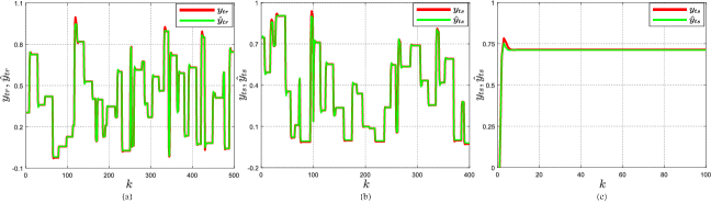
Figure 2: Response of SSNNO for CSTR without uncertainties: (a) Training (b) Testing (c) Step test.

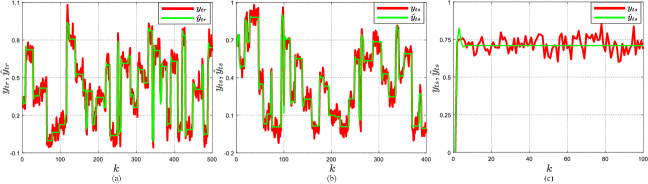
Figure 3: Response of SSNNO for CSTR with white noise: (a) Training (b) Testing (c) Step test.

Table 1: Performance comparison for third-order model.

Performance measure	SSNNO	SSNN
$V_{x_{\text{NN}_{1}}}$	0.1379	0.0029
$V_{x_{\text{NN}_{2}}}$	0.0002	0.0010
$V_{x_{\text{NN}_{3}}}$	0.0000	0.0264
$mse_{tr}$	0.0026	0.0026
$mse_{ts}$	0.0025	0.0025

Table 2: Performance comparison for fourth-order model.

Performance measure	SSNNO	SSNN
$V_{x_{\text{NN}_{1}}}$	0.1372	0.0263
$V_{x_{\text{NN}_{2}}}$	0.0002	0.0047
$V_{x_{\text{NN}_{3}}}$	0.0000	0.0446
$V_{x_{\text{NN}_{4}}}$	0.0000	0.0431
$mse_{tr}$	0.0026	0.0025
$mse_{ts}$	0.0046	0.0049

5 Conclusions

The paper presented a state-space neural network with ordered variance (SSNNO), which results in the identification of a state-space model where the state variables are ordered in terms of decreasing variance. Further, the approach also identifies the minimum order of the state-space model to predict the output with sufficient accuracy. The efficiency of the approach is illustrated using simulation on a CSTR system. Possible future works are the application of the approach in data-driven control and the analysis of the approach for theoretical guarantees on ordering, stability, etc.

References

- [1] L. Ljung, “System Identification: Theory for the User, Second Edition,” Prentice Hall, 1999.
- [2] S. Yin, H. Gao, and O. Kaynak, “Data-Driven Control and Process Monitoring for Industrial Applications—Part I ,” IEEE Transactions on Industrial Electronics, vol. 61, no. 11, pp. 6356 - 6359, Nov. 2014.
- [3] S. Billings, “Nonlinear System Identification: NARMAX Methods in the Time, Frequency, and Spatio-Temporal Domains,” John Wiley and Sons, 2013.
- [4] S. Bhartiya and J. Whiteley,“Factorized Approach to Nonlinear MPC Using a Radial Basis Function Model,” AIChE journal, vol. 26, pp. 1185-1199, Feb. 2001.
- [5] G. Pillonetto, F. Dinuzzo, T. Chen, G. Nicolao, and L. Ljung, “Kernel methods in system identification, machine learning, and function estimation: A survey,” Automatica, vol. 50, pp. 657-682, 2014.
- [6] K. Narendra and K. Parthasarathy, “Identification and control of dynamical systems using neural networks ,” IEEE Transactions on Neural Networks, vol. 1, no. 1, pp. 6356 - 6359, Mar. 1990.
- [7] A. Delgado, C. Karnbhampati, and K. Warwick, “Dynamic recurrent neural network for system identification and control ,” IEEE Proceedings of Control Theory Applications, vol. 142, pp. 307 - 314, Jul. 1995.
- [8] D. Liberzon, “Calculus of Variations and Optimal Control Theory: A Concise Introduction,” Princeton University Press, 2011.
- [9] F. Borrelli, A. Bemporad and M. Morari “Predictive Control for Linear and Hybrid Systems,” Cambridge University Press, 2017.
- [10] Y. Shtessel, C. Edwards, L. Fridman, A. Levant, “Sliding Mode Control and Observation,” Springer, 2014.
- [11] J. Paduart, L. Lauwers, J. Swevers, K. Smolders, J. Schoukens, and R. Pintelon , “Identification of nonlinear systems using polynomial nonlinear state space models,” Automatica, vol. 46, pp. 647–656, 2010.
- [12] P. Overschee , B. Moor, “Subspace Identification for Linear Systems: Theory — Implementation — Applications,” Kluwer Academic Publishers, 1996.
- [13] J. Noel and G. Kerschen, “Frequency-domain subspace identification for nonlinear mechanical systems,” Mechanical Systems and Signal Processing, vol. 40, pp. 701– 717, 2013.
- [14] L. Lee and K. Poolla, “Identification of Linear Parameter-Varying Systems Using Nonlinear Programming,” Journal of Dynamic Systems, Measurement, and Control, vol. 121, pp. 71 - 78, Mar. 1999.
- [15] M. Petreczky, R. Toth, G. Mercere, “Realization Theory for LPV State-Space Representations With Affine Dependence,” IEEE Transactions on Automatic Control, vol. 62, no. 9, pp. 4667 - 4674, Sep. 2017.
- [16] C. Verhoek, G. Beintema, S. Haesaert, M. Schoukens and R. Toth, “Deep-Learning-Based Identification of LPV Models for Nonlinear Systems,” IEEE 61st Conference on Decision and Control (CDC), pp. 3274-3280, Cancun, Mexico, Dec. 2022.
- [17] T. Schon, A. Wills, and B. Ninness, “System identification of nonlinear state-space models,” Automatica, vol. 47, pp. 39–49, 2011.
- [18] T. Schon, A. Svensson, L. Murray, and F. Lindsten, “Probabilistic learning of nonlinear dynamical systems using sequential Monte Carlo,” Mechanical Systems and Signal Processing, vol. 104, pp. 866– 883, 2018.
- [19] J. Suykens, B. Moor, and J. Vandewalle, “Nonlinear system identification using neural state space models, applicable to robust control design,” International Journal of Control, vol. 62, pp. 129–152, 1995.
- [20] J. Zamarreno, P. Vega, L. Garcia, M. Francisco, “State-space neural network for modelling, prediction, and control,” Control Engineering, vol. 8, pp. 1063-1075, 2000.
- [21] Q. Lu and V. Zavala, “Image-based model predictive control via dynamic mode decomposition,” arXiv, 2020.
- [22] D. Masti and A. Bemporad, “Learning nonlinear state-space models using deep autoencoders,” IEEE 61st Conference on Decision and Control (CDC), pp. 3862–3867, 2018.
- [23] D. Masti and A. Bemporad, “Learning nonlinear state–space models using autoencoders,” Automatica, vol. 129, pp. 1–9, 2021.
- [24] G. Cybenko,,“Approximation by Superpositions of a Sigmoidal function”, Mathematics of Control, Signals, and Systems, vol. 2, pp. 303-314, Dec. 1989.
- [25] K. Hornik, M. Stinchcombe, H. White, “Multilayer Feedforward Networks are Universal Approximators”, Neural Networks, vol. 2, pp. 359–366, Mar. 1989.
- [26] Z. Lu, H. Pu, F. Wang, Z. Hu, and L. Wang, “The Expressive Power of Neural Networks: A View from the Width”, Conference on Neural Information Processing Systems, Long Beach, CA, USA., 2017.
- [27] S. Park, C. Yun, J. Lee, and J. Shin, “Minimum Width for Universal Approximation”, International Conference on Learning Representations, Vienna, Austria, 2021.
- [28] J. Zamarreno and P. Vega, “State space neural network. Properties and application,” Neural Network, vol. 11, pp. 1099–1112, Mar. 1998.
- [29] K. Kim, E. Patrón, R. Braatz, “Standard representation and unified stability analysis for dynamic artificial neural network models,” Neural Networks, vol. 98, pp. 251–262, 2018.
- [30] M. Schoukens, “Improved Initialization of State-Space Artificial Neural Networks,” 2021 European Control Conference (ECC), pp. 1913-1918, Delft, Netherlands, Jun. 2021.
- [31] G. Beintema, R. Toth, and M. Schoukens, “Nonlinear state-space identification using deep encoder networks,” Proceedings of Machine Learning Research, vol. 144, pp. 1-10, 2021.
- [32] G. Beintema, R. Toth, and M. Schoukens, “Deep subspace encoders for nonlinear system identification,” Automatica, vol. 196, pp. 1-13, 2023.
- [33] F. Arnold and R. King, “State–space modeling for control based on physics-informed neural networks,” Engineering Applications of Artificial Intelligence, vol. 101, pp. 1-10, May 2021.
- [34] R, Patel, S. Bhartiya, and R. Gudi, “Optimal temperature trajectory for tubular reactor using physics informed neural networks,” Journal of Process Control, vol. 128, Aug. 2023.
- [35] R. Toth, C. Lyzell, M. Enqvist, P. Heuberger, and P. Hof, “Order and structural dependence selection of LPV-ARX models using a nonnegative garrote approach,” IEEE Conference on Decision and Control, Shanghai, China, Dec. 2009.
- [36] R. Toth, H. Hjalmarsson and C. Rojas, “Order and Structural Dependence Selection of LPV-ARX Models Revisited,” IEEE Conference on Decision and Control, Hawaii, USA, Dec. 2012.
- [37] M. Augustine, P. Patil, M. Bhushan, and S. Bhartiya,“Autoencoder with Ordered Variance for Nonlinear Model Identification,” arXiv, Feb. 2024.
- [38] P. Werbos,“Backpropagation through time: what it does and how to do it,” Proceedings of the IEEE, vol. 78, pp. 1550 - 1560, Oct. 1990.
- [39] R. Williams and D. Zipser, “Gradient-based learning algorithms for recurrent networks and their computational complexity ,” Backpropagation: Theory, Architectures, and Applications, pp. 1-45, 1995.
- [40] J. Berberich, J. Kohler, M. Muller, and F. Allgower, “Data-Driven Model Predictive Control With Stability and Robustness Guarantees ,” IEEE Transactions on Automatic Control, vol. 66, no. 4, pp. 1702-1717, Apr. 2021.