SigDiffusions: Score-Based Diffusion Models for
Long Time Series via Log-Signature Embeddings

Abstract

Score-based diffusion models have recently emerged as state-of-the-art generative models for a variety of data modalities. Nonetheless, it remains unclear how to adapt these models to generate long multivariate time series. Viewing a time series as the discretization of an underlying continuous process, we introduce SigDiffusion, a novel diffusion model operating on log-signature embeddings of the data. The forward and backward processes gradually perturb and denoise log-signatures preserving their algebraic structure. To recover a signal from its log-signature, we provide new closed-form inversion formulae expressing the coefficients obtained by expanding the signal in a given basis (e.g. Fourier or orthogonal polynomials) as explicit polynomial functions of the log-signature. Finally, we show that combining SigDiffusion with these inversion formulae results in highly realistic time series generation, competitive with the current state-of-the-art on various datasets of synthetic and real-world examples.

1 Introduction

Time series generation has been the focus of many research contributions in recent years due to the increasing demand for high-quality data augmentation in fields such as healthcare [64] and finance [30]. Because the sampling rate is often arbitrary and non-uniform, it is natural to assume that the data is collected from measurements of some underlying physical system that evolves in continuous time. This requires the adoption of modelling tools capable of processing temporal signals as continuous functions of time. We will often refer to such functions as paths.

The idea of representing a path via its iterated integrals has been the object of numerous mathematical studies, from geometry [12, 13] to control theory [24] to stochastic analysis [41]. The collection of such iterated integrals is often referred to as the signature of a path. Thanks to its numerous algebraic and analytic properties, which we will briefly summarise in Section 2, the signature provides a universal feature map for temporal signals evolving in continuous time, which is faithful, robust to irregular sampling, and efficient to compute. As a result, signature methods have recently become mainstream in many areas of machine learning dealing with irregular time series, from deep learning [36, 47, 15, 16] to kernel methods [57, 39, 32], with applications in quantitative finance [3, 58, 29, 48], cybersecurity [17], weather forecasting [38], and causal inference [45]. For a concise summary of this topic, we refer the interested reader to a recent survey [23].

Score-based diffusion models have recently become a mainstream tool for modelling complex distributions in computer vision, audio, and text [61, 5, 51, 7, 67]. The main idea consists of gradually perturbing the observed data distribution with noise following a reversible diffusion process trained via score-matching techniques. The forward diffusion is trained until attaining some base distribution which is easy to sample. A sample from the learned data distribution is then generated by running the backward denoising process starting from the base distribution.

Despite recent efforts summarised in Section 4, it remains unclear how to adapt score-based diffusion models to generate long signals in continuous time.

Contributions

In this paper, we make use of the log-signature, a compressed version of the signature, as a parameter-free Lie algebra embedding for time series. In Section 2, we introduce SigDiffusion, a new diffusion model that gradually perturbs and denoises log-signatures preserving their algebraic structure. To recover the underlying path from its log-signature embedding, we provide novel closed-form inversion formulae in Section 3. Notably, we prove that the coefficients in the expansion of a path in a given basis, such as Fourier or orthogonal polynomials, can be expressed as explicit polynomial functions on the log-signature. Our results provide a major improvement over existing signature inversion algorithms [22, 36, 10] which often suffer from scalability issues and, in general, are only effective on simple examples of short piecewise-linear paths. Finally, in Section 5, we demonstrate how the combination of SigDiffusion with our inversion formulae provides a highly realistic time series generative approach, competitive with state-of-the-art diffusion models for temporal data on various datasets of synthetic and real-world examples.

2 Generating log-signatures with score-based diffusion models

The definition of the log-signature requires an initial algebraic setup. We will limit ourselves to report only some key results needed for our approach. Additional details on signatures can be found in Appendix A. We begin this section by recalling the relevant background material before introducing our SigDiffusion model.

2.1 Algebraic setup

For any positive integer $n\in\mathbb{N}$ we consider the truncated tensor algebra over $\mathbb{R}^{d}$

$$T^{n}(\mathbb{R}^{d}):=\bigoplus_{k=0}^{n}(\mathbb{R}^{d})^{\otimes k},$$

where $\otimes$ denotes the outer product of vector spaces. For any scalar $\alpha\in\mathbb{R}$, we denote by $T^{n}_{\alpha}(\mathbb{R}^{d})=\{A\in T^{n}(\mathbb{R}^{d}):A_{0}=\alpha\}$ the hyperplane of elements in $T^{n}(\mathbb{R}^{d})$ with the $0^{th}$ term equal to $\alpha$.

$T^{n}(\mathbb{R}^{d})$ is a non-commutative algebra when endowed with the tensor product $\cdot$ defined for any two elements $A=\left(A_{0},A_{1},...,A_{n}\right)$ and $B=\left(B_{0},B_{1},...B_{n}\right)$ of $T^{n}(\mathbb{R}^{d})$ as follows

$$A\cdot B=\left(C_{0},C_{1},...,C_{n}\right)\in T^{n}(\mathbb{R}^{d}),\quad\text{ where }\quad C_{k}=\sum_{i=0}^{k}A_{i}\otimes B_{k-i}\in(\mathbb{R}^{d})^{\otimes k}.$$

The standard basis of $\mathbb{R}^{d}$ is denoted by $e_{1},e_{2},...,e_{d}$. We will refer to these basis elements as letters. Elements of the the induced standard basis of $T^{n}(\mathbb{R}^{d})$ are often referred to as words and abbreviated

$$e_{i_{1}i_{2}...i_{k}}=e_{1}\otimes e_{2}\otimes...\otimes e_{k},\quad\text{for}\quad 1\leq i_{1},...,i_{k}\leq d\text{ and }0\leq k\leq n.$$

We will make use of the dual pairing notation $\langle e_{i_{1}i_{2}...i_{k}},A\rangle\in\mathbb{R}$ to denote the $(i_{1},...,i_{k})^{th}$ element of a tensor $A\in T^{n}(\mathbb{R}^{d})$. This pairing is extended by linearity to any linear combination of words.

Following [55], the truncated tensor algebra $T^{n}(\mathbb{R}^{d})$ carries several additional algebraic structures.

Firstly, it is a Lie algebra, where the Lie bracket is the commutator

$$[A,B]=A\cdot B-B\cdot A\quad\text{for }A,B\in T^{n}(\mathbb{R}^{d}).$$

We denote by $\mathcal{L}^{n}(\mathbb{R}^{d})$ the smallest Lie subalgebra of $T^{n}(\mathbb{R}^{d})$ containing $\mathbb{R}^{d}$. We note that the Lie algebra $\mathcal{L}^{n}(\mathbb{R}^{d})$ is a vector space of dimension $\beta(d,n)$ with

$$\beta(d,n)=\sum_{k=1}^{n}\frac{1}{k}\sum_{i|k}\mu\left(\frac{k}{i}\right)d^{i},$$

where $\mu$ is the Möbius function [55]. Bases of this space are known as Hall bases [55, 53]. One of the most well-known bases is the Lyndon basis indexed by Lyndon words. A Lyndon word is a word occurring lexicographically earlier than any word obtained by cyclically rotating its elements.

Secondly, $T^{n}(\mathbb{R}^{d})$ is also a commutative algebra with respect to the shuffle product $\shuffle$. On basis elements, the shuffle product of two words of length $r$ and $s$ (with $r+s\leq n$) is the sum over the $r+s\choose s$ ways of interleaving the two words. For a more formal definition see [55, Section 1.4].

Related to the shuffle product is the right half-shuffle product $\succ$ defined recursively as follows: for any two words $e_{i_{1}...i_{r}}$ and $e_{j_{1}...j_{s}}$ and letter $e_{j}$

$$e_{i_{1}...i_{r}}\succ e_{j}=e_{i_{1}...i_{r}j}\quad\text{and}\quad e_{i_{1}...i_{r}}\succ e_{j_{1}...j_{s}}=(e_{i_{1}...i_{r}}\succ e_{j_{1}...j_{s-1}}+e_{j_{1}...j_{s-1}}\succ e_{i_{1}...i_{r}})\cdot e_{j_{s}}.$$

The right half-shuffle product will be useful for carrying out computations in the next section. Note that the following relation between shuffle and right half-shuffle products holds [59]

$$e_{i_{1}...i_{r}}\shuffle e_{j_{1}...j_{s}}=e_{i_{1}...i_{r}}\succ e_{j_{1}...j_{s}}+e_{j_{1}...j_{s}}\succ e_{i_{1}...i_{r}}.$$

Equipped with this algebraic setup, we can now introduce the signature.

2.2 The (log)signature

Let $x:[0,1]\to\mathbb{R}^{d}$ be a smooth path. The step-$n$ signature $S^{\leq n}(x)$ of $x$ is defined as the following collection of iterated integrals

$$S^{\leq n}(x)=\left(1,S_{1}(x),....S_{n}(x)\right)\in T_{1}^{n}(\mathbb{R}^{d})$$ (1)

where

$$S_{k}(x)=\int_{0\leq t_{1}<...<t_{k}\leq 1}dx_{t_{1}}\otimes...\otimes dx_{t_{k}}\in(\mathbb{R}^{d})^{\otimes k}\quad\text{for }1\leq k\leq n.$$

An important property of the signature is usually referred to as the shuffle identity. This result is originally due to Ree [52]. For a modern proof see [8, Theorem 1.3.10].

Theorem 2.1 (Shuffle identity).

Let $x:[0,1]\to\mathbb{R}^{d}$ be a smooth path. For any two words $e_{i_{1}...i_{r}}$ and $e_{j_{1}...j_{s}}$, with $0\leq r,s\leq n$, the following two identities hold

$$\left\langle e_{i_{1}...i_{r}}\shuffle e_{j_{1}...j_{s}},S^{\leq n}({x})\right\rangle=\left\langle e_{i_{1}...i_{r}},S^{\leq n}({x})\right\rangle\left\langle e_{j_{1}...j_{s}},S^{\leq n}({x})\right\rangle,$$

$$\left\langle e_{i_{1}...i_{r}}\succ e_{j_{1}...j_{s}},S^{\leq n}({x})\right\rangle=\int_{0}^{1}\left\langle e_{i_{1}...i_{r}},S^{\leq n}({x})_{t}\right\rangle d\left\langle e_{j_{1}...j_{s}},S^{\leq n}({x})_{t}\right\rangle,$$

where $S^{\leq n}(x)_{t}$ is the step-$n$ signature of the path $x$ restricted to the interval $[0,t]$.

An example of simple computations using the shuffle identity is presented in Appendix A.1.

Moreover, it turns out that the signature is more than just a generic element of $T_{1}^{n}(\mathbb{R}^{d})$; in fact, its range has the structure of a Lie group as we shall explain next. Recall that the tensor exponential $\exp$ and the tensor logarithm $\log$ are maps from $T^{n}(\mathbb{R}^{d})$ to itself defined as follows

$$\exp(A):=\sum_{k\geq 0}\frac{1}{k!}A^{\otimes k}\quad\text{and}\quad\log(\mathbf{1}+A)=\sum_{k\geq 1}\frac{(-1)^{k-1}}{k}(A)^{\otimes k}$$

where $\mathbf{1}=(1,0,...,0)\in T^{n}(\mathbb{R}^{d}).$ It is a well-known fact that $\exp:T^{n}_{0}(\mathbb{R}^{d})\to T^{n}_{1}(\mathbb{R}^{d})$ and $\log:T^{n}_{1}(\mathbb{R}^{d})\to T^{n}_{0}(\mathbb{R}^{d})$ are mutually inverse.

The step-$n$ free nilpotent Lie group is the image of the free Lie algebra under the exponential map

$$\mathcal{G}^{n}(\mathbb{R}^{d})=\exp(\mathcal{L}^{n}(\mathbb{R}^{d}))\subset T^{n}_{1}(\mathbb{R}^{d}).$$ (2)

As its name suggests, $\mathcal{G}^{n}(\mathbb{R}^{d})$ is a Lie group and plays a central role in the theory of rough paths [26].

Here comes the connection with signatures. It is established by the following fundamental result due to Chen [12, 13], which can also be viewed as a consequence of Chow’s results in [14].

Theorem 2.2 (Chen–Chow).

The step-n free nilpotent Lie group $\mathcal{G}^{n}(\mathbb{R}^{d})$ is precisely the image of the step-$n$ signature map in Equation (1) when the latter is applied to all smooth paths in $\mathbb{R}^{d}$

$$\mathcal{G}^{n}(\mathbb{R}^{d})=\{S^{\leq n}(x)\mid x:[0,1]\to\mathbb{R}^{d}\ \text{smooth}\}.$$

2.3 Diffusion models on log-signature embeddings

Thanks to Chen-Chow’s Theorem 2.2, any element of $\mathcal{G}^{n}(\mathbb{R}^{d})$ corresponds to the step-$n$ signature of a smooth path. Taking the tensor logarithm in Equation (2) then implies that an arbitrary element of $\mathcal{L}^{n}(\mathbb{R}^{d})$ corresponds to the step-$n$ log-signature of a smooth path. Because the Lie algebra $\mathcal{L}^{n}(\mathbb{R}^{d})$ is a linear space, adding two log-signatures will yield another log-signature. Furthermore, the dimensionality $\beta(d,n)$ of $\mathcal{L}^{n}(\mathbb{R}^{d})$ is strictly smaller than $\frac{d^{n+1}-1}{d-1}$, making the log-signature a more compact representation of a path compared to the signature while retaining the same information. We can leverage these two properties to run score-based diffusion models on $\mathcal{L}^{n}(\mathbb{R}^{d})$ followed by an explicit log-signature inversion that we discuss in the next section.

We briefly recall that score-based diffusion models work by progressively corrupting data with noise until reaching a tractable form and learn to reverse this process, obtaining new samples from the underlying data distribution $p(\textbf{x})$. They deploy a deep learning architecture to estimate the gradient of the log probability density $s_{\theta}(t,\textbf{x})\approx\nabla_{\textbf{x}}\log p_{t}(\textbf{x})$ at each noise level $t$, called the score [60]. The reverse diffusion process is then facilitated by iteratively making steps in the direction of the score while progressively reducing the noise level. Taking these steps on an infinitesimally small noise grid yields a trajectory described by a reverse-time stochastic differential equation [2] $d\textbf{x}=[\textbf{f}(\textbf{x},t)-g(t)^{2}\nabla_{x}\log p_{t}(\textbf{x})]dt+g(t)d\overline{\textbf{w}}$, where $t$ flows backwards from $T$ to $0$ and $\overline{\textbf{w}}$ is Brownian motion with a negative time step $dt$. One obtains the initial point $\textbf{x}(T)$ by sampling from a given tractable distribution. The score $\nabla_{\textbf{x}}\log p_{t}(\textbf{x})$ therefore naturally arises in this continuous generalisation. Equivalently, one can also solve the probability flow ODE [61] $d\textbf{x}=[\textbf{f}(\textbf{x},t)-\frac{1}{2}g(t)^{2}\nabla_{x}\log p_{t}(\textbf{x})]dt$, which is what we will be doing.

In this paper, we model the forward data perturbation process through a stochastic differential equation of the form

$$d\textbf{x}=-\frac{1}{2}\beta(t)\textbf{x}dt+\sqrt{\beta(t)}d\textbf{w}$$ (3)

where $\beta(t)$ is linear on $t\in[0,1]$. Following previous works [28, 5, 72], we use a simple transformer architecture with sinusoidal positional embeddings encoding the diffusion step $t$.

2.4 Additional properties

The (log)signature exhibits additional properties making it an interesting object in the context of generative modelling for sequential data. In this section we summarise such properties without providing technical details, as these have been discussed at length in various texts in the literature. For a thorough review, we refer the interested reader to [8, Chapter 1].

Efficient computations

Although, at first sight, the (log)signature looks like an object difficult to compute, it is possible to carry out these computations elegantly and efficiently using Chen’s relation. This result dates back to [12, 13], although a modern proof can be found in [8, Lemma 1.3.1].

Theorem 2.3 (Chen’s relation).

For any two smooth paths $x,y:[0,1]\to\mathbb{R}^{d}$ the following holds

$$S^{\leq n}(x*y)=S^{\leq n}(x)\cdot S^{\leq n}(y),$$ (4)

where $*$ denotes path-concatenation.

Chen’s relation tells us that the signature is “functorial” from the monoid of paths with path-concatenation to the step-$n$ nilpotent Lie group $\mathcal{G}^{n}(\mathbb{R}^{d})$ with the tensor product $\cdot$. Combining Chen’s relation with the fact that the signature of a linear path is simply the tensor exponential of its increment provides us with an efficient algorithm for computing signatures of piecewise linear paths. See Appendix A.1 for simple examples of computations.

Robustness to irregular sampling

Furthermore, the (log)signature is invariant under reparameterizations. This property essentially allows the ST to act as a filter that removes an infinite dimensional group of symmetries given by time reparameterizations. Practically speaking, the action of reparameterizing a path can be thought of as the action of sampling its observations at a different frequency, resulting in robustness to irregular sampling.

Fast decay in the magnitude of coefficients

Another important property of the signature is the so-called factorial decay of its coefficients. We refer the interested reader to [8, Proposition 1.2.3] for a precise statement and proof. In our context, this fast decay implies that truncating the signature at a sufficiently high level retains the bulk of the critical information about the underlying path.

Uniqueness

Last but not least, the signature is unique for certain classes of paths, ensuring a one-to-one identifiability with the underlying path. An example of such classes is given by paths which share an identical, strictly monotone coordinate and are started at the same origin. More general examples are discussed in [8, Section 4.1]. This property is, of course, important if one is interested, as we are in this paper, to recover the path from its signature. Yet, providing a viable algorithm for inverting the signature has, until now, been challenging; valid although non-scalable solutions have been proposed only for special classes of piecewise linear paths [10, 22, 36]. In the next section we provide new closed-form inversion formulae that address this limitation.

3 Signature inversion

In this section, we provide explicit signature inversion formulae. We do so by expressing the coefficients of the expansion of a path in the Fourier or orthogonal polynomial bases as a polynomial function on the log-signature. The necessary background material on orthogonal polynomials and Fourier series can be found in Appendix B. See Figure 1 for an outline of the proposed idea.

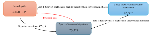
Figure 1: Proposed idea of signature inversion.

In light of Equation (2) and Theorem 2.2, a polynomial function on the truncated log-signature is equivalently expressed as a linear functional on the signature. We will provide our inversion formulae using this second representation. Throughout this section, $x:[0,1]\to\mathbb{R}$ will denote a $1$-dimensional smooth path. The results in the sequel can be naturally extended to multidimensional paths by applying the same procedure channel by channel.

Depending on the type of basis we chose to represent the path, we will often need to reparameterize the path from the interval $[0,1]$ to a specified time interval $[a,b]$ and augment it with time as well as with additional channels $c^{1},c^{2},...,c^{r}:[a,b]\to\mathbb{R}$, tailor-made for the specific type of inversion. We denote the augmented path by $\hat{x}(t)=(t,c^{1}(t),...,c^{r}(t),x(t))\in\mathbb{R}^{r+2}$. Note that these transformations are fully deterministic and do not affect the complexity of the generation task outlined in Section 2.3. Furthermore, we will use the shorthand notation $S(\hat{x})$ for the step-$n$ signature $S^{\leq n}(\hat{x})$ throughout the section, and assume that the truncation level $n$ is always high enough to retrieve the desired number of basis coefficients. All proofs can be found in Appendix C.

3.1 Inversion via Fourier coefficients

In this section, we derive closed-form expressions for retrieving the first $n$ Fourier coefficients of a path from its signature. First, recall that the Fourier series of a $2\pi$-periodic path $x(t)$ up to order $n\in\mathbb{N}$ is

$$x_{n}(t)=a_{0}+\sum_{n=1}^{n}(a_{n}\cos(nt)+b_{n}\sin(nt))$$

where $a_{0},a_{n},b_{n}$ are defined as

$$a_{0}=\frac{1}{2\pi}\int_{0}^{2\pi}x(t)dt,$$ (5)

$$a_{n}=\frac{1}{\pi}\int_{0}^{2\pi}x(t)\cos(nt)dt$$ (6)

$$b_{n}=\frac{1}{\pi}\int_{0}^{2\pi}x(t)\sin(nt)dt.$$ (7)

Theorem 3.1.

Let $x:[0,2\pi]\to\mathbb{R}$ be a periodic smooth path such that $x(0)=0$, and consider the augmentation $\hat{x}(t)=(t,\sin(t),\cos(t)-1,x(t))\in\mathbb{R}^{4}$. Then the following relations hold

$$\begin{split}a_{0}&=\frac{1}{2\pi}\langle e_{4}\succ e_{1},S(\hat{x})\rangle,\\ a_{n}&=\frac{1}{\pi}\sum_{k=0}^{n}\sum_{q=0}^{k}\binom{n}{k}\binom{k}{q}\cos(\frac{1}{2}(n-k)\pi)\langle e_{4}\shuffle e_{2}^{\shuffle n-k}\shuffle e_{3}^{\shuffle q})\succ e_{1},S(\hat{x})\rangle,\\ b_{n}&=\frac{1}{\pi}\sum_{k=0}^{n}\sum_{q=0}^{k}\binom{n}{k}\binom{k}{q}\sin(\frac{1}{2}(n-k)\pi)\langle e_{4}\shuffle e_{2}^{\shuffle n-k}\shuffle e_{3}^{\shuffle q})\succ e_{1},S(\hat{x})\rangle.\end{split}$$ (8)

3.2 Inversion via orthogonal polynomials

To accommodate path generation use cases for which a non-Fourier representation is more suitable, next we derive formulae for inverting the signature using expansions of the path in orthogonal polynomial bases. Recall that any orthogonal polynomial family $(p_{n})_{n\in\mathbb{N}}$ with a weight function $\omega:[a,b]\rightarrow\mathbb{R}$ satisfies a 3-term recurrence relation

$$p_{n}(t)=(A_{n}t+B_{n})p_{n-1}(t)+C_{n}p_{n-2}(t),\qquad n\geq 2,$$ (9)

with $p_{0}(t)=1$ and $p_{1}(t)=A_{1}t+B_{1}$. Also, note that any smooth (or at least square-integrable) path $x(t)$ with $x(a)=0$ can be approximated arbitrarily well as $x(t)\approx\sum_{n=0}^{\infty}\alpha_{n}p_{n}(t)$ where $\alpha_{n}$ is the $n$-th orthogonal polynomial coefficient

$$\alpha_{n}=\frac{1}{(p_{n},p_{n})}\int_{a}^{b}x(t)p_{n}(t)\omega(t)dt,$$ (10)

and $(\cdot,\cdot)$ denotes the inner product $(f,g)=\int_{a}^{b}f(t)g(t)\omega(t)dt$. We include several examples of such polynomial families in Appendix B.

Theorem 3.2.

Let $x:[a,b]\to\mathbb{R}$ be a smooth path such that $x(a)=0$. Consider the augmentation $\hat{x}(t)=(t,\omega(t)x(t))\in\mathbb{R}^{2}$, where $\omega(t)$ corresponds to the weight function of a system of orthogonal polynomials $(p_{n})_{n\in\mathbb{N}}$ and is well defined on the closed and compact interval $[a,b]$. Then, there exists a linear combination $\ell_{n}$ of words such that the $n^{th}$ coefficient in Equation (10) satisfies $\alpha_{n}=\langle\ell_{n},S(\hat{x})\rangle$. Furthermore, the sequence $(\ell_{n})_{n\in\mathbb{N}}$ satisfies the following recurrence relation

$$\ell_{n}=A_{n}\frac{(p_{n-1},p_{n-1})}{(p_{n},p_{n})}e_{1}\succ\ell_{n-1}+(A_{n}a+B_{n})\frac{(p_{n-1},p_{n-1})}{(p_{n},p_{n})}\ell_{n-1}+C_{n}\frac{(p_{n-2},p_{n-2})}{(p_{n},p_{n})}\ell_{n-2},$$

with

$$\ell_{0}=\frac{A_{0}}{(p_{0},p_{0})}e_{21}\quad\text{ and }\quad\ell_{1}=\frac{A_{1}}{(p_{1},p_{1})}(e_{121}+e_{211})+\frac{A_{1}a+B_{1}}{(p_{1},p_{1})}e_{21}.$$

Remark.

The results in Theorem 3.2 require signatures of $\hat{x}=(t,w(t)x(t))$. However, sometimes one may only have signatures of $\tilde{x}=(t,x(t))$. In Section C.2 we propose an alternative method by approximating the weight function as a Taylor series.

4 Related work

Multivariate time series generation

Synthesizing multivariate time series has been an active area of research in the past several years, predominantly relying on generative adversarial networks (GANs) [27]. Simple recurrent neural networks acting as generators and discriminators [46, 21] later evolved into encoder-decoder architectures where the adversarial generation happens in a learned latent space [70, 49, 34]. To synthesise time series in continuous time, architectures based on neural differential equations in the latent space [56, 68] have emerged as generalisations of RNNs. These latent ODE models suffer from limited flexibility as the initial condition fully determines the trajectory, leaving no possibility to adjust after sharp changes in the temporal dynamics. More flexible alternatives have been proposed in the forms of neural controlled differential equations [37] and state space ODEs [73]. Some alternative ways to remove the dependence on spatial resolution can also be seen in the literature, such as FourierFlows [1] which uses normalizing flows on data projected onto the Fourier frequency domain, and HyperTime [25], which learns time series embeddings as implicit neural representations (INRs).

Diffusion models for time series generation

There are a number of denoising probabilistic diffusion models (DDPMs) currently at the forefront of time series synthesis, such as DiffTime [28], which reformulates the constrained time series generation problem in terms of conditional denoising diffusion [63]. Most recently, Diffusion-TS [72] has demonstrated superior performance on benchmark datasets and long time series by disentangling temporal features via a Fourier-based training objective. To learn long-range dependencies, both the aforementioned methods use transformer [65]-based diffusion functions. Many recent efforts attempt to generalize score-based diffusion to infinite-dimensional function spaces [35, 20, 50, 40]. However, unlike their discrete-time counterparts, they have not yet been benchmarked on a variety of real-world temporal data. One exception to this is a diffusion framework proposed by Biloš et al. [5], which synthesises continuous time series by replacing the time-independent noise corruption with samples from a Gaussian process, forcing the diffusion to remain in the space of continuous functions.

Signature inversion

The uniqueness property of signatures mentioned in Section 2.4 has motivated several previous attempts to answer the question of inverting the signature transform, mostly as theoretical contributions focusing on one specific class of paths [42, 11, 43]. The only fast and scalable signature inversion strategy to date is the Insertion method [10], which provides an algorithm and theoretical error bounds for inverting piecewise linear paths. It was recently optimised [22] and released as a part of the Signatory [36] package. There are also examples of inversion via deep learning [36] and evolutionary algorithms [6], but they provide no convergence guarantees and become largely inefficient when deployed on real-world time series.

5 Experiments

In Section 5.1, we show that the newly proposed signature inversion method provides more accurate reconstructions than the previous Insertion algorithm [10, 22]. We also discuss the inversion quality and time complexity across different orthogonal polynomial classes. In Section 5.2, we run experiments to demonstrate that SigDiffusion combined with our inversion formulae generates high-quality, realistic samples, outperforming other recent diffusion models for long time series.

5.1 Inversion evaluation

We perform experiments to evaluate the proposed analytical signature inversion formulae derived in Section 3 via several families of orthogonal bases. Using example paths given by sums of random sine waves with injected Gaussian noise, we reconstruct the original paths from their step-$12$ signatures. Figure 2 compares inversion of these paths via Legendre and Fourier coefficients to the Insertion method [10, 22], showcasing the improvement in inversion quality provided by our explicit inversion formulae.

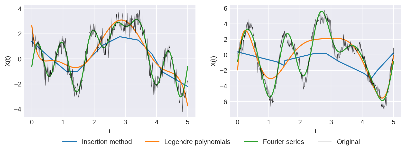
Figure 2: Comparison of different inversion methods.

Figure 3 presents the time consumption against the $L_{2}$ reconstruction error with an increasing degree of polynomials. From the plot, we see that for a given running time, signature inversion using lower-order Hermite polynomials yields superior path reconstruction compared to inversion via higher-order Jacobi polynomials. Furthermore, when comparing inversions in equal precision, the use of Hermite polynomials accelerates the process by approximately a factor of ten compared to Jacobi polynomials.

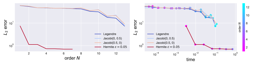
Figure 3: $L_{2}$ error of signature inversion via orthogonal polynomials with respect to the polynomial order $N$ and time. Error and time are calculated by an average of 15 paths with $200$ sample points.

Notably, the factor holding the most influence over the reconstruction quality is the truncation level of the signature, as it bounds the order of polynomials we can retrieve. Another important factor is the complexity of the underlying path. We refer the interested reader to a discussion about signature inversion quality in Appendix D. Namely, Figures 9 and 10 show more examples of inverted signatures using different types of paths and polynomial bases.

5.2 Generating long time series

In this Section, we generate step-$4$ log-signatures of 1000-point-long time series using the proposed SigDiffusion architecture. We then use inversion via Fourier coefficients proposed in Section 3.1 to invert the generated samples back to paths and compare them against other diffusion-based models. We perform experiments on 3 different time series datasets: Long sines - a benchmark dataset of 5-dimensional sine curves with randomly sampled frequency and phase [70], Predator-prey - a two-dimensional continuous system evolving according to a set of ODEs, and Household Electric Power Consumption (HEPC) [54] - a real-world dataset of household power consumption collected over 4 years at a 1-minute sampling rate. From HEPC, we pick the voltage feature to generate as a univariate time series. We use the metrics established in Yoon et al. [70]. The Discriminative score reports the out-of-sample accuracy of an RNN classifier trained to distinguish between real and generated data. The Predictive score measures the loss of a next point predictor RNN trained on the synthetic data and evaluated on the real data. We also run the Kolmogorov-Smirnov (KS) test on marginal distributions of random batches of ground truth and generated paths. We repeat this test 1000 times with a batch size of 64 and report the mean KS score with the mean Type I error for a 5% significance threshold. Since the cross-channel terms of the log-signature are not necessary for the inversion methods, we generate a concatenated vector of the log-signatures of each separate dimension plus their augmentation described in Section 3. Additional details about the experimental setup can be found in Appendix E.

Tables 1 and 2 list the time series generation performance metrics compared with three recent diffusion model architectures specifically designed to handle long or continuous-time paths: Diffusion-TS [72] and two versions of CSPD-GP [5]. CSPD-GP (RNN) and CSPD-GP (Transformer) refer to score-based diffusion models with the score function either being an RNN or a transformer. Due to memory constraints of the attention layers in transformer-based architectures, we had to halve the batch size when training Diffusion-TS and CSPD-GP (Transformer). We kept all other hyperparameters as proposed in the original works for similar datasets. The performance metrics are computed using 1000 sampled paths from each model. Table 4 shows the model sizes and training times, demonstrating that SigDiffusion outperforms the other models while also having the most efficient architecture.

Table 1: Results for generating time series of length 1000.

Dataset	Model	Discriminative Score	Predictive Score
Long sines	SigDiffusion (ours)	0.095±.023	0.096±.004
	Diffusion-TS	0.416±.046	0.147±.006
	CSPD-GP (RNN)	0.469±.005	0.111±.005
	CSPD-GP (Transformer)	0.500±.002	0.239±.015
Predator-prey	SigDiffusion (ours)	0.135±.073	0.048±.000
	Diffusion-TS	0.500±.000	0.459±.044
	CSPD-GP (RNN)	0.181±.068	0.051±.000
	CSPD-GP (Transformer)	0.498±.002	0.922±.002
HEPC	SigDiffusion (ours)	0.097±.122	0.080±.000
	Diffusion-TS	0.452±.037	0.187±.000
	CSPD-GP (RNN)	0.416±.117	0.211±.005
	CSPD-GP (Transformer)	0.500±.001	0.569±..000

Table 2: KS Test average scores and type I errors on the marginals of time series of length 1000.

Dataset	Model	t=300	t=500	t=700	t=900
Long sines	SigDiffusion (ours)	0.22, 34%	0.24, 45%	0.23, 34%	0.23, 39%
	Diffusion-TS	0.63, 98%	0.59, 98%	0.67, 99%	0.54, 98%
	CSPD-GP (RNN)	0.78, 100%	0.55, 100%	0.47, 90%	0.39, 85%
	CSPD-GP (Transformer)	0.59, 100%	0.61, 100%	0.57, 100%	0.63, 100%
Predator-prey	SigDiffusion (ours)	0.19, 13%	0.26, 55%	0.21, 30%	0.22, 33%
	Diffusion-TS	1.00, 100%	1.00, 100%	1.00, 100%	1.00, 100%
	CSPD-GP (RNN)	0.28, 62%	0.25, 46%	0.37, 91%	0.38, 89%
	CSPD-GP (Transformer)	0.80, 100%	0.78, 100%	0.79, 100%	0.74, 100%
HEPC	SigDiffusion (ours)	0.20, 16%	0.19, 11%	0.21, 21%	0.20, 19%
	Diffusion-TS	0.85, 100%	0.87, 100%	0.83, 100%	0.87, 100%
	CSPD-GP (RNN)	0.53, 100%	0.54, 100%	0.55, 100%	0.56, 100%
	CSPD-GP (Transformer)	1.00, 100%	1.00, 100%	1.00, 100%	1.00, 100%

6 Conclusion and Limitations

In this paper, we introduced SigDiffusion, a new diffusion model that gradually perturbs and denoises log-signature embeddings of long time series, preserving their Lie algebraic structure. To recover the path from its log-signature, we proved that the coefficients in the expansion of a path in a given basis, such as Fourier or orthogonal polynomials, can be expressed as explicit linear functionals on the signature, or equivalently as polynomial functions on the log-signature. These results provide explicit signature inversion formulae, representing a major improvement over signature inversion algorithms previously proposed in the literature. Finally, we demonstrated how combining SigDiffusion with these inversion formulae provides a powerful generative approach for time series that is competitive with state-of-the-art diffusion models for temporal data.

As this is the first work on diffusion models for time series using signature embeddings, there are still many research directions to explore. For instance, it would be interesting to consider other types of path-developments embedding temporal signals to (compact) Lie groups, such as the ones considered in the recent paper [9]. By avoiding the exponential explosion in the number of features, these recent alternatives might provide representations of signals than are more parsimonious than the signature, although it is unclear how an inversion mechanism would work in these cases. Another compelling research direction would be to consider diffusion models specifically designed for data living on Lie groups, such as the ones proposed by [33]. Finally, it would be interesting to understand how discrete-time signatures [19] could be leveraged to encode discrete sequences on Lie groups and leverage this encoding to perform diffusion-based generative modelling for text.

Appendix

This appendix is structured in the following way. In Section A we complement the material presented in Section 2 by adding additional details on the signature. In Section B, we provide examples of orthogonal polynomial families one can use for signature inversion due to the derived inversion formulae in Section 3. In Section C we provide proofs for the signature inversion Theorem 3.1 and Theorem 3.2. Section D contains additional examples and discussion about the quality of signature inversion by different bases. Section E provides details on the implementation of experiments.

Appendix A Additional details on the signature

We begin by providing simple examples of signature computations.

A.1 Simple examples of signature computations

In the following examples, we alter the notation so that for a path $x:[a,t]\rightarrow\mathbb{R}^{d}$, the tensor representing the $k$-th level of the signature computed on an interval $[a,t]$ is denoted as

$$S(x)^{(k)}_{a,t}=(S(x)^{i_{1},\dots,i_{k}}_{a,t}:i_{1},\dots,i_{k}\in\{1,\dots,d\})\in(\mathbb{R}^{d})^{\otimes k}.$$ (11)

Furthermore, we can express the value of $S(x)^{(k)}_{a,t}$ at a particular set of indices $i_{1},\dots,i_{k}\in\{1,\dots d\}$ as a k-fold iterated integral

$$S(x)^{i_{1},\dots,i_{k}}_{a,t}=\int_{a<t_{1}<\dots<t_{k}<t}dx^{i_{1}}_{t_{1}}\dots dx^{i_{k}}_{t_{k}}.$$

We assume that the signature is always truncated at a sufficiently high level $n$, allowing us to denote the step-$n$ signature simply as

$$S(x)_{a,t}=(1,S(x)^{(1)}_{a,t},S(x)^{(2)}_{a,t},S(x)^{(3)}_{a,t},\dots,S(x)^{(n)}_{a,t})\in T_{1}^{n}(\mathbb{R}^{d}).$$ (12)

Example A.1 (Geometric interpretation of a 2-dimensional path).

Consider a path $\hat{x}:[0,9]\rightarrow\mathbb{R}^{2}$, where $\hat{x}=(x_{t}^{1},x_{t}^{2})=(t,x(t))$. Here, $x(t)$ is defined as

$$x_{t}^{2}=x(t)=\begin{cases}\sqrt{3}t\qquad&t\in[0,2]\\ 2\sqrt{3}\qquad&t\in[2,8]\\ \sqrt{3}t-6\sqrt{3}\qquad&t\in[8,9]\end{cases},$$

which is continuous and piecewise differentiable. In this case, $\dot{x}_{t}^{1}=1$, and $\dot{x}_{t}^{2}$ can be expressed as

$$\dot{x}_{t}^{2}=\dot{x}(t)=\begin{cases}\sqrt{3}\qquad&t\in(0,2)\\ 0\qquad&t\in(2,8)\\ \sqrt{3}\qquad&t\in(8,9)\end{cases}.$$

One can compute the step-$n$ signature of $\hat{x}$ as

$$S(\hat{x})_{0,9} =(1,S(\hat{x})^{(1)}_{0,9},S(\hat{x})^{(2)}_{0,9},S(\hat{x})^{(3)}_{0,9},\dots,S(\hat{x})^{(n)}_{0,9})$$

$$=(1,S(\hat{x})^{1}_{0,9},S(\hat{x})^{2}_{0,9},S(\hat{x})^{1,2}_{0,9},S(\hat{x})^{2,1}_{0,9},S(\hat{x})^{1,1,1}_{0,9},\dots,S(\hat{x})_{0,9}^{i_{1},\ldots,i_{n}}),$$

where

$$S(\hat{x})^{1}_{0,9}=\int_{0<s<9}dx^{1}_{s}=x^{1}_{9}-x^{1}_{0}=9$$

$$S(\hat{x})^{2}_{0,9}=\int_{0<s<9}dx^{2}_{s}=x^{2}_{9}-x^{2}_{0}=3\sqrt{3}$$

$$S(\hat{x})^{1,1}_{0,9}=\int_{0<r<s<9}dx^{1}_{r}dx^{1}_{s}=\int_{0<s<9}x^{1}_{s}dx^{1}_{s}=\frac{1}{2}\left(x^{1}_{s}\right)^{2}\biggr{|}_{0}^{9}=\frac{81}{2}$$

$$S(\hat{x})^{1,2}_{0,9}=\int_{0<r<s<9}dx^{1}_{r}dx^{2}_{s}=\int_{0<s<9}sdx^{2}_{s}=\int_{0<s<9}s\dot{x}^{2}_{s}ds=\frac{\sqrt{3}}{2}s^{2}\biggr{|}_{0}^{2}+\frac{\sqrt{3}}{2}s^{2}\biggr{|}_{8}^{9}=\frac{21}{2}\sqrt{3}$$

$$S(\hat{x})^{2,1}_{0,9}=\int_{0<r<s<9}dx^{2}_{r}dx^{1}_{s}=\int_{0<s<9}x^{2}_{s}ds=\frac{\sqrt{3}}{2}s^{2}\biggr{|}_{0}^{2}+2\sqrt{3}s\biggr{|}_{2}^{8}+\frac{\sqrt{3}}{2}s^{2}-6\sqrt{3}s\biggr{|}_{8}^{9}=\frac{33}{2}\sqrt{3}$$

$$S(\hat{x})^{2,2}_{0,9}=\int_{0<r<s<9}dx^{2}_{r}dx^{2}_{s}=\int_{0<s<9}x^{2}_{s}dx^{2}_{s}=\frac{1}{2}\left(x^{2}_{s}\right)^{2}\biggr{|}_{0}^{9}=\frac{27}{2}.$$

From Figure 4, let $A_{-}$ and $A_{+}$ represent the signed value of the shaded region. The signed Lévy area of the path is defined as $A_{-}+A_{+}$. In this case, the signed Lévy area is $-3\sqrt{3}$. Surprisingly,

$$\frac{1}{2}\left(S(\hat{x})^{1,2}_{0,9}-S(\hat{x})^{2,1}_{0,9}\right)=\frac{1}{2}\left(\frac{21}{2}\sqrt{3}-\frac{33}{2}\sqrt{3}\right)=-3\sqrt{3}=A_{-}+A_{+},$$

which is exactly the signed Lévy area.

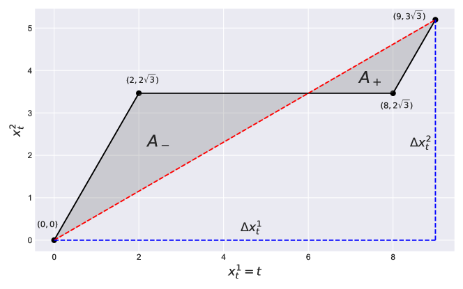
Figure 4: Path in Example A.1. The shaded region represents the signed Lévy area.

Another important example is given by the signature of linear paths.

Example A.2 (Signatures of linear paths).

Suppose there is a linear path $x:[a,b]\to\mathbb{R}^{d}$. Then the path $x$ is linear in terms of $t$, i.e.

$$x_{t}=x_{a}+\frac{t-a}{b-a}\left(x_{b}-x_{a}\right).$$

It follows that its derivative can be written as

$$dx_{t}=\frac{\left(x_{b}-x_{a}\right)}{b-a}dt.$$

Recalling the definition of a signature, it holds that

$$S(x)^{i_{1},\dots,i_{k}}_{a,b} =\int_{a<t_{1}<\dots<t_{k}<b}dx^{i_{1}}_{t_{1}}\dots dx^{i_{k}}_{t_{k}}$$

$$=\frac{\prod_{j=1}^{k}\left(x_{b}^{i_{j}}-x_{a}^{i_{j}}\right)}{(b-a)^{k}}\int_{a<t_{1}<\dots<t_{k}<b}dt_{1}\dots dt_{k}$$

$$=\frac{\prod_{j=1}^{k}\left(x_{b}^{i_{j}}-x_{a}^{i_{j}}\right)}{(b-a)^{k}}\frac{(b-a)^{k}}{k!}$$

$$=\frac{\prod_{j=1}^{k}\left(x_{b}^{i_{j}}-x_{a}^{i_{j}}\right)}{k!}.$$

Therefore, the whole step-$n$ signature can be expressed as a tensor exponential of the linear increment $x_{b}-x_{a}$

$$S(x)^{(k)}_{a,b} =\frac{\left(x_{b}-x_{a}\right)^{\otimes k}}{k!},$$

$$S(x)_{a,b} =\sum_{k=0}^{n}\frac{\left(x_{b}-x_{a}\right)^{\otimes k}}{k!}$$

$$=\exp_{\otimes}\left(x_{b}-x_{a}\right).$$

Chen’s identity in Theorem 2.3 is one of the most fundamental algebraic properties of the signature as it describes the behaviour of the signature under the concatenation of paths.

Definition A.1 (Concatenation).

Consider two smooth paths $x:[a,b]\to\mathbb{R}^{d}$ and $y:[b,c]\to\mathbb{R}^{d}$. Define the concatenation of $x$ and $y$, denoted by $x\ast y$ as a path $[a,c]\rightarrow\mathbb{R}^{d}$

$$(x\ast y)_{t}:=\begin{cases}x_{t}\qquad&\text{ if }a\leq t\leq b\\ x_{b}-{y}_{b}+y_{t}\qquad&\text{ if }b\leq t\leq c\end{cases}.$$

Chen’s identity in Theorem 2.3 provides a method to simplify the analysis of longer paths by converting them into manageable shorter ones. If we have a smooth path $x:[t_{0},t_{n}]\rightarrow\mathbb{R}^{d}$, then inductively, we can decompose the signature of $x$ to

$$S(x)_{t_{0},t_{n}}=S(x)_{t_{0},t_{1}}\cdot S(x)_{t_{1},t_{2}}\cdot\cdots\cdot S(x)_{t_{n-1},t_{n}}.$$

Moreover, if we have a time series $(t_{0},x_{0}),...,(t_{n},x_{n})\in\mathbb{R}^{d+1}$, we can treat $x$ as a piecewise linear path interpolating the data. Based on Example A.2, one can observe that

$$S(x)_{t_{0},t_{n}}=\exp_{\otimes}\left(x_{t_{1}}-x_{t_{0}}\right)\cdot\exp_{\otimes}\left(x_{t_{2}}-x_{t_{1}}\right)\cdot\cdots\cdot\exp_{\otimes}\left(x_{t_{n}}-x_{t_{n-1}}\right),$$

which is widely used in Python packages such as esig or iisignature.

Example A.3 (Example of shuffle identity).

Consider a smooth path $x=(x^{1}_{t},x^{2}_{t}):[a,b]\to\mathbb{R}^{2}$ .

$$\langle e_{1},S(x)_{a,b}\rangle\langle e_{2},S(x)_{a,b}\rangle =\int_{a<t<b}dx^{1}_{t}\int_{a<t<b}dx^{2}_{t}$$

$$=\int_{a<t<b}\dot{x}^{1}_{t}dt\int_{a<t<b}\dot{x}^{2}_{t}dt$$

$$\overset{\mathrm{by\,parts}}{=}\int_{a<t<b}\langle e_{2},S(x)_{a,t}\rangle\dot{x}^{1}_{t}dt+\int_{a<t<b}\langle e_{1},S(x)_{a,t}\rangle\dot{x}^{2}_{t}dt$$

$$=\langle e_{2,1},S(x)_{a,b}\rangle+\langle e_{1,2},S(x)_{a,b}\rangle.$$

By the shuffle identity, we have

$$\langle e_{1},S(x)_{a,b}\rangle\langle e_{2},S(x)_{a,b}\rangle =\langle e_{1},S({x})_{a,b}\rangle\langle e_{2},S({x})_{a,b}\rangle$$

$$=\langle e_{1}\shuffle e_{2},S({x})_{a,b}\rangle$$

$$=\langle e_{1,2}+e_{2,1},S({x})_{a,b}\rangle$$

$$=\langle e_{1,2},S(x)_{a,b}\rangle+\langle e_{2,1},S(x)_{a,b}\rangle,$$

which is exactly the same as what we derived via integration by parts.

Example A.4 (Example of half-shuffle computations).

Consider a two-dimensional real-valued smooth path $\hat{x}=(t,x(t)):[a,b]\rightarrow\mathbb{R}^{2}$ with $x(a)=0$. The first-level signature can computed as follows:

$$\langle e_{1},S(\hat{x})_{a,t}\rangle=\int_{a}^{t}ds=t-a,\quad\langle e_{2},S(\hat{x})_{a,t}\rangle=\int_{a}^{t}d\left(x(s)\right)=x(t)-x(a)=x(t).$$

Then, one can express all integrals in terms of powers of $t-a$ and $x(t)$ by signatures of $\hat{x}$. For example, let $n,m\in\mathbb{N}_{0}$,

$$\int^{b}_{a}(t-a)^{n}x(t)^{m}dt =\int^{b}_{a}(t-a)^{n}x(t)^{m}d(t-a)$$

$$=\int^{b}_{a}\left(\langle e_{1},S(\hat{x})_{a,t}\rangle\right)^{n}\left(\langle e_{2},S(\hat{x})_{a,t}\rangle\right)^{m}d\left(\langle e_{1},S(\hat{x})_{a,t}\rangle\right)$$

$$=\langle\left(e_{1}^{\shuffle n}\shuffle e_{2}^{\shuffle m}\right)\succ e_{1},S(\hat{x})_{a,b}\rangle,$$

which is followed by the shuffle identity and right half-shuffle product in integrals.

Appendix B Orthogonal polynomials and Fourier series

In this section, we introduce the background material on orthogonal polynomials and the Fourier series necessary for the signature inversion formulae presented in the next section.

B.1 Orthogonal polynomials

B.1.1 Inner product and orthogonality

Consider a dot product $(x,y)=\sum_{i=1}^{n}x_{i}y_{i}$, where ${x},{y}\in\mathbb{R}^{n}$. If weights $w_{1},\cdots,w_{n}\in\mathbb{R}_{+}$ are defined, $(x,y)_{w}=\sum_{i=1}^{n}w_{i}x_{i}y_{i}$ is measured as a weighted dot product, where $(\cdot,\cdot)_{w}$ can be written as $(\cdot,\cdot)$ for simplicity.

For $p\in[1,\infty)$, $L^{p}_{w}(\Omega)$ is the linear space of measurable functions from $\Omega$ to $\mathbb{R}$ such that their weighted $p$-norms are bounded, i.e.

$$L^{2}_{w}(\Omega)=\left\{v\text{ is measurable in }\Omega\biggr{|}\int_{\Omega}|v(t)|^{2}w(t)dt<\infty\right\}.$$

For example, let $d\alpha$ be a non-negative Borel measure supported on the interval $[a,b]$ and $\mathbb{V}=L^{2}_{w}(a,b)$. One can define $(f,g)=\int_{a}^{b}f(t)g(t)d\alpha(t)$ as a Stieltjes integral for all $f,g\in\mathbb{V}$. Note that if $\alpha(t)$ is absolutely continuous, which will be the setting throughout this section, then one can find a weight density $w(t)$ such that $d\alpha(t)=w(t)dt$. In this case, the definition of inner product over a function space reduces to an integral with respect to a weight function, i.e.

$$(f,g)=\int_{a}^{b}f(t)g(t)w(t)dt.$$

We can then refer an orthogonal polynomial system to be orthogonal with respect to the weight function $w$. We denote $\mathbb{P}[t]\subset L^{2}_{w}(\Omega)$ as the space of all polynomials. A polynomial of degree $n$, $p\in\mathbb{P}_{n}[t]$, is monic if the coefficient of the $n$-th degree is one.

Definition B.1 (Orthogonal polynomials).

For an arbitrary vector space $\mathbb{V}$, $u$ and $v$ are orthogonal if $(u,v)=0$ with all $u,v\in\mathbb{V}$. When $\mathbb{V}=\mathbb{P}[t]$, a sequence of polynomials $(p_{n})_{n\in\mathbb{N}}\in\mathbb{P}[t]$ is called orthogonal polynomials with respect to a weight $w$ if for all $m\neq n$,

$$(p_{n},p_{m})=\int p_{n}(t)p_{m}(t)w(t)dt=0,$$

where $\text{deg}(p_{n})=n$ is the degree of a polynomial. Furthermore, we say the sequence of orthogonal polynomials is orthonormal if $(p_{n},p_{n})=1$ for all $n\in\mathbb{N}$.

For simplification, the inner product notation $(\cdot,\cdot)$ will be used without specifying the integral formulation for the orthogonal polynomials. To construct a sequence of orthogonal polynomials in Definition B.1, one can follow the Gram-Schmidt orthogonalisation process, which is stated below.

Theorem B.1 (Gram-Schmidt orthogonalisation).

The polynomial system $(p_{n})_{n\in\mathbb{N}}$ with respect to the inner product $(\cdot,\cdot)$ can be constructed recursively by

$$p_{0}=1,\qquad p_{n}=t^{n}-\sum_{i=1}^{n-1}\frac{(t^{n},p_{i})}{(p_{i},p_{i})}p_{i}\quad\text{for }n\geq 1$$ (13)

From the orthogonalisation process in Theorem B.1, we can see that the $n$-th polynomial $p_{n}$ has degree $n$ exactly, which means $(p_{n})_{n\in\mathbb{N}}$ is a basis spanning $\mathbb{P}[t]$. Furthermore, the orthogonal construction makes the orthogonal polynomial system an orthogonal basis with respect to the corresponding inner product. The following proposition forms an explicit expression for coefficients of $(p_{k})_{k\in\{0,\cdots,n\}}$ in an arbitrary $n$-th degree polynomial.

Proposition B.1.1 (Orthogonal polynomial expansion).

Consider an arbitrary polynomial $x(t)\in\mathbb{P}_{n}[t]$. One can express $x(t)$ by a sequence of orthogonal polynomials $(p_{k})_{k\in\{0,\cdots,n\}}$, i.e.

$$x(t)=\sum_{k=0}^{n}\frac{(p_{k},x)}{(p_{k},p_{k})}p_{k}(t).$$

Remark.

We have stated the orthogonal polynomial expansion for $x\in\mathbb{P}_{n}[t]$. In general, by the closure of orthogonal polynomial systems in $L^{2}_{w}(a,b)$, arbitrary $f\in L^{2}_{w}(a,b)$ can be written as an infinite sequence of orthogonal polynomials.

$$f(t)=\sum_{k=0}^{\infty}\frac{(p_{k},f)}{(p_{k},p_{k})}p_{k}(t).$$

The $N$-th degree approximation of $f$ is the best approximating polynomial with a degree less or equal to $N$, denoted by

$$P_{N}f(t)=\sum_{k=0}^{N}\frac{(p_{k},f)}{(p_{k},p_{k})}p_{k}(t).$$ (14)

B.1.2 Basic properties

Here, we will list the main properties of orthogonal polynomials significant for our application.

The three-term recurrence relation

Theorem B.2 (Three-term recurrence relation).

A system of orthogonal polynomials $(p_{n})_{n\in\mathbb{N}}$ with respect to a weight function $w$ satisfies the three-term recurrence relation.

$$p_{0}(t)=1,\quad p_{1}(t)=A_{1}t+B_{1},\quad p_{n+1}(t)=(A_{n+1}t+B_{n+1})p_{n}(t)+C_{n+1}p_{n-1}(t),$$

for all $n\in\mathbb{N}$, and $A_{i}>0$ for all $i\in\mathbb{N}_{0}$.

Before proving the recurrence relation, we will first show that an orthogonal polynomial is orthogonal to all polynomials with a degree lower than that of itself.

Lemma B.2.1.

A polynomial $q(t)\in\mathbb{P}_{n}[t]$ satisfies $(q,r)=0$ for all $r(t)\in\mathbb{P}_{m}[t]$ with $m<n$ if and only if $q(t)=p_{n}(t)$ up to some constant coefficient, where $p_{n}(t)$ denotes the orthogonal polynomial with degree $n$.

Proof.

$\Longrightarrow$: Consider $q(t)=\alpha_{n}t^{n}+O(t^{n-1})$ and $p_{n}(t)=\tilde{\alpha}_{n}t^{n}+O(t^{n-1})$. Then we define

$$s(t)=q(t)-\frac{\alpha_{n}}{\tilde{\alpha}_{n}}p_{n}(t)=O(t^{n-1}),$$

which has a degree at most $n-1$. Therefore, for all $m<n$,

$$(s,p_{m})=(q,p_{m})-\frac{\alpha_{n}}{\tilde{\alpha}_{n}}(p_{n},p_{m})=0.$$

The former inner product $(q,p_{m})=0$ by assumption, while the latter inner product $(p_{n},p_{m})=0$ by orthogonality. By Proposition B.1.1,

$$s(t)=\sum_{m=0}^{n-1}\frac{(p_{m},s)}{(p_{m},p_{m})}p_{m}(t)=0\quad\implies\quad q(t)=\frac{\tilde{\alpha}_{n}}{\alpha_{n}}p_{n}(t).$$

$\Longleftarrow$: Consider $r(t)=\sum_{k=0}^{m}r_{k}p_{k}(t)$. Let $q(t)=cp_{n}(t)$. Using the linearity of the inner product and orthogonality of $(p_{n})_{n\in\mathbb{N}}$, for all $m<n$,

$$(q,r)=\left(cp_{n}(t),\sum_{k=0}^{m}r_{k}p_{k}(t)\right)=c\sum_{k=0}^{m}r_{k}(p_{n}(t),p_{k}(t))=0.$$

∎

Now, we have enough tools to prove the famous three-term recurrence relation.

Proof of Theorem B.2.

Consider a sequence of orthogonal polynomials $(p_{n})_{n\in\mathbb{N}}$. When $n=1$, $p_{1}$ can be expressed as $A_{1}t+B_{1}$ for $A_{1},B_{1}\in\mathbb{R}$. This is because $p_{1}$ is an element in an orthogonal basis with degree $1$. Based on the inner product of orthogonal polynomials,

$$(p_{k},tp_{n})=\int tp_{k}(t)p_{n}(t)w(t)dt=(tp_{k},p_{n}).$$

Therefore, for $0\leq k<n-1$, we have $(p_{k},tp_{n})=0$ by Lemma B.2.1. Since $tp_{n}(t)$ has degree $n+1$, by Proposition B.1.1,

$$tp_{n}(t)=\sum_{k=0}^{n+1}\frac{(p_{k},tp_{n})}{(p_{k},p_{k})}p_{k}(t)=\sum_{k=n-1}^{n+1}\frac{(p_{k},tp_{n})}{(p_{k},p_{k})}p_{k}(t)=\alpha_{n-1}p_{n-1}(t)+\alpha_{n}p_{n}(t)+\alpha_{n+1}p_{n+1}(t)$$

$$\implies p_{n+1}=\left(\frac{1}{\alpha_{n+1}}t-\frac{\alpha_{n}}{\alpha_{n+1}}\right)p_{n}(t)-\frac{\alpha_{n-1}}{\alpha_{n+1}}p_{n-1}(t),$$

which completes the proof. ∎

Remark.

Recurrence is the core property of orthogonal polynomials in our setting, as one can find higher-order coefficients based on lower-order coefficients given the analytical form of the orthogonal polynomials. This idea coincides with the shuffle identity of signatures. As stated in Theorem 3.2, one can construct an explicit recurrence relation for coefficients of orthogonal polynomials by linear functionals acting on signatures.

Approximation results for functions in $L_{w}^{2}$

Without loss of generality, consider $f\in L^{2}_{w}(-1,1)$, as we can always transform an arbitrary interval $[a,b]$ linearly into the interval $[-1,1]$. Recall the $N$-th degree approximation $P_{N}f(t)$ defined in Equation (14). The uniform convergence of the $N$-th degree approximation $P_{N}f(t)$ to $f$ can be found in [4], where we obtain

$$\frac{1}{\sqrt{2\pi}}\|f-P_{N}f\|_{2}\leq\|f-P_{N}f\|_{\infty}\leq(1+\|P_{N}\|)\|f-q\|_{\infty},\qquad q\in\mathbb{P}_{N},$$

where $\|P_{N}\|$ relates to the system of orthogonal polynomials, and $\|f-q\|_{\infty}$ depends on the smoothness of $f$. In the case of Chebyshev polynomials, where the weight function is $w(t)=1/\sqrt{1-t^{2}}$, $\|P_{N}\|=\frac{4}{\pi}\log n+\mathcal{O}(1)$ [4]. For some $\alpha\in(0,1]$,

$$\|f-P_{N}f\|_{2}\leq c_{k}\frac{\log N}{N^{k+\alpha}}\qquad\text{ for }N\geq 2.$$

The bound result is shown numerically in Figure 5.

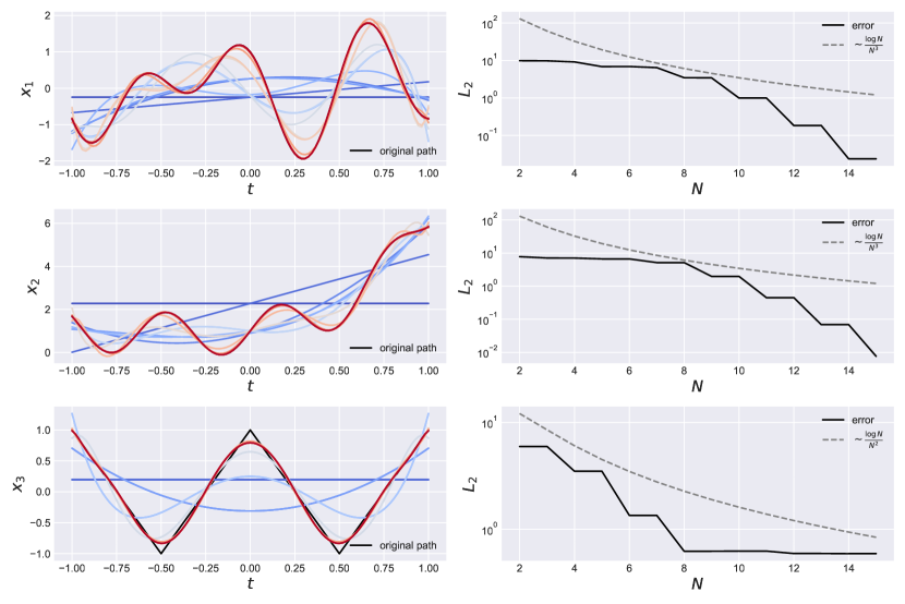
Figure 5: Approximation (left) and convergence of $L_{2}$ error (right) results for Chebyshev polynomials with increasing degree $N$. As $N$ increases, the colours change from blue to red in the left plots. Paths are given by (from top to bottom): $x_{1}(t)=\cos(10t)-\sin(2\pi t)$, $x_{2}(t)=\sin(10t)+e^{2t}-t$, $x_{3}(t)=2|2t-1|-1$.

B.1.3 Examples

In this subsection, we will provide two general orthogonal polynomial families, Jacobi polynomials and Hermite polynomials, which will be used for signature inversion in the next section. Figure 6 visualises the first few polynomials of these two kinds.

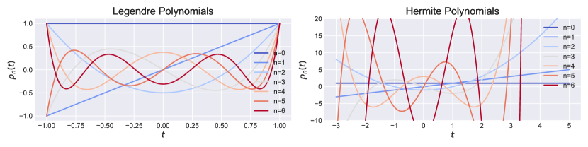
Figure 6: Visualisation of the first $7$ Legendre and Hermite polynomials.

Jacobi polynomials

Jacobi polynomials $p_{n}^{(\alpha,\beta)}$ are a system of orthogonal polynomials with respect to the weight function $w:(-1,1)\rightarrow\mathbb{R}$ such that

$$w(t;\alpha,\beta)=(1-t)^{\alpha}(1+t)^{\beta}.$$

There are many well-known special cases of Jacobi polynomials, such as Legendre polynomials $p_{n}^{(0,0)}$ and Chebyshev polynomials $p_{n}^{(-1/2,-1/2)}$. In general, the analytical expression of Jacobi polynomials [31] is defined by the hypergeometric function ${}_{2}F_{1}$:

$$p_{n}^{(\alpha,\beta)}(t)=\frac{(\alpha+1)_{n}}{n!}{}_{2}F_{1}(-n,1+\alpha+\beta+n;\alpha+1;\frac{1}{2}(1-t)),$$

where $(\alpha+1)_{n}$ is the Pochhammer’s symbol. For orthogonality, Jacobi polynomials satisfy

$$\int_{-1}^{1}(1-t)^{\alpha}(1+t)^{\beta}p_{m}^{(\alpha,\beta)}(t)p_{n}^{(\alpha,\beta)}(t)=\frac{2^{\alpha+\beta+1}\Gamma(n+\alpha+1)\Gamma(n+\beta+1)}{(2n+\alpha+\beta+1)\Gamma(n+\alpha+\beta+1)n!}\delta_{nm},\qquad\alpha,\beta>-1,$$

where $\delta_{mn}$ is the Kronecker delta. For fixed $\alpha,\beta$, the recurrence relation of Jacobi polynomials is

$$p_{n}^{(\alpha,\beta)}(t)= \frac{2n+\alpha+\beta-1}{2n(n+\alpha+\beta)(2n+\alpha+\beta-2)}\left((2n+\alpha+\beta)(2n+\alpha+\beta-2)t+\alpha^{2}-\beta^{2}\right)p_{n-1}^{(\alpha,\beta)}(t)$$

$$-\frac{(n+\alpha-1)(n+\beta-1)(2n+\alpha+\beta)}{n(n+\alpha+\beta)(2n+\alpha+\beta-2)}p_{n-2}^{(\alpha,\beta)}(t).$$

Hermite polynomials

Hermite polynomials are a system of orthogonal polynomials with respect to the weight function $w:(-\infty,\infty)\rightarrow\mathbb{R}$ such that $w(t)=\exp(-{t^{2}}/{2})$. These are called the probabilist’s Hermite polynomials, which we will use throughout the section. There is another form called the physicist’s Hermite polynomials with respect to the weight function $w(t)=\exp(-t^{2})$. The explicit expression of the probabilist’s Hermite polynomials can be written as

$$H_{n}(t)=n!\sum_{m=0}^{\lfloor\frac{n}{2}\rfloor}\left(-\frac{1}{2}\right)^{m}\frac{t^{n-2m}}{m!(n-2m)!},$$

with the orthogonality property

$$\int_{-\infty}^{\infty}H_{m}(t)H_{n}(t)e^{-\frac{t^{2}}{2}}dt=\sqrt{2\pi}n!\delta_{mn}.$$ (15)

Lastly, we state the recurrence relation of Hermite polynomials as $H_{n+1}(t)=xH_{n}(t)-nH_{n-1}(t)$. Note that the weight of Hermite polynomials can be viewed as an unnormalised normal distribution. If we are more interested in a particular region far away from the origin, we can define a “shift-and-scale” version of Hermite polynomials with respect to the weight

$$w^{t_{0},\epsilon}(t)=\exp((t-t_{0})^{2}/2\epsilon^{2}),$$

where $t_{0}$ denotes the new centre and $\epsilon$ measures standard deviation. Let $(H_{n}^{t_{0},\epsilon})_{n\in\mathbb{N}}$ denote the shift-and-scale Hermite polynomials. Then, the orthogonality property is

$$\int_{-\infty}^{\infty}H^{t_{0},\epsilon}_{m}(t)H^{t_{0},\epsilon}_{n}(t)e^{-\frac{(t-t_{0})^{2}}{2\epsilon^{2}}}dt=\epsilon\int_{-\infty}^{\infty}H^{t_{0},\epsilon}_{m}(t_{0}+\epsilon y)H^{t_{0},\epsilon}_{n}(t_{0}+\epsilon y)e^{-\frac{y^{2}}{2}}dy,$$

by substitution $y=(t-t_{0})/\epsilon$. Hence, if

$$H^{t_{0},\epsilon}_{n}(t_{0}+\epsilon y)=H_{n}(y),\qquad n\in\mathbb{N},$$ (16)

then $(H_{n}^{t_{0},\epsilon})_{n\in\mathbb{N}}$ is an orthogonal polynomial system with orthogonality

$$\int_{-\infty}^{\infty}H^{t_{0},\epsilon}_{m}(t)H^{t_{0},\epsilon}_{n}(t)e^{-\frac{(t-t_{0})^{2}}{2\epsilon^{2}}}dt=\epsilon\int_{-\infty}^{\infty}H_{m}(y)H_{n}(y)e^{-\frac{y^{2}}{2}}dy=\epsilon\sqrt{2\pi}n!\delta_{mn},$$

which follows from the orthogonality of Hermite polynomials in Equation (15). Similarly, the connection between Hermite and shift-and-scale Hermite polynomials in Equation (16) provides a way to find the explicit form and recurrence relation of $(H_{n}^{t_{0},\epsilon})_{n\in\mathbb{N}}$, which are

$$H^{t_{0},\epsilon}_{n}(t)=n!\sum_{m=0}^{\lfloor\frac{n}{2}\rfloor}\left(-\frac{1}{2}\right)^{m}\frac{1}{m!(n-2m)!}\left(\frac{t-t_{0}}{\epsilon}\right)^{n-2m},$$ (17)

$$H^{t_{0},\epsilon}_{n+1}(t)=\frac{1}{\epsilon}(t-t_{0})H^{t_{0},\epsilon}_{n}(t)-nH^{t_{0},\epsilon}_{n-1}(t).$$ (18)

Remark.

Note that there is a simple expression for $(H_{n}^{t_{0},\epsilon})_{n\in\mathbb{N}}$ at $t=t_{0}$. One can easily observe that

$$H^{t_{0},\epsilon}_{n}(t_{0})=\begin{cases}\left(-\frac{1}{2}\right)^{\frac{n}{2}}\frac{n!}{\frac{n}{2}!}\qquad&\text{for even }n\\ 0\qquad&\text{for odd }n\end{cases}.$$

B.2 Fourier series

One can also represent a function by a trigonometric series. Here, we only present a brief introduction to the Fourier series, providing complementary details to the main result in Theorem 3.1.

B.2.1 Trigonometric series

Let $f\in L^{1}(-\pi,\pi)$. The Fourier series of $f$ is defined by

$$F(t)=\frac{a_{0}}{2}+\sum_{k=1}^{\infty}\left(a_{k}\cos(kt)+b_{k}\sin(kt)\right),$$

where

$$a_{k}=\frac{1}{\pi}\int_{-\pi}^{\pi}f(t)\cos(kt)dx,\qquad k\geq 0$$

$$b_{k}=\frac{1}{\pi}\int_{-\pi}^{\pi}f(t)\sin(kt)dx,\qquad k\geq 1,$$

which can be derived from the orthogonal bases $\{\cos{kt}\}_{k}$ and $\{\sin{kt}\}_{k}$. More generally, we can extend the period to $2l\in\mathbb{R}$. For $f\in L^{1}(-l,l)$ and $k\in\mathbb{Z}$,

$$F(t)=\sum_{n=-\infty}^{\infty}c_{k}e^{i\frac{2\pi}{l}kt},\qquad c_{k}=\frac{1}{l}\int_{0}^{l}f(t)e^{-i\frac{2\pi}{l}kt}dt.$$ (19)

In the setting of the Fourier series, the expression for the $k$-th coefficient $c_{k}$ in the exponential form can be defined as a linear functional $\mathcal{L}_{k}(x)=c_{k}^{x}$ on the space of Fourier series, for $x\in L^{1}(-l,l)$.

B.2.2 Convergence

Note that $F(t)$ and $f(t)$ are closely related. Under some regularity conditions, $F(t)$ converges to $f(t)$. But in other cases, $F(t)$ may not converge to $f(t)$ or even a limit [4]. To examine the convergence of the Fourier series, we define the partial sum of the Fourier series as

$$S_{N}f(t)=\frac{a_{0}}{2}+\sum_{k=1}^{N}\left(a_{k}\cos(kt)+b_{k}\sin(kt)\right).$$

Now we present pointwise convergence and uniform convergence results [4] of the Fourier series for various functions.

Theorem B.3 (Pointwise convergence for bounded variation).

For a $2\pi$-periodic function $f$ of bounded variation on $[-\pi,\pi]$, its Fourier series at an arbitrary $t$ converges to

$$\frac{1}{2}\left(f(t^{-})+f(t^{+})\right).$$

Theorem B.4 (Uniform convergence for piecewise smooth functions).

If $f$ is a $2\pi$-periodic piecewise smooth function,

1. if $f$ is also continuous, then the Fourier series converges uniformly and continuously to $f$;

2. if $f$ is not continuous, then the Fourier series converges uniformly to $f$ on every closed interval without discontinuous points.

Theorem B.5 (Uniform error bounds).

Let $f\in C_{p}^{k,\alpha}(2\pi)$ be a $2\pi$-periodic $k$ times continuously differentiable function that is Hölder continuous with the exponent $\alpha\in(0,1]$. Then, the $2$-norm and infinity-norm bound of the partial sum $S_{N}f$ can be expressed as

$$\frac{1}{\sqrt{2\pi}}\|f-S_{N}f\|_{2}\leq\|f-S_{N}f\|_{\infty}\leq c_{k}\frac{\log N}{N^{k+\alpha}},\qquad\text{ for }N\geq 2.$$

For functions only defined in an interval $[a,b]$, we can always shift and extend them to be $2\pi$-periodic functions. These theorems guarantee the convergence of common functions we will use in later experiments. To illustrate this, Figure 7 shows how the convergence theories match with numerical results. In particular, note that compared with the path $x_{2}(t)=\sin(10t)+e^{2t}-t$, the other 2 paths have better convergence results. The main reason is that the Fourier series of $x_{2}$ at $t=\pm 1$ does not pointwise converge to $x_{2}(\pm 1)$. Since the Fourier series treats the interval $[-1,1]$ as one period over $\mathbb{R}$, by Theorem B.3, the series will converge to $(x_{2}(-1)+x_{2}(1))/2$ at $t=\pm 1$, leading to incorrect convergence at boundaries. This property also arises in real-world non-periodic time series, leading us to introduce the mirror augmentation later in Appendix E.

Comparing Figures 5 and 7, one can observe that orthogonal polynomials are better at approximating continuously differentiable paths, while Fourier series coefficients are better at estimating paths with spikes, and their computation is more stable in the long run. In a later section, Figure 8 provides a summary of convergence results for different types of orthogonal polynomials and Fourier series, which also match the results shown here.

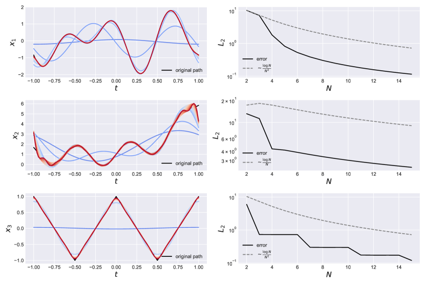
Figure 7: Approximation (left) and $L_{2}$ convergence (right) results for Fourier series by increasing order $N$, with the same experimental setting as Figure 5.

B.3 Approximation quality of orthogonal polynomials and Fourier series

Finally, we present a numerical comparison of the approximation results given by the methods introduced above.

B.3.1 Experiment setup

The experiment is set to compare

• Legendre polynomials: $w(t)=1$

• two types of Jacobi polynomials: $w(t)=\sqrt{1+t}$, $w(t)=\sqrt{1-t}$

• three types of shift-and-scale Hermite polynomials with different variance for pointwise approximation: $\epsilon=0.1,0.05,0.01$

• Fourier series

For pointwise approximation via the Hermite polynomials, each sample point $t_{i}$ of the function will be approximated by a system of Hermite polynomials centred at the point $t_{i}$, i.e., $(H_{n}^{t_{i},\epsilon})_{n\in\mathbb{N}}$. To test approximation quality, we simulate random polynomial functions and random trigonometric functions. The $L_{2}$ error is then obtained by an average of $L_{2}$ errors from approximations of $10$ functions of each type.

B.3.2 Approximation results

Figure 8 illustrates the reduction in the $L_{2}$ error given by an increase in the order of orthogonal polynomials and Fourier series. Among all bases considered, the Fourier series delivers the least desirable approximation result for both path types, attributable to the non-guarantee of pointwise convergence at $\pm 1$ given boundary inconsistencies. Three Jacobi polynomials, including Legendre polynomials, exhibit comparable approximation outcomes, with a slight convergence advantage noted for Legendre polynomials. Conversely, Hermite polynomials demonstrate a significantly reduced approximation error, potentially due to their shifting focus on the point of interest. However, reducing $\epsilon$ to achieve greater concentration on sample points can quickly inflate the coefficients of Hermite polynomials, particularly when $\epsilon$ is exceedingly small. This behaviour is corroborated by the analytic form and the recurrence relation of the shift-and-scale Hermite polynomials as shown in Equation (17) and Equation (18). Accordingly, Hermite polynomials with $\epsilon=0.01$ do not outperform those with $\epsilon=0.05$. It is also worth noting that the the step-like pattern of decrease observable in Hermite polynomials can be traced back to Remark Remark.

The approximation results elucidate that the Fourier series, in requiring additional assumptions about function values at boundaries, fail to achieve pointwise convergence across all points as effectively as orthogonal polynomials, which generally excel in approximating smooth paths. Among the orthogonal polynomials, Hermite polynomials, even of low degrees, can approximate functions with remarkable precision. However, this precision comes at the cost of extended computation times for each sample point. To mitigate computational expense, we henceforth use Hermite polynomials with $\epsilon=0.05$ as the representative of the Hermite family. The findings presented in Figure 8 play a crucial role in our signature inversion method, as they establish a benchmark for the best possible performance attainable in path reconstruction from signatures.

Figure 8: $L_{2}$ approximation error using different bases. The figures (from left to right) are the corresponding error averaged over $10$ random polynomial and trigonometric functions.

Appendix C Proofs on signature inversion

In this section, we present the formal proofs of the signature inversion Theorem 3.2 and Theorem 3.1, along with the remark in Remark Remark about Taylor approximation of the weight function.

C.1 Proof of orthogonal polynomial inversion Theorem 3.2

Recall the statement in Theorem 3.2 deriving the $n$-th polynomial coefficient $\alpha_{n}$ (see Equation (10)) via a recurrence relation:

Let $x:[a,b]\to\mathbb{R}$ be a smooth path such that $x(a)=0$. Consider the augmentation $\hat{x}(t)=(t,\omega(t)x(t))\in\mathbb{R}^{2}$, where $\omega(t)$ corresponds to the weight function of a system of orthogonal polynomials $(p_{n})_{n\in\mathbb{N}}$, and is well defined on the closed and compact interval $[a,b]$. Then, there exists a linear combination $\ell_{n}$ of words such that the $n^{th}$ coefficient in Equation (10) satisfies $\alpha_{n}=\langle\ell_{n},S(\hat{x})\rangle$. Furthermore, the sequence $(\ell_{n})_{n\in\mathbb{N}}$ satisfies the following recurrence relation

$$\ell_{n}=A_{n}\frac{(p_{n-1},p_{n-1})}{(p_{n},p_{n})}e_{1}\succ\ell_{n-1}+(A_{n}a+B_{n})\frac{(p_{n-1},p_{n-1})}{(p_{n},p_{n})}\ell_{n-1}+C_{n}\frac{(p_{n-2},p_{n-2})}{(p_{n},p_{n})}\ell_{n-2},$$

with

$$\ell_{0}=\frac{A_{0}}{(p_{0},p_{0})}e_{21}\quad\text{ and }\quad\ell_{1}=\frac{A_{1}}{(p_{1},p_{1})}(e_{121}+e_{211})+\frac{A_{1}a+B_{1}}{(p_{1},p_{1})}e_{21}.$$

Proof.

One can express the first two coefficients in an orthogonal polynomial expansion of $x$ by the signature:

$$\alpha_{0} =\frac{1}{(p_{0},p_{0})}\int_{a}^{b}A_{0}x(t)\omega(t)dt$$

$$=\langle\frac{A_{0}}{(p_{0},p_{0})}e_{2}\succ e_{1},S(\hat{x})\rangle$$

$$=\langle\frac{A_{0}}{(p_{0},p_{0})}e_{21},S(\hat{x})\rangle$$

$$=\langle\ell_{0},S(\hat{x})\rangle$$

$$\alpha_{1} =\frac{1}{(p_{1},p_{1})}\int_{a}^{b}(A_{1}t+B_{1})x(t)\omega(t)dt$$

$$=\frac{A_{1}}{(p_{1},p_{1})}\int_{a}^{b}(t-a)x(t)\omega(t)dt+\frac{A_{1}a+B_{1}}{(p_{1},p_{1})}\int_{a}^{b}x(t)\omega(t)dt$$

$$=\frac{A_{1}}{(p_{1},p_{1})}\langle(e_{1}\shuffle e_{2})\succ e_{1},S(\hat{x})\rangle+\frac{A_{1}a+B_{1}}{(p_{1},p_{1})}\langle e_{21},S(\hat{x})\rangle$$

$$=\langle\frac{A_{1}}{(p_{1},p_{1})}(e_{121}+e_{211})+\frac{A_{1}a+B_{1}}{(p_{1},p_{1})}e_{21},S(\hat{x})\rangle$$

$$=\langle\ell_{1},S(\hat{x})\rangle.$$

Then one can find $\ell_{n}$ recursively by multiplying both sides of Equation (9) by $x(t)\omega(t)$ and integrating on $[a,b]$:

$$\int_{a}^{b}p_{n}(t)x(t)\omega(t)dt= \int_{a}^{b}(A_{n}t+B_{n})p_{n-1}(t)x(t)\omega(t)dt+\int_{a}^{b}C_{n}p_{n-2}(x)x(t)\omega(t)dt$$

$$= A_{n}\int_{a}^{b}(t-a)d\left(\int_{a}^{t}p_{n-1}(s)x(s)\omega(s)ds\right)$$

$$+(A_{n}a+B_{n})\int_{a}^{b}p_{n-1}(t)x(t)\omega(t)dt$$

$$+C_{n}\int_{a}^{b}p_{n-2}(x)x(t)\omega(t)dt.$$

By definition of $\alpha_{n}$,

$$\int_{a}^{b}p_{n}(t)x(t)\omega(t)d =(p_{n},p_{n})\alpha_{n}=(p_{n},p_{n})\langle\ell_{n},S(\hat{x})\rangle$$

$$A_{n}\int_{a}^{b}(t-a)d\left(\int_{a}^{t}p_{n-1}(s)x(s)\omega(s)ds\right) =A_{n}(p_{n-1},p_{n-1})\langle e_{1}\succ\ell_{n-1},S(\hat{x})\rangle$$

$$(A_{n}a+B_{n})\int_{a}^{b}p_{n-1}(t)x(t)\omega(t)dt =(A_{n}a+B_{n})(p_{n-1},p_{n-1})\langle\ell_{n-1},S(\hat{x})\rangle$$

$$C_{n}\int_{a}^{b}p_{n-2}(x)x(t)\omega(t)dt =C_{n}(p_{n-2},p_{n-2})\langle\ell_{n-2},S(\hat{x})\rangle.$$

Therefore, the recurrence relation of linear functions on the signature retrieving the coefficients of orthogonal polynomials is

$$\langle\ell_{n},S(\hat{x})\rangle= A_{n}\frac{(p_{n-1},p_{n-1})}{(p_{n},p_{n})}\langle e_{1}\succ\ell_{n-1},S(\hat{x})\rangle$$

$$+(A_{n}a+B_{n})\frac{(p_{n-1},p_{n-1})}{(p_{n},p_{n})}\langle\ell_{n-1},S(\hat{x})\rangle$$

$$+C_{n}\frac{(p_{n-2},p_{n-2})}{(p_{n},p_{n})}\langle\ell_{n-2},S(\hat{x})\rangle.$$

∎

From the proof, there are several assumptions about orthogonal polynomials made to derive the recurrence relation. Firstly, the interval defined on the inner space is compact. Secondly, $w(t)$ is well defined on the closed interval. This may lead to a limited range of orthogonal polynomials. For example, since the range of Hermite polynomials is not bounded, they are not applicable based on our theorem. However, if we use a shift-and-scale version of the polynomials with most of the weight density centred at a point, their weight can be truncated to a compact interval numerically. The relation between the original Hermite polynomials and the shift-and-scale Hermite polynomials is stated in Equation (16). One can centre the weight density using a small enough $\epsilon$ and shift it to a point of interest $t_{i}$. Since the non-zero density is centred as a small interval, Theorem 3.2 can be used on the truncated density over the interval.

C.2 Remark on Taylor approximation of the weight function

The results in Theorem 3.2 require signatures of $\hat{x}=(t,w(t)x(t))$. However, sometimes one may only have signatures of $\tilde{x}=(t,x(t))$. Here, we propose a theoretically applicable method by approximating the weight function as a Taylor polynomial.

Consider the Taylor approximation of $\omega$ around $t=a$, i.e.,

$$\omega(t)\approx\sum_{i=0}^{M}\frac{d^{i}\omega}{dt^{i}}\Big{|}_{t=a}(t-a)^{i}=\sum_{i=0}^{M}\omega_{i}(t-a)^{i}.$$

Letting $\tilde{x}_{t}=(t,x(t))$ and

$$c_{i}:=(e_{2}\shuffle e_{1}^{\shuffle i})\succ e_{1}=i!(e_{21\ldots 1}+e_{121\ldots 1}+...+e_{1\ldots 121}),$$

we have

$$\alpha_{0} =\frac{1}{(p_{0},p_{0})}\int_{a}^{b}A_{0}x(t)\omega(t)dt$$

$$=\frac{A_{0}}{(p_{0},p_{0})}\sum_{i=0}^{M}\omega_{i}\int_{a}^{b}(t-a)^{i}x(t)dt$$

$$=\langle\frac{A_{0}}{(p_{0},p_{0})}\sum_{i=0}^{M}\omega_{i}(e_{2}\shuffle e_{1}^{\shuffle i})\succ e_{1},S(\tilde{x})\rangle$$

$$=\langle\frac{A_{0}}{(p_{0},p_{0})}\sum_{i=0}^{M}\omega_{i}c_{i},S(\tilde{x})\rangle$$

$$=\langle\ell_{0},S(\tilde{x})\rangle,$$

$$\alpha_{1} =\frac{1}{(p_{1},p_{1})}\int_{a}^{b}(A_{1}t+B_{1})x(t)\omega(t)dt$$

$$=\frac{1}{(p_{1},p_{1})}\int_{a}^{b}\left(A_{1}(t-a)+A_{1}a+B_{1}\right)x(t)\omega(t)dt$$

$$=\frac{1}{(p_{1},p_{1})}\sum_{i=0}^{M}\omega_{i}\int_{a}^{b}\left(A_{1}(t-a)^{i+1}+(A_{1}a+B_{1})(t-a)^{i}\right)x(t)dt$$

$$=\langle\frac{1}{(p_{1},p_{1})}\sum_{i=0}^{M}\omega_{i}\left(A_{1}(e_{2}\shuffle e_{1}^{\shuffle i+1})+(A_{1}a+B_{1})(e_{2}\shuffle e_{1}^{\shuffle i})\right)\succ e_{1},S(\tilde{x})\rangle$$

$$=\langle\frac{1}{(p_{1},p_{1})}\sum_{i=0}^{M}\omega_{i}(A_{1}c_{i+1}+(A_{1}a+B_{1})c_{i}),S(\tilde{x})_{a,b}\rangle$$

$$=\langle\ell_{1},S(\tilde{x})\rangle$$

By induction, the same relation as Theorem 3.2 holds

$$\ell_{n}=A_{n}\frac{(p_{n-1},p_{n-1})}{(p_{n},p_{n})}e_{1}\succ\ell_{n-1}+(A_{n}a+B_{n})\frac{(p_{n-1},p_{n-1})}{(p_{n},p_{n})}\ell_{n-1}+C_{n}\frac{(p_{n-2},p_{n-2})}{(p_{n},p_{n})}\ell_{n-2}.$$

There are several reasons why we say the Taylor approximation method is “theoretically applicable”. The expansion of the weight function around a point $a$ is hard to find analytically, and even if one manages to find the series, it may diverge. Secondly, if the series converges, one still needs to determine how many orders of approximation lead to an error within a certain tolerance. Moreover, if the convergence rate is slow, more terms in the series are needed, resulting in higher levels of truncation of the signature. In this case, the computation of the necessary step-$n$ signature for a given tolerance would increase exponentially.

C.3 Proof of Fourier inversion in Theorem 3.1

Recall the statement in Theorem 3.1 deriving the Fourier coefficients $a_{0},a_{n},b_{n}$ (see Equations (5), (6), (7)) of a path as follows:

Let $x:[0,2\pi]\to\mathbb{R}$ be a periodic smooth path such that $x(0)=0$, and consider the augmentation $\hat{x}(t)=(t,\sin(t),\cos(t)-1,x(t))\in\mathbb{R}^{4}$. Then the following relations hold

$$\begin{split}a_{0}&=\frac{1}{2\pi}\langle e_{4}\succ e_{1},S(\hat{x})\rangle,\\ a_{n}&=\frac{1}{\pi}\sum_{k=0}^{n}\sum_{q=0}^{k}\binom{n}{k}\binom{k}{q}\cos(\frac{1}{2}(n-k)\pi)\langle e_{4}\shuffle e_{2}^{\shuffle n-k}\shuffle e_{3}^{\shuffle q})\succ e_{1},S(\hat{x})\rangle,\\ b_{n}&=\frac{1}{\pi}\sum_{k=0}^{n}\sum_{q=0}^{k}\binom{n}{k}\binom{k}{q}\sin(\frac{1}{2}(n-k)\pi)\langle e_{4}\shuffle e_{2}^{\shuffle n-k}\shuffle e_{3}^{\shuffle q})\succ e_{1},S(\hat{x})\rangle.\end{split}$$ (20)

Proof.

By Multiple-Angle formulas, we have

$$\sin(nt)=\sum_{k=0}^{n}\binom{n}{k}\cos^{k}(t)sin^{n-k}(t)\sin(\frac{1}{2}(n-k)\pi),$$ (21)

$$\cos(nt)=\sum_{k=0}^{n}\binom{n}{k}\cos^{k}(t)sin^{n-k}(t)\cos(\frac{1}{2}(n-k)\pi).$$ (22)

We can now connect Equation (7), Equation (21), and the shuffle identity of the signature described in Theorem 2.1 to obtain and expression for $b_{n}$ as

$$\begin{split}b_{n}&=\frac{1}{\pi}\int_{0}^{2\pi}x(t)\sin(nt)dt\\ &=\frac{1}{\pi}\int_{0}^{2\pi}x(t)\sum_{k=0}^{n}\binom{n}{k}\cos^{k}(t)sin^{n-k}(t)\sin(\frac{1}{2}(n-k)\pi)dt\\ &=\frac{1}{\pi}\sum_{k=0}^{n}\binom{n}{k}\sin(\frac{1}{2}(n-k)\pi)\int_{0}^{2\pi}x(t)\cos^{k}(t)sin^{n-k}(t)dt\\ &=\frac{1}{\pi}\sum_{k=0}^{n}\binom{n}{k}\sin(\frac{1}{2}(n-k)\pi)\int_{0}^{2\pi}x(t)((\cos(t)-1)+1)^{k}sin^{n-k}(t)dt\\ &=\frac{1}{\pi}\sum_{k=0}^{n}\binom{n}{k}\sin(\frac{1}{2}(n-k)\pi)\int_{0}^{2\pi}x(t)sin^{n-k}(t)\sum_{q=0}^{k}\binom{k}{q}(cos(t)-1)^{q}dt\\ &=\frac{1}{\pi}\sum_{k=0}^{n}\sum_{q=0}^{k}\binom{n}{k}\binom{k}{q}\sin(\frac{1}{2}(n-k)\pi)\int_{0}^{2\pi}x(t)sin^{n-k}(t)(cos(t)-1)^{q}dt\\ &=\frac{1}{\pi}\sum_{k=0}^{n}\sum_{q=0}^{k}\binom{n}{k}\binom{k}{q}\sin(\frac{1}{2}(n-k)\pi)\langle e_{4}\shuffle e_{2}^{\shuffle n-k}\shuffle e_{3}^{\shuffle q})\succ e_{1},S(\hat{x})\rangle.\\ \end{split}$$ (23)

Similarly, we rearrange Equation (6) with Equation (22) to obtain the formula for $a_{n}$

$$\begin{split}a_{n}&=\frac{1}{\pi}\int_{0}^{2\pi}x(t)\cos(nt)dt\\ &=\frac{1}{\pi}\sum_{k=0}^{n}\sum_{q=0}^{k}\binom{n}{k}\binom{k}{q}\cos(\frac{1}{2}(n-k)\pi)\langle e_{4}\shuffle e_{2}^{\shuffle n-k}\shuffle e_{3}^{\shuffle q})\succ e_{1},S(\hat{x})\rangle.\\ \end{split}$$ (24)

Finally, we get $a_{0}$ immediately as

$$a_{0}=\frac{1}{2\pi}\int_{0}^{2\pi}x(t)dt=\langle e_{4}\succ e_{1},S(\hat{x})\rangle.$$ (25)

∎

Appendix D Visualising inversion by different bases

To demonstrate the quality of inversion results, both low-frequency and high-frequency trigonometric paths are generated. Figure 9 presents the outcomes of inversions via five different polynomial and Fourier bases. In each plot, the path reconstruction from the signature is depicted in red, whereas the reconstruction derived solely from the bases is shown in blue. The latter serves as a benchmark, representing the optimal outcome achievable through inversion. The reconstruction results rely on 3 main factors, which are

1. the degree/order of bases $n$ and corresponding levels of truncated signatures;

2. the complexity of paths, such as frequency and smoothness;

3. the weight function of orthogonal polynomials.

Factor 1 significantly influences the path reconstruction, consequently leading to a varied performance in signature inversion. The orders of the bases employed here are described in Table 3, establishing a relationship with the levels of truncated signatures as supported by Theorem 3.2 and Theorem 3.1. While higher levels of signatures could potentially be utilised, the order of the polynomial and Fourier coefficients is constrained by the truncation level of the signature. Figure 8 indicates that as the order increases, the approximation quality improves. It is, therefore, expected that the reconstruction from signatures will increasingly resemble the original paths.

Factor 2 also crucially contributes to the approximation by bases. A comparison between the first and second columns of Figure 9 reveals that all bases can approximate the simple path featured in the first column more accurately. However, the Jacobi polynomials are less effective in approximating the high-frequency path with the current degree of polynomials, as demonstrated in the second column. Consequently, more complex paths might yield less satisfactory inversion results due to the limitations of bases.

Relative to the above factors, factor 3 plays a minor role in the reconstruction process. As observed in Figure 9, the left tail of Jacobi$(0,0.5)$ and the right tail of Jacobi$(0.5,0)$ approximations tend towards divergence, likely due to overflow errors as their weight functions approach zero at $t\rightarrow\pm 1$. Meanwhile, the signature inversion of Hermite polynomials, conducted on a pointwise basis, yields precise results even when lower degrees of polynomials are used due to each sample point being estimated at the centre of the weight function.

Table 3: Approximation methods with corresponding orders used in Figure 9

Approximation method	Order $n$	Level of truncated signature
Legendre	10	n+2=12
Jacobi$(0,0.5)$	10	n+2=12
Jacobi$(0.5,0)$	10	n+2=12
Hermite $(\epsilon=0.05)$	2	n+2=4
Fourier	10	n+2=12

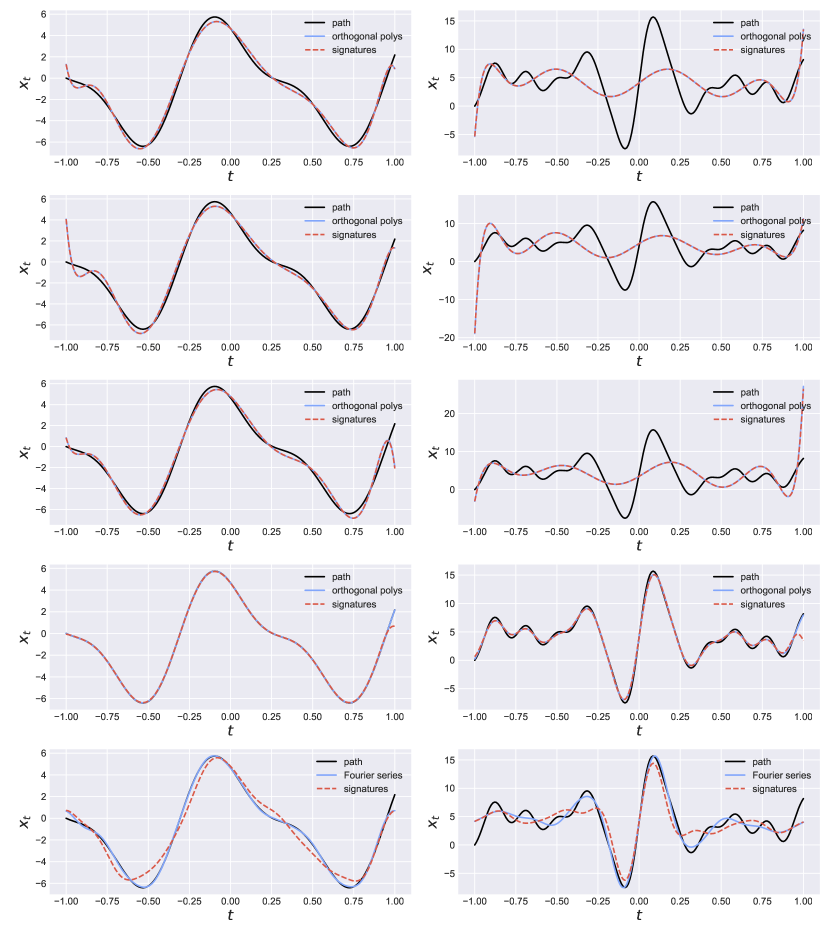
Figure 9: Inversion results for low-frequency and high-frequency example paths, with approximation bases (from top to bottom) Legendre (Jacobi$(0,0)$), Jacobi$(0,0.5)$, Jacobi$(0.5,0))$, Hermite $(\epsilon=0.05)$ and Fourier.

Finally, we provide a brief demonstration of signature inversion on rough paths. Paths are generated from fractional Brownian motion (FBM) [44] with Hurst index $0.5$ and $0.9$. Figure 10 shows the inversion results via different bases on FBM paths. Notably, pointwise inversion via Hermite polynomials captures more subtle changes in the paths, while inversion via Fourier coefficients falls behind in this setting.

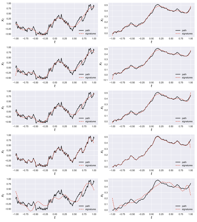
Figure 10: Inversion results on fractional Brownian motion with Hurst $0.5$ and $0.9$, with approximation bases (from top to bottom) Legendre (Jacobi$(0,0)$), Jacobi$(0,0.5)$, Jacobi$(0.5,0)$, Hermite $(\epsilon=0.05)$ and Fourier.

Appendix E Experiment details

In this section, we provide additional details about the experimental setup. We follow the score-based generative diffusion via a variance-preserving SDE paradigm proposed in Song et al. [60]. We tune $\overline{\beta}_{min}$ and $\overline{\beta}_{max}$ in Equation (3) to be 0.1 and 5 respectively. We use a denoising score-matching [66] objective for training the score network $s_{\theta}$. For sampling, we discretize the probability flow ODE derived from Equation (3)

$$d\textbf{x}_{t}=-\frac{1}{2}\beta(t)[\textbf{x}_{t}+s_{\theta}(t,\textbf{x}_{t})]dt,t\in[0,1]$$ (26)

with an initial point $\textbf{x}_{0}\sim\mathcal{N}(0,I)$. To solve the discretized ODE, we use a Tsit5 solver with $128$ time steps. We adopt the implementation of the predictive and discriminative score metrics from TimeGAN [69]. To satisfy the conditions for Fourier inversion, we augment the paths with additional channels as described in Theorem 3.1, and we add an extra point to the beginning of each path, making it start with 0.

The model architecture remains fixed throughout the experiments as a transformer with 4 residual layers, a hidden size of 64, and 4 attention heads. Note that other relevant works [72, 18, 5] follow a very similar or bigger architecture. We use the Adam optimizer. We run the experiments on an NVIDIA GeForce RTX 4070 Ti GPU. Table 4 details the runtime and model sizes.

Table 4: Comparison of model sizes.

Dataset	Model	Parameters	Training Time	Sampling Time
Long sines	SigDiffusion (ours)	229K	8 min	11 sec
	Diffusion-TS	4.18M	57 min	15 min
	CSPD-GP (RNN)	759K	9 min	1 min
	CSPD-GP (Transformer)	973K	15 min	5 min
Predator-prey	SigDiffusion (ours)	211K	8 min	12 sec
	Diffusion-TS	4.17M	55 min	14 min
	CSPD-GP (RNN)	758K	8 min	1 min
	CSPD-GP (Transformer)	972K	16 min	5 min
HEPC	SigDiffusion (ours)	205K	8 min	12 sec
	Diffusion-TS	4.17M	50 min	15 min
	CSPD-GP (RNN)	758K	4 min	1 min
	CSPD-GP (Transformer)	982K	9 min	5 min

For the task of generating time series described in Section 5.2, we fix the number of samples to 1000, the batch size to 128, the number of epochs to 1200, and the learning rate to 0.001. The details variable across datasets are listed in Table 5.

The mirror augmentation

For many datasets, we might not wish to assume path periodicity as required in the Fourier inversion conditions in Theorem 3.1. We observed that a useful trick in this case is to concatenate the path with a reversed version of itself before performing the additional augmentations. We denote this the mirror augmentation. Table 5 indicates the datasets for which this augmentation was performed.

Table 5: Datasets for long time series generation.

Dataset	Mirror augmentation	Data points	Dimensions
Sines	Yes	10000	5
HEPC	No	10242	1
Predator-prey	No	10000	2

Datasets

As previously described in Section 5, we measure the performance of long time series generation on two synthetic (Long sines and Predator-prey) and one real-world (HEPC) dataset, which is under the Open Database (DbCL) license. We generate Long sines the same way the Sine dataset is generated in TimeGAN [70], by sampling sine curves at a random phase and frequency but changing the sampling rate to 1000. Predator-prey is a dataset consisting of sample trajectories of a two-dimensional system of ODEs adopted from [5]

$$\begin{split}\dot{x}=\frac{2}{3}x-\frac{2}{3}xy,\\ \dot{y}=xy-y.\end{split}$$

We generated Predator-prey on a time grid of 1000 points on the interval $t\in[0,10]$. Lastly, HEPC [54] is a household electricity consumption dataset collected minute-wise for 47 months from 2006 to 2010. We slice the dataset to windows of length 1000 with a stride of 200, yielding a dataset of 10242 entries. We select the voltage feature to generate as a univariate time series.

Baselines

We compare our models to three recent diffusion models for long time series generation: Diffusion-TS [72], and two variants of CSPD-GP [5] - one with an RNN for a score function and one with a transformer. We kept the model configurations as they were proposed in the authors’ implementations for datasets with similar dimensions and number of data points. One exception to this is halving the batch size for transformer-based architectures due to memory constraints. We also halved the number of epochs to preserve the proposed number of training steps. Table 4 shows the number of parameters and computation times for each model. We used the publicly available code to run the baselines:

• https://github.com/morganstanley/MSML [62]

• https://github.com/Y-debug-sys/Diffusion-TS [71]

References

- Alaa et al. [2020] Ahmed Alaa, Alex James Chan, and Mihaela van der Schaar. Generative time-series modeling with fourier flows. In International Conference on Learning Representations, 2020.
- Anderson [1982] Brian DO Anderson. Reverse-time diffusion equation models. Stochastic Processes and their Applications, 12(3):313–326, 1982.
- Arribas et al. [2020] Imanol Perez Arribas, Cristopher Salvi, and Lukasz Szpruch. Sig-sdes model for quantitative finance. In Proceedings of the First ACM International Conference on AI in Finance, pages 1–8, 2020.
- Atkinson [2009] Kendall. Atkinson. Theoretical Numerical Analysis A Functional Analysis Framework. Texts in Applied Mathematics, 39. Springer New York, New York, NY, 3rd ed. 2009. edition, 2009. ISBN 1-282-33318-6.
- Biloš et al. [2023] Marin Biloš, Kashif Rasul, Anderson Schneider, Yuriy Nevmyvaka, and Stephan Günnemann. Modeling temporal data as continuous functions with stochastic process diffusion. In International Conference on Machine Learning, pages 2452–2470. PMLR, 2023.
- Buehler et al. [2020] Hans Buehler, Blanka Horvath, Terry Lyons, Imanol Perez Arribas, and Ben Wood. A data-driven market simulator for small data environments. arXiv preprint arXiv:2006.14498, 2020.
- Cai et al. [2020] Ruojin Cai, Guandao Yang, Hadar Averbuch-Elor, Zekun Hao, Serge Belongie, Noah Snavely, and Bharath Hariharan. Learning gradient fields for shape generation. In Computer Vision–ECCV 2020: 16th European Conference, Glasgow, UK, August 23–28, 2020, Proceedings, Part III 16, pages 364–381. Springer, 2020.
- Cass and Salvi [2024] Thomas Cass and Cristopher Salvi. Lecture notes on rough paths and applications to machine learning. arXiv preprint arXiv:2404.06583, 2024.
- Cass and Turner [2024] Thomas Cass and William F Turner. Free probability, path developments and signature kernels as universal scaling limits. arXiv preprint arXiv:2402.12311, 2024.
- Chang and Lyons [2019] Jiawei Chang and Terry Lyons. Insertion algorithm for inverting the signature of a path. arXiv preprint arXiv:1907.08423, 2019.
- Chang et al. [2016] Jiawei Chang, Nick Duffield, Hao Ni, and Weijun Xu. Signature inversion for monotone paths, 2016.
- Chen [1957] Kuo-Tsai Chen. Integration of paths, geometric invariants and a generalized baker-hausdorff formula. Annals of Mathematics, 65(1):163–178, 1957.
- Chen [1958] Kuo-Tsai Chen. Integration of paths–a faithful representation of paths by noncommutative formal power series. Transactions of the American Mathematical Society, 89(2):395–407, 1958.
- Chow [1939] WL Chow. On system of linear partial differential equations of the first order. Mathematische Annalen, 117(1):98–105, 1939.
- Cirone et al. [2023] Nicola Muca Cirone, Maud Lemercier, and Cristopher Salvi. Neural signature kernels as infinite-width-depth-limits of controlled resnets. In International Conference on Machine Learning, pages 25358–25425. PMLR, 2023.
- Cirone et al. [2024] Nicola Muca Cirone, Antonio Orvieto, Benjamin Walker, Cristopher Salvi, and Terry Lyons. Theoretical foundations of deep selective state-space models. arXiv preprint arXiv:2402.19047, 2024.
- Cochrane et al. [2021] Thomas Cochrane, Peter Foster, Varun Chhabra, Maud Lemercier, Terry Lyons, and Cristopher Salvi. Sk-tree: a systematic malware detection algorithm on streaming trees via the signature kernel. In 2021 IEEE international conference on cyber security and resilience (CSR), pages 35–40. IEEE, 2021.
- Coletta et al. [2024] Andrea Coletta, Sriram Gopalakrishnan, Daniel Borrajo, and Svitlana Vyetrenko. On the constrained time-series generation problem. Advances in Neural Information Processing Systems, 36, 2024.
- Diehl et al. [2023] Joscha Diehl, Kurusch Ebrahimi-Fard, and Nikolas Tapia. Generalized iterated-sums signatures. Journal of Algebra, 632:801–824, 2023.
- Dutordoir et al. [2023] Vincent Dutordoir, Alan Saul, Zoubin Ghahramani, and Fergus Simpson. Neural diffusion processes. In International Conference on Machine Learning, pages 8990–9012. PMLR, 2023.
- Esteban et al. [2017] Cristóbal Esteban, Stephanie L Hyland, and Gunnar Rätsch. Real-valued (medical) time series generation with recurrent conditional gans. arXiv preprint arXiv:1706.02633, 2017.
- Fermanian et al. [2023a] Adeline Fermanian, Jiawei Chang, Terry Lyons, and Gérard Biau. The insertion method to invert the signature of a path. arXiv preprint arXiv:2304.01862, 2023a.
- Fermanian et al. [2023b] Adeline Fermanian, Terry Lyons, James Morrill, and Cristopher Salvi. New directions in the applications of rough path theory. IEEE BITS the Information Theory Magazine, 2023b.
- Fliess et al. [1983] Michel Fliess, Moustanir Lamnabhi, and Françoise Lamnabhi-Lagarrigue. An algebraic approach to nonlinear functional expansions. IEEE transactions on circuits and systems, 30(8):554–570, 1983.
- Fons et al. [2022] Elizabeth Fons, Alejandro Sztrajman, Yousef El-Laham, Alexandros Iosifidis, and Svitlana Vyetrenko. Hypertime: Implicit neural representation for time series. arXiv preprint arXiv:2208.05836, 2022.
- Friz and Victoir [2010] Peter K Friz and Nicolas B Victoir. Multidimensional stochastic processes as rough paths: theory and applications, volume 120. Cambridge University Press, 2010.
- Goodfellow et al. [2014] Ian Goodfellow, Jean Pouget-Abadie, Mehdi Mirza, Bing Xu, David Warde-Farley, Sherjil Ozair, Aaron Courville, and Yoshua Bengio. Generative adversarial nets. Advances in neural information processing systems, 27, 2014.
- Ho et al. [2020] Jonathan Ho, Ajay Jain, and Pieter Abbeel. Denoising diffusion probabilistic models. Advances in neural information processing systems, 33:6840–6851, 2020.
- Horvath et al. [2023] Blanka Horvath, Maud Lemercier, Chong Liu, Terry Lyons, and Cristopher Salvi. Optimal stopping via distribution regression: a higher rank signature approach. arXiv preprint arXiv:2304.01479, 2023.
- Hwang et al. [2023] Yechan Hwang, Jinsu Lim, Young-Jun Lee, and Ho-Jin Choi. Augmentation for context in financial numerical reasoning over textual and tabular data with large-scale language model. In NeurIPS 2023 Second Table Representation Learning Workshop, 2023.
- Ismail [2005] Mourad Ismail. Classical and quantum orthogonal polynomials in one variable /. Encyclopedia of mathematics and its applications ; v. 98. Cambridge University Press, Cambridge, 2005. ISBN 9780521782012.
- Issa et al. [2024] Zacharia Issa, Blanka Horvath, Maud Lemercier, and Cristopher Salvi. Non-adversarial training of neural sdes with signature kernel scores. Advances in Neural Information Processing Systems, 36, 2024.
- Jagvaral et al. [2024] Yesukhei Jagvaral, Francois Lanusse, and Rachel Mandelbaum. Unified framework for diffusion generative models in so (3): applications in computer vision and astrophysics. In Proceedings of the AAAI Conference on Artificial Intelligence, volume 38, pages 12754–12762, 2024.
- Jeon et al. [2022] Jinsung Jeon, Jeonghak Kim, Haryong Song, Seunghyeon Cho, and Noseong Park. Gt-gan: General purpose time series synthesis with generative adversarial networks. Advances in Neural Information Processing Systems, 35:36999–37010, 2022.
- Kerrigan et al. [2022] Gavin Kerrigan, Justin Ley, and Padhraic Smyth. Diffusion generative models in infinite dimensions. arXiv preprint arXiv:2212.00886, 2022.
- Kidger et al. [2019] Patrick Kidger, Patric Bonnier, Imanol Perez Arribas, Cristopher Salvi, and Terry Lyons. Deep signature transforms. Advances in Neural Information Processing Systems, 32, 2019.
- Kidger et al. [2020] Patrick Kidger, James Morrill, James Foster, and Terry Lyons. Neural controlled differential equations for irregular time series. Advances in Neural Information Processing Systems, 33:6696–6707, 2020.
- Lemercier et al. [2021a] Maud Lemercier, Cristopher Salvi, Thomas Cass, Edwin V Bonilla, Theodoros Damoulas, and Terry J Lyons. Siggpde: Scaling sparse gaussian processes on sequential data. In International Conference on Machine Learning, pages 6233–6242. PMLR, 2021a.
- Lemercier et al. [2021b] Maud Lemercier, Cristopher Salvi, Theodoros Damoulas, Edwin Bonilla, and Terry Lyons. Distribution regression for sequential data. In International Conference on Artificial Intelligence and Statistics, pages 3754–3762. PMLR, 2021b.
- Lim et al. [2023] Jae Hyun Lim, Nikola B Kovachki, Ricardo Baptista, Christopher Beckham, Kamyar Azizzadenesheli, Jean Kossaifi, Vikram Voleti, Jiaming Song, Karsten Kreis, Jan Kautz, et al. Score-based diffusion models in function space. arXiv preprint arXiv:2302.07400, 2023.
- Lyons [1998] Terry J Lyons. Differential equations driven by rough signals. Revista Matemática Iberoamericana, 14(2):215–310, 1998.
- Lyons and Xu [2017] Terry J Lyons and Weijun Xu. Hyperbolic development and inversion of signature. Journal of Functional Analysis, 272(7):2933–2955, 2017.
- Lyons and Xu [2018] Terry J Lyons and Weijun Xu. Inverting the signature of a path. Journal of the European Mathematical Society, 20(7):1655–1687, 2018.
- Mandelbrot and Van Ness [1968] Benoit B Mandelbrot and John W Van Ness. Fractional brownian motions, fractional noises and applications. SIAM review, 10(4):422–437, 1968.
- Manten et al. [2024] Georg Manten, Cecilia Casolo, Emilio Ferrucci, Søren Wengel Mogensen, Cristopher Salvi, and Niki Kilbertus. Signature kernel conditional independence tests in causal discovery for stochastic processes. arXiv preprint arXiv:2402.18477, 2024.
- Mogren [2016] Olof Mogren. C-rnn-gan: Continuous recurrent neural networks with adversarial training. arXiv preprint arXiv:1611.09904, 2016.
- Morrill et al. [2021] James Morrill, Cristopher Salvi, Patrick Kidger, and James Foster. Neural rough differential equations for long time series. In International Conference on Machine Learning, pages 7829–7838. PMLR, 2021.
- Pannier and Salvi [2024] Alexandre Pannier and Cristopher Salvi. A path-dependent pde solver based on signature kernels. arXiv preprint arXiv:2403.11738, 2024.
- Pei et al. [2021] Hengzhi Pei, Kan Ren, Yuqing Yang, Chang Liu, Tao Qin, and Dongsheng Li. Towards generating real-world time series data. In 2021 IEEE International Conference on Data Mining (ICDM), pages 469–478. IEEE, 2021.
- Phillips et al. [2022] Angus Phillips, Thomas Seror, Michael Hutchinson, Valentin De Bortoli, Arnaud Doucet, and Emile Mathieu. Spectral diffusion processes. arXiv preprint arXiv:2209.14125, 2022.
- Popov et al. [2021] Vadim Popov, Ivan Vovk, Vladimir Gogoryan, Tasnima Sadekova, and Mikhail Kudinov. Grad-tts: A diffusion probabilistic model for text-to-speech. In International Conference on Machine Learning, pages 8599–8608. PMLR, 2021.
- Ree [1958] Rimhak Ree. Lie elements and an algebra associated with shuffles. Annals of Mathematics, 68(2):210–220, 1958.
- Reizenstein [2017] Jeremy Reizenstein. Calculation of iterated-integral signatures and log signatures. arXiv preprint arXiv:1712.02757, 2017.
- Repository [2024] UCI Machine Learning Repository. Electric power consumption dataset. https://www.kaggle.com/datasets/uciml/electric-power-consumption-data-set, 2024. Accessed: 2024-05-21.
- Reutenauer [2003] Christophe Reutenauer. Free lie algebras. In Handbook of algebra, volume 3, pages 887–903. Elsevier, 2003.
- Rubanova et al. [2019] Yulia Rubanova, Ricky TQ Chen, and David K Duvenaud. Latent ordinary differential equations for irregularly-sampled time series. Advances in neural information processing systems, 32, 2019.
- Salvi et al. [2021a] Cristopher Salvi, Thomas Cass, James Foster, Terry Lyons, and Weixin Yang. The signature kernel is the solution of a goursat pde. SIAM Journal on Mathematics of Data Science, 3(3):873–899, 2021a.
- Salvi et al. [2021b] Cristopher Salvi, Maud Lemercier, Chong Liu, Blanka Horvath, Theodoros Damoulas, and Terry Lyons. Higher order kernel mean embeddings to capture filtrations of stochastic processes. Advances in Neural Information Processing Systems, 34:16635–16647, 2021b.
- Salvi et al. [2023] Cristopher Salvi, Joscha Diehl, Terry Lyons, Rosa Preiss, and Jeremy Reizenstein. A structure theorem for streamed information. Journal of Algebra, 634:911–938, 2023.
- Song and Ermon [2019] Yang Song and Stefano Ermon. Generative modeling by estimating gradients of the data distribution. Advances in neural information processing systems, 32, 2019.
- Song et al. [2020] Yang Song, Jascha Sohl-Dickstein, Diederik P Kingma, Abhishek Kumar, Stefano Ermon, and Ben Poole. Score-based generative modeling through stochastic differential equations. arXiv preprint arXiv:2011.13456, 2020.
- Stanley [2024] Morgan Stanley. Msml: Morgan stanley machine learning. https://github.com/morganstanley/MSML, 2024. Accessed: 2024-05-21.
- Tashiro et al. [2021] Yusuke Tashiro, Jiaming Song, Yang Song, and Stefano Ermon. Csdi: Conditional score-based diffusion models for probabilistic time series imputation. Advances in Neural Information Processing Systems, 34:24804–24816, 2021.
- Trottet et al. [2023] Cécile Trottet, Manuel Schürch, Amina Mollaysa, Ahmed Allam, and Michael Krauthammer. Generative time series models with interpretable latent processes for complex disease trajectories. In Deep Generative Models for Health Workshop NeurIPS 2023, 2023.
- Vaswani et al. [2017] Ashish Vaswani, Noam Shazeer, Niki Parmar, Jakob Uszkoreit, Llion Jones, Aidan N Gomez, Łukasz Kaiser, and Illia Polosukhin. Attention is all you need. Advances in neural information processing systems, 30, 2017.
- Vincent [2011] Pascal Vincent. A connection between score matching and denoising autoencoders. Neural computation, 23(7):1661–1674, 2011.
- Voleti et al. [2022] Vikram Voleti, Alexia Jolicoeur-Martineau, and Chris Pal. Mcvd-masked conditional video diffusion for prediction, generation, and interpolation. Advances in neural information processing systems, 35:23371–23385, 2022.
- Yildiz et al. [2019] Cagatay Yildiz, Markus Heinonen, and Harri Lahdesmaki. Ode2vae: Deep generative second order odes with bayesian neural networks. Advances in Neural Information Processing Systems, 32, 2019.
- Yoon [2024] Jinsung Yoon. Timegan: Temporal generative adversarial networks for time-series synthesis - main script. https://github.com/jsyoon0823/TimeGAN/blob/master/main_timegan.py, 2024. Accessed: 2024-05-21.
- Yoon et al. [2019] Jinsung Yoon, Daniel Jarrett, and Mihaela Van der Schaar. Time-series generative adversarial networks. Advances in neural information processing systems, 32, 2019.
- Yuan [2024] Xinyu Yuan. Diffusion-ts: Diffusion models for time series. https://github.com/Y-debug-sys/Diffusion-TS, 2024. Accessed: 2024-05-21.
- Yuan and Qiao [2024] Xinyu Yuan and Yan Qiao. Diffusion-ts: Interpretable diffusion for general time series generation. arXiv preprint arXiv:2403.01742, 2024.
- Zhou et al. [2023] Linqi Zhou, Michael Poli, Winnie Xu, Stefano Massaroli, and Stefano Ermon. Deep latent state space models for time-series generation. In International Conference on Machine Learning, pages 42625–42643. PMLR, 2023.