Phases and phase transition in Grover’s algorithm with systematic noise

Abstract

While limitations on quantum computation by Markovian environmental noise are well-understood in generality, their behavior for different quantum circuits and noise realizations can be less universal. Here we consider a canonical quantum algorithm - Grover’s algorithm for unordered search on $L$ qubits - in the presence of systematic noise. This allows us to write the behavior as a random Floquet unitary, which we show is well-characterized by random matrix theory (RMT). The RMT analysis enables analytical predictions for phases and phase transitions of the many-body dynamics. We find two separate transitions. At moderate disorder $\delta_{c,\mathrm{gap}}\sim L^{-1}$, there is a ergodicity breaking transition such that a finite-dimensional manifold remains non-ergodic for $\delta<\delta_{c,\mathrm{gap}}$. Computational power is lost at a much smaller disorder, $\delta_{c,\mathrm{comp}}\sim L^{-1/2}2^{-L/2}$. We comment on relevance to non-systematic noise in realistic quantum computers, including cold atom, trapped ion, and superconducting platforms.

I Introduction

Significant progress has been made in the last few years toward building noisy intermediate scale quantum (NISQ) computers [1]. These quantum devices have fewer qubits ranging from dozens to a few hundred and despite their limitations, they have been used to tackle certain classically challenging problems and emulate numerous many-body phases of matter [2, 3]. However, more conventional quantum algorithms designed for ideal quantum computers do not in general perform meaningful computations when run on a NISQ device, suggesting that general usage will require quantum error correction.

Until such a time as quantum error correction is achieved, it remains important to understand the role of noise in creating issues for known quantum algorithms. One such algorithm is Grover’s algorithm for unstructured database search [4]. It has been the subject of intense study and has, in fact, been implemented on various NISQ devices [5, 6, 7]. The effects of noise on Grover’s search has been studied using different models and efforts have been made towards putting limits on the performance of the algorithm. For example, Long et al. [8] determined that the size of the database is constrained by $\mathcal{O}(1/\delta^{2})$ where $\delta$ is an error parameter representing gate imperfection. In the presence of random phase error in the oracle gate, Shenvi et al. [9] have shown that in order to maintain the probability of success, the error must decrease as $k^{1/4}$ when the database size is increased by a factor of $k$. In case of depolarizing noise channel, Salas [10] found that the noise threshold behaves as $N^{-1.1}$, where $N$ is the size of the database. Norman and Ataba [11] determined that the allowed noise rate scales as $N^{-2/3}$ if Gaussian noise is added at each step of the algorithm. Finally, Shapira et al. [12] showed that in case of unitary noise characterized by standard deviation $\epsilon$, must satisfy $\epsilon<\mathcal{O}(L^{-1/2}N^{-1/4})$ where $N=2^{L}$, in order for the algorithm to maintain a significant efficiency.

These cases primarily studied aphysical noise models on the long-range many-qubit Grover gates and consistently found that exponentially small error rates prevent the algorithm from succeeding. These error models make generalizing the results rather challenging, leaving open the question whether other physically realistic error models might have improved performance bounds. Furthermore, the standard Grover algorithm involves a call to an oracle which is a non-$k$-local operation that is aphysical in most realizations. We will consider the impact of errors on a circuit in which the oracle is unraveled into $k$-local unitary gates (cf. Figure 2), which comes at the cost of larger depth.

In order to get a better analytical handle on the error-tolerance of Grover’s algorithm, we consider here the effects of systematic gate noise, i.e., undesired noise in the quantum gates that is repeated systematically throughout the course of the algorithm. Systematic noise naturally occurs in most experiments due to calibration issues. For our purposes, it imbues the noisy algorithm with a time-periodic (Floquet) structure, such that we can find exact scaling of target state dynamics, noise thresholds, and other physically relevant quantities by employing both analytical and numerical approaches. We show that these signatures can be captured by a simple random-matrix Hamiltonian whose perturbative effect on the Floquet spectrum describes gap-closing transitions that determine the response to noise. We find that for a database of size $N=2^{L}$, the algorithm loses its computational power at a noise strength that scales as $L^{-1/2}N^{-1/2}$. Additionally, an ergodicity transition occurs at a noise strength that scales as $1/L$ with the system size. Using state-of-the-art numerics, we show that these analytical predictions align perfectly with the exact numerical solution and comment on the relevance to using Grover’s algorithm – as well as related amplitude amplification techniques – in the NISQ era.

II Model

We start by reviewing the basic formulation of Grover’s algorithm. Suppose we want to search for an item $w$ in an unstructured database with $N=2^{L}$ items. For simplicity, let us assume that the target item $w$ is unique. The search problem can be expressed by using an indicator function $f(x)$ that takes integer inputs $x$, with $0\leq x\leq N-1$, such that

$$f(x)=\begin{cases}1&\text{if $x$ is a solution, i.e., $x=w$}\\ 0&\text{otherwise.}\end{cases}$$ (1)

In case of Grover’s algorithm, this indicator function is implemented using a unitary operator $U_{w}$, known as the oracle, whose action on the computational basis states is

$$|x\rangle\xrightarrow{U_{w}}(-1)^{f(x)}|x\rangle.$$ (2)

The complexity of an algorithm can be measured by the number of times the function $f(x)$ is evaluated. Classical algorithms require $\sim N/2$ “time steps” – calls to a circuit that evaluates the function $f(x)$ – on average to find the target state. Grover’s algorithm requires $\mathcal{O}(\sqrt{N})$ evaluations of the oracle $O$ to obtain the target state, and thus provides quadratic advantage over the classical counterparts.

Instead of the elements of the database directly, Grover’s algorithm focuses on the indices of the elements, such that the database can be represented using $L$ qubits as $\{|0\rangle,|1\rangle,\cdots,|2^{L}-1\rangle\}$. The algorithm starts with the uniform superposition state $|x\rangle=\frac{1}{\sqrt{N}}\sum^{N-1}_{j=0}|j\rangle$, and then amplifies the amplitude of the target state $|w\rangle$ using the action of the two unitary operators. First it applies the oracle, which flips the sign of the state $|w\rangle$,

$$U_{w}|k\rangle=(2|w\rangle\langle w|-I)|k\rangle=\begin{cases}|k\rangle&\text{if }k=w\\ -|k\rangle&\text{if }k\neq w\end{cases}.$$ (3)

Second is the “diffusion” operator $U_{x}$, which flips the amplitude of all the states about their mean,

$$U_{x}\sum_{k}\alpha_{k}|k\rangle = (2|x\rangle\langle x|-I)\sum_{k}\alpha_{k}|k\rangle,$$ (4)

$$= \sum_{k}(-\alpha_{k}+\sum_{j}\alpha_{j}/N)|k\rangle.$$

The combined action of these two reflections are written in terms of the Grover operator as $G_{w}=U_{x}U_{w}$, which gradually rotates the initial state $|x\rangle$ towards the target state $|w\rangle$. The action of $G_{w}$ on the state of the system can be interpreted geometrically by writing the state of the system at $t=0$ as

$$|\psi(t=0)\rangle=|x\rangle =\cos\theta|\bar{x}(w)\rangle+\sin\theta|w\rangle,$$ (5)

$$\mbox{where}\hskip 14.22636pt|\bar{x}(w)\rangle =\frac{1}{\sqrt{N-1}}\sum_{j\neq w}|j\rangle,$$ (6)

and $\sin\theta=1/\sqrt{N}$ . Then the state of the system at time $t$ can be written as

$$|\psi(t)\rangle = (G_{w})^{t}|\psi(t=0)\rangle,$$ (7)

$$=\cos[(2t+1)\theta]|\bar{x}(w)\rangle+\sin[(2t+1)\theta]|w\rangle.$$

In other words, $G_{w}$ rotates the wave function in the two dimensional subspace spanned by $|\bar{x}_{w}\rangle$ and $|w\rangle$ by angle $2\theta$. From Eq. (7), we get the probability of measuring the target $|w\rangle$ after $t$ steps as,

$$P_{w}(t)=\sin^{2}[(2t+1)\theta].$$ (8)

Therefore, to obtain the target state with maximum probability, one performs a measurement on the system at $t=\lfloor\frac{\pi}{4}\sqrt{N}\rfloor$ steps [13]. Not only does this scale faster than a classical computer; it has in fact been shown that Grover’s algorithm is asymptotically optimal on an ideal quantum computer [14].

II.1 Floquet spectrum

Since Grover’s algorithm involves the repeated application of an identical unitary $G_{w}$, it can be achieved by an appropriately chosen time-periodic Hamiltonian $H(t+T)=H(t)$. In other words, Grover’s algorithm is an example of a Floquet problem [15]. This allows us to define the time-independent Floquet Hamiltonian $H_{F}$ as [16, 17]

$$G_{w}=\mathcal{T}e^{-i\int^{T}_{0}dtH(t)}=e^{-iH_{F}T},$$ (9)

where we choose units with $\hbar=1$ throughout. It follows that eigenstates $|u_{\alpha}\rangle$ of $G_{w}$ satisfy

$$G_{w}|u_{\alpha}\rangle=e^{-i\phi_{\alpha}T}|u_{\alpha}\rangle.$$ (10)

The quasi-energies $\phi_{\alpha}$ are defined modulo $2\pi/T$, where period $T\equiv 1$ represents the time required to apply $G_{w}$ on the qubits.

Before we write down the exact eigenstates and quasi-energies for the Grover operator, we state a useful theorem that simplifies our analysis: the spectrum of the Grover operator is independent of the target state $w$. To prove this, consider conjugation by the unitary matrix

$$V_{w}=\prod_{j\in w}X_{j}=V_{w}^{\dagger},$$ (11)

where the notation $j\in w$ indicates to take a product over Pauli $X$ operators only acting on sites where $w$ is in state $1$. Then

$$V_{w}G_{w}V_{w}^{\dagger} = G_{0}.$$ (12)

Since $G_{0}$ and $G_{w}$ are unitarily equivalent, their eigenvalues are identical. We will therefore focus on target state $w=0$ (state $|0\rangle$ on all qubits) for the remainder of the work.

The Grover operator $G_{0}$ has two eigenstates with non-zero quasi-energies, which we will refer to as the special states,

$$G_{0}\frac{1}{\sqrt{2}}(|0\rangle\pm i|\bar{x}\rangle) = [\frac{2}{N}-1\mp i\frac{2\sqrt{N-1}}{N}]\frac{1}{\sqrt{2}}(|0\rangle\pm i|\bar{x}\rangle)$$ (13)

$$= e^{-i\phi_{F\pm}}\frac{1}{\sqrt{2}}(|0\rangle\pm i|\bar{x}\rangle),$$

where

$$\phi_{F_{\pm}}=-\pi\mp\arctan\left(\frac{2\sqrt{N-1}}{N-2}\right)=-\pi\mp 2\theta,$$ (14)

and

$$|\bar{x}\rangle\equiv|\bar{x}(w=0)\rangle=\frac{1}{\sqrt{N-1}}\sum^{N-1}_{j=1}|j\rangle.$$ (15)

The rest of the eigenstates, which we will refer to as the bulk states, are all degenerate at zero quasi-energy,

$$G_{0}|\bar{x}_{n}\rangle=|\bar{x}_{n}\rangle.$$ (16)

Noting that $|\bar{x}\rangle$ is a “zero-momentum” superposition of the non-target states, we choose the following basis for the degenerate bulk subspace:

$$|\bar{x}_{n}\rangle=\frac{1}{\sqrt{N-1}}\sum_{j=1}^{N-1}e^{i(j-1)k_{n}}|j\rangle,$$ (17)

where $k_{n}=(2\pi n)/(N-1)$, and $n=1,2,\cdots,N-2$. In the absence of noise, these states are gapped out and decoupled from the dynamics.

II.2 Gate decomposition

For any practical realization of Grover’s algorithm, the Grover operator $G_{0}$ must be decomposed into one- and two-qubit gates. This can be done for any unitary operator with an appropriate universal set of quantum gates [18], but the decomposition is not unique. Therefore, choosing an efficient gate decomposition will be crucial to the performance of algorithm upon adding noise.

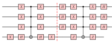
Figure 1: Circuit for the four qubit Grover operator $G_{0}$.

In Figure 1, the quantum circuit for Grover’s operator $G_{0}$ for four qubits is shown. The oracle and the Grover’s diffusion operators are written in terms of a multi-controlled $X$, a.k.a. $L-$qubit Toffoli, gate for ease of decomposition, as such gates are more commonly studied in the literature than the desired multi-controlled $Z$ gate. Decomposing the $L$–qubit Toffoli can be done many different ways, such as using automated transpilation methods (e.g. ‘transpile’ in Qiskit) or via the general algorithm described in the classic paper by Barenco et al. [19]. However, these decompositions result in a circuits whose depth scales non-optimally with system size; it appears to scale exponentially with $L$ using Qiskit transpilation and is known to scale as $L^{2}$ using the Barenco algorithm. In anticipation of improving performance on the noisy algorithm, we instead use the linear depth decomposition algorithm described in [20]. For a multi-controlled $X$ gate with $L$ qubits, this algorithm provides a decomposition with circuit depth $8L-20$ and with $2L^{2}-6L+5$ controlled $x$-rotation gates, hereafter denoted by $CR_{x}(\theta)$. An example for the case of $L=4$ is shown in Figure 2. Note that, while the depth is linear, it relies on the ability to perform multiple finite-range control gates in parallel that share the same control qubit. If these gates cannot be parallelized, the results below will be unchanged, but any realistic quantum computer that includes non-unitary noise ($T_{1}$, $T_{2}$, etc.) will have its performance degraded. Note also that here a single Floquet unitary already has extensive depth $\sim L$, as opposed to more conventional Floquet operators whose depth is usually $L$-independent.

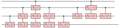
Figure 2: Example decomposition of the four-qubit-controlled $X$ gate in Figure 1 in linear depth using the algorithm described in [20]. The gates with same control qubit are shown together.

II.3 Systematic noise

We consider a systematic noise model with random under or over rotation of each single or two-qubit quantum gate,

$$U_{k}(\theta_{k})\to U_{k}(\theta_{k}+\delta\epsilon_{k}),$$ (18)

where the index $k$ refers to the $k^{th}$ gate in the decomposition of the Grover operator, $\epsilon_{k}$ is drawn from the uniform distribution $[-1,1]$ and $\delta$ is the noise strength. Importantly, each Floquet cycle has an identical noise configuration, so that the operator $G_{w}$ is identical across time steps. This ensures that each iteration of the Grover algorithm is a (random) Floquet problem.

To implement this systematic noise model for our one-qubit gates, we start from unitaries of the form $U_{k}(0)\equiv\sigma_{k}\in\{X,Z,H\}$ which represent single-qubit $\pi$ rotations around the $\hat{x}$, $\hat{z}$, and $(\hat{x}+\hat{z})/\sqrt{2}$ axes, respectively. We can write this as

$$U_{k}(0)=R_{\sigma_{k}}(\pi),\mbox{ where }R_{\sigma_{k}}(\theta)=\exp\{-\frac{i\theta}{2}(I-\sigma_{k})\}$$ (19)

represents a rotation by angle $\theta$ about the $\sigma_{k}$ axis. Then we define the noisy gates as a random over/under-rotation,

$$U_{k}(\delta\epsilon_{k})=R_{\sigma_{k}}(\pi+2\delta\epsilon_{k}).$$ (20)

Similarly, we write the noisy two-qubit controlled rotations as

$$CR_{x}(\theta_{k}+\delta\epsilon_{k})=|0\rangle\langle 0|_{c}\otimes I_{t}+|1\rangle\langle 1|_{c}\otimes R_{x}(\theta_{k}+\delta\epsilon_{k})_{t}$$ (21)

where the convention is chosen such that $CR_{x}(\pi)=|0\rangle\langle 0|_{c}\otimes I_{t}+|1\rangle\langle 1|_{c}\otimes X_{t}$. Note that an identical noise amplitude is added to each control gate independent of the magnitude of the desired rotation $\theta_{k}$. For small $\theta_{k}\lesssim\delta$, this means that the gate is predominately noise, suggesting that further improvements can be made by simply neglecting gates that fall below this threshold. Doing so would complicate the analysis below, but will be worth investigating in future research.

III Results

III.1 Spectrum of noisy Grover operator

To begin exploring the effect of system noise on the performance of the algorithm, we numerically calculate the Floquet quasi-energies and eigenstates of the Grover operator in presence of systematic noise. To probe thermalization of the bulk states, we calculate the bipartite von Neumann entanglement entropy $S_{A}$ of each eigenstate. We choose a subsystem $A$ of $L/2$ consecutive qubits (with periodic boundary conditions) and calculate the entropy $S_{A}=-\text{Tr}(\rho_{A}\ln\rho_{A})$, where $\rho_{A}=\text{Tr}_{\bar{A}}(|\psi\rangle\langle\psi|)$ is the reduced density matrix in eigenstate $|\psi\rangle$. For each eigenstate, the entanglement entropy is averaged over the $L/2$ independent choices of subsystem $A$ .

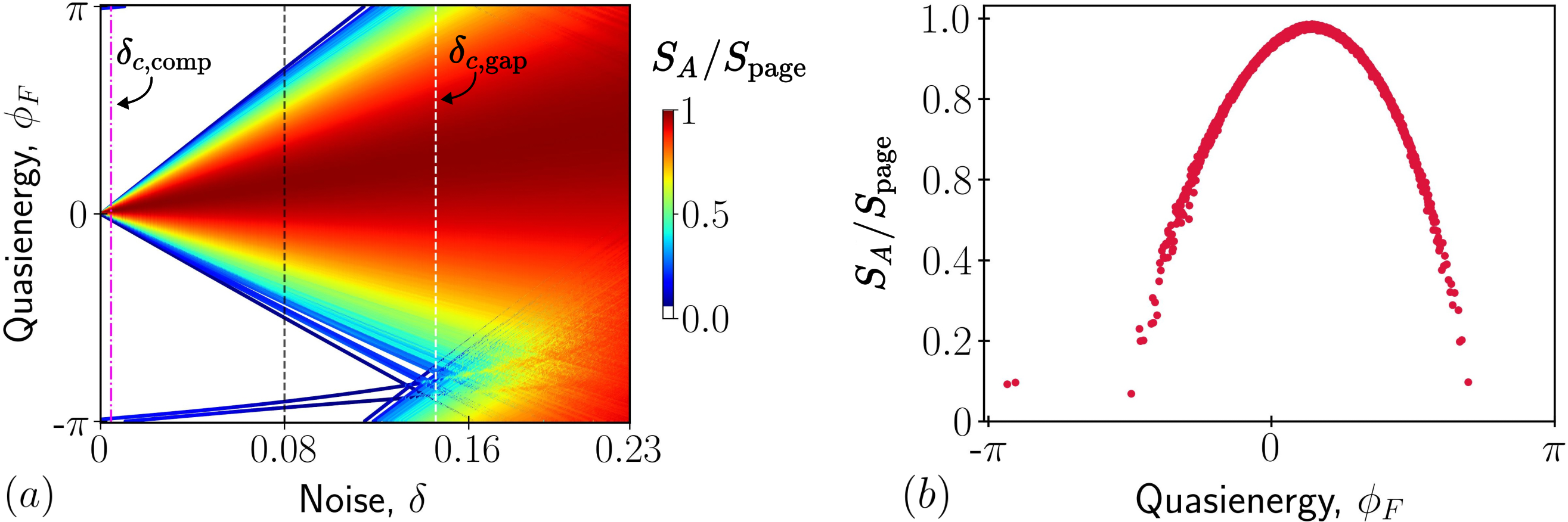
Figure 3: (a) Quasienergies $(\phi_{F})$ of the Grover operator as a function of noise strength $(\delta)$ for $L=12$. The colorbar represents the average bipartite von Neumann entanglement entropy $S_{A}$ normalized by its Page value [22], $S_{\rm Page}=3.66$ for $L=12$. The data is shown for a single realization of systematic noise $\{\epsilon_{k}\}$, which is kept constant for different $\delta$ values. The two critical noise values $\delta_{c,\mathrm{comp}}$ and $\delta_{c,\mathrm{gap}}$ are shown with vertical lines.(b) Entanglement entropy of the bulk quasienergies at noise strength $\delta=0.08$.

An example of the quasi-energies and their entanglement entropies are shown for a single noise realization in Figure 3. The bulk quasi-energies have their degeneracy broken by the noise. Moreover, these bulk states show clear linear dependence on the noise strength $\delta$, which comes from the exponential degeneracy of the unperturbed spectrum. This suggests that the bulk properties are well-described by first-order perturbation theory, even at relatively large $\delta$, which we use in the next section to derive an effective Hamiltonian for the quasi-energy spectrum. Because the bulk spectrum remains far from the edge of the Floquet Brillouin zone at $\pi$ quasienergy, the effective Hamiltonian is time-independent despite coming from a Floquet problem.

In addition to this linear $\delta$-dependence of quasi-energy, the bulk eigenstates show entanglement characteristic of a thermal quantum system, where they should match the thermal entropy $S(E)$. The entanglement peaks in the middle of the bulk spectrum at approximately its maximum value $S_{\mathrm{Page}}=\left[L\ln(2)-1\right]/2$ [22]. As expected, the entropy density approaches zero at either edge of the bulk spectrum. Further evidence for thermalizing (random matrix) behavior will be given in Section III.2.1.

Finally, below some critical value of noise strength $\delta<\delta_{c,\rm gap}$, the special states remain gapped from the bulk. Since Grover’s algorithm involves coherent oscillations within the special state manifold, this suggests that there is a “computing” phase at small $\delta$ where finite probability of finding the target state will survive the systematic noise. We will indeed show that this is true at small enough $\delta$ though, as we will see in our analysis of the special states (Section III.4), the computing transition happens at a much smaller critical value $\delta_{c,\rm comp}\ll\delta_{c,\rm gap}$. Anticipating the results that we are about to show, $\delta_{c,\rm gap}$ will in fact correspond to an ergodicity transition; for $\delta<\delta_{c,\mathrm{gap}}$, initial states within the special state manifold do not thermalize at late time, while for $\delta>\delta_{c,\mathrm{gap}}$, all states thermalize to infinite temperature.

III.2 Effective Hamiltonian of the bulk

We start by using our observation of clear linear $\delta$-dependence of the bulk spectrum to derive an effective Hamiltonian from first order degenerate perturbation theory. To achieve this goal, let us begin by writing the Grover operator with noise strength $\delta$ as

$$G(\delta)=e^{-iH_{M}(\theta_{M}+\delta\epsilon_{M})}\cdots e^{-iH_{1}(\theta_{1}+\delta\epsilon_{1})},$$ (22)

where we have written each gate in the decomposition of the Grover operator as generalized rotations in Hilbert space (see Eq. (20)). Here $M=4L^{2}-6L+10$ is the total number of gates in the decomposition of the $L$-qubit Grover operator. Individual commuting gates are divided into separate terms in the product. Expanding the exponentials and keeping terms only up to first order in $\delta$, we obtain

$$G(\delta) \approx e^{-iH_{M}\theta_{M}}(1-i\delta\epsilon_{M}H_{M})\cdots e^{-iH_{1}\theta_{1}}(1-i\delta\epsilon_{1}H_{1})$$ (23)

$$\approx (1-i\delta H_{\rm eff})G_{0},$$

where we have defined the effective Hamiltonian as

$$H_{\rm eff}=\sum_{k=1}^{M}\epsilon_{k}e^{-iH_{M}\theta_{M}}e^{-iH_{M-1}\theta_{M-1}}\cdots e^{-iH_{k+1}\theta_{k+1}}H_{k}e^{iH_{k+1}\theta_{k+1}}\cdots e^{iH_{M-1}\theta_{M-1}}e^{iH_{M}\theta_{M}}.$$ (24)

We identify $H_{\rm eff}$ as the generator of gate perturbations in the Heisenberg picture . To demonstrate that $H_{\rm eff}$ correctly describes the exact bulk quasienergies, let us consider the action of $G(\delta)$ on these eigenstates. Using Eq. (16), and keeping terms within the first order in $\delta$, we get

$$G(\delta)|\bar{x}_{n\neq 0}\rangle \approx (1-i\delta H_{\rm eff})G_{0}|\bar{x}_{n\neq 0}\rangle,$$ (25)

$$= (1-i\delta H_{\rm eff})|\bar{x}_{n\neq 0}\rangle,$$

$$\approx e^{-i\delta H_{\rm eff}}|\bar{x}_{n\neq 0}\rangle$$

Thus, after discarding the two special states from $H_{\rm eff}$, its eigenvalues should match with the exact bulk quasienergies of $G(\delta)$. In Figure 4, we plot the noise-averaged difference between the exact and the effective energies:

$$d\left(\frac{\phi_{\rm exact}}{\delta},E_{\rm eff}\right)\equiv\left[\sum_{k\in\rm bulk}\left(\frac{\phi_{\rm exact,k}}{\delta}-E_{\rm eff,k}\right)^{2}\right]^{1/2}$$ (26)

as a function of noise strength $\delta$. We see that deviations vanish linearly as $\delta\to 0$ , confirming the correctness of first-order perturbation theory. Indeed, we numerically see that first-order perturbation accurately captures the spectrum nearly up to the value of $\delta$ when the bulk spans the entire Floquet Brillouin zone from $-\pi$ to $\pi$.

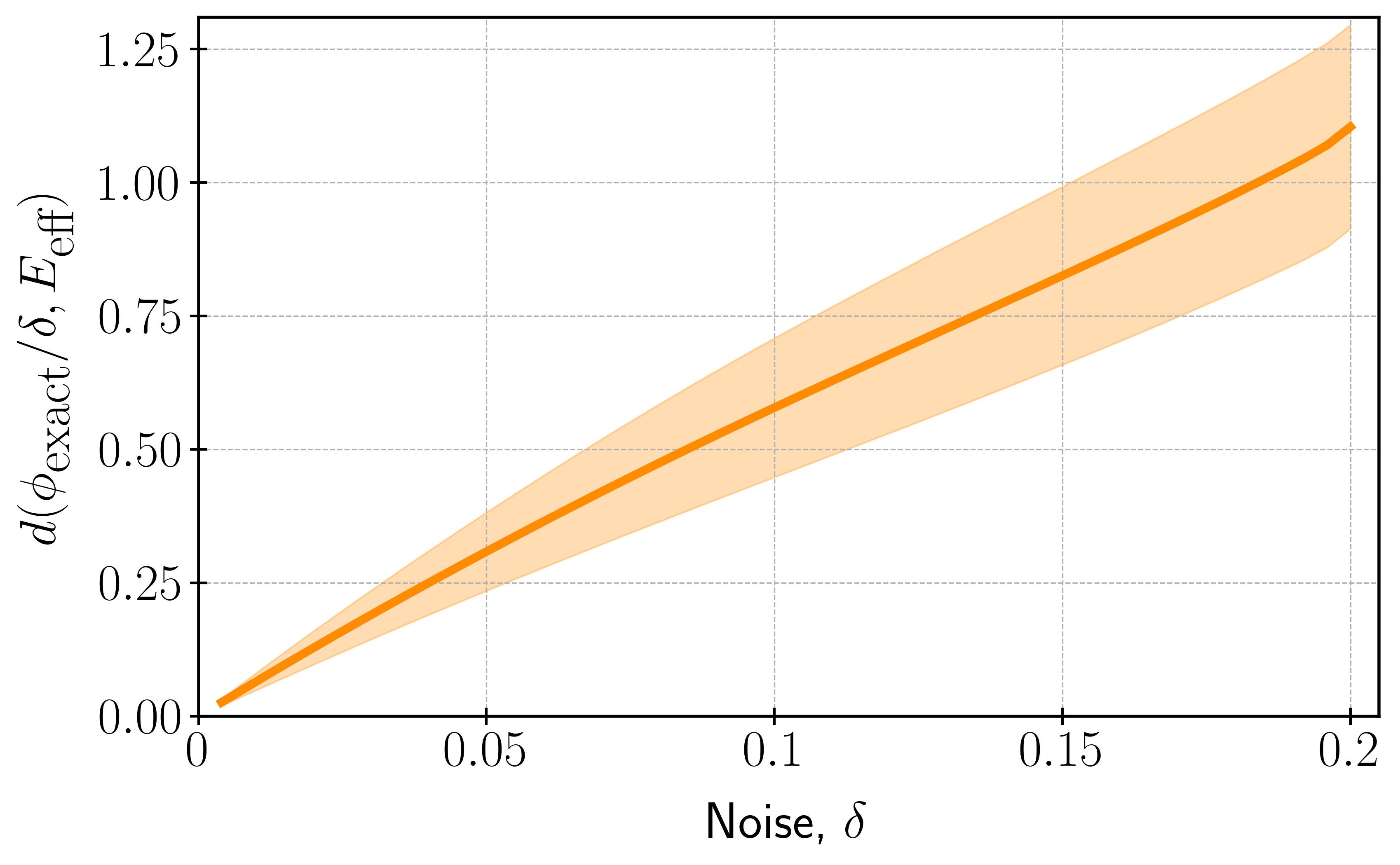
Figure 4: Plot of noise averaged difference between the exact quasi-energy of $G(\delta)$ and eigenvalues of $\delta H_{\rm eff}$ for $L=8$ using Eq. (26). Error bands represents the standard error of mean for five noise realizations.

It is worth noting that our effective Hamiltonian is defined to be independent of the scaling parameter $\delta$, which allows us to analyze the statistical properties of $H_{\rm eff}$ for different noise strengths and therefore determine many important properties such as thermalization of the bulk states and scaling of $\delta_{c,\rm gap}$. Having shown the accuracy of $H_{\rm eff}$ in modeling our spectrum, we now turn to analyzing its properties with a focus on the bulk states. $H_{\rm eff}$ consists of random terms which start as 2-local terms before Heisenberg evolution causes operator spreading. Some remnant of the locality remains, as we argue numerically in the appendix (Section A). However, lacking any other structure, we would expect this Hamiltonian to exhibit generic, thermalizing behavior. We now show this by numerically demostrating its consistency with random matrix theory.

III.2.1 Random matrix theory treatment of $H_{\mathrm{eff}}$

In the thermal phase, the energy levels of a many-body Hamiltonian show level repulsion, and their statistics follow that of a random matrix, the underlying ensemble of which depends on the symmetries of the Hamiltonian in the problem. Here, we examine two properties of $H_{\mathrm{eff}}$ to demonstrate signatures of random matrix theory (RMT). First, to indicate the existence and amount of level repulsion (which is characteristic of the RM ensemble), we examine the level spacing ratio $r_{n}=\text{min}(\Delta E_{n},\Delta E_{n+1})/\text{max}(\Delta E_{n},\Delta E_{n+1})$, where $\Delta E_{n}=E_{n}-E_{n-1}$ is difference between the ordered eigenenergies of $H_{\rm eff}$ [24]. Second, to study the ergodic structure of the eigenstates, we calculate the Kullback-Leibler (KL) divergence (also called the relative entropy) in the computational basis. It is defined as $\text{KLd}_{n}=\sum_{i=1}^{dim\mathcal{H}}p_{i}\ln(p_{i}/q_{i})$, where $p_{i}=|\langle i|n\rangle|^{2}$ and $q_{i}=|\langle i|n+1\rangle|^{2}$ are the occupation probabilities of two energetically-neighboring eigenstates $|n\rangle$ and $|n+1\rangle$ in the $Z$ (computational) basis $\{|i\rangle\}$ [25, 26]. To calculate these two metrics, we sample $H_{\rm eff}$ for different noise realizations, and calculate the level spacing ratio and KL divergence for each, and then average over noise realizations.

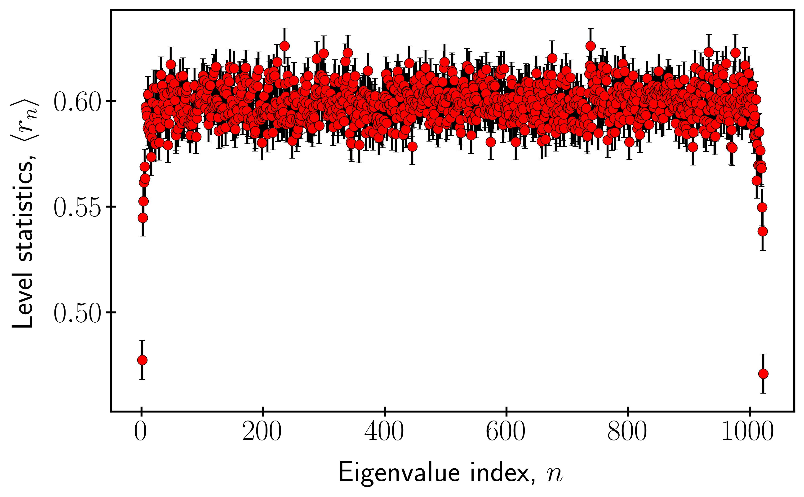
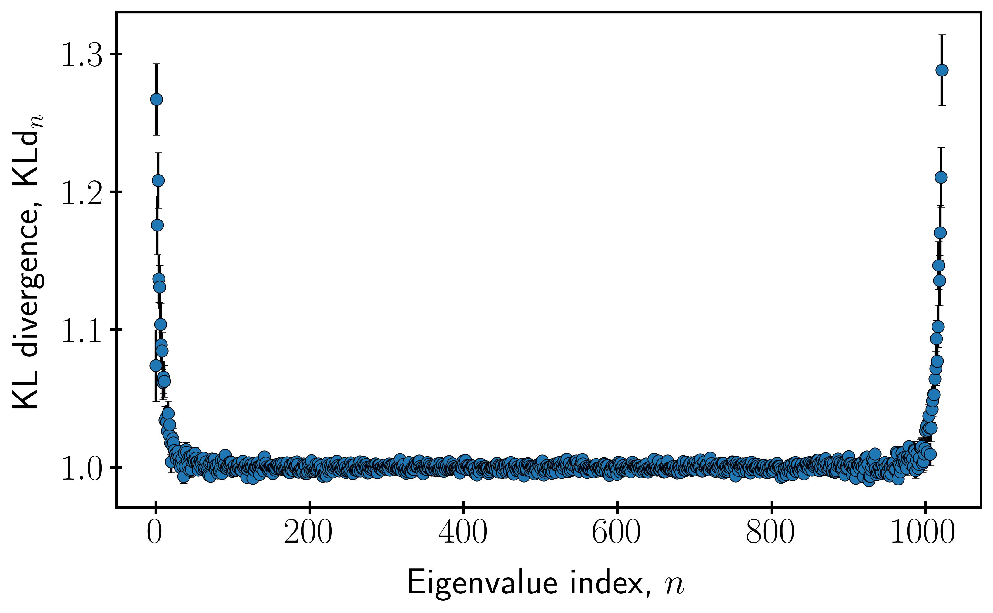
Figure 5: Plot of noise-averaged level spacing ratio (top) and Kullback-Leibler divergence (bottom) of $H_{\rm eff}$ for $L=10$. Error bars represents standard error of mean for $768$ noise realizations.

The results, shown in Figure 5 indicate that the noise-averaged level spacing ratio $\langle r_{n}\rangle$ and KL divergence $\langle\text{KLd}_{n}\rangle$ are consistent with that of Gaussian Unitary Ensemble (GUE): $r_{\rm GUE}=0.599$[27], $\text{KLd}_{\rm GUE}=1$. This confirms that the system will thermalize within the bulk state manifold that is well-described by $H_{\mathrm{eff}}$; note, however, that the data shown actually includes all states, not just the bulk. Furthermore, GUE indicates that thermalization will occur with no conserved quantities besides energy, as is perhaps expected from the unstructured form of $H_{\mathrm{eff}}$. Note, however, that both the level spacing ratio and K-L divergence only probe properties of states that are nearby one another in energy. Therefore, other RMT properties that rely on the complete spectrum and full random matrix form – such as the Wigner semicircle law – are not in general expected to hold. In fact, we will see that the locality structure that exists in $H_{\mathrm{eff}}$ prevents the formation of a Wigner semicircle, as is known to happen in other local ergodic Hamiltonians [29].

III.3 Critical noise strength and its scaling

Having shown that $H_{\mathrm{eff}}$ obeys certain properties of RMT, we now use that to solve for other properties of the noisy algorithm, starting with the critical noise $\delta_{c,\rm gap}$ and its scaling with system size. We start by noting that the algorithm stops giving meaningful answers once the two special states enter into the bulk, i.e., once the gap closes. As evident from Figure 3, this happens near the point where the bulk energies span from $-\pi$ to $\pi$ due to weak dependence of the special state energies on $\delta$. We will study $\delta$-dependence of the special state energies in Section III.4. We define the noise value at this gap-closing point as the critical noise $\delta_{c,\rm gap}$. Since the quasi-energy of the noisy Grover operator is well captured by the effective Hamiltonian up to the point of merger of the special states, we will study the eigenvalues of the later to determine the critical noise and its scaling with system size.

The relevant property of $H_{\mathrm{eff}}$ that determines $\delta_{c,\rm gap}$ is the second moment of its energy distribution. While each realization of $H_{\mathrm{eff}}$ will have nonzero trace (first moment), the fact that $H_{\mathrm{eff}}$ is generated by Paulis implies that this term must be proportional to the identity matrix and therefore creates a uniform energy shift that does not affect the gap-closing transition . To determine the second moment, it is convenient to first shift the spectrum to make $H_{\mathrm{eff}}$ traceless:

$$\tilde{H}_{\rm eff}\equiv H_{\rm eff}-\frac{1}{N}\text{Tr}(H_{\rm eff})\mathbf{1},$$ (27)

which can be done by individually removing the traces from the generators, $\tilde{H}_{j}=H_{j}-\mathrm{Tr}\left(H_{j}\right)/N$. Then the variance is given by

$$E_{0}^{2} \equiv\mathcal{E}\left\{\frac{1}{N}\text{Tr}\left[\tilde{H}_{\text{eff}}^{2}\right]\right\}$$ (28)

$$=\mathcal{E}\left\{\frac{1}{N}\sum_{j,k}\epsilon_{j}\epsilon_{k}\text{Tr}\left[\tilde{H}_{j,\tilde{H}}\tilde{H}_{k,\tilde{H}}\right]\right\}$$ (29)

$$=\frac{1}{3N}\sum_{j}\text{Tr}\left[\tilde{H}_{j}^{2}\right]$$ (30)

$$=\frac{1}{8}(2L^{2}+10L+5),$$ (31)

where we used that $\mathcal{E}\left(\epsilon_{j}\epsilon_{k}\right)=\frac{1}{3}\delta_{jk}$. Notice that $E_{0}\sim L$ comes from the overall gate count, $M\sim L^{2}$; by reducing scaling of the gate count, we would modify this system-size dependence. This scaling is corrobrated numerically in Figure 6.

Having obtained an accurate description of the bulk spectrum, we can derive the scaling of the critical noise $\delta_{c,\rm gap}$. Since the Gaussian distribution does not have a sharp cutoff, let us instead consider when the eigenvalues within, say, $3\sigma$ span the entire Floquet Brillouin zone. Then we can write

$$(-3\delta_{c,\rm gap}E_{0},3\delta_{c,\rm gap}E_{0})=(-\pi,\pi),$$ (32)

which gives

$$3\delta_{c,\rm gap}E_{0}=\pi\implies\delta_{c,\rm gap}=\frac{\pi}{3E_{0}}\implies\delta_{c,\rm gap}\sim L^{-1}.$$

It is easy to see that irrespective of the fraction of eigenvalues we consider that span the entire Brillouin zone, the scaling of the critical noise does not change.

Our analysis gives the correct system-size scaling of $\delta_{c,\rm gap}$, but also shows that a full random matrix treatment is incorrect. Specifically, the drastically different variances of the diagonal and the off-diagonal elements of $H_{\rm eff}$ in Fig.6 deviate from the prediction of a Gaussian Unitary Ensemble (GUE):

$$\mathcal{E}_{\mathrm{GUE}}\left[H^{2}_{nn}\right]=\mathcal{E}_{\mathrm{GUE}}\left[|H_{mn}|^{2}\right]=\frac{\lambda^{2}}{N},$$ (33)

for $1\leq m,n\leq N$, and where $\mathcal{E}_{\mathrm{GUE}}\left[\cdot\right]$ denotes the average over different realizations of the GUE and $\lambda$ sets the units of energy [31]. As a result of this discrepancy in scaling of elements, the distribution of the eigenvalues of $H_{\rm eff}$ deviates from the Wigner’s semicircle law, instead following a normal distribution

$$\rho(E_{\rm eff})=\frac{1}{E_{0}\sqrt{2\pi}}e^{-(E_{\rm eff}/E_{0})^{2}/2}.$$ (34)

Similar deviations from the semicircle law in the energy spectra of many-body systems have been noted in other interacting many-body systems[32, 33, 34], leading to the conclusion that completely random matrices do not accurately represent realistic many body systems. The underlying assumption of these matrices – that each particle interacts simultaneously with all other particles – contradicts the nature of most systems where interactions are predominantly few-body. The presence of $k$-locality here is not immediately obvious due to operator spreading of the $2$-local perturbations when taken in the Heisenberg picture (see Eq. 24). We find strong evidence for approximate $k$-locality from a detailed analysis of matrix elements in $H_{\mathrm{eff}}$, which is done in Appendix A.

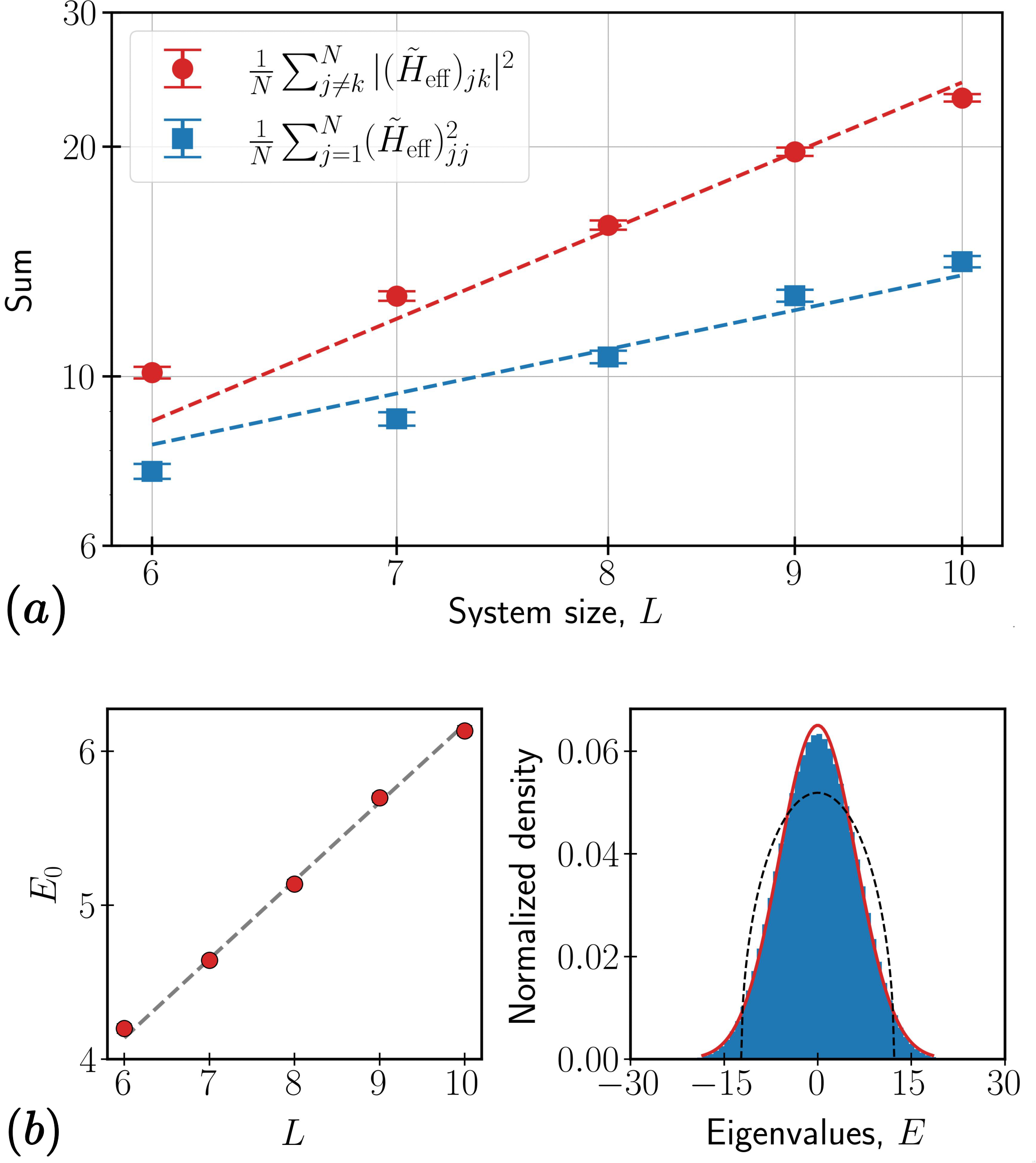
Figure 6: $(a)$ Plot of the sum of squared diagonal and off-diagonal elements of $\tilde{H}_{\rm eff}$ as a function of system size in a log-log plot. Error bars indicate standard error of mean over $512$ noise realizations. The best fit functions $f(x)=aL^{2}$ (off-diagonal) and $g(L)=bL$ (diagonal) are shown with red and blue dashed lines respectively. $(b)$ (Left) $E_{0}$ as a function of system size $L$ calculated using Eq. (28) (red) by averaging over $512$ noise realizations, and is compared with the theoretical prediction given by (31). (Right) Distribution of bulk eigenvalues of $H_{\rm eff}$ for $L=10$, shown along with the normal distribution (Eq. (34)) (red) and Wigner’s semicircle (dashed).

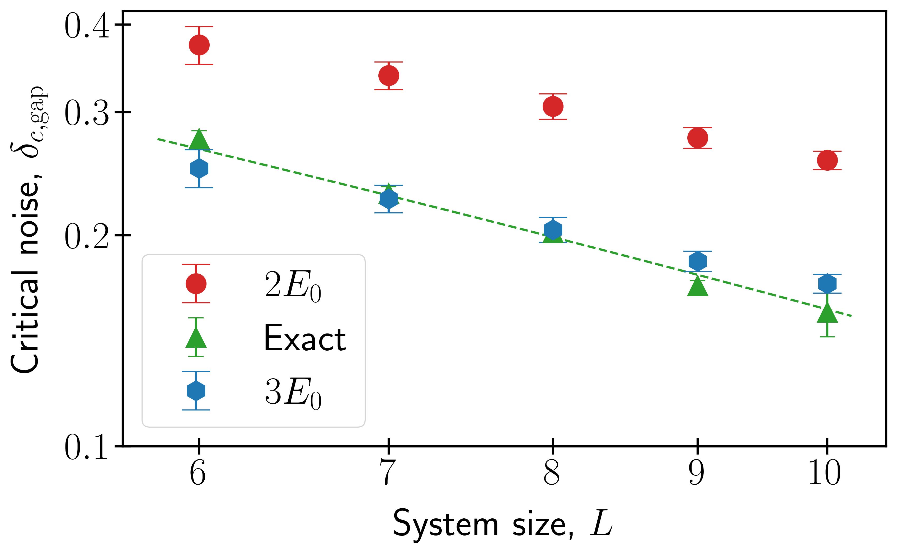
Figure 7: Critical noise strength $\delta_{c,\rm gap}$ as a function of system size shown in a log-log plot. The exact critical noise is calculated at the point where the gap between the two special states and the bulk closes, and are averaged over $20$ noise realizations. The dashed line on the plot represents the best fit line for these exact noises. Predicted critical noises are averaged over $512$ noise realizations and are calculated when the two special states merges into $67\%,(-2E_{0},2E_{0})$, and $99.7\%,(-3E_{0},3E_{0})$ of the bulk eigenvalues spanning the Floquet Brillouin zone.

It is worth noting that the exact value of the gap closing between bulk and special states will not happen precisely at $\delta_{c,\rm gap}$ derived above, but rather a slightly smaller value. This is because the edges of the spectrum of $H_{\mathrm{eff}}$ do not scale identically as its variance. For example, conventional local models have extensive energy range but have energy width scaling as $\sqrt{L}$. However, the energy width $E_{0}\sim L$ is the most important parameter for determining ergodicity, as this is the energy scale on which a finite density of states will come in contact with the special states. The precise scaling of the range of bulk energies, which determines initial gap closing but not ergodicity breaking, will be left for future work.

III.4 Analysis of the special states

Finally, we turn our attention to the two special states. In the absence of noise, the actions of the Grover operator on the states $|0\rangle$ and $|\bar{x}\rangle$ are

$$G_{0}|0\rangle = \left(\frac{2}{N}-1\right)|0\rangle+\frac{2\sqrt{N-1}}{N}|\bar{x}\rangle$$ (35)

$$= -\cos(2\theta)|0\rangle+\sin(2\theta)|\bar{x}\rangle,$$ (36)

$$G_{0}|\bar{x}\rangle = -\frac{2\sqrt{N-1}}{N}|0\rangle+\left(\frac{2}{N}-1\right)|\bar{x}\rangle$$ (37)

$$= -\cos(2\theta)|\bar{x}\rangle-\sin(2\theta)|0\rangle.$$ (38)

Then we can write the noiseless Grover operator in the $\{|0\rangle,|\bar{x}\rangle\}$ block as

$$G^{\rm spec}_{0}=-\begin{bmatrix}\cos(2\theta)&\sin(2\theta)\\ -\sin(2\theta)&\cos(2\theta)\end{bmatrix}=-e^{2i\theta\tau_{y}}.$$ (39)

Now, adding back in the systematic noise, we can repeat our analysis using the effective Hamiltonian within first order perturbation theory and apply it to these special states. Restricting Eq.(25) to the special states manifold by writing it in $|\bar{0}\rangle$ and $|\bar{x}\rangle$ basis,

$$H^{\rm spec}_{\rm eff}\equiv\begin{bmatrix}\langle 0|H_{\rm eff}|0\rangle&\langle 0|H_{\rm eff}|\bar{x}\rangle\\ \langle\bar{x}|H_{\rm eff}|0\rangle&\langle\bar{x}|H_{\rm eff}|\bar{x}\rangle\end{bmatrix},$$ (40)

we obtain:

$$G^{\rm spec}(\delta) \approx -(1-i\delta H^{\rm spec}_{\rm eff})e^{2i\theta\tau_{y}}$$ (41)

$$\approx \exp\{-i(-2\theta\tau_{y}+\delta H^{\rm spec}_{\rm eff}-\pi)\}.$$

The eigenvalues of $-2\theta\tau_{y}+\delta H^{\rm spec}_{\rm eff}-\pi$ capture the quasi-energies of two special states, as shown in Figure 8, once again confirming the effectiveness of first-order perturbation theory.

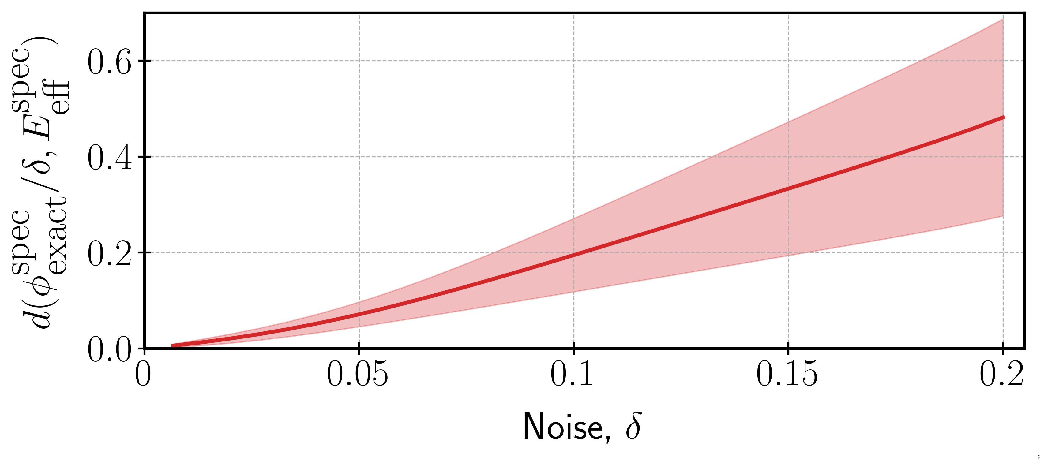
Figure 8: Plot of difference between the exact special states quasi-energy of $G^{\rm spec}(\delta)$ and eigenvalues of $-\theta\tau_{y}+\delta H^{\rm spec}_{\rm eff}$ for $L=8$. Error bands represent the standard error of mean for five noise realizations.

Next, let us analyze the statistical properties of $H^{\rm spec}_{\rm eff}$ to understand the behavior of the two special states in the presence of noise. Taking the logarithm on both sides of Eq. (41):

$$-i\ln G^{\rm spec}\approx\pi\mathbf{1}+2\theta\tau_{y}-\delta H^{\rm spec}_{\rm eff},$$ (42)

we can expand in the Pauli basis to obtain

$$\pi\mathbf{1}+2\theta\tau_{y}-\delta H^{\rm spec}_{\rm eff}=-\delta b_{x}\tau_{x}+(2\theta-\delta b_{y})\tau_{y}-\delta b_{z}\tau_{z}\\ +(\pi-\delta b_{0})\tau_{0}$$

where $b_{j}=\text{tr}(H^{\rm spec}_{\rm eff}\tau_{j})/2$ with $\tau_{x,y,z,0}$ representing the Pauli matrices ($\tau_{0}=\mathbf{1}$). Then the square of the energy gap between the two special states is given by

$$\Delta^{2}\approx 4\left[\delta^{2}b^{2}_{x}+(2\theta-\delta b_{y})^{2}+\delta^{2}b^{2}_{z}\right],$$ (43)

which sets the oscillation frequency between the special states. Averaging over noise configurations and noting that $\mathcal{E}\left[b_{x,y,z,0}\right]=0$, we see that the gap is set by their variance:

$$\mathcal{E}\left[\Delta^{2}\right]\approx 4\left[4\theta^{2}+\delta^{2}\left(\mathcal{E}\left[b^{2}_{x}\right]+\mathcal{E}\left[b^{2}_{y}\right]+\mathcal{E}\left[b^{2}_{z}\right]\right)\right].$$ (44)

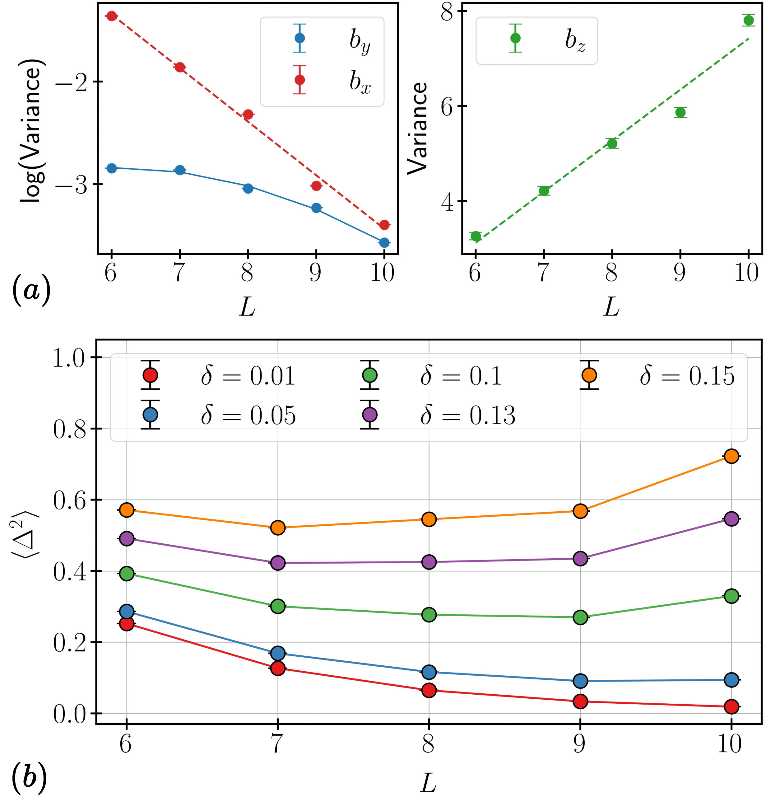
Figure 9: (a) Variance of the coefficients $b_{x},b_{y}$ and $b_{z}$ as a function of system size shown along with their best fit curves. Data is averaged over $512$ noises. (b) Plot of average energy gap squared $\langle\Delta^{2}\rangle$ obtained using Eq. (43) as a function of system size $L$ for different noise strengths. Data is averaged over $512$ noise realizations.

If $H_{\mathrm{eff}}$ were an $N\times N$ GUE random matrix, then $H^{\rm spec}_{\rm eff}$ would be a $2\times 2$ GUE random matrix, for which $\mathcal{E}(b_{x,y,z}^{2})\sim 1/N$. However, as we have seen that non-GUE scaling of the diagonals exists in $H_{\mathrm{eff}}$, we need to more carefully examine whether GUE scaling holds within the special state manifold. As shown in Figure 9, indeed we do not have exponential scaling of these Pauli coefficients nor the gap. While the off-diagonal terms do decrease exponentially fast $\theta^{2},b^{2}_{x},b^{2}_{y}\sim 1/N$, the diagonal term instead increases as $b^{2}_{z}\sim L$. Putting these scalings into Eq. 43, we see that $\mathcal{E}\left[\Delta^{2}\right]\sim A/N+B\delta^{2}/N+CL\delta^{2}$ for some order-1 coefficients $A$, $B$, and $C$. Then, for $\delta\gg\delta_{c,\rm comp}\equiv\sqrt{A/(CLN)}\sim 1/\sqrt{L2^{L}}$, the linear $b_{z}$ term dominates over the $\theta^{2}$ term giving a power-law-large gap. While this increases the oscillation frequency within the special states, it comes at the cost of exponentially decreasing the oscillation amplitude. In the limit of $\delta\gg\delta_{c,\rm comp}$, the states $|0\rangle$ and $|\bar{x}\rangle$ become eigenstates of $G^{\rm spec}(\delta)$ and therefore their probabilities remain at

$$P_{0}(T)=\frac{1}{N},\quad P_{\bar{x}}(T)=1-\frac{1}{N},$$ (45)

at all times $T$, up to exponentially small oscillations. Since there is no longer an order-1 probability of finding the target state at any times, this implies that the model has lost computing power. Therefore, our special state analysis unfortunately implies that at this much smaller critical noise $\delta_{c,\rm comp}\sim L^{-1/2}2^{-L/2}$ we have a “computing transition,” because the algorithm loses computing power for $\delta\apprge\delta_{c,\rm comp}$. By contrast, the gap-closing critical noise $\delta_{c,\rm gap}\sim L^{-1}$ is much larger, but occurs well after computational power has been lost.

Given that the large coefficient $b_{z}$ in $H^{\rm spec}_{\rm eff}$ implies a special basis for the special state manifold, one might hope to recover an exponentially small gap by randomly rotating the basis, e.g., by choosing a different noise model. However, we now argue that this is not possible for any local or $k$-local noise model. The key point is that the relatively larger magnitude of the $b_{z}$ component compared to $b_{x}$ and $b_{y}$ comes from local distinguishability of the states $|0\rangle$ and $|\bar{x}\rangle$, meaning that generic local (or $k$-local) perturbations in $H_{\mathrm{eff}}$ will have a (random) diagonal component in this basis. By contrast, distinguishing the off-diagonal cat states $|0\rangle+e^{i\varphi}|\bar{x}\rangle$ requires global operators. This implies that $\left|\langle 0|H_{\rm eff}|\bar{x}\rangle\right|^{2}\ll\left|\langle 0|H_{\rm eff}|0\rangle\right|^{2},\left|\langle\bar{x}|H_{\rm eff}|\bar{x}\rangle\right|^{2}$, which produces $b_{z}^{2}\gg b_{x,y}^{2}$ for generic $k$-local error models.

IV Conclusion

We analyzed Grover’s algorithm with systematic noise by modeling the Grover operator as a Floquet unitary. We showed that the bulk energy spectrum is well described by an effective Hamiltonian whose spectral statistics match the Gaussian unitary ensemble but whose Gaussian eigenvalue distribution reflects the underlying $k$-local nature of the noise model. We use this structure to derive sharp crossovers between behaviors, finding a gap-closing ergodicity transition at relatively large noise strength $\delta_{c,\rm gap}\sim 1/L$ and a separate transition where computational power is lost above an exponentially small noise strength $\delta_{c,\rm comp}\sim L^{-1/2}2^{-L/2}$. The random matrix theory model enables analytical predictions for many quantities, such as these noise thresholds and dynamics of the initial state.

The machinery we have developed for this simplest case of Grover’s algorithm with a single solution should provide insight into more generally applying many-body physics approaches to noisy quantum algorithms. For example, we can readily see that Grover’s algorithm with multiple solutions exhibits the same phenomenology, since the core aspects of a degenerate gapped bulk and cat-like special eigenstates holds there as well. A more interesting variant is to instead consider decompositions of the multiqubit Toffoli gate using ancilla qubits. If the ancillas are erased before reuse, they will behave similar to a conventional noise channel which previous results suggest will yield and exponentially small error threshold. On the other hand, if the ancillas are uncomputed and the measured and postselected, the resulting dynamics is noisy but non-unitary, similar to dynamics generated by non-Hermitian Hamiltonians. Non-Hermitian dynamics are known to have qualitatively different phase structures than their Hermitian counterparts. How this affects the phase structure and noise tolerance of Grover’s algorithm remains a fascinating open question.

Another important avenue to investigate for Grover’s algorithm is the role of non-$k$-local gating. While most controllable quantum computers rely on $k$-local gates - even if swap operations or atomic repositioning relax the assumption of strict spatial locality – there are potential routes to remove this restriction by using a non-local cavity mode or the long-range tails of Rydberg blockade [35]. This not only allows more efficient decomposition of the multicontrolled gates, but also implies that systematic gate errors will be nonlocal as well. Nonlocal errors in $H_{\mathrm{eff}}$ will cause it to behave more like a proper GUE random matrix, for which a power law noise tolerance $\delta\sim 1/L^{\alpha}$ can in principle be admitted for both the ergodicity transition and the computational phase transition. In the NISQ era of finite noise, it is crucial to know these noise scalings in order to determine near-term experimental feasibility. We therefore suggest that non-local gating may be a pathway to drastically improved noise-tolerance for Grover’s algorithm, based on our analytical understanding through random matrix theory.

Finally, while Grover’s algorithm provides a concrete example of Floquet analysis in the context of useful quantum algorithms, the eventual goal is to apply similar tools to a wider class of algorithms. Rather than approaching such problem on an individual basis, we would hope to find inspiration for doing so in “grand unified” theories of quantum computation [36]. While no Floquet structure is immediately apparently in such prescriptions, we might hope to find a constituent block on which similar analysis can be applied and use that insight to understand systematic noise tolerance of a wider class of quantum algorithms.

V Acknowledgements

We thank Sarang Gopalakrishnan, Arjun Mirani, and Junpeng Hou for useful discussions. This work was performed with support from the National Science Foundation (NSF) through award numbers OMR-2228725 and DMR-1945529, the Welch Foundation through award number AT-2036-20200401, and DARPA through award number HR00112330022 (M.K. and S.D.). V.K. acknowledges support from the Office of Naval Research Young Investigator Program (ONR YIP) under Award Number N00014-24-1-2098, the Alfred P. Sloan Foundation through a Sloan Research Fellowship and the Packard Foundation through a Packard Fellowship in Science and Engineering. C.Z. acknowledges support from AFOSR (FA9550-20-1-0220), NSF (PHY-2409943, OMR-2228725, ECCS-2411394, OSI-2326628). Part of this work was performed at the Aspen Center for Physics, which is supported by NSF grant No. PHY-1607611, and at the Kavli Institute for Theoretical Physics, which is supported by NSF grant No. PHY-1748958.

Appendix A Structure of effective Hamiltonian

As shown in the main text, the effective noise Hamiltonian $H_{\mathrm{eff}}$ does not show full random matrix statistics. Here we analyze the structure further.

We start with a heatmap of the magnitude of the elements of $H_{\rm eff}$ in the computational ($z$) basis and in the eigenbasis of $G_{0}$ in Figure 10 . A random matrix would show uniform average color in any basis, with no clear distinction between diagonal and off-diagonal matrix elements. By contrast, $H_{\mathrm{eff}}$ shows band like structures with strongest matrix elements corresponding to the diagonal. This follows from the $k$-locality of the gate perturbations in the structure of $H_{\rm eff}$ (Eq. (24)), which means that only a limited number of spins can be flipped in the $z$-basis (and the same applies to the eigenbasis of $G_{0}$).

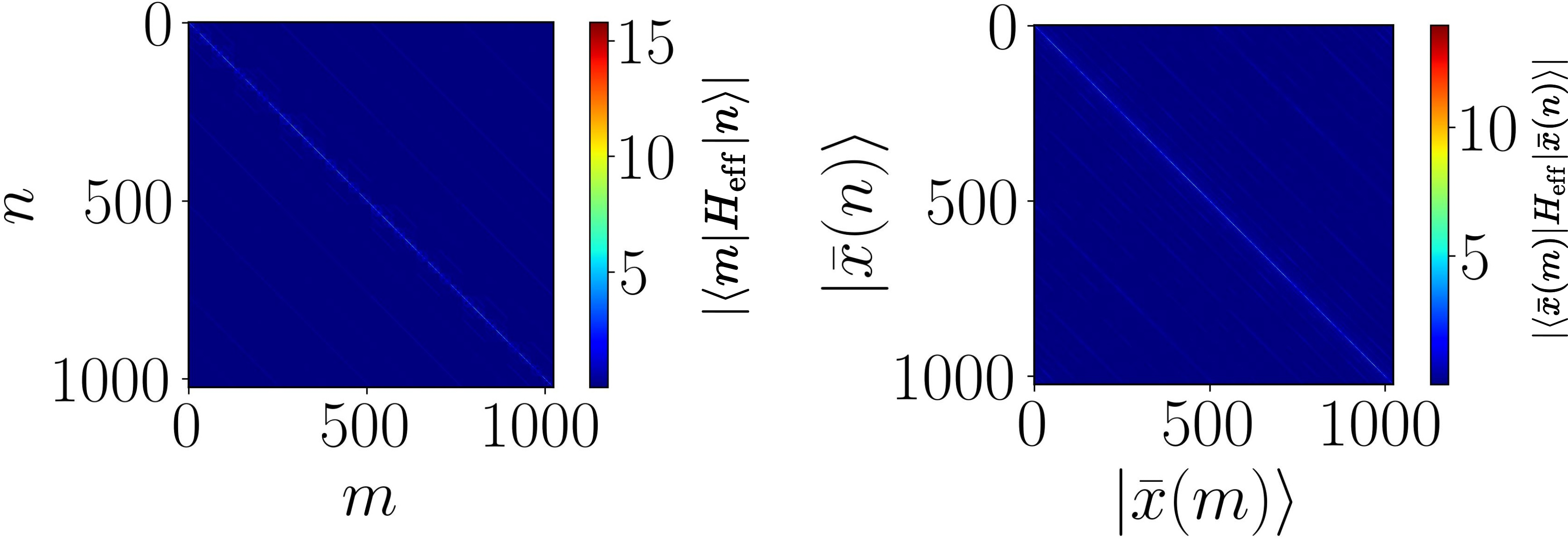
Figure 10: Heatmaps of the magnitude of the elements of $H_{\rm eff}$ in the computational basis $\{|k\rangle\}$ (left) and in the eigenbasis of $G_{0}$, $\{|\bar{x}(k)\rangle\}$(right) for $L=10$. The colorbar represents the absolute value of the elements in both the bases.

Appendix B Dynamics of the special states

In addition to gap-closing and computational phase transitions, the random matrix treatment gives analytical predictions for nearly all properties of the algorithm’s behavior. In this section, we describe the behavior of special state dynamics, which is the most relevant dynamical feature that allows the unperturbed algorithm $G_{0}$ to be successful. While we can make predictions for how systematic noise modifies these dynamics, their computational relevance is limited to the very small regime of $\delta\ll\delta_{c,\rm comp}$. However, we can also make concrete predictions for ergodicity breaking as long as $\delta<\delta_{c,\rm gap}$.

Before directly examining dynamics, it is worth briefly thinking about the behavior of perturbation theory in this degenerate many-body setting. In particular, given that we start within the special state manifold, does a finite probability of staying in this manifold survive at late time?

In order to address this question, we define the effective Hamiltonian within the special state manifold as

$$H^{{}^{\prime}}(\delta) = 2\theta\tau_{y}-\delta H^{\rm spec}_{\rm eff}$$

$$= -\Delta(\cos\theta^{{}^{\prime}}\tau_{z}+\sin\theta^{{}^{\prime}}(\tau_{x}\cos\phi+\tau_{y}\sin\phi))$$

where $\theta^{{}^{\prime}}\equiv\theta^{{}^{\prime}}(\delta)$. Then we write the eigenstates of $H^{{}^{\prime}}(\delta)$ as

$$|\psi^{(0)}_{1}\rangle = \cos\left(\frac{\theta^{{}^{\prime}}}{2}\right)|0\rangle+e^{i\phi}\sin\left(\frac{\theta^{{}^{\prime}}}{2}\right)|\bar{x}\rangle,$$ (46)

$$|\psi^{(0)}_{2}\rangle = \sin\left(\frac{\theta^{{}^{\prime}}}{2}\right)|0\rangle-e^{i\phi}\cos\left(\frac{\theta^{{}^{\prime}}}{2}\right)|\bar{x}\rangle,$$ (47)

with energies $\epsilon^{(0)}_{1,2}$ near $\pi$. Then we can write,

$$G(\delta) = e^{-iH_{\rm eff}}G_{0}\approx e^{-i\delta H^{{}^{\prime}}_{\rm eff}}e^{-i\delta H^{\rm spec}_{\rm eff}}G_{0}=e^{-i\delta H^{{}^{\prime}}_{\rm eff}}\tilde{G},$$

where $H_{\rm eff}$ is divided into $H^{\rm spec}_{\rm eff}$, a block containing the two special states, and the remainder $H^{{}^{\prime}}_{\rm eff}=H_{\rm eff}-H^{\rm spec}_{\rm eff}$ such that $\tilde{G}|\psi^{(0)}_{j}\rangle=e^{-i\epsilon^{(0)}_{j}}|\psi^{(0)}_{j}\rangle$. Next, consider the action of $G(\delta)$ on the special states,

$$G(\delta)|\psi_{j}\rangle=e^{-i\delta H^{\rm spec}_{\rm eff}}\tilde{G}|\psi_{j}\rangle,$$ (48)

expanding both sides up to the first order in $\delta$, we get

$$e^{-i\delta H^{{}^{\prime}}_{\rm eff}} \tilde{G} (|\psi^{(0)}_{j}\rangle+\delta|\psi^{(1)}_{j}\rangle+\cdots)$$

$$= e^{-i(E^{(0)}_{j}+\delta E^{(1)}_{j}+\cdots)}(|\psi^{(0)}_{j}\rangle+\delta|\psi^{(1)}_{j}\rangle+\cdots).$$

Taking the matrix element with bulk state $|\bar{x}_{k}\rangle$ and keeping terms up to order $\delta$, we get

$$\langle\bar{x}_{k}|\psi^{(1)}_{j}\rangle(1-e^{-iE^{(0)}_{j}}) = ie^{-iE^{(0)}_{j}}\langle\bar{x}_{k}|H^{{}^{\prime}}_{\rm eff}|\psi^{(0)}_{j}\rangle,$$ (49)

where we have used $\langle\bar{x}_{k}|\tilde{G}|\psi^{(0)}_{j}\rangle=\langle\bar{x}_{k}|\psi^{(0)}_{j}\rangle=0$. Next using $E^{(0)}_{j}\approx\pi$, we obtain

$$\langle\bar{x}_{k}|\psi^{(1)}_{j}\rangle = \frac{-i}{2}\langle\bar{x}_{k}|H^{{}^{\prime}}_{\rm eff}|\psi^{(0)}_{j}\rangle.$$ (50)

Therefore, the net bulk occupation in the dressed eigenstate $|\psi_{j}\rangle$ is approximately

$$P_{\text{bulk},j} = \sum_{k}|\delta\langle\bar{x}_{k}|\psi^{(1)}_{j}\rangle|^{2}$$ (51)

$$= \frac{\delta^{2}}{4}\sum_{k}|\langle\bar{x}_{k}|H^{{}^{\prime}}_{\rm eff}|\psi^{(0)}_{j}\rangle|^{2}.$$

While the exact expression for this off-diagonal matrix element, $|\langle\bar{x}_{k}|H^{{}^{\prime}}_{\rm eff}|\psi^{(0)}_{j}\rangle|^{2}$, depends on the particular choice of $k$, the sum over these matrix elements is constrained to be no larger than $E_{0}^{2}$ (at least upon averaging over $j$) due to the fact that $\mathrm{Tr}[H_{\mathrm{eff}}^{2}]=E_{0}^{2}N$ can be broken up into diagonal and off-diagonal pieces and the diagonals already given the $E_{0}^{2}N$ scaling. Therefore, the off-diagonal sum must give $E_{0}^{2}N$ or smaller, and the lack of summing over $j$ in Eq. 51 removes the multiplicative factor $N$. Assuming that the sum saturates this scaling, we conclude that

$$P_{\text{bulk},j}\approx\frac{\delta^{2}E_{0}^{2}}{4}\sim\left(\delta/\delta_{c,\rm gap}\right)^{2}.$$ (52)

Therefore, the bulk occupation remains finite below $\delta_{c,\rm gap}$, meaning that the special states will also remain finitely occupied at late times and thus break ergodicity as we have claimed.

Next, let us analyze the behavior of the probabilities $P_{0}(t)$ and $P_{\bar{x}}(t)$ in presence of noise. Consider the following ansatz for the two special states within first order in noise:

$$|\psi_{1}\rangle = \left(1-P_{b}\right)^{1/4}\left[\cos\left(\frac{\theta^{\prime}}{2}\right)|\bar{x}\rangle+e^{i\phi^{\prime}}\sin\left(\frac{\theta^{\prime}}{2}\right)|0\rangle\right]$$

$$+\delta\sum_{k}|\bar{x}_{k}\rangle\langle\bar{x}_{k}|\psi_{1}^{(1)}\rangle,$$

$$|\psi_{2}\rangle = \left(1-P_{b}\right)^{1/4}\left[\sin\left(\frac{\theta^{\prime}}{2}\right)|\bar{x}\rangle-e^{i\phi^{\prime}}\cos\left(\frac{\theta^{\prime}}{2}\right)|0\rangle\right]$$

$$+\delta\sum_{k}|\bar{x}_{k}\rangle\langle\bar{x}_{k}|\psi_{2}^{(1)}\rangle,$$

where we will see that $P_{b}$ is a related parameter that describes late time occupation of the bulk given our actual starting state. This is an unusual ansatz, as it dresses the zeroth order result from degenerate perturbation theory by a non-perturbative overall rescaling of the amplitude, $\left(1-P_{b}\right)^{1/4}$. This comes from the finite “leakage” into the bulk at late times but, as we’ll show, seems to give a self-consistent picture of the full dynamics.

With this ansatz, we can write the initial state of the system as

$$|\psi(0)\rangle = |x\rangle\approx|\bar{x}\rangle$$ (53)

$$= \left(1-P_{b}\right)^{1/4}\left[\cos\left(\frac{\theta^{\prime}}{2}\right)|\psi_{1}\rangle+\sin\left(\frac{\theta^{\prime}}{2}\right)|\psi_{2}\rangle\right]$$

$$+\sum_{k}c_{k}|\psi_{k}\rangle,$$

where $k$ labels the $N-2$ bulk energy eigenstates. But $|\bar{x}\rangle$ is normalized, so

$$1=\sqrt{1-P_{b}}+\sum_{k}\left|c_{k}\right|^{2}\implies|c_{k}|^{2}\sim\frac{1-\sqrt{1-P_{b}}}{N}.$$ (54)

Having decomposed the initial state into eigenstates (Eq. 53), we can now easily calculate its time evolution as

$$|\psi(t)\rangle = \left(1-P_{b}\right)^{1/4}[\cos\left(\frac{\theta^{\prime}}{2}\right)e^{-iE_{1}t}|\psi_{1}\rangle$$

$$+\sin\left(\frac{\theta^{\prime}}{2}\right)e^{-iE_{2}t}|\psi_{2}\rangle]+\sum_{k}c_{k}e^{-iE_{k}t}|\psi_{k}\rangle$$

$$\equiv\sum_{j}c_{j}e^{-iE_{j}t}|\psi_{j}\rangle,$$

where $t$ is the number of time steps. Then we simply need to calculate observables.

One important observable is the probability to find ourselves in $|\bar{x}\rangle$, which is approximately the Loschmidt echo:

$$P_{\bar{x}}(t) =\left|\langle\bar{x}|\psi(t)\rangle\right|^{2}\approx\left|\langle\psi(0)|\psi(t)\rangle\right|^{2}$$

$$=\sum_{jj^{\prime}}\left|c_{j}\right|^{2}\left|c_{j^{\prime}}\right|^{2}e^{-i(E_{j}-E_{j^{\prime}})t}$$

$$=\underbrace{P_{\bar{x}}(\text{average as }t\to\infty)}_{\text{A}:~{}j=j^{\prime}}+$$

$$\;\;\;\underbrace{2\sin^{2}\left(\theta^{\prime}\right)\cos^{2}\left(\theta^{\prime}\right)\left(1-P_{b}\right)\cos\left[\left(E_{1}-E_{2}\right)t\right]}_{\text{B: Usual Grover oscillations},~{}j=1,~{}j^{\prime}=2}+$$

$$\;\;\;\underbrace{\sum_{k}\left|c_{1}\right|^{2}\left|c_{k}\right|^{2}e^{-i(E_{1}-E_{k})t}+c.c.+\left(1\to 2\right)}_{\text{C: Damped oscillations due to bulk},~{}j=1,~{}j^{\prime}=k}+$$

$$\;\;\;\underbrace{\sum_{k\neq k^{\prime}}\left|c_{k}\right|^{2}\left|c_{k^{\prime}}\right|^{2}e^{-i(E_{k}-E_{k^{\prime}})t}}_{\text{D: Direct bulk decay},~{}j=k\neq j^{\prime}=k^{\prime}}.$$ (55)

Let us analyze Eq.(55) term by term.

Term A: Late-time average: The existence of a non-exponentially-small occupation in state $|\bar{x}\rangle$ is a clear indication of nonergodicity. It will differ between noise realizations, but we can estimate its noise average (which is equal to participation ratio in the eigenstate basis):

$$\overline{P_{\bar{x}}} =\left(1-P_{b}\right)\left[\cos^{4}\left(\frac{\theta^{\prime}}{2}\right)+\sin^{4}\left(\frac{\theta^{\prime}}{2}\right)\right]+\sum_{k}\underbrace{\left|c_{k}\right|^{4}}_{\sim\left(P_{b}/N\right)^{2}}$$

$$\approx\left(1-P_{b}\right)\left[\cos^{4}\left(\frac{\theta^{\prime}}{2}\right)+\sin^{4}\left(\frac{\theta^{\prime}}{2}\right)\right]+O(1/N)$$

Before continuing, it’s worth doing a similar calculation for the target state:

$$\overline{P_{0}} = \left(\sqrt{1-P_{b}}\right)[\cos^{2}\left(\frac{\theta^{\prime}}{2}\right)\left|\langle 0|\psi_{1}\rangle\right|^{2}$$

$$+\sin^{2}\left(\frac{\theta^{\prime}}{2}\right)\left|\langle 0|\psi_{2}\rangle\right|^{2}]+\underbrace{\sum_{k}\left|c_{k}\right|^{2}\left|\langle 0|\psi_{k}\rangle\right|^{2}}_{O(1/N)}$$

$$\approx\left(1-P_{b}\right)\left[2\cos^{2}\left(\frac{\theta^{\prime}}{2}\right)\sin^{2}\left(\frac{\theta^{\prime}}{2}\right)\right]$$

$$\implies\overline{P_{\bar{x}}}+\overline{P_{0}} =1-P_{b}$$

as expected – $P_{b}$ is the late-time probability to leave the special state manifold.

Term B: Grover oscillations: These are the oscillations that occur at frequency $\Delta\sim 1/\sqrt{N}$ in the absence of noise and with notable modifications in both amplitude and frequency in the range $\delta_{c,\rm comp}<\delta<\delta_{c,\rm gap}$. Specifically, it is clear that, when $P_{b}>0$ and/or $\theta^{\prime}\neq\pi/2$ (as happens for finite $\delta$), oscillation amplitude is less than unity.

Term C: Damped oscillations from bulk continuum: Due to the $\pi$ gap between bulk and special states, there are fast (period 2) oscillations in the occupation. However, since the bulk has finite spectral width, these oscillations are damped. The gap $\Delta$ between $E_{1}$ and $E_{2}$ will not be resolvable on the decay time-scale, so for all intents and purposes we can just set both of these to $\pi$. Using the Gaussian density of states obtained in the main text,

$$\nu(E)=\frac{N}{\sqrt{2\pi\delta^{2}E_{0}^{2}}}e^{-E^{2}/(2\delta^{2}E_{0}^{2})},$$ (56)

we get,

$$P_{\bar{x}}^{\text{C}}(t)=2\left(-1\right)^{t}\left(\sqrt{1-P_{b}}-1+P_{b}\right)e^{-\delta^{2}E_{0}^{2}t^{2}/2},$$ (57)

which is simply Gaussian relaxation on time scale $\tau\sim 1/\left(\delta E_{0}\right)\sim\delta_{c,\rm gap}/\delta$ that we expect to see. Notice that this is a fast $O(1)$ time scale as long we keep $\delta/\delta_{c,\rm gap}$ fixed as we take $L$ large.

Term D: Bulk decay: Finally, the last term tells us how Loschmidt echo of a given state – in this case $|\bar{x}\rangle$ – decays when propagated by the random bulk matrix $H_{\rm eff}$. Again, using the Gaussian approximation for density of states, we find

$$P_{\bar{x}}^{D}(t) \approx \frac{\left(1-\sqrt{1-P_{b}}\right)^{2}}{N^{2}}$$

$$\times\int dEdE^{\prime}\nu(E)\nu(E^{\prime})\cos\left(\left(E-E^{\prime}\right)t\right),$$

$$= \left(1-\sqrt{1-P_{b}}\right)^{2}e^{-\delta^{2}E_{0}^{2}t^{2}}.$$

This is similar to the decay rate of the $2T$-periodic oscillations (term C) with a rate that is $\sqrt{2}$ times faster. Lastly, as a sanity check, let us confirm that $P_{\bar{x}}(0)=1$:

$$P_{\bar{x}}^{A}(0)+p_{\bar{x}}^{B}(0) = \left(1-P_{b}\right)\left[\cos^{4}\left(\frac{\theta^{\prime}}{2}\right)+\sin^{4}\left(\frac{\theta^{\prime}}{2}\right)\right],$$

$$+2\sin^{2}\left(\theta^{\prime}\right)\cos^{2}\left(\theta^{\prime}\right)\left(1-P_{b}\right),$$

$$= 1-P_{b}.$$

$$P_{\bar{x}}^{C}(0)+P_{\bar{x}}^{D}(0) = 2\left(\sqrt{1-P_{b}}-1+P_{b}\right)+\left(1-\sqrt{1-P_{b}}\right)^{2},$$

$$= P_{b}.$$

Thus

$$P_{\bar{x}}(0)=1.$$ (58)

The predicted behaviors above are seen in Figure 11. Note that the period-$2$ oscillations do appear on close inspection of the short-time behavior (cf. the sharp jump in the curve for $\delta=0.17$ in orange), but are not clear on the longer time scale plotted here.

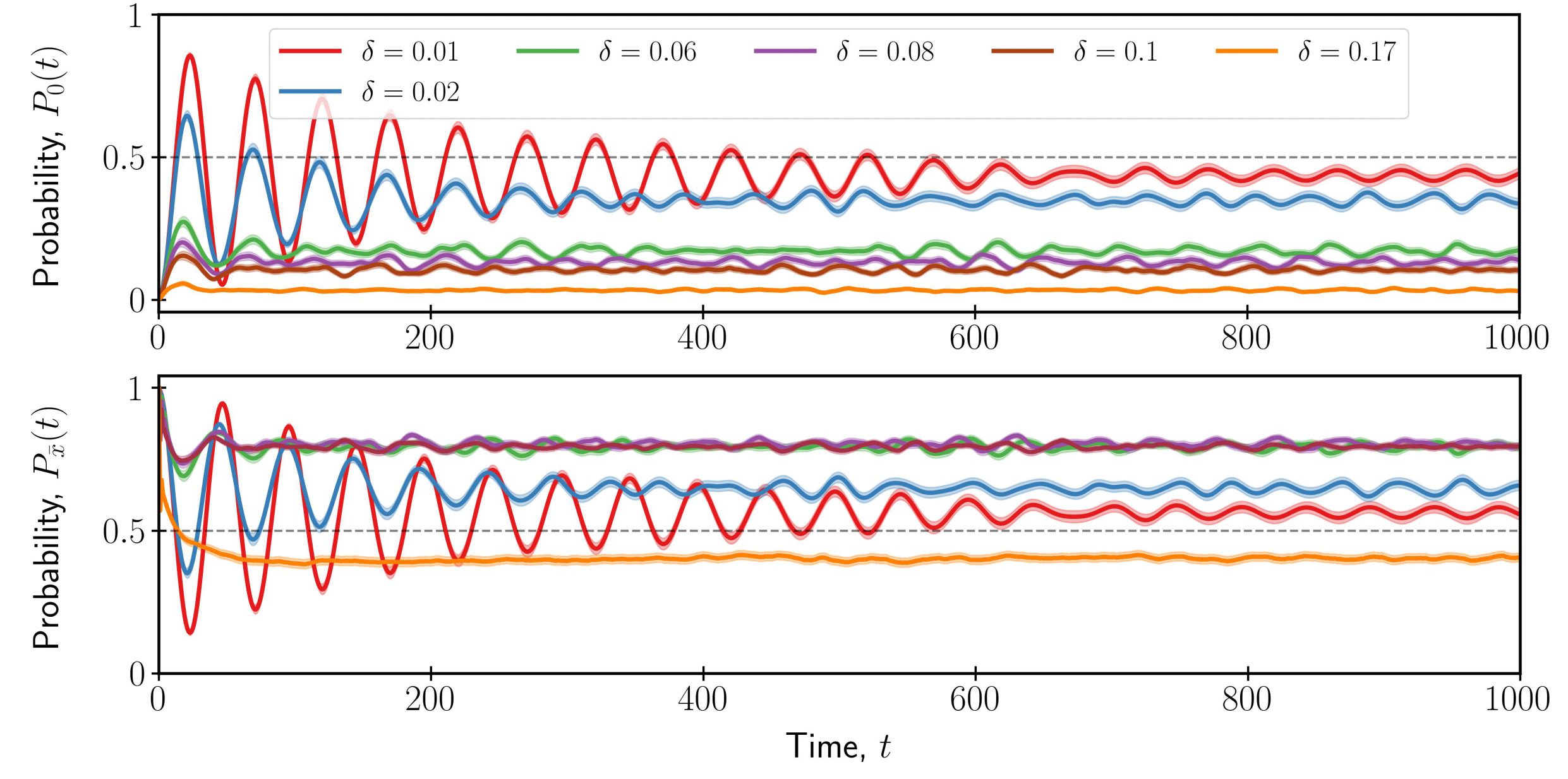
Figure 11: Plot of average probability $P_{0}(t)$ and $P_{\bar{x}}(t)$ for $L=10$ as a function of time steps for different noise strengths: $0.01<\delta_{c,\rm comp}\approx 0.02<0.06<0.08<0.1<\delta_{c,\rm gap}\approx 0.15<0.17$. When $\delta<\delta_{c,\rm gap}$, the probabilities oscillates with a larger frequency but smaller amplitude as compared to the noiseless case. The noises $\delta=0.06,0.08,0.1$ lie in between $\delta_{c,\rm gap}$ and $\delta_{c,\rm comp}$, for which there is no significant change in the probabilities as anticipated from the above analytical calculation. Noise $\delta=0.17>\delta_{c,\rm comp}$ represents the noise dominated dynamics. Error bands represents the standard error of mean for $256$ noise realizations.

References

- Preskill [2018] J. Preskill, Quantum Computing in the NISQ era and beyond, Quantum 2, 79 (2018).
- Fauseweh [2024] B. Fauseweh, Quantum many-body simulations on digital quantum computers: State-of-the-art and future challenges, Nature Communications 15, 2123 (2024).
- Bharti et al. [2022] K. Bharti, A. Cervera-Lierta, T. H. Kyaw, T. Haug, S. Alperin-Lea, A. Anand, M. Degroote, H. Heimonen, J. S. Kottmann, T. Menke, W.-K. Mok, S. Sim, L.-C. Kwek, and A. Aspuru-Guzik, Noisy intermediate-scale quantum algorithms, Rev. Mod. Phys. 94, 015004 (2022).
- Grover [1996] L. K. Grover, A fast quantum mechanical algorithm for database search, in Symposium on the Theory of Computing (1996).
- Figgatt et al. [2017] C. Figgatt, D. L. Maslov, K. A. Landsman, N. M. Linke, S. Debnath, and C. R. Monroe, Complete 3-qubit grover search on a programmable quantum computer, Nature Communications 8 (2017).
- Zhang et al. [2021] K. Zhang, P. Rao, K. Yu, H. Lim, and V. E. Korepin, Implementation of efficient quantum search algorithms on nisq computers, Quantum Information Processing 20 (2021).
- Zhang et al. [2022] K. Zhang, K. Yu, and V. E. Korepin, Quantum search on noisy intermediate-scale quantum devices, Europhysics Letters 140 (2022).
- Long et al. [2000] G. L. Long, Y. S. Li, W. L. Zhang, and C. C. Tu, Dominant gate imperfection in grover’s quantum search algorithm, Phys. Rev. A 61, 042305 (2000).
- Shenvi et al. [2003] N. Shenvi, K. R. Brown, and K. B. Whaley, Effects of a random noisy oracle on search algorithm complexity, Phys. Rev. A 68, 052313 (2003).
- Salas [2008] P. J. Salas, Noise effect on grover algorithm, The European Physical Journal D 46, 365 (2008).
- Pablo-Norman and Ruiz-Altaba [1999] B. Pablo-Norman and M. Ruiz-Altaba, Noise in grover’s quantum search algorithm, Phys. Rev. A 61, 012301 (1999).
- Shapira et al. [2003] D. Shapira, S. Mozes, and O. Biham, Effect of unitary noise on grover’s quantum search algorithm, Phys. Rev. A 67, 042301 (2003).
- Boyer et al. [1998] M. Boyer, G. Brassard, P. Høyer, and A. Tapp, Tight bounds on quantum searching, Fortschritte der Physik 46, 493 (1998).
- Zalka [1999] C. Zalka, Grover’s quantum searching algorithm is optimal, Phys. Rev. A 60, 2746 (1999).
- Oka and Kitamura [2019] T. Oka and S. Kitamura, Floquet engineering of quantum materials, Annual Review of Condensed Matter Physics 10, 387 (2019).
- Bukov et al. [2015] M. Bukov, L. D’Alessio, and A. Polkovnikov, Universal high-frequency behavior of periodically driven systems: from dynamical stabilization to floquet engineering, Advances in Physics 64, 139 (2015).
- [17] G. Floquet, Sur les équations différentielles linéaires à coefficients périodiques, Annales Scientifiques De L Ecole Normale Superieure 12, 47.
- Nielsen and Chuang [2010] M. A. Nielsen and I. L. Chuang, Quantum Computation and Quantum Information: 10th Anniversary Edition (Cambridge University Press, 2010).
- Barenco et al. [1995] A. Barenco, C. H. Bennett, R. Cleve, D. P. DiVincenzo, N. Margolus, P. Shor, T. Sleator, J. A. Smolin, and H. Weinfurter, Elementary gates for quantum computation, Phys. Rev. A 52, 3457 (1995).
- Saeedi and Pedram [2013] M. Saeedi and M. Pedram, Linear-depth quantum circuits for -qubit toffoli gates with no ancilla, Phys. Rev. A 87, 062318 (2013).
- Note [1] The decomposition shown requires gate range proportional to , but the authors argue that finite-range gates still allow depth .
- Page [1993] D. N. Page, Average entropy of a subsystem, Phys. Rev. Lett. 71, 1291 (1993).
- Note [2] Here, the origin of time in the Heisenberg picture is defined as the end of the Floquet cycle, such that Heisenberg evolution “rewinds” the action of .
- Oganesyan and Huse [2007] V. Oganesyan and D. A. Huse, Localization of interacting fermions at high temperature, Phys. Rev. B 75, 155111 (2007).
- Kullback and Leibler [1951] S. Kullback and R. A. Leibler, On Information and Sufficiency, The Annals of Mathematical Statistics 22, 79 (1951).
- Luitz et al. [2015] D. J. Luitz, N. Laflorencie, and F. Alet, Many-body localization edge in the random-field heisenberg chain, Phys. Rev. B 91, 081103 (2015).
- Atas et al. [2013] Y. Y. Atas, E. Bogomolny, O. Giraud, and G. Roux, Distribution of the ratio of consecutive level spacings in random matrix ensembles, Phys. Rev. Lett. 110, 084101 (2013).
- Note [3] We calculated the KL divergence of the standard Gaussian Unitary Ensemble (GUE) by generating GUE matrices of size using the package TeNPy.
- Rodriguez-Nieva et al. [2023] J. F. Rodriguez-Nieva, C. Jonay, and V. Khemani, Quantifying quantum chaos through microcanonical distributions of entanglement, arXiv preprint arXiv:2305.11940 (2023).
- Note [4] The trace is explicitly given by , whose noise-averaged value is equal to zero, while its standard deviation is extensive: given gates.
- Haake [2010] F. Haake, Quantum Signatures of Chaos (Springer Berlin, 2010).
- Bohigas and Flores [1971] O. Bohigas and J. Flores, Two-body random hamiltonian and level density, Physics Letters B 34, 261 (1971).
- French and Wong [1970] J. French and S. Wong, Validity of random matrix theories for many-particle systems, Physics Letters B 33, 449 (1970).
- Torres-Herrera et al. [2016] E. J. Torres-Herrera, J. Karp, M. Távora, and L. F. Santos, Realistic many-body quantum systems vs. full random matrices: Static and dynamical properties, Entropy 18, 10.3390/e18100359 (2016).
- Anikeeva et al. [2021] G. Anikeeva, O. Marković, V. Borish, J. A. Hines, S. V. Rajagopal, E. S. Cooper, A. Periwal, A. Safavi-Naeini, E. J. Davis, and M. Schleier-Smith, Number partitioning with grover’s algorithm in central spin systems, PRX Quantum 2, 020319 (2021).
- Martyn et al. [2021] J. M. Martyn, Z. M. Rossi, A. K. Tan, and I. L. Chuang, Grand unification of quantum algorithms, PRX Quantum 2, 040203 (2021).