Fundamental constants from photon-photon scattering in three-beam collisions
Abstract
Direct measurement of the elastic scattering of real photons on an electromagnetic field would allow the fundamental low-energy constants of quantum electrodynamics (QED) to be experimentally determined. We show that scenarios involving the collision of three laser beams have several advantages over conventional two-beam scenarios. The kinematics of a three-beam collision allows for a higher signal-to-noise ratio in the detection region, without the need for polarimetry and separates out contributions from different orders of photon scattering. A planar configuration of colliding a photon beam from an x-ray free electron laser with two optical beams is studied in detail. We show that measurements of elastic photon scattering and vacuum birefringence are possible with currently available technology.
I Introduction
Quantum electrodynamics (QED) predicts that the coupling between strong electromagnetic fields mediated by virtual particle/anti-particle pairs imbues the vacuum with nonlinear properties. This breaks the superposition principle of classical electrodynamics, allowing for the self interaction of electromagnetic fields. Microscopically, this self interaction corresponds to photon-photon scattering. Despite being predicted almost a century ago Sauter (1931); Halpern (1933); Heisenberg (1934); Heisenberg and Euler (1936); Schwinger (1951); Toll (1952) a direct measurement of on-shell photon-photon scattering and the predicted birefringence of the quantum vacuum have yet to be made, although Delbrück scattering Delbrück (1933); Schumacher et al. (1975) (the scattering of photons in a Coulomb field of a nucleus, i.e. involving off-shell photons) and more recently scattering of quasi-real photons in ultra-peripheral collisions of heavy ions in the ATLAS Aaboud et al. (2017); Aad et al. (2019) and CMS Sirunyan et al. (2019) experiments have been observed. It has also been reported Brandenburg et al. (2023) that the STAR Adam et al. (2021) experiment measured an indirect signal of vacuum birefringence in the spectrum of electron-positron pairs created in ultra-peripheral heavy-ion collisions. The lack of verification of photon-photon scattering with real photons can be attributed to two obstacles: the small size of the photon-photon scattering cross section and the high background generated when colliding beams of photons. As laser technology continues to improve and provide photon sources with an ever-higher flux, experimental verification of real photon-photon scattering seems achievable. There have been numerous suggestions for how to increase the signal-to-noise ratio in discovery experiments employing intense laser pulses, such as ‘vacuum diffracting’ a probe beam with an intense pump beam Di Piazza et al. (2006); King et al. (2010a, b); Kryuchkyan and Hatsagortsyan (2011); Tommasini and Michinel (2010); Monden and Kodama (2011); King and Keitel (2012); Jin et al. (2022), ‘vacuum reflection’ Gies et al. (2013), frequency up/down-shifting Lundstrom et al. (2006); King and Keitel (2012); Gies et al. (2014); Aboushelbaya et al. (2019), suggestions to enhance the vacuum polarisation signal by using structured laser pulses Monden and Kodama (2011); Aboushelbaya et al. (2019); Formanek et al. (2024); Jin and Shen (2023), and strategies to optimise the vacuum polarisation signal Berezin and Fedotov (2024); Valialshchikov et al. (2024). Experimental verification of real photon-photon scattering is particularly interesting as it provides the gateway to harnessing the nonlinear response of the vacuum for more exotic applications such as self-focussing Rozanov (1993), vacuum high harmonic generation Di Piazza et al. (2005); Fedotov and Narozhny (2007) and vacuum shock waves Heyl and Hernquist (1999); Böhl et al. (2015) (for reviews on photon-photon scattering and strong-field QED see, e.g. Marklund and Shukla (2006); Di Piazza et al. (2012); King and Heinzl (2016); Fedotov et al. (2022)). Furthermore, with construction planned for lasers in the range Weber et al. (2017); Shen et al. (2018); Danson et al. (2019); Xu et al. (2020); Piazza et al. (2022), real photon-photon scattering becomes more easily measurable as technology progresses (see also Dinu et al. (2014a, b); Bragin et al. (2017); Meuren et al. (2015); King and Elkina (2016); Macleod et al. (2023)).
In the current paper, we highlight the benefits of using a three-beam set-up to detect photon scattering and experimentally determine the fundamental low-energy constants of QED. The leading-order process is four-photon scattering and by colliding three beams the kinematics of the signal photons can be more directly specified. Early three-beam experiments Moulin and Bernard (1999) were performed that bounded the cross-section for the process, while investigations in the literature Lundstrom et al. (2006); Lundin et al. (2006); Gies et al. (2018a); King et al. (2018); Ahmadiniaz et al. (2022a) and a recent study on signal optimisation Berezin and Fedotov (2024) have shown how a three-beam set-up can produce a change in: i) the polarisation, ii) the momentum, and iii) the energy of scattering photons, which can all be used to increase the signal-to-noise ratio. The results we present show that the fundamental low-energy constants of QED, which govern the magnitude of photon-photon scattering and associated phenomena such as vacuum birefringence, could be directly measured with today’s technology in a three-beam configuration which collides an x-ray beam with two optical laser pulses. This complements studies that have bounded combinations of these constants using results from laser-cavity experiments Fouché et al. (2016) and recent work suggesting colliding two beams to reach the sensitivity required to measure the values of these constants predicted by QED Karbstein et al. (2022). The most stringent bound on the fundamental low-energy constants has so far been made by the PVLAS laser-cavity experiment Ejlli et al. (2020), which by searching for vacuum birefringence has placed a bound on the difference of the two lowest energy constants.
A key advantage of the three-beam set-up is that, by an appropriate choice of the collision geometry, signal photons can be scattered out of the probe beam such that in the detector plane there is a spatial separation of signal and background. This allows for the photon count to be used as the signal, without requiring extra polarimetry (which, however, for x-ray photons is now sensitive to one in over ten billion Schulze et al. (2022)) or special modification of the probe beam Karbstein et al. (2022). If the probe is an x-ray free electron laser (XFEL), as we consider here, since no extra polarimetry is required there is no requirement on having an especially low bandwidth in the XFEL beam, which in turn allows one to use the self-amplified by spontaneous emission (SASE) Kondratenko and Saldin (1980); Bonifacio et al. (1984) mode with a higher photon flux to increase the signal. Should a measurement of vacuum birefringence be desired, this can also be facilitated with a three-beam set-up.
A further highlight of the three-beam configuration is that the kinematics also allow for spatially-separated signals of -photon scattering. This should be compared to the two-beam configuration, which heavily suppresses scattering for . To investigate this point, the current work includes both 4-photon and 6-photon scattering processes. This allows us to go beyond previous studies and calculate the sensitivity required to access the fundamental low-energy constants of dimension-8 and dimension-10 operators.
We begin in Sec. II with some theory background, specify the collision geometry in Sec. III, detail the analytical results in Sec. IV, and numerical results in Sec. V. The paper concludes in Sec. VI. Extra technical detail on the beam profiles can be found in the Appendix, which features analysis of the infinite Rayleigh length approximation (IRLA) when an angular cut is applied to the scattered field.
II Theory Background
The nonlinear interaction between photons mediated by virtual electron-positron pairs can be re-cast as an effective field theory with a Lagrangian expressed as a double sum of derivatives and powers of field strengths,
| (1) |
where counts the number of derivatives and the number of field strengths in the operator . The coefficients are fundamental low-energy constants. When the centre-of-momentum energy, , is much lower than the electron rest mass, , and the field strength is much lower than the Sauter-Schwinger critical field111Throughout we use units where ., (with and the mass and charge on a positron respectively), the physics can be described by the weak-field expansion of the Heisenberg-Euler Lagrangian Heisenberg (1934); Heisenberg and Euler (1936); Schwinger (1951), with
| (2) |
Here, is the QED fine-structure constant, are the fundamental low-energy constants, and throughout we normalise field strengths, e.g. in the Faraday tensor and its dual , by the critical field . The (normalised) EM invariants are then and where . The terms correspond diagrammatically to one-loop -photon scattering amplitudes,
| (3) |
For the process of two photons scattering off each other, the total unpolarised photon-photon scattering cross section is Berestetskii et al. (1982),
| (4) |
where is the photon energy in the centre-of-momentum frame (i.e. for incoming momenta and ). The total cross-section peaks at De Tollis (1965) i.e. , but there are currently no lab-based photon sources with a high enough flux at this energy to see real photon-photon scattering in experiment. If two photons are replaced with couplings to a coherent electromagnetic field, the cross-section can be enhanced by the field strength squared. By using the strongest terrestrial fields, which are produced by focussing optical beams from high-power laser systems, one can compensate for the small value of the cross-section for free photons at these energies . Another way to enhance photon-photon scattering is to combine optical laser beams with probe photons of a higher energy, such as from a focussed XFEL, which gives a centre-of-mass energy and the cross section . (For reviews of XFEL theory and facilities see e.g. Huang and Kim (2007); McNeil and Thompson (2010); Pellegrini et al. (2016); Feng and Deng (2018); Huang et al. (2021).) The combination of optical and XFEL beams has attracted the interest of several groups investigating photon scattering signals in this setup (see e.g Heinzl et al. (2006); Di Piazza et al. (2006); King et al. (2010b); Karbstein et al. (2015); Schlenvoigt et al. (2016); Inada et al. (2017); Shakeri et al. (2017); King et al. (2018); Shen et al. (2018); Huang et al. (2019); Seino et al. (2020); Schmitt et al. (2021); Karbstein et al. (2021, 2022); Ahmadiniaz et al. (2022a); Formanek et al. (2024); Yu et al. (2023); Wang et al. (2024)).
The collision of the pulses can be formulated as a scattering problem, see e.g. Galtsov and Skobelev (1971), with total amplitude
| (5) |
Here, is the weak-field expansion of the Heisenberg-Euler Lagrangian Eq. (2) and we include terms up to 6-photon scattering. The total EM field can be written as a sum of the colliding and signal fields,
| (6) |
where is the x-ray probe field, are the optical pump fields, and is the signal. When inserted into the amplitude Eq. (5), a large number of scattering channels arise. However, since the x-ray pulse is produced by an XFEL, which typically has field strengths , for the processes of interest the scattering amplitude can be well-approximated by linearising in the x-ray field and the signal, which is also assumed much smaller than the other fields. One can write this linearised amplitude as
| (7) |
where the subscripts indicate the couplings to the pump fields .
The probe and pump fields are taken to be linearly polarised Gaussian focussed pulses in the paraxial approximation, allowing the tensor structure to be separated from the spacetime dependence:
| (8) |
with wavevectors , polarisation vectors and field profiles for . (The field profile of the signal photon is similarly defined, but with a plane wave electric field, see appendix A for details.) The scattering channels in Eq. (7) can then be expressed as
| (9) |
where depends purely on the tensor structures of each of the fields, and and denote the number of powers of the fields and involved in the interaction channel, respectively. Thus, , , and in Eq. (7) give the leading-order (LO) 4-photon scattering contribution, while , , and give the next-to-leading order (NLO) 6-photon scattering contribution.
Since the collision is between travelling waves, which have positive and negative frequency components, each of the scattering channels can be decomposed into further sub-channels with different numbers of photons being absorbed from or emitted into the pump fields. For example, we can write
with . To understand the approximate kinematics one can consider the monochromatic limit, which physically corresponds to infinitely long pulses and zero focussing, where becomes a constant. Then Eq. (9) suggests that channel supports scattering with momentum-conservation of the form
| (10) |
where the terms can take any possible allowed combination, in the monochromatic limit but in general in a focussed pulse with finite duration. Then the most interesting scattering channels are those for which the scattered photon is on-shell, i.e. , and hence can reach the detector.
The number of scattered photons can be calculated in the usual way by mod-squaring the amplitude and integrating over the scattered photon momentum. This can be reformulated as a differential number of photons:
| (11) |
where is a volumetric normalisation factor, the amplitude has now been written explicitly as a function of parameters of the scattered photon, with frequency and polarisation basis to be later defined. The solid angle co-ordinates are defined with respect to the x-ray propagation direction (corresponding to ). The total number of signal photons is then,
| (12) |
III Collision geometry and kinematics

We consider a planar three-beam configuration where two optical pump fields, which are chosen to have the same form, collide with an XFEL probe field at an angle from head-on and with each other at an angle as depicted in Fig. (1). The x-ray propagates down the axis and the wavevectors are,
| (13) |
For each wavevector one can form a corresponding transverse polarisation basis (), where and . The basis polarisation vectors for the XFEL beam are,
| (14) |
such that a general linear polarisation state is,
| (15) |
The corresponding orthonormal polarisation state is:
| (16) |
The angle defines the polarisation plane of the x-ray beam and will be important in maximising e.g. the number of polarisation-flipped photons. The basis polarisation states for the optical beams are, for ,
| (17) |
and for ,
| (18) |
Note that as the planar geometry ensures there is a common orthogonal direction normal to the interaction plane. As with the XFEL beam, it is convenient to parameterise the general linear polarisation states of the optical beams through angles and ,
| (19) |
for . The polarisation vector of the signal photon, is defined as,
| (20) |
where is a polarisation direction and is an arbitrary light-like reference vector. With this definition the signal photon satisfies by construction. Without loss of generality we choose the light-like reference vector as . We will be interested in exploring vacuum birefringence effects, which are microscopically described by polarisation flip of the probe photon from the initial polarisation state to the orthonormal state. Thus, parallel polarised signal photons are defined as non-flipped photons with ,
| (21) |
and perpendicular polarised signal photons are those where the polarisation has flipped ,
| (22) |
The scattering channels that are of most interest are the elastic channels that allow for an on-shell photon to be scattered out of the main background of the XFEL beam. From the general momentum conservation equation in Eq. (10), these channels have for the LO process of 4-photon scattering and also for the NLO process of 6-photon scattering. Using the specific set-up in Eq. (III), this corresponds to a photon scattered via -photon scattering with a momentum
| (23) |
Although , the beams are also not monochromatic. If one allows for a finite bandwidth by replacing , where the bandwidth is the momentum difference due to taking momenta from three pulses with finite bandwidths, then it follows that the condition implies that:
where . Since the x-ray frequency is times larger than the optical frequency, the requirement on the bandwidth to satisfy the on-shell condition for the scattered photon is easily fulfilled. To parameterise the small scattering angles of the x-ray photons it will also be useful to define the angles and , such that the signal photon is parameterised by
| (24) |
with the requirement that .
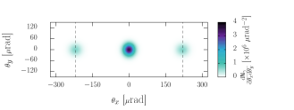
The scattering channels and in Eq. (7) correspond to the case that a photon is absorbed and emitted to the same beam, which by energy momentum conservation gives , (where the sign indicates some allowance for a small spread of momenta due to finite bandwidth effects as explained in the previous paragraph). For these channels the signal photons receive no lateral momentum kick and peak around , along the propagation direction of the probe XFEL beam. Instead, the main interest in the three-beam configuration is in the and , channels of Eq. (7) which includes absorption of photons from one optical beam and emission to the other. This produces Bragg side-peaks outside of the emission cone of the XFEL probe beam, centred around where,
| (25) |
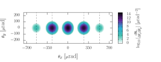
An example of the distribution of scattered photons for currently attainable parameters is shown in Fig. (2). Only two side-peaks are visible, corresponding to 4-photon scattering and in Eq. (23). At the level of the probability, the coupling to each optical field scales as (recall the fields are normalised by the Schwinger critical field strength) and since 6-photon scattering has two extra vertices coupled to optical fields compared with 4-photon scattering, the 6-photon scattering signal is very weak. By momentum conservation in Eq. (23) with there are two further Bragg side peaks and these are demonstrated in Fig. (3) on a logarithmic plot with future parameters for the optical beam. (See Sec. V below for more details on the parameters used.)
IV Determination of fundamental low-energy constants
First we present analytical results that link the number of polarised and unpolarised scattered photons to the fundamental low-energy constants in Eq. (2). To simplify the analysis we set the polarisation plane of the optical beams to be equal, . Then only two polarisation angles remain: for the x-ray polarisation plane and for the optical polarisation plane. We can obtain more manageable expressions for the number of signal photons by considering an expansion of the amplitudes in Eq. (11) for , or equivalently by taking (see Eq. (24)). In fact, expanding only the tensor structure, i.e. in Eq. (9), one finds that the parallel and perpendicular amplitudes can be expressed as
| (26) |
where , , , and depend only on the and the initial beam polarisations, and . Explicitly:
| (27) |
where , and , . The functions and contain all of the spacetime dependent information
| (28) | ||||
and, in general, , since the electric fields are normalised by the critical field. We note here the different dependence of the integral prefactors in and on the collision angle, . On the interval , the prefactor of is a monotonically decreasing function of , with a maximum at . Conversely, the prefactor of peaks around , and vanishes for . This emphasises the fact that the NLO contribution is heavily suppressed in a head-on two-beam collision, and indicates a preferred geometry for the three-beam NLO interaction. Later numerical investigation will confirm the NLO signal peaks at .
Consider now the (differential) number of photons scattered into each of the polarisation modes, Eq. (11). With the tensor structure expanded as before, to leading order in , these will take the form,
| (29) |
These terms contain a dominant contribution from the LO 4-photon interaction, , a term which depends only on the NLO 6-photon interaction, , and an interference term which mixes the LO and NLO contributions, . Since, in general, , any kinematic region in which the contributions from the LO and NLO diagrams overlap will be dominated by the LO process. We first concentrate on determination of the fundamental low-energy constants of LO scattering.
Fundamental constants of 4-photon scattering
Due to the additional suppression of NLO scattering by powers of the critical field, in detector regions where the contributions from LO and NLO scattering overlap the NLO terms in Eq. (IV) can be neglected, giving the simple expressions,
| (30) |
The function contains all of the spacetime structure and integrations which will be strongly depend on the experimental pulse parameters and shot-to-shot fluctuations. The field-independent pre-factors of coincide with known scaling laws found for the case of a two-beam head-on collision, see for example Karbstein et al. (2022), and depend only on the 4-photon low-energy constants Ritus (1975),
| (31) |
and the relative polarisation of the x-ray and optical beams . When , takes its maximum value of ; when , and take their maximum values . There are two different types of measurement that can be performed to determine the fundamental low-energy constants and .
i) Polarisation-sensitive measurement of the number of photons at a fixed angle of polarisation of the XFEL beam. In this case, is fixed and forming the ratio of to , we see:
| (32) |
which is independent of and not effected by experimental factors such as the field-strengths, space-time overlap, or collision angle of the three beams.
ii) Polarisation-insensitive measurement of just the number of scattered photons at two different angles of polarisation of the XFEL beam. In this case, the two angles of polarisation correspond to with a photon count and with a photon count , with the condition . The ratio of these two measurements would also be independent of ,
| (33) |
These two routes to determining the fundamental low-energy constants and have been outlined in the literature for the two-beam case Mosman and Karbstein (2021). However, a clear advantage of the three-beam set-up is that the photons are scattered into side-peaks and hence are spatially separated from the large x-ray background from the probe XFEL beam. This may prove to be more attractive experimentally than modifying the XFEL beam with advanced techniques such as the shadow technique Karbstein et al. (2022).
A further advantage is the choice of XFEL beam mode. X-ray polarimetry, for example using quasi-channel-cut crystals, can set a strict bound on the allowable bandwidth of the x-ray pulse to the order of Ahmadiniaz et al. (2024). If a measurement requires a high level of x-ray polarimetry this limits the mode of the XFEL beam to use a low-bandwidth option such as self-seeding. However, if polarisation-insensitive measurements can be used, such as suggested by the three-beam configuration, there is no strict requirement on the x-ray bandwidth and one can use alternative x-ray modes that offer larger numbers of photons per pulse, such as SASE Kondratenko and Saldin (1980); Bonifacio et al. (1984). Since the total number of signal photons is directly proportional to the number of probe x-ray photons using e.g. the SASE mode can lead to a significant increase in the signal versus a polarisation-sensitive measurement.
Fundamental constants of 6-photon scattering
A highlight of the three-beam configuration is that -photon scattering is separated into different side-peaks for different , see Eq. (25). If the NLO 6-photon side-peak is sufficiently separated from the LO side-peak such that we can neglect the signal from the LO interaction, we find
| (34) |
and the spacetime dependence can be factorised into the integral . Just as in the LO case Eq. (32), we can form the ratio of polarised photons to arrive at a quantity that is relatively insensitive to shot-to-shot variations.
Alongside the 6-photon fundamental low-energy constants Ritus (1975),
| (35) |
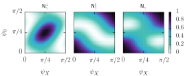
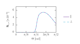
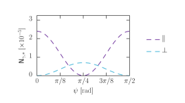
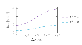
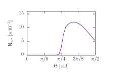
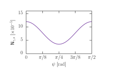
the number of signal photons due to the NLO interaction depends explicitly on the polarisation angles and , rather than just their difference as was the case for the LO interaction Eq. (30). The dependence on the polarisation angles is illustrated in Fig. (4). The reason for this different dependency on the polarisation is due to the configuration of colliding three beams. For the side-peaks, the LO process of 4-photon scattering has a different optical beam connected to the two ‘pump’ vertices, whereas for the NLO process of 6-photon scattering the four ‘pump’ vertices involve the same optical beam being connected to two vertices. This has a restrictive effect on the NLO tensor structure which makes it more sensitive to the beam polarisations.
From Fig. (4) it can be seen that the number of perpendicular-polarised photons is maximised when , but, with this same choice, the number of parallel-polarised photons goes to zero. Likewise, the number of parallel-polarised photons or total number of photons are maximised when or , where the number of perpendicular-polarised photons falls to zero. Making use of the partial symmetry between and , we simplify the analysis by choosing . Using Eq. (IV), we find
| (36) | ||||
This also gives a simple ratio,
| (37) |
V Numerical results
In this section, we present numerical results for the number of scattered photons for two different sets of experimental parameters. We consider a currently attainable case which could be sufficient to measure the LO process of 4-photon scattering and a future parameters case which would allow access to the NLO process of 6-photon scattering. Measurement of the NLO process of 6-photon scattering is currently beyond experimental reach, but would be aided by having a more intense optical laser, higher brilliance XFEL beam, or collisions at a higher repetition rate. The numerical results also act as a test of the analytically-derived expressions relating the fundamental low-energy constants to numbers of polarised and unpolarised scattered photons.
Currently attainable parameters
| Optical | X-ray (Self-seeded) | X-ray (SASE) | ||||||||||
|---|---|---|---|---|---|---|---|---|---|---|---|---|
| [] | [] | [] | [] | [] | [] | [] | [] | [] | [] | |||
| EU.XFEL Ahmadiniaz et al. (2024) | ||||||||||||
| SACLA Yabuuchi et al. (2019); Inoue et al. (2019) | ||||||||||||
| Future | ||||||||||||
For the currently-attainable XFEL beam, technology is assumed that is capable of offering hard x-rays with energy and numbers of photons per pulse . The energy requirement ensures that the photon-photon cross section is enhanced relative to an all-optical configuration while the number of photons per pulse ensures that the number of signal photons, , which scales as , is large enough for a significant number of events to be observed. Also important is the availability of both SASE Kondratenko and Saldin (1980); Bonifacio et al. (1984) and self-seeded Feldhaus et al. (1997); Gianluca Geloni and Saldin (2011) operational modes. For polarisation resolved measurements, the self-seeded injection scheme is the most suitable (i.e. vacuum birefringence experiments), as typical crystal polarimeters have a narrow acceptance bandwidth . For polarisation insensitive measurements, one can instead use the SASE mode which provides a larger number of photons per bunch at the expense of a larger bandwidth. For the currently-attainable optical beams, we assume a peak power and short duration . The number of signal photons, , scales at LO with the optical beam intensity, , as .
Two examples of facilities meeting the above requirements are the European X-ray Free Electron Laser (EU.XFEL) Laso Garcia et al. (2021); Ahmadiniaz et al. (2024) and the SPring-8 Angstrom Compact Free Electron Laser (SACLA) Yabuuchi et al. (2019); Inoue et al. (2019). The EU.XFEL produces coherent pulses with photon energies in the range . These can be combined with the Ti:Sa optical ReLaX laser system installed at the Helmholtz International Beamline for Extreme Fields (HIBEF) Laso Garcia et al. (2021), offering a total pulse energy of at a duration, corresponding to a peak power . The waist is given by , where is the f-number of the focussing optics. Assuming that the ReLaX beamline is passed through a 50:50 beamsplitter to produce two optical pulses with energy , for each pulse can reach an intensity of . The EU.XFEL parameters in Tab. (1) are taken to coincide with those of the proposed BIREF@HIBEF experiment Ahmadiniaz et al. (2024). SACLA offers a similar XFEL capability, providing coherent pulses with photon energies . At SACLA there is also a Ti:Sa optical laser system capable of delivering two duration laser pulses with combined total energy , corresponding to a total peak power Yabuuchi et al. (2019). Assuming the capability to focus each pulse to a beam waist , as for the ReLaX system above, this corresponds to a peak intensity of per pulse. In the following sections we will evaluate the feasibility of performing photon-photon scattering discovery experiments at both EU.XFEL and SACLA.
Future Parameters
Going beyond the constraints of currently available technology we also consider what sort of signals one may expect at next generation facilities. Our goal is to explore the feasibility of using such a set up to access both the LO and NLO photon-photon scattering contributions. The number of signal photons from the NLO contribution will be proportional to , such that there is a strong dependence on the field strength of the optical laser pulses. For this reason, we focus on the interaction of a next generation multi-kJ-class high-power laser system with x-ray pulses. Many x-ray free electron laser facilities which provide high-brightness hard x-ray pulses operate with a similar capability to the EU.XFEL and so we will use these parameters for the x-ray beam as a demonstrative example. For the optical laser, we consider pulses of 30 fs duration generated from a Ti:Sa laser system and capable of reaching an intensity level of . The parameters of such a laser system are outlined in Tab. (1).
V.1 Background estimation
The number of signal photons per optimal collision of the three beams can reach of the order per collision for the ‘currently attainable’ parameters in Tab. (1). The number of x-ray photons per shot is . Although the signal is separated from the background in spatial co-ordinate and polarisation, a good understanding of the background is essential in any experiment. Considering the background also allows one to determine suitable values for the remaining free x-ray and optical beam parameters, namely the x-ray photon energy, , and the x-ray and optical beam waists, and .
The majority of the XFEL photons will be filtered out by placing the detector at the position of the Bragg side-peaks and ensuring those peaks are a suitable distance from the central peak. Consider a detector a distance down the x-ray propagation axis with a circular exclusion region of radius , corresponding to an angular cut . Assuming that the detector can measure all signal photons with , the total number of signal photons will be,
| (38) |
Treating the measurement of the number of scattered photons as Poissonian with a background count per shot of , following Cowan et al. (2011), the number of optimal shots required to reach a statistical significance of using the three-beam scenario is
| (39) |
We identify two potential sources of background for all measurements: the divergence of the x-ray beam, , and Compton scattering from impurities in the vacuum chamber, . Another source of background, effecting only polarisation sensitive measurements, is due to the polarisation purity of the probe x-ray pulse, . The total background is then
| (40) |
The optical elements used to focus the x-ray beam will also impact the number of signal and background photons per shot. Assuming the use of two standard beryllium lenses, one to focus the probe beam and another to focus the signal, each with a transmission, this leads to a total reduction by a factor in the number of signal and background photons.
X-ray beam divergence:
The biggest potential source of background comes from the divergence of the probe x-ray beam. Since , measurements will be background dominated if even a fraction of a percent of probe photons diverge beyond the detector exclusion region. The number of XFEL photons beyond the angular cut can be estimated by integrating , given by Eq. (A), on the detector over time and azimuthal angle:
| (41) |
where is the focussing -number and is the wavelength of the x-rays. If one demands , then:
| (42) |
For the XFEL + optical set-up considered here, and . If we choose for some to fulfil Eq. (42), then a condition on the angular detector cut is:
| (43) |
We expect that when the signal is largest, the centre of the Bragg side peaks will be on the detector, , which also implies . Using Eq. (25) this gives a condition:
| (44) |
These conditions imply a hierarchy for the associated angles, . Considering the standard deviation of an x-ray pulse with , the angular cut must satisfy . Similarly, considering the optical pulse with and a collision angle of , the condition in Eq. (44) sets a lower bound of for the LO contribution with . Thus, a choice of and satisfies the x-ray divergence and Bragg side-peak conditions, and a detector placed down the x-ray beamline will measure background photons from the x-ray beam divergence outside of the exclusion region, such that we can neglect this contribution to the background.
Compton scattering:
Another source of background will be from Compton scattering of x-ray photons and electrons in the interaction vacuum chamber, as in practice a perfect vacuum is not feasible. The interaction geometry of the three-beam setup makes a precise calculation of the background due to Compton scattering a nontrivial task Ahmadiniaz et al. (2022b). However, one can estimate an upper bound on this background in the following way. Given an x-ray pulse with photons in a duration , the number of scattered photons due to Compton scattering can be estimated as , where is the Thomson scattering cross section and is the density of electrons. We assume a vacuum of , corresponding to , which gives . This estimate does not include considerations about the number of these photons which will reach the detectors or the effect of ponderomotive blow out on the electron population, both of which should act to reduce the contribution to the background from Compton scattering (see e.g. Lundstrom et al. (2006) for a similar discussion in the context of colliding three optical pulses). Thus, can be viewed as an upper bound.
X-ray polarisation purity:
For polarisation sensitive measurements we must also consider the effect of the polarisation purity of the probe x-ray beam, , where is the number of photons in the probe pulse which are polarised in the orthogonal polarisation mode. An orthogonally polarised photon in the initial beam scattering without polarisation flip will contribute a background to the measurement, while those photons scattering with polarisation flip will contribute a background to the measurement. While this background could be reduced by using additional polarisers to improve the polarisation purity of the x-ray pulses, these also introduce detrimental effects such as transmission losses and pulse lengthening Karbstein et al. (2021). We will find, below, that the EU.XFEL polarisation purity of without additional polarisers leads to backgrounds that are sufficiently small Geloni et al. (2015). For polarisation insensitive measurements, where only the photon count on the detector is important, the background is a component of the signal itself, and so can be neglected.
V.2 Polarisation-sensitive measurements
V.2.1 Currently available technology: 4-photon scattering
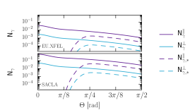
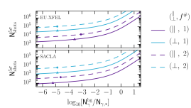
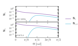
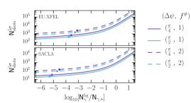
Our goal now is to estimate the number of signal photons which could be obtained in a polarisation sensitive measurement using technology currently available at EU.XFEL and SACLA, using Tab. (1). We consider the scattering of self-seeded photons with optical pulses at () focussing. The remaining free parameters are , and , satisfying the constraints Eq. (42)–(44). The angle between the x-ray and optical polarisation planes is chosen as , maximising the number of x-ray photons scattered into the ‘flipped’ polarisation state, c.f. Eq. (30). The number of signal photons per optimal shot neglecting losses due to x-ray optics is shown in Fig. (5) for both EU.XFEL (upper panel) and SACLA (lower panel) parameters with focussing of the optical pulses. Choosing an angular cut , the dashed lines in Fig. (5) show the number of parallel () and perpendicular () polarised photons with scattering angles , peaking at a collision angle with and for EU.XFEL parameters and at with and for SACLA parameters.
The number of background photons of any polarisation due to Compton scattering is determined as for the EU.XFEL parameters and for SACLA parameters. The number of background photons in a specific polarisation can be acquired by considering x-ray pulse polarisation purity, Geloni et al. (2015), giving for the Compton parallel polarisation background, and for the Compton perpendicular polarisation background. This corresponds to for the EU.XFEL and for SACLA. For polarisation sensitive measurements we also have to estimate the direct contribution to the background from the polarisation purity. For the total number of x-ray photons per pulse of , there are probe photons in the orthogonal polarisation mode. The contribution to the background from these photons depends on the pulse parameters and configuration. Considering the collision at which approximately maximises the signals for photons with for EU.XFEL and SACLA parameters, we find the polarisation purity contributes and background photons to, respectively, the parallel and perpendicular EU.XFEL measurements, and and background photons to the SACLA measurements. Thus, the main contribution to the parallel polarisation background is from Compton scattering, while the polarisation purity of the probe is the dominant background factor of the perpendicular measurement. Including the effect of focussing optics by reducing the signal and background contributions by a factor , the detected photon counts are given in Tab. (2). Using these in Eq. (39) we can estimate the number of optimal shots which would be required to achieve a statistical significance of in a polarisation sensitive measurement. For EU.XFEL parameters we find and , while for SACLA parameters we find and . Since the parallel and perpendicular photons can be measured simultaneously in a single shot, the total number of required shots to obtain significance in both observables will be determined by , which is also shown in Tab. (2).
| EU.XFEL | 1 | ||||||
|---|---|---|---|---|---|---|---|
| 2 | |||||||
| SACLA | 1 | ||||||
| 2 |
While we have provided estimates and chosen suitable parameters to minimise the background contributions for idealised shots, we have not taken into account experimental fluctuations. The estimates of the number of shots required for a given will be sensitive to the actual background which is measured in each shot. When more factors are taken into account, the level of the background in experiment may take different values than considered here. Therefore, it is useful to understand how the projected number of required shots changes with the background, for the estimated number of signal photons in Tab. (2). In Fig. (6) the number of shots required for a statistical significance of is calculated according to Eq. (39) as a function of the ratio . Since the number of signal photons in each case is fixed to the estimates in Tab. (2), the increase in corresponds to an increase in the background. The data points correspond to the background estimations in Tab. (2).
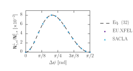
In Sec. IV it was shown that the ratio of polarised scattered photons, , is independent of the spacetime overlap of the beams. Determining the ratio allows the fundamental QED low-energy constants to be inferred. This conclusion is supported by the numerical result in Fig. (7), which calculates this ratio numerically and finds the same result as the analytical prediction Eq. (31). This also confirms the dependency of the ratio of polarised photons on the angle between the x-ray and optical polarisation planes from Eq. (32).
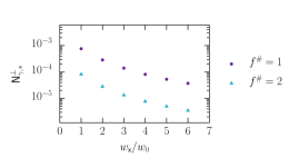
In experiment it may be advantageous to increase the x-ray and optical beam-overlap (for example to minimise the effect of beam jitter), which can be achieved by defocussing the optical laser. Since the number of polarisation-flipped photons , where is the intensity of the corresponding field changing the optical f-number from to , naïvely results in the intensity change and the reduction in the number of signal photons by over a magnitude . However, if is kept fixed and , the reduction due to the increase in will be partially compensated by more probe photons being within the foci of the optical pulses. Fig. (8) shows how the birefringence signal depends on the relative overlap of the x-ray and optical beams, which can be quantified by the ratio , using EU.XFEL parameters. Overall, we see for fixed , doubling leads to around an order of magnitude reduction in . For fixed , going from to results in around an order of magnitude decrease in the number of scattered photons.
V.2.2 Next generation technology: 6-photon scattering
With each power of the electric field strength in in Eq. (2) there is also an additional suppression by the critical field strength, . Therefore, the measurable photons mostly originate from the LO process; when attempting to isolate the NLO process, the LO process becomes a source of background. One tool which we can use to aid with separating the contributions is the angular cut on the detector. The Bragg peaks corresponding to the NLO interaction are centered around , which is twice as far from the origin as the LO Bragg peak, see Eq. (25). Thus, we expect that a larger angular cut (which will turn out to be around twice the cut used in the preceding section) can be taken to isolate the signal from the NLO interaction on the detector. This has an additional effect of allowing us to choose a smaller beam waist for the x-ray pulses, , while still ensuring that the background due to its divergence is negligible and the conditions Eq. (41)–(44) are satisfied. Correspondingly, in the following we choose and . The remaining parameters for the x-ray and optical lasers are given in Tab. (1), where we choose focussing for the optical lasers.
Consider now the birefringent signal. To determine the fundamental constants using Eq. (36) for a fixed polarisation angle of the x-ray and optical beams, both the number of parallel-polarised and perpendicular-polarised photons must be measured. We saw from Fig. (4) that as the optical and x-ray polarisation plane angle, , is varied, the number of photons scattered into the perpendicular polarisation mode is maximised where the number in the parallel mode vanishes and vice versa. To determine a suitable value for , we pick the value at which the ratio . From Eq. (37), this occurs when
| (45) |
where the approximated values are those obtained using Eq. (35). For other choices of , one of or will be smaller, making measurement more difficult. The choice of is selected for Fig. (9), which shows the number of signal photons in each polarisation mode. The number of parallel polarised photons with .
As expected from our choice of , we find that the number of parallel and perpendicular polarised photons coincide, peaking around with the value . Following the same analysis as in the preceding section of estimating the background per shot and taking into account the x-ray optics, we find,
|
|
(46) |
which amounts to and . While the number of shots is perhaps prohibitively large for a birefringent measurement to be feasible using the proposed parameters, particularly since the high pulse energy requirement of the optical pulses would likely mean a low repetition rate, we emphasise that the number of signal photons is directly proportional to the number of XFEL photons, . We have considered here a next generation high-power laser combined with an XFEL with currently available technology. Thus, it is possible that advances in XFEL technology could push the birefringent signal to a viable level for detection in an experiment.
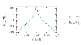
Before moving on to consider the polarisation insensitive case we consider how the ratio varies for the NLO contribution. Choosing the collision angle which maximises the birefringent signal of photons with in Fig. (9), we plot in Fig. (11) the ratio Eq. (37) with Eq. (35) (black solid) against the numerically evaluated ratio. We find perfect agreement between the two cases.
V.3 Polarisation-insensitive measurements
V.3.1 Currently available technology: 4-photon scattering
We now consider measurement of the unpolarised process. One advantage of a polarisation insensitive measurement is that the SASE mode of the XFEL can be used, which increases the number of photons per bunch (see Tab. (1)). From Eq. (30) and Eq. (31) it is clear that the total number of signal photons is maximised when the difference in polarisation angle, . In this case the number of perpendicular polarised photons drops to zero (see Eq. (30)). The dependence of the total number of signal photons versus the collision angle is shown in Fig. (12) for focussing with EU.XFEL (upper panel) and SACLA (lower panel) SASE parameters. The solid lines show the total number of signal photons with all scattering angles, , i.e. including those in the central peak (see Fig. (2)). Since the signal photons are purely parallel polarised, the photons in the central peak will of course be indistinguishable from the background probe XFEL photons, and so the dashed lines show the total number of signal photons with angles , . This peaks at the collision angle with for EU.XFEL parameters, and with for SACLA. The combination of the increase in the number of probe photons, , and the use of the polarisation difference leads to almost an order of magnitude increase in the number of signal photons per shot with comparison to the polarisation sensitive measurements, Fig. (5).
To enable the determination of the experimental values of the 4-photon low-energy constants and it is necessary to perform at least two independent measurements. For the polarisation sensitive measurement of Sec. V.2.1 these were the number of photons scattered into the parallel and perpendicular polarisation modes. For a polarisation insensitive measurement, where only the total number of signal photons is obtained, the two independent observables must come from measurements at different choices of the relative angle of the XFEL and optical polarisation planes, . How the number of signal photons varies with for fixed collision angle is shown in Fig. (13) for EU.XFEL parameters. Unlike in the polarisation sensitive measurement, where the difference in the number of parallel and perpendicular signal photons per shot is over an order of magnitude, the difference between a measurement at and is only around a factor of . This means that each measurement will require a comparable number of shots to reach a particular statistical significance and, coupled with the higher number of signal photons per shot, the total required shots to determine and will be less than in the polarisation sensitive case.
| EU.XFEL | 1 | |||||
|---|---|---|---|---|---|---|
| 2 | ||||||
| SACLA | 1 | |||||
| 2 |
We again wish to estimate the minimum number of shots required to obtain a statistical significance, . With the background from the x-ray divergence and the polarisation purity playing no role, the main source of background in the polarisation insensitive measurement will be from Compton scattering, , which is estimated as for EU.XFEL parameters and for SACLA parameters. Accounting for the reduction of both the signal and background by the x-ray optics, the number of signal photons for different measurements and optical focussing are presented in Tab. (3). Taking the independent observables to be the measurements at at optical focussing, these estimates correspond to and for EU.XFEL parameters, and and for SACLA parameters. The total number of shots required to measure both observables will be the sum , which are also shown in Tab. (3). Comparing with Tab. (2) we see that over an order of magnitude fewer shots would be required to determine the experimental values of the fundamental low energy constants and to statistical significance. This is also seen in Fig. (14), which shows how the number of shots required for significance in the polarisation insensitive measurement varies with the background using the estimated number of signal photons from Tab. (3).
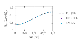
When considering the birefringent signal, it was possible to demonstrate through Fig. (7) that the ratio of the number of perpendicular to parallel polarised signal photons follow simple analytical relationships which depend only on the fundamental low-energy constants of the LO process and the polarisation difference, Eq. (32). We can demonstrate an analogous relationship in the polarisation insensitive measurement by instead considering the ratio of the total number of signal photons due to different polarisation differences, , see Eq. (33). This is shown in Fig. (15) for a fixed collision angle of for optical focussing. We take as a reference value the number of signal photons at , , and use this to normalise the number of photons as a function of , . This normalisation ensures that all of the spacetime dependent factors cancel, and we see that the simple analytical ratio Eq. (33) agrees with the numerically evaluated data for both EU.XFEL (purple circles) and SACLA (blue triangles) SASE parameters.
V.3.2 Next generation technology: 6-photon scattering
We now consider a measurement of unpolarised photon-photon scattering with an upgraded optical laser Tab. (1) as in Sec. V.2.2 (with , , ). The polarisation is chosen to optimise the number of scattered photons: . Fig. (16) shows the dependence of the total number of signal photons with , , on the collision angle at fixed . The use of SASE parameters has increased the number of photons with to a peak of at . While still small, this is a large improvement over the polarisation sensitive measurement outlined in Sec. V.2.2.
Just as in the LO case, we need two independent measurements to be able to experimentally determine the values of the 6-photon low-energy constants, theoretically predicted as in Eq. (35). The two observables are chosen as the total number of signal photons at two different values of the polarisation parameter . The dependence of the total number of signal photons on is shown in Fig. (17). We have chosen the collision angle around which the number of signal photons has a maximum in Fig. (16). In this case we find, including the effect of x-ray focussing optics,
|
|
(47) |
with the estimated backgrounds being the same as in the preceding section. We estimate that shots would be required to determine the 6-photon low-energy constants to significance.
VI Summary
Real photon-photon scattering has yet to be experimentally verified. Measuring either the unpolarised or the polarised case (vacuum birefringence) would allow confirmation of an outstanding prediction from quantum electrodynamics (QED) for the magnitude of fundamental low-energy constants that govern the effective nonlinear coupling of photons with one other. Measurement of the effective photon-photon coupling could be used to place bounds on new physics beyond the Standard Model Ahlers et al. (2008); Gies (2009); Villalba-Chávez et al. (2017, 2016); Fouché et al. (2016); Beyer et al. (2020); Ejlli et al. (2020); Evans and Schützhold (2024) and act as a gateway to harnessing the nonlinear vacuum for more exotic applications such as vacuum high harmonic generation and self-focussing.
We have shown that there are several advantages in using a planar three-beam set-up to measure photon-photon scattering. The kinematics allow for photons to be scattered into Bragg side-peaks in the detector plane, thereby providing spatial separation of the signal from the large photon background and significantly increasing the signal-to-noise ratio compared to the more conventional two-beam set-up. In the planar three-beam set-up: i) the fundamental low-energy QED constants can be determined by measuring numbers of scattered photons, without the need for polarimetry; ii) since the bandwidth of the x-ray beam does not have to be especially low for polarimetry purposes, an XFEL seeding mode such as SASE can be used that increases the photon-photon scattering signal; iii) higher orders of photon-photon scattering lead to further Bragg side-peaks that correlate transverse detector position with expansion order of the effective photon-photon interaction. This in principle allows the determination of fundamental low-energy QED constants for higher dimensional terms that lead to e.g. six-photon scattering. These considerations further emphasise the point that configurations of lasers that are beyond plane waves can support processes that are otherwise kinematically suppressed in the plane wave case.
Specifically, we calculated the number of scattered photons if an XFEL provides the probe field and two high power optical beams provide the pump field. Two different parameter sets were considered. Firstly, currently available technology was shown to be sufficient to measure 4-photon scattering; parameters were chosen from those available at the EU.XFEL, which will be used in the proposed BIREF@HIBEF experiment Schlenvoigt et al. (2016); Ahmadiniaz et al. (2024), and those available at SACLA. We found that the number of required shots to obtain a significance value using the three-beam scenario, c.f. Tab. (2) and Tab. (3), could be competitive with, and/or complementary to, other approaches such as the dark-field method Karbstein et al. (2022); Ahmadiniaz et al. (2024). Secondly, we considered future technology to measure 6-photon scattering with the EU.XFEL and an optical laser capable of reaching intensities of , such as may be achievable at the Station of Extreme Light Shen et al. (2018). Alternatively, future parameters to increase the 6-photon signal could involve increasing the brilliance of the XFEL beam or the frequency of collisions with the optical beams.
Acknowledgments
AJM is supported by the project “Advanced Research Using High Intensity Laser Produced Photons and Particles” (ADONIS) CZ.02.1.01/0.0/0.0/16_019/0000789 from European Regional Development Fund (ERDF). The authors thank Sergei V. Bulanov for useful discussions.
Appendix A Beam field profiles
In this appendix we give more details about the field profiles of the three input beams to our configuration. The XFEL beam and the two optical beams are all described by Gaussian focussed pulses in the paraxial approximation. The normalised electric field profiles, , are,
| (48) |
where is the curvature parameter defined in terms of the Rayleigh length , with defined as the distance from the focus at which the peak intensity is reduced by a factor , and , the 3-wavevector of . The phase duration of the pulses is , with the temporal duration at which the pulse intensity falls to of the peak. The field strengths can be expressed in terms of the total energy of the pulse as Karbstein and Mosman (2017),
| (49) |
where for simplicity we consider both the optical lasers to have the same field strength and, waist, and duration, is the number of photons in the x-ray pulse and is the energy of the optical pulses. The coordinates denote the directions transverse to the beam propagation direction. With the wavevectors outlined in Sec. III, the transverse coordinates are, for ,
| (50) |
for ,
| (51) |
and for ,
| (52) |
The signal photons, , are taken to be plane wave states,
| (53) |
with
| (54) |
and a volumetric normalisation.
Numerical results presented in Sec. V have primarily been obtained using the “infinite Rayleigh length approximation” (IRLA), where in Eq. (A) King et al. (2010a); King and Keitel (2012); Gies et al. (2018b); King et al. (2018); Karbstein et al. (2021). In the planar three-beam collision considered in this paper, the functional dependence of the beam profiles Eq. (A) mean that the temporal and out-of-plane coordinate integrals in Eq. (5) and (9) can be performed analytically, as they are Gaussian. However, with the IRLA the form of the beam profiles simplify considerably,
| (55) |
allowing all of the coordinate integrals in Eq. (5) and (9) to be performed analytically. In Fig. (18) we show the relative error
between the number of signal photons calculated with the full Gaussian pulses in the paraxial approximation Eq. (A), , and the IRLA Eq. (55), . The purple lines correspond to the currently available parameters EU.XFEL parameters used in Fig. (12), with the solid line for all signal photons and the dashed line for only photons within the acceptance region of the detector with . The blue dashed line is for the number of photons on the detector acceptance region using the future parameters from Fig. (16). We find that for the case of including all signal photons the IRLA agrees very well with the results using the full Gaussian pulse in the paraxial approximation, with across the full range of the collision angle . When the detector cut is included, for both currently available and future parameters, we find that for collision angles the error becomes quite large, but as the collision angle increases this rapidly falls to the level of . This can be understood by considering what happens when the collision angle is increased from . Initially, the Bragg side-peaks are emitted head-on and are excluded by the detector cut. As is increased, the centre of the Bragg side-peaks move to larger and eventually to values large enough for their outer edges to fall on the detector. To describe the side-peak edges accurately, wavefront curvature and the Gouy phase must be included, so for these values of , where the signal is low, the IRLA makes a significant error. By experimenting turning on and off various terms in the paraxial beam Eq. (A), it can be confirmed that the main error is made when both the wavefront curvature and the Gouy terms in the phase are neglected in this cut side-peak region. Once the collision angle is increased further so that the Bragg side-peak signal is fully on the detector, the error in the IRLA falls to a very low value. Most importantly, at the collision angle which maximises for the currently available parameters, (vertical dashed lines), and for the future parameters, (vertical dotted lines), the relative error is on the level of and , respectively.

References
- Sauter (1931) F. Sauter, Z. Phys. 69, 742 (1931).
- Halpern (1933) O. Halpern, Phys. Rev. 44, 855.2 (1933).
- Heisenberg (1934) W. Heisenberg, Z. Phys. 90, 209 (1934), english translation: Remarks on the Dirac theory of the positron, in A. I. Miller, Early Quantum Electrodynamics, pp. 169-187, Cambridge UP, 1995. [Erratum: Z.Phys. 92, 692–692 (1934)].
- Heisenberg and Euler (1936) W. Heisenberg and H. Euler, Z. Phys. 98, 714 (1936), arXiv:physics/0605038 .
- Schwinger (1951) J. S. Schwinger, Phys. Rev. 82, 664 (1951).
- Toll (1952) J. S. Toll, (1952), phD thesis, Princeton.
- Delbrück (1933) M. Delbrück, Z. Phys. 84, 144 (1933).
- Schumacher et al. (1975) M. Schumacher, I. Borchert, F. Smend, and P. Rullhusen, Phys. Lett. B 59, 134 (1975).
- Aaboud et al. (2017) M. Aaboud et al. (ATLAS), Nature Phys. 13, 852 (2017), arXiv:1702.01625 [hep-ex] .
- Aad et al. (2019) G. Aad et al. (ATLAS), Phys. Rev. Lett. 123, 052001 (2019), arXiv:1904.03536 [hep-ex] .
- Sirunyan et al. (2019) A. M. Sirunyan et al. (CMS), Phys. Lett. B 797, 134826 (2019), arXiv:1810.04602 [hep-ex] .
- Brandenburg et al. (2023) J. D. Brandenburg, J. Seger, Z. Xu, and W. Zha, Rept. Prog. Phys. 86, 083901 (2023), arXiv:2208.14943 [hep-ph] .
- Adam et al. (2021) J. Adam et al. (STAR), Phys. Rev. Lett. 127, 052302 (2021), arXiv:1910.12400 [nucl-ex] .
- Di Piazza et al. (2006) A. Di Piazza, K. Z. Hatsagortsyan, and C. H. Keitel, Phys. Rev. Lett. 97, 083603 (2006), arXiv:hep-ph/0602039 .
- King et al. (2010a) B. King, A. Di Piazza, and C. H. Keitel, Nature Photon. 4, 92 (2010a), arXiv:1301.7038 [physics.optics] .
- King et al. (2010b) B. King, A. Di Piazza, and C. H. Keitel, Phys. Rev. A 82, 032114 (2010b), arXiv:1301.7008 [physics.optics] .
- Kryuchkyan and Hatsagortsyan (2011) G. Y. Kryuchkyan and K. Z. Hatsagortsyan, Phys. Rev. Lett. 107, 053604 (2011).
- Tommasini and Michinel (2010) D. Tommasini and H. Michinel, Phys. Rev. A 82, 011803 (2010), arXiv:1003.5932 [hep-ph] .
- Monden and Kodama (2011) Y. Monden and R. Kodama, Phys. Rev. Lett. 107, 073602 (2011).
- King and Keitel (2012) B. King and C. H. Keitel, New J. Phys. 14, 103002 (2012), arXiv:1202.3339 [hep-ph] .
- Jin et al. (2022) B. Jin, B. Shen, and D. Xu, Phys. Rev. A 106, 013502 (2022).
- Gies et al. (2013) H. Gies, F. Karbstein, and N. Seegert, New J. Phys. 15, 083002 (2013), arXiv:1305.2320 [hep-ph] .
- Lundstrom et al. (2006) E. Lundstrom, G. Brodin, J. Lundin, M. Marklund, R. Bingham, J. Collier, J. T. Mendonca, and P. Norreys, Phys. Rev. Lett. 96, 083602 (2006), arXiv:hep-ph/0510076 .
- Gies et al. (2014) H. Gies, F. Karbstein, and R. Shaisultanov, Phys. Rev. D 90, 033007 (2014), arXiv:1406.2972 [hep-ph] .
- Aboushelbaya et al. (2019) R. Aboushelbaya et al., Phys. Rev. Lett. 123, 113604 (2019), arXiv:1902.05928 [physics.optics] .
- Formanek et al. (2024) M. Formanek, J. P. Palastro, D. Ramsey, S. Weber, and A. Di Piazza, Phys. Rev. D 109, 056009 (2024), arXiv:2307.11734 [hep-ph] .
- Jin and Shen (2023) B. Jin and B. Shen, Phys. Rev. A 107, 062213 (2023).
- Berezin and Fedotov (2024) A. V. Berezin and A. M. Fedotov, (2024), arXiv:2405.00151 [hep-ph] .
- Valialshchikov et al. (2024) M. Valialshchikov, F. Karbstein, D. Seipt, and M. Zepf, (2024), arXiv:2405.03317 [hep-ph] .
- Rozanov (1993) N. N. Rozanov, Zhurnal Eksperimentalnoi i Teoreticheskoi Fiziki 103, 1996 (1993).
- Di Piazza et al. (2005) A. Di Piazza, K. Z. Hatsagortsyan, and C. H. Keitel, Phys. Rev. D 72, 085005 (2005).
- Fedotov and Narozhny (2007) A. Fedotov and N. Narozhny, Physics Letters A 362, 1 (2007).
- Heyl and Hernquist (1999) J. S. Heyl and L. Hernquist, Phys. Rev. D 59, 045005 (1999), arXiv:hep-th/9811091 .
- Böhl et al. (2015) P. Böhl, B. King, and H. Ruhl, Phys. Rev. A 92, 032115 (2015), arXiv:1503.05192 [physics.plasm-ph] .
- Marklund and Shukla (2006) M. Marklund and P. K. Shukla, Rev. Mod. Phys. 78, 591 (2006).
- Di Piazza et al. (2012) A. Di Piazza, C. Müller, K. Z. Hatsagortsyan, and C. H. Keitel, Rev. Mod. Phys. 84, 1177 (2012).
- King and Heinzl (2016) B. King and T. Heinzl, High Power Laser Sci. Eng. 4 (2016), 10.1017/hpl.2016.1, arXiv:1510.08456 [hep-ph] .
- Fedotov et al. (2022) A. Fedotov, A. Ilderton, F. Karbstein, B. King, D. Seipt, H. Taya, and G. Torgrimsson, (2022), arXiv:2203.00019 [hep-ph] .
- Weber et al. (2017) S. Weber et al., Matter Radiat. Extremes 2, 149 (2017).
- Shen et al. (2018) B. Shen, Z. Bu, J. Xu, T. Xu, L. Ji, R. Li, and Z. Xu, Plasma Phys. Control. Fusion 60, 044002 (2018).
- Danson et al. (2019) C. N. Danson et al., High Power Laser Science and Engineering 7, e54 (2019).
- Xu et al. (2020) D. Xu, B. Shen, J. Xu, and Z. Liang, Nuclear Instruments and Methods in Physics Research Section A: Accelerators, Spectrometers, Detectors and Associated Equipment 982, 164553 (2020).
- Piazza et al. (2022) A. D. Piazza, L. Willingale, and J. D. Zuegel, “Multi-petawatt physics prioritization (mp3) workshop report,” (2022), arXiv:2211.13187 [hep-ph] .
- Dinu et al. (2014a) V. Dinu, T. Heinzl, A. Ilderton, M. Marklund, and G. Torgrimsson, Phys. Rev. D 89, 125003 (2014a), arXiv:1312.6419 [hep-ph] .
- Dinu et al. (2014b) V. Dinu, T. Heinzl, A. Ilderton, M. Marklund, and G. Torgrimsson, Phys. Rev. D 90, 045025 (2014b), arXiv:1405.7291 [hep-ph] .
- Bragin et al. (2017) S. Bragin, S. Meuren, C. H. Keitel, and A. Di Piazza, Phys. Rev. Lett. 119, 250403 (2017), arXiv:1704.05234 [hep-ph] .
- Meuren et al. (2015) S. Meuren, K. Z. Hatsagortsyan, C. H. Keitel, and A. Di Piazza, Phys. Rev. Lett. 114, 143201 (2015), arXiv:1407.0188 [hep-ph] .
- King and Elkina (2016) B. King and N. Elkina, Phys. Rev. A 94, 062102 (2016), arXiv:1603.06946 [hep-ph] .
- Macleod et al. (2023) A. J. Macleod, J. P. Edwards, T. Heinzl, B. King, and S. V. Bulanov, New J. Phys. 25, 093002 (2023), arXiv:2304.02114 [hep-ph] .
- Moulin and Bernard (1999) F. Moulin and D. Bernard, Optics Communications 164, 137 (1999).
- Lundin et al. (2006) J. Lundin, M. Marklund, E. Lundstrom, G. Brodin, J. Collier, R. Bingham, J. T. Mendonca, and P. Norreys, Phys. Rev. A 74, 043821 (2006), arXiv:hep-ph/0606136 .
- Gies et al. (2018a) H. Gies, F. Karbstein, C. Kohlfürst, and N. Seegert, Phys. Rev. D 97, 076002 (2018a), arXiv:1712.06450 [hep-ph] .
- King et al. (2018) B. King, H. Hu, and B. Shen, Phys. Rev. A 98, 023817 (2018), arXiv:1805.03688 [hep-ph] .
- Ahmadiniaz et al. (2022a) N. Ahmadiniaz, T. E. Cowan, J. Grenzer, S. Franchino-Viñas, A. L. Garcia, M. Smid, T. Toncian, M. A. Trejo, and R. Schützhold, (2022a), arXiv:2208.14215 [physics.optics] .
- Fouché et al. (2016) M. Fouché, R. Battesti, and C. Rizzo, Phys. Rev. D 93, 093020 (2016), [Erratum: Phys.Rev.D 95, 099902 (2017)], arXiv:1605.04102 [physics.optics] .
- Karbstein et al. (2022) F. Karbstein, D. Ullmann, E. A. Mosman, and M. Zepf, Phys. Rev. Lett. 129, 061802 (2022), arXiv:2207.09866 [hep-ph] .
- Ejlli et al. (2020) A. Ejlli, F. Della Valle, U. Gastaldi, G. Messineo, R. Pengo, G. Ruoso, and G. Zavattini, Phys. Rept. 871, 1 (2020), arXiv:2005.12913 [physics.optics] .
- Schulze et al. (2022) K. S. Schulze, B. Grabiger, R. Loetzsch, B. Marx-Glowna, A. T. Schmitt, A. L. Garcia, W. Hippler, L. Huang, F. Karbstein, Z. Konôpková, H.-P. Schlenvoigt, J.-P. Schwinkendorf, C. Strohm, T. Toncian, I. Uschmann, H.-C. Wille, U. Zastrau, R. Röhlsberger, T. Stöhlker, T. E. Cowan, and G. G. Paulus, Phys. Rev. Res. 4, 013220 (2022).
- Kondratenko and Saldin (1980) A. Kondratenko and E. Saldin, Part. Accel. 10, 207 (1980).
- Bonifacio et al. (1984) R. Bonifacio, C. Pellegrini, and L. Narducci, Optics Communications 50, 373 (1984).
- Berestetskii et al. (1982) V. B. Berestetskii, E. M. Lifshitz, and L. P. Pitaevskii, QUANTUM ELECTRODYNAMICS, Course of Theoretical Physics, Vol. 4 (Pergamon Press, Oxford, 1982).
- De Tollis (1965) B. De Tollis, Nuovo Cim. 35, 1182 (1965).
- Huang and Kim (2007) Z. Huang and K.-J. Kim, Phys. Rev. ST Accel. Beams 10, 034801 (2007).
- McNeil and Thompson (2010) B. W. McNeil and N. R. Thompson, Nature photonics 4, 814 (2010).
- Pellegrini et al. (2016) C. Pellegrini, A. Marinelli, and S. Reiche, Rev. Mod. Phys. 88, 015006 (2016).
- Feng and Deng (2018) C. Feng and H.-X. Deng, Nuclear Science and Techniques 29, 160 (2018).
- Huang et al. (2021) N. Huang, H. Deng, B. Liu, D. Wang, and Z. Zhao, The Innovation 2 (2021).
- Heinzl et al. (2006) T. Heinzl, B. Liesfeld, K.-U. Amthor, H. Schwoerer, R. Sauerbrey, and A. Wipf, Opt. Commun. 267, 318 (2006), arXiv:hep-ph/0601076 .
- Karbstein et al. (2015) F. Karbstein, H. Gies, M. Reuter, and M. Zepf, Phys. Rev. D 92, 071301 (2015), arXiv:1507.01084 [hep-ph] .
- Schlenvoigt et al. (2016) H.-P. Schlenvoigt, T. Heinzl, U. Schramm, T. E. Cowan, and R. Sauerbrey, Phys. Scripta 91, 023010 (2016).
- Inada et al. (2017) T. Inada, T. Yamazaki, T. Yamaji, Y. Seino, X. Fan, S. Kamioka, T. Namba, and S. Asai, Science 7, 671 (2017), arXiv:1707.00253 [hep-ex] .
- Shakeri et al. (2017) S. Shakeri, S. Z. Kalantari, and S.-S. Xue, Phys. Rev. A 95, 012108 (2017), arXiv:1703.10965 [hep-ph] .
- Huang et al. (2019) S. Huang, B. Jin, and B. Shen, Phys. Rev. D 100, 013004 (2019).
- Seino et al. (2020) Y. Seino, T. Inada, T. Yamazaki, T. Namba, and S. Asai, PTEP 2020, 073C02 (2020), arXiv:1912.01390 [hep-ph] .
- Schmitt et al. (2021) A. T. Schmitt et al., Optica 8, 56 (2021), arXiv:2003.00849 [physics.ins-det] .
- Karbstein et al. (2021) F. Karbstein, C. Sundqvist, K. S. Schulze, I. Uschmann, H. Gies, and G. G. Paulus, New J. Phys. 23, 095001 (2021), arXiv:2105.13869 [hep-ph] .
- Yu et al. (2023) Q. Yu, D. Xu, B. Shen, T. E. Cowan, and H.-P. Schlenvoigt, High Power Laser Science and Engineering 11, e71 (2023).
- Wang et al. (2024) J. Wang, G. Y. Chen, B. F. Lei, S. Jin, L. Y. Yang, L. F. Gan, C. T. Zhou, S. P. Zhu, X. T. He, and B. Qiao, New J. Phys. 26, 023008 (2024).
- Galtsov and Skobelev (1971) D. Galtsov and V. Skobelev, Physics Letters B 36, 238 (1971).
- Ritus (1975) V. Ritus, J. Exp. Theor. Phys. 42, 774 (1975).
- Mosman and Karbstein (2021) E. A. Mosman and F. Karbstein, Phys. Rev. D 104, 013006 (2021), arXiv:2104.05103 [hep-ph] .
- Ahmadiniaz et al. (2024) N. Ahmadiniaz et al., (2024), arXiv:2405.18063 [physics.ins-det] .
- Yabuuchi et al. (2019) T. Yabuuchi, A. Kon, Y. Inubushi, T. Togahi, K. Sueda, T. Itoga, K. Nakajima, H. Habara, R. Kodama, H. Tomizawa, et al., Journal of synchrotron radiation 26, 585 (2019).
- Inoue et al. (2019) I. Inoue, T. Osaka, T. Hara, T. Tanaka, T. Inagaki, T. Fukui, S. Goto, Y. Inubushi, H. Kimura, R. Kinjo, et al., Nature photonics 13, 319 (2019).
- Feldhaus et al. (1997) J. Feldhaus, E. Saldin, J. Schneider, E. Schneidmiller, and M. Yurkov, Optics Communications 140, 341 (1997).
- Gianluca Geloni and Saldin (2011) V. K. Gianluca Geloni and E. Saldin, Journal of Modern Optics 58, 1391 (2011), https://doi.org/10.1080/09500340.2011.586473 .
- Laso Garcia et al. (2021) A. Laso Garcia, H. Höppner, A. Pelka, C. Bähtz, E. Brambrink, S. Di Dio Cafiso, J. Dreyer, S. Göde, M. Hassan, T. Kluge, and et al., High Power Laser Science and Engineering 9, e59 (2021).
- Cowan et al. (2011) G. Cowan, K. Cranmer, E. Gross, and O. Vitells, Eur. Phys. J. C 71, 1554 (2011), [Erratum: Eur.Phys.J.C 73, 2501 (2013)], arXiv:1007.1727 [physics.data-an] .
- Ahmadiniaz et al. (2022b) N. Ahmadiniaz, T. E. Cowan, M. Ding, M. A. L. Lopez, R. Sauerbrey, R. Shaisultanov, and R. Schützhold, (2022b), arXiv:2212.03350 [hep-ph] .
- Geloni et al. (2015) G. Geloni, V. Kocharyan, and E. Saldin, Optics Communications 356, 435 (2015).
- Ahlers et al. (2008) M. Ahlers, H. Gies, J. Jaeckel, J. Redondo, and A. Ringwald, Phys. Rev. D 77, 095001 (2008), arXiv:0711.4991 [hep-ph] .
- Gies (2009) H. Gies, Eur. Phys. J. D 55, 311 (2009), arXiv:0812.0668 [hep-ph] .
- Villalba-Chávez et al. (2017) S. Villalba-Chávez, T. Podszus, and C. Müller, Phys. Lett. B 769, 233 (2017), arXiv:1612.07952 [hep-ph] .
- Villalba-Chávez et al. (2016) S. Villalba-Chávez, S. Meuren, and C. Müller, Phys. Lett. B 763, 445 (2016), arXiv:1608.08879 [hep-ph] .
- Beyer et al. (2020) K. A. Beyer, G. Marocco, R. Bingham, and G. Gregori, Phys. Rev. D 101, 095018 (2020), arXiv:2001.03392 [hep-ph] .
- Evans and Schützhold (2024) S. Evans and R. Schützhold, Phys. Rev. D 109, L091901 (2024), arXiv:2307.08345 [hep-ph] .
- Karbstein and Mosman (2017) F. Karbstein and E. A. Mosman, Phys. Rev. D 96, 116004 (2017), arXiv:1711.06151 [hep-ph] .
- Gies et al. (2018b) H. Gies, F. Karbstein, and C. Kohlfürst, Phys. Rev. D 97, 036022 (2018b), arXiv:1712.03232 [hep-ph] .