Fast and Accurate GHZ Encoding Using All-to-all Interactions

Abstract

The $N$-qubit Greenberger–Horne–Zeilinger (GHZ) state is an important resource for quantum technologies. We consider the task of GHZ encoding using all-to-all interactions, which prepares the GHZ state in a special case, and is furthermore useful for quantum error correction and enhancing the rate of qubit interactions. The naive protocol based on parallelizing CNOT gates takes $\mathrm{O}(1)$-time of Hamiltonian evolution. In this work, we propose a fast protocol that achieves GHZ encoding with high accuracy. The evolution time $\mathrm{O}(\log^{2}N/N)$ almost saturates the theoretical limit $\Omega(\log N/N)$. Moreover, the final state is close to the ideal encoded one with high fidelity $>1-10^{-3}$, up to large system sizes $N\lesssim 2000$. The protocol only requires a few stages of time-independent Hamiltonian evolution; the key idea is to use the data qubit as control, and to use fast spin-squeezing dynamics generated by e.g. two-axis-twisting.

Introduction.— Quantum technologies offer great possibilities to perform information processing tasks far more efficiently than classical machines. For example, quantum computers are potentially able to factorize large numbers Shor (1999) or solve linear systems of equations Harrow et al. (2009) exponentially fast. As of estimating unknown parameters, quantum metrology can achieve a Heisenberg-limited precision that surpasses classical resources Giovannetti et al. (2004), using entangled states like the Greenberger–Horne–Zeilinger (GHZ) state Greenberger et al. (1989) and spin-squeezed states Kitagawa and Ueda (1993); Ma et al. (2011); Bornet et al. (2023); Eckner et al. (2023); Franke et al. (2023). By far, quantum computation and squeezing physics are rather disconnected: Although squeezing implies entanglement Korbicz et al. (2005, 2006), one usually does not care about the precise form of the squeezed state in the many-body Hilbert space: one merely uses a single parameter to describe the squeezing strength, which is sufficient to infer the ultimate precision in metrology Ma et al. (2011). In contrast, quantum computation aims to produce precise states/unitaries from which one can deduce e.g. the precise factors of a large number. As a result, quantum computation is usually modeled by digitized quantum circuits, instead of analog Hamiltonian evolution that is more suitable for squeezing.

However, quantum circuits may not exploit the full power of current quantum platforms, because many of them are naturally equipped by Hamiltonians with high connectivity: Rydberg atoms interact with strength $r^{-\gamma}$ that decays as a power law with distance $r$, where the exponenent $\gamma=3,6$ Browaeys and Lahaye (2020). Moreover, all-to-all interactions

$$H(t)=\sum_{i<j}J_{ij}^{ab}(t)X^{a}_{i}X^{b}_{j},\quad{\rm where}\quad\left\lvert J_{ij}^{ab}(t)\right\rvert\leq 1,$$ (1)

arise in optical cavities Li et al. (2023); Cooper et al. (2024), almost in trapped ions with $\gamma\in[0,3]$ Britton et al. (2012); Monroe et al. (2021), and are proposed for superconducting circuits Pita-Vidal et al. (2024). With such Hamiltonian, a single qubit interacts with many others simultaneously, which potentially enhances the information processing speed. This is particularly demanding in the current noisy intermediate-scale quantum (NISQ) era, where one wants to perform computation faster than the decoherence timescale, when useful information would be lost into the environment. Indeed, for any power-law exponent $\gamma<2d+1$, protocols have been constructed that transmit quantum information through space in a way that is asymptotically faster than local quantum circuits/ Hamiltonians in $d$ spatial dimensions Tran et al. (2020, 2021a); Hong and Lucas (2021). For $\gamma>d$, there are also lower bounds on the protocol time that matches the fast protocols Chen and Lucas (2019); Kuwahara and Saito (2020); Tran et al. (2020, 2021b); see the recent review Chen et al. (2023). However, such speed limits are much less understood for $\gamma<d$, where the system is closer to the all-to-all limit. Here, the notion of spatial locality is challenged by a diverging local energy density; although progress have been made regarding Frobenius operator growth Lucas (2020); Yin and Lucas (2020); Kuwahara and Saito (2021), this is not directly related to tasks of e.g. preparing a certain entangled state.

In this work, we focus on the all-to-all setting of $N+1$ qubits $i\in\Lambda:=\{0,1,\cdots,N\}$, and propose an efficient protocol for GHZ encoding: For any quantum state $\alpha\ket{0}+\beta\ket{1}$ with $\left\lvert\alpha\right\rvert^{2}+\left\lvert\beta\right\rvert^{2}=1$ originally contained in the data qubit $i=0$, the protocol generates a unitary $U$ that encodes the quantum data into the GHZ subspace of all qubits:

$$U\ket{\alpha,\beta;0}\approx\ket{\alpha,\beta},\quad\forall\alpha,\beta$$ (2)

where

$$\ket{\alpha,\beta;0} :=\left(\alpha\ket{0}+\beta\ket{1}\right)_{0}\otimes\ket{\bm{0}},$$ (3a)

$$\ket{\alpha,\beta} :=\alpha\ket{\bm{0}}_{\Lambda}+\beta\ket{\bm{1}}_{\Lambda}.$$ (3b)

Here $\ket{\bm{0}}$ ($\ket{\bm{0}}_{\Lambda}$) is the all-zero state on qubits $\{1,\cdots,N\}$ (all qubits $\Lambda$), and $\ket{\bm{1}}$ is the all-one state similarly. To the best of our knowledge, the previous fastest protocol (including approximate ones, as we use “$\approx$” in (2) and will quantify the error shortly) is to apply Hamiltonian $H=Z_{0}(X_{1}+\cdots+X_{N})$ for time $T=\pi/4=\Theta(1)$ , before locally rotating all $i>0$ by $\mathrm{e}^{-\mathrm{i}\pi X_{i}/4}$. Here we assume local rotations are arbitrarily fast and not counted in the total evolution time, since they do not change entanglement, and are usually much faster than qubit interactions in reality Browaeys and Lahaye (2020); Monroe et al. (2021). Alternatively, this exact protocol can be viewed as applying CNOT gates in parallel, where the data qubit $i=0$ controls all other qubits. However, there is a large gap between this constant runtime and the known lower bound using an all-to-all possibly time-dependent Hamiltonian $H(t)$ (1):

$$T=\Omega(\log N/N),$$ (4)

which vanishes quickly with $N$. See Supplemental Material (SM) for the proof of (4), which is adapted from Chen et al. (2023), and also holds for approximate protocols with $\mathrm{O}(1)$ infidelity (defined in (6) below). After all, the above protocol only uses $\mathrm{O}(N)$ out of $\Theta(N^{2})$ pairs of interactions in $H(t)$.

In contrast, our protocol almost saturates the bound, where $H(t)$ is applied for time

$$T=\mathrm{O}(\log^{2}N/N).$$ (5)

This is the first protocol with such a small runtime $T=\tilde{\mathrm{O}}(1/N)$ for any digital quantum information processing task . Our main idea is to generate many-body entanglement using fast spin-squeezing protocols like two-axis-twisting (TAT) Kitagawa and Ueda (1993); Luo et al. (2024); Miller et al. (2024), which generates an extremely-squeezed state in short time $T=\tilde{\mathrm{O}}(1/N)$. Although the squeezing subroutines make our protocol inexact, we carefully design “unsqueezing” stages that cancel the unwanted squeezing effects with high precision, bridging the gap between analog and digital quantum evolution. Remarkably, the error is very small for all system sizes $N\lesssim 2000$ studied numerically, quantified by

$$\epsilon:=1-\min_{\alpha,\beta}\left\lvert\bra{\alpha,\beta}U\ket{\alpha,\beta;0}\right\rvert^{2},$$ (6)

i.e. the worst-case infidelity of $U\ket{\alpha,\beta;0}$ with respect to the target state $\ket{\alpha,\beta}$. We have $\epsilon<10^{-3}$ when the numerical coefficient in (5) is $\approx 1$, and can be further improved by increasing $T$ systematically.

Implications.— Before describing our protocol in detail, we first discuss its implications. In the special case $\alpha=\beta=1/\sqrt{2}$, our protocol prepares the GHZ state with high fidelity. GHZ state generation have been studied extensively, in both recent experimental demonstrations with $N\sim 20$ Monz et al. (2011); Pogorelov et al. (2021); Wang et al. (2018); Zhong et al. (2018); Song et al. (2019); Mooney et al. (2021); Omran et al. (2019); Cao et al. (2024), and theoretical proposals beyond parallelizing CNOT gates Ho et al. (2019); Alexander et al. (2020); Zhao et al. (2021); Comparin et al. (2022a); Wang et al. (2023); Zhang et al. (2023, 2024). However, all existing protocols either take long evolution time like parallelizing CNOTs, or produce GHZ-like states, whose fidelity with the true GHZ state is not as high as ours ($\epsilon<10^{-3}$) at large $N\gtrsim 10^{3}$. For example, Zhang et al. (2024) proposes a $T=\mathrm{O}(\log N/N)$ protocol using all-to-all interactions that prepares a GHZ-like state of the form $c_{0}\left(\ket{D^{N}_{0}}+\ket{D^{N}_{N}}\right)/\sqrt{2}+c_{1}\left(\ket{D^{N}_{1}}+\ket{D^{N}_{N-1}}\right)/\sqrt{2}+\cdots$. Here $\ket{D^{N}_{k}}$ is the Dicke state that is the equal superposition of all computational basis states with $k$ ones and $N-k$ zeros (so $(\ket{D^{N}_{0}}+\ket{D^{N}_{N}})/\sqrt{2}$ is the GHZ state), so that the GHZ-like state corresponds to $\epsilon=1-\left\lvert c_{0}\right\rvert^{2}\approx 0.65$ for $N=100$. This protocol has several drawbacks: (1) Since it is only GHZ-like, although it has nearly maximal quantum Fisher information Giovannetti et al. (2004) for sensing $Z$ field like the ideal GHZ state, it is in general unclear how to saturate this metrological limit by an efficient measurement strategy Yin and Lucas (2024). (2) The protocol requires the coupling coefficients $J(t)$ to change very fast in time, in order to engineer an effective $3$-local Hamiltonian from Magnus expansion. (3) Most importantly, it only prepares one state and does not achieve GHZ encoding for any $\alpha,\beta$. Indeed, the protocol Hamiltonian in Zhang et al. (2024) is invariant when permuting the qubits, so does not map the state on a particular qubit to global one like (2). Nevertheless, the spin-squeezing idea in Zhang et al. (2024) inspired our work, which overcomes the above challenges, by e.g. using the data qubit as control for (3).

Beyond preparing GHZ states, our protocol can be used to enhance the interaction rate between two qubits. More concretely, consider two copies of the original setup, where one wants to engineer a gate between two qubits $0,0^{\prime}$, and the rest $2N$ qubits in $\Lambda\cup\Lambda^{\prime}$ are in the all-zero state. One can first apply our protocol $U_{\Lambda}\otimes U_{\Lambda^{\prime}}$ to encode each of them into the GHZ subspace of a qubit ensemble of size $\sim N$, and then the two ensembles can interact with a strength $\sum_{i\in\Lambda,j\in\Lambda^{\prime}}Z_{i}Z_{j}\sim N^{2}\gg 1$ due to their large polarizations. By reversing the GHZ encoding procedure (i.e. uncomputing) and adding fast single-qubit rotations, this implements an arbitrary two-qubit gate in time $2T+\mathrm{O}(1/N^{2})=\tilde{\mathrm{O}}(1/N)$. This is much faster than applying the gate directly on the two qubits. The gate error $\sim\epsilon/N$ is also vanishingly small, because as we will see, the $\alpha$-part $\psi$ of our encoded state, for example, has polarization $\left\langle\sum_{i}Z_{i}\right\rangle_{\psi}=N-\mathrm{O}(\epsilon)$ with relative error $\mathrm{O}(\epsilon/N)$, where we have defined $\left\langle\mathcal{O}\right\rangle_{\psi}:=\left\langle\psi|\mathcal{O}|\psi\right\rangle$.

The GHZ subspace can be viewed as a quantum error correction (QEC) code that corrects bit-flip errors with maximal distance $N+1$, mimicking the classical repetition code. This is called spin-cat code in Omanakuttan et al. (2024). Concatenating spin-cat codes as in the Shor code Shor (1995) also corrects phase errors, leading to a high threshold for quantum fault-tolerance Omanakuttan et al. (2024). Our protocol can be used to encode/decode such QEC codes in a fast way, where decoherence errors do not have much time to accumulate during the process. On the other hand, there may also exist “gate” errors due to imprecise control in the protocol, and a small change $\delta T\sim 1/N$ in evolution time is already detrimental. As a result, there is a tradeoff between these different error types, and one may want to optimize over $N$ and other parameters, when implementing our protocol in reality.

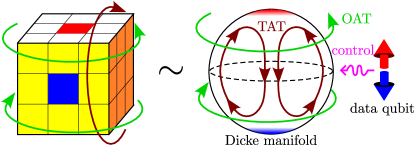
Figure 1: Our GHZ encoding protocol (right) shares the similar spirit of the Rubik’s Cube (left), where intriguing color patterns are obtained by composing a set of basic operations. The quantum problem consists of $N$ qubits supporting a Dicke manifold, and one qubit originally containing the quantum data. GHZ encoding (sketched by the red/blue colors) is achieved by a finite round of fast basic operations, including interaction between the two subsystems, and unitaries on the Dicke manifold from OAT/TAT.

The protocol and building blocks.— Our GHZ encoding unitary $U$ involves several stages composed of simple subroutines:

$$U=S_{\tau_{3}}\left(R^{Z}_{\pi/4}O_{\pi/4}R^{X}_{-\pi/2}\right)S_{-\tau_{2}}\,\left(C_{\phi}\,S_{\tau_{1}}\right),$$ (7)

where $\tau_{p}\,(p=1,2,3)$ and $\phi$ are parameters that we tune and optimize. The high-level idea of (7) is analogous to Rubik’s Cube, as shown in Fig. 1: we first identify the basic operations, and then decompose complicated tasks into them. In our problem, the GHZ encoding task is decomposed to basic operations that are fast to implement, e.g. local rotations and squeezing dynamics. Here, we first introduce the building blocks in (7), and describe the whole protocol later.

The unitaries appeared in (7) are defined by

$$R^{X^{a}}_{\phi}: =\mathrm{e}^{\mathrm{i}\frac{\phi}{2}X^{a}}.$$ (8a)

$$C_{\phi}: =\mathrm{e}^{\mathrm{i}\frac{\phi}{2}Z_{0}\otimes X},$$ (8b)

$$S_{\tau}: =\mathrm{e}^{-\mathrm{i}\tau\frac{\log N}{N}H_{\rm TAT}},$$ (8c)

$$O_{\phi}: =\mathrm{e}^{-\mathrm{i}\frac{\phi}{4N}Z^{2}},$$ (8d)

where $H_{\rm TAT}=XY+YX$, and $X^{a}:=\sum_{i=1}^{N}X^{a}_{i}$ (excluding site $0$), which are also denoted by $X,Y,Z$ for $a=1,2,3$ respectively. We explain the unitaries one by one, where it is useful to consider them as acting on the Dicke manifold $\mathrm{Span}(\ket{D^{N}_{k}}:k=0,1,\cdots,N)$, which at $N\rightarrow\infty$ becomes a semiclassical phase space: a sphere.

The simplest (8a) is just rotation of angle $\phi$ around the $a$-axis. For example, if $a=3$, $R^{Z}_{\phi}$ rotates from east to west in the Dicke manifold, where we set $Z=N$ as the north pole.

(8b) is controlled $X$-rotation, i.e. depending on whether the control qubit $i=0$ is in $\ket{0}$ or $\ket{1}$, the other qubits are rotated by angle $\phi$ either clockwise or counterclockwise. This is the only building block that acts nontrivially on qubit $0$.

(8c) is the TAT Hamiltonian/unitary, which generates spin squeezing (the symbol $S$ stands for “squeezing”) for initial product state $\ket{\bm{0}}$. In particular, at rescaled time $\tau=\tau_{\rm min}\approx 1/8$ Liu et al. (2011), the squeezing is extreme (i.e. asymptotically optimal):

$$\frac{\left\langle\Delta Y\right\rangle_{\Psi}}{\left\langle Z\right\rangle_{\Psi}}=\Theta\left(\frac{1}{N}\right),$$ (9)

where $\ket{\Psi}=S_{\tau_{\rm min}}\ket{\bm{0}}$ is the final state, and $\left\langle\Delta Y\right\rangle_{\Psi}:=\sqrt{\left\langle Y^{2}\right\rangle_{\Psi}-\left\langle Y\right\rangle_{\Psi}^{2}}$. The ratio (9) is much smaller than that $\Theta(1/\sqrt{N})$ for the initial spin-coherent state $\ket{\bm{0}}$. This squeezing dynamics can be understood in the semiclassical Dicke manifold: Define the normalized angular momentum $X^{a}_{\rm cl}:=X^{a}/N$, which satisfy commutation relation

$$[X_{\rm cl},Y_{\rm cl}]=N^{-2}[X,Y]=N^{-2}2\mathrm{i}Z=:2\mathrm{i}\hbar Z_{\rm cl},$$ (10)

where $\hbar:=1/N$ is the effective Planck constant (the other two commutators are in a similar form). Then $S_{\tau}=\mathrm{e}^{-\mathrm{i}(\tau\log N)H_{\rm cl}/\hbar}$ where

$$H_{\rm cl}:=X_{\rm cl}Y_{\rm cl}+Y_{\rm cl}X_{\rm cl}\approx 2X_{\rm cl}Y_{\rm cl},$$ (11)

can be viewed as a classical Hamiltonian on the unit-sphere phase space if $\hbar\ll 1$, i.e. $N\gg 1$. In this semiclassical limit, roughly speaking, the initial state $\ket{\bm{0}}$ corresponds to an ensemble of initial points near the north pole $Z_{\rm cl}=1$, and the evolved state $\ket{\Psi}$ corresponds to the ensemble of these points evolved by the classical trajectories of $H_{\rm cl}$. It turns out that $Z_{\rm cl}=1$ is a saddle point in phase space, so the ensemble is squeezed exponentially in the $Y$ (and minus $Y$) direction, and stretched exponentially in the $X$ direction. Since the initial ensemble has width $\Delta Y_{\rm cl}\sim 1/\sqrt{N}$, the extreme squeezing $\Delta Y_{\rm cl}\sim 1/N$ is achieved when $\mathrm{e}^{-\lambda(\tau\log N)}\times 1/\sqrt{N}\approx 1/N$, which leads to (9) because the Lyapunov exponent at the saddle point is $\lambda=4$.

(8d) is the one-axis twisting (OAT) unitary Kitagawa and Ueda (1993) ($O$ stands for “one”) that also generates squeezing for initial product states polarized near the equator $Z\approx 0$. However, this squeezing property is not what we will use in our protocol. Instead, we interpret $O_{\phi}$ as a relative rotation that rotates the north and south semispheres in opposite directions. In particular, near the north pole the rotation is from west to east with angle $\phi$, while near the south pole it is east to west with angle $\phi$.

Combining building blocks.— We express the bare controlled-rotation angle $\phi$ by a normalized parameter $\theta$:

$$\phi=\theta\left(\log^{2}N\right)/N.$$ (12)

As we will see, the parameters $\tau_{p},\theta$ do not scale with $N$, so the total time $T$ of our protocol (7) is dominated by the controlled-rotation $\theta$:

$$T=\theta\frac{\log^{2}N}{2N}+\frac{\pi}{8N}+\frac{\log N}{N}\sum_{p=1,2,3}\tau_{p}\approx\theta\frac{\log^{2}N}{2N},$$ (13)

at sufficiently large $N$, where the rotations $R$ are assumed to be instantaneous.

We have combined the subroutines into four logical stages in (7), and we present the ideas for them one by one:

1. Squeeze-to-separate $C_{\phi}\,S_{\tau_{1}}$: The ultimate goal of GHZ encoding $\ket{\alpha,\beta}=\alpha\ket{0}_{0}\otimes\ket{\bm{0}}+\beta\ket{1}_{0}\otimes\ket{\bm{1}}$ can be interpreted as, depending on the state of the control qubit $0$, the polarization of the rest qubits are either very positively polarized or very negatively polarized. In other words, the two parts ($\alpha$-part and $\beta$-part) of the state are “supported” in faraway regions on the Dicke manifold of the $N$ qubits. Since the two parts have the same initial support $\ket{\bm{0}}$ around the north pole, the first thing to do is to separate their supports to disjoint regions, before pulling the two supports faraway from each other. The naive way to separate is just a controlled rotation like $C_{\phi}$: $C_{\phi}\left(\alpha\ket{0}+\beta\ket{1}\right)_{0}\otimes\ket{\bm{0}}=\alpha\ket{0}_{0}\otimes\ket{\bm{\phi}}+\beta\ket{1}\otimes\ket{\bm{-\phi}}$; see Hosten et al. (2016) for similar ideas. However, the product states $\ket{\bm{\pm\phi}}$ have quantum fluctuations of size $\Delta Y\sim\sqrt{N}$, so they have disjoint support on the size-$N$ Dicke manifold only after $\phi\gtrsim 1/\sqrt{N}$, which would lead to $T\gtrsim 1/\sqrt{N}$ in the end.

Our idea here for $C_{\phi}\,S_{\tau_{1}}$ is to first squeeze the state using TAT to reduce the quantum fluctuation along $y$-axis, and then controlled-rotate. See Fig 2(a), where the red initial state is squeezed to the orange one, and then evolved to the green ones. Naively, at $\tau_{1}=\tau_{\rm min}\approx 1/8$ the squeezing is extreme $\Delta Y\sim 1$, so rotation angle

$$\phi\sim(\log N)/N,\quad\quad\text{(naive)}$$ (14)

suffices. Here the $\log N$ factor is such that the distance between the two supports is $\log N$-times larger than their fluctuation width, so that their overlap is inverse-polynomially small in $N$ (assuming the decay over distance is Gaussian for example). However, we add one more factor of $\log N$ in (12). The reason is that at extreme squeezing, the wave packet is also extremely stretched along the perpendicular direction: $\Delta X\sim N$, and it is hard to refocus such an expanded wave packet back to spin-coherent states (the final goal is just superposition of two spin-coherent states!). Therefore, we desire $\tau_{1}<\tau_{\rm min}$ so that the state has not evolved to extreme squeezing. In this case, numerics in SM shows that $\Delta Y\sim\log N$ for nonvanishing but small $\left\lvert\tau-\tau_{\rm min}\right\rvert$. Therefore, the angle (12) needs to be $\log N$ times larger than the naive (14).

2. Pulling-away $S_{-\tau_{2}}$: Having separated the wave packets to disjoint regions on the Dicke manifold based on the control qubit $0$, we then pull the two regions far away from each other until they become antipodal on the sphere. This can be done in a fast way again using the saddle point structure of TAT. Focusing on the centers of the two green regions in Fig. 2(a), they are initially separated in the $y$ direction with distance $\approx 2N\phi$, so we want to reverse the direction of the TAT dynamics in the first stage to stretch the $y$ direction. After time $\tau_{2}>0$, the evolution $S_{-\tau_{2}}$ maps the two wave-packet centers to the $Y=\pm N$ antipodal points, while the two states become squeezed in the $x$ direction, as shown by blue in Fig. 2(a). From the semiclassical analysis above, $\tau_{2}$ is roughly determined by $\theta$: $\mathrm{e}^{\lambda(\tau_{2}\log N)}\times N\phi\approx cN$, so that

$$\tau_{2}\approx\frac{\log(c/\phi)}{4\log N}=\frac{\log(cN/\theta)-2\log(\log N)}{4\log N}.$$ (15)

Here the constant $c=\Theta(1)$ is a subdominant contribution, which comes from the the fact that the exponential acceleration behavior $\mathrm{e}^{\lambda\tau\log N}$ gets modified away from the saddle point.

Figure 2: (a,b) Sketch of our GHZ encoding protocol on the $N$-qubit Dicke manifold, with the first stages in (a) and latter stages in (b). The colors represent different stages. For example, the red shaded circle represents the initial state $\ket{\bm{0}}$, which is evolved by $S_{\tau_{1}}$ to the orange shaded oval representing a squeezed state. After a controlled rotation the wave function separates to two parts shown by solid ($\alpha$-part) or dashed ($\beta$-part) borderlines, corresponding to the control qubit being $\ket{0}$ or $\ket{1}$. The black lines show classical trajectories induced by $H_{\rm TAT}$ with positive $\tau$. States at the boundary of the shown semisphere, like the blue states, have parts outside the boundary, which should be thought of as folding onto the other semisphere. As shown in the upper-right, (a) and (b) are viewing from different directions, and the final (blue) stage of (a) is rotated by $R^{X}_{-\pi/2}$ to get the first (blue) stage of (b). The two red circles in (b) represent the final state that approximately achieves GHZ encoding. (c) Husimi Q function of the state on the Dicke-manifold at different stages in our protocol, from numerics with parameters $(N,\theta,\tau_{1},\tau_{2},\tau_{3})=(1024,2,0.0505,0.111,0.0357)$. Starting from the third plot, the distribution is shown separately for the two parts using red($\alpha$) and blue($\beta$). More precisely, the color (red$\rightarrow$green$\rightarrow$blue) quantifies $Q_{\alpha}-Q_{\beta}$ (positive$\rightarrow 0\rightarrow$negative) with $Q_{\alpha}$ being the Husimi Q function for the $\alpha$-part $\ket{\psi}$. The final state achieves GHZ encoding with infidelity $\epsilon\approx 6.7\times 10^{-4}$.

3. Rotations $R^{Z}_{\pi/4}O_{\pi/4}R^{X}_{-\pi/2}$: We then rotate the two antipodal points to north and south poles by $R^{X}_{-\pi/2}$, so that we have already arrived at a GHZ-like encoded state where the two parts of the state are squeezed states instead of spin-coherent ones like $\ket{\bm{0}}$. It remains to “unsqueeze” them. However, we cannot use TAT directly, because if it unsqueezes the state at the north pole for example, it will further squeeze the south pole state. This is because the two states are both squeezed in the $x$ direction, while the TAT squeezing has different squeezing directions at the two poles, as one can see from the blue states and black trajectories in Fig. 2(b) . Therefore, before unsqueezing, we first relatively-rotate the two states by $\pi/2$ using $O_{\pi/4}$ (blue $\rightarrow$ green), and then rotate by $R^{Z}_{\pi/4}$ to align them back to the $x,y$ directions (green $\rightarrow$ orange).

4. Unsqueeze $S_{\tau_{3}}$: Finally, after aligning the two states with the TAT trajectories, we unsqueeze them by $S_{\tau_{3}}$ with an optimal $\tau_{3}$. Although the final unsqueezed states are not perfect $\ket{\bm{0}},\ket{\bm{1}}$, they are expected to be very close to the perfect ones because their support can be made very close to a circle region of minimal size, as shown by red in Fig. 2(b).

Performance of the protocol.— To demonstrate the above ideas and quantify the performance, we simulate the dynamics numerically up to large system size $N=2048$, enabled by the fact that the state of the $N$ qubits is constrained in the $(N+1)$-dimensional Dicke manifold. Furthermore, we only need to evolve the $\alpha$-part of the state, because the two parts are related by a $\pi$-rotation symmetry of our protocol; see SM. Denoting the final state as $\alpha\ket{0}_{0}\otimes\ket{\psi}+\beta\ket{1}_{0}\otimes\cdots$, the overlap between the $\alpha$-part $\ket{\psi}$ and $\ket{\bm{0}}$ gives the infidelity for GHZ encoding:

$$\epsilon=1-\left\lvert\left\langle\bm{0}|\psi\right\rangle\right\rvert^{2}.$$ (16)

For a given $N$, we sweep the parameter regime $\tau_{1},\tau_{2}\in[0,0.15],\theta\in[0,2]$, and for each set of these parameters, we numerically optimize $\tau_{3}\in[0,0.15]$ in the last unsqueezing stage, to maximize the overlap $\left\lvert\left\langle\bm{0}|\psi\right\rangle\right\rvert$.

For a typical set of parameters with $N=1024,\theta=2$ and $\tau_{p}$s optimized, we show in Fig. 2(c) the wave function at the different stages in the protocol, represented by the Husimi distribution on the $N$-qubit Dicke manifold. The behaviors indeed match the cartoon picture Fig. 2(a,b). Moreover, the infidelity is tiny $\epsilon<10^{-3}$! Putting numbers in (13) yields $T=0.048$ for this parameter set, which is only $\sim 6\%$ of the parallelizing-CNOTs protocol with $T=\pi/4$.

Figure 3: Performance of our protocol. For each set of $N,\theta,\tau_{1}$, we optimize $\tau_{2},\tau_{3}$ to get the data. (a) $\log_{10}\epsilon$ as a function of $\theta$ and $\tau_{1}$ for $N=1024$. (b) Solid (dashed) lines: Fixing $\theta=1$ ($\theta=2$), $\epsilon$ as a function of $\tau_{1}$, where different color represents different $N$ (same below), as shown in the legend. The function is minimum at $\tau_{1}=\tau_{1}(\theta,N)$. (c) With $\tau_{1}$ fixed to the optimal value $\tau_{1}(\theta,N)$, $\epsilon$ decays exponentially with $\theta$. (d) The support (17) of the $\alpha$-part $\ket{\psi}$ over Dicke states decays with $k$ exponentially, where solid (dashed) lines are still for $\theta=1$ ($\theta=2$), and $\tau_{1}=\tau_{1}(\theta,N)$ is optimized.

We then study how the performance of our protocol depends on the parameters. We first verify that the smallest infidelity indeed happens when $\tau_{2}$ is close to the predicted value (15), determined by $\theta,N$ with $c\approx 2$; see SM, where we also report the optimized values for $\tau_{3}$. Fig. 3 then shows the dependence on the remaining parameters $N,\theta,\tau_{1}$, where $\tau_{2},\tau_{3}$ have been optimized accordingly. For a given $N$ and $\theta$, there exists an optimal squeezing time $\tau_{1}=\tau_{1}(\theta,N)$. With $N$ fixed, Fig. 3(a) shows that $\tau_{1}(\theta,N)$ decreases with increasing $\theta$ with a slower and slower slope. The intuition is that for a smaller $\tau_{1}$, i.e. less squeezing in the first stage, the controlled-rotation angle needs to be larger to fully separate the two wave packets; if $\tau_{1}$ is too small $\ll 1$, the $N$-scaling of $\phi$ in (12) would be insufficient, and in the extreme case $\phi=\pi/2$ we return to the parallelizing-CNOT protocol without squeezing.

At fixed $\theta$, Fig. 3(b) shows that $\tau_{1}(\theta,N)$ drifts to larger values when $N$ increases. We expect this to be a finite-size effect, because $\tau_{1}$ is upper bounded by $\tau_{\rm min}$ anyway where squeezing is extreme. The infidelity at $\tau_{1}(\theta,N)$ also slowly increases with $N$, and it is unclear from the finite-size numerics whether it would saturate at some $<1$ value at $N\rightarrow\infty$. Therefore, our protocol is not asymptotically exact, i.e. $\epsilon$ as a function of $N$ does not tends to zero for a fixed $\theta$. Nevertheless, Fig. 3(c) shows that the infidelity decays exponentially when increasing $\theta$, so one can adjust $\theta$ a little bit to compensate the infidelity increase with $N$. Intuitively, this exponential decay with $\theta$ is because the error comes from the fact that the unsqueezing stage cannot cancel the previous squeezing effects perfectly; at larger $\theta$, a smaller squeezing $\tau_{1}$ is sufficient and is easier to cancel. In Fig. 3(d), we also plot the distribution of the $\alpha$-part $\ket{\psi}$ over Dicke states $\ket{D^{N}_{k}}$:

$$\left\lVert P_{\leq k}\ket{\psi}\right\rVert^{2}:=\sum_{\ell=0}^{k}\left\lvert\left\langle D^{N}_{\ell}|\psi\right\rangle\right\rvert^{2},$$ (17)

showing an exponential decay of support on Dicke states with large $k$. As a result, when using our protocol to enhance qubit interactions, the logical error vanishes $\sim\epsilon/N$ with $N$ as advertised, because $\left\lVert P_{\leq 0}\ket{\psi}\right\rVert^{2}=1-\epsilon$, so that $\ket{\psi}$ has polarization $\left\langle Z\right\rangle_{\psi}=\sum_{k}(N-k)\left(\left\lVert P_{\leq k}\ket{\psi}\right\rVert^{2}-\left\lVert P_{\leq k-1}\ket{\psi}\right\rVert^{2}\right)=N-\mathrm{O}(\epsilon)$.

Conclusion.— In this work, we propose a fast and accurate protocol (7) for GHZ encoding using all-to-all interactions, opening up the potential for QEC and interaction enhancement in (NISQ) quantum devices. The protocol uses the data qubit to control rotation on the Dicke manifold of the other qubits, and exploits fast squeezing/unsqueezing dynamics to generate structured entanglement in a timescale $\tilde{\mathrm{O}}(1/N)$ that vanishes quickly with $N$. The encoding error is quantitatively small from numerical simulation, and can be systematically improved by increasing the protocol time.

For future directions, it is interesting to see whether fine-tuning the time-dependence of $H(t)$ can further improve the fidelity: Given that the error of our protocol is already small, we conjecture the existence of a protocol with similar time (5), and an infidelity $\epsilon$ that vanishes at large $N$. This may require a more systematic semiclassical theory for dynamics on the Dicke manifold, where one controls the shape of the wave packet more carefully to achieve a high quantum fidelity (16). Our all-to-all protocol may also be generalized to power-law interactions with exponent $\gamma<d$, which potentially transmits information in a way much faster than existing protocols designed for $\gamma>d$ Tran et al. (2020, 2021a); Hong and Lucas (2021). Recent developments on spin squeezing in such systems Perlin et al. (2020); Comparin et al. (2022b); Block et al. (2023) would be useful.

Acknowledgements.— We thank Andrew Lucas, David T. Stephen and Haoqing Zhang for valuable discussion. This work was supported by the Department of Energy under Quantum Pathfinder Grant DE-SC0024324.

Supplementary Material: Fast and Accurate GHZ Encoding Using All-to-all Interactions

S1 Proof of the lower bound

Proposition 9.3 in Chen et al. (2023) derives the lower bound Eq. (4) in the main text for exact protocols $\epsilon=0$; it is straightforward to generalize the proof to approximate cases:

Theorem 1 (adapted from Chen et al. (2023)).

For any constant $\delta>0$, GHZ encoding with infidelity

$$\epsilon=1/2-\delta,$$ (S1)

requires

$$T=\Omega\left(\frac{\log(\delta N)}{N}\right).$$ (S2)

Proof.

Chen et al. (2023) proves that (S2) is necessary for

$$\left\lVert[UX_{0}U^{\dagger},Z_{1}]\right\rVert\geq 4\delta,$$ (S3)

so we only need to show that any GHZ encoding protocol with (S1) satisfies (S3).

Define projector $P_{\alpha,\beta}:=\ket{\alpha,\beta;0}\bra{\alpha,\beta;0}$. By direct computation, we have

$$\bra{-\beta,\alpha}UX_{0}U^{\dagger}Z_{1}\ket{\alpha,\beta} =\bra{-\beta,\alpha}U\left[P_{-\beta,\alpha}+(1-P_{-\beta,\alpha})^{2}\right]X_{0}U^{\dagger}\ket{\alpha,-\beta}$$

$$=\bra{-\beta,\alpha}U\ket{-\beta,\alpha;0}\bra{\alpha,-\beta;0}U^{\dagger}\ket{\alpha,-\beta}+\bra{-\beta,\alpha}U(1-P_{-\beta,\alpha})X_{0}(1-P_{\alpha,-\beta})U^{\dagger}\ket{\alpha,-\beta},$$ (S4)

where we have used $1-P_{-\beta,\alpha}=(1-P_{-\beta,\alpha})^{2}$ for the projector in the first line. Similarly,

$$\bra{-\beta,\alpha}Z_{1}UX_{0}U^{\dagger}\ket{\alpha,\beta} =-\bra{\beta,\alpha}U\left[P_{\beta,\alpha}+(1-P_{\beta,\alpha})^{2}\right]X_{0}U^{\dagger}\ket{\alpha,\beta}$$

$$=-\bra{\beta,\alpha}U\ket{\beta,\alpha;0}\bra{\alpha,\beta;0}U^{\dagger}\ket{\alpha,\beta}-\bra{\beta,\alpha}U(1-P_{\beta,\alpha})X_{0}(1-P_{\alpha,\beta})U^{\dagger}\ket{\alpha,\beta}.$$ (S5)

Subtracting the above two equations and choosing $\alpha=1,\beta=0$ so that the two first terms are opposite, we have

$$\left\lvert\bra{0,1}[UX_{0}U^{\dagger},Z_{1}]\ket{1,0}\right\rvert \geq 2\left\lvert\bra{0,1}U\ket{0,1;0}\bra{1,0;0}U^{\dagger}\ket{1,0}\right\rvert-2\left\lVert(1-P_{0,1})U\ket{0,1}\right\rVert^{2}$$

$$\geq 2(1-\epsilon)-2\epsilon=2(1-2\epsilon)=4\delta,$$ (S6)

where we have used the definition of $\epsilon$ in the main text Eq. (6). This establishes (S3) and thus (S2). ∎

S2 Symmetry of the protocol

Write the protocol $U$ by $U=U_{\rm later}U_{\rm sep}$ where $U_{\rm sep}=C_{\phi}S_{\tau_{1}}$, and $U_{\rm later}$ is the later stages in Eq. (7) in the main text. Since $U_{\rm sep}(\ket{z}_{0}\otimes\ket{\bm{0}})=\ket{z}_{0}\otimes U_{\mathrm{sep},z}\ket{\bm{0}}$ ($z=0,1$) where the two $z$s are related by a $\pi$-rotation symmetry: $U_{\mathrm{sep},1}=R^{Z}_{\pi}U_{\mathrm{sep},0}$, we have

$$U\ket{\alpha,\beta;0} =\alpha\ket{0}_{0}\otimes U_{\rm later}U_{\mathrm{sep},0}\ket{\bm{0}}+\beta\ket{1}_{0}\otimes U_{\rm later}R^{Z}_{\pi}U_{\mathrm{sep},0}\ket{\bm{0}}$$

$$=\alpha\ket{0}_{0}\otimes U_{\rm later}U_{\mathrm{sep},0}\ket{\bm{0}}+\beta\ket{1}_{0}\otimes R^{X+Y}_{\pi}U_{\rm later}U_{\mathrm{sep},0}\ket{\bm{0}}$$

$$=:\alpha\ket{0}_{0}\otimes\ket{\psi}+\beta\ket{1}_{0}\otimes R^{X+Y}_{\pi}\ket{\psi},$$ (S7)

where $R^{X+Y}_{\pi}$ is $\pi$-rotation along $\hat{x}+\hat{y}$ direction. In the last step of (S2), we have used the following commutation relations

$$U_{\rm later}{\color[rgb]{1,0,0}R^{Z}_{\pi}} =S_{\tau_{3}}\left(R^{Z}_{\pi/4}O_{\pi/4}R^{X}_{-\pi/2}\right){\color[rgb]{1,0,0}R^{Z}_{\pi}}S_{-\tau_{2}}$$

$$=S_{\tau_{3}}\left(R^{Z}_{\pi/4}O_{\pi/4}{\color[rgb]{1,0,0}R^{Y}_{\pi}}R^{X}_{-\pi/2}\right)S_{-\tau_{2}}$$

$$=S_{\tau_{3}}\left(R^{Z}_{\pi/4}{\color[rgb]{1,0,0}R^{Y}_{\pi}}O_{\pi/4}R^{X}_{-\pi/2}\right)S_{-\tau_{2}}$$

$$=S_{\tau_{3}}{\color[rgb]{1,0,0}R^{X+Y}_{\pi}}\left(R^{Z}_{\pi/4}O_{\pi/4}R^{X}_{-\pi/2}\right)S_{-\tau_{2}}$$

$$={\color[rgb]{1,0,0}R^{X+Y}_{\pi}}S_{\tau_{3}}\left(R^{Z}_{\pi/4}O_{\pi/4}R^{X}_{-\pi/2}\right)S_{-\tau_{2}}={\color[rgb]{1,0,0}R^{X+Y}_{\pi}}U_{\rm later},$$ (S8)

where the third line comes from $\left(R^{Y}_{\pi}\right)^{\dagger}=R^{Y}_{\pi}$ and $R^{Y}_{\pi}Z^{2}R^{Y}_{\pi}=(R^{Y}_{\pi}ZR^{Y}_{\pi})^{2}=(-Z)^{2}=Z^{2}$; the final line is similarly from $H_{\rm TAT}\propto(X+Y)^{2}-(X-Y)^{2}$. Taking inner product between (S2) and the goal $\ket{\alpha,\beta}$, we have

$$\epsilon=1-\min_{\alpha,\beta}\left\lvert\left\lvert\alpha\right\rvert^{2}\left\langle\bm{0}|\psi\right\rangle+\left\lvert\beta\right\rvert^{2}\left\langle\bm{1}|R^{X+Y}_{\pi}|\psi\right\rangle\right\rvert^{2}=1-\min_{\alpha,\beta}\left\lvert\left(\left\lvert\alpha\right\rvert^{2}+\left\lvert\beta\right\rvert^{2}\right)\left\langle\bm{0}|\psi\right\rangle\right\rvert^{2}=1-\left\lvert\left\langle\bm{0}|\psi\right\rangle\right\rvert^{2},$$ (S9)

which yields Eq. (16) in the main text.

S3 Additional numerical data

In the first stage of our protocol, we squeeze the initial state in order to separate it to two parts in short time. More precisely, the controlled-rotation angle $\phi$ needs to be much larger than the squeezed quantum fluctuation $\Delta Y/N$ (say by a $\log N$ factor). Although $\Delta Y=\Theta(1)$ at extreme squeezing $\tau_{\rm min}\approx 1/8$, we find that beyond (but near) this particular time, the scaling becomes $\Delta Y=\Theta(\log N)$, as shown in Fig. S1. This is the reason that we choose $\phi\sim\log^{2}N/N$, because we do not want to work at extreme squeezing, which is hard to “unsqueeze”.

In Fig. S2(a,b), we verify that our protocol performs well at $\tau_{2}$ around the predicted value Eq. (15) in the main text, which does not depend on $\tau_{1}$; the results are similar for other values of $N,\theta$.

We always numerically optimize parameter $\tau_{3}$ to maximize the overlap $\left\lvert\left\langle\bm{0}|\psi\right\rangle\right\rvert$ in the last unsqueezing stage; the obtained values are shown in Fig. S2(c), where for a given set of $(N,\theta)$, we focus on $\tau_{1},\tau_{2}$ that minimize the final infidelity. We find that $\tau_{3}$ decreases with (increasing) $\theta$ and increases with $N$. The reason is that $\tau_{3}$ is determined by how squeezed the state is after the pulling-away stage $S_{-\tau_{2}}$: more squeezing requires larger $\tau_{3}$ to unsqueeze its effect. As a result, $\tau_{3}$ should grow with $\tau_{2}$ that is roughly the previous squeezing time. The behavior of $\tau_{3}$ then agrees with Eq. (15) in the main text: $\tau_{2}\approx 1/4-\log(\theta)/\log N$ decreases with $\theta$ and increases with $N$.

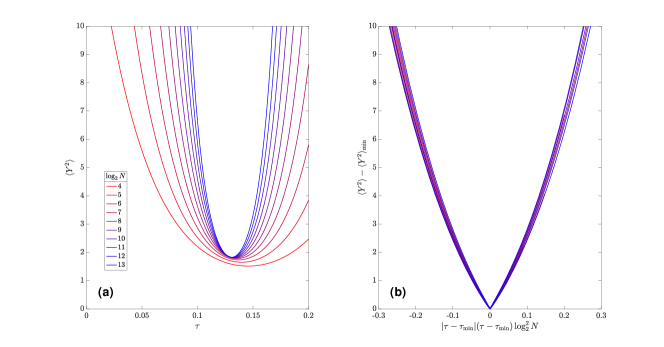
Figure S1: (a) TAT dynamics $S_{\tau}$ evolves initial state $\ket{\bm{0}}$ in rescaled time $\tau$ to a squeezed state with small $\left\langle\Delta Y\right\rangle^{2}=\left\langle Y^{2}\right\rangle$ (since $\left\langle Y\right\rangle=0$), which achieves minimum at $\tau=\tau_{\rm min}\approx 1/8$. Here $\tau_{\rm min}$ is numerically determined for each $N$ (each color). The collapse of curves at $\tau\approx 1/8$ indicates the squeezing is extreme $\Delta Y=\Theta(1)$ at that point. (b) The same data but with axes rescaled, where $\left\langle Y^{2}\right\rangle_{\rm min}$ is the value of $\left\langle Y^{2}\right\rangle$ at $\tau_{\rm min}$. The collapse of curves shows that close to the extreme point, $\left\langle\Delta Y\right\rangle=\Theta(\log N)$ for any nonvanishing $\tau-\tau_{\rm min}$. This leads to an extra $\log N$ factor in the controlled-rotation angle $\phi$.

Figure S2: (a) For fixed $N,\theta$ in the figure title, the encoding infidelity is small in a very narrow window of $\tau_{2}$, which almost does not depend on $\tau_{1}$. (b) The optimal $\tau_{2}$ as a function of $N,\theta$, where $\tau_{1}$ is chosen at $\tau_{1}(\theta,N)$: the $\tau_{1}$ value of the optimal pixel in plots like (a). The collapse of curves on the slope-$1$ line verifies prediction Eq. (15) in the main text for $\tau_{2}$ with constant $c=2$. (c) The optimized $\tau_{3}$ values for the duration of the last unsqueezing stage $S_{\tau_{3}}$, which minimizes the infidelity $\epsilon$ for each set of $(N,\theta,\tau_{1},\tau_{2})$. Here $\tau_{1},\tau_{2}$ are chosen as the optimal ones for each $(N,\theta)$.

References

- Shor (1999) Peter W. Shor, “Polynomial-time algorithms for prime factorization and discrete logarithms on a quantum computer,” SIAM Review 41, 303–332 (1999).
- Harrow et al. (2009) Aram W. Harrow, Avinatan Hassidim, and Seth Lloyd, “Quantum algorithm for linear systems of equations,” Phys. Rev. Lett. 103, 150502 (2009).
- Giovannetti et al. (2004) Vittorio Giovannetti, Seth Lloyd, and Lorenzo Maccone, “Quantum-enhanced measurements: Beating the standard quantum limit,” Science 306, 1330–1336 (2004).
- Greenberger et al. (1989) Daniel M Greenberger, Michael A Horne, and Anton Zeilinger, “Going beyond Bell’s theorem,” in Bell’s theorem, quantum theory and conceptions of the universe, edited by M. Kafatos (Springer, 1989) pp. 69–72.
- Kitagawa and Ueda (1993) Masahiro Kitagawa and Masahito Ueda, “Squeezed spin states,” Phys. Rev. A 47, 5138–5143 (1993).
- Ma et al. (2011) Jian Ma, Xiaoguang Wang, C.P. Sun, and Franco Nori, “Quantum spin squeezing,” Physics Reports 509, 89–165 (2011).
- Bornet et al. (2023) Guillaume Bornet et al., “Scalable spin squeezing in a dipolar Rydberg atom array,” Nature 621, 728–733 (2023), arXiv:2303.08053 [quant-ph] .
- Eckner et al. (2023) William J. Eckner, Nelson Darkwah Oppong, Alec Cao, Aaron W. Young, William R. Milner, John M. Robinson, Jun Ye, and Adam M. Kaufman, “Realizing spin squeezing with Rydberg interactions in an optical clock,” Nature 621, 734–739 (2023), arXiv:2303.08078 [quant-ph] .
- Franke et al. (2023) Johannes Franke, Sean R. Muleady, Raphael Kaubruegger, Florian Kranzl, Rainer Blatt, Ana Maria Rey, Manoj K. Joshi, and Christian F. Roos, “Quantum-enhanced sensing on optical transitions through finite-range interactions,” Nature 621, 740–745 (2023), arXiv:2303.10688 [quant-ph] .
- Korbicz et al. (2005) J. K. Korbicz, J. I. Cirac, and M. Lewenstein, “Spin squeezing inequalities and entanglement of qubit states,” Phys. Rev. Lett. 95, 120502 (2005).
- Korbicz et al. (2006) J. K. Korbicz, O. Gühne, M. Lewenstein, H. Häffner, C. F. Roos, and R. Blatt, “Generalized spin-squeezing inequalities in -qubit systems: Theory and experiment,” Phys. Rev. A 74, 052319 (2006).
- Browaeys and Lahaye (2020) Antoine Browaeys and Thierry Lahaye, “Many-body physics with individually controlled rydberg atoms,” Nature Physics 16, 132–142 (2020).
- Note (1) Here is normalized, and () are Pauli matrices on qubit ; we will also use notations .
- Li et al. (2023) Zeyang Li, null, Simone Colombo, Chi Shu, Gustavo Velez, Saúl Pilatowsky-Cameo, Roman Schmied, Soonwon Choi, Mikhail Lukin, Edwin Pedrozo-Peñafiel, and Vladan Vuletić, “Improving metrology with quantum scrambling,” Science 380, 1381–1384 (2023).
- Cooper et al. (2024) Eric S Cooper, Philipp Kunkel, Avikar Periwal, and Monika Schleier-Smith, “Graph states of atomic ensembles engineered by photon-mediated entanglement,” Nature Physics , 1–6 (2024).
- Britton et al. (2012) Joseph W. Britton, Brian C. Sawyer, Adam C. Keith, C.-C. Joseph Wang, James K. Freericks, Hermann Uys, Michael J. Biercuk, and John J. Bollinger, “Engineered two-dimensional Ising interactions in a trapped-ion quantum simulator with hundreds of spins,” Nature 484, 489–492 (2012).
- Monroe et al. (2021) C. Monroe, W. C. Campbell, L.-M. Duan, Z.-X. Gong, A. V. Gorshkov, P. W. Hess, R. Islam, K. Kim, N. M. Linke, G. Pagano, P. Richerme, C. Senko, and N. Y. Yao, “Programmable quantum simulations of spin systems with trapped ions,” Rev. Mod. Phys. 93, 025001 (2021).
- Pita-Vidal et al. (2024) Marta Pita-Vidal, Jaap J. Wesdorp, and Christian Kraglund Andersen, “Blueprint for all-to-all connected superconducting spin qubits,” (2024), arXiv:2405.09988 [quant-ph] .
- Tran et al. (2020) Minh C. Tran, Chi-Fang Chen, Adam Ehrenberg, Andrew Y. Guo, Abhinav Deshpande, Yifan Hong, Zhe-Xuan Gong, Alexey V. Gorshkov, and Andrew Lucas, “Hierarchy of linear light cones with long-range interactions,” Phys. Rev. X 10, 031009 (2020).
- Tran et al. (2021a) Minh C. Tran, Andrew Y. Guo, Abhinav Deshpande, Andrew Lucas, and Alexey V. Gorshkov, “Optimal state transfer and entanglement generation in power-law interacting systems,” Phys. Rev. X 11, 031016 (2021a).
- Hong and Lucas (2021) Yifan Hong and Andrew Lucas, “Fast high-fidelity multiqubit state transfer with long-range interactions,” Phys. Rev. A 103, 042425 (2021).
- Chen and Lucas (2019) Chi-Fang Chen and Andrew Lucas, “Finite speed of quantum scrambling with long range interactions,” Phys. Rev. Lett. 123, 250605 (2019).
- Kuwahara and Saito (2020) Tomotaka Kuwahara and Keiji Saito, “Strictly linear light cones in long-range interacting systems of arbitrary dimensions,” Phys. Rev. X 10, 031010 (2020).
- Tran et al. (2021b) Minh C. Tran, Andrew Y. Guo, Christopher L. Baldwin, Adam Ehrenberg, Alexey V. Gorshkov, and Andrew Lucas, “Lieb-robinson light cone for power-law interactions,” Phys. Rev. Lett. 127, 160401 (2021b).
- Chen et al. (2023) Chi-Fang (Anthony) Chen, Andrew Lucas, and Chao Yin, “Speed limits and locality in many-body quantum dynamics,” Reports on Progress in Physics 86, 116001 (2023).
- Lucas (2020) Andrew Lucas, “Non-perturbative dynamics of the operator size distribution in the sachdev–ye–kitaev model,” Journal of Mathematical Physics 61, 081901 (2020).
- Yin and Lucas (2020) Chao Yin and Andrew Lucas, “Bound on quantum scrambling with all-to-all interactions,” Phys. Rev. A 102, 022402 (2020).
- Kuwahara and Saito (2021) Tomotaka Kuwahara and Keiji Saito, “Absence of fast scrambling in thermodynamically stable long-range interacting systems,” Phys. Rev. Lett. 126, 030604 (2021).
- Note (2) Throughout, we use big-O notations on the scaling at : () means () for some constant independent of , and means both and . Tildes in e.g. means hiding polylogarithmic factors.
- Note (3) SM also contains symmetry analysis of our protocol, and additional numerical data.
- Note (4) To the best of our knowledge, the only previously-known protocol with a vanishing runtime at large , is a -state Dür et al. (2000) generation protocol Guo et al. (2020), which can be used to perform SWAP gates in short time. Its runtime is still quadratically slower than (5).
- Luo et al. (2024) Chengyi Luo, Haoqing Zhang, Anjun Chu, Chitose Maruko, Ana Maria Rey, and James K. Thompson, “Hamiltonian Engineering of collective XYZ spin models in an optical cavity: From one-axis twisting to two-axis counter twisting models,” (2024), arXiv:2402.19429 [quant-ph] .
- Miller et al. (2024) Calder Miller, Annette N Carroll, Junyu Lin, Henrik Hirzler, Haoyang Gao, Hengyun Zhou, Mikhail D Lukin, and Jun Ye, “Two-axis twisting using Floquet-engineered XYZ spin models with polar molecules,” (2024), arXiv:2404.18913 [cond-mat.quant-gas] .
- Monz et al. (2011) Thomas Monz, Philipp Schindler, Julio T. Barreiro, Michael Chwalla, Daniel Nigg, William A. Coish, Maximilian Harlander, Wolfgang Hänsel, Markus Hennrich, and Rainer Blatt, “14-qubit entanglement: Creation and coherence,” Phys. Rev. Lett. 106, 130506 (2011).
- Pogorelov et al. (2021) I. Pogorelov, T. Feldker, Ch. D. Marciniak, L. Postler, G. Jacob, O. Krieglsteiner, V. Podlesnic, M. Meth, V. Negnevitsky, M. Stadler, B. Höfer, C. Wächter, K. Lakhmanskiy, R. Blatt, P. Schindler, and T. Monz, “Compact ion-trap quantum computing demonstrator,” PRX Quantum 2, 020343 (2021).
- Wang et al. (2018) Xi-Lin Wang, Yi-Han Luo, He-Liang Huang, Ming-Cheng Chen, Zu-En Su, Chang Liu, Chao Chen, Wei Li, Yu-Qiang Fang, Xiao Jiang, Jun Zhang, Li Li, Nai-Le Liu, Chao-Yang Lu, and Jian-Wei Pan, “18-qubit entanglement with six photons’ three degrees of freedom,” Phys. Rev. Lett. 120, 260502 (2018).
- Zhong et al. (2018) Han-Sen Zhong, Yuan Li, Wei Li, Li-Chao Peng, Zu-En Su, Yi Hu, Yu-Ming He, Xing Ding, Weijun Zhang, Hao Li, Lu Zhang, Zhen Wang, Lixing You, Xi-Lin Wang, Xiao Jiang, Li Li, Yu-Ao Chen, Nai-Le Liu, Chao-Yang Lu, and Jian-Wei Pan, “12-photon entanglement and scalable scattershot boson sampling with optimal entangled-photon pairs from parametric down-conversion,” Phys. Rev. Lett. 121, 250505 (2018).
- Song et al. (2019) Chao Song, Kai Xu, Hekang Li, Yu-Ran Zhang, Xu Zhang, Wuxin Liu, Qiujiang Guo, Zhen Wang, Wenhui Ren, Jie Hao, Hui Feng, Heng Fan, Dongning Zheng, Da-Wei Wang, H. Wang, and Shi-Yao Zhu, “Generation of multicomponent atomic schrödinger cat states of up to 20 qubits,” Science 365, 574–577 (2019).
- Mooney et al. (2021) Gary J Mooney, Gregory A L White, Charles D Hill, and Lloyd C L Hollenberg, “Generation and verification of 27-qubit greenberger-horne-zeilinger states in a superconducting quantum computer,” Journal of Physics Communications 5, 095004 (2021).
- Omran et al. (2019) A. Omran, H. Levine, A. Keesling, G. Semeghini, T. T. Wang, S. Ebadi, H. Bernien, A. S. Zibrov, H. Pichler, S. Choi, J. Cui, M. Rossignolo, P. Rembold, S. Montangero, T. Calarco, M. Endres, M. Greiner, V. Vuletić, and M. D. Lukin, “Generation and manipulation of schrödinger cat states in rydberg atom arrays,” Science 365, 570–574 (2019).
- Cao et al. (2024) Alec Cao et al., “Multi-qubit gates and ’Schrödinger cat’ states in an optical clock,” (2024), arXiv:2402.16289 [quant-ph] .
- Ho et al. (2019) Wen Wei Ho, Cheryne Jonay, and Timothy H. Hsieh, “Ultrafast variational simulation of nontrivial quantum states with long-range interactions,” Phys. Rev. A 99, 052332 (2019).
- Alexander et al. (2020) Byron Alexander, John J. Bollinger, and Hermann Uys, “Generating greenberger-horne-zeilinger states with squeezing and postselection,” Phys. Rev. A 101, 062303 (2020).
- Zhao et al. (2021) Yajuan Zhao, Rui Zhang, Wenlan Chen, Xiang-Bin Wang, and Jiazhong Hu, “Creation of Greenberger-Horne-Zeilinger states with thousands of atoms by entanglement amplification,” npj Quantum Inf. 7, 24 (2021).
- Comparin et al. (2022a) Tommaso Comparin, Fabio Mezzacapo, and Tommaso Roscilde, “Multipartite entangled states in dipolar quantum simulators,” Phys. Rev. Lett. 129, 150503 (2022a).
- Wang et al. (2023) Lingxia Wang et al., “Entangling spins using cubic nonlinear dynamics,” (2023), arXiv:2301.04520 [quant-ph] .
- Zhang et al. (2023) Tao Zhang, Zhihao Chi, and Jiazhong Hu, “Entanglement generation via single-qubit rotations in a teared Hilbert space,” (2023), arXiv:2312.04507 [quant-ph] .
- Zhang et al. (2024) Xuanchen Zhang, Zhiyao Hu, and Yong-Chun Liu, “Fast generation of ghz-like states using collective-spin model,” Phys. Rev. Lett. 132, 113402 (2024).
- Yin and Lucas (2024) Chao Yin and Andrew Lucas, “Heisenberg-limited metrology with perturbing interactions,” Quantum 8, 1303 (2024).
- Omanakuttan et al. (2024) Sivaprasad Omanakuttan, Vikas Buchemmavari, Jonathan A. Gross, Ivan H. Deutsch, and Milad Marvian, “Fault-tolerant quantum computation using large spin-cat codes,” PRX Quantum 5, 020355 (2024).
- Shor (1995) Peter W. Shor, “Scheme for reducing decoherence in quantum computer memory,” Phys. Rev. A 52, R2493–R2496 (1995).
- Liu et al. (2011) Y. C. Liu, Z. F. Xu, G. R. Jin, and L. You, “Spin squeezing: Transforming one-axis twisting into two-axis twisting,” Phys. Rev. Lett. 107, 013601 (2011).
- Hosten et al. (2016) O. Hosten, R. Krishnakumar, N. J. Engelsen, and M. A. Kasevich, “Quantum phase magnification,” Science 352, 1552–1555 (2016).
- Note (5) We expect that this naive separation strategy (with the latter stages adjusted accordingly) also yields an approximate GHZ encoding protocol with very small infidelity up to relatively large , similar to what we will show for (7). Although the scaling is suboptimal comparing to (13), it still beats the naive protocol with CNOTs.
- Note (6) Note that the -local squeezing dynamics in Zhang et al. (2024) has the same squeezing directions at the two poles, so in principle can be used here to unsqueeze. However, we do not use that because as mentioned earlier, the -local interaction requires changing the -local Hamiltonian very rapidly to engineer.
- Perlin et al. (2020) Michael A. Perlin, Chunlei Qu, and Ana Maria Rey, “Spin squeezing with short-range spin-exchange interactions,” Phys. Rev. Lett. 125, 223401 (2020).
- Comparin et al. (2022b) Tommaso Comparin, Fabio Mezzacapo, and Tommaso Roscilde, “Robust spin squeezing from the tower of states of u(1)-symmetric spin hamiltonians,” Phys. Rev. A 105, 022625 (2022b).
- Block et al. (2023) Maxwell Block, Bingtian Ye, Brenden Roberts, Sabrina Chern, Weijie Wu, Zilin Wang, Lode Pollet, Emily J. Davis, Bertrand I. Halperin, and Norman Y. Yao, “A Universal Theory of Spin Squeezing,” (2023), arXiv:2301.09636 [quant-ph] .
- Dür et al. (2000) W. Dür, G. Vidal, and J. I. Cirac, “Three qubits can be entangled in two inequivalent ways,” Phys. Rev. A 62, 062314 (2000).
- Guo et al. (2020) Andrew Y. Guo, Minh C. Tran, Andrew M. Childs, Alexey V. Gorshkov, and Zhe-Xuan Gong, “Signaling and scrambling with strongly long-range interactions,” Phys. Rev. A 102, 010401 (2020).