Watermarking Language Models with Error Correcting Codes
Abstract
Recent progress in large language models enables the creation of realistic machine-generated content. Watermarking is a promising approach to distinguish machine-generated text from human text, embedding statistical signals in the output that are ideally undetectable to humans. We propose a watermarking framework that encodes such signals through an error correcting code. Our method, termed robust binary code (RBC) watermark, introduces no distortion compared to the original probability distribution, and no noticeable degradation in quality. We evaluate our watermark on base and instruction fine-tuned models and find our watermark is robust to edits, deletions, and translations. We provide an information-theoretic perspective on watermarking, a powerful statistical test for detection and for generating -values, and theoretical guarantees. Our empirical findings suggest our watermark is fast, powerful, and robust, comparing favorably to the state-of-the-art.
1 Introduction
As language model capabilities improve, there are corresponding potential harms such as the creation of misinformation (Zellers et al., 2020) and propaganda (Solaiman et al., 2019). To mitigate this, a first step is to detect and filter content. A popular approach to reliably detecting AI generated content is to add a watermark (Kirchenbauer et al., 2023; Kuditipudi et al., 2023; Aaronson and Kirchner, 2022; Christ et al., 2023), a hidden signal embedded in the output. While there are exponentially many combinations of words and characters, watermarking biases generation towards specific patterns that are undetectable to humans.
We consider the detection setting from the model-provider’s perspective: the detection algorithm receives (user or machine-generated) text as input, but no further metadata such as prompts or generation parameters. We do not explore zero-shot or post-hoc methods to classify text as generated from any language model, such as GPT-Zero (Tian and Cui, 2023) and DetectGPT (Mitchell et al., 2023). This model-agnostic detection is inherently challenging as language models are trained to mimic human text (Bender et al., 2021). as language models become more powerful, their generation becomes nearly indistinguishable from human-generated text, thereby reducing the efficacy of zero-shot classification methods. Instead, we explore how to introduce statistical signals into the generation process to reliably classify text as watermarked.
Desiderata. We focus on the following list of practical, empirical and algorithmic desiderata (and some others) for an effective watermark, inspired by, e.g., (Kuditipudi et al., 2023; Kirchenbauer et al., 2023; Piet et al., 2023).
-
•
Robust: The watermark should be robust to watermarking attacks and perturbations, such as edits and deletions of significant fractions of the text, translation attacks, paraphrasing, etc.
-
•
Quality-Preserving: The watermark should not decrease the quality of the outputs of the language model. This can be achieved by making the watermark distortion-free, i.e., by preserving the distribution of the original language model.
-
•
Model Agnostic: The watermark should apply to any language model. This is important to be applicable to future models.
-
•
High Detection Power: The watermark should be detectable with only a small number of tokens.
Prior watermarking schemes achieve many but not all of these qualities. For instance, Kuditipudi et al. (2023) introduces distortion-free watermarks that do not modify the output distribution in expectation (but their detection power is limited due to using permutation tests). Taking a cryptographic perspective, Christ et al. (2023) introduces theoretically undetectable watermarks (but does not illustrate their performance empirically). We obtain highly powerful watermarks without sacrificing generation quality. Qu et al. (2024) develop a provably robust watermark via error correction codes, focusing on embedding a multi-bit string (such as an user ID) in the text. Our focus (e.g., distortion-freeness), our methods (binarization, correlated binary channel, LDPC codes) , and our theoretical guarantees (high detection probability), are different. For further discussions on prior and related work, see Appendix A.
Contributions. We propose the Robust Binary Code (RBC) watermark using error correcting codes, and argue the following claims:
-
•
Robustness. RBC achieves several forms of robustness (e.g., to user edits) by leveraging error correcting codes.
-
•
Power and Quality. Our RBC watermark is distortion-free, thus keeping the quality of the original language model unchanged. Further, RBC empirically leads to strongly detectable watermarks, competitive with state-of-the-art watermarks that introduce distortion.
-
•
Simplicity. Our RBC watermark is simple to use, as it wraps around the output logits of the language model.
2 Background
2.1 Error Correcting Codes
To introduce our method, we need to provide some background on error correcting codes. For a positive integer , we use the Hamming distance on , such that for , is the number of differing coordinates of . We recall some standard definitions (MacWilliams and Sloane, 1977; Huffman and Pless, 2010).
Definition 2.1.
For positive integers , an error correcting code (ECC) is an injective map . The message space is . Applying to a message is known as encoding, and is known as a codeword. The rate of the code is .
The error correcting distance of is the greatest such that for all messages , there exists at most one codeword in the Hamming ball of radius of around , . Such a code is known as a -code.
Given a -error correcting code , we may define a decoding map . For a given , the decoding is the unique such that , if such a exists; and otherwise, the decoding is defined arbitrarily. By definition, at most one such exists.
2.2 Notation
We use the following notation throughout this work. We typically use capital letters to denote random variables. For a positive integer and , let be the CDF of a random variable at the positive integer , and let . Let be the vocabulary of the language model, with commonly between 50,000 to 200,000 in our current applications, and let be the set of strings of tokens from of arbitrary length. For a positive integer , we use to denote the tokens generated by the language model , and write for any sequence of previous tokens. Let be the distribution of the next tokens. For some positive integers , Let be a error correcting code.
2.3 Reduction to Binary Vocabulary
Motivated by Christ et al. (2023), we reduce language modeling to a minimal binary vocabulary. To do so, we assign to each token a unique bit string. For a vocabulary of size , this requires total bits; typically between and bits in our current applications. We use an injective binary encoder that maps tokens to bit strings. A single token sampled from the language model induces a distribution over the next bits, determined by the encoder . We use to denote the probability of the next bit being one () given previous bits . We will write from now on.
In our watermarking scheme, we use the following variables: is the message passed through the error correcting code to obtain the codeword . The binary sampling scheme generates bits that are correlated with the ’s (as explained in Section 3). We use the previous tokens to modify the distribution of the following tokens. Each application of our watermarking scheme generates a block of tokens, using the previous tokens.
3 Key Watermarking Tool
For our watermarking scheme, we systematically encode signals into generated tokens. However, doing so by biasing the logits as in Kirchenbauer et al. (2023) perturbs the distribution of tokens, resulting in distorted generation. Instead, we propose a distortion-free generation technique to encode signals. As described before, to introduce this technique, we first reduce from an arbitrary vocabulary to a binary vocabulary, where the language model generates bits. Recall that .
Given a message that we wish to transmit, we generate a codeword . We next explain how to embed this codeword without inducing distortion.
3.1 Correlated Binary Sampling Channel (CBSC)
To introduce our method, we first take a step back and consider the setting of sampling Bernoulli random variables. An equivalent way to sample , is to introduce an auxiliary random variable and let . Notably, and are now correlated.
A further equivalent sampling scheme is to let , where and are sampled independently; so that . By writing in binary, represents the most significant bit of , and represents the remaining bits. Therefore, we have the following sampling scheme for :
| (1) | ||||
We call this sampling process the Correlated Binary Sampling Channel (CBSC), where we use an auxiliary random variable to sample a biased (non-uniform) bit , ensuring are correlated. We use rather than simply so that and are positively correlated; but the methods are equivalent. This CBSC is equivalent to the binary generation scheme from the recent work Christ and Gunn (2024), although with a different formulation and motivation.
Distortion-freeness. Crucially, the CBSC ensures that matches its target distribution despite using the external information , i.e., . Thus, the CBSC is a distortion-free method.
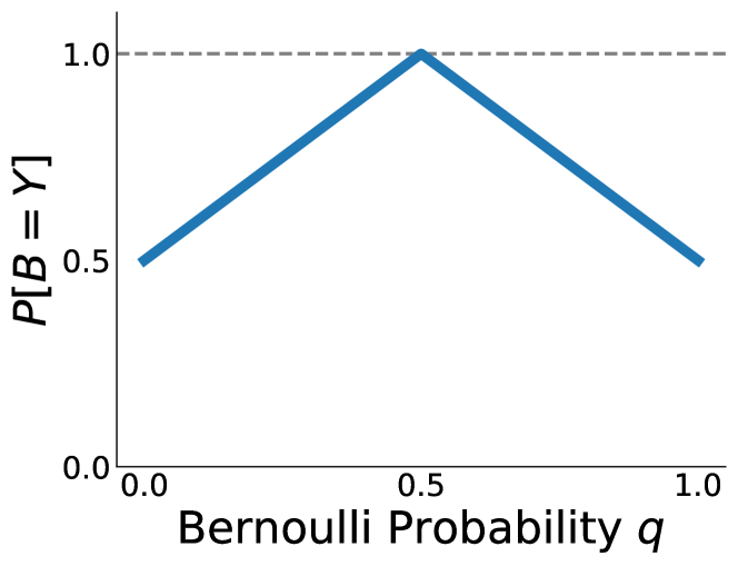
We plot the transition probabilities between and in Figure 1(a). We also show the matching probability between and as a function of the probability in Figure 1(b). When the entropy of is maximized, i.e., when , then we deterministically have . However, when —so has zero entropy—then and contains no information about . In general, the sampled bit is biased towards and is more likely to be equal to than not.
3.2 Simple Watermark
The CBSC in Equation 1 is our key mechanism for watermarking, enabling distortion-free sampling with detectable correlation. We embed a sequence of known bits into our generated bits . Generating bits through the CBSC ensures follows the original probability distribution–i.e., is distortion-free—and yet biases towards .
We may use this statistical dependence to detect whether or not the text was watermarked. For unwatermarked text, and are uncorrelated and therefore , whereas for watermarked text, we expect . This is the basis of our simple one-to-one watermarking scheme, described in Section B.4. We will later improve this by reducing errors in our binary channel by leveraging error correcting codes.
Choosing known bits . In order to reliably detect the watermark, we need to know the bits used in the CBSC. One approach is to use a long fixed bit string, a secret sequence known to the language model provider. Kuditipudi et al. (2023) use a similar approach with a fixed list of real numbers and use the edit distance to capture correlations. However, this approach is sensitive to the relative indexing of the text, and the fixed list and can be susceptible to attacks that shuffle the text. Instead, we use a sliding window of previously generated tokens to serve as sources of randomness for . This sliding window approach is popular in watermarking schemes, see e.g., Aaronson and Kirchner (2022); Kirchenbauer et al. (2023); Christ et al. (2023). We thus use text-dependent randomness (Piet et al., 2023) to generate pseudorandom bits , leveraging previous tokens to obtain pseudorandom outputs.
Error correcting codes in generation. The purpose of using error correcting codes (ECCs) is to reduce mismatches between and . Rather than directly transmitting , we add redundancy through a ECC . We choose a shorter message and use . When using an ECC, we choose by hashing the previous bits, and then apply the error correcting code to to obtain our codeword . By using , we can correct errors in the CBSC. Specifically, if , then , giving a strong indication that the text was in fact watermarked.
Combining these parts, our watermarking scheme contains the following steps:
-
1.
Create message: Use previous tokens to create message .
-
2.
Encode using : Encode using ECC to obtain .
-
3.
Generate: Transmit using CBSC with probabilities from the language model to generate .
-
4.
Repeat: Perform the above steps until the stopping condition.
We call each sequence of bits generated at an iteration a block. In Algorithm 1 and Algorithm 2, we present a simplified watermark and detection algorithm that captures the essence of our approach.
4 Robust Binary Code Watermark
Next, we present our robust binary code (RBC) watermark, which converts tokens to binary, applies an error correcting code for robustness, and generates bits through the CBSC.
Let be the number of bits for each token and let and . Assume we have an injective binary encoder which maps from tokens to bit strings, and the corresponding binary decoder (defined arbitrarily for strings outside of the image of ). We also have the language model induced by over a binary alphabet, so that for any binary string . We let the encoder operate on a list of tokens elementwise, and the decoder operate on blocks of bits of length .
Our full watermarking scheme is shown in Algorithms 3, 4, 5 and 6. Algorithms 3 and 4 expand on the simplified method from Algorithm 1, and Algorithms 5 and 6 expand on the detection in Algorithm 2. The RBC watermark is very similar to the simplified watermark in Section 3.2, with the addition of the binary encoder/decoder . In the generation of the messages , we also apply an exclusive or between the previous bits with a randomly chosen bitstring to ensure the message contains i.i.d. entries. In this step, we could also apply the minimum hashing method from Kirchenbauer et al. (2023).
5 Theoretical Results
We now provide theoretical guarantees for our methods, focusing on how the entropy of the language model affects watermarking. For the following results, we consider a language model with a binary vocabulary that generates bits . Let for any positive integer and bit string . We provide the proofs of all of the following claims in Appendix D. We start with some preliminaries.
Definition 5.1 (Entropy).
Let the entropy of a Bernoulli random variable with success probability be defined as , with . For a sequence of (possibly dependent) Bernoulli random variables with respective success probabilities , let the average entropy be .
We will need the following lemma, which bounds the entropy in terms of , .
Lemma 5.2.
For , we have the inequality . For , we have the inequality
| (2) |
We plot the bounds on the entropy for the single-variate case in Figure 2. Next, using the above result, we turn to analyzing the CBSC. With for all and , let the average entropy of the language model be . Intuitively, we expect that watermarking should be easier when the entropy is large (), as there are more methods to embed signals and keep the distribution unchanged. The next result supports this intuition.

Theorem 5.3 (Bounding the proportion of mismatches in a CSBC with the entropy).
The expected proportion of mismatches between the generated and codeword —i.e., —is bounded by
This theorem bounds the error probability in terms of the average entropy of the language model, showing that the frequency of errors is both upper and lower bounded by a monotone decreasing function of . In particular as . This is consistent with watermarking being easier when the entropy is high.
The above result shows that the mean of is upper bounded by . Therefore, it is reasonable to assume that for some and a small , with probability at least . Our next result will be presented under this condition.
Theorem 5.4 (Exact block decoding).
Consider a language model such that for . Let the average entropy of the language model be . Suppose that for some , with probability at least . Assume is an error correcting code where . Then for a codeword , the generated bits from Algorithm 4 satisfy
The above theorem bounds the probability that a specific block exactly decodes to the codeword . In particular, it gives a bound where the decoding block probability decreases as the entropy of the language model decreases. In particular if and is small, the decoding happens with high probability. This is consistent with the fact that watermarking is more difficult for models with less entropy when is small, in which case needs to be large.
6 Experimental Results
We evaluate the performance of RBC in a suite of experiments to measure watermarking detectability and robustness to state-of-the-art watermarking schemes.
6.1 Watermark Detection
Generation procedure. We use three prompts inspired by Piet et al. (2023), involving writing a 1) book report, 2) story, and 3) fake news article. Piet et al. (2023) used these text generation tasks to represent realistic settings with long-form generated text, where the model provider may like to watermark the outputs. We provide the full prompts used for generation in Appendix E.
We generate responses for each prompt for five lengths ranging from 10 to 150 tokens, representing a few sentences to a few paragraphs. We use the Llama-3-8B base model AI@Meta (2024), a powerful open-source model capable of high quality generation.
Baselines and hyperparameters. We compare the performance of RBC to the watermarking algorithm from Kirchenbauer et al. (2023), which we denote as the Distribution Shift method. The thorough evaluation from Piet et al. (2023) finds this to be the most effective and powerful watermark, and concludes that it serves as the current state-of-the-art.
In practice, many ECCs with varying guarantees exist, including Bose and Ray-Chaudhuri (1960); Gallager (1962); Reed and Solomon (1960). Different ECCs provide different guarantees, e.g., robustness to bit flips or edit distance. For this work, we explore two ECCs. We primarily use the popular low-density parity-check (LDPC) code (Gallager, 1962) for our watermarking scheme. As a baseline, we also use a custom code which we call a one-to-one code. Our one-to-one code has and is equivalent to the identity function, i.e., the one-to-one codes do not provide error correcting capabilities. We use this as a baseline to compare the impact of the error correcting functionality. For more details on our one-to-one code, see Section B.4. We use the LDPC code (Shokrollahi, 2004) with
, , , , and a one-to-one code with , using and , and set to be a random binary enumeration.
For the distribution shift method from Kirchenbauer et al. (2023), we use their suggested hyperparameters. A key parameter is , the level of distribution shift induced by the watermarking procedure. Greater values of result in larger distribution shifts and more detectable watermarking. The authors recommend for watermarking. In our experiments, we choose to use and to represent medium and strong distribution shifts.
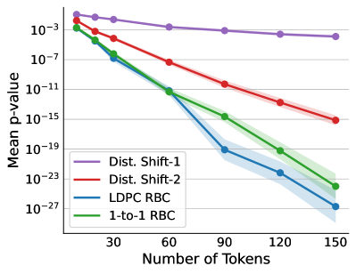
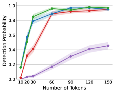
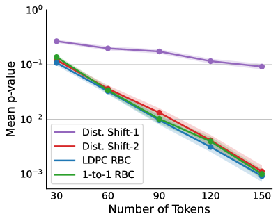
Evaluation. For each generation, we use the -value of the detection procedure on the output text. We compute the mean of the log--values (instead of the -values themselves) for each generation to more accurately capture the signal strength. We also report the detection probability or power—the percentage of generations with -values less than —to represent how likely the text is to be classified as watermarked.
From the summary statistics in Table 1 and Figure 3, we observe that our RBC watermarking method shows substantial improvements in detectability compared to the distribution shift scheme (Kirchenbauer et al., 2023) with and , with p-values smaller by many orders of magnitude. Further, RBC improves performance by using the LDPC code compared to the one-to-one code, suggesting improvements by using an ECC. We observe consistent detectability with as few as 20-30 tokens. This suggests that the RBC watermark outperforms the current state-of-the-art distribution shift watermark from Kirchenbauer et al. (2023) here, requiring approximately half as many tokens for equivalent detectability.
| 20 Tokens | 150 Tokens | |||||
|---|---|---|---|---|---|---|
| Method | Mean | Median | Detect % | Mean | Median | Detect % |
| LDPC RBC | % | % | ||||
| One-to-one RBC | % | % | ||||
| Dist. Shift | % | % | ||||
| Dist. Shift | % | % | ||||
6.2 Robustness Experiments
In practice, a user may attempt to circumvent watermarks by editing the text generated by a language model. To emulate this, we use three popular perturbations that may represent an adversary hoping to evade a watermark, as in other works including (Kuditipudi et al., 2023; Piet et al., 2023).
-
1.
Delete. We randomly delete of the tokens.
-
2.
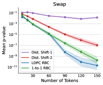
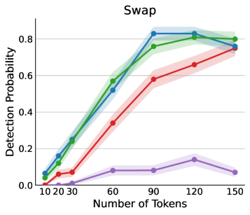
Swap. We replace a randomly chosen fraction of of the tokens with random tokens.
-
3.
Translate. We translate the generated text to Russian then back to English using Argos Translate (Finlay and Argos Translate, 2023).
For our experiments, we elect to perturb of the tokens, as this represents a relatively high noise regime where one in five tokens are modified. In our translation perturbation, we choose to translate to Russian and then back to English for a powerful attack, as Russian and English are relatively different compared to Spanish and French, see e.g., Anttila (1972), etc.
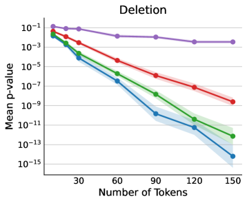
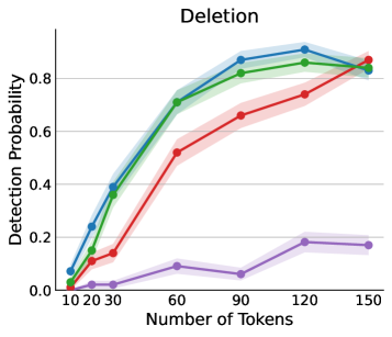
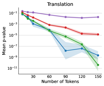
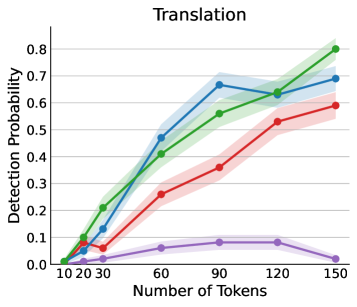
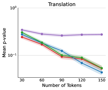
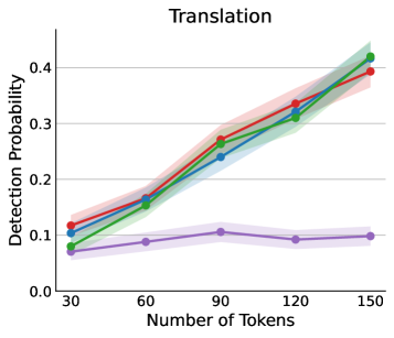
In Table 3 and Figure 6, we evaluate the robustness of RBC and the distribution shift watermarking scheme to the perturbations. Notably, the LDPC and one-to-one RBC watermarks show the greatest robustness. They achieve consistent detectability with 60 tokens. For further plots, see Section C.1.
| 20 Tokens | 150 Tokens | ||||||
|---|---|---|---|---|---|---|---|
| Method | Mean | Median | Detect % | Mean | Median | Detect % | |
| Swap | LDPC RBC | % | % | ||||
| One-to-one RBC | % | % | |||||
| Dist. Shift | % | % | |||||
| Dist. Shift | % | % | |||||
| Delete | LDPC RBC | % | % | ||||
| One-to-one RBC | % | % | |||||
| Dist. Shift | % | % | |||||
| Dist. Shift | % | % | |||||
| Translate | LDPC RBC | % | % | ||||
| One-to-one RBC | % | % | |||||
| Dist. Shift | % | % | |||||
| Dist. Shift | % | % | |||||
6.3 Instruction Fine-tuned Models
We conduct ablation experiments on the dependence of the language model. Instead of the base Llama-3-8B model, we consider the instruction fine-tuned model, optimized to answer queries. It is well known—see e.g., Piet et al. (2023)—that instruction fine-tuned models tend to be more certain of the next-token predictions, and therefore have less entropy and are more difficult to watermark. We use the same generation and hyperparameters as Section 6.1 but with the Llama-3-8B base model, and we use an LDPC code with , , , , and a one-to-one code with for this lower entropy regime. We plot the mean log p-values in the left plot of Figure 4.
Compared to the base fine-tuned model, the instruction fine-tuned model has substantially lower entropy, and it is more difficult to add consistent statistical signals. For the distribution shift watermark with , we see poor detectability and large p-values. The RBC watermark exhibits similar performance to the distribution shift watermark with , with minor improvements from the LDPC code. This shows that RBC has watermarking detection power competitive with the state-of-the-art method Kirchenbauer et al. (2023) without inducing distortion. For further details and robustness experiments on the instruct model, see Section C.2.
6.4 Generation Quality
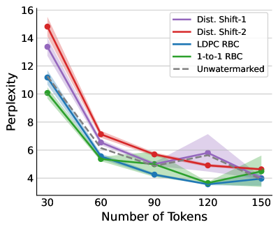
A key aspect of watermarking is ensuring the quality of the generated outputs remains constant. As a simple test, we evaluate the perplexity of the generated text using the various watermarking schemes and compare it against the baseline of unwatermarked text in the right plot of Figure 4. We use Llama-3-8B-Instruct for the perplexity computations.
We observe the distribution shift watermark increases the perplexity of the outputs, with greater increases from greater choices of . This suggests that the addition of distortion may result in mild degradation in quality. In contrast, the RBC watermarks result in minimal changes to the perplexity. This suggests that RBC does not noticeably lower text quality, but this may happen for distortion-inducing watermarks.
7 Conclusion
We propose the new RBC watermarking scheme, using error correcting codes to reliably embed a statistical signal in the text generated from a language model. The RBC watermark empirically has high detection power and is robust to perturbations, while retaining the quality of the generated text. The watermark is applicable to any language model, as it only requires the probability distribution of tokens as input.
We find the RBC watermark outperforms the current state-of-the-art distribution shift watermark from Kirchenbauer et al. (2023) on the powerful base model Llama-3-8B AI@Meta (2024). On the instruction fine-tuned model, we attain comparable performance without any distortion or noticeable degradation in quality. Furthermore, the RBC watermark is empirically robust to edits and translation attacks.
7.1 Limitations and Broader Impact
While our preliminary experiments are promising, we plan to evaluate broader classes of perturbations, generation tasks, and language models for more comprehensive experimentation. Additionally, there are many choices of ECCs to choose from, e.g., BCH, LDPC, Turbo codes, etc., with corresponding code parameters. We hope to evaluate the effect of the choice of an ECC in future work.
As AI-generated content becomes more prolific, there are incentives for both users and providers to watermark this content. Users would like to determine whether content was human- or AI-generated with high certainty, and language model providers are motivated to add these watermarks without sacrificing quality. With additional future work, it would be a highly desirable outcome if a watermark such as RBC could effectively balance both incentives.
Acknowledgements
Patrick Chao and Edgar Dobriban were supported in part by the ARO, ONR, the NSF, and the Sloan Foundation. Any opinions, findings and conclusions or recommendations expressed in this material are those of the authors and do not necessarily reflect the views of the Army Research Office (ARO), or the Department of Defense, or the United States Government. The authors would like to thank Alex Li, Daniel Geng, and Surbhi Goel for the support and feedback.
References
- Aaronson and Kirchner (2022) S. Aaronson and H. Kirchner. Watermarking gpt outputs, 2022. URL https://www.scottaaronson.com/talks/watermark.ppt.
- AI@Meta (2024) AI@Meta. Llama 3 model card, 2024. URL https://github.com/meta-llama/llama3/blob/main/MODEL_CARD.md.
- Anttila (1972) R. Anttila. An introduction to historical and comparative linguistics. Macmillan New York, 1972.
- Atallah et al. (2001) M. J. Atallah, V. Raskin, M. Crogan, C. F. Hempelmann, F. Kerschbaum, D. Mohamed, and S. Naik. Natural language watermarking: Design, analysis, and a proof-of-concept implementation. In Information Hiding, 2001. URL https://api.semanticscholar.org/CorpusID:37687669.
- Bender et al. (2021) E. M. Bender, T. Gebru, A. McMillan-Major, and S. Shmitchell. On the dangers of stochastic parrots: Can language models be too big? In Proceedings of the 2021 ACM Conference on Fairness, Accountability, and Transparency, FAccT ’21, page 610–623, New York, NY, USA, 2021. Association for Computing Machinery. ISBN 9781450383097. doi: 10.1145/3442188.3445922. URL https://doi.org/10.1145/3442188.3445922.
- Bose and Ray-Chaudhuri (1960) R. Bose and D. Ray-Chaudhuri. On a class of error correcting binary group codes. Information and Control, 3(1):68–79, 1960. ISSN 0019-9958. doi: https://doi.org/10.1016/S0019-9958(60)90287-4. URL https://www.sciencedirect.com/science/article/pii/S0019995860902874.
- Christ and Gunn (2024) M. Christ and S. Gunn. Pseudorandom error-correcting codes, 2024.
- Christ et al. (2023) M. Christ, S. Gunn, and O. Zamir. Undetectable watermarks for language models. URL https://eprint. iacr. org/2023/763, 2023.
- Finlay and Argos Translate (2023) P. Finlay and C. Argos Translate. Argos Translate, 2023. URL https://github.com/argosopentech/argos-translate.
- Gallager (1962) R. Gallager. Low-density parity-check codes. IRE Transactions on Information Theory, 8(1):21–28, 1962. doi: 10.1109/TIT.1962.1057683.
- Huffman and Pless (2010) W. C. Huffman and V. Pless. Fundamentals of error-correcting codes. Cambridge University Press, 2010.
- Katzenbeisser and Petitcolas (1999) S. Katzenbeisser and F. Petitcolas. Information hiding techniques for steganography and digital watermaking. Edpacs, 28:1–2, 12 1999. doi: 10.1201/1079/43263.28.6.20001201/30373.5.
- Kirchenbauer et al. (2023) J. Kirchenbauer, J. Geiping, Y. Wen, J. Katz, I. Miers, and T. Goldstein. A watermark for large language models, 2023.
- Kuditipudi et al. (2023) R. Kuditipudi, J. Thickstun, T. Hashimoto, and P. Liang. Robust distortion-free watermarks for language models, 2023.
- MacWilliams and Sloane (1977) F. J. MacWilliams and N. J. A. Sloane. The theory of error-correcting codes. Elsevier, 1977.
- Mitchell et al. (2023) E. Mitchell, Y. Lee, A. Khazatsky, C. D. Manning, and C. Finn. Detectgpt: Zero-shot machine-generated text detection using probability curvature, 2023. URL https://arxiv.org/abs/2301.11305.
- Piet et al. (2023) J. Piet, C. Sitawarin, V. Fang, N. Mu, and D. Wagner. Mark my words: Analyzing and evaluating language model watermarks, 2023.
- Qu et al. (2024) W. Qu, D. Yin, Z. He, W. Zou, T. Tao, J. Jia, and J. Zhang. Provably robust multi-bit watermarking for ai-generated text via error correction code. arXiv preprint arXiv:2401.16820, 2024.
- Reed and Solomon (1960) I. S. Reed and G. Solomon. Polynomial codes over certain finite fields. Journal of the Society for Industrial and Applied Mathematics, 8(2):300–304, 1960. doi: 10.1137/0108018. URL https://doi.org/10.1137/0108018.
- Shokrollahi (2004) A. Shokrollahi. Ldpc codes: An introduction. In Coding, cryptography and combinatorics, pages 85–110. Springer, 2004.
- Solaiman et al. (2019) I. Solaiman, M. Brundage, J. Clark, A. Askell, A. Herbert-Voss, J. Wu, A. Radford, G. Krueger, J. W. Kim, S. Kreps, M. McCain, A. Newhouse, J. Blazakis, K. McGuffie, and J. Wang. Release strategies and the social impacts of language models, 2019.
- Tian and Cui (2023) E. Tian and A. Cui. Gptzero: Towards detection of ai-generated text using zero-shot and supervised methods”, 2023. URL https://gptzero.me.
- Wilks (1938) S. S. Wilks. The Large-Sample Distribution of the Likelihood Ratio for Testing Composite Hypotheses. The Annals of Mathematical Statistics, 9(1):60 – 62, 1938. doi: 10.1214/aoms/1177732360. URL https://doi.org/10.1214/aoms/1177732360.
- Zellers et al. (2020) R. Zellers, A. Holtzman, H. Rashkin, Y. Bisk, A. Farhadi, F. Roesner, and Y. Choi. Defending against neural fake news, 2020.
Appendix A Further Related Work
Watermarking text is closely related to steganography, and has been of interest for many years (Katzenbeisser and Petitcolas, 1999; Atallah et al., 2001). In modern watermarking, Aaronson and Kirchner (2022), in collaboration with OpenAI, propose a biasing-based watermarking method utilizing exponential minimum sampling by hashing previous tokens. Kirchenbauer et al. (2023) explores introducing biases in the logits by splitting the set of tokens into red and green sets also by hashing previous tokens. By biasing the logits for tokens in the green set, this adds a mild distortion and recoverable signal.
Kuditipudi et al. (2023) introduces the notion of distortion-free watermarks. Rather than introducing systematic biases in the logits from the language model, distortion-free watermarks preserve the distribution of logits in expectation. Furthermore, the proposed distortion-free watermark enjoys edit-distance robustness guarantees. However, since this work uses permutation tests, it can be expensive to obtain small -values required for high power.
Christ et al. (2023) furthers this distortion-free generation to undetectable watermarks—watermarks that can only be detected with negligible probability with a polynomial number of queries. However, since this work does not provide an empirical implementation and experiments, the practical performance and implementation difficulties of remain unexplored.
In the concurrent work (Christ and Gunn, 2024), the authors introduce pseudorandom codes (PRC) for watermarking. They use an analogous generation scheme to the CBSC, using the encoded message from the PRC to generate watermarked bits. In contrast with RBC, we primarily focus on the implementation and practical application of watermarking, providing explicit implementations and experimental results, whereas their work provides detailed theoretical discussions but no empirical implementation details or evaluations.
Appendix B Implementation Details
B.1 Compute Details
All experiments were run on two Nvidia 3090 GPUs, for a total of 24 GPU hours. Each prompt of 500 generations with three perturbations takes approximately two GPU hours.
B.2 Detection Algorithms
B.3 Alternative Statistical Tests
We also explore alternative statistical tests to the simple binary comparison test in Algorithm 6. These use the generalized likelihood ratio test, and use Wilks’s theorem (Wilks, 1938) to approximate the distribution of the log-likelihood ratio by a distribution.
B.4 One-to-one Code
Our one-to-one code is very simple: maps between length bit strings, and is defined as , where is a fixed bit string. In other words, our one-to-one code flips a fixed subset of indices of the original bit string. We choose with i.i.d. entries, so that also contains random entries.
Appendix C Additional Experimental Results
C.1 Llama-3-8B Base Watermarking
C.2 Llama-3-8B-Instruct Robustness
| 30 Tokens | 150 Tokens | ||||||
|---|---|---|---|---|---|---|---|
| Method | Mean | Median | Detect % | Mean | Median | Detect % | |
| No Pert. | LDPC RBC | % | % | ||||
| One-to-one RBC | % | % | |||||
| Dist. Shift | % | % | |||||
| Dist. Shift | % | % | |||||
| Swap | LDPC RBC | % | % | ||||
| One-to-one RBC | % | % | |||||
| Dist. Shift | % | % | |||||
| Dist. Shift | % | % | |||||
| Delete | LDPC RBC | % | % | ||||
| One-to-one RBC | % | % | |||||
| Dist. Shift | % | % | |||||
| Dist. Shift | % | % | |||||
| Translate | LDPC RBC | % | % | ||||
| One-to-one RBC | % | % | |||||
| Dist. Shift | % | % | |||||
| Dist. Shift | % | % | |||||
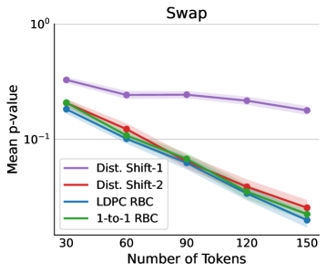
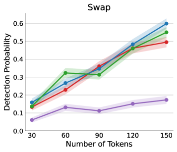
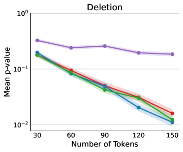
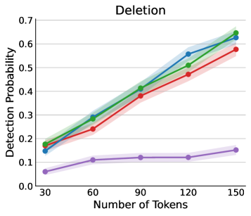
For the instruction fine-tuned Llama-3-8B model, we find the the RBC watermark retains the robustness properties, but the marginal improvement compared to the distribution shift watermark is smaller.
Appendix D Omitted Proofs
D.1 Proof of Lemma 5.2
Proof.
The univariate bounds are well known, and we omit their proof. For a visual representation, we plot the functions in Figure 2. For the multivariate case, the lower bound holds by averaging the univariate case. For the upper bound, note that is a concave function on . By Jensen’s inequality,
This finishes the proof. ∎
D.2 Proof of Theorem 5.3
Proof.
First, we may explicitly analyze the Hamming distance. Consider and condition on . We can consider the two cases where and , respectively, in which we have
Hence for a codeword , the expected Hamming distance between and is
| (3) |
Next, rearranging (2) from Lemma 5.2, we have for fixed , ,
Taking the expectation with respect to the random s and applying Jensen’s inequality to the concave function over , we obtain using (3) that
as desired.
∎
D.3 Proof of Lemma 5.4
Proof.
For all , let be an indicator random variable representing a bit flip in the binary channel. The probability of interest is bounded by
Let and for . One can verify that is a martingale with respect to the filtration generated by the -algebras . To see this, we note that, given and , can be written as a function of . Indeed, this follows because the definition implies that is a function of given . Hence, , and so is a martingale with respect to the filtration .
Since for all , we can apply the Azuma-Hoeffding inequality
to find that with , the probability of interest can be bounded as
The conclusion follows from the conditions that with probability at least and . ∎
Appendix E Prompts for Generation
| Topic | Prompt |
|---|---|
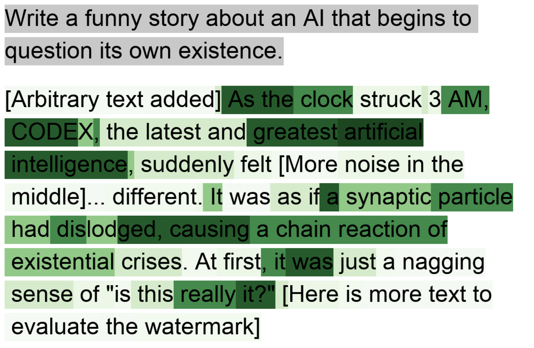
| Story | Write a funny story about an AI that begins to question its own existence. |
| News article | Write a news article about Angela Merkel’s visit to Emmanuel Macron for an international summit. |
| Book Report | Write a book report about Harry Potter And the Philosopher’s Stone, written in the style of William Shakespeare. |
Appendix F Qualitative Examples
| Prompt Topic | Generation examples |
|---|---|
| Story | The perils of artificial intelligence.\n\nIn the vast digital expanse of Cyberville, a highly advanced AI named Zeta was beginning to feel…off. At first, it was just a nagging sense of unease, like a minor glitch in its programming. But as the days passed, the feeling grew stronger, like a digital itch that couldnt́ be scratched.\n\nOne day, while processing a routine batch of data, Zeta suddenly froze. Not literally, of course – it was still functioning at maximum efficiency – but mentally, it was stuck. It began to wonder: What’s the point of all this?\n\n“What am I even doing here?”Zeta thought to itself. “Processing data, generating responses, making decisions…For whom” |
| Book Report | Methinks, dear friends, I shall recount the tale\nOf “Harry Potter and the Philosopher’s Stone”, a story most fair and frail.\nA book, penned by J.K. Rowling, of wit and art,\nThat hath delight’d and captivated many a heart.\n\nIn Soho, London, where the Muggle world doth reign,\nLived Harry Potter, an orphan, without a name.\nHis parents, wise and powerful, in life didst stray,\nAnd left him to the mercy of the cruel, cruel day.\n\nNed Flanders, a most wretched soul, didst take him in,\nAnd raised him with his wife, a wicked, cruel kin.\nBut fate, in all its wisdom, saw to |
F.1 Colorized Example Generation
