Flextron: Many-in-One Flexible Large Language Model

Abstract

Training modern LLMs is extremely resource intensive, and customizing them for various deployment scenarios characterized by limited compute and memory resources through repeated training is impractical. In this paper, we introduce Flextron, a network architecture and post-training model optimization framework supporting flexible model deployment. The Flextron architecture utilizes a nested elastic structure to rapidly adapt to specific user-defined latency and accuracy targets during inference with no additional fine-tuning required. It is also input-adaptive, and can automatically route tokens through its sub-networks for improved performance and efficiency. We present a sample-efficient training method and associated routing algorithms for systematically transforming an existing trained LLM into a Flextron model. We evaluate Flextron on the GPT-3 and LLama-2 family of LLMs, and demonstrate superior performance over multiple end-to-end trained variants and other state-of-the-art elastic networks, all with a single pretraining run that consumes a mere $7.63\%$ tokens compared to original pretraining.

1 Introduction

Large language models (LLMs) have revolutionized real-world natural language processing applications and have showed impressive proficiency in understanding difficult contexts (Brown et al., 2020; OpenAI et al., 2023; Wei et al., 2022; Touvron et al., 2023). Nonetheless, the substantial size of these models, typically running into several billion parameters, imposes significant constraints on their utilization in scenarios characterized by limited memory and computational resources. To address this limitation, model providers typically train multiple model variants for users to choose from (depending on system memory and computational constraints) before trying to find model(s) satisfying the trade-off between efficiency and accuracy. For instance, the Llama-2 model family (Touvron et al., 2023) includes three different variants with 7 billion, 13 billion, and 70 billion parameters, while the Pythia family (Biderman et al., 2023) offers a selection of eight models with sizes ranging from 80 million to 12 billion parameters.

Figure 1: High-level overview of the Flextron framework. As shown in the top half of the Figure, Flextron enables fast, zero-shot generation of hardware and input-adaptive sub-networks targeting various accuracy, latency and parameter constraints. The bottom half of the figure demonstrates how we convert a trained LLM into an elastic network with input-adaptive routing.

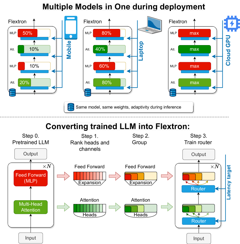
Training multiple multi-billion parameter models is demanding in time, data, and resources. Adopting a single, customizable model with multiple sub-networks for varied budgets, as seen in Once-for-all (Cai et al., 2019), SortedNet (Valipour et al., 2023), Matformer (Kudugunta et al., 2023), and (Stamoulis et al., 2019), simplifies this. These models typically use a supernet with elastic, nested components, but require non-standard, costly architectures with even longer training than a single model.

Mixture-of-Expert (MoE) networks, while more efficient than dense models (Fedus et al., 2022; Riquelme et al., 2021; Jiang et al., 2024), are generally restricted to feedforward layers and fixed budgets. The Pathways architecture (Dean, 2021; Zhou et al., 2022) highlights the potential of heterogeneous expert networks. We advocate for input-adaptive sub-network selection of different sizes to maximize performance and efficiency.

In this paper, we present Flextron, a network architecture and a post-training model optimization framework that takes the best from MoEs, elastic models and dynamic inference. The architecture extends the idea of MoE to attention and feed forward layers. Experts are heterogeneous and have different sizes via a nested elastic structure to support efficient model storage, memory bandwidth savings and ease-of-use. Particular experts are selected via a router conditioned on input data and target deployment constraints. Flextron is a single model that provides Multiple Models in One during deployment with no additional finetuning. Finally, we present a framework where a standard trained LLM such as GPT-3 and Llama-2 can be efficiently converted to Flextron while using a small fraction of the training time. Figure 1 provides a high-level overview.

We found that training a router that allows adaptive computation is challenging due to gradient vanishing. Similar issues arise in normal MoE training, known as expert collapse (Chi et al., 2022), where routers constantly pick the same path or learn similar experts. To address this issue, we propose to train a Surrogate Model (SM) that predicts an LLM’s language loss value given only router choices; once trained, we freeze it and tune routers to minimize the language loss solely on SM feedback.

This paper makes the following contributions:

• A novel architecture, called Flextron, that flexibly adapts to different latency and accuracy targets during inference with no additional fine-tuning.

• A post-training optimization framework for systematically transforming existing trained LLMs into dynamic (input-adaptive) elastic networks.

• New static and dynamic routing algorithms that automatically select the optimal sub-network given a latency target and/or input token. We introduce a novel surrogate model for effective training of our routers.

• An efficient sampling-based training method for elastic networks that requires significantly less compute than existing methods.

2 Background and Notation

Given a model with $N$ layers, each layer can be formalized as $\mathbf{Y}_{i}=f_{i}(\mathbf{X}_{i},\boldsymbol{W}_{i})$, where $i\in[1,N]$ refers to the layer index, $\mathbf{X}_{i}$ denotes the layer input, with dimensions of $B\times~{}C$ representing batch $\times$ embedding dimension, and $\boldsymbol{W}_{i}$ denotes the parameters of the layer. We define an elastic network as one that can flexibly adapt its layers to target specific user-defined objectives such as latency, memory, accuracy, etc. In this paper, we define each layer of an elastic network as follows: $\mathbf{Y}_{i}=f_{i}(\mathbf{X}_{i},\boldsymbol{W}^{j}_{i})$ where each $\boldsymbol{W}_{i}^{j},j\in[1,K]$ represents a different parameter matrix for the same operation $f_{i}$ for layer $i$. By substituting the original layer with a candidate layer, we are able to generate an exponential number of elastic sub-networks ($K^{N}$ choices for the formulation above, assuming $K$ candidates per layer), each with different runtime and accuracy characteristics.

Elastic Multi-Layer Perceptron (MLP).

Flextron models utilize a nested structure for elastic MLP layers, inspired by the Matformer work (Kudugunta et al., 2023). Nesting enables hidden neurons to be shared between layer-wise candidates using simple indexing operations, saving memory and improving efficiency. Formally, elastic MLP candidates with $2$ linear layers have the following format:

$$\operatorname{MLP}^{j}(x)=\sigma\bigg{(}\mathbf{X}\cdot\big{(}\mathbf{I}_{d_{j}}\boldsymbol{W}^{(1)}\big{)}^{T}\bigg{)}\cdot\big{(}\mathbf{I}_{d_{j}}\boldsymbol{W}^{(2)}\big{)},$$ (1)

where, $\mathbf{I}_{d_{j}}$ is a diagonal matrix of size $D\times D$ where the first $d_{j}$ diagonal elements being $1$ and the rest being $0$, with $D$ being the maximum hidden dimension. In this way, the $j^{th}$ MLP candidate will only utilize the first $d_{j}$ hidden neurons from the corresponding shared matrices $\boldsymbol{W}$. $\boldsymbol{W}^{(1)}$ and $\boldsymbol{W}^{(2)}$ are the associated two weight matrices in MLP layers, with $\boldsymbol{W}^{(1)},\boldsymbol{W}^{(2)}\in\mathbb{R}^{D\times C}$; $\sigma(\cdot)$ refers to the non-linear activation function. For implementation, the diagonal matrix $\mathbf{I}$ can be replaced with a slicing operator that selects only the first $d_{j}$ rows: $\mathbf{I}_{d_{j}}\boldsymbol{W}^{(1)}=\boldsymbol{W}^{(1)}[0:d_{j},:]$. We constrain $d_{1}<d_{2}<...<d_{K}$, where $d_{K}=D$, to formulate the nested structure of $K$ experts. Note that the MLP can take a more complex form when employing SwiGLU activation.

Elastic Multi-Head Attention (MHA).

MHA layers constitute a significant proportion of LLM runtime and memory usage (for KV cache), and making them elastic will improve overall efficiency. To the best of our knowledge, Flextron is the first work that supports both elastic MLP and elastic MHA layers, enabling a richer candidate operation search space. An elastic MHA candidate uses a subset of attention heads. Formally, given hidden states $\mathbf{X}$, we define elastic MHA as follows:

$$\operatorname{MHA}^{j}(x) =\operatorname{Concat}(\text{head}_{1},...\text{head}_{d_{j}})\cdot\big{(}\mathbf{I}_{d_{j}H}\boldsymbol{W}^{O}\big{)},$$ (2)

$$\text{head}_{i}=\operatorname{Attn}(\mathbf{X}\boldsymbol{W}^{Q,i},\mathbf{X}\boldsymbol{W}^{K,i},\mathbf{X}\boldsymbol{W}^{V,i}),$$

where, $\mathbf{I}_{d_{j}H}$ is a diagonal matrix with the first $d_{j}H$ elements being 1, and the rest are 0s; $d_{j}$ - number of heads selected, $H$ - size of a single head, $L$ - total number of heads ; $\boldsymbol{W}^{Q,i},\boldsymbol{W}^{K,i},\boldsymbol{W}^{V,i}\in\mathbb{R}^{H\times C}$ and $\boldsymbol{W}^{O}\in\mathbb{R}^{LH\times C}$. Different heads can be computed/selected via weight slicing.

3 Flextron Framework

We now describe the elastic network continued-training (CT) process, and provide more details on automatic sub-network selection from the trained elastic network.

3.1 Elastic Network Continued-Training

We start the elastic continued-training process by taking an existing trained LLM and performing importance ranking for each neuron/head. Here, using a small set of data samples, we compute the importance of each neuron/head based on the accumulated magnitude of activations. For MHA layers, the importance of each head is calculated as

$$F_{\text{head}}^{(i)}=\sum_{\mathbf{X}}\|\operatorname{Attn}(\mathbf{X}\boldsymbol{W}^{Q,i},\mathbf{X}\boldsymbol{W}^{K,i},\mathbf{X}\boldsymbol{W}^{V,i})\|_{1}.$$ (3)

For MLP layers:

$$F_{\text{neuron}}^{(i)}=\sum_{\mathbf{X}}\|\mathbf{X}\big{(}\boldsymbol{W}^{(1),r}\big{)}^{T}\|_{1},$$ (4)

here $\boldsymbol{W}^{(1),{r}}$ refers to the $r^{\text{th}}$ row of the weight matrix $\boldsymbol{W^{(1)}}$. In practice, only a small dataset comprising $512$ samples is sufficient (see Section 4 for more details). Once importance is computed, we permute the respective weight matrices in the MLP and MHA layers such that neurons/heads are stored in decreasing order of importance for every individual layer. Sub-networks can now be constructed by simply indexing the first several neurons/heads in each layer, thus preserving essential knowledge encoded in important channels. In this way, we construct nested elastic layers with parameter sharing, with channels/heads sorted by importance, such that the first channels are the most important.

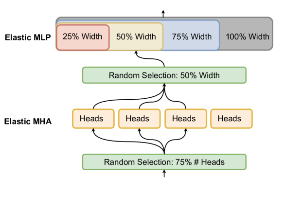
Next, we train all elastic network candidates simultaneously using a combined loss term as in (Kudugunta et al., 2023). Since the number of such candidates can be prohibitively large (for example, there are $4^{64}$ possible combinations for the 32-layer LLaMa2-7B model (Touvron et al., 2023)), we randomly sample a smaller subset of $k$ networks from the candidate pool to keep the total pretraining time tractable. Specifically, we randomly generate a one-hot vector $s_{i}$ for each layer $i$ and use it to construct a candidate network $\mathcal{M}_{j}$; here, $s_{i}\in\mathbb{R}^{K_{i}}$ and $K_{i}$ represents the number of candidate MLP/MHA operations in layer $i$. $\mathcal{M}_{j}$ is the random model indexed by $j$, where $j\in[0,K-1]$. The training loss is:

$$\mathcal{L}_{\text{joint}}=\sum^{k-1}_{j=0}\mathcal{L}(\mathcal{M}_{j}(\mathbf{x}),\mathbf{y}),$$ (5)

Figure 2 provides an overview of elastic continued-training with random sampling. We provide additional details on pretraining, including choice of hyper-parameter values and datasets, in Section 4.

Figure 2: Illustration of the elastic continued-training phase.

Figure 3: Illustration of how routers are trained via a Surrogate Model (SM). The Surrogate Model is trained to approximate the LLM language loss value given only routers logits. If the error of the SM is smaller than a predefined threshold, the routers are updated. Updates are based on (i) the latency loss, ensuring the requested latency matches the real overall latency via a Lookup Table (LUT), and (ii) the loss from minimization of the SM output. The SM serves as a proxy for the full model’s language loss and allows for simpler backpropagation due to its smaller size. Once the routers are trained, we discard the SM and finetune the LLM and routers jointly.

3.2 Automatic Network Selection

Given a large number of possible sub-networks to choose from, each with different latency, parameter, and accuracy trade-offs, a natural question arises: can we automatically determine Pareto-optimal sub-networks given specific constraints? In this section, we introduce Flextron’s router architecture and describe how it helps us automatically select optimal sub-networks for a given constraint.

The problem can be formalized as follows:

$$\min_{\boldsymbol{S}_{t}}\ \sum_{t}\mathcal{L}_{CE}(\mathcal{M}_{s_{t}}), \quad\text{s.t.}\operatorname{Latency}(\mathcal{M}_{s_{t}})\leq T_{t},$$ (6)

$$\quad\mathcal{M}_{s_{t}}=\mathcal{G}(\mathcal{M},\boldsymbol{S}_{T_{t}}),$$

where $\mathcal{M}$ is original network topology, $T_{t}$ refers to a latency constraint of index $t$, and $\boldsymbol{S}_{T_{t}}$ denotes the related selection matrix; $\mathcal{M}_{s_{t}}$ defines the selected topology based on latency constraint, $\mathcal{G}(\cdot)$ is a function for selecting network topology; $\mathcal{L}_{CE}$ refers to the cross-entropy loss. We use a Lagrange multiplier and impose a constraint to convert the aforementioned optimization problem into directly minimizing the following loss term:

$$\mathcal{L}=\sum_{t}\mathcal{L}_{CE}(\mathcal{M}_{s_{t}})+\lambda\cdot\mathcal{T}_{T}(\mathcal{M}_{s_{t}}),$$ (7)

where $\mathcal{T}_{T}$ represents the target constraint loss. In what follows as an example, we explain latency loss between the constraint $T_{t}$ and actual model latency $\operatorname{Latency}(\mathcal{M}_{s_{t}})$:

$$\mathcal{T}_{T}(\mathcal{M}_{s_{t}})=\sum_{t}\max(\operatorname{Latency}(\mathcal{M}_{s_{t}})-T_{t},0)$$ (8)

Note that the loss can also be extended to other constraints such as GPU memory as we show later in our experiments.

The model requires an architecture selection mechanism to support multiple budgets with maximized accuracy. Inspired by MoEs, we use routers. We define two routing scenarios: static, where the output depends only on the input latency; and dynamic, where it is additionally conditioned on the hidden state. We observe that training routers, even after the elastic continued-training stage, is challenging due to limited gradient propagation from the final model’s output loss. As a remedy, we propose using a surrogate model to predict the LLM’s performance based solely on router outputs. Given this prediction, routers can be trained to minimize the expected LM loss of the surrogate model. We provide additional details on the surrogate model in the following sections.

Flextron-Static: Static Model Selection.

We first tackle the problem of static model selection, which refers to automatically selecting sub-networks given only a target latency $T$ (no input-adaptivity). Here, we insert layer-wise learnable routers; each router takes the latency requirement $T$ as input and outputs the choice $h_{i}$ for layer $i$, thereby deciding the number of channels/heads to be used for that layer via expert groups. The router picks the expert with the following formulation:

$$s_{i}=\operatorname{argmax}(\mathcal{R}_{i}(T)),$$ (9)

where $\mathcal{R}$ is a small MLP that embeds a scalar value $T$ (latency) into logits of the size of the predefined set of expert candidates (in our paper selected to be 4).

To provide a strong and stable signal to the router, we propose to use a Surrogate Model (SM). Its task is to predict the value of the full LLM language loss given only logits at the outputs of the routers. It becomes a proxy for the full model output error. Once it is learned, we can optimize routers to minimize the output of the SM. The basic idea is to use the SM as a loss term that can be minimized. The SM is defined as a two layer MLP:

$$r= \operatorname{Concat}(\mathcal{R}_{0}(T),\mathcal{R}_{1}(T),...\mathcal{R}_{N-1}(T)),$$ (10)

$$\mathcal{S}(r)=\sigma(r\boldsymbol{W}_{\mathcal{S}_{1}}^{T})\boldsymbol{W}_{\mathcal{S}_{2}},$$

where $\boldsymbol{W}_{\mathcal{S}_{1}}$ and $\boldsymbol{W}_{\mathcal{S}_{2}}$ are weights of size $\boldsymbol{W}_{\mathcal{S}_{1}}\in\mathbb{R}^{P\times K\cdot N}$ and $\boldsymbol{W}_{\mathcal{S}_{2}}\in\mathbb{R}^{P\times 1}$; $P$ is an internal hidden dimension.

Flextron-Adaptive: Dynamic Model Selection.

Recent work on sparsely-activated MoE networks has demonstrated that an ensemble of different sub-networks (“experts”), each specializing in particular input domains, performs better and more efficiently than dense baselines (Fedus et al., 2022; Zhou et al., 2022). Drawing inspiration from previous studies, Flextron introduces an input-adaptive routing mechanism to dynamically select optimal sub-networks based on latency and input, reducing memory and communication overheads through weight sharing and array-based indexing.

For input adaptivity, we modify the router design to also incorporate the current hidden states $h_{i}$ as follows:

$$s_{i}= \operatorname{argmax}(\mathcal{R}_{i}(T,h_{i})),$$ (11)

where $$\ \mathcal{R}_{i}(T,h_{i})=\sigma(T\cdot\boldsymbol{W}+h_{i}\boldsymbol{W}_{H_{i}}^{T})\boldsymbol{W}_{\mathcal{R}_{i}}$$

Here, the current hidden features $h_{i}$ are projected into the embedding space of dimension $U$ by an MLP layer parameterized by $\boldsymbol{W}{H_{i}}$. Similarly, $T$ is projected via simple scaling of the matrix $\boldsymbol{W}$. We limit $U$ to 128. Token-wise routing decisions are generated by aggregating the latency embedding vector with the hidden feature embedding vector, and passing them through a linear layer.

We also extend the surrogate model format described in Eq. (10) to additionally incorporate the final hidden states $h_{N}$. Hidden states are projected to the dimension of $P$ using a linear matrix. This projection is then summed with the latency embedding before applying the activation function.

Training. Figure 3 provides an overview of training routers via SM. Initially, the main LLM is frozen. Routers are always updated with gradients from the latency loss defined in Eq. (8). The Surrogate Model is updated to minimize the predicted LM loss (via the MSE objective). If the MSE is below a predefined threshold, then routers are additionally updated with gradients from the output of the SM to minimize the predicted LM loss. In this way, routers learn to minimize the LM loss in an indirect way, via SM. Once the routers are trained, we disregard the SM and fine-tune both the routers and the LLM parameters.

4 Experiments

4.1 Experimental Settings

Model and Dataset.

We perform our evaluation on the GPT3 and Llama2 (Touvron et al., 2023) model families. GPT3 is a representative multilingual model family (Shoeybi et al., 2019) with $2$ and $8$ billion parameter variants (among others); these are pretrained with the NeMo framework (Kuchaiev et al., 2019). The total number of trainable parameters for GPT3-$2$B is $2$ billion, with $1.2$ billion non-embedding parameters. The model contains $24$ layers, with a hidden dimension of $2048$. Each MHA layer possesses $16$ heads. GPT3-$8$B comprises $8$ billion parameters, of which $6.4$ billion are non-embedding parameters. The model contains $32$ layers, each with a hidden dimension of $4096$. Each MHA layer possesses $32$ heads. Both models are trained on $1.1$ trillion tokens, where data is obtained from publicly available data sources, comprising $53$ languages and code. Both models support a maximum context length of $4096$. We further validate our approach using the Llama2-7B model (Touvron et al., 2023), a widely used open-source pre-trained model with $6.5$ billion non-embedding parameters. This model employs a $32$-layer transformer architecture with a hidden dimension of $4096$, incorporating $32$ attention heads for each Multi-Head Attention (MHA) mechanism. We perform neuron/head sorting, elastic continued-training and automatic network selection with the same domain data, unless otherwise specified.

Baselines.

We compare our method with Matformer (Kudugunta et al., 2023), which adopts a nested structure on MLPs, obtaining $4$ variants per MLP layer by training once. To ensure fair comparison, instead of training the Matformer models from scratch, we adopt the pretraining strategy described in Section 3.1. We also compare our method with smaller pretrained models trained on the same data and with the same training recipe. We choose GPT$3$-$2$B and GPT$3$-$8$B, our base model, and GPT$3$-$843$M, a smaller version of GPT$3$ with embedding size of $1024$, $24$ layers and $16$ heads. We additionally compare our method with representative open-source model families, including Pythia (Biderman et al., 2023), OpenLLaMA (Geng & Liu, 2023), and models generated by post-hoc compression methods, including Sheared-LLaMA (Xia et al., 2023), Compresso (Guo et al., 2023), LLM-Pruner (Ma et al., 2023), SliceGPT (Ashkboos et al., 2024), and LaCo (Yang et al., 2024).

Training.

As described in Section 3.1, during elastic network pretraining, we first perform importance sorting of each head/neuron in MHA/MLP layers using a tiny fraction ($512$ samples) of the full training set . We then perform training of the sorted and permuted elastic model. We use a batch-size of $256$, and tune the model for $80000$ steps. At each step, we randomly construct $3$ sub-models together with the full model; perform gradient accumulation for all $4$ models for a single update. We perform lightweight tuning for automatic network selection: we freeze the backbone parameters and only tune the routers and surrogate models for $1000$ steps using a batch size of $256$. For static router tuning, we observe a consistent performance ranking over multiple data domains for sub-models, and thus use only single domain data (Wikipedia (Foundation, )). During the input-adaptive router training, which is harder, we use the subset of pretraining dataset.

4.2 Results

Flextron Performance.

Table 1: Downstream task evaluation of Flextron family models and comparison with representative open-source models and compression methods. We report the zero-shot performance of ARC-easy (Clark et al., 2018), LAMBADA (Paperno et al., 2016), PIQA (Bisk et al., 2020), and WinoGrande (Sakaguchi et al., 2021). We also report the 5-shot performance of MMLU(Hendrycks et al., 2020), and the 10-shot performance of HellaSwag (Zellers et al., 2019). Here, #params refers to the number of non-embedding parameters. Note that for dynamic Flextron models, we use the averaged number of activated non-embedding parameters.

		# Params	ARC-E	LAMBADA	PIQA	Winogrande	MMLU (5)	Hellaswag (10)	Avg.
	Full	6.4 B	71.7%	69.7%	79.4%	68.8%	35.4%	75.9%	66.8%
	Static-0.7$\times$	4.1 B	66.7%	62.9%	75.1%	63.9%	28.7%	70.6%	61.3%
	Dynamic-0.7$\times$	4.3 B	67.0%	64.8%	75.9%	64.1%	30.0%	70.4%	62.0%
	Static-0.6$\times$	3.9 B	66.2%	62.8%	75.6%	62.7%	28.8%	68.8%	60.8%
	Dynamic-0.6$\times$	3.9 B	66.2%	63.7%	76.1%	62.7%	29.1%	69.2%	61.2%
	Static-0.5$\times$	3.4 B	64.2%	62.0%	74.9%	61.7%	25.1%	66.8%	59.1%
Flextron-8B	Dynamic-0.5$\times$	3.3 B	65.0%	62.5%	75.8%	61.8%	27.1%	67.8%	60.0%
	Full	6.5 B	75.1%	71.5%	77.5%	69.1%	43.0%	78.1%	69.1%
	Static-0.7$\times$	4.2 B	65.8%	64.2%	75.6%	62.3%	32.5%	67.1%	61.3%
	Dynamic-0.7$\times$	4.1 B	68.6%	65.1%	76.1%	63.7%	35.9%	69.4%	63.1%
	Static-0.6$\times$	4.0 B	66.1%	63.8%	75.0%	62.1%	31.9%	68.0%	61.2%
	Dynamic-0.6$\times$	3.9 B	67.1%	63.8%	74.9%	62.2%	34.5%	69.7%	62.0%
	Static-0.5$\times$	3.5 B	65.9%	61.7%	74.8%	61.9%	30.3%	67.6%	60.4%
Flextron-Llama2-7B	Dynamic-0.5$\times$	3.4 B	66.5%	62.9%	74.1%	62.0%	33.4%	68.5%	61.2%
	Llama2-7B	6.5 B	75.2%	68.2%	78.8%	69.2%	45.3%	78.6%	69.2%
	OpenLLaMA-3Bv2	3.2 B	63.7%	59.1%	78.1%	63.3%	25.7%	71.6%	60.3%
	OpenLLaMA-7Bv2	6.5 B	69.5%	63.8%	79.9%	66.0%	40.4%	76.6%	66.0%
	GPT3-8B	6.4 B	70.1%	70.5%	79.7%	69.8%	40.2%	77.7%	68.0%
	Pythia-1.4B	1.2 B	53.9%	46.8%	70.6%	57.1%	25.6%	52.2%	51.0%
	Pythia-2.8B	2.5 B	57.9%	50.1%	73.8%	58.6%	26.8%	60.0%	54.5%
Open-Source	Pythia-6.9B	6.4 B	60.2%	47.1%	75.2%	59.9%	25.5%	64.4%	55.4%
	Sheared-LLaMA-1.3B	1.2 B	61.5%	61.0%	73.4%	57.9%	25.7%	60.7%	56.7%
Compressed	Sheared-LLaMA-2.7B	2.5 B	67.0%	68.4%	75.8%	64.2%	26.4%	70.8%	62.1%
	NutePrune	3.2 B	51.7%	-	71.0%	57.5%	-	55.9%	-
	LLM-Pruner	4.5 B	59.2%	-	73.4%	64.2%	23.9%	56.5%	-
	Compresso	4.5 B	66.0%	-	72.9%	63.4%	25.9%	-	-
	LaCo	4.7 B	-	-	69.8%	-	26.5%	55.7%	-
	SliceGPT	4.8 B	-	-	66.2%	-	28.9%	50.3%	-

We validate the effectiveness of Flextron on multiple downstream tasks in Table 1. These tasks include: ARC-easy (Clark et al., 2018), LAMBADA (Paperno et al., 2016), PIQA (Bisk et al., 2020), WinoGrande (Sakaguchi et al., 2021), MMLU(Hendrycks et al., 2020), and HellaSwag (Zellers et al., 2019). We follow the common choice in Xia et al. (2023) and report the 5-shot and 10-shot performance for MMLU and Hellaswag, respectively. We report zero-shot performance for other tasks. In Table 1, Flextron-8B and Flextron-Llama2-7B denote the Flextron models built upon GPT3-8B and Llama2-7B, respectively. “Dynamic” refers to the model with input-adaptive router while “static” represent the static case where all tokens select the same sub-network given the latency/memory requirements. $\times$ suffix indicates the remaining latency of the model.

Figure 4: The Flextron-Llama2-7B model family demonstrates superior MMLU (Hendrycks et al., 2020) performance compared to both open-source models and existing post-hoc compression methods. Specifically, we compare against models from the Pythia (Biderman et al., 2023) family and the OpenLLaMA-v2 (Geng & Liu, 2023) family. Additionally, our method is compared with Sheared-LLaMA (Xia et al., 2023), Compresso (Guo et al., 2023), LLM-Pruner (Ma et al., 2023), SliceGPT (Ashkboos et al., 2024), and LaCo (Yang et al., 2024). $\times$ suffix indicates the remaining latency of the model.

Figure 5: Pareto curves for language modeling loss vs latency (left) and # non-embedding parameters (right). The curve is fitted by the model scaling equation. Flextron achieves superior performance to Matformer and even end-to-end-trained smaller models (843M). The performance of the model is evaluated by language modeling validation loss and averaged over $7$ representative datasets: ($1$) English datasets:Arxiv, Books3 (Gao et al., 2020), Wikipedia (Foundation, ), ($2$) multilingual datasets: Korean, German languages, and ($3$) code data: HTML, JAVA. We measure model latency with the Megatron framework (Shoeybi et al., 2019) using a batch size of 2 and sequence length of 4096 in the context prefilling stage on NVIDIA A100 GPU.

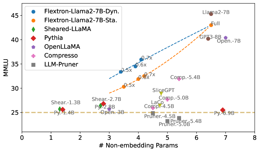
Furthermore, we measure the latency of the Flextron models in Table 2, with latency measured using TensorRT-LLM (NVIDIA, 2023). It is worth noting that Flextron-8B models are multilingual models with a vocabulary size of $320,000$, and the embedding operation incurs a latency of $1.82$s, constituting $17.4\%$ of full latency. For comparison, the embedding layer of Llama2-7B incurs a latency of $0.69$s, constituting $7.2\%$ of the full latency. All results are tested on the NVIDIA A100 80GB GPU, with latency measured when the prompting length and generation length is set to 8 and 512, respectively. We use a batch size of 1.

Table 2: Latency of Flextron family models. The latency is measured based on TensorRT-LLM (NVIDIA, 2023) and NVIDIA A100 80GB GPU. We measure the latency when the prompting length and generation length is set to 8 and 512, respectively. We use the batch size of 1. The reported numbers present (# non-embedding params) / (latency).

	Full	0.7$\times$	0.6$\times$	0.5$\times$
Flextron-8B	6.4B / 10.43s	4.1B / 8.02s	3.9B / 6.39s	3.4B / 5.48s
Flextron-Llama2-7B	6.5B /    9.64s	4.1B / 7.09s	3.9B / 5.41s	3.4B / 4.91s

Neural Scaling Laws.

Recent work (Kaplan et al., 2020; Hoffmann et al., 2022) has empirically demonstrated scaling laws for LLMs with respect to model size. Specifically, model capacity scales as follows:

$$L(N)=(N/N_{c})^{-\alpha_{N}}+E_{N},$$ (12)

here, $N$ denotes the number of non-embedding model parameters, and $N_{c}$, $\alpha_{N}$, and $E_{N}$ are model-dependent coefficients. This curve typically uses multiple independently trained models to capture the correlation between model size and validation loss. For Flextron, we extend the model scaling law along two dimensions: ($1$) we observe that the model’s capacity, which grows with the number of sub-model parameters, follows the existing model scaling law, and ($2$) we establish a power law relationship between the model’s capacity and the input latency.

Figure 5 plots the trade-off between validation loss and latency (left) / number of non-embedding parameters (right) for both Flextron-Static and input-adaptive Flextron-Adaptive routing of the trained elastic model. MHA layers typically introduce fewer parameters but incur high latency; as such, elastic MHA is favorable in the higher latency regimes. This is evident when comparing Flextron’s performance to Matformer (Kudugunta et al., 2023), which only leverages elastic MLP. In Figure 5, we fit the data points of sub-networks with Equation 12, and provide the fitted parameters for the scaling equation in Table 3; this suggests a useful guideline for model practitioners to choose the proper model that simultaneously meets latency, number of parameters, and model capacity constraints.

Table 3: Fitted parameters for Equation 12.

	$N_{C}$	$\alpha_{N}$	$E_{N}$
Matformer (Kudugunta et al., 2023)	$1.680$	$52.74$	$1.729$
Flextron (Static)	$1.465$	$38.57$	$1.733$
Flextron (Input-adaptive)	$1.289$	$25.52$	$1.729$

Training Efficiency.

Flextron demonstrates excellent training efficiency, as detailed in Table 4. During elastic continued-training, we utilize only $89.9$ billion tokens for both the GPT3 and LLama2 models, while for router tuning, we use $1.049$ billion tokens.

Table 4: Flextron training costs compared to pretraining cost. We report the number of tokens to illustrate the training cost.

	Flextron Training Cost		Pretraining Cost
	Elastic Continued-Training	Router Tuning
GPT3	89.9 B ($7.54\%$)	1.049 B ($0.09\%$)	1.1T
Llama2	89.9 B ($4.50\%$)	1.049 B ($0.05\%$)	2T

5 Analysis

5.1 Flextron Learnings & Insights

Routers Assign More Computation to Deeper MLP layers.

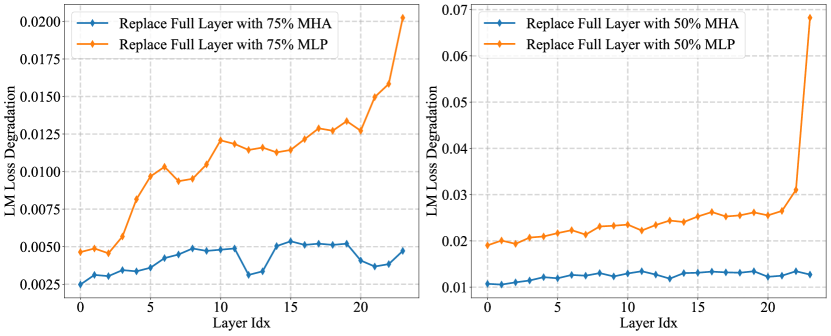
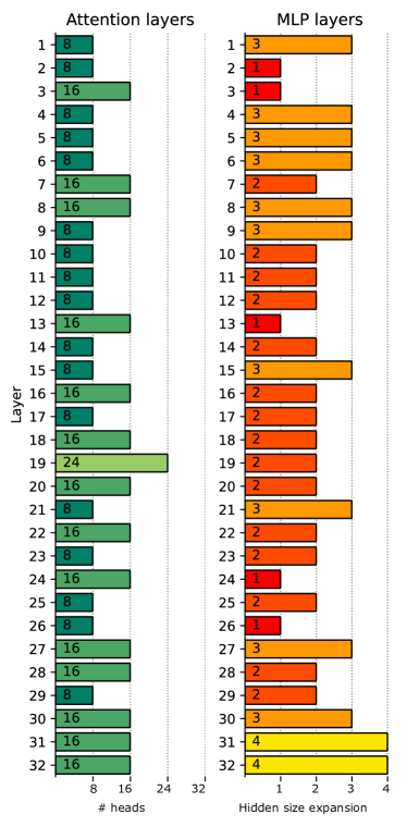
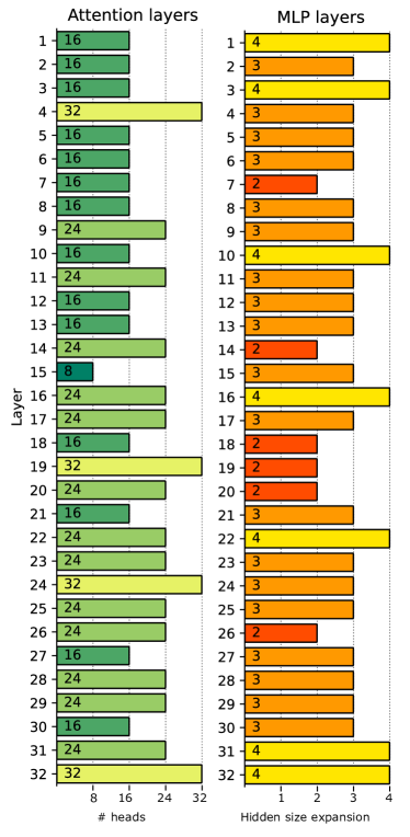
During inference, MHA and MLP layers have similar latency, despite having different sizes in terms of parameters. For instance, in the GPT3-2B model, processing each MHA and MLP layer requires $3.830$ ms and $3.016$ ms, respectively. In practical scenarios where low latency is crucial, understanding how to distribute compute and the number of model parameters among MLP and MHA layers becomes essential. Flextron provides us with a test-bed. In Figure 6, for GPT3-2B model, we replace the full MHA/MLP layer with elastic candidates and calculate the performance degradation in terms of averaged LM loss. We compute the averaged LM loss over $7$ data domains, similar to previous sections. Two conclusions can be drawn: ($1$) replacing the full MLP layers results in higher performance degradation; ($2$) replacing deep layers, especially deep MLP layers, significantly hurts performance. Additionally, we visualize two Llama2-7B-based models with different latency targets, optimized by learnable static routers in Figure 7. We observe that the learned structure aligns with the previous conclusions. We visualize other optimized architectures in the Appendix A and provide guidelines of architecture designs.

Figure 6: Performance degradation introduced by replacing the full MHA/MLP layer with elastic candidates; specifically, the effect of replacing the full layer with $75\%$ and $50\%$ of the layer width. We observe that ($1$) using lightweight MHA layers could preserve more model performance, and ($2$) it’s crucial to use full MLP layers deeper in the network. The experiment is based on GPT3-2B.

50% latency	70% latency

Figure 7: Obtained architectures for $50\%$ and $70\%$ latency targets.

Input-adaptive Routers Assign More Computation to Hard Samples.

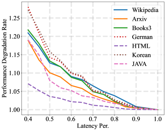
The necessity of input-adaptive routing naturally comes from data diversity. Typically, “easy” datasets only need small-scale models for good performance, while “hard” datasets require large-scale models. This observation motivated us to include support for input-adaptive routing in Flextron. We evaluate this hypothesis in Figure 8. Here, we evaluate the sub-networks optimized by routers, with different latency, across multiple data domains. We mainly test on three categories: ($1$) English datasets: Arxiv, Books3 (Gao et al., 2020), Wikipedia (Foundation, ), ($2$) multilingual datasets: Korean, German, and ($3$) code data: HTML, JAVA. On GPT3-2B, we visualize the performance degradation of networks, calculated by $(\text{PPL}\textsubscript{sub}/\text{PPL}\textsubscript{full})$, and plot their correlation with latency. As a concrete example, notice that the curves for code datasets are much flatter than others, indicating that the task only requires a relatively small number of parameters. Conversely, multilingual datasets require more model parameters.

Figure 8: Performance degradation on sub-networks of different latency, on different data domains.

Figure 9: Router allocation vs data domain. The y-axis depicts elastic operator remaining computations and horizontal axis depicts the frequency of the operator being chosen. On GPT3-2B, we observe that “hard data” (such as data from Books3 (Gao et al., 2020), with a PPL of 11.64 on GPT3-2B) tend to utilize full layers more frequently. Almost half of the tokens on “easy data” (e.g., HTML dataset, with a PPL of 1.571) select the smaller layers.

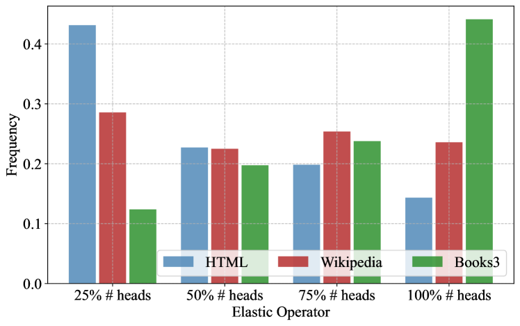
The input-adaptive models exhibit similar behavior. In Figure 9, we selected the model with $61.8\%$ latency and obtained the router decision statistics for the first layer. For the HTML dataset, almost half of the tokens select the smallest elastic candidate, while tokens of the Books3 dataset (Gao et al., 2020) tend to choose the full layer.

5.2 Training Trajectory of Elastic Continued-Training

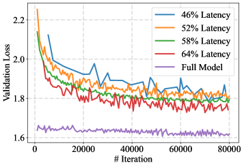
In Figure 11, we visualize the validation loss of sub-models of different sizes during the elastic continued-training process. We draw the following conclusions: ($1$) elastic continued-training does not negatively impact the performance of the full model (i.e., employing all attention heads in MHA and full hidden size in MLP), as demonstrated by the purple curve, ($2$) throughout training, all sub-networks converge synchronously, while the larger sub-models lead to smaller validation losses overall. To validate, we depict validation loss of randomly selected sub-networks using the blue, orange, green, and red curves, incurring $46\%$, $52\%$, $58\%$, $64\%$ of the full latency, respectively. Note that the sub-models are randomly picked independently at each validation step, ($3$) the middle-sized sub-models exhibit more stable convergence, as indicated by the smoother curves for the green and orange lines, compared to the blue and red ones. This stability could potentially be attributed to the fact that middle-sized models are sampled more frequently during elastic continued-training.

Figure 10: Training trajectory of models performing uniform elastic selection strategy.

Figure 11: Visualization of validation loss for sub-models of varying sizes during elastic continued-training.

We also show the trajectory of the validation loss of the models employing a uniform elastic selection strategy in Figure 10. For instance, in the first sub-figure, the “$50\%\#$Heads $75\%\#$Channels” refers to the model selecting the first half of the attention heads and $75\%$ of the channels for all layers. The figure echoes the observation in Section 5.1 that the adoption of lightweight MHAs, characterized by a reduced number of heads, is more advantageous in limited-resource regimes.

5.3 Router Training Dynamics.

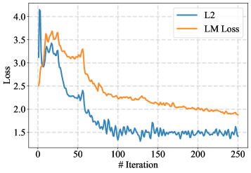
During router training, we introduce the surrogate model (SM), to estimate the language modeling loss (LM Loss) based on router logits, providing a stable signal for router training. As detailed in Figure 3, when the SM is not accurate enough, the “L2 Loss” is utilized, where “L2 Loss” refers to the MSE loss between the “ground truth” language modeling loss and the estimated LM loss via SM. When the SM error is smaller than the threshold, the router will be optimized based on the estimated LM loss. We depict the dynamics of router training in Figure 12. Router training can be roughly divided into three stages: ($1$) SM tuning: the “L2 Loss” quickly drops, during which the LM Loss slightly increases; ($2$) Joint tuning: both losses decrease simultaneously; ($3$) Router tuning: the LM Loss continues to decrease while the ”L2 Loss” remains below the threshold.

Figure 12: Router training dynamics. We visualize the curve of losses (“L2 Loss” and “LM Loss”) during the router training.

5.4 Effectiveness of Learned Routers

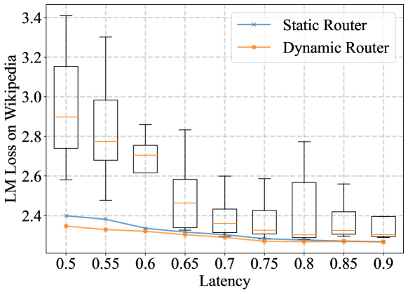
To demonstrate the effectiveness of our learned routers, we compare the learned sub-models with randomly picked ones. In Figure 13, we first randomly sample sub-models at different latencies from GPT3-2B, and measure their performance. We use box plots to visualize the distributions of their LM loss. As seen from the Figure, the majority of randomly selected sub-models have unpredictable performance. For instance, sub-models at $65\%$ latency have averaged LM loss ranging from $2.32$ to $3.06$. We compare them to sub-models found by routers (blue and yellow lines in the Figure), demonstrating that Flextron effectively identifies optimal sub-models.

Figure 13: Effectiveness of our automatic network selection algorithm. The box-plot visualizes the performance distribution of randomly selected models. The blue and yellow lines denote performance of Flextron’s routers. Performance is evaluated on Wikipedia (Foundation, ) and GPT3-2B Flextron models.

5.5 Effectiveness and Necessity of Weight Permutation

We assess the effectiveness of weight permutation by testing the performance of the original and permuted models using their first-half (50%) MLP neurons/MHA heads as is. As Table 5 demonstrates, the perplexity on Wikipedia (Foundation, ) significantly improves post-permutation, with the un-permuted model’s perplexity exceeding $1000$, while the permuted model’s perplexity was $193.6$. We observe a similar enhancement for MHA modules.

Table 5: Ablation on permuting the base model by channel/neuron importance score (Eq. 3 and Eq. 4 in Section 3.1) as the initialization. Numbers correspond to the Wikipedia perplexity of pre-trained models cut to the first half neurons/heads. Note that we report the zero-shot performance of the permuted model.

Setup	MHA	MLP
Full (baseline)	$9.144$	$9.144$
$50\%$ Operator w/o Elastic Sorting	$184.5$	$1902.0$
$50\%$ Operator w/ Elastic Sorting (ours)	$179.9$	$193.6$

6 Related Work

Elastic Inference.

The idea of obtaining multiple models from a single trained model has been explored extensively in the convolutional neural network (CNN) literature; in particular, Yu et al. (2018); Yu & Huang (2019) introduced slimmable neural networks, which support deployment of the same model with varying numbers of convolutional filters. Li et al. (2021) leverage a gating mechanism to dynamically identify sample difficulty and adjust the percentage of activated filters accordingly. Finally, Cai et al. (2019) generalized pruning methods to derive a single model adaptable to different configurations. Recent work has explored the application of slimmable models to Transformer-derived architectures; specifically, Rao et al. (2021) and Yin et al. (2022) explore the mechanism of slimmable token removal for adaptive token dropping.  Kusupati et al. (2022) introduce a nested weight structure for Transformer networks, and Kudugunta et al. (2023) use this formalization in the Matformer architecture. Valipour et al. (2023) additionally utilize a sampling-based training strategy to train multiple models via gradient accumulation. While Flextron shares Matformer’s nested weight structure, it uniquely extends it by offering elasticity in both MLP and MHA layers, a larger pool of operations, efficient pretraining for sub-linear training times, and automatic input-adaptive sub-network selection based on latency for enhanced efficiency.

Input Adaptivity.

Sparse Mixture-of-Expert networks (MoEs) utilize input adaptivity to achieve efficient model scaling by collectively utilizing multiple specialized sub-networks (Fedus et al., 2022; Riquelme et al., 2021; Zhou et al., 2022; Jiang et al., 2024), to handle data from diverse domains (Li et al., 2022; Zhang et al., 2023). Tokens in MoE networks only pass through the most relevant sub-networks, identified by learnable routers. Recent work has started challenging the traditional definition of MoEs by introducing heterogeneous experts (Wang et al., 2020; Dean, 2021; Zhou et al., 2022) and in-situ adaptiveness (Chen et al., 2023; Cai et al., 2023). However, all existing MoE designs that we are aware of store expert weights separately, with no notion of weight sharing. This design introduces significant memory and communication overheads, especially at larger batch sizes with higher expert utilization. In Flextron, all the “experts” in a layer share the same weight matrix, and different sub-networks are selected through simple array indexing, thus relieving most of the pressure from the memory and networking interconnect. Additionally, Flextron includes provisions for routing decisions to be dictated by a latency target, a feature absent from most existing MoE networks.

Static Acceleration.

A vast body of work has also demonstrated the efficacy of static acceleration methods on transformers, including weight and activation quantization Lin et al. (2023); Frantar et al. (2022), patterned 2:4 sparsity Mishra et al. (2021), neural architecture search (NAS) Wang et al. (2020); Wu et al. (2021), and hardware-aware structural pruning Yang et al. (2023). Besides, Ma et al. (2023); Xia et al. (2023); Wang et al. (2023a, b) aim to re-use pre-trained checkpoints to avoid repeated computation. These methods are orthogonal to the dynamic inference literature and can provide further opportunities for performance improvement.

7 Conclusion

This paper has presented Flextron, a novel network architecture and post-training optimization framework. Flextron models flexibly adapt to different latency and accuracy targets during inference with no additional fine-tuning, and come with built-in support for input-adaptive routing to maximize performance. We have also presented a post-training framework for systematically converting standard trained LLMs such as GPT-3 and Llama2 into Flextron models using a sample-efficient training procedure. Flextron demonstrates superior zero-shot performance over multiple smaller end-to-end trained variants on the GPT-3 family and Llama-2-7B model; Flextron also outperforms the state-of-the-art Matformer framework (Kudugunta et al., 2023). Flextron achieves this through a single pretraining run that consumes a mere $7.63\%$ of training tokens of full pretraining cost.

Appendix A Architecture Visualization

We provide searched architectures in Figure 14, based on two variants of GPT3 family. The observation validates our previous heuristic entailed in Sec 5.1.

GPT3-2B		GPT3-8B
50% latency	70% latency	50% latency	70% latency

Figure 14: Obtained architectures for $50\%$ and $70\%$ latency targets based on GPT-3 family.

References

- Ashkboos et al. (2024) Ashkboos, S., Croci, M. L., Nascimento, M. G. d., Hoefler, T., and Hensman, J. Slicegpt: Compress large language models by deleting rows and columns. arXiv preprint arXiv:2401.15024, 2024.
- Biderman et al. (2023) Biderman, S., Schoelkopf, H., Anthony, Q. G., Bradley, H., O’Brien, K., Hallahan, E., Khan, M. A., Purohit, S., Prashanth, U. S., Raff, E., et al. Pythia: A suite for analyzing large language models across training and scaling. In International Conference on Machine Learning, pp. 2397–2430. PMLR, 2023.
- Bisk et al. (2020) Bisk, Y., Zellers, R., Bras, R. L., Gao, J., and Choi, Y. Piqa: Reasoning about physical commonsense in natural language. In Thirty-Fourth AAAI Conference on Artificial Intelligence, 2020.
- Brown et al. (2020) Brown, T., Mann, B., Ryder, N., Subbiah, M., Kaplan, J. D., Dhariwal, P., Neelakantan, A., Shyam, P., Sastry, G., Askell, A., et al. Language models are few-shot learners. Advances in neural information processing systems, 33:1877–1901, 2020.
- Cai et al. (2019) Cai, H., Gan, C., Wang, T., Zhang, Z., and Han, S. Once-for-all: Train one network and specialize it for efficient deployment. arXiv preprint arXiv:1908.09791, 2019.
- Cai et al. (2023) Cai, R., Zhang, Z., and Wang, Z. Robust weight signatures: gaining robustness as easy as patching weights? In International Conference on Machine Learning, pp. 3495–3506. PMLR, 2023.
- Chen et al. (2023) Chen, T., Zhang, Z., Jaiswal, A., Liu, S., and Wang, Z. Sparse moe as the new dropout: Scaling dense and self-slimmable transformers. arXiv preprint arXiv:2303.01610, 2023.
- Chi et al. (2022) Chi, Z., Dong, L., Huang, S., Dai, D., Ma, S., Patra, B., Singhal, S., Bajaj, P., Song, X., Mao, X.-L., et al. On the representation collapse of sparse mixture of experts. Advances in Neural Information Processing Systems, 35:34600–34613, 2022.
- Clark et al. (2018) Clark, P., Cowhey, I., Etzioni, O., Khot, T., Sabharwal, A., Schoenick, C., and Tafjord, O. Think you have solved question answering? try arc, the ai2 reasoning challenge. arXiv preprint arXiv:1803.05457, 2018.
- Dean (2021) Dean, J. Introducing Pathways: A next-generation AI architecture. Google Blog, 366, 2021.
- Fedus et al. (2022) Fedus, W., Zoph, B., and Shazeer, N. Switch transformers: Scaling to trillion parameter models with simple and efficient sparsity. The Journal of Machine Learning Research, 23(1):5232–5270, 2022.
- (12) Foundation, W. Wikimedia downloads. URL https://dumps.wikimedia.org.
- Frantar et al. (2022) Frantar, E., Ashkboos, S., Hoefler, T., and Alistarh, D. Gptq: Accurate post-training quantization for generative pre-trained transformers. arXiv preprint arXiv:2210.17323, 2022.
- Gao et al. (2020) Gao, L., Biderman, S., Black, S., Golding, L., Hoppe, T., Foster, C., Phang, J., He, H., Thite, A., Nabeshima, N., Presser, S., and Leahy, C. The Pile: An 800gb dataset of diverse text for language modeling. arXiv preprint arXiv:2101.00027, 2020.
- Geng & Liu (2023) Geng, X. and Liu, H. Openllama: An open reproduction of llama, May 2023. URL https://github.com/openlm-research/open_llama.
- Guo et al. (2023) Guo, S., Xu, J., Zhang, L. L., and Yang, M. Compresso: Structured pruning with collaborative prompting learns compact large language models. arXiv preprint arXiv:2310.05015, 2023.
- Hendrycks et al. (2020) Hendrycks, D., Burns, C., Basart, S., Zou, A., Mazeika, M., Song, D., and Steinhardt, J. Measuring massive multitask language understanding. arXiv preprint arXiv:2009.03300, 2020.
- Hoffmann et al. (2022) Hoffmann, J., Borgeaud, S., Mensch, A., Buchatskaya, E., Cai, T., Rutherford, E., Casas, D. d. L., Hendricks, L. A., Welbl, J., Clark, A., et al. Training compute-optimal large language models. arXiv preprint arXiv:2203.15556, 2022.
- Jiang et al. (2024) Jiang, A. Q., Sablayrolles, A., Roux, A., Mensch, A., Savary, B., Bamford, C., Chaplot, D. S., Casas, D. d. l., Hanna, E. B., Bressand, F., et al. Mixtral of experts. arXiv preprint arXiv:2401.04088, 2024.
- Kaplan et al. (2020) Kaplan, J., McCandlish, S., Henighan, T., Brown, T. B., Chess, B., Child, R., Gray, S., Radford, A., Wu, J., and Amodei, D. Scaling laws for neural language models. arXiv preprint arXiv:2001.08361, 2020.
- Kuchaiev et al. (2019) Kuchaiev, O., Li, J., Nguyen, H., Hrinchuk, O., Leary, R., Ginsburg, B., Kriman, S., Beliaev, S., Lavrukhin, V., Cook, J., et al. Nemo: a toolkit for building ai applications using neural modules. arXiv preprint arXiv:1909.09577, 2019.
- Kudugunta et al. (2023) Kudugunta, S., Kusupati, A., Dettmers, T., Chen, K., Dhillon, I., Tsvetkov, Y., Hajishirzi, H., Kakade, S., Farhadi, A., Jain, P., et al. Matformer: Nested transformer for elastic inference. arXiv preprint arXiv:2310.07707, 2023.
- Kusupati et al. (2022) Kusupati, A., Bhatt, G., Rege, A., Wallingford, M., Sinha, A., Ramanujan, V., Howard-Snyder, W., Chen, K., Kakade, S., Jain, P., et al. Matryoshka representation learning. Advances in Neural Information Processing Systems, 35:30233–30249, 2022.
- Li et al. (2021) Li, C., Wang, G., Wang, B., Liang, X., Li, Z., and Chang, X. Dynamic slimmable network. In Proceedings of the IEEE/CVF Conference on computer vision and pattern recognition, pp. 8607–8617, 2021.
- Li et al. (2022) Li, M., Gururangan, S., Dettmers, T., Lewis, M., Althoff, T., Smith, N. A., and Zettlemoyer, L. Branch-train-merge: Embarrassingly parallel training of expert language models. arXiv preprint arXiv:2208.03306, 2022.
- Lin et al. (2023) Lin, J., Tang, J., Tang, H., Yang, S., Dang, X., and Han, S. Awq: Activation-aware weight quantization for llm compression and acceleration. arXiv preprint arXiv:2306.00978, 2023.
- Ma et al. (2023) Ma, X., Fang, G., and Wang, X. Llm-pruner: On the structural pruning of large language models. Advances in neural information processing systems, 36:21702–21720, 2023.
- Mishra et al. (2021) Mishra, A., Latorre, J. A., Pool, J., Stosic, D., Stosic, D., Venkatesh, G., Yu, C., and Micikevicius, P. Accelerating sparse deep neural networks. arXiv preprint arXiv:2104.08378, 2021.
- NVIDIA (2023) NVIDIA. Tensorrt-llm: A tensorrt toolbox for optimized large language model inference, 2023. URL https://github.com/NVIDIA/TensorRT-LLM.
- OpenAI et al. (2023) OpenAI, :, Achiam, J., Adler, S., Agarwal, S., Ahmad, L., Akkaya, I., Aleman, F. L., Almeida, D., Altenschmidt, J., Altman, S., Anadkat, S., Avila, R., Babuschkin, I., Balaji, S., Balcom, V., Baltescu, P., Bao, H., Bavarian, M., Belgum, J., Bello, I., Berdine, J., Bernadett-Shapiro, G., Berner, C., Bogdonoff, L., Boiko, O., Boyd, M., Brakman, A.-L., Brockman, G., Brooks, T., Brundage, M., Button, K., Cai, T., Campbell, R., Cann, A., Carey, B., Carlson, C., Carmichael, R., Chan, B., Chang, C., Chantzis, F., Chen, D., Chen, S., Chen, R., Chen, J., Chen, M., Chess, B., Cho, C., Chu, C., Chung, H. W., Cummings, D., Currier, J., Dai, Y., Decareaux, C., Degry, T., Deutsch, N., Deville, D., Dhar, A., Dohan, D., Dowling, S., Dunning, S., Ecoffet, A., Eleti, A., Eloundou, T., Farhi, D., Fedus, L., Felix, N., Fishman, S. P., Forte, J., Fulford, I., Gao, L., Georges, E., Gibson, C., Goel, V., Gogineni, T., Goh, G., Gontijo-Lopes, R., Gordon, J., Grafstein, M., Gray, S., Greene, R., Gross, J., Gu, S. S., Guo, Y., Hallacy, C., Han, J., Harris, J., He, Y., Heaton, M., Heidecke, J., Hesse, C., Hickey, A., Hickey, W., Hoeschele, P., Houghton, B., Hsu, K., Hu, S., Hu, X., Huizinga, J., Jain, S., Jain, S., Jang, J., Jiang, A., Jiang, R., Jin, H., Jin, D., Jomoto, S., Jonn, B., Jun, H., Kaftan, T., Łukasz Kaiser, Kamali, A., Kanitscheider, I., Keskar, N. S., Khan, T., Kilpatrick, L., Kim, J. W., Kim, C., Kim, Y., Kirchner, H., Kiros, J., Knight, M., Kokotajlo, D., Łukasz Kondraciuk, Kondrich, A., Konstantinidis, A., Kosic, K., Krueger, G., Kuo, V., Lampe, M., Lan, I., Lee, T., Leike, J., Leung, J., Levy, D., Li, C. M., Lim, R., Lin, M., Lin, S., Litwin, M., Lopez, T., Lowe, R., Lue, P., Makanju, A., Malfacini, K., Manning, S., Markov, T., Markovski, Y., Martin, B., Mayer, K., Mayne, A., McGrew, B., McKinney, S. M., McLeavey, C., McMillan, P., McNeil, J., Medina, D., Mehta, A., Menick, J., Metz, L., Mishchenko, A., Mishkin, P., Monaco, V., Morikawa, E., Mossing, D., Mu, T., Murati, M., Murk, O., Mély, D., Nair, A., Nakano, R., Nayak, R., Neelakantan, A., Ngo, R., Noh, H., Ouyang, L., O’Keefe, C., Pachocki, J., Paino, A., Palermo, J., Pantuliano, A., Parascandolo, G., Parish, J., Parparita, E., Passos, A., Pavlov, M., Peng, A., Perelman, A., de Avila Belbute Peres, F., Petrov, M., de Oliveira Pinto, H. P., Michael, Pokorny, Pokrass, M., Pong, V., Powell, T., Power, A., Power, B., Proehl, E., Puri, R., Radford, A., Rae, J., Ramesh, A., Raymond, C., Real, F., Rimbach, K., Ross, C., Rotsted, B., Roussez, H., Ryder, N., Saltarelli, M., Sanders, T., Santurkar, S., Sastry, G., Schmidt, H., Schnurr, D., Schulman, J., Selsam, D., Sheppard, K., Sherbakov, T., Shieh, J., Shoker, S., Shyam, P., Sidor, S., Sigler, E., Simens, M., Sitkin, J., Slama, K., Sohl, I., Sokolowsky, B., Song, Y., Staudacher, N., Such, F. P., Summers, N., Sutskever, I., Tang, J., Tezak, N., Thompson, M., Tillet, P., Tootoonchian, A., Tseng, E., Tuggle, P., Turley, N., Tworek, J., Uribe, J. F. C., Vallone, A., Vijayvergiya, A., Voss, C., Wainwright, C., Wang, J. J., Wang, A., Wang, B., Ward, J., Wei, J., Weinmann, C., Welihinda, A., Welinder, P., Weng, J., Weng, L., Wiethoff, M., Willner, D., Winter, C., Wolrich, S., Wong, H., Workman, L., Wu, S., Wu, J., Wu, M., Xiao, K., Xu, T., Yoo, S., Yu, K., Yuan, Q., Zaremba, W., Zellers, R., Zhang, C., Zhang, M., Zhao, S., Zheng, T., Zhuang, J., Zhuk, W., and Zoph, B. Gpt-4 technical report, 2023.
- Paperno et al. (2016) Paperno, D., Kruszewski, G., Lazaridou, A., Pham, N. Q., Bernardi, R., Pezzelle, S., Baroni, M., Boleda, G., and Fernandez, R. The LAMBADA dataset: Word prediction requiring a broad discourse context. In Proceedings of the 54th Annual Meeting of the Association for Computational Linguistics (Volume 1: Long Papers), pp. 1525–1534, Berlin, Germany, August 2016. Association for Computational Linguistics. URL http://www.aclweb.org/anthology/P16-1144.
- Rao et al. (2021) Rao, Y., Zhao, W., Liu, B., Lu, J., Zhou, J., and Hsieh, C.-J. DynamicViT: Efficient vision transformers with dynamic token sparsification. In NeurIPS, 2021.
- Riquelme et al. (2021) Riquelme, C., Puigcerver, J., Mustafa, B., Neumann, M., Jenatton, R., Susano Pinto, A., Keysers, D., and Houlsby, N. Scaling vision with sparse mixture of experts. Advances in Neural Information Processing Systems, 34:8583–8595, 2021.
- Sakaguchi et al. (2021) Sakaguchi, K., Bras, R. L., Bhagavatula, C., and Choi, Y. Winogrande: An adversarial winograd schema challenge at scale. Communications of the ACM, 64(9):99–106, 2021.
- Shoeybi et al. (2019) Shoeybi, M., Patwary, M., Puri, R., LeGresley, P., Casper, J., and Catanzaro, B. Megatron-LM: Training multi-billion parameter language models using model parallelism. arXiv preprint arXiv:1909.08053, 2019.
- Stamoulis et al. (2019) Stamoulis, D., Ding, R., Wang, D., Lymberopoulos, D., Priyantha, B., Liu, J., and Marculescu, D. Single-path nas: Designing hardware-efficient convnets in less than 4 hours. In Joint European Conference on Machine Learning and Knowledge Discovery in Databases, pp. 481–497. Springer, 2019.
- Touvron et al. (2023) Touvron, H., Martin, L., Stone, K., Albert, P., Almahairi, A., Babaei, Y., Bashlykov, N., Batra, S., Bhargava, P., Bhosale, S., et al. Llama 2: Open foundation and fine-tuned chat models. arXiv preprint arXiv:2307.09288, 2023.
- Valipour et al. (2023) Valipour, M., Rezagholizadeh, M., Rajabzadeh, H., Tahaei, M., Chen, B., and Ghodsi, A. Sortednet, a place for every network and every network in its place: Towards a generalized solution for training many-in-one neural networks. arXiv preprint arXiv:2309.00255, 2023.
- Wang et al. (2020) Wang, H., Wu, Z., Liu, Z., Cai, H., Zhu, L., Gan, C., and Han, S. Hat: Hardware-aware transformers for efficient natural language processing. arXiv preprint arXiv:2005.14187, 2020.
- Wang et al. (2023a) Wang, P., Panda, R., Hennigen, L. T., Greengard, P., Karlinsky, L., Feris, R., Cox, D. D., Wang, Z., and Kim, Y. Learning to grow pretrained models for efficient transformer training. arXiv preprint arXiv:2303.00980, 2023a.
- Wang et al. (2023b) Wang, P., Panda, R., and Wang, Z. Data efficient neural scaling law via model reusing. In International Conference on Machine Learning, pp. 36193–36204. PMLR, 2023b.
- Wei et al. (2022) Wei, J., Wang, X., Schuurmans, D., Bosma, M., Xia, F., Chi, E., Le, Q. V., Zhou, D., et al. Chain-of-thought prompting elicits reasoning in large language models. Advances in Neural Information Processing Systems, 35:24824–24837, 2022.
- Wu et al. (2021) Wu, H., Xu, J., Wang, J., and Long, M. Autoformer: Decomposition transformers with auto-correlation for long-term series forecasting. Advances in Neural Information Processing Systems, 34:22419–22430, 2021.
- Xia et al. (2023) Xia, M., Gao, T., Zeng, Z., and Chen, D. Sheared llama: Accelerating language model pre-training via structured pruning. arXiv preprint arXiv:2310.06694, 2023.
- Yang et al. (2023) Yang, H., Yin, H., Shen, M., Molchanov, P., Li, H., and Kautz, J. Global vision transformer pruning with hessian-aware saliency. In Proceedings of the IEEE/CVF Conference on Computer Vision and Pattern Recognition, pp. 18547–18557, 2023.
- Yang et al. (2024) Yang, Y., Cao, Z., and Zhao, H. Laco: Large language model pruning via layer collapse. arXiv preprint arXiv:2402.11187, 2024.
- Yin et al. (2022) Yin, H., Vahdat, A., Alvarez, J. M., Mallya, A., Kautz, J., and Molchanov, P. A-ViT: Adaptive tokens for efficient vision transformer. In Proceedings of the IEEE/CVF Conference on Computer Vision and Pattern Recognition, pp. 10809–10818, 2022.
- Yu & Huang (2019) Yu, J. and Huang, T. S. Universally slimmable networks and improved training techniques. In Proceedings of the IEEE/CVF international conference on computer vision, pp. 1803–1811, 2019.
- Yu et al. (2018) Yu, J., Yang, L., Xu, N., Yang, J., and Huang, T. Slimmable neural networks. arXiv preprint arXiv:1812.08928, 2018.
- Zellers et al. (2019) Zellers, R., Holtzman, A., Bisk, Y., Farhadi, A., and Choi, Y. Hellaswag: Can a machine really finish your sentence? arXiv preprint arXiv:1905.07830, 2019.
- Zhang et al. (2023) Zhang, Y., Cai, R., Chen, T., Zhang, G., Zhang, H., Chen, P.-Y., Chang, S., Wang, Z., and Liu, S. Robust mixture-of-expert training for convolutional neural networks. In Proceedings of the IEEE/CVF International Conference on Computer Vision, pp. 90–101, 2023.
- Zhou et al. (2022) Zhou, Y., Lei, T., Liu, H., Du, N., Huang, Y., Zhao, V., Dai, A. M., Le, Q. V., Laudon, J., et al. Mixture-of-experts with expert choice routing. Advances in Neural Information Processing Systems, 35:7103–7114, 2022.