Joint estimation of noise and nonlinearity in Kerr systems

Abstract

We address characterization of lossy and dephasing channels in the presence of self-Kerr interaction using coherent probes. In particular, we investigate the ultimate bounds to precision in the joint estimation of loss and nonlinearity and of dephasing and nonlinearity. To this aim, we evaluate the quantum Fisher information matrix (QFIM), and compare the symmetric quantum Cramér-Rao bound (QCR) to the bound obtained with Fisher information matrix (FIM) of feasible quantum measurements, i.e., homodyne and double-homodyne detection. For lossy Kerr channels, our results show the loss characterization is enhanced in the presence of Kerr nonlinearity, especially in the relevant limit of small losses and low input energy, whereas the estimation of nonlinearity itself is unavoidably degraded by the presence of loss. In the low energy regime, homodyne detection of a suitably optimized quadrature represents a nearly optimal measurement. The Uhlmann curvature does not vanish, therefore loss and nonlinearity can be jointly estimated only with the addition of intrinsic quantum noise. For dephasing Kerr channels, the QFIs of the two parameters are independent of the nonlinearity, and therefore no enhancement is observed. Homodyne and double-homodyne detection are suboptimal for the estimation of dephasing and nearly optimal for nonlinearity. Also in this case, the Uhlmann curvature is nonzero, proving that the parameters cannot be jointly estimated with maximum precision.

1 Introduction

Nonlinear interactions usually provide an attractive scenario to observe and exploit genuine quantum properties of radiation, as coherence, entanglement and non-Gaussianity [1, 2, 3, 4, 5]. In this framework, the Kerr effect is a paradigmatic example, being widely studied in quantum optics either at zero [6, 7] or finite temperature [8], as it allows for generation of mesoscopic Schrödinger-cat states [9, 10, 11, 12, 13]. Furthermore, the presence of Kerr effect has been demonstrated in several physical platforms, ranging from optical media to solid-state systems and circuit quantum electrodynamics [14, 15, 16, 17, 18, 19, 20, 21].

The Kerr effect is typically observed in optical nonlinear media, such as optical fibers, that exhibit a small but non-negligible third-order susceptibility $\chi^{(3)}$. This makes the refractive index depend on the intensity of the incident light, leading to self-phase modulation, that is the acquirement of a nonlinear intensity-dependent phase shift throughout propagation [22]. However, realistic values of Kerr nonlinearity are very small, and decoherence effects, mainly due to photon loss, cannot be neglected, therefore a unitary description of the dynamics is untenable. As an example, the nonlinearity rate of common fibers ranges from $2-5\times 10^{-7}\,{\rm km}^{-1}$, being several order of magnitudes smaller than the attenuation rate, equal to $0.04-0.4\,{\rm km}^{-1}$ [23]. In these conditions, the presence of even a small amount of nonlinearity is detrimental for the information capacity of a fiber communication link, operating both in the classical [24, 25, 26, 27, 28] and quantum regime [23]. On the contrary, the optical Kerr effect proves itself as a resource for quantum estimation, improving the estimator precision when classical probe states are employed. In particular, it provides enhanced estimation of squeezing and displacement of a Gaussian state [29], increased sensitivity of Michelson interferometry [30], improved loss estimation in dissipative bosonic channels [31], and high-precision measurements in atomic systems coupled to an optical cavity [32].

More recently, the presence of Kerr-type effect has been also demonstrated in cavity optomechanical systems, where a single optical cavity mode is coupled to a phononic bath composed of many mechanical oscillator modes [33, 34, 35]. In this case, the cavity-bath interaction has a twofold consequence on the reduced dynamics of the optical field: the former is phase diffusion, producing decoherence, while the latter is a unitary evolution in the form a Kerr nonlinear self-interaction [35]. It is worth to note that, both in optical and optomechanical platforms, self-Kerr interaction arises together with decoherence as the time-evolution of the system proceeds, during either signal propagation throughout the fiber or the roundtrips of the field trapped in cavity.

This raises the intriguing problem of performing characterization of noisy Kerr channels to assess the impact of nonlinearity in the estimation of the noise parameter and vice versa. Given the previous considerations and differently from the approach of Ref.s [29, 31], the problem should be recast into the framework of multiparameter quantum metrology [36, 37, 38], addressing joint estimation of both noise and nonlinearity to investigate their compatibility, namely whether or not they can be jointly estimated without the introduction of any excess noise of quantum origin. This task has been only recently carried out in the presence of driven-dissipative Kerr resonators [39], where the coherent driving of the system makes the two parameters asymptotically compatible, whilst the investigation of the relation between noise and nonlinearity in other platforms is still open.

In this paper, we are going to address the characterization of lossy and dephasing channels in the presence of self-Kerr interaction and using coherent probes. In particular, we will investigate the ultimate bounds to precision in the joint estimation of loss and nonlinearity and of dephasing and nonlinearity. We evaluate the quantum Fisher information matrix (QFIM), and compare the corresponding symmetric quantum Cramér-Rao bound (QCR) to the bound obtained with Fisher information matrix (FIM) of feasible quantum measurements, i.e., homodyne and double-homodyne detection. Our results for lossy Kerr channels show that estimation of loss is enhanced in the presence of Kerr nonlinearity, especially in the relevant limit of small losses and low input energy, whereas the estimation of nonlinearity itself is unavoidably degraded by the presence of loss. In the low energy regime, homodyne detection of a suitably optimized quadrature provides a nearly optimal measurement. The Uhlmann curvature does not vanish, showing that loss and nonlinearity cannot be jointly estimated without the addition of intinsic quantum noise. For dephasing Kerr channels, the QFIs of the two parameters are independent of the nonlinearity, and therefore no enhancement is observed. Homodyne and double-homodyne detection are suboptimal for the estimation of dephasing and nearly optimal for nonlinearity. Also in this case, the Uhlmann curvature is nonzero, proving that the parameters cannot be jointly estimated without intrinsic quantum noise.

The structure of the paper is the following. In Section 2, we briefly review multiparameter quantum estimation, introducing the clasical and quantum Cramér-Rao theorem. Thereafter, in Sections 3 and 4 we address multiparameter estimation in lossy-Kerr and dephasing-Kerr channels, respectively. In Section 5, we discuss the physical meaning of our results, whereas Section 6 closes the paper with some concluding remarks.

2 Basics of multiparameter quantum metrology

In a multiparameter metrological problem, the goal is the joint estimation of a set of $N>1$ parameters $\boldsymbol{\lambda}=\{\lambda_{1},\ldots,\lambda_{N}\}$, being encoded in a quantum state $\rho_{\boldsymbol{\lambda}}$. The family $\rho_{\boldsymbol{\lambda}}$ is typically referred to as a quantum statistical model. To infer the values $\{\lambda_{\mu}\}_{\mu}$, we perform a quantum measurement described by a positive operator-valued measure (POVM) $\{\Pi_{x}\}_{x}$, satisfying $\Pi_{x}\geq 0$ and $\int dx\,\Pi_{x}=\hat{{\mathbbm{1}}}$, $\hat{{\mathbbm{1}}}$ being the identity operator over the whole Hilbert space. If the measurement is repeated $M$ times, we retrieve a statistical sample of independent and identically distributed outcomes $\textbf{x}=\{x_{1},\ldots,x_{M}\}$, from which we obtain the parameters estimates via an estimator function $\hat{\boldsymbol{\lambda}}=\hat{\boldsymbol{\lambda}}(\textbf{x})$ [36, 37, 38]. Given this scenario, the task is to find the optimal POVM to perform estimation of $\boldsymbol{\lambda}$ with highest accuracy, namely with the lowest possible uncertainty.

For unbiased estimators, those such that $\mathbb{E}[\hat{\boldsymbol{\lambda}}]=\boldsymbol{\lambda}$, the accuracy is quantified by the covariance matrix associated with $\hat{\boldsymbol{\lambda}}$, namely:

$${\bf V}(\hat{\boldsymbol{\lambda}})=\int d{\bf x}\,p(\bf{x}|\boldsymbol{\lambda})\left[\hat{\boldsymbol{\lambda}}({\bf x})-\boldsymbol{\lambda}\right]\left[\hat{\boldsymbol{\lambda}}({\bf x})-\boldsymbol{\lambda}\right]^{\sf T}\,,$$ (1)

where $p({\bf x}|\boldsymbol{\lambda})=\prod_{j=1}^{M}p(x_{j}|\boldsymbol{\lambda})$ and $p(x|\boldsymbol{\lambda})={\rm Tr}[\rho_{\boldsymbol{\lambda}}\Pi_{x}]$ is the conditional probability of obtaining outcome $x$ given $\boldsymbol{\lambda}$. The covariance matrix satisfy the classical Cramér-Rao bound, defined by the following matrix inequality:

$${\bf V}(\hat{\boldsymbol{\lambda}})\geq\left[M{\bf F}(\boldsymbol{\lambda})\right]^{-1}\,,$$ (2)

where ${\bf F}(\boldsymbol{\lambda})$, with elements

$${\rm F}_{\mu\nu}(\boldsymbol{\lambda})=\int dx\,p(x|\boldsymbol{\lambda})\left[\partial_{\mu}\log p(x|\boldsymbol{\lambda})\right]\left[\partial_{\nu}\log p(x|\boldsymbol{\lambda})\right]\,,$$ (3)

is the classical Fisher information matrix (FIM), $\mu,\nu=1,\ldots,N$, depending on the univariate probability distribution $p(x|\boldsymbol{\lambda})$, and $\partial_{\mu(\nu)}$ denotes partial derivatives with respect to $\lambda_{\mu(\nu)}$. As a consequence, the FIM determines the minimum uncertainty for a given POVM $\{\Pi_{x}\}_{x}$, which may be asymptotically achieved by the maximum likelihood or Bayesian estimators in the limit $M\gg 1$ [38].

In the quantum scenario, tighter bounds have been found, that only depend on the statistical model $\rho_{\boldsymbol{\lambda}}$ and not on the employed measurement $\{\Pi_{x}\}_{x}$ [40, 41, 42, 43, 44]. Here, we consider Helstrom’s approach [40] and introduce the symmetric logarithmic derivative (SLD) operators $L_{\mu}$, $\mu=1,\ldots,N$, defined via the Ljapunov equation

$$\partial_{\mu}\rho_{\boldsymbol{\lambda}}=\frac{L_{\mu}\rho_{\boldsymbol{\lambda}}+\rho_{\boldsymbol{\lambda}}L_{\mu}}{2}\,,$$ (4)

leading to the quantum Fisher information matrix (QFIM) ${\bf H}(\boldsymbol{\lambda})$, with elements [37, 38, 45]

$${\rm H}_{\mu\nu}={\rm Tr}\left[\rho_{\bf\lambda}\frac{\{L_{\mu},L_{\nu}\}}{2}\right]={\rm Tr}\left[L_{\mu}\,\partial_{\nu}\rho_{\bf\lambda}\right]={\rm Tr}\left[L_{\nu}\,\partial_{\mu}\rho_{\bf\lambda}\right]\,,$$ (5)

where $\{A,B\}=AB+BA$ is the anti-commutator of $A$ and $B$. We re-express Equation (5) in a more manageable way by considering the spectral decomposition of $\rho_{\boldsymbol{\lambda}}$, $\rho_{\boldsymbol{\lambda}}=\sum_{k}\rho_{k}|\phi_{k}\rangle\langle\phi_{k}|$ that, combined with (4), leads to [45]:

$${\rm H}_{\mu\nu}=2\sum_{kj}\frac{\langle\phi_{k}|\partial_{\mu}\rho_{\boldsymbol{\lambda}}|\phi_{j}\rangle\langle\phi_{j}|\partial_{\nu}\rho_{\boldsymbol{\lambda}}|\phi_{k}\rangle}{\rho_{j}+\rho_{k}}\,.$$ (6)

In particular, in the presence of pure statistical models $\rho_{\boldsymbol{\lambda}}=|\psi_{\boldsymbol{\lambda}}\rangle\langle\psi_{\boldsymbol{\lambda}}|$, Equation (5) reduces to [5]:

$${\rm H}_{\mu\nu}=4\,{\rm Re}\bigg{[}\langle\partial_{\mu}\psi_{\boldsymbol{\lambda}}|\partial_{\nu}\psi_{\boldsymbol{\lambda}}\rangle+\langle\partial_{\mu}\psi_{\boldsymbol{\lambda}}|\psi_{\boldsymbol{\lambda}}\rangle\langle\partial_{\nu}\psi_{\boldsymbol{\lambda}}|\psi_{\boldsymbol{\lambda}}\rangle\bigg{]}\,.$$ (7)

The QFIM provides a tighter matrix lower bound on Equation (2), referred to as the SLD-quantum Cramér-Rao (SLD-QCR) bound:

$${\bf V}(\hat{\boldsymbol{\lambda}})\geq\left[M{\bf F}(\boldsymbol{\lambda})\right]^{-1}\geq\left[M{\bf H}(\boldsymbol{\lambda})\right]^{-1}\,.$$ (8)

Straightforwardly, the former matrix inequalities can be turned into scalar Cramér-Rao bounds by introducing a semipositive definite $N\times N$ weight matrix $\bf W$; then we have: ${\rm Tr}[{\bf W\,V}]\geq C_{{\bf F}}({\bf W})\geq C_{{\bf H}}({\bf W})$, with $C_{{\bf F}}({\bf W})=M^{-1}\,{\rm Tr}[{\bf W}\,{\bf F}^{-1}]$ and $C_{{\bf H}}({\bf W})=M^{-1}\,{\rm Tr}[{\bf W}\,{\bf H}^{-1}]$.

However, differently from the single-parameter scenario, where the quantum Cramér-Rao bound may be achieved by a projective measurement over the SLD eigenstates, in the multiparameter setting, the SLD-QCR bound (8) is not attainable in general, as the SLDs associated with the different parameters may not commute with one another. In this case, the parameters are incompatible, and there is no joint measurement that allows one to estimate all the parameters with the ultimate precision. Compatibility may be assessed by the asymptotic incompatibility matrix, also referred to as Uhlmann curvature $\boldsymbol{\cal U}(\boldsymbol{\lambda})$ with matrix elements defined as [46, 47]:

$${\cal U}_{\mu\nu}=-\frac{i}{2}{\rm Tr}\left\{\rho_{\bf\lambda}[L_{\mu},L_{\nu}]\right\}\,,$$ (9)

where $[A,B]=AB-BA$ is the commutator of $A$ and $B$, expressed in terms of the eigenstates $\{|\phi_{k}\rangle\}_{k}$ of $\rho_{\boldsymbol{\lambda}}$ as:

$${\cal U}_{\mu\nu}=4\sum_{kj}\frac{\rho_{k}}{(\rho_{k}+\rho_{j})^{2}}\,{\rm Im}\bigg{[}\langle\phi_{k}|\partial_{\mu}\rho_{\boldsymbol{\lambda}}|\phi_{j}\rangle\langle\phi_{j}|\partial_{\nu}\rho_{\boldsymbol{\lambda}}|\phi_{k}\rangle\bigg{]}\,.$$ (10)

In particular, the weak compatibility condition states that the SLD-QCR bound is saturated iff $\boldsymbol{\cal U}(\boldsymbol{\lambda})=0$, and the bound is attained by the asymptotic statistical model, that is by collective measurement on an asymptotically large number of copies of $\rho_{\boldsymbol{\lambda}}$ [38]. In addition, we further introduce the quantumness parameter [47]:

$${\cal R}=\|i\,{\bf H}^{-1}\boldsymbol{\cal U}\|_{\infty}\,,$$ (11)

where $\|{\bf A}\|_{\infty}$ denoting the largest eigenvalue of the matrix $\bf A$, that for $N=2$ parameters reduces to:

$${\cal R}=\sqrt{\frac{\det\boldsymbol{\cal U}}{\det{\bf H}}}\qquad\mbox{for $N=2$ parameters.}$$ (12)

The ${\cal R}$ quantity satisfies $0\leq{\cal R}\leq 1$ and ${\cal R}=0$ iff $\boldsymbol{\cal U}(\boldsymbol{\lambda})=0$, and provides a measure of asymptotic incompatibility between the parameters. In fact, it upper bounds the relative difference between the scalar SLD-QCR bound $C_{{\bf H}}({\bf W})$ and the so-called Holevo scalar bound introduced in [43], corresponding to the most informative bound of the asymptotic model, i.e. the minimum FI bound $C_{{\bf F}}({\bf W})$ achieved by a collective POVM performed on infinitely many copies of the statistical model [38, 37].

3 Scenario I: Joint estimation of loss and Kerr nonlinearity

We now address characterization of noisy Kerr channels that provide the evolution of a single-mode optical field, associated with the bosonic operator $a$, $[a,a^{\dagger}]=1$. In particular, we consider as input a coherent state $|\alpha\rangle=\exp(-|\alpha|^{2}/2)\sum_{n=0}^{\infty}\alpha^{n}/\sqrt{n!}\,|n\rangle$, describing radiation emitted by a laser, where $|n\rangle$ is the Fock state containing $n$ photons, and $\alpha\in\mathbb{C}$ is the field amplitude, such that the mean energy, i.e. mean photon-number, is equal to $\bar{n}=|\alpha|^{2}$ [48]. Given the framework reported in the previous Section, we address the joint estimation of the decoherence parameter and the nonlinearity, which affect the probe state after propagation throughout the channel. In more detail, we consider two different scenarios. To begin with, here we consider a lossy-Kerr system, describing propagation of light in optical nonlinear media, e.g. optical fibers [22], referred to as scenario ${\rm I}$, whereas in the next Section we will address a dephasing-Kerr system, referred to as scenario ${\rm II}$.

For scenario ${\rm I}$, the time evolution of the system is governed by the following master equation:

$$\frac{d\rho}{dt}=-i\left[\hat{H}_{\kappa},\rho\,\right]+\Gamma\,{\cal L}[a]\,\rho\,,$$ (13)

where

$$\hat{H}_{\kappa}=\kappa\left(a^{\dagger}a\right)^{2}$$ (14)

is the Hamiltonian describing self-Kerr interaction, $\kappa$ and $\Gamma$ are the Kerr coupling and photon-loss rates, respectively, and ${\cal L}$ is the Lindblad operator such that ${\cal L}[O]\,\rho=O\rho\,O^{\dagger}-\{O^{\dagger}O,\rho\}/2$. Eq. (13) may be solved analytically [49, 12, 50] both at zero and finite temperature. Given a coherent state $\rho(t=0)=|\alpha\rangle\langle\alpha|$ as input, the quantum state of the system $\rho=\rho(t)$ after time $t$ in its Fock basis expansion is equal to $\rho=\sum_{nm}\rho_{nm}|n\rangle\langle m|$, with:

$$\rho_{nm}=\frac{\alpha^{n}\left(\alpha^{*}\right)^{m}}{\sqrt{n!m!}}\exp\left\{-\frac{n+m}{2}\,\tau\Delta-|\alpha|^{2}\left[1-\frac{1-e^{-\tau\Delta}}{\Delta}\right]\right\}\,,$$ (15)

and

$$\Delta=1+\frac{2i\delta}{\tau}(n-m)\,,$$ (16)

where we introduced the quantities:

$$\tau=\Gamma t\qquad\mbox{and}\qquad\delta=\kappa t\,,$$ (17)

corresponding to the loss and nonlinearity parameter of the channel, respectively. In particular, given the structure of state (15), we note that the parameters combine themselves in nontrivial way, and the evolution of the system cannot be reported to the dynamics generated separately by $\hat{H}_{\kappa}$ and $\cal L$. Furthermore, $\tau$ and $\delta$ linearly increase with the interaction time $t$, thus making both the loss and nonlinearity grow for larger lengths of the fiber link. In particular, for long-time interaction, corresponding to the limit $\tau\gg 1$ and $\delta\gg 1$ (with a finite ratio $\delta/\tau$), the decoherence contribution dominates and the system evolves towards the vacuum state, which is the stationary state of the dynamics.

Given these considerations, $\rho$ provides a statistical model with encoded parameters $\boldsymbol{\lambda}=(\tau,\delta)$, whose joint estimation should be investigated. To this aim, in the following we compute the QFIM, that bounds the variance of any estimator, and the Uhlmann curvature, to assess asymptotic compatibility. Thereafter, we consider few examples of feasible measurements, that is homodyne and double-homodyne detection, and determine their performance by comparing the QFIM and the corresponding FIM.

3.1 Computation of the QFIM

Figure 1: Contour plots of the QFIM elements ${\rm H}_{\tau}$ (a) and ${\rm H}_{\delta}$ (b) for scenario ${\rm I}$, namely lossy-Kerr systems, as a function of the loss parameter $\tau=\Gamma t$ and the nonlinearity parameter $\delta=\kappa t$, for an input coherent state with amplitude $\alpha=1$. The presence of a nonzero nonlinearity enhances the loss estimation, the effect being accentuated for small values of $\tau$, whereas the presence of loss reduces ${\rm H}_{\delta}$ monotonously for all values of $\delta$.

We start by computing the QFIM ${\bf H}$. To this aim, we consider the operator $\partial_{\mu}\rho=\sum_{nm}(\partial_{\mu}\rho_{nm})|n\rangle\langle m|$, computed by deriving (15) with respect to parameter $\mu=\tau,\delta$, and retrieve the QFIM elements from Equation (6), where the eigenvalues $\{\rho_{k}\}_{k}$ and eigenstates $\{|\phi_{k}\rangle\}_{k}$ of the statistical model $\rho$ are obtained via numerical diagonalization.

Plots of the diagonal elements ${\rm H}_{\tau}={\rm H}_{\tau\tau}$ and ${\rm H}_{\delta}={\rm H}_{\delta\delta}$, corresponding to the maximum precision associated with single-parameter estimation of $\tau$ and $\delta$, are reported in Figure 1(a) and (b), respectively, as a function of $\tau$ and $\delta$ for fixed input coherent state amplitude $\alpha=1$. The behaviour is qualitatively similar for all $\alpha$. As we can see, the presence of losses is detrimental for the nonlinearity estimation, as ${\rm H}_{\delta}$ monotonously decreases with $\tau$ for all values of $\delta$. In fact, increasing $\tau$ suppresses the matrix elements $\rho_{nm}$ with $n,m>0$, thus progressively reducing the sensitivity of state (15) to $\delta$. On the contrary, a nontrivial effect emerges in the estimation of the loss parameter. In fact, as already showed in [31], the presence of a nonzero Kerr susceptibility makes ${\rm H}_{\tau}$ increase, enhancing the sensitivity of $\rho$ to parameter $\tau$ and proving the Kerr effect as a beneficial tool. The enhancement is more accentuated in the limit of small $\tau$, corresponding to low-loss optical fibers or short link lengths. The physical interpretation of this result will be discussed thereafter in Section 5. Interestingly, analytic results can be retrieved in the limits $\tau\ll 1$ and $\delta\ll 1$, in which the term $1-e^{-\tau\Delta}$ in Equation (15) can be expanded up to the second order, i.e. $1-e^{-\tau\Delta}\approx\tau\Delta-(\tau\Delta)^{2}/2$, and the matrix elements of $\rho$ factorize as $\rho_{nm}=c_{n}c_{m}^{*}$, with:

$$c_{n}=\frac{\alpha^{n}}{\sqrt{n!}}\exp\left\{-\frac{\tau n}{2}-i\delta n^{2}-|\alpha|^{2}\left[\frac{e^{-\tau}}{2}+i\tau\delta\,n\right]\right\}\,.$$ (18)

That is, when $\tau\ll 1$ and $\delta\ll 1$, the state of the system remains approximately pure, $\rho=|\psi\rangle\langle\psi|$, with $|\psi\rangle=\sum_{n}c_{n}|n\rangle$. In turn, Equation (7) holds and we have:

$${\rm H}_{\tau} \approx{\rm H}_{\tau}^{(0)}\left(1+4|\alpha|^{4}\delta^{2}\right)\,,$$ (19a)

$${\rm H}_{\delta} \approx{\rm H}_{\delta}^{(0)}-4|\alpha|^{2}\left(1+10|\alpha|^{2}+8|\alpha|^{6}\right)\tau\,,$$ (19b)

where ${\rm H}_{\tau}^{(0)}=e^{-\tau}|\alpha|^{2}$ is the QFI for the single-parameter estimation of $\tau$ in the absence of nonlinearity, when $\rho$ becomes equal to the rescaled coherent state $|e^{-\tau/2}\alpha\rangle$, whereas ${\rm H}_{\delta}^{(0)}=4|\alpha|^{2}(1+6|\alpha|^{2}+4|\alpha|^{4})$ is the QFI for $\delta$ in the absence of loss, in which case the encoded state is equal to $\exp(-i\delta(a^{\dagger}a)^{2})|\alpha\rangle$ [51, 52, 53, 54]. In summary, in the pure-state approximation limit, the nonlinearity induces a quadratic enhancement in the loss estimation, whereas the loss produces a linear reduction of the nonlinearity QFI, proving $\rho$ to be fragile with respect to nonlinearity in the presence of decoherence. Finally, in accordance with the previous considerations, we also compute the correlation QFIM term ${\rm H}_{\tau\delta}$, which decreases with $\tau$ if $\delta$ is fixed, while increases with $\delta$ for fixed $\tau$.

Figure 2: (a) Plot of the loss-QFI ${\rm H}_{\tau}$ for scenario ${\rm I}$, namely lossy-Kerr systems, as a function of the input coherent state energy $\bar{n}=|\alpha|^{2}$ for loss parameter $\tau=0.5$ and different values of nonlinearity $\delta$. (b) Log plot of the nonlinearity-QFI ${\rm H}_{\delta}$ for scenario ${\rm I}$ as a function of $\bar{n}$ for $\delta=0.1$ and different $\tau$.

Furthermore, the enhancement in the loss estimation, being about a factor $20$ for $\alpha=1$, is progressively reduced as the energy of the input probe state $\bar{n}=|\alpha|^{2}$ increases; whereas the reduction of the nonlinearity QFI ${\rm H}_{\delta}$ is more accentuated for higher $\bar{n}$. This makes it worth to investigate the QFIM dependence on the input coherent state energy. In particular, given (15), we may safely assume that $\alpha>0$, as the presence of a complex coherent amplitude only adds a phase shift to the matrix elements $\rho_{nm}$, being insensitive to both the loss and Kerr parameters. Figure 2(a) and (b) reports ${\rm H}_{\tau}$ and ${\rm H}_{\delta}$ as a function of $\bar{n}$, respectively. We observe that the sensitivity to $\delta$ increases monotonously with $\bar{n}$ for all $\tau$. If $\tau=0$, we have ${\rm H}_{\delta}={\rm H}_{\delta}^{(0)}=4\bar{n}(1+6\bar{n}+4\bar{n}^{2})$; when $\tau>0$, ${\rm H}_{\delta}$ decreases, the reduction being more accentuated in the high-energy regime, due to the suppression term proportional to $|\alpha|^{2}$ in (15). Instead, ${\rm H}_{\tau}$ shows a non-monotonous behaviour when $\delta>0$. For $\delta=0$, we retrieve the single-parameter scenario ${\rm H}_{\tau}={\rm H}_{\tau}^{(0)}=e^{-\tau}\,\bar{n}$, that is shot-noise scaling linearly increasing with the energy, whilst, in the presence of Kerr nonlinearity, the QFI ${\rm H}_{\tau}$ is increased in the low-energy regime until to reach a maximum, after which it decreases and re-approaches ${\rm H}_{\tau}^{(0)}$ in the asymptotic limit $\bar{n}\gg 1$. Conversely, for each $\bar{n}$, there exists a finite value of nonlinearity $\delta_{\rm max}<\infty$ that maximizes ${\rm H}_{\tau}$, whilst increasing further $\delta$ turns out to be useless, as enlightened in Figure 3(a), that reports the loss-QFI as a function of $\delta$ and $\bar{n}$ for $\tau=0.5$, corresponding to $\approx 10\,{\rm km}$ transmission in common fibers [55].

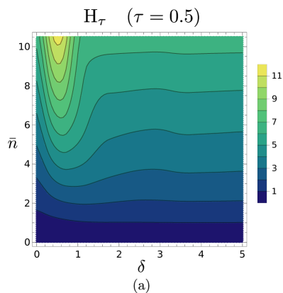
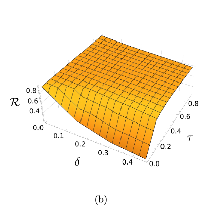
Figure 3: (a) Contour plot of the loss-QFI ${\rm H}_{\tau}$ for scenario ${\rm I}$, namely lossy-Kerr systems, as a function of the nonlinearity $\delta$ and the input energy $\bar{n}$ for $\tau=0.5$. For each $\bar{n}$ there exists a finite value $\delta_{\rm max}<\infty$ that maximizes the loss-QFI. (b) Plot of the quantumness ${\cal R}$ for scenario ${\rm I}$ as a function of the channel parameters $\tau$ and $\delta$ for an input energy $\bar{n}=1$. ${\cal R}$ is always nonzero and saturates in the limit of large $\tau$, proving the two parameters to be incompatible.

Finally, we assess the compatibility of the two parameters by computing the Uhlmann curvature $\boldsymbol{\cal U}$, equal to:

$$\boldsymbol{\cal U}=\left(\begin{array}[]{cc}0&{\cal U}_{\tau\delta}\\ -{\cal U}_{\tau\delta}&0\\ \end{array}\right)\,,$$ (19v)

where the off-diagonal term ${\cal U}_{\tau\delta}$ is computed from Equation (10) with the analogous method adopted for the QFIM. The numerical results show that ${\cal U}_{\tau\delta}$ is a decreasing function of $\tau$, being always nonzero for all $\tau$ and $\delta$. In turn, the two parameters cannot be jointly estimated with maximum precision. To quantify their incompatibility, we consider the quantumness ${\cal R}=\sqrt{\det\boldsymbol{\cal U}/\det{\bf H}}$, depicted in Figure 3(b). We have ${\cal R}>0$ and, in the limit of large $\tau$, ${\cal R}$ exhibits a weak dependence on $\delta$ and saturates. The saturation value is ${\cal R}_{\infty}\approx 0.8$ for $\bar{n}=1$ and increases for higher $\bar{n}$, suggesting the Holevo scalar bound introduced in Section 2 to be not close to the SLD-QFI bound.

3.2 Performance of feasible measurements

As we demonstrated above, the channel parameters $\tau$ and $\delta$ cannot be jointly estimated with maximum precision, thus the SLD-QCR bound is not attainable. Then, it becomes interesting to consider some feasible measurement schemes, that could be easily implemented in practice, and compare their performance with the ultimate bounds provided by the QFIM. Within this class, Gaussian measurements, such as homodyne and double-homodyne detection, provide the typical example of feasible detection strategies for optical signals [56]. In principle, photodetection could be also considered. Nevertheless, the photon-number distribution associated with state $\rho$ is retrieved from its diagonal matrix elements, namely $p(n|\boldsymbol{\lambda})=\langle n|\rho|n\rangle=\rho_{nn}$, being independent of the nonlinearity $\delta$, therefore the joint estimation problem is trivially reported to the single-parameter estimation of $\tau$.

To begin with, we compute the FIM ${\bf F}_{\rm h}$ associated with homodyne detection, corresponding to the measurement of the field quadrature:

$$\hat{x}_{\theta}=\sigma_{0}\left(ae^{-i\theta}+a^{\dagger}e^{i\theta}\right)\,,$$ (19w)

where $0\leq\theta<\pi$ determines the phase of the probed quadrature, and $\sigma_{0}^{2}$ is the shot-noise variance, corresponding to vacuum fluctuations, such that $\langle 0|\hat{x}_{\theta}^{2}|0\rangle=\sigma_{0}^{2}$[48]. We also remind that homodyne detection of $\hat{q}=\hat{x}_{0}=\sigma_{0}(a+a^{\dagger})$ provides the optimal measurement for the loss estimation in the absence of nonlinearity, saturating the single-parameter SLD-QCR bound [31], while it is only suboptimal for the nonlinearity estimation, due to the non-Gaussian nature of the Kerr effect. Performing detection of $\hat{x}_{\theta}$ is equivalent to the $1$-rank projective measurement $\Pi_{x}(\theta)=|x\rangle_{\theta}\langle x|$, where:

$$|x\rangle_{\theta}=\frac{e^{-x^{2}/2}}{\pi^{1/4}}\sum_{n=0}^{\infty}\frac{H_{n}(x)}{\sqrt{2^{n}n!}}\,e^{-in\theta}\,|n\rangle\,,$$ (19x)

$H_{n}(x)$ being the $n$-th Hermite polynomial [48]. In turn, the homodyne probability distribution reads

$$p_{\theta}(x|\boldsymbol{\lambda}) ={}_{\theta}\langle x|\rho|x\rangle_{\theta}$$ (19y)

$$=\frac{e^{-x^{2}}}{\sqrt{\pi}}\sum_{nm}\rho_{nm}\,\frac{H_{n}(x)H_{m}(x)}{\sqrt{2^{n+m}n!m!}}\,e^{i(n-m)\theta}\,,$$

and the corresponding FIM is numerically retrieved via Equation (3). In particular, we optimize the quadrature phase $\theta$ to achieve the maximum performance. Due to the incompatibility of $\tau$ and $\delta$, we identify three different cases:

• case (a): we optimize $\theta$ to maximize precision on the loss estimation, i.e. maximizing the loss-FI ${\rm F}_{{\rm h},\tau}={\rm F}_{{\rm h},\tau\tau}$;

• case (b): we optimize $\theta$ to maximize precision on the nonlinearity estimation, i.e. maximizing the nonlinearity-FI ${\rm F}_{{\rm h},\delta}={\rm F}_{{\rm h},\delta\delta}$;

• case (c): we optimize $\theta$ to maximize precision on the sum of the mean square errors for each parameter, i.e. maximizing ${\cal C}_{\rm h}=1/{\rm Tr}[{\bf F}_{{\rm h}}^{-1}]$, corresponding to minimize the inverse of trace of the inverse FIM.

Plots of ${\rm F}^{({\rm p})}_{{\rm h},\tau}$ and ${\rm F}^{({\rm p})}_{{\rm h},\delta}$, $\rm p=a,b,c$, as a function of the input energy $\bar{n}$ are depicted in Figure 4(a) and (b), respectively, compared to the corresponding QFIs. In both the cases, we see that, if properly optimized, the homodyne FI is close to the corresponding QFI for sufficiently small energy $\bar{n}$, while the separation increases for higher $\bar{n}$. With the chosen values of $\tau$ and $\delta$ we have ${\rm F}^{({\rm a})}_{{\rm h},\tau}\gtrsim 0.9\,{\rm H}_{\tau}$ for $\bar{n}\lesssim 2$, whereas ${\rm F}^{({\rm b})}_{{\rm h},\delta}\gtrsim 0.8\,{\rm H}_{\tau}$ for $\bar{n}\lesssim 4$. Moreover, we note that ${\rm F}^{({\rm c})}_{{\rm h},\tau}\approx{\rm F}^{({\rm a})}_{{\rm h},\tau}$, while the three subcases lead to distinct FIs for the nonlinearity estimation. The plots of the optimized phase $\theta_{\rm max}^{({\rm p})}$, $\rm p=a,b,c$, are depicted in Figure 5, where the jump that appears is only consequence of the $\pi$-periodicity of the phase, which, by construction, has been constrained in the interval $0\leq\theta<\pi$. Given this consideration, both $\theta_{\rm max}^{(\rm a)}$ and $\theta_{\rm max}^{(\rm c)}$ are decreasing function of $\bar{n}$. On the contrary, in case (b), the optimized phase is non-monotonic: it is $\theta_{\rm max}^{({\rm b})}\approx\pi/2$ for $\bar{n}\ll 1$, while it drops to $0$ for $\bar{n}\geq\bar{n}_{0}$, showing quadrature $\hat{q}$ to be the best one for the nonlinearity estimation. The discontinuity in the derivative of $\theta_{\rm max}^{({\rm b})}$ at $\bar{n}_{0}$ is then reflected in the cusp of ${\rm F}^{({\rm b})}_{{\rm h},\tau}$, see Figure 4(a).

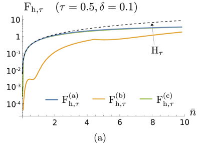
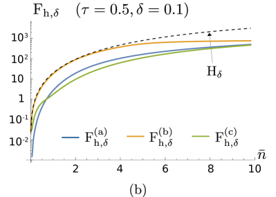
Figure 4: Log plot of the loss-FI ${\rm F}^{({\rm p})}_{{\rm h},\tau}$ for homodyne detection under scenario ${\rm I}$, namely lossy-Kerr systems, (a) and the nonlinearity-FI ${\rm F}^{({\rm p})}_{{\rm h},\delta}$ (b), $\rm p=a,b,c$, as a function of $\bar{n}$. Homodyne detection proves itself to be nearly optimal for both loss and nonlinearity estimation in the low-energy regime. We set the values $\tau=0.5$ and $\delta=0.1$ for the loss and nonlinearity parameters, respectively.

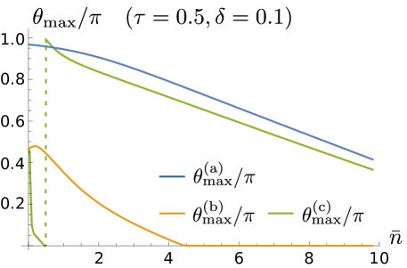
Figure 5: Plot of the optimized quadrature phases $\theta_{\rm max}^{({\rm p})}/\pi$, $\rm p=a,b,c$, for homodyne detection under scenario ${\rm I}$, namely lossy-Kerr systems, as a function of $\bar{n}$. We set the values $\tau=0.5$ and $\delta=0.1$ for the loss and nonlinearity parameters, respectively.

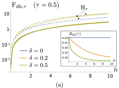
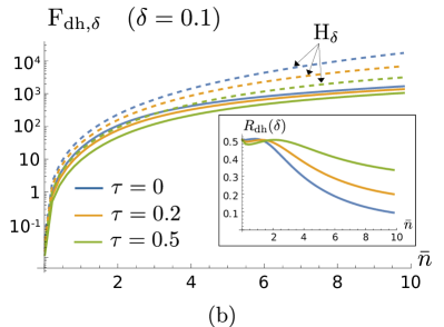
Figure 6: (a) Log plot of the loss-FI ${\rm F}_{{\rm dh},\tau}$ for DH detection under scenario ${\rm I}$, namely lossy-Kerr systems, and plot of the relative ratio $R_{\rm dh}(\tau)={\rm F}_{{\rm dh},\tau}/{\rm H}_{\tau}$ (in the inset) as a function of $\bar{n}$ for $\tau=0.5$ and different values of the nonlinearity $\delta$. (b) Log plot of the nonlinearity-FI ${\rm F}_{{\rm dh},\delta}$ and plot of the relative ratio $R_{\rm dh}(\delta)={\rm F}_{{\rm dh},\delta}/{\rm H}_{\delta}$ (in the inset) as a function of $\bar{n}$ for $\delta=0.1$ and different values of the loss parameter $\tau$.

Now, we address the second example of feasible POVM, that is double-homodyne (DH) detection. It corresponds to joint measurement of the two orthogonal quadratures, obtained by splitting the incoming signal in two copies at a balanced beam splitter and then homodyning $\hat{q}=\hat{x}_{0}$ and $\hat{p}=\hat{x}_{\pi/2}$ on the transmitted and reflected branch, retrieving a pair of real outcomes $(x,y)\in\mathbb{R}^{2}$, respectively. The main consequence of the signal splitting is the introduction of a ineludible excess noise on both the output quadrature statistics, equal to $\sigma_{0}^{2}$, that guarantees joint measurement without violation of the Heisenberg’s uncertainty principle [55]. This excess noise makes DH only suboptimal for the loss estimation in the absence of nonlinearity, its associated FI being exactly one half of the QFI achieved by single-homodyne of $\hat{q}$ [31]. Equivalently, DH detection is described as a $1$-rank (non-orthogonal) projection on coherent states, with associated POVM $\Pi_{x,y}=|\zeta_{x,y}\rangle\langle\zeta_{x,y}|/2\pi$, where $|\zeta_{x,y}\rangle$ is a coherent state with amplitude $\zeta_{x,y}=(x+iy)/\sqrt{2}$, such that $\int dxdy\,\Pi_{x,y}=\hat{{\mathbbm{1}}}$. In turn, the corresponding probability distribution given state $\rho$ reads:

$$p_{\rm dh}(x,y|\boldsymbol{\lambda}) =\frac{1}{2\pi}\langle\zeta_{x,y}|\rho|\zeta_{x,y}\rangle$$ (19z)

$$=\frac{e^{-(x^{2}+y^{2})/2}}{2\pi}\sum_{nm}\frac{\rho_{nm}}{\sqrt{n!m!}}\left(\frac{x-iy}{\sqrt{2}}\right)^{n}\left(\frac{x+iy}{\sqrt{2}}\right)^{m}\,,$$

from which we compute the FIM ${\bf F}_{\rm dh}=({\rm F}_{{\rm dh},\mu\nu})_{\mu,\nu}$ thanks to (3). Figure 6(a) and (b) shows the resulting FIM elements ${\rm F}_{{\rm dh},\tau}$ and ${\rm F}_{{\rm dh},\delta}$, respectively, as a function of the input energy $\bar{n}$. As we can see, DH detection is weakly dependent on the nonlinearity $\delta$, as the value of ${\rm F}_{{\rm dh},\tau}$ is almost the same for different $\delta$, whereas it proves itself quite robust against the loss, since ${\rm F}_{{\rm dh},\delta}$ decreases more slowly than ${\rm H}_{\delta}$ when $\tau$ is increased. To better enlighten these effects, we consider the relative ratios:

$$R_{\rm dh}(\mu)=\frac{{\rm F}_{{\rm dh},\mu}}{{\rm H}_{\mu}}\,,\quad\mu=\tau,\delta\,,$$ (19aa)

depicted in the insets of Figure 6. As regards the loss estimation, if $\delta=0$, we have $R_{\rm dh}(\tau)=0.5$, retrieving the known result for single-parameter estimation, whereas for $\delta>0$ the ratio decreases, since the loss-QFI is enhanced while the FI value ${\rm F}_{{\rm dh},\tau}$ remains almost stable. On the contrary, in estimating the Kerr nonlinearity we identify two different regimes. If $\bar{n}\ll 1$, $R_{\rm dh}(\delta)$ decreases with $\tau$, while, on the other hand, for high enough energy the situation is reversed and $R_{\rm dh}(\delta)$ gets higher values for larger losses, showing higher robustness against decoherence. Beside this, DH is always suboptimal, and the ratio $R_{\rm dh}(\mu)$, $\tau,\delta$ is lower than $0.5$ in all conditions.

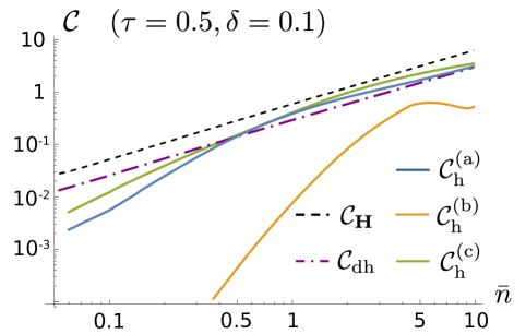
Figure 7: Log-log plot of the trace scalar bounds for scenario I, namely lossy-Kerr systems, that is the SLD-QFIM bound ${\cal C}_{\bf H}=1/{\rm Tr}[{\bf H}^{-1}]$, and the FIM bounds for homodyne detection, ${\cal C}^{({\rm p})}_{\rm h}=1/{\rm Tr}[({\bf F}_{\rm h}^{({\rm p})})^{-1}]$, $\rm p=a,b,c$, and DH detection, ${\cal C}_{\rm dh}=1/{\rm Tr}[{\bf F}_{\rm dh}^{-1}]$, as a function of $\bar{n}$. We set the values $\tau=0.5$ and $\delta=0.1$ for the loss and nonlinearity parameters, respectively.

To conclude, we also compare the performance of the previous measurement schemes in terms of scalar Cramér-Rao bounds. In particular, we choose the weight matrix ${\bf W}={\mathbbm{1}}_{2}$, ${\mathbbm{1}}_{2}$ being the $2\times 2$ identity matrix, in which case the figure of merit is the trace of the inverse FIMs. Then, the covariance matrix $\bf V$ of an unbiased estimator satisfies ${\rm Tr}[{\bf V}]\geq 1/{\cal C}\geq 1/{\cal C}_{\bf H}$, with ${\cal C}^{({\rm p})}_{{\rm h}}=1/{\rm Tr}[({\bf F}^{({\rm p})}_{\rm h})^{-1}]$, $\rm p=a,b,c$, for homodyne detection, ${\cal C}_{{\rm dh}}=1/{\rm Tr}[{\bf F}_{\rm dh}^{-1}]$ for DH detection, and ${\cal C}_{\bf H}=1/{\rm Tr}[{\bf H}^{-1}]$, in which, for the sake of simplicity, we set the number of measurements equal to $M=1$. Plots of the trace scalar bounds are reported in Figure 7. Consistently with the former results, none of the considered measurements is able to reach ${\cal C}_{\bf H}$. Nevertheless, as we can see, homodyne detection for case (c), is nearly optimal for a sufficiently high input energy, being beaten by DH detection only in the low-energy limit $\bar{n}\ll 1$, when ${\cal C}_{{\rm dh}}\geq{\cal C}^{({\rm c})}_{{\rm h}}$. Remarkably, the performance of case (a) is close to (c), whilst case (b) is strongly suboptimal. This is mainly due to the different sensitivity to $\tau$ and $\delta$ of the off diagonal element of matrix ${\bf F}_{{\rm h}}$. Finally, in the limit of high $\bar{n}$, DH detection approaches case (a)-homodyne detection, as ${\cal C}_{{\rm dh}}\approx{\cal C}^{({\rm a})}_{{\rm h}}$, proving itself as a versatile solution, that does not involve optimization of the experimental setup, in all energy regimes, regardless its suboptimality.

4 Scenario II: Joint estimation of dephasing and Kerr nonlinearity

We now move on to the second scenario under investigation, and perform characterization of noisy systems in the presence of Kerr nonlinearity and dephasing produced by phase diffusion [57, 58]. This is a typical situation emerging in quantum optomechanical systems, consisting in an optical cavity whose mirrors experience quantized vibrations at acoustic frequencies. The mechanical oscillations of the mirrors, then, induce a change in the effective length of the cavity and, accordingly, in its proper frequency, resulting in an overall interaction between the corresponding optical and mechanical bosonic modes [34]. In particular, if the acoustic modes are excited in a thermal state, the reduced dynamics of the optical cavity field is equivalent to a phase diffusion master equation with an effective self-Kerr unitary interaction, where both the noise and nonlinearity parameter depend on the strength of the optomechanical interaction [35]. That is, the evolution of the optical state $\rho$ of the cavity field follows:

$$\frac{d\rho}{dt}=-i\left[\hat{H}_{\kappa},\rho\,\right]+\gamma\,{\cal L}[a^{\dagger}a]\,\rho\,,$$ (19ab)

with the $\hat{H}_{\kappa}$ in Equation (14) and $\kappa$ and $\gamma$ being the effective Kerr coupling and phase diffusion rates, respectively. The solution to the master equation at time $t$, $\rho=\rho(t)$, is straightforwardly obtained by expanding $\rho$ on the Fock basis, namely $\rho=\sum_{nm}\rho_{nm}|n\rangle\langle m|$, leading to:

$$\rho_{nm}=\frac{\alpha^{n}\left(\alpha^{*}\right)^{m}}{\sqrt{n!m!}}\exp\left\{-|\alpha|^{2}-i\delta(n^{2}-m^{2})-\frac{\sigma^{2}}{2}(n-m)^{2}\right\}\,,$$ (19ac)

with the coherent state $|\alpha\rangle$ as input, and where:

$$\sigma=\sqrt{\gamma t}\qquad\mbox{and}\qquad\delta=\kappa t\,,$$ (19ad)

represent the dephasing parameter, also referred to as phase noise amplitude, and the nonlinearity parameter, respectively. Differently from scenario ${\rm I}$, both the Hamiltonian and Lindblad dynamics are generated by the photon-number operator, thus solution (19ac) can be re-expressed as:

$$\rho=e^{-i\delta(a^{\dagger}a)^{2}}\,\varrho_{\sigma}\,e^{-i\delta(a^{\dagger}a)^{2}}\,,$$ (19ae)

$\varrho_{\sigma}=e^{-|\alpha|^{2}}\sum_{nm}e^{-\sigma^{2}(n-m)^{2}/2}\,\alpha^{n}(\alpha^{*})^{m}/\sqrt{n!m!}$ being a dephased coherent state, namely as the subsequent application of a dephasing completely-positive map followed a unitary Kerr evolution. In turn, now, no pure-state approximation can be carried out, since the presence of phase diffusion makes $\rho$ mixed for all $\sigma>0$. The stationary state of the dynamics, achieved in the limits $\sigma\gg 1$ and $\delta\gg 1$, is the phase-averaged (PHAV) state [59]:

$$\rho_{\rm PHAV}=e^{-|\alpha|^{2}}\sum_{n}\frac{|\alpha|^{2n}}{n!}\,|n\rangle\langle n|\,,$$ (19af)

corresponding to a Poisson-distributed ensemble of Fock states, being insensitive to the nonlinearity. In this scenario, we have a statistical model $\rho$ encoding parameters $\boldsymbol{\lambda}=(\sigma,\delta)$. As before, we compute the QFIM and the Uhlmann curvature, to assess the ultimate precision limits. Then, we further compute the FIM associated with homodyne and DH detection, comparing their performances to the SLD-QCR bound.

4.1 Computation of the QFIM

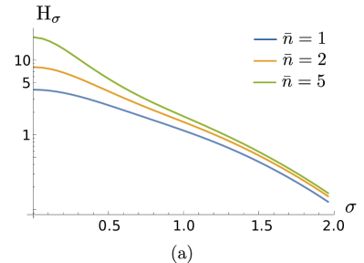
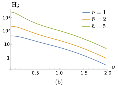
Figure 8: Log plots of the dephasing-QFI ${\rm H}_{\sigma}$ (a) and nonlinearity-QFI ${\rm H}_{\delta}$ (b) for scenario ${\rm II}$, namely dephasing-Kerr systems, as a function of the phase noise parameter $\sigma=\sqrt{\gamma t}$ for different input coherent state energy $\bar{n}=|\alpha|^{2}$. Both the QFIs are decreasing functions of the noise $\sigma$, being independent of the nonlinearity parameter $\delta=\kappa t$.

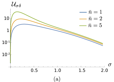
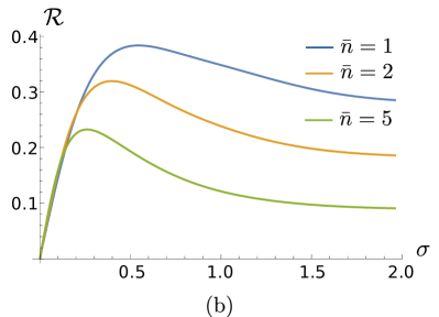
Figure 9: (a) Log plot of the Uhlmann quadrature ${\cal U}_{\sigma\delta}$ for scenario ${\rm II}$, namely dephasing-Kerr systems, as a function of the phase noise parameter $\sigma=\sqrt{\gamma t}$ for different input coherent state energy $\bar{n}=|\alpha|^{2}$. (b) Plot of the quantumness ${\cal R}$ for scenario ${\rm II}$ as a function of $\sigma$ for different $\bar{n}$. Both the quantities are independent of the nonlinearity parameter $\delta=\kappa t$. In particular, ${\cal R}$ is a non-monotonous function of $\sigma$, saturating in the large-noise regime to ${\cal R}_{\infty}>0$, proving the two parameters to be incompatible.

We numerically compute the QFIM ${\bf H}=({\rm H}_{\mu\nu})_{\mu,\nu}$, $\mu,\nu=\sigma,\delta$, by Equation (6), where $\partial_{\mu}\rho=\sum_{nm}(\partial_{\mu}\rho_{nm})|n\rangle\langle m|$, $\mu=\tau,\delta$. We note that, thanks to the structure of the encoded state, see Equation (19ae), the statistical model is covariant with respect to the nonlinearity, and the corresponding QFIM turns out to be independent of $\delta$ [45]. Furthermore, differently from scenario ${\rm I}$, now the QFIM is a diagonal matrix, that is ${\rm H}_{\sigma\delta}=0$, and its diagonal elements ${\rm H}_{\sigma}={\rm H}_{\sigma\sigma}$ and ${\rm H}_{\delta}={\rm H}_{\delta\delta}$, reported in Figure 8(a) and (b), respectively, are decreasing with the dephasing parameter $\sigma$. In particular, the presence of Kerr susceptibility is irrelevant for the dephasing estimation, as $H_{\sigma}$ is a function of the sole noise $\sigma$ and input energy $\bar{n}=|\alpha|^{2}$, in contrast to the case of loss estimation. To assess compatibility, we consider the Uhlmann curvature $\boldsymbol{\cal U}$, being an off-diagonal matrix as in (19v), to be computed thanks to (10). The behaviour is different with respect to scenario ${\rm I}$. In fact, the off-diagonal term ${\cal U}_{\sigma\delta}$, depicted in Figure 9(a), is a non-monotonous function of $\sigma$, reaching a maximum at a finite noise $\sigma_{\rm max}$ and, thereafter, decreasing towards $0$. Moreover, like the QFIM, it increases with the signal energy $\bar{n}$, being independent of $\delta$. The non-monotonicity of the Uhlmann quadrature is reflected on the quantumness ${\cal R}=\sqrt{\det\boldsymbol{\cal U}/\det{\bf H}}$, plotted in Figure 9(b). For low noise, ${\cal R}$ increases with $\sigma$ until to reach a maximum, after which it decreases, saturating for $\sigma\gg 1$ to an asymptotic value ${\cal R}_{\infty}>0$. The saturation value is lower for increasing energy, whilst the situation is reversed in the low-noise regime, where higher $\bar{n}$ makes $\cal R$ increase. As a consequence, even in this scenario, the two parameters are not compatible, and cannot be jointly estimated without the addition of an excess noise.

4.2 Performance of feasible measurements

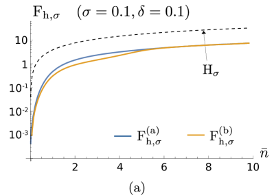
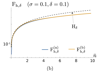
Figure 10: Log plot of the dephasing-FI ${\rm F}^{({\rm p})}_{{\rm h},\sigma}$ (a) and the nonlinearity-FI ${\rm F}^{({\rm p})}_{{\rm h},\delta}$ (b), $\rm p=a,b$, for scenario ${\rm II}$, namely dephasing-Kerr systems, as a function of $\bar{n}$. Numerical calculations show that case (c) is almost indistinguishable from case (a). Differently from the lossy-Kerr scenario, now, homodyne detection is strongly suboptimal for the noise estimation, whilst being nearly optimal for the nonlinearity estimation. We set the values $\sigma=0.1$ and $\delta=0.1$ for the dephasing and nonlinearity parameter, respectively.

As before, we now quantify the performance of homodyne and DH detection in the joint estimation of $\sigma$ and $\delta$. Differently from scenario ${\rm I}$, the physical process associated with phase noise derives from non-Gaussian interaction, therefore we expect Gaussian measurement to be suboptimal even in the limit case $\delta=0$ [60, 61]. The homodyne probability $p_{\theta}(x|\boldsymbol{\lambda})$ is retrieved from Equation (19y), from which we compute the FIM ${\bf F}_{\rm h}=({\rm F}_{{\rm h},\mu\nu})_{\mu,\nu}$. As before, we identify the three cases in which we optimize the phase of the measured quadrature to maximize the noise-FI ${\rm F}_{{\rm h},\sigma}={\rm F}_{{\rm h},\sigma\sigma}$ (a), to maximize the nonlinearity-FI ${\rm F}_{{\rm h},\delta}={\rm F}_{{\rm h},\delta\delta}$ (b), and to maximize the trace scalar bound ${\cal C}_{\rm h}=1/{\rm Tr}[({\bf F}_{{\rm h}})^{-1}]$ (c), respectively. Plots of ${\rm F}^{({\rm p})}_{{\rm h},\sigma}$ and ${\rm F}^{({\rm p})}_{{\rm h},\delta}$, $\rm p=a,b$, as a function of the input energy $\bar{n}$ are depicted in Figure 10(a) and (b), respectively compared to the corresponding QFIs. Numerical calculations show that case (c) is almost indistinguishable from case (a), therefore we do not explicitly report it in the following Figures. ${\rm F}^{({\rm a})}_{{\rm h},\sigma}$ is monotonously increasing with $\bar{n}$, but the separation with respect to ${\rm H}_{\sigma}$ is large, as ${\rm F}^{({\rm a})}_{{\rm h},\sigma}<0.25{\rm H}_{\sigma}$ for all $\bar{n}$, proving homodyne detection to be strongly suboptimal for the noise estimation. On the contrary, the estimation of Kerr nonlinearity is qualitatively similar to that in Section 3.2: we have ${\rm F}^{({\rm b})}_{{\rm h},\delta}\gtrsim 0.8{\rm H}_{\delta}$ for $\bar{n}\lesssim 2.25$, and the homodyne is nearly optimal in the low-energy limit. However, in both the cases, the performances of cases (a) and (b) are close with each other, and almost coincide in the high-energy regime. The optimized phase $\theta_{\rm max}^{({\rm p})}$, $\rm p=a,b$, is depicted in Figure 11, showing a similar behaviour for cases (a) and (b), while the phase jumps are again consequence of the $\pi$-periodicity.

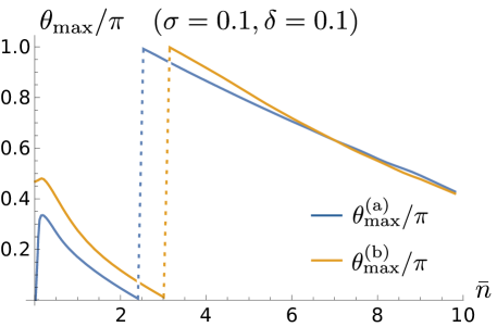
Figure 11: Plot of the optimized quadrature phases $\theta_{\rm max}^{({\rm p})}/\pi$, $\rm p=a,b$, for homodyne detection under scenario ${\rm II}$, namely dephasing-Kerr systems, as a function of $\bar{n}$. Numerical calculations show that case (c) is almost indistinguishable from case (a). We set the values $\sigma=0.1$ and $\delta=0.1$ for the dephasing and nonlinearity parameter, respectively.

Moving to the case of DH detection, we compute the probability $p_{\rm dh}(x,y|\boldsymbol{\lambda})$ from Equation (19z), and its corresponding FIM ${\bf F}_{\rm dh}=({\rm F}_{{\rm dh},\mu\nu})_{\mu,\nu}$. The resulting elements ${\rm F}_{{\rm dh},\sigma}$ and ${\rm F}_{{\rm dh},\delta}$ are plotted in Figure 12(a) and (b), respectively. As regards the noise estimation, we see that DH detection is strongly suboptimal and, in particular, worse than single homodyne detection, since ${\rm F}_{{\rm dh},\sigma}<0.2{\rm H}_{\sigma}$. However, the dependence of ${\rm F}_{{\rm dh},\sigma}$ on the nonlinearity is nontrivial, as, in the low-energy regime, the noise-FI is enhanced by increasing $\delta$. Instead, the behaviour of the nonlinearity-FI is similar to that in Section 3.2, that is, DH is suboptimal but ${\rm F}_{{\rm dh},\delta}$ is quite robust against the noise, differently than the corresponding QFI, such that the relative ratio $R_{\rm dh}(\delta)={\rm F}_{{\rm dh},\delta}/{\rm H}_{\delta}$ is increased for larger noise in the high-energy limit.

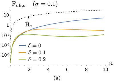
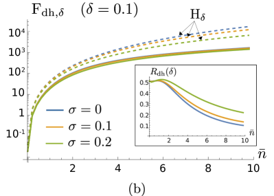
Figure 12: (a) Log plot of the dephasing-FI ${\rm F}_{{\rm dh},\sigma}$ for scenario ${\rm II}$, namely dephasing-Kerr systems, as a function of $\bar{n}$ for the dephasing parameter $\sigma=0.1$ and different values of the nonlinearity $\delta$. (b) Log plot of the nonlinearity-FI ${\rm F}_{{\rm dh},\delta}$ and plot of the relative ratio $R_{\rm dh}(\delta)={\rm F}_{{\rm dh},\delta}/{\rm H}_{\delta}$ (in the inset) for scenario ${\rm II}$ as a function of $\bar{n}$ for nonlinearity $\delta=0.1$ and different values of the dephasing $\sigma$.

Finally, we consider the trace of the inverse FIM matrices as an example of scalar Cramér-Rao bound, depicted in Figure 13. That is, we compute the quantities ${\cal C}^{({\rm p})}_{{\rm h}}=1/{\rm Tr}[({\bf F}^{({\rm p})}_{\rm h})^{-1}]$, $\rm p=a,b$, ${\cal C}_{{\rm dh}}=1/{\rm Tr}[{\bf F}_{\rm dh}^{-1}]$, and ${\cal C}_{\bf H}=1/{\rm Tr}[{\bf H}^{-1}]$, with the choice of $M=1$ measurements. As we can see, homodyne detection, in both cases $\rm p=a,b$, is nearly optimal and, differently from scenario ${\rm I}$, significantly outperforms DH detection for sufficiently high energy. This suggests that probing a single quadrature with optimized phase is worth of implementation in order to achieve a closer performance to the SLD-QFI limit.

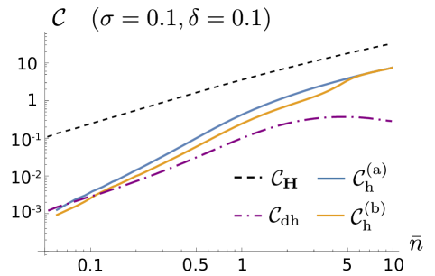
Figure 13: Log-log plot of the trace scalar bounds for scenario ${\rm II}$, namely dephasing-Kerr systems, that is the SLD-QFIM bound ${\cal C}_{\bf H}=1/{\rm Tr}[{\bf H}^{-1}]$, and the FIM bounds for homodyne detection, ${\cal C}^{({\rm p})}_{\rm h}=1/{\rm Tr}[({\bf F}_{\rm h}^{({\rm p})})^{-1}]$, $\rm p=a,b$, and DH detection, ${\cal C}_{\rm dh}=1/{\rm Tr}[{\bf F}_{\rm dh}^{-1}]$, as a function of $\bar{n}$. Numerical calculations show that case (c) is almost indistinguishable from case (a). We set the values $\sigma=0.1$ and $\delta=0.1$ for the dephasing and nonlinearity parameter, respectively.

5 Discussion

The results obtained in the paper show some relevant qualitative differences between the two scenarios under investigation. In fact, if the behaviour of the nonlinearity estimation is similar in both the scenarios, i.e. decoherence detriments the QFI ${\rm H}_{\delta}$, two opposite situations arise for the decoherence estimation, since the presence of Kerr nonlinearity enhances the loss-QFI ${\rm H}_{\tau}$, while it does not affect the dephasing-QFI ${\rm H}_{\sigma}$. These considerations raise the question of identifying a proper resource, connected to a quantum property of the encoded states, being somehow responsible for the presence of absence of a QFI enhancement in one scenario or another. This would provide a fundamental interpretation of our results, fostering new methods for engineering more sensitive probe states and measurement schemes.

In light of this, non-Gaussianity has been firstly proposed as a suitable candidate [29, 31], which can be quantified by the difference between the von-Neumann entropy ${\sf S}[\rho]=-{\rm Tr}[\rho\log\rho]$ of a quantum state $\rho$ and that of its associated Gaussian state $\rho_{\rm G}$, sharing the same first moment vector and covariance matrix, i.e. ${\cal N}[\rho]={\sf S}[\rho_{\rm G}]-{\sf S}[\rho]$ [62, 63]. In fact, in scenario ${\rm I}$, namely lossy-Kerr systems, the presence of a nonzero Kerr susceptibility turns a Gaussian statistical model into a non-Gaussian and non-classical one during the evolution. However, the stationary state of the dynamics is the vacuum state, which is Gaussian, therefore the resulting ${\cal N}[\rho]$ would be a non monotonous function of $\tau$, increasing in the limit $\tau\ll 1$ and then decreasing towards $0$ for $\tau\gg 1$, thus qualitatively reproducing the results in Figures 1(a) and 2(a). Nevertheless, we did not find a quantitative correspondence between the QFI and the non-Gaussianity, as, in general, the states leading to the highest increase in the loss-QFI ${\rm H}_{\tau}$ are not the one with the highest ${\cal N}[\rho]$. Furthermore, the previous argument fails when applied to scenario ${\rm II}$, namely dephasing-Kerr systems, where both phase diffusion and Kerr interaction are non-Gaussian, and ${\cal N}[\rho]$ is an increasing function of both $\sigma$ and $\delta$, whilst ${\rm H}_{\sigma}$ is insensitive to the nonlinearity. We reach a similar conclusion by also claiming non-classicality as a resource, described in terms of Wigner negativity and measured, for instance, by the quadrature coherence scale (QCS) [64, 65, 66, 67]. Indeed, in both the scenarios, the initial and stationary states are classical, therefore we expect the QCS to be non monotonous with $\delta$, which, again, would not reproduce the behaviour of ${\rm H}_{\sigma}$.

On the other hand, starting from the results of scenario ${\rm II}$, we may propose as resource the coherence of the quantum statistical model [68, 69, 70, 71]. In particular, a measure of coherence for a quantum state $\rho$ in a given basis $\{|\varphi_{j}\rangle\}_{j}$ has been introduced by Baumgratz et al. in [68], and reads ${\sf C}[\rho]=\sum_{j\neq k}|\rho_{jk}|$, with $\rho_{jk}=\langle\varphi_{j}|\rho|\varphi_{k}\rangle$. This captures the behaviour of ${\rm H}_{\sigma}$ in scenario ${\rm II}$, since the presence of Kerr nonlinearity only appears as a phase in the Fock state expansion of $\rho$, thus not changing its coherence in the Fock basis. However, in scenario ${\rm I}$, numerical calculations show that nonlinearity reduces the coherence ${\sf C}[\rho]$ with respect to the case $\delta=0$, whilst increasing ${\rm H}_{\tau}$.

In summary, for scenario ${\rm I}$, namely lossy-Kerr systems, we should conclude that non-Gaussianity in itself (as well as non-classicality) is a necessary but not sufficient condition to enhance the QFI with respect to the performance of coherent probes, since there is no monotonous relation between ${\cal N}[\rho]$ and ${\rm H}_{\tau}$. We note that this conclusion can be further extended to all Gaussian probes, according to recent results derived in [31, 72, 73]. Instead, in scenario ${\rm II}$, namely dephasing-Kerr systems, quantum coherence seems to be a reasonably necessary condition to improve the precision of dephasing estimation, but we have no evidence that states with higher coherence enhance ${\rm H}_{\delta}$. In both the scenarios, none of the previous figures of merit provide a complete understanding of the sensitivity of the statistical model to the encoded parameters, therefore raising the interesting problem of the resource identification.

Table 1: Summary of the results obtained from the QFIM analysis in the two scenarios under investigation, corresponding to loss-Kerr and dephasing-Kerr systems, respectively.

	Noise estimation	Nonlinearity estimation	Compatibility
Scenario I	enhancement	reduction	no
(lossy-Kerr)
Scenario II	no enhancement	reduction	no
(dephasing-Kerr)

Table 2: Summary of the results obtained from the FIM analysis in the two scenarios under investigation, corresponding to loss-Kerr and dephasing-Kerr systems, respectively.

		Homodyne detection			Double
					homodyne
		(a)	(b)	(c)	detection
	Loss	nearly	strongly	suboptimal	suboptimal
	estimation	optimal	suboptimal
Scenario I	Nonlinearity	suboptimal	nearly	suboptimal	suboptimal
(lossy-Kerr)	estimation		optimal
	Scalar bound	suboptimal	strongly	suboptimal	suboptimal
			suboptimal
	Dephasing	strongly	strongly	strongly	strongly
	estimation	suboptimal	suboptimal	suboptimal	suboptimal
Scenario II	Nonlinearity	suboptimal	nearly	suboptimal	suboptimal
(dephasing-Kerr)	estimation		optimal
	Scalar bound	suboptimal	suboptimal	suboptimal	strongly
					suboptimal

6 Conclusions

In this paper, we have addressed characterization of noisy Kerr channels, in the presence of either loss or dephasing and a nonzero self-Kerr interaction, by considering a coherent state as a probe. In both the scenarios, we have addressed the joint estimation of the decoherence and nonlinearity parameters in terms of the QFIM, that provides the ultimate bound to the covariance matrix of any unbiased estimator. In lossy-Kerr systems, we showed that the presence of nonlinearity enhances the loss-QFI ${\rm H}_{\tau}$ in the regime of small loss parameter $\tau$, corresponding to low loss rate of the optical medium or short-distance transmission, and low input energy $\bar{n}$. In particular, we proved that, for any $\bar{n}$, there exists a finite value $\delta_{\rm max}$ of the nonlinearity that maximizes ${\rm H}_{\tau}$, whereas the presence of loss always reduces the QFI for the nonlinearity. Moreover, the Uhlmann curvature is nonzero, thus the two parameters are not compatible and cannot be jointly estimated with maximum precision. On the other hand, in dephasing-Kerr systems, both the dephasing and nonlinearity QFIs are independent of the nonlinearity parameter $\delta$ and decreasing with the noise amplitude $\sigma$, therefore no enhancement is observed. The Uhlmann quadrature is still nonzero, so the two parameters are incompatible too. A summary of these results is reported in Table 1.

Thereafter, we considered some relevant examples of feasible POVMs, i.e. homodyne detection and DH detection, and compute the corresponding FIM, to assess their performance with respect to the ultimate bound provided by the QFIM. Table 2 reports a comprehensive sum-up of all the obtained results. In the presence of lossy-Kerr systems, homodyne detection of a suitably optimized quadrature provides a nearly optimal performance in the low-energy regime, close to the SLD-QCR bound, while DH detection provides a suboptimal solution, although being robust against losses. Instead, in the dephasing-Kerr scenario, homodyne detection remains nearly optimal only for the nonlinearity estimation, whereas the noise-FI is significantly lower than the corresponding QFI ${\rm H}_{\sigma}$. Similarly, DH detection is strongly suboptimal for the dephasing estimation, whereas it shows robustness also against phase noise in the estimation of the nonlinearity. Finally, we evaluated a trace scalar bound, proving DH and optimized homodyne detection to be suboptimal in the low- and high- energy regimes, respectively. In particular, in scenario ${\rm I}$, namely lossy-Kerr systems, DH measurement is closer to homodyne, proving itself as a versatile solution in all conditions.

The obtained results offer a qualitative comparison between the two scenarios and quantify the impact of nonlinearity, being non-negligible in many platforms, for characterization of quantum channels. In particular, they provide a starting point for practical implementations in quantum information protocols, such as sensing [74], quantum communications [75] and quantum key distribution [76].

References

References

- [1] Dell’Anno F, De Siena S, and Illuminati F, 2006 Phys. Rep. 428 53–168
- [2] Chang D, Vuletić V, and Lukin M 2014 Nat. Photonics 8 685–694
- [3] Chekhova M V and Ou Z Y 2016 Adv. Opt. Photon. 8 104–155
- [4] Combes J and Brod D J 2018 Phys. Rev. A 98 062313
- [5] Candeloro A, Razavian S, Piccolini M, Teklu B, Olivares S, and Paris M G A 2021 Entropy 23 1353
- [6] Takatsuji M 1967 Phys. Rev. 155 980
- [7] Milburn G J and Holmes C A 1986 Phys. Rev. Lett. 56 2237
- [8] Stobińska M, Milburn G J, and Wódkiewicz K 2008 Phys. Rev. A 78 013810
- [9] Yurke B and Stoler D 1986 Phys. Rev. Lett. 57 13
- [10] Yurke B and Stoler D 1988 Physica B 151 298
- [11] Miranowicz A, Tanas R, and Kielich S 1990 Quantum Opt. 2 253
- [12] Paris M G A 1999 J. Opt. B: Quantum Semiclass. Opt. 1 662–667
- [13] Jeong H, Kim M S, Ralph T C, and Ham B S 2004 Phys. Rev. A 70 061801
- [14] Sizmann A and Leuchs G 1999 Prog. Optics 39 373–469
- [15] Hau L V, Harris S E, Dutton Z, and Behroozi C H 1999 Nature 397 594–598
- [16] Kang H and Zhu Y 2003 Phys. Rev. Lett. 91 093601
- [17] Yin Y et al. 2012 Phys. Rev. A 85 023826
- [18] Al-Nashy B, Amin S M M, and Al-Khursan A H 2014 J. Opt. Soc. Am. B 31 1991–1996
- [19] Zhang H and Wang H 2017 Phys. Rev. A 95 052314
- [20] Zhang Z, Scully M O, and Agarwal G S 2019 Phys. Rev. Research 1 02302
- [21] Yang Z-B et al. 2022 Phys. Rev. A 106 012419
- [22] Boyd R 2008 Nonlinear Optics, 3rd ed. (Academic Press, Burlington, MA)
- [23] Kunz L, Paris M G A, and Banaszek K 2018 J. Opt. Soc. Am. B 35 214–222
- [24] Mitra P P and Stark J B 2001 Nature 411 1027–1030
- [25] Wegener L, Povinelli M, Green A, Mitra P, Stark J B, and Littlewood P 2004 Physica D 189 81–99
- [26] Ellis A, Zhao J, and Cotter D 2010 J. Lightwave Technol. 28 423–433
- [27] R.-J. Essiambre R-J and Tkach R W 2012 Proc. IEEE 100 1035
- [28] Temprana E, Myslivets E, Kuo B-P, Liu L, Ataie V, Alic N, and Radic S 2015 Science 348 1445–1448
- [29] Genoni M G, Invernizzi C, and Paris M G A 2009 Phys. Rev. A 80 033842
- [30] Luis A and Rivas Á 2015 Phys. Rev. A 92 022104
- [31] Rossi M, Albarelli F, and Paris M G A 2016 Phys. Rev. A 93 053805
- [32] Zidan N, Abdel-Hameed H F, and Metwally N 2019 Sci. Rep. 9 2699
- [33] Aspelmeyer M, Kippenberg T J, and Marquardt F 2014 Rev. Mod. Phys. 86 1391
- [34] Bowen W P and Milburn G J 2015 Quantum Optomechanics (CRC Press, Boca Raton)
- [35] Xu Q and Blencowe M P2014 2021 Phys. Rev. A 104 063509
- [36] Helstrom C W 1976 Quantum Detection and Estimation Theory (Elsevier Academic Press)
- [37] Razavian S, Paris M G A, and Genoni M G 2020 Entropy 22 1197
- [38] Albarelli F, Barbieri M, Genoni M G, and Gianani I 2020 Phys. Lett. A 384 126311
- [39] Asjad M, Teklu B, and Paris M G A 2023 Phys. Rev. Research 5 013185
- [40] Helstrom C W 1967 Phys. Lett. A 25 101
- [41] Yuen H P and Lax M 1973 IEEE Trans. Inf. Theory 19 740
- [42] Belavkin V P 1976 Theor. Math. Phys. 26 213
- [43] Holevo A S 1977 Rep. Math. Phys. 12 251
- [44] Nagaoka H 1989 Proc. 12th Symp. Inf. Theory Its Appl. pp. 577–582
- [45] Paris M G A 2009 Int. J. Quantum Inf.7 125–137
- [46] Carollo A, Spagnolo B, and Valenti D 2018 Sci. Rep. 8 1
- [47] Candeloro A, Paris M G A, and Genoni M G 2021 J. Phys. A: Math. Theor. 54 485301
- [48] Olivares S 2021 Phys. Lett. A 418 127720
- [49] Daniel D J and Milburn G J 1989 Phys. Rev. A 39 4628–4640
- [50] Liu J-Y, Wang A-P, Wu M-Y, Wang J-S, Liang B-L, and Meng X-G 2021 Int. J. Theor. Phys. 60 3115–3127
- [51] Monras A and Paris M G A 2007 Phys. Rev. Lett. 98 160401
- [52] Adesso G, Dell’Anno F, De Siena S, Illuminati F, and Souza L A M 2009 Phys. Rev. A 79 040305
- [53] Cheng J 2014 Phys. Rev. A 90 063838
- [54] Kish S P and Ralph T C 2019 Phys. Rev. D 9 124015
- [55] Banaszek K, Kunz L, Jachura M, and Jarzyna M 2020 J. Light. Technol. 38 2741–2754
- [56] Serafini A 2017 Quantum continuous variables: a primer of theoretical methods. (CRC press)
- [57] Genoni M G, Olivares S, and Paris M G A 2011 Phys. Rev. Lett. 106 153603
- [58] Notarnicola M N, Genoni M G, Cialdi S, Paris M G A and Olivares S 2022 J. Opt. Soc. Am. B 39 1059–1067
- [59] Allevi A, Olivares S, and Bondani M 2012 Opt. Express 20 24850–24855
- [60] Wu S, Liu P, and Bar-Ness Y 2006 IEEE Trans. Wirel. Commun. 5 3616–3625
- [61] Mehrpouyan H, Nasir A A, Blostein S D, Eriksson T, Karagiannidis G K, and Svensson T 2012 IEEE Trans. Signal Process. 60 4790–4807
- [62] Navascués M, Grosshans F, and Acín A 2006 Phys. Rev. Lett. 97 190502
- [63] Genoni M G, Paris M G A, and Banaszek K 2008 Phys. Rev. A 78 060303(R)
- [64] De Bièvre S, Horoshko D B, Patera G, and Kolobov M I 2019 Phys. Rev. Lett. 122 080402
- [65] Hertz A and De Bièvre S 2020 Phys. Rev. Lett. 124 090402
- [66] Hertz A and De Bièvre S 2023 Phys. Rev. Lett. 107 043713
- [67] Griffet C, Arnhem M, De Bièvre S, and Cerf N J 2023 Phys. Rev. A 108 023730
- [68] Baumgratz T, Cramer M, and Plenio M B 2014 Phys. Rev. Lett. 113 140401
- [69] Winter A and Yang D 2016 Phys. Rev. Lett. 116 120404
- [70] Xu J 2016 Phys. Rev. A 93 032111
- [71] Tan K C, Volkoff T, Kwon H, and Jeong H 2017 Phys. Rev. Lett. 119 190405
- [72] Albarellli F, Genoni M G, Paris M G A, and Ferraro A 2018 Phys. Rev. A 98 052350
- [73] Bressanini G, Genoni M G, Kim M S, and Paris M G A 2024 arXiv:2403.03919 [quant-ph]
- [74] Di Candia R, Minganti F, Petrovnin K V, Paraoanu G S and Felicetti S 2023 npj Quantum Inf. 9 23
- [75] Xiang Y et al. 2018 IEEE Photonics J. 10 1–11
- [76] Lupo C, Ottaviani C, Papanastasiou P, and Pirandola S 2018 Phys. Rev. Lett. 120 220505