PUP 3D-GS: Principled Uncertainty Pruning
for 3D Gaussian Splatting

Abstract

Recent advancements in novel view synthesis have enabled real-time rendering speeds and high reconstruction accuracy. 3D Gaussian Splatting (3D-GS), a foundational point-based parametric 3D scene representation, models scenes as large sets of 3D Gaussians. Complex scenes can comprise of millions of Gaussians, amounting to large storage and memory requirements that limit the viability of 3D-GS on devices with limited resources. Current techniques for compressing these pretrained models by pruning Gaussians rely on combining heuristics to determine which ones to remove. In this paper, we propose a principled spatial sensitivity pruning score that outperforms these approaches. It is computed as a second-order approximation of the reconstruction error on the training views with respect to the spatial parameters of each Gaussian. Additionally, we propose a multi-round prune-refine pipeline that can be applied to any pretrained 3D-GS model without changing the training pipeline. After pruning $88.44\%$ of the Gaussians, we observe that our PUP 3D-GS pipeline increases the average rendering speed of 3D-GS by $2.65\times$ while retaining more salient foreground information and achieving higher image quality metrics than previous pruning techniques on scenes from the Mip-NeRF 360, Tanks & Temples, and Deep Blending datasets.

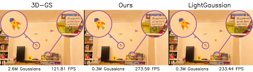
Figure 1: We prune the 3D-GS reconstruction of the Deep Blending playroom scene from $2.6$M Gaussians to $0.3$M Gaussians using our PUP 3D-GS pipeline and LightGaussian – a recent, high-performing post-hoc pruning pipeline for pretrained 3D-GS models. PUP 3D-GS retains more fine details while increasing the rendering speed from $121.81$ FPS to $273.29$ FPS, a $\boldsymbol{2.24\times}$ increase over the base 3D-GS model. In comparison, LightGaussian loses substantially more fine details and reaches a slower rendering speed of $233.44$ FPS. A detailed comparison of PUP 3D-GS and LightGaussian can be found in Section 5.3.2; additional per-scene metrics are recorded in Appendix A.1.

1 Introduction

Novel view synthesis aims to render views from new viewpoints given a set of 2D images. Neural Radiance Fields (NeRFs) [15] use volume rendering to represent the 3D scene using a multilayer perceptron that can be used to render novel views. Although NeRF and its variants achieve high-quality reconstructions, they have slow inference time and require several seconds to render a single image. 3D Gaussian Splatting (3D-GS) [9] has recently emerged as a faster alternative to NeRF, achieving real-time rendering on modern GPUs while producing comparable image quality. It represents scenes using a large set of 3D Gaussians with independent location, shape, and appearance parameters. Since they typically consist of millions of Gaussians, 3D-GS scenes often have high storage and memory requirements that limit their viability on devices with limited resources.

Several recent works propose techniques that reduce the storage requirements of 3D-GS models, including heuristics for pruning Gaussians that have an insignificant contribution to the rendered images [3, 4, 12, 18, 11]. In this work, we propose a more mathematically principled approach for deciding which Gaussians to prune from a 3D-GS scene. We introduce a computationally feasible sensitivity score that is derived from the Hessian of the reconstructed error on the training images in a converged scene. Following the methodology in LightGaussian [3], we prune the scene using our sensitivity score and then fine-tune the remaining Gaussians. Our experiments demonstrate that this process can remove up to $66\%$ of the Gaussians in the base 3D-GS scene while maintaining nearly identical image quality metrics.

Moreover, our approach enables a second consecutive round of pruning and fine-tuning. As shown in Figure 1, our multi-round pruning approach can remove over $88\%$ of the Gaussians in the base 3D-GS scene while surpassing previous heuristics-based methods like LightGaussian in both rendering speed and image quality. Our work is orthogonal to several other methods that modify the training framework of 3D-GS or apply quantization-based techniques to reduce its disk storage. We show that our PUP 3D-GS pipeline can be used in conjunction with these techniques to further improve performance and compress the model.

In summary, we propose the following contributions:

1. A post-hoc pruning pipeline, PUP 3D-GS, that can be applied to any pretrained 3D-GS model without changing its training pipeline.

2. A novel spatial sensitivity score that is more effective at pruning Gaussians than heuristics-based approaches.

3. A multi-round prune-refine approach that produces higher fidelity reconstructions than equivalent single-round prune-refining.

2 Related work

Neural Radiance Field (NeRF) based [15] approaches use neural networks to represent scenes and perform novel-view synthesis. They produce remarkable visual fidelity but suffer from slow training and inference. Recently, 3D Gaussian Splatting (3D-GS) [9] has emerged as an effective alternative for novel view synthesis, achieving faster inference speed and comparable visual fidelity to state-of-the-art NeRF-based approaches [1].

2.1 Uncertainty Estimation

Several works estimate uncertainty in NeRF-based approaches that arise from sources like transient objects, camera model differences, and lightning changes [8, 19, 20]. Other works focus on uncertainty caused by occlusion or sparsity of training views [14]. These approaches rely on an ensemble of models [24] or variational inference and KL Divergence [23, 22], requiring intricate changes to the training pipeline to model uncertainty.

BayesRays [5] uses Fisher information for post-hoc uncertainty quantification in NeRF-based approaches. Since NeRFs represent the scene as a continuous 3D function, they compute its Hessian over a hypothetical perturbation field to estimate uncertainty. In contrast, our approach focuses on 3D Gaussian Splats [9] instead of NeRF [14], and we directly compute the Fisher information using gradient information without relying on a hypothetical perturbation field.

FisherRF [7] also computes Fisher information for 3D Gaussian Splats; however, it only approximates the diagonal of the Fisher matrix and uses the color parameters (DC color and spherical harmonic coefficients) of the Gaussians for post-hoc uncertainty estimation. Our approach uses the spatial mean and scaling parameters to compute a more accurate block-wise approximation of the Fisher instead (see Section 4.1). Lastly, our work uses uncertainty estimates to prune Gaussians from the model, whereas FisherRF applies their method to perform active-view selection.

2.2 Pruning Gaussian Splat Models

While 3D-GS [9] demonstrates remarkable performance, it also entails substantial storage requirements. Several recent works use codebooks to quantize and reduce storage for various Gaussian parameters [11, 17, 18]. Others use the spatial relationships between neighboring Gaussians to reduce the number of parameters [13, 16, 2, 12]. Although these methods tout high compression rates, they modify the underlying primitives and training framework of 3D-GS. They also do not necessarily reduce the number of primitives and are, therefore, orthogonal to our work. We apply one such technique, Vectree Quantization [3], to further compress our pruned scenes in Section 5.3.3.

A recent pruning-based method, Compact-3DGS [11], proposes a learnable masking strategy to prune small, transparent Gaussians during training. EAGLES [4], which we apply our pipeline to in Appendix A.8, prunes Gaussians based on the least total transmittance per Gaussian. They also begin with low-resolution images, progressively increasing image resolution to reduce Gaussian densification during training, then quantize several attributes to reduce disk storage. LightGaussian [3] computes a global significance score for each Gaussian with heuristics, uses that score to prune the least significant Gaussians, and finally uses quantization to further reduce storage requirements.

3 Background

3.1 3D Gaussian Splatting

3D Gaussian Splatting (3D-GS) is a point-based novel view synthesis technique that uses 3D Gaussians to model the scene. The attributes of the Gaussians are optimized over input training views given by a set of camera poses $\mathcal{P}_{gt}=\{\phi_{i}\in{}^{3\times 4}\}_{i=1}^{K}$ and corresponding ground truth training images $\mathcal{I}_{gt}=\{\boldsymbol{I}_{i}\in{}^{H\times W}\}_{i=1}^{K}$. A sparse point cloud of the scene generated by Structure from Motion (SfM) over the training views is used to initialize the Gaussians. At fixed intervals during training, a Gaussian densification step is applied to increase the number of Gaussians in areas of the model where small-scale geometry is insufficiently reconstructed.

Each 3D Gaussian $\mathcal{G}_{i}$ is independently parameterized by position $x_{i}\in{}^{3}$, scaling $s_{i}\in{}^{3}$, rotation $r_{i}\in{}^{4}$, base color $c_{i}\in{}^{3}$, view-dependent spherical harmonics $h_{i}\in{}^{15\times 3}$, and opacity $\alpha_{i}\in\real$. From these, we define the set of all Gaussian parameters as:

$$\mathcal{G}=\{\mathcal{G}_{i}=\{x_{i},s_{i},r_{i},c_{i},h_{i},\alpha_{i}\}\}_{i=1}^{N},$$ (1)

where $N$ is the total number of Gaussians in the model.

During view synthesis, the scaling parameters $s_{i}$ and rotation parameters $r_{i}$ are converted into the scaling and rotation matrices $\boldsymbol{S}_{i}$ and $\boldsymbol{R}_{i}$. The Gaussian $\mathcal{G}_{i}$ is spatially characterized in the 3D scene by its center point, or mean position, $x_{i}$ and a decomposable covariance matrix $\boldsymbol{\Sigma}_{i}$:

$$\mathcal{G}_{i}(x_{i})=e^{-\frac{1}{2}x_{i}^{T}\boldsymbol{\Sigma}^{-1}_{i}x_{i}},\boldsymbol{\Sigma}_{i}=\boldsymbol{R}_{i}\boldsymbol{S}_{i}\boldsymbol{S}_{i}^{T}\boldsymbol{R}_{i}^{T}.$$ (2)

For a given camera pose $\phi$, a differential rasterizer renders 2D image $I_{\mathcal{G}}(\phi)$ by projecting all Gaussians observed from $\phi$ onto the image plane. The color of each pixel in $I_{\mathcal{G}}(\phi)$ is given by the blending of the $\mathcal{N}$ ordered Gaussians that overlap it:

$$C=\sum_{i\in\mathcal{N}}\tilde{c}_{i}\tilde{\alpha}_{i}\prod_{j=1}^{j-1}(1-\tilde{\alpha}_{j}),$$ (3)

where $\tilde{c}_{i}$ represents the view-dependent color calculated from the camera pose $\phi$ and the optimizable per-Gaussian color $c_{i}$ and spherical harmonics $h_{i}$, and $\tilde{\alpha_{i}}$ and $\tilde{\alpha_{j}}$ represent the projected opacities.

The 3D-GS model is trained by optimizing the loss function $L$ via stochastic gradient descent:

$$L(\mathcal{G}|\phi,I_{gt})=||I_{\mathcal{G}}(\phi)-I_{gt}||_{1}+L_{SSIM}(I_{\mathcal{G}}(\phi),I_{gt}),$$ (4)

where the first term is an L1 residual loss and the second term is an SSIM loss.

4 Method

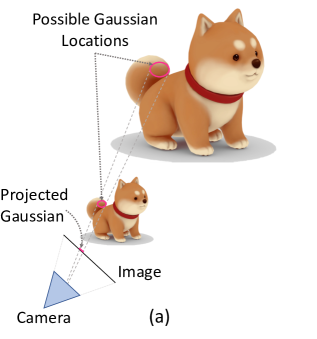
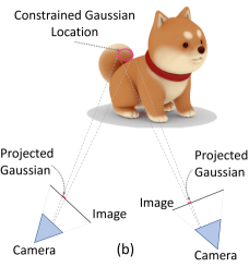
Figure 2: Spatial uncertainty arises from limited views because there are multiple possible 3D Gaussian locations that map to the same projected Gaussian in pixel space (a). This is reduced when multiple cameras observe previously unconstrained Gaussians (b).

3D scene reconstruction is an inherently underconstrained problem. Capturing a scene as a set of posed images $(\mathcal{P}_{gt},\mathcal{I}_{gt})$ involves projecting it onto the 2D image plane of each view. As illustrated by Figure 2, this introduces uncertainty in the locations and sizes of the Gaussians reconstructing the scene: a large Gaussian far from the camera can be equivalently modeled in pixel space by a small Gaussian close to the camera. In other words, Gaussians that are not perceived by a sufficient number of cameras may be able to reconstruct the input view image from a range of locations and scales.

We define uncertainty in 3D-GS as the amount that a Gaussian’s parameters, such as its location and scale, can be perturbed without affecting the reconstruction loss over the input views. Concretely, this is the sensitivity of the error over the input views to that particular Gaussian. Given a loss function $L:{}^{\mathcal{G}}\to\real$ that takes the set of Gaussians $\mathcal{G}$ as inputs and outputs an error value over the set of training views, this sensitivity can be captured by the Hessian $\nabla^{2}_{\mathcal{G}}L$.

In the following subsections, we demonstrate how to compute this sensitivity and use it to decide which Gaussians to prune from the model. Directly computing the full Hessian matrix is intractable due to memory constraints. We demonstrate how to obtain a close estimate of the Hessian via a Fisher approximation in Section 4.1. We also find that only a block-wise approximation of the Hessian parameters is needed to quantify Gaussian sensitivity in Section 4.2, and that computing this over image patches instead of pixels reduces compute and is sufficient for pruning in Section 4.3. Finally, we find that multiple rounds of pruning and fine-tuning improves our performance over one-shot pruning and fine-tuning, giving our full PUP 3D-GS pipeline in Section 4.4.

4.1 Fisher Approximation

To obtain a per-Gaussian sensitivity, we begin by taking the $L_{2}$ error over the input reconstruction images $I_{\mathcal{G}}$:

$$L_{2}=\frac{1}{2}\sum_{\phi\in\mathcal{P}_{gt}}||I_{\mathcal{G}}(\phi)-I_{gt}||_{2}^{2}.$$ (5)

Differentiating this twice gives us the Hessian:

$$\nabla_{\mathcal{G}}^{2}L_{2}=\sum_{\phi\in\mathcal{P}_{gt}}\nabla_{\mathcal{G}}I_{\mathcal{G}}(\phi)\nabla_{\mathcal{G}}I_{\mathcal{G}}(\phi)^{T}+(I_{\mathcal{G}}(\phi)-I_{gt})\nabla_{\mathcal{G}}^{2}I_{\mathcal{G}}(\phi).$$ (6)

On a converged 3D-GS model, the $||I_{\mathcal{G}}-I_{gt}||_{1}$ residual term of Equation 4 approaches zero, causing the second order term $(I_{\mathcal{G}}(\phi)-I_{gt})\nabla_{\mathcal{G}}^{2}I_{\mathcal{G}}$ in Equation 6 to vanish. This leaves us with:

$$\nabla_{\mathcal{G}}^{2}L_{2}=\nabla_{\mathcal{G}}I_{\mathcal{G}}\nabla_{\mathcal{G}}I_{\mathcal{G}}^{T},$$ (7)

which is known as a Fisher approximation of the Hessian [5, 7].

Note that $\nabla_{\mathcal{G}}I_{\mathcal{G}}$ is the gradient over only the reconstructed images. This means that our approximation only depends on the input poses $\mathcal{P}_{gt}$ and not the input images $\mathcal{I}_{gt}$. However, our Fisher approximation of $\nabla_{\mathcal{G}}^{2}L_{2}$ is still computationally expensive as it requires a sum over all per-pixel Fisher approximations of the scene. We describe how we make this more efficient in Section 4.3.

4.2 Sensitivity Pruning Score

The full Hessian over the model parameters $\nabla_{\mathcal{G}}^{2}L\in{}^{\mathcal{G}\times\mathcal{G}}$ is quadratically large. However, we find that using only a fraction of these parameters is sufficient for an effective sensitivity pruning score.

To obtain sensitivity scores for each Gaussian $\mathcal{G}_{i}$, we restrict ourselves to the block diagonal of the Hessian that only captures inter-Gaussian parameter relationships. This allows us to use each block as a per-Gaussian Hessian from which we can obtain an independent sensitivity score:

$$\boldsymbol{H}_{i}=\nabla_{\mathcal{G}_{i}}I_{\mathcal{G}_{i}}\nabla_{\mathcal{G}_{i}}I_{\mathcal{G}_{i}}^{T}.$$ (8)

Intuitively, each of these block Hessians measures the impact on the reconstruction error when we perturb the parameters of only the Gaussian it represents. To turn each Hessian $\boldsymbol{H}_{i}$ into a single value sensitivity score ${\tilde{U}}_{i}\in\real$, we take the log determinant of $\boldsymbol{H}_{i}$:

$${\tilde{U}}_{i}=\log|\boldsymbol{H}_{i}|=\log|\nabla_{\mathcal{G}_{i}}I_{\mathcal{G}_{i}}\nabla_{\mathcal{G}_{i}}I_{\mathcal{G}_{i}}^{T}|.$$ (9)

This captures the relative impact over all of the parameters of Gaussian $\mathcal{G}_{i}$ on the reconstruction error. Specifically, it is a relative volume measure of the basin around the Gaussian parameters $\mathcal{G}_{i}$ in the second-order approximation of the function describing their impact on the reconstruction error.

We find that we can restrict the per Gaussian parameters even further and consider only the spatial mean $x_{i}$ and scaling $s_{i}$ parameters for an effective sensitivity score. Our final sensitivity pruning score $U_{i}\in\real$ is:

$$U_{i}=\log|\nabla_{x_{i},s_{i}}I_{\mathcal{G}_{i}}\nabla_{x_{i},s_{i}}I_{\mathcal{G}_{i}}^{T}|.$$ (10)

We speculate that only the spatial mean and scaling parameters are needed because they capture the projective geometric invariances that exist between the 3D scene and the input views as shown in Figure 2. We ablate the choice of using spatial parameters in Section 6.2.

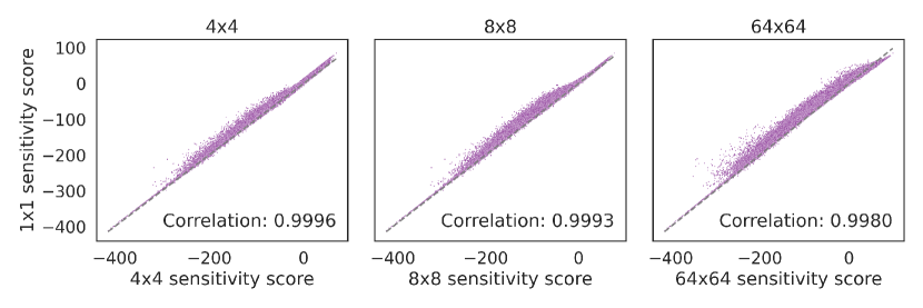
Figure 3: Spearman correlations between the $1\times 1$ pixel-wise sensitivity score and the $4\times 4$, $8\times 8$, and $64\times 64$ patch-wise sensitivity scores across all Gaussians in the Tanks & Temples truck scene. Notice that the correlation remains very high even with a large patch size of $64\times 64$.

Table 1: Mean PSNR, SSIM, LPIPS, FPS, and point cloud size for the Mip-NeRF 360 dataset at each stage of our PUP 3D-GS pipeline. The operation in each row is applied cumulatively to all of the following rows. Per-scene metrics across all datasets are recorded in Appendix A.1.

Methods	PSNR$\uparrow$	SSIM$\uparrow$	LPIPS$\downarrow$	FPS$\uparrow$	Size (MB)$\downarrow$
3D-GS	27.47	0.8123	0.2216	95.59	746.46
+ Prune $66\%$	25.60	0.7836	0.2497	178.23	253.8
+ Refine	27.50	0.8122	0.2281	153.27	253.8
+ Prune $66\%$	20.35	0.6718	0.3441	310.73	86.29
+ Refine	26.83	0.792	0.2688	244.07	86.29

4.3 Patch-wise Uncertainty

As mentioned in Section 4.1, the computation of the Hessian over the entire scene requires a sum over all per-pixel Fisher approximations of the reconstructed input views. However, we empirically observe that our sensitivity scores computed over image patches maintain a high correlation with our sensitivity scores computed over individual pixels. Specifically, we compute the Fisher approximation on image patches by applying an average pool over each $n\times n$ block of pixels in the rendered images, then compute the Fisher approximation on each pixel of the downsampled image. To obtain the scene-level Hessian we sum all patch-wise Fisher approximations over all images. In our experiments, we compute Fisher approximations over $8\times 8$ image patches, but Figure 3 illustrates that the correlation with per-pixel scores is maintained even with larger patches of size $64\times 64$. We further ablate our choice of patch size in Appendix A.3.

4.4 Multi-Round Pipeline

Similar to LightGaussian [3], we prune the model and then fine-tune it without further Gaussian densification. For brevity, we will refer to this process as prune-refine. We find that, in many circumstances, the model is able to recover the small $||I_{\mathcal{G}}-I_{gt}||_{1}$ residual after fine-tuning, allowing us to repeat prune-refine over multiple rounds. We empirically notice that multiple rounds of prune-refine outperforms an equivalent single round of prune-refine. Details of this evaluation are in Section 6.1.

5 Experiments

5.1 Datasets

We evaluate our approach on the same challenging, real world scenes as 3D-GS [9]. All nine scenes from the MiP-NeRF 360 dataset [1], which consists of five outdoor and four indoor scenes that each contain a complex central object or viewing area and a detailed background, are used. Two outdoor scenes, truck and train, are taken from the Tanks & Temples dataset [10], and two indoor scenes, drjohnson and playroom, are taken from the Deep Blending dataset [6]. For consistency, we use the COLMAP [21] camera pose estimates that are provided by the creators of the datasets.

5.2 Implementation Details

Our method, PUP 3D-GS, can be applied to any 3D-GS model. We implement the Hessian computation on the original 3D-GS codebase [9], then adapt the pruning and refining framework from LightGaussian [3] to accommodate our uncertainty estimate and multi-round pruning method. For a fair comparison, we run LightGaussian and our pipeline on the same pretrained 3D-GS scenes. Rendering speeds are collected using a Nvidia RTXA5000 GPU in frames per second (FPS).

5.3 Results

5.3.1 Analysis of PUP 3D-GS Pipeline

The efficacy of our PUP 3D-GS pipeline is demonstrated by Table 1, where we record the mean of each metric over the Mip-NeRF 360 dataset. Pruning $66\%$ of Gaussians from the original 3D-GS model nearly doubles its FPS with only a small degradation of PSNR, SSIM, and LPIPS. Fine-tuning the pruned model for 5,000 iterations recovers the image quality metrics while only slightly decreasing rendering speed. Pruning $66\%$ of the remaining Gaussians, such that a total of $88.44\%$ of Gaussians are pruned from the base 3D-GS scene, causes a larger drop in the image quality metrics. However, we recover most of this degradation by fine-tuning this significantly smaller model for another 5,000 iterations. Rendering speed is nearly tripled.

5.3.2 Comparison with LightGaussian

Table 2 compares our $88.44\%$ pruning results against LightGaussian’s using the per-dataset mean of each metric. For our method, we run the full two step prune-refine pipeline described in Section 5.3.1, where we perform two rounds of $66\%$ pruning using our spatial uncertainty estimate with 5,000 fine-tuning iterations each. In LightGaussian, we run their one-round pipeline to prune $88.44\%$ of Gaussians using their global significance score and then fine-tune for 10,000 iterations. In LightGaussian ($2\times$), we use their global significance score in our two step prune-refine pipeline.

We show that our spatial uncertainty estimate outperforms both configurations of LightGaussian across nearly every metric. The lone exception is PSNR on the Tanks & Temples dataset, where we are slightly outperformed by LightGaussian by less than 0.06 points.

Table 2: Comparison of our PUP 3D-GS pipeline against LightGaussian [3]. For a fairness, we record the results of the original LightGaussian pipeline which uses a single prune-refine step and the results of applying our multi-round pruning to the LightGaussian pipeline, LightGaussian (2$\times$), where we run their prune-refine step twice. The original LightGaussian pipeline prunes to $88.44\%$ once, while our pipeline and LightGaussian (2$\times$) prune $66\%$ twice for a total of $88.44\%$: the final sizes are identical. PUP 3D-GS increases the rendering speed of 3D-GS by $2.65\times$ on average.

Datasets	Methods	PSNR$\uparrow$	SSIM$\uparrow$	LPIPS$\downarrow$	FPS$\uparrow$	Size (MB)$\downarrow$
MipNerf-360	3D-GS	27.47	0.812	0.221	95.59	746.46
	LightGaussian	26.25	0.763	0.298	177.4	86.29
	LightGaussian (2$\times$)	26.18	0.761	0.304	191.36	86.29
	Ours	26.83	0.792	0.268	244.07	86.29
Tanks & Temples	3D-GS	23.77	0.845	0.1777	147.97	433.24
	LightGaussian	23.09	0.797	0.2603	370.42	50.08
	LightGaussian (2$\times$)	23.03	0.793	0.2663	320.12	50.08
	Ours	23.03	0.807	0.2453	417.98	50.08
Deep Blending	3D-GS	28.98	0.8816	0.2856	105.61	699.19
	LightGaussian	28.35	0.8676	0.3333	240.17	80.83
	LightGaussian (2$\times$)	28.11	0.8647	0.3373	210.12	80.83
	Ours	28.61	0.8812	0.3053	296.08	80.83

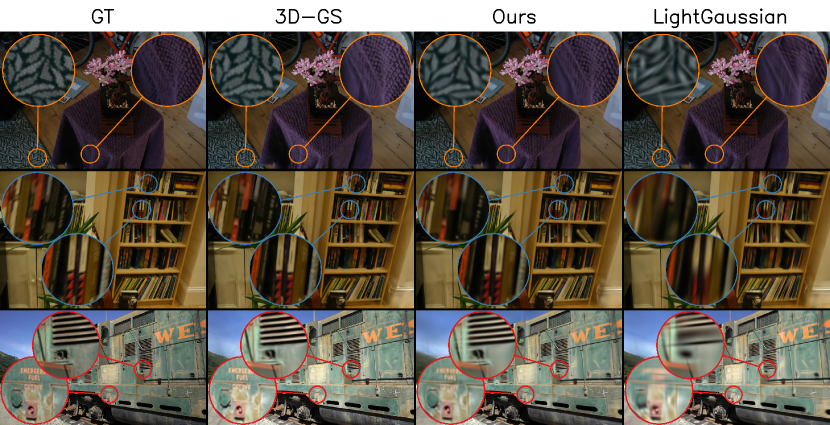
Figure 4: Visual comparison after two rounds of prune-refine using our method and LightGaussian’s method. Top: bonsai from the Mip-Nerf 360 dataset. Middle: room from the Mip-Nerf 360 dataset. Bottom: train from the Tanks & Temples dataset. Additional visual results are in Appendix A.2

In Figure 4, we report qualitative results on one scene taken from each dataset. The magnified regions demonstrate that our method retains many fine foreground details that are not preserved by LightGaussian. Error residual images with respect to the ground truth and original 3D-GS scenes are available in Appendix A.6 and Appendix A.7; visualizations of other scenes are provided in Appendix A.2.

We speculate that the visibility score in LightGaussian’s importance sampling heuristic is biased towards retaining larger Gaussian because they have a higher probability of being visible in more pixels across the training views. In Figure 5, we plot the distribution of the log determinant of the Gaussian covariances over the scenes visualized in Figure 4. The distribution clearly skews more heavily towards larger Gaussians in the scenes pruned with LightGaussian than our pipeline.

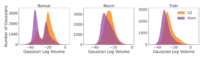
Figure 5: Histograms showing the distribution of Gaussians over the log of their volumes for the bonsai, room, and train scenes after two rounds of prune-refine with our PUP 3D-GS pipeline and LightGaussian’s pipeline (LG). LightGaussian consistently retains larger Gaussians than ours.

5.3.3 Vectree Quantization

We apply the Vector Quantization implementation found in the LightGaussian framework to further compress our pruned models. Our final average model sizes are $16.76$MB for Mip-NeRF 360, $9.87$MB for Tanks & Temples, and $15.64$MB on Deep Blending. In other words, the unpruned 3D-GS scenes are reduced in size by $44.5\times$, $43.9\times$, and $44.7\times$, respectively.

Table 3: Vectree Quantization comparison with LightGaussian after pruning to $88.44\%$. Similar to Table 2, we report quantization on the original one-round LightGaussian method as well LightGaussian with two rounds of prune-refine. PUP 3D-GS outperforms LightGaussian across all metrics.

Datasets	Methods	PSNR$\uparrow$	SSIM$\uparrow$	LPIPS$\downarrow$	FPS$\uparrow$	Size (MB)$\downarrow$
Mip-NeRF 360	3D-GS	27.47	0.8123	0.2216	95.59	746.46
	LightGaussian	24.61	0.7272	0.3313	217.64	16.8
	LightGaussian (2$\times$)	24.58	0.7252	0.3318	199.1	16.81
	Ours	25.05	0.7599	0.2963	257.57	16.76
Tanks & Temples	3D-GS	23.77	0.8458	0.1777	147.97	433.24
	LightGaussian	21.80	0.7666	0.2897	412.94	9.91
	LightGaussian (2$\times$)	21.80	0.7668	0.2896	367.87	9.92
	Ours	21.81	0.7837	0.2673	428.59	9.87
Deep Blending	3D-GS	28.98	0.8816	0.2859	105.61	699.19
	LightGaussian	27.66	0.8564	0.3467	238.94	15.65
	LightGaussian (2$\times$)	27.37	0.8526	0.3474	254.64	15.65
	Ours	27.79	0.8700	0.3146	351.72	15.64

6 Ablations

6.1 Multi-Round vs. One-Round Pipeline

A core component of our pipeline is running prune-refine over multiple rounds. In Table 4, we compare the mean image quality and FPS over the Mip-NeRF 360 scenes when we prune using our two step prune-refine method against when we prune 88.44% of Gaussians in one round. Multi-round pruning produces better measurements across all metrics.

Table 4: One step of pruning $88.44\%$ of Gaussians from 3D-GS and then fine-tuning for 10,000 iterations, versus two steps of pruning $66\%$ of Gaussians and finetuning for 5,000 iterations each. In both cases, $88.44\%$ Gaussians are pruned and the model is fine-tuned for 10,000 total steps. Our multi-round approach outperforms the one-round approach across all metrics.

Methods	Mip-NeRF 360
	PSNR$\uparrow$	SSIM$\uparrow$	LPIPS$\downarrow$	FPS$\uparrow$	Size (MB)$\downarrow$
3D-GS	27.47	0.8123	0.2216	95.59	746.46
Prune $88.44\%+10$K Finetune	26.51	0.7864	0.2731	221.34	86.29
(Prune $66\%+5$K Finetune) $\times 2$	26.83	0.7920	0.2688	244.07	86.29

6.2 Spatial vs. Color Parameters

Another component of our method is restricting our sensitivity pruning score to only the mean and scale parameters for each Gaussian. Table 5 shows that image quality decreases if we use the RGB color parameters of the Gaussians to compute our sensitivity score instead. We speculate that the lower performance of the RGB sensitivity score is due to its similarity with LightGaussian’s visibility score – the change in the L2 error over the training images with respect to perturbations in the RGB value of a Gaussian correlates with its visibility across the training views.

Table 5: Results from our two step prune-refine pipeline when computing sensitivity with spatial and RGB color parameters. The spatial score produces higher fidelity renderings than the color score.

Methods	Mip-NeRF 360 Bicycle Scene
	PSNR$\uparrow$	SSIM$\uparrow$	LPIPS$\downarrow$	FPS$\uparrow$	Size (MB)$\downarrow$
3D-GS	25.09	0.7467	0.2442	50.23	1345.58
RGB Sensitivity	24.73	0.7155	0.2963	160.81	155.55
Spatial Sensitivity	25.00	0.7270	0.2870	139.67	155.55

7 Limitations

A limitation of our approach is that it assumes that the scene is converged because the Fisher approximation requires a small L1 residual to be accurate. We find that a small residual is preserved even after removing $66\%$ of the Gaussians with prune-refine, allowing us to perform a second round, as shown in Section 4.4. Our Fisher approximation also involves computational overhead that is reduced by performing it in the patch-wise manner described in Section 4.3. We are optimistic that more sophisticated techniques like optimized CUDA kernels and data parallelization can further improve the efficiency of our approximation.

8 Conclusion

In this work, we propose PUP 3D-GS: a new post-hoc pipeline for pruning pretrained 3D-GS models without changing their training pipelines. It uses a novel, mathematically principled approach for choosing which Gaussians to prune by assessing their sensitivity to the reconstruction error over the training views. This sensitivity pruning score is derived from a computationally tractable Fisher approximation of the Hessian over that reconstruction error. We use our sensitivity score to prune the reconstructed scene, then fine-tune the remaining Gaussians in the model over multiple rounds. We observe that PUP 3D-GS improves the rendering speed of 3D-GS by $2.65\times$ on average, while retaining more salient foreground information than existing techniques and achieving higher image quality metrics on the MiP-NeRF 360, Tanks & Temples, and Deep Blending dataset scenes.

9 Acknowledgements

This research is based upon work supported by the Office of the Director of National Intelligence (ODNI), Intelligence Advanced Research Projects Activity (IARPA), via IARPA R&D Contract No. 140D0423C0076. The views and conclusions contained herein are those of the authors and should not be interpreted as necessarily representing the official policies or endorsements, either expressed or implied, of the ODNI, IARPA, or the U.S. Government. The U.S. Government is authorized to reproduce and distribute reprints for Governmental purposes notwithstanding any copyright annotation thereon. Additional support was provided by ONR MURI program and the AFOSR MURI program. Commercial support was provided by Capital One Bank, the Amazon Research Award program, and Open Philanthropy. Zwicker was additionally supported by the National Science Foundation (IIS-2126407). Goldstein was additionally supported by the National Science Foundation (IIS-2212182) and by the NSF TRAILS Institute (2229885).

Appendix A Appendix

A.1 Scene Evaluations

PSNR, SSIM, LPIPS, and FPS for each scene from the Mip-NeRF 360, Tanks&Temples, and Deep Blending datasets that was used in 3D-GS [9]. Note that the sizes of the pruned scenes in this section are identical because exactly $88.44\%$ of Gaussians were removed from each of them using our two step prune-refine method.

Table 6: PSNR on each scene after two steps of prune-refine.

Methods	Mip-NeRF 360									Tanks&Temples		Deep Blending
	bicycle	bonsai	counter	flowers	garden	kitchen	room	stump	treehill	train	truck	drjohnson	playroom
Baseline (3D-GS)	25.09	32.25	29.11	21.34	27.28	31.57	31.51	26.55	22.56	22.10	25.43	28.15	29.81
LightGaussian	24.35	29.41	27.40	20.59	25.90	29.26	30.42	25.77	22.51	21.28	24.77	27.29	28.92
Ours	24.99	30.62	28.11	21.09	26.66	29.99	31.13	26.39	22.52	21.32	24.73	27.63	29.58

Table 7: SSIM on each scene after two steps of prune-refine.

Methods	Mip-NeRF 360									Tanks&Temples		Deep Blending
	bicycle	bonsai	counter	flowers	garden	kitchen	room	stump	treehill	train	truck	drjohnson	playroom
Baseline (3D-GS)	0.7467	0.9457	0.9140	0.5875	0.8558	0.9317	0.9255	0.7687	0.6352	0.8134	0.8782	0.8778	0.8854
LightGaussian	0.6801	0.8921	0.8562	0.5343	0.7833	0.8830	0.8989	0.7256	0.5956	0.7349	0.8512	0.8546	0.8747
Ours	0.7270	0.9261	0.8917	0.5548	0.8189	0.9128	0.9152	0.7570	0.6248	0.7600	0.8541	0.8762	0.8861

Table 8: LPIPS on each scene after two steps of prune-refine.

Methods	Mip-NeRF 360									Tanks&Temples		Deep Blending
	bicycle	bonsai	counter	flowers	garden	kitchen	room	stump	treehill	train	truck	drjohnson	playroom
Baseline (3D-GS)	0.2442	0.1811	0.1838	0.3602	0.1225	0.1165	0.1973	0.2429	0.3460	0.2077	0.1476	0.2895	0.2823
LightGaussian	0.3318	0.2600	0.2828	0.4259	0.2291	0.2069	0.2616	0.3155	0.4261	0.3287	0.2039	0.3482	0.3264
Ours	0.2870	0.2304	0.2323	0.4196	0.1859	0.1569	0.2271	0.2784	0.4016	0.2981	0.1925	0.3316	0.2990

Table 9: FPS on each scene after two steps of prune-refine.

Methods	Mip-NeRF 360									Tanks&Temples		Deep Blending
	bicycle	bonsai	counter	flowers	garden	kitchen	room	stump	treehill	train	truck	drjohnson	playroom
Baseline (3D-GS)	50.23	130.25	123.76	106.47	60.86	98.47	115.75	87.80	86.76	167.53	128.40	90.42	120.81
LightGaussian	114.51	229.01	198.98	241.87	163.21	188.01	181.04	218.44	187.17	404.51	235.72	186.80	233.44
Ours	139.67	297.42	268.49	272.12	201.04	296.71	255.86	222.75	242.61	521.98	313.98	318.57	273.59

A.2 Additional Scene Visualizations

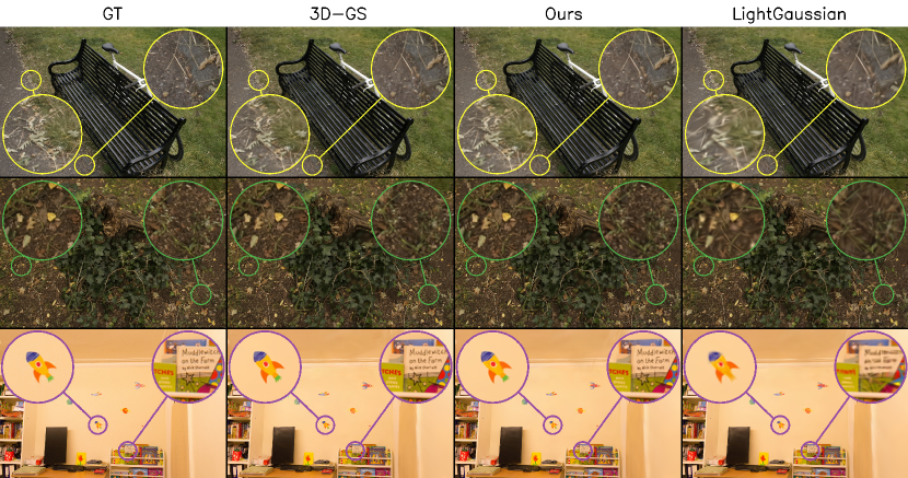
Figure 6: Visual comparison after two rounds of prune-refine using our method and LightGaussian’s method. Top: bicycle from the Mip-Nerf 360 dataset. Middle: stump from the Mip-Nerf 360 dataset. Bottom: playroom from the Deep Blending dataset. A larger example image of playroom can be found in Figure 1

A.3 Ablation on Patch Size

Table 10: Results of pruning the Tanks&Temples truck scene using our sensitivity score computed with $8\times 8$ and $64\times 64$ patches. Notice that, although the $8\times 8$ patches that we use in our experiments measures slightly better across all metrics, the $64\times 64$ size patches produce similar results.

Methods	Tanks&Temples Truck Scene
	PSNR$\uparrow$	SSIM$\uparrow$	LPIPS$\downarrow$	FPS$\uparrow$	Size (MB)$\downarrow$
3D-GS	25.43	0.8782	0.1476	128.40	610.19
$8\times 8$	24.73	0.8541	0.1925	313.98	70.54
$64\times 4$	24.63	0.8501	0.1973	312.81	70.54

A.4 Ablation on Number of Prune-Refine Steps

Table 11: Results from pruning a total of 88.44% of the Gaussians using one, two, and three steps of prune-refine over 10,000 total iterations of refinement. Our two-step method achieves the highest image fidelity.

Methods	Mip-NeRF 360 Bicycle Scene
	PSNR$\uparrow$	SSIM$\uparrow$	LPIPS$\downarrow$	FPS$\uparrow$	Size (MB)$\downarrow$
Baseline (3D-GS)	25.09	0.7467	0.2442	50.23	1345.58
+ $88.44\%+10000$	24.83	0.7177	0.2916	95.77	155.55
+ $(66\%+5000)\times 2$	24.99	0.7270	0.2870	139.67	155.55
+ $(51.29\%+3333)\times 3$	24.91	0.7270	0.2875	164.63	155.55

A.5 Ablation on Pruning Percentage

Table 12: Results from two steps of prune-refine with 50%, 66%, and 75% pruning and 5000 refinement iterations per-step. Our 66% pruning method balances the higher fidelity of 50% pruning with the improved FPS and file size of 75% pruning.

Methods	Mip-NeRF 360 Bicycle Scene
	PSNR$\uparrow$	SSIM$\uparrow$	LPIPS$\downarrow$	FPS$\uparrow$	Size (MB)$\downarrow$
Baseline (3D-GS)	25.09	0.7467	0.2442	50.23	1345.58
+ $(50\%+5000)\times 2$	25.19	0.7459	0.2537	93.54	336.40
+ $(66\%+5000)\times 2$	24.99	0.7270	0.2870	139.67	155.55
+ $(75\%+5000)\times 2$	24.67	0.6995	0.3269	174.86	84.10

A.6 Scene Ground Truth Residuals

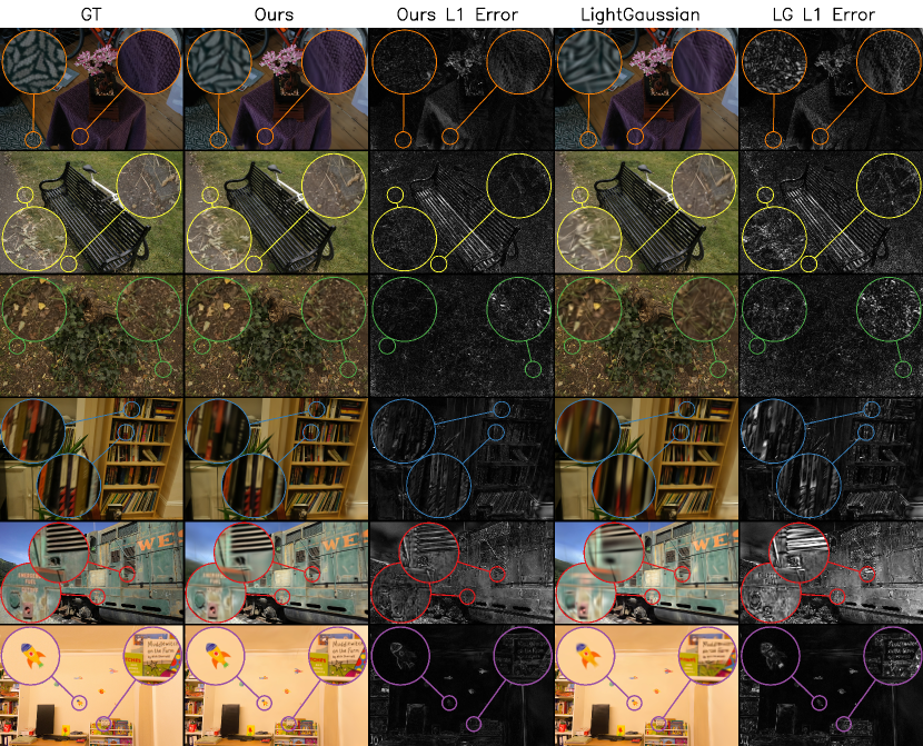
Figure 7: Visual comparison of our method with LightGaussian after removing $88.44\%$ of Gaussians with added ground truth L1 error visualizations. Columns "GT", "Ours", and "LightGaussian" are the same as in Figure 4. Columns "Ours L1 Error" and "LG L1 Error" are the L1 Error images of our method and LightGaussian against the ground truth images.

A.7 Scene 3D-GS Residuals

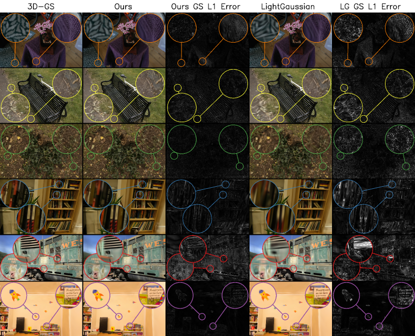
Figure 8: Visual comparison after two rounds of prune-refine using our method and LightGaussian’s. with added ground truth L1 error visualizations. Columns "3D-GS", "Ours", and "LightGaussian" are the same as in Figure 4. Columns "Ours GS L1 Error" and "LG GS L1 Error" are the L1 error images of our method and LightGaussian against the original 3D-GS reconstruction of the scene.

A.8 Prune-Refining EAGLES

Table 13: Results from training EAGLES [4] on the bicycle scene and then running two steps of prune-refine. Notice that the base EAGLES model produces similar metrics to vanilla 3D-GS despite being $2.51\times$ smaller than it. By applying PUP 3D-GS to the EAGLES model, we further reduce its size to $7.39\times$ smaller than the vanilla 3D-GS model while achieving better image quality than LightGaussian, which attains slightly higher rendering speed.

Methods	Mip-NeRF 360 Bicycle Scene
	PSNR$\uparrow$	SSIM$\uparrow$	LPIPS$\downarrow$	FPS$\uparrow$	Size (MB)$\downarrow$
3D-GS	25.09	0.7467	0.2442	50.23	1345.58
Baseline (EAGLES)	25.07	0.7508	0.2433	58.70	535.21
EAGLES + LightGaussian	24.52	0.7018	0.3094	91.26	181.97
EAGLES + Ours	24.78	0.7212	0.2870	83.13	181.97

References

- [1] Jonathan T Barron, Ben Mildenhall, Dor Verbin, Pratul P Srinivasan, and Peter Hedman. Mip-nerf 360: Unbounded anti-aliased neural radiance fields. In Proceedings of the IEEE/CVF Conference on Computer Vision and Pattern Recognition, pages 5470–5479, 2022.
- [2] Yihang Chen, Qianyi Wu, Jianfei Cai, Mehrtash Harandi, and Weiyao Lin. Hac: Hash-grid assisted context for 3d gaussian splatting compression. arXiv preprint arXiv:2403.14530, 2024.
- [3] Zhiwen Fan, Kevin Wang, Kairun Wen, Zehao Zhu, Dejia Xu, and Zhangyang Wang. Lightgaussian: Unbounded 3d gaussian compression with 15x reduction and 200+ fps. arXiv preprint arXiv:2311.17245, 2023.
- [4] Sharath Girish, Kamal Gupta, and Abhinav Shrivastava. Eagles: Efficient accelerated 3d gaussians with lightweight encodings. arXiv preprint arXiv:2312.04564, 2023.
- [5] Lily Goli, Cody Reading, Silvia Selllán, Alec Jacobson, and Andrea Tagliasacchi. Bayes’ rays: Uncertainty quantification for neural radiance fields. Proceedings of the IEEE/CVF Conference on Computer Vision and Pattern Recognition, 2024.
- [6] Peter Hedman, Julien Philip, True Price, Jan-Michael Frahm, George Drettakis, and Gabriel Brostow. Deep blending for free-viewpoint image-based rendering. ACM Transactions on Graphics, 37(6):1–15, 2018.
- [7] Wen Jiang, Boshu Lei, and Kostas Daniilidis. Fisherrf: Active view selection and uncertainty quantification for radiance fields using fisher information. arXiv preprint arXiv:2311.17874, 2023.
- [8] Liren Jin, Xieyuanli Chen, Julius Rückin, and Marija Popović. Neu-nbv: Next best view planning using uncertainty estimation in image-based neural rendering. In IEEE/RSJ International Conference on Intelligent Robots and Systems, pages 11305–11312. IEEE, 2023.
- [9] Bernhard Kerbl, Georgios Kopanas, Thomas Leimkühler, and George Drettakis. 3d gaussian splatting for real-time radiance field rendering. ACM Transactions on Graphics, 42(4):1–14, 2023.
- [10] Arno Knapitsch, Jaesik Park, Qian-Yi Zhou, and Vladlen Koltun. Tanks and temples: Benchmarking large-scale scene reconstruction. ACM Transactions on Graphics, 36(4):1–13, 2017.
- [11] Joo Chan Lee, Daniel Rho, Xiangyu Sun, Jong Hwan Ko, and Eunbyung Park. Compact 3d gaussian representation for radiance field. arXiv preprint arXiv:2311.13681, 2023.
- [12] Xiangrui Liu, Xinju Wu, Pingping Zhang, Shiqi Wang, Zhu Li, and Sam Kwong. Compgs: Efficient 3d scene representation via compressed gaussian splatting. arXiv preprint arXiv:2404.09458, 2024.
- [13] Tao Lu, Mulin Yu, Linning Xu, Yuanbo Xiangli, Limin Wang, Dahua Lin, and Bo Dai. Scaffold-gs: Structured 3d gaussians for view-adaptive rendering. arXiv preprint arXiv:2312.00109, 2023.
- [14] Ricardo Martin-Brualla, Noha Radwan, Mehdi SM Sajjadi, Jonathan T Barron, Alexey Dosovitskiy, and Daniel Duckworth. Nerf in the wild: Neural radiance fields for unconstrained photo collections. In Proceedings of the IEEE/CVF Conference on Computer Vision and Pattern Recognition, pages 7210–7219, 2021.
- [15] Ben Mildenhall, Pratul P Srinivasan, Matthew Tancik, Jonathan T Barron, Ravi Ramamoorthi, and Ren Ng. Nerf: Representing scenes as neural radiance fields for view synthesis. Communications of the ACM, 65(1):99–106, 2021.
- [16] Wieland Morgenstern, Florian Barthel, Anna Hilsmann, and Peter Eisert. Compact 3d scene representation via self-organizing gaussian grids. arXiv preprint arXiv:2312.13299, 2023.
- [17] KL Navaneet, Kossar Pourahmadi Meibodi, Soroush Abbasi Koohpayegani, and Hamed Pirsiavash. Compact3d: Compressing gaussian splat radiance field models with vector quantization. arXiv preprint arXiv:2311.18159, 2023.
- [18] Simon Niedermayr, Josef Stumpfegger, and Rüdiger Westermann. Compressed 3d gaussian splatting for accelerated novel view synthesis. arXiv preprint arXiv:2401.02436, 2023.
- [19] Xuran Pan, Zihang Lai, Shiji Song, and Gao Huang. Activenerf: Learning where to see with uncertainty estimation. In European Conference on Computer Vision, pages 230–246. Springer, 2022.
- [20] Sara Sabour, Suhani Vora, Daniel Duckworth, Ivan Krasin, David J Fleet, and Andrea Tagliasacchi. Robustnerf: Ignoring distractors with robust losses. In Proceedings of the IEEE/CVF Conference on Computer Vision and Pattern Recognition, pages 20626–20636, 2023.
- [21] Johannes L Schonberger and Jan-Michael Frahm. Structure-from-motion revisited. In Proceedings of the IEEE/CVF Conference on Computer Vision and Pattern Recognition, pages 4104–4113, 2016.
- [22] Jianxiong Shen, Antonio Agudo, Francesc Moreno-Noguer, and Adria Ruiz. Conditional-flow nerf: Accurate 3d modelling with reliable uncertainty quantification. In European Conference on Computer Vision, pages 540–557. Springer, 2022.
- [23] Jianxiong Shen, Adria Ruiz, Antonio Agudo, and Francesc Moreno-Noguer. Stochastic neural radiance fields: Quantifying uncertainty in implicit 3d representations. In 2021 International Conference on 3D Vision, pages 972–981. IEEE, 2021.
- [24] Niko Sünderhauf, Jad Abou-Chakra, and Dimity Miller. Density-aware nerf ensembles: Quantifying predictive uncertainty in neural radiance fields. In 2023 IEEE International Conference on Robotics and Automation, pages 9370–9376. IEEE, 2023.