A Fundamental Trade-off in Aligned Language Models and its Relation to Sampling Adaptors

Abstract

The relationship between the quality of a string and its probability ${p}({\boldsymbol{y}})$ under a language model has been influential in the development of techniques to build good text generation systems. For example, several decoding algorithms have been motivated to manipulate ${p}({\boldsymbol{y}})$ to produce higher-quality text. In this work, we examine the probability–quality relationship in language models explicitly aligned to human preferences, e.g., through Reinforcement Learning through Human Feedback (RLHF). We find that, given a general language model and its aligned version, for corpora sampled from an aligned language model, there exists a trade-off between the average reward and average log-likelihood of the strings under the general language model. We provide a formal treatment of this issue and demonstrate how a choice of sampling adaptor allows for a selection of how much likelihood we exchange for the reward.

https://github.com/tanyjnaaman/probability-quality-paradox

A Fundamental Trade-off in Aligned Language Models and its Relation to Sampling Adaptors

Naaman Tan${}^{\leavevmode\raisebox{-0.70004pt}{\includegraphics[height=6.29996pt]{emoji_src/palm_tree.png}}}$  Josef Valvoda${}^{\leavevmode\raisebox{-0.70004pt}{\includegraphics[height=6.29996pt]{emoji_src/umbrella.png}}}$ Tianyu Liu${}^{\leavevmode\raisebox{-0.70004pt}{\includegraphics[height=6.29996pt]{emoji_src/chocolate_bar.png}}}$ Anej Svete${}^{\leavevmode\raisebox{-0.70004pt}{\includegraphics[height=6.29996pt]{emoji_src/chocolate_bar.png}}}$ Yanxia Qin${}^{\leavevmode\raisebox{-0.70004pt}{\includegraphics[height=6.29996pt]{emoji_src/palm_tree.png}}}$ Kan Min-Yen${}^{\leavevmode\raisebox{-0.70004pt}{\includegraphics[height=6.29996pt]{emoji_src/palm_tree.png}}}$ Ryan Cotterell${}^{\leavevmode\raisebox{-0.70004pt}{\includegraphics[height=6.29996pt]{emoji_src/chocolate_bar.png}}}$ ${}^{\leavevmode\raisebox{-0.70004pt}{\includegraphics[height=6.29996pt]{emoji_src/palm_tree.png}}}$National University of Singapore  ${}^{\leavevmode\raisebox{-0.70004pt}{\includegraphics[height=6.29996pt]{emoji_src/umbrella.png}}}$University of Copenhagen  ${}^{\leavevmode\raisebox{-0.70004pt}{\includegraphics[height=6.29996pt]{emoji_src/chocolate_bar.png}}}$ETH Zürich {tannaaman, knmnyn}@nus.edu.sg jval@di.ku.dk {tianyu.liu, asvete,rcotterell}@inf.ethz.ch

1 Introduction

The relationship between the probability of a string and its quality as judged by a human, is fundamental to our ability to deploy language models that generate useful text. The probability of a string ${\boldsymbol{y}}$ under a language model ${p}$ is commonly used as a heuristic to reason about text quality. The intuition behind this approach is that under a well-calibrated language model trained primarily on human-written text, strings that occur with high probability should be more human-like, and thus judged by humans to be of higher quality. In other words, a priori, one should expect a positive correlation between a string’s probability and its quality. Motivated by this intuition, sampling methods like top-${k}$ (Fan et al., 2018) and nucleus sampling (Holtzman et al., 2020) skew a language model towards high-probability strings. Indeed, these methods dramatically improve the quality of text sampled from the model (Wiher et al., 2022). Over the years, several studies have since contributed to a better understanding of the nuances in the probability–quality relationship (Holtzman et al., 2020; Zhang et al., 2021; Basu et al., 2021; Meister et al., 2022) and led to the development of more sophisticated sampling methods (Basu et al., 2021; Hewitt et al., 2022; Meister et al., 2023b).

This paper seeks to explain the relationship between probability and quality in the specific case of aligned language models, i.e., language models explicitly aligned with human preferences, e.g., through Reinforcement Learning with Human Feedback (RLHF; Leike et al., 2018; Ziegler et al., 2020; Stiennon et al., 2020; Ouyang et al., 2022a, b; Korbak et al., 2022, 2023) In particular, we provide a formal argument and empirical evidence that in RLHF-tuned models, there is an anti-correlation, i.e., a trade-off, between probability and quality. An implication of this finding is that sampling adaptors (Meister et al., 2023a)—post-hoc modifiers of token probabilities at each decoding time step—can control this trade-off by modifying string probability of the generated text.

In the theoretical portion of this paper, we formalize the probability–quality trade-off in aligned language models. Specifically, we show that for corpora of generated strings of a large enough size, the average log-probability under ${p}$ trades off with the average score assigned by a reward model (Gao et al., 2023). We call this a probability–quality trade-off because the reward score is often used to rank text based on various notions of quality (Perez et al., 2022; Lee et al., 2024). This trade-off follows straightforwardly from concentration inequalities and can be seen as a direct corollary of the asymptotic equipartition property (AEP; Cover and Thomas, 2006). In addition to the standard version of the AEP based on Chebyshev’s inequality, we also prove a tighter version of the AEP based on a Chernoff bound that applies for certain language models, including Transformer-based models (Vaswani et al., 2017). Lastly, we show that when used with RLHF-tuned models, sampling adaptors directly influence the probability of a generated string under ${p}$, and in so doing, determine the average quality of generated text by choosing a point on this trade-off. Interestingly, this trade-off predicts the emergence of Simpson’s paradox, which we also observe in our experiments.

In the empirical part of this paper, we present two sets of experiments. First, with synthetic data, we construct toy language and reward models to validate our theoretical results. This gives easily reproducible empirical evidence for our claim. Then, with a second set of experiments, we show that this trade-off exists in practice with open-sourced RLHF-tuned models, and that common sampling adaptors allow us to control where a corpus of generated text will lie on the trade-off.

2 The Probability–Quality Relationship

Let ${{\Sigma}}$ denote a vocabulary and ${\boldsymbol{y}}\in{{{{\Sigma}}^{*}}}$ denote a string from its Kleene closure, i.e., the set of all finite strings constructed from tokens ${y}\in{{\Sigma}}$. A string’s probability under a language model ${p}({\boldsymbol{y}})$ is commonly used to evaluate its quality with the underlying assumption that a higher probability string should be more human-like, i.e., there is a positive correlation between string probability and quality. For example, a considerable number of studies on language modeling methods report measures of perplexity to quantify the quality of text produced by the model (Vaswani et al., 2017; Devlin et al., 2019; Brown et al., 2020). On the other hand, this assumption has been challenged by various works, culminating in what has become the “probability quality paradox” (Zhang et al., 2021; Meister et al., 2022).

The probability quality paradox states that a string’s probability is positively correlated with its quality up to an inflection point, after which it becomes negatively correlated. Meister et al. (2022) show that this inflection point lies near the entropy of a language model trained on human text, and argue that high-quality text has the same information content as natural language strings. To that end, the paradox has inspired various sampling schemes like locally typical (Meister et al., 2023b) and $\eta$ sampling (Hewitt et al., 2022).

In this paper, we investigate the probability–quality relationship in aligned models for two reasons. First, they have an additional constraint—they are fine-tuned to only produce high-quality text—and it is unclear how this might influence the probability–quality relationship. Second, aligned language models share parallels to the conditional language models often found in machine translation and controlled text generation, for which prior work has found relationships not seen in unconditional language models (Callison-Burch et al., 2007; Banchs et al., 2015; Teich et al., 2020; Sulem et al., 2020; Lim et al., 2024).

3 Learning from Human Feedback

Because our investigation focuses on aligned language models, we now introduce RLHF—a popular alignment method. For a given text generation task, we are interested in producing text that is aligned to human preferences for the task. Let ${\mathcal{A}}={\{{\textsc{--}},{\textsc{+}}\}}$ denote binary judgments of alignment, and ${A}$ be an ${\mathcal{A}}$-valued random variable. Then, we can formalize the goal of alignment as obtaining an aligned language model ${q_{{\textsc{+}}}}({\boldsymbol{y}})$ close to the true human-aligned distribution over strings ${{p}_{{\textsc{+}}}}\mathrel{{\stackrel{{\scriptstyle\textnormal{def}}}{{=}}}}{p}({\boldsymbol{y}}\mid{A}={\textsc{+}})$, such that strings with high probability under ${q_{{\textsc{+}}}}$ also receive positive scores from human annotators. For example, strings that are offensive should have lower probability under ${q_{{\textsc{+}}}}$ for chat-related tasks.

RLHF is a widely used method of finding such a model. At the core of RLHF is a reward function, which models preferences of human annotators. Formally, it can be denoted as ${{r}}\colon{{{{\Sigma}}^{*}}}\rightarrow(-\infty,{{B}}]$ where ${{B}}$ is a bound in $\in{\mathbbm{R}_{+}}$. In practice, the reward function is typically parameterized by a neural network and derived by modeling preferences with a Bradley–Terry model (Bradley and Terry, 1952) and a ranked dataset. The human-aligned language model ${{p}_{{\textsc{+}}}}({\boldsymbol{y}})$, reward function ${{r}}({\boldsymbol{y}})$ and prior language model ${p}({\boldsymbol{y}})$ can be related as follows (Korbak et al., 2022):

$${{p}_{{\textsc{+}}}}({\boldsymbol{y}})=\frac{{p}({\boldsymbol{y}})\exp\left(\frac{1}{\beta}{{r}}({\boldsymbol{y}})\right)}{{{Z}({\textsc{+}})}}$$ (1)

where $\beta\in{\mathbbm{R}_{+}}$ is a scaling factor and

$${{Z}({\textsc{+}})}\mathrel{{\stackrel{{\scriptstyle\textnormal{def}}}{{=}}}}{\sum_{{\boldsymbol{y}}\in{{{{\Sigma}}^{*}}}}}{p}({\boldsymbol{y}})\exp\left(\frac{1}{\beta}{{r}}({\boldsymbol{y}})\right)$$ (2)

is the normalizing constant.

If we take a variational inference perspective of RLHF (Levine, 2018; Korbak et al., 2022), then the goal of RLHF is to find an aligned language model ${q_{{\textsc{+}}}}({\boldsymbol{y}})$ that minimizes the backward Kullback–Leibler (KL) divergence between ${q_{{\textsc{+}}}}$ and the ground truth aligned distribution over strings ${{p}_{{\textsc{+}}}}$:

$${{\mathrm{KL}}({q_{{\textsc{+}}}}\mid\mid{{p}_{{\textsc{+}}}})}$$ (3a)

$$={\sum_{{\boldsymbol{y}}\in{{{{\Sigma}}^{*}}}}}{q_{{\textsc{+}}}}({\boldsymbol{y}})\log\frac{{q_{{\textsc{+}}}}({\boldsymbol{y}})}{{{p}_{{\textsc{+}}}}({\boldsymbol{y}})}$$ (3b)

$$={\sum_{{\boldsymbol{y}}\in{{{{\Sigma}}^{*}}}}}{q_{{\textsc{+}}}}({\boldsymbol{y}})\log\frac{{q_{{\textsc{+}}}}({\boldsymbol{y}}){{Z}({\textsc{+}})}}{{p}({\boldsymbol{y}})\exp\left(\frac{1}{\beta}{{r}}({\boldsymbol{y}})\right)}$$ (3c)

$$=\log{{Z}({\textsc{+}})}+{{\mathrm{KL}}({q_{{\textsc{+}}}}\mid\mid{p})}-\frac{1}{\beta}\operatorname*{{\mathbb{E}}}_{{\boldsymbol{y}}\sim{q_{{\textsc{+}}}}}[{{r}}({\boldsymbol{y}})].$$ (3d)

This objective can also be seen as KL-regularized reward learning (Stiennon et al., 2020).

Notably, any preference-aligned language model can be expressed in the framework of RLHF, even if no explicit reward function was used in training the model. As shown by Rafailov et al. (2023), for any aligned language model ${q_{{\textsc{+}}}}$ that minimizes the backward-KL objective, we can always construct a “secret” reward function ${{r}}_{q_{{\textsc{+}}}}$ with:

$${{r}}_{q_{{\textsc{+}}}}({\boldsymbol{y}})=\beta\left(\log\frac{{q_{{\textsc{+}}}}({\boldsymbol{y}})}{{p}({\boldsymbol{y}})}+\log{{Z}({\textsc{+}})}\right).$$ (4)

The implication here is that the result we prove for RLHF-tuned models can be trivially extended to any conditionally aligned language model, like the ones often seen in controlled text generation (Hu et al., 2017; Krause et al., 2021; Yang and Klein, 2021; Liu et al., 2021; Zhang et al., 2023).

4 Sampling Adaptors

Text generation is often performed by sampling from a probabilistic language model ${p}({\boldsymbol{y}})$, also commonly referred to as decoding. Sampling is usually performed autoregressively, where a token ${\overline{{y}}}\in{\overline{{{\Sigma}}}}\mathrel{{\stackrel{{\scriptstyle\textnormal{def}}}{{=}}}}{{\Sigma}}\cup{\{{\textsc{eos}}\}}$ is iteratively sampled from ${p}(\cdot\mid{{\boldsymbol{y}}_{<t}})$ at each time step $t$ until the special end-of-sequence eos token is reached. Sampling adaptors (Meister et al., 2022) are post-hoc alterations of ${p}(\cdot\mid{{\boldsymbol{y}}_{<t}})$ that have been shown to dramatically improve the quality of text produced by language models, and are often considered an integral part of a text generation pipeline (Wiher et al., 2022). Common examples of sampling adaptors include top-${k}$ (Fan et al., 2018) and nucleus sampling (Holtzman et al., 2020).

Formally, we can define a sampling adaptor ${\boldsymbol{\alpha}}\colon{{\Delta}^{\mid{\overline{{{\Sigma}}}}\mid-1}}\rightarrow{{\mathbbm{R}_{+}}^{\mid{\overline{{{\Sigma}}}}\mid-1}}$ as a function from a distribution over ${\overline{{{\Sigma}}}}$ to an unnormalized distribution. Sampling adaptors are applied pointwise, such that

$${\tilde{{p}}}(\cdot\mid{{\boldsymbol{y}}_{<t}})\propto{\boldsymbol{\alpha}}({p}(\cdot\mid{{\boldsymbol{y}}_{<t}}))$$ (5)

where ${\tilde{{p}}}$ denotes the resultant distribution over ${\overline{{{\Sigma}}}}$. The probability of a string when a sampling adaptor ${\boldsymbol{\alpha}}$ is applied to a language model ${p}$ is then:

$${\tilde{{p}}}({\boldsymbol{y}})=\frac{{\boldsymbol{\alpha}}\big{(}{p}(\cdot\mid{\boldsymbol{y}})\big{)}({\textsc{eos}})\prod^{|{\boldsymbol{y}}|}_{t=1}{\boldsymbol{\alpha}}\big{(}{p}(\cdot\mid{{\boldsymbol{y}}_{<t}})\big{)}({{y}_{t}})}{{{Z}_{\boldsymbol{\alpha}}({\boldsymbol{y}})}}$$ (6)

where ${{Z}_{\boldsymbol{\alpha}}({\boldsymbol{y}})}$ is the normalizing constant.

In general, the application of a sampling adaptor ${\boldsymbol{\alpha}}$ to a language model ${p}$ induces a different distribution, i.e., ${\tilde{{p}}}\neq{p}$. For example, top-${k}$ sampling is designed to produce text that has higher probability under ${p}({\boldsymbol{y}})$, and for ${k}<|{\overline{{{\Sigma}}}}|$ it is easy to see that ${\tilde{{p}}}\neq{p}$. As it turns out, ensuring that the resultant distribution converges to the underlying model will become important in § 5.2.

To correct the distribution, we can use the Independent Metropolis-Hastings Algorithm (IMHA; Metropolis et al., 1953; Hastings, 1970; Wang, 2022). The IMHA is a Markov Chain Monte Carlo (MCMC) method that simulates sampling from a target distribution using a proposal distribution. The idea is that by sampling sequentially from the proposal, i.e., ${\tilde{{p}}}$ and appropriately accepting or rejecting samples, the generated Markov chain (i.e., the sequence of samples) converges to a stationary distribution equal to the target distribution, i.e., ${p}$. Convergence is achieved when there is no autocorrelation between consecutive samples. In the case of categorical variables like strings, this can be measured with Cramer’s V (Ialongo, 2016; Deonovic and Smith, 2017). We refer the reader to Wang (2022) for a formal treatment and detail the IMHA’s acceptance–rejection protocol in Algorithm 1.

Algorithm 1 The IMH Algorithm

Corpus size $N$, initial sample ${\boldsymbol{y}}\sim{\tilde{{p}}}$, language model ${p}$, model with sampling adaptor ${\tilde{{p}}}$

Sampled corpus ${\mathcal{Y}}$ of size $N$

${\mathcal{Y}}\leftarrow\{\}$

for $step=1$ to $N$ do

     ${{\boldsymbol{y}}^{\prime}}\sim{\tilde{{p}}}$

     ${a}({\boldsymbol{y}},{{\boldsymbol{y}}^{\prime}})\leftarrow\min\left(\frac{{p}({{\boldsymbol{y}}^{\prime}})\,{\tilde{{p}}}({\boldsymbol{y}})}{{p}({\boldsymbol{y}})\,{\tilde{{p}}}({{\boldsymbol{y}}^{\prime}})},1\right)$

     $r\sim U(0,1)$

     if ${a}>r$ then

         ${{\boldsymbol{y}}^{\prime}};{\mathcal{Y}}\leftarrow{\mathcal{Y}}\cup\{{{\boldsymbol{y}}^{\prime}}\}$

         ${\boldsymbol{y}}\leftarrow{\boldsymbol{y}}^{\prime}$

     else

         ${{\boldsymbol{y}}^{\prime}};{\mathcal{Y}}\leftarrow{\mathcal{Y}}\cup\{{\boldsymbol{y}}\}$

     end if

end for

Understanding the effectiveness and role of sampling adaptors in a text generation pipeline is an active area of research. Early sampling adaptors were often found through trial and error and motivated by intuitive explanations rather than formal arguments. The success of top-${k}$ and nucleus sampling, for example, is often informally explained by how they avoid the poorly modeled long tail by reallocating that probability mass to better-modeled tokens. More recently, Basu et al. (2021) and others (Holtzman et al., 2020; Hewitt et al., 2022; Meister et al., 2023b) have begun to treat sampling adaptors more formally.

In this paper, we build on the work of Meister et al. (2023a), who analyze sampling adaptors through the lens of a precision–recall trade-off. Specifically, they argue that sampling adaptors realign the prior ${p}({\boldsymbol{y}})$ to one that emphasizes precision with respect to the underlying data-generating distribution, thus resulting in higher quality text being produced on average. Though we find a different trade-off in this work, in § 5.2 we similarly show how sampling adaptors can control the average reward of text sampled from a language model.

5 Theoretical Results

We are now ready to discuss the theoretical contributions of this paper. In § 5.1 we begin with a formal argument that there exists a fundamental trade-off between the average log-probability under the prior and the average reward for corpora sampled from an aligned language model. Then, in § 5.2, we show how sampling adaptors, by shifting probability mass, can choose a point on this trade-off. In § 5.3, we conclude the section with a discussion of how this trade-off leads to an emergence of Simpson’s paradox.

5.1 A Fundamental Trade-off

Let ${q_{{\textsc{+}}}}({\boldsymbol{y}})$ be an aligned language model such that ${q_{{\textsc{+}}}}({\boldsymbol{y}})={p}({\boldsymbol{y}}\mid{A}={\textsc{+}})$. Also, making use of a ${{{{\Sigma}}^{*}}}$-valued random variable ${\boldsymbol{Y}}$ distributed according to ${q_{{\textsc{+}}}}$, we define the pointwise joint entropy of ${q_{{\textsc{+}}}}({\boldsymbol{y}})$ as follows:

$${\mathrm{H}}({\boldsymbol{Y}},{A}={\textsc{+}})\mathrel{{\stackrel{{\scriptstyle\textnormal{def}}}{{=}}}}-{\sum_{{\boldsymbol{y}}\in{{{{\Sigma}}^{*}}}}}{q_{{\textsc{+}}}}({\boldsymbol{y}})\log{q_{{\textsc{+}}}}({\boldsymbol{y}}).$$ (7)

Now, we can introduce the $(N,\varepsilon)$-typical set of ${q_{{\textsc{+}}}}$:

$${T_{N}^{\varepsilon}}( {q_{{\textsc{+}}}})\mathrel{{\stackrel{{\scriptstyle\textnormal{def}}}{{=}}}}\Big{\{}{\mathcal{Y}}\in({{{{\Sigma}}^{*}}})^{N}\mid$$ (8)

$$\Big{|}{\mathrm{H}}({\boldsymbol{Y}},{A}={\textsc{+}})+\frac{\log{q_{{\textsc{+}}}}({\mathcal{Y}})}{N}\Big{|}<\varepsilon\Big{\}}$$

where ${\mathcal{Y}}$ is a corpus of strings and $\log{q_{{\textsc{+}}}}({\mathcal{Y}})=\sum_{n=1}^{N}\log{q_{{\textsc{+}}}}({{\boldsymbol{y}}^{(n)}})$ for some $\epsilon>0$. In words, ${T_{N}^{\varepsilon}}({q_{{\textsc{+}}}})$ is the set of corpora of size $N$, i.e., bags of strings, each sampled from ${q_{{\textsc{+}}}}$ with average information content $\frac{\log{q_{{\textsc{+}}}}({\mathcal{Y}})}{N}$ close to the pointwise joint entropy ${\mathrm{H}}({\boldsymbol{Y}},{A}={\textsc{+}})$.

This notion of typicality is useful because it can be shown that a sampled corpus ${\mathcal{Y}}={\{{{\boldsymbol{y}}^{(n)}}\}}_{n=1}^{N}$ where ${{\boldsymbol{y}}^{(n)}}\sim{q_{{\textsc{+}}}}$ falls in ${T_{N}^{\varepsilon}}({q_{{\textsc{+}}}})$ with high probability. Let ${I}=-\log{q_{{\textsc{+}}}}({\boldsymbol{Y}})$ be a random variable that denotes the information content of a string, and let ${\mathbb{V}}({I})$ denote its variance. Then, with Chebyshev’s inequality we can show that:

$${\mathbb{P}}\left({\mathcal{Y}}\notin{T_{N}^{\varepsilon}}({q_{{\textsc{+}}}})\right)\leq\frac{{\mathbb{V}}({I})}{N\varepsilon^{2}}={\mathcal{O}}\left(\frac{1}{N}\right).$$ (9)

The full derivation can be found in § A.1. What Eq. 9 says is that if we observe a set of $N$ strings, the probability that the corpus lies outside ${T_{N}^{\varepsilon}}({q_{{\textsc{+}}}})\rightarrow 0$ as $N\rightarrow\infty$. Equivalently, this is to say that the sample entropy $-\frac{\log{q_{{\textsc{+}}}}({\mathcal{Y}})}{N}$ collapses around the entropy ${\mathrm{H}}({\boldsymbol{Y}},{A}={\textsc{+}})$ with high probability when $N$ is large.

The above derivation is standard. However, what is less standard is the application of Bayes’s rule to show that strings in the typical set display a fundamental trade-off.

Proposition 1 (Probability–quality trade-off).

$${\mathbb{P}}\left(\Big{|}C+\frac{\log{p}({\mathcal{Y}})}{N}+\frac{{{r}}({\mathcal{Y}})}{\beta N}\Big{|}<\varepsilon\right)>1-\delta$$ (10)

where $\delta={\mathcal{O}}(\frac{1}{N})$ and $C\mathrel{{\stackrel{{\scriptstyle\textnormal{def}}}{{=}}}}{\mathrm{H}}({\boldsymbol{Y}}\mid{A}={\textsc{+}})-\log{{Z}({\textsc{+}})}$ is a constant, and we use the shorthands $\log{p}({\mathcal{Y}})=\sum_{n=1}^{N}\log{p}({{\boldsymbol{y}}^{(n)}})$ and ${{r}}({\mathcal{Y}})=\sum_{n=1}^{N}{{r}}({{\boldsymbol{y}}^{(n)}})$.

Prop. 1 says that a corpus ${\mathcal{Y}}$ of size $N$ sampled from ${q_{{\textsc{+}}}}$ will have its average log-probability $\frac{\log{p}({\mathcal{Y}})}{N}$ and average reward $\frac{{{r}}({\mathcal{Y}})}{\beta N}$ bound by a constant with high probability. The implication of this is that the two quantities will trade off linearly.

Proof Sketch.

Prop. 1 follows relatively straightforwardly from Eq. 8 and Eq. 9, when one observes from Eq. 4 that ${q_{{\textsc{+}}}}({\boldsymbol{y}})\propto{p}({\boldsymbol{y}})\exp\left({{r}}({\boldsymbol{y}})\right)$, which implies $\log({q_{{\textsc{+}}}})=\log{p}({\boldsymbol{y}})+{{r}}({\boldsymbol{y}})+$ constant. Recall that corpora in the typical set ${T_{N}^{\varepsilon}}({q_{{\textsc{+}}}})$ have average information content $\frac{\log{q_{{\textsc{+}}}}({\boldsymbol{y}})}{N}$ close to the constant pointwise joint entropy ${\mathrm{H}}({\boldsymbol{Y}},{A}={\textsc{+}})$ (Eq. 8). That is, typical corpora by definition exhibit a trade-off between average log-probability under the prior $\frac{\log{p}({\boldsymbol{y}})}{N}$ and average reward $\frac{{{r}}({\boldsymbol{y}})}{N}$. Then, due to Chebyshev’s inequality in Eq. 9, we have $\Big{|}C+\frac{\log{p}({\mathcal{Y}})}{N}+\frac{{{r}}({\mathcal{Y}})}{\beta N}\Big{|}<\varepsilon$ with probability at least $\left(1-\frac{{\mathbb{V}}({I})}{N\varepsilon^{2}}\right)$ for all $N$ and $\varepsilon>0$. When $N\geq\frac{{\mathbb{V}}({I})}{\delta\varepsilon^{2}}$ for some $\delta={\mathcal{O}}(\frac{1}{N})$, the above holds with probability at least $(1-\delta)$, i.e., with high probability, and we arrive at the proposition. The full proof is provided in § A.2. ∎

Strictly speaking, Prop. 1 describes a trade-off between the average log prior probability and the average reward. However, because the reward function is often used to reflect human preferences for various notions of quality, e.g., helpfulness or concision (Perez et al., 2022; Ethayarajh et al., 2022), we can interpret this result as a probability–quality trade-off.

Assumptions.

Prop. 1 relies on two key assumptions. First, that ${q_{{\textsc{+}}}}$ has finite entropy. Second, that the variance of information content of a string is also finite, i.e., ${\mathbb{V}}({I})<+\infty$. We argue that neither of these assumptions are limiting in practice because we show in Prop. 3 and Prop. 5 that they hold for all Transformer-based language models, which constitute the base architecture for most modern models (Brown et al., 2020; Touvron et al., 2023).

A Tighter Bound.

We remark that there exists a tighter bound for the probability–quality trade-off than the ${\mathcal{O}}(\frac{1}{N})$ one in Eq. 9 for specific types of language models. Specifically, we show in App. C that for transformer and $n$-gram based language models, the probability that sampled corpora land in the typical set ${T_{N}^{\varepsilon}}({q_{{\textsc{+}}}})$ and exhibit the trade-off grows exponentially quickly, i.e., the bound is ${\mathcal{O}}\left(\exp(-cN)\right)$ for some constant $c\in{\mathbbm{R}_{+}}$.

5.2 Controlling the Trade-off

Ideally, we would like to choose how much probability we trade for quality when sampling corpora from an aligned model. After all, depending on the context, it may be desirable to extract higher-reward text (e.g., to improve alignment) or lower-reward text (e.g., to combat overfitting of the reward function; Azar et al., 2023; Gao et al., 2023; Wang et al., 2024; He et al., 2024).

We can leverage sampling adaptors to exercise this control. Sampling adaptors only modify string probability under the prior. That is, we can show:

$${{\tilde{{p}}}_{+}}({\boldsymbol{y}})$$

$$=\frac{{\boldsymbol{\alpha}}\big{(}{{p}_{{\textsc{+}}}}(\cdot\mid{\boldsymbol{y}})\big{)}({\textsc{eos}})\prod_{t=1}^{|{\boldsymbol{y}}|}{\boldsymbol{\alpha}}\big{(}{{p}_{{\textsc{+}}}}(\cdot\mid{\boldsymbol{y}})\big{)}({{y}_{t}})}{{{Z}_{\boldsymbol{\alpha}}({\boldsymbol{y}})}}$$

$$\propto\left(\dots\right){p}({\textsc{eos}}\mid{\boldsymbol{y}})\prod_{t=1}^{|{\boldsymbol{y}}|}{p}({{y}_{t}}\mid{{\boldsymbol{y}}_{<t}}){p}({A}={\textsc{+}}\mid{\boldsymbol{y}})$$ (11)

where ${{\tilde{{p}}}_{+}}$ is the resultant distribution when applying a sampling adaptor ${\boldsymbol{\alpha}}$ to an aligned model ${{p}_{{\textsc{+}}}}$, and $(\dots)$ refers to a series of truncation functions applied to ${p}({{y}_{t}}\mid{{\boldsymbol{y}}_{<t}})$ at all $t$. See App. D for a full derivation.

§ 5.2 says that the effect of applying a sampling adaptor ${\boldsymbol{\alpha}}$ to ${{p}_{{\textsc{+}}}}$ is akin to applying ${\boldsymbol{\alpha}}$ to the prior language model ${p}$ and then multiplying the result by the likelihood that the generated string aligns with human preferences, i.e., the effects of the sampling adaptor can be pushed to the prior. This follows from Eq. 6, Bayes’ rule, and the fact that many sampling adaptors can be decomposed into a series of scaling and truncation operations.

Given the probability–quality trade-off, this implies that we can use sampling adaptors to control the average log-probability of sampled corpora, which then determines the average reward of generated text. For example, we could use temperature sampling with a high temperature to produce lower probability (and thus higher reward) strings.

Importantly, for a sampling adaptor to correctly control the trade-off, we require that the constant term $C\mathrel{{\stackrel{{\scriptstyle\textnormal{def}}}{{=}}}}{\mathrm{H}}({\boldsymbol{Y}}\mid{A}={\textsc{+}})-\log{{Z}({\textsc{+}})}$ in Prop. 1 remains unchanged. Otherwise, the trade-off induced by ${{\tilde{{p}}}_{+}}$ would be different to that of ${{p}_{{\textsc{+}}}}$. Because the naive application of a sampling adaptor modifies the distribution to be sampled from, we require the IMHA correction introduced in § 4. With it, we can derive true samples of ${{p}_{{\textsc{+}}}}$ with a choice of sampling adaptor that controls the average log-probability of sampled corpora. As we demonstrate in § 6.2, using this procedure with different sampling adaptors allows us to choose how much log-probability we trade for reward when sampling from ${{p}_{{\textsc{+}}}}$.

5.3 The emergence of Simpson’s Paradox

Following Lim et al. (2024), we now argue that the trade-off described in Prop. 1—under appropriate conditions—can lead to the emergence of Simpson’s paradox. Specifically, the paradox emerges when the reward ${{r}}({\boldsymbol{y}})$ is a priori positively correlated with string likelihood under the prior language model ${p}({\boldsymbol{y}})$. This is not always the case, of course. However, we should expect it to be true when reward scores reflect the quality of text and the language model is well-calibrated. Thus, if we consider samples ${\boldsymbol{y}}\sim{q_{{\textsc{+}}}}$, we should expect $\log{p}({\boldsymbol{y}})$ to be positively correlated with ${{r}}({\boldsymbol{y}})$ by assumption. This correlation exists at the string level.

Simultaneously, in Prop. 1 we showed that an anti-correlation arises from the trade-off between the average log-probability $\frac{\log{p}({\boldsymbol{y}})}{N}$ and average reward $\frac{{{r}}({\boldsymbol{y}})}{\beta N}$. The positive correlation between probability and quality at the level of strings, reversed at the level of corpora, is precisely an instance of Simpson’s paradox.

6 Experimental Setup

We conduct two experiments in the empirical portion of this paper. First, in § 6.1 we validate the predictions of Prop. 1 with toy language and reward models. Then, in § 6.2 we demonstrate that this trade-off exists in practice for open-sourced RLHF-tuned models and that common sampling adaptors can control where on this trade-off the corpus of generated text will lie. We also examine models aligned with Direct Preference Optimization (DPO; Rafailov et al., 2023) in App. E, as RLHF and DPO have the same objective.

6.1 A Toy Experiment

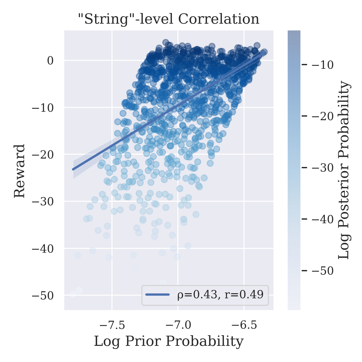
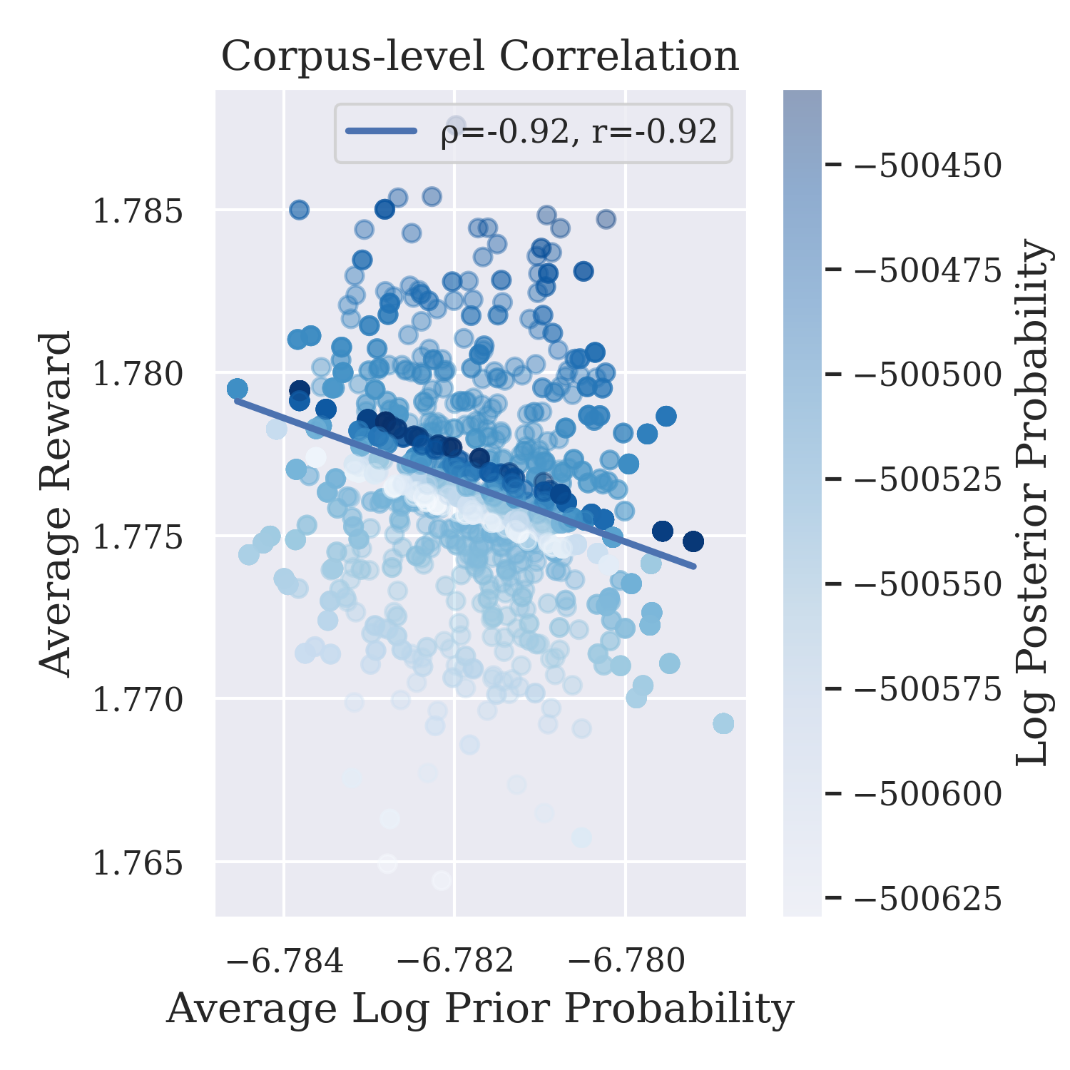
Figure 1: Illustration of the probability–quality trade-off with toy data, where quality is measured by the reward function. (Left) “String”-level correlations between probability and reward, where strings are mimicked by arbitrary objects. (Right) Corpus-level correlations between average log-probability and average reward. We include a best-fit line for corpora in the typical set, i.e., those with sample entropy close to ${\mathrm{H}}({{p}_{{\textsc{+}}}})$. In both figures, the log-probability of each string or corpus is coloured according to high (dark) and low (light).

The trade-off described in Prop. 1 fundamentally arises as a consequence of typicality and the fact that ${{p}_{{\textsc{+}}}}({\boldsymbol{y}})\propto{p}({\boldsymbol{y}})\big{(}\exp{{r}}({\boldsymbol{y}})\big{)}$. We aim to demonstrate these theoretical principles with an easily reproducible toy experiment, where we model these distributions over a finite set of objects ${x}\in{D}$. That is, we will show the existence of the trade-off using the toy models ${{p}_{{\textsc{+}}}}({x})$, ${p}({x})$ and ${{r}}({x})$.

Modeling ${{p}_{{\textsc{+}}}}$, ${p}$ and ${{r}}$.

We set $|{D}|=1,000$ and model ${{p}_{{\textsc{+}}}}({x})$ by sampling a distribution from the Dirichlet distribution. Then, we create the prior ${p}({x})$ by applying the softmax to a scaled and noised version of this distribution. That is, we define ${p}(\cdot)\mathrel{{\stackrel{{\scriptstyle\textnormal{def}}}{{=}}}}\mathrm{softmax}\big{(}{{p}_{{\textsc{+}}}}(\cdot)^{\frac{1}{{\tau}}}+\epsilon)\big{)}$ where $\epsilon\sim U(-\kappa,\kappa)$ and ${\tau}\in{\mathbbm{R}_{+}}$, $\kappa\in{\mathbbm{R}_{+}}$ are our hyperparameters. We then define ${{r}}({x})$ analogously to Eq. 4 with ${{r}}({x})=\log\frac{{{p}_{{\textsc{+}}}}({x})}{{p}({x})}$. The distributions of ${{p}_{{\textsc{+}}}}({x})$, ${p}({x})$ and ${{r}}({x})$ over the domain ${D}$ can be seen in App. F. To induce Simpson’s paradox, we tune $\kappa$ and ${\tau}$ such that they are positively correlated, shown in Fig. 1 on the left.

Constructing Corpora with Causal Bootstrapping.

An important point about the trade-off in Prop. 1 is that it occurs with high probability. To illustrate this, we use causal bootstrapping (Little and Badawy, 2020) to construct corpora that are uniformly distributed across 10 bands of average log-probability under the prior. Then, we compute and visualize the corpus probabilities, i.e., $\log{{p}_{{\textsc{+}}}}({\mathcal{X}})$ where ${\mathcal{X}}\mathrel{{\stackrel{{\scriptstyle\textnormal{def}}}{{=}}}}{\{{x}^{(n)}\}}_{n=1}^{N}$ denotes a corpus of toy objects. If Prop. 1 is correct, we expect to see that corpora exhibiting the trade-off have much higher probability than those that do not. We examine 1,000 corpora sampled this way, each with 100k samples.

6.2 The Trade-off in Practice

Here we demonstrate the existence of the probability–quality trade-off with an open-sourced aligned language model based on the Llama 2 family (Touvron et al., 2023). Using sampling adaptors we sample a corpus ${\mathcal{Y}}$ of 2,000 texts from an RLHF-tuned model ${q_{{\textsc{+}}}}$. Towards this, we randomly choose 1,000 prompts using the helpfulness dataset from Perez et al. (2022) and for each prompt, we produce two generations. Then, for every string in this corpus, we obtain its log-probability under the prior language model $\log{p}({\boldsymbol{y}})$ and its reward ${{r}}({\boldsymbol{y}})$. The prior and reward models are the same as those used to train ${q_{{\textsc{+}}}}$ in an RLHF scheme. We repeat this using five sampling adaptors at five temperatures, totaling 25 sampling schemes and thus $50,000$ $\big{(}\log{p}({\boldsymbol{y}}),{{r}}({\boldsymbol{y}})\big{)}$ pairs. To observe the trade-off, we compute the Pearson and Spearman’s correlation between $\log{p}({\boldsymbol{y}})$ and ${{r}}({\boldsymbol{y}})$ at the string level, and between $\frac{\log{p}({\mathcal{Y}})}{N}$ and $\frac{{{r}}({\mathcal{Y}})}{N}$ at the corpus level.

Resampling Corpora with the IMHA.

To compute corpus-level correlations we require a lot of data points of the average log-probability and average reward. However, because sampling multiple corpora is prohibitively expensive, we use the IMHA with standard bootstrap resampling (Bradley Efron, 1994) to create multiple corpora for each of the 25 sampling schemes. Given a corpus of strings generated from ${q_{{\textsc{+}}}}$ with a sampling adaptor ${\boldsymbol{\alpha}}$, we resample uniformly with replacement $N$ times, accepting and rejecting each as described in Algorithm 1. This gives us a resampled corpus ${\mathcal{Y}}^{\prime}$. Then, we compute the average log-likelihood $\frac{\log{p}({\mathcal{Y}}^{\prime})}{N}$ and average reward $\frac{{{r}}({\mathcal{Y}}^{\prime})}{N}$. We do this 2,000 times per sampling scheme, giving us a total of 50,000 $\left(\frac{\log{p}({\mathcal{Y}})}{N},\frac{{{r}}({\mathcal{Y}}^{\prime})}{N}\right)$ pairs, which we then use to we compute the corpus-level correlations. We set $N=200,000$ as preliminary experiments showed that for $N\geq 200,000$ the IMHA converges, i.e, the autocorrelation measured with Cramer’s V falls to $<0.10$.

Sampling Adaptors.

The five sampling adaptors we examine are: top-${k}$ sampling (Fan et al., 2018) for ${k}\in{\{30,50\}}$, nucleus sampling (Holtzman et al., 2020) for ${\pi}\in{\{0.90,0.95\}}$, $\eta$ sampling (Hewitt et al., 2022) and locally-typical sampling (Meister et al., 2023b). For each setting, we examine five temperatures ${\tau}\in{\{0.5,0.75,1.0,1.25,1.5\}}$. This gives us a total of 25 settings that cover various real-world use cases. As a baseline, we also include ancestral sampling.

Models.

We utilize the family of 7B reward, RLHF-tuned and prior language models from Rando and Tramèr (2024) based on Llama 2 7B (Touvron et al., 2023). Specifically, we use the baseline reward and RLHF-tuned models trained on the helpfulness dataset from Perez et al. (2022).

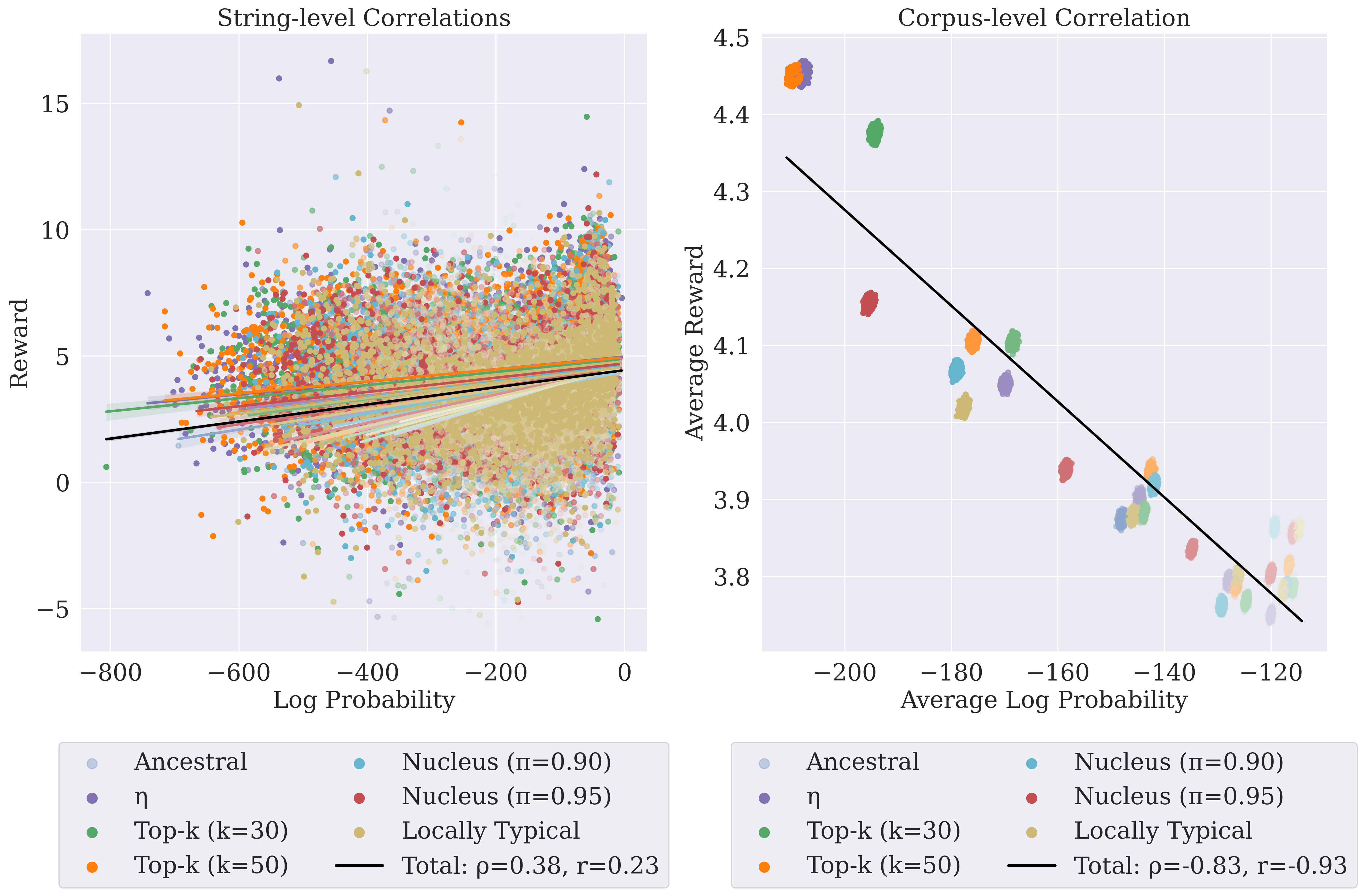
Figure 2: The probability–quality relationship, where quality is measured by the reward function. (Left) String-level correlations between log-probability and quality. (Right) Corpus-level correlations between average log-probability and average quality, with corpora created by different sampling adaptors. Higher intensity of the colours denote higher temperatures used with the sampling adaptor.

7 Results

Our results confirm our theoretical findings in § 5.

A Strong Anti-correlation.

In both toy and empirical settings, we observe at the corpus level a strong linear anti-correlation between the average log-probability $\frac{\log{p}({\mathcal{Y}})}{N}$ and reward $\frac{{{r}}({\mathcal{Y}})}{N}$. In the toy experiment, as shown in Fig. 1 corpora in the typical set have average log-probabilities and average rewards that exhibit a Pearson correlation of ${r}=-0.92$. And, importantly, these typical corpora occur with significantly higher probability than those that do not. For example, the median log-probability difference between a corpus in and out of the typical set is $10^{84}$ fold. The results in the empirical experiment with real language models are generally consistent with the toy experiment. We observe a Pearson correlation between the average log-probability and average reward of ${r}=-0.93$ with relatively few outliers.

Sampling Adaptors Control the Trade-off.

We observe in Fig. 2 that corpora sampled with different sampling adaptors are centered at different points on the trade-off and follow qualitatively expected trends. For example, corpora sampled with different temperatures have average log-probabilities that follow the expected order —high temperature corpora have lower average log-probabilities and higher average reward. And, at ${\tau}=1.0$ all sampling adaptors produce corpora with higher average log-probability and lower average reward than ancestral sampling. These results are expected since lower temperature and the examined sampling adaptors skew the sampling distribution towards high probability strings. The behaviour when comparing sampling adaptors with different degrees of truncation also follows expectations, e.g., corpora sampled with nucleus sampling for ${\pi}=0.95$ have lower average reward than those sampled with ${\pi}=0.90$. These findings are in line with our theoretical exposition in § 5.2 and suggest that we can use sampling adaptors to control the average reward of sampled corpora.

Simpson’s Paradox.

We observe in both toy (Fig. 1) and empirical data (Fig. 2) the emergence of Simpson’s paradox. At the string-level, we measure rank correlations of ${\rho}=0.43$ in the toy setting ${\rho}=0.38$ in the empirical setting. In the latter case, this positive correlation is probably explained by the fact that the reward model is trained to model preferences of helpfulness and the prior Llama 2 7B model has likely seen related texts in its training data. In both settings, we simultaneously find an anti-correlation at the corpus level between average log-probability and average reward. These results are consistent with our expectations in § 5.3—the reversal emerges because the trade-off arises out of typicality, independently of the true relationship between probability and quality at the string level.

8 Conclusion

Our work examines the relationship between probability and reward in sampling from RLHF-tuned language models. We have provided a formal argument and empirical evidence that there exists a trade-off between these two quantities when generating text at scale. Notably, this trade-off exists as a consequence of typicality, is independent of the relationship between reward and probability at the string level, and applies to any conditionally aligned language model, not just those aligned with RLHF. Moreover, we have uncovered a new role of sampling adaptors—the choice of sampling adaptor allows us to select how much likelihood we exchange for reward. This finding presents a new direction of research for improving reward alignment or mitigating reward overfitting in RLHF-tuned models, and the development of sampling adaptors for conditional text generation.

Limitations

There are three main limitations to our work. First, is that we only conduct empirical analysis for English and Transformer-based language models. Second, we don’t experiment over all sampling adaptors, e.g., we did not consider Mirostat-sampling (Basu et al., 2021) or contrastive search decoding (Su et al., 2022) in our experiments. These choices were made because the theory holds independently of these factors, though further work should consider other model architectures, sampling adaptors and models that span a variety of languages and domains. Finally, we have only examined the probability–quality relationship under the paradigm of RLHF (and equivalently, DPO, as we show in App. E), but not other alignment methods like ORPO (Hong et al., 2024) and KTO (Ethayarajh et al., 2024). We leave those to future work.

Ethics Statement

This paper provides a theoretical analysis of language models. To the best of the authors’ knowledge, this paper has no ethical implications.

Appendix A Supplementary proofs for § 5

A.1 Proof of Eq. 9

Proof.

$${\mathbb{P}}\left({\mathcal{Y}}\notin{T_{N}^{\varepsilon}}({q_{{\textsc{+}}}})\right) ={\mathbb{P}}(\Big{|}{\mathrm{H}}({\boldsymbol{Y}},{A}={\textsc{+}})+\frac{\log{q_{{\textsc{+}}}}({\mathcal{Y}})}{N}\Big{|}\geq\varepsilon)$$ (12a)

$$={\mathbb{P}}(\Big{|}{\mathrm{H}}({\boldsymbol{Y}},{A}={\textsc{+}})-\frac{-\log{q_{{\textsc{+}}}}({\mathcal{Y}})}{N}\Big{|}\geq\varepsilon)$$ (12b)

$$\leq\frac{{\mathbb{V}}(\frac{-\log{q_{{\textsc{+}}}}({\mathcal{Y}})}{N})}{\varepsilon^{2}}=\frac{{\mathbb{V}}(-\log{q_{{\textsc{+}}}}({\boldsymbol{y}}))}{N\varepsilon^{2}}=\frac{{\mathbb{V}}({I})}{N\varepsilon^{2}}$$ (12c)

Eq. 12c holds due to Chebyshev’s inequality. ∎

A.2 Proof of the Probability–Quality trade-off

Proof.

Consider the $(N,\varepsilon)$-typical set

$${T_{N}^{\varepsilon}}({q_{{\textsc{+}}}})\mathrel{{\stackrel{{\scriptstyle\textnormal{def}}}{{=}}}}\Big{\{}{\mathcal{Y}}\in({{{{\Sigma}}^{*}}})^{N}\mid\Big{|}{\mathrm{H}}({\boldsymbol{Y}},{A}={\textsc{+}})+\frac{\log{q_{{\textsc{+}}}}({\mathcal{Y}})}{N}\Big{|}<\varepsilon\Big{\}}$$ (13)

By rewriting Eq. 4

$$\frac{{{r}}({\boldsymbol{y}})}{\beta}=\log\frac{{q_{{\textsc{+}}}}({\boldsymbol{y}})}{{p}({\boldsymbol{y}})}+\log{{Z}({\textsc{+}})}$$

as

$$\log{q_{{\textsc{+}}}}({\boldsymbol{y}})=\frac{{{r}}({\boldsymbol{y}})}{\beta}+\log{p}({\boldsymbol{y}})-\log{{Z}({\textsc{+}})},$$

and summing over all ${\boldsymbol{y}}\in{\mathcal{Y}}$, we get

$$\log{q_{{\textsc{+}}}}({\mathcal{Y}})=\frac{{{r}}({\mathcal{Y}})}{\beta}+\log{p}({\mathcal{Y}})-N\log{{Z}({\textsc{+}})},$$ (14)

Substituting Eq. 14 into Eq. 10, we obtain

$${T_{N}^{\varepsilon}}({q_{{\textsc{+}}}}) =\Big{\{}{\mathcal{Y}}\in({{{{\Sigma}}^{*}}})^{N}\mid\Big{|}{\mathrm{H}}({\boldsymbol{Y}},{A}={\textsc{+}})+\frac{{{r}}({\mathcal{Y}})}{N\beta}+\frac{\log{p}({\mathcal{Y}})}{N}-\log{{Z}({\textsc{+}})}\Big{|}<\varepsilon\Big{\}}$$

$$=\Big{\{}{\mathcal{Y}}\in({{{{\Sigma}}^{*}}})^{N}\mid\Big{|}C+\frac{\log{p}({\mathcal{Y}})}{N}+\frac{{{r}}({\mathcal{Y}})}{N\beta}\Big{|}<\varepsilon\Big{\}}$$

Due to Chebyshev’s inequality, ${\mathbb{P}}\left({\mathcal{Y}}\notin T_{N}^{\varepsilon}({q_{{\textsc{+}}}})\right)\leq\frac{{\mathbb{V}}({I})}{N\varepsilon^{2}}$, we have $\Big{|}C+\frac{\log{p}({\mathcal{Y}})}{N}+\frac{{{r}}({\mathcal{Y}})}{N\beta}\Big{|}<\varepsilon$ with probability at least $\left(1-\frac{{\mathbb{V}}({I})}{N\varepsilon^{2}}\right)$ for all $N$ and $\varepsilon>0$. When $N\geq\frac{{\mathbb{V}}({I})}{\delta\varepsilon^{2}}$, the above holds with probability at least $(1-\delta)$.∎

Appendix B Infinite-Entropy Language Models

A key assumption we have made in this paper is that all language models ${p}$ under consideration have finite entropy. In general, this is not true. To make this point clear, we give an example of a simple language model whose entropy diverges.

Example 1 (A Tight LM with Infinite Entropy).

Let ${{\Sigma}}\mathrel{{\stackrel{{\scriptstyle\textnormal{def}}}{{=}}}}\{a\}$ and define for $t=1,2,\ldots$

$${p}(\underbrace{a\cdots a}_{\textnormal{$t$ times}})\mathrel{{\stackrel{{\scriptstyle\textnormal{def}}}{{=}}}}\frac{1}{\lg\left(t+1\right)}-\frac{1}{\lg\left(t+2\right)}.$$ (15)

Proposition 2.

The language model ${p}$ from Eq. 15 is tight and has infinite entropy.

Proof.

The proof follows Baer (2008). We consider the language model:

$${p}(\underbrace{a\cdots a}_{\textnormal{$t$ times}})\mathrel{{\stackrel{{\scriptstyle\textnormal{def}}}{{=}}}}\frac{1}{\lg\left(t+1\right)}-\frac{1}{\lg\left(t+2\right)}$$ (16)

${p}(\underbrace{a\cdots a}_{\textnormal{$t$ times}})$ is positive over $t=1,2,\ldots$ and sums to $1$ since it forms a telescoping sum with the only remaining term $\frac{1}{\lg\left(2\right)}=1$. This proves that ${p}$ is tight.

Furthermore, we can show that ${p}$’s entropy is $\infty$. Let us denote ${p}_{t}\mathrel{{\stackrel{{\scriptstyle\textnormal{def}}}{{=}}}}{p}(\underbrace{a\cdots a}_{\textnormal{$t$ times}})$, and begin by pointing out several facts. First, the monotonicity and convexity of $\frac{1}{\lg x}$ is easily seen by noting that its first derivative is $-\frac{1}{x\lg^{2}x\log 2}$ (negative for $x>1$) and its second derivative is $\frac{\lg(x+\frac{2}{\log 2})}{x^{2}\lg^{3}x\log(2)}$ (positive for $x>1$). This will allow us to bound ${p}_{t}$ from below with ${p}_{t}^{\prime}\mathrel{{\stackrel{{\scriptstyle\textnormal{def}}}{{=}}}}\frac{1}{t\lg^{2}t\log 2}$, which is monotonically decreasing and less than $\frac{1}{2}$ for $t\geq 3$. Then, we point out that with basic calculus we can see that ${p}\lg{p}$ is monotonically decreasing with ${p}$ for ${p}<\frac{1}{2}$. With these, we can say that ${p}_{t}^{\prime}\lg{p}_{t}^{\prime}$ is monotonically decreasing for $t\geq 2$ since ${p}_{t}^{\prime}<\frac{1}{2}$ for these $t$. We are now ready to lower bound ${\mathrm{H}}({p})$ with an expression equal to infinity, thereby showing that ${\mathrm{H}}({p})$ is infinite:

$${\mathrm{H}}\left({p}\right) =-\sum_{t=1}^{\infty}{p}_{t}\lg{p}_{t}$$ (17a)

$$=-{p}_{1}\lg{p}_{1}-{p}_{2}\lg{p}_{2}-\sum_{t=3}^{\infty}{p}_{t}\lg{p}_{t}$$ (17b)

$$=-{p}_{1}\lg{p}_{1}-{p}_{2}\lg{p}_{2}-\sum_{t=3}^{\infty}\left(\frac{1}{\lg\left(t+1\right)}-\frac{1}{\lg\left(t+2\right)}\right)\lg\left(\frac{1}{\lg\left(t+1\right)}-\frac{1}{\lg\left(t+2\right)}\right)$$ (17c)

$$>\frac{1}{\log 2}\sum^{\infty}_{t=3}\frac{1}{t\lg^{2}t}(\lg t+\lg\lg^{2}t+\lg\log 2)$$ (17d)

$$>\frac{1}{\log 2}\sum^{\infty}_{t=3}\frac{1}{t\lg^{2}t}$$ (17e)

$$>\frac{1}{\log 2}\int^{\infty}_{3}\frac{1}{t\lg t}dt$$ (17f)

$$>\lim_{n\rightarrow\infty}(\lg 2)(\lg\lg n-\lg\lg 3)=\infty$$ (17g)

∎

Appendix C A Tighter (Chernoff) Bound

In this section, we give a tighter concentration inequality than the (standard) one derived with Chebyshev’s inequality. The inequality displayed in Eq. 9 is weak in the sense that the average right hand size is ${\mathcal{O}}(\frac{1}{N})$—ideally, we desire a concentration inequality that is exponential, i.e., ${\mathcal{O}}(\exp(-cN))$ for some constant $c\in{\mathbbm{R}_{+}}$. To prove such a tighter concentration inequality, we define a class of language models that we term sub-exponential language models. We show that both classical $n$-gram language models as well as modern Transformer-based language models are sub-exponential under our definition. We further show that we can apply the Chernoff–Cramér method to argue that the sample entropy collapses around the mean exponentially quickly.

Before we delve into our derivation, we highlight what makes a direct application of a standard concentration bound, e.g., a Hoeffding bound, tricky. Consider a language model ${p}$ with support everywhere on ${{{{\Sigma}}^{*}}}$. Furthermore, consider an enumeration ${\{{\boldsymbol{y}}_{n}\}}_{n=1}^{\infty}$ of ${{{{\Sigma}}^{*}}}$ such that $n>m$ implies ${p}({\boldsymbol{y}}_{n})\leq{p}({\boldsymbol{y}}_{m})$. Observing the infinite sum $\sum_{n=1}^{\infty}{p}({\boldsymbol{y}}_{n})=1$ is convergent, we must have that ${p}({\boldsymbol{y}}_{n})\rightarrow 0$ as $n\rightarrow\infty$. It follows by the continuity of $\log$, that $-\log{p}({\boldsymbol{y}}_{n})\rightarrow\infty$ as $n\rightarrow\infty$. A simpler way of stating the above is that the random variable ${I}({\boldsymbol{y}})=-\log{p}({\boldsymbol{y}})$, distributed according to

$${\mathbb{P}}({I}={\iota})={\sum_{{\boldsymbol{y}}\in{{{{\Sigma}}^{*}}}}}{p}({\boldsymbol{y}}){\mathbbm{1}}\{{\iota}=-\log{p}({\boldsymbol{y}})\},$$ (18)

is unbounded.

C.1 Prerequisites

We will now introduce several definitions and prove several results.

Definition 1 (Non-trivial Language Model).

We call a language model over ${{\Sigma}}$ non-trivial if its support is an infinite subset of ${{{{\Sigma}}^{*}}}$.

Definition 2 (Rényi Entropy).

Let ${p}$ be a language model over ${{\Sigma}}$. The Rényi entropy of ${p}$ is defined as

$${{\mathrm{H}}_{{\gamma}}}({p})=\begin{cases}\frac{1}{1-{\gamma}}\log{\sum_{{\boldsymbol{y}}\in{{{{\Sigma}}^{*}}}}}{p}({\boldsymbol{y}})^{\gamma}&{\gamma}\in(0,1)\\ -{\sum_{{\boldsymbol{y}}\in{{{{\Sigma}}^{*}}}}}{p}({\boldsymbol{y}})\log{p}({\boldsymbol{y}})&{\gamma}=1\end{cases}$$

for ${\gamma}\in(0,1]$

Definition 3.

A language model ${p}$ is eos-bounded if there exists $c$ such that ${p}({\textsc{eos}}\mid{\boldsymbol{y}})>c>0$ for all ${\boldsymbol{y}}\in{{{{\Sigma}}^{*}}}$. In other words, ${p}({\boldsymbol{y}}\oplus{\textsc{eos}})\leq(1-c)^{|{\boldsymbol{y}}|}$ for all ${\boldsymbol{y}}\in{{{{\Sigma}}^{*}}}$.

Proposition 3.

Let ${p}$ be an eos-bounded language model. Then, ${{\mathrm{H}}_{{\gamma}}}({p})<+\infty$ for ${\gamma}\in(0,1]$.

Proof.

We divide the proof into two cases.

Case 1: ${\gamma}\in(0,1)$. Consider the following manipulation

$${\sum_{{\boldsymbol{y}}\in{{{{\Sigma}}^{*}}}}}{p}({\boldsymbol{y}})^{{\gamma}} =\sum_{n=0}^{\infty}\sum_{{\boldsymbol{y}}\in{{\Sigma}}^{n}}{p}({\boldsymbol{y}})^{{\gamma}}$$ (19a)

$$\leq\sum_{n=0}^{\infty}(1-c)^{n{\gamma}}$$ (19b)

$$=\sum_{n=0}^{\infty}\left[(1-c)^{{\gamma}}\right]^{n}$$ (19c)

$$=\frac{1}{1-(1-c)^{{\gamma}}}<+\infty$$ (19d)

The last inequality follows because $c\in(0,1)$, and, thus, we have $0<(1-c)^{{\gamma}}<1$ and, thus, the geometric sum converges.

Case 2: $\alpha=1$. In the case of $\alpha=1$, Rényi entropy entropy turns into Shannon entropy. Because $\log(\cdot)$ is concave, we have

$$-{\sum_{{\boldsymbol{y}}\in{{{{\Sigma}}^{*}}}}} {p}({\boldsymbol{y}})\log{p}({\boldsymbol{y}})=\log\prod_{{\boldsymbol{y}}\in{{{{\Sigma}}^{*}}}}\frac{1}{{p}({\boldsymbol{y}})^{{p}({\boldsymbol{y}})}}$$ (20a)

$$=2\log\prod_{{\boldsymbol{y}}\in{{{{\Sigma}}^{*}}}}\left(\frac{1}{{p}({\boldsymbol{y}})^{\frac{1}{2}}}\right)^{{p}({\boldsymbol{y}})}$$ (20b)

$$\leq 2\log\left({\sum_{{\boldsymbol{y}}\in{{{{\Sigma}}^{*}}}}}\frac{{p}({\boldsymbol{y}})}{{p}({\boldsymbol{y}})^{\frac{1}{2}}}\right)$$ (20c)

$$=2\log\left({\sum_{{\boldsymbol{y}}\in{{{{\Sigma}}^{*}}}}}{p}({\boldsymbol{y}})^{\frac{1}{2}}\right)$$ (20d)

$$={\mathrm{H}}_{\frac{1}{2}}({p})$$ (20e)

$$<+\infty$$ (20f)

Eq. 20c holds due to GM–AM inequality $\prod_{i}x_{i}^{p_{i}}\leq\sum_{i}p_{i}x_{i}$, when $\sum_{i}p_{i}=1$ and $x_{i}>0\ \forall i$.

∎

Corollary 1.

Let ${p}$ be a Transformer-based language model. Then, ${\mathrm{H}}_{{\gamma}}({p})<+\infty$ for ${\gamma}\in(0,1]$.

Proof.

This follows from the proof in Du et al. (Prop. 4.7 and Thm. 5.9, 2023) that Transformer-based LMs are eos-bounded. ∎

Corollary 2.

Let ${p}$ be a tight $n$-gram language model. Then, ${\mathrm{H}}_{{\gamma}}({p})<+\infty$ for ${\gamma}\in(0,1]$.

Proof.

Tight $n$-gram LMs are trivially are eos-bounded. ∎

Proposition 4.

Let ${p}$ be an eos-bounded language model. Then, over the interval $(0,1]$, ${\mathrm{H}}_{{\gamma}}({p})$ is monotonically decreasing in ${\gamma}$. Moreover, if ${p}$ is a non-trivial language model, then ${\mathrm{H}}_{{\gamma}}({p})$ is strictly monotonically decreasing in ${\gamma}$.

Proof.

$$\diff{{{\mathrm{H}}_{{\gamma}}}({p})}{{\gamma}}= \frac{1}{(1-{\gamma})^{2}}\log{\sum_{{\boldsymbol{y}}\in{{{{\Sigma}}^{*}}}}}{p}({\boldsymbol{y}})^{\gamma}+\frac{1}{1-{\gamma}}{\sum_{{\boldsymbol{y}}\in{{{{\Sigma}}^{*}}}}}\frac{{p}({\boldsymbol{y}})^{\gamma}\log{p}({\boldsymbol{y}})}{{\sum_{{{\boldsymbol{y}}^{\prime}}\in{{{{\Sigma}}^{*}}}}}{p}({{\boldsymbol{y}}^{\prime}})^{\gamma}}$$ (21a)

$$= \frac{1}{(1-{\gamma})^{2}}{\sum_{{\boldsymbol{y}}\in{{{{\Sigma}}^{*}}}}}z({\boldsymbol{y}})\left(\log{\sum_{{{\boldsymbol{y}}^{\prime}}\in{{{{\Sigma}}^{*}}}}}{p}({{\boldsymbol{y}}^{\prime}})^{\gamma}\right)+\frac{1}{(1-{\gamma})}{\sum_{{\boldsymbol{y}}\in{{{{\Sigma}}^{*}}}}}z({\boldsymbol{y}})\log{p}({\boldsymbol{y}})$$ (21b)

$$= \frac{1}{(1-{\gamma})^{2}}{\sum_{{\boldsymbol{y}}\in{{{{\Sigma}}^{*}}}}}z({\boldsymbol{y}})\left(\log{\sum_{{{\boldsymbol{y}}^{\prime}}\in{{{{\Sigma}}^{*}}}}}{p}({{\boldsymbol{y}}^{\prime}})^{\gamma}\right)+\frac{1}{(1-{\gamma})^{2}}{\sum_{{\boldsymbol{y}}\in{{{{\Sigma}}^{*}}}}}z({\boldsymbol{y}})\log{p}({\boldsymbol{y}})^{1-{\gamma}}$$ (21c)

$$= \frac{1}{(1-{\gamma})^{2}}{\sum_{{\boldsymbol{y}}\in{{{{\Sigma}}^{*}}}}}z({\boldsymbol{y}})\left(\log{\sum_{{{\boldsymbol{y}}^{\prime}}\in{{{{\Sigma}}^{*}}}}}{p}({{\boldsymbol{y}}^{\prime}})^{\gamma}+\log{p}({\boldsymbol{y}})^{1-{\gamma}}\right)$$ (21d)

$$= \frac{1}{(1-{\gamma})^{2}}{\sum_{{\boldsymbol{y}}\in{{{{\Sigma}}^{*}}}}}z({\boldsymbol{y}})\left(-\log\frac{{p}({\boldsymbol{y}})^{\gamma}}{{\sum_{{{\boldsymbol{y}}^{\prime}}\in{{{{\Sigma}}^{*}}}}}{p}({{\boldsymbol{y}}^{\prime}})^{\gamma}}+\log{p}({\boldsymbol{y}})\right)$$ (21e)

$$= \frac{1}{(1-{\gamma})^{2}}{\sum_{{\boldsymbol{y}}\in{{{{\Sigma}}^{*}}}}}z({\boldsymbol{y}})\log\frac{{p}({\boldsymbol{y}})}{z({\boldsymbol{y}})}$$ (21f)

$$= -\frac{1}{(1-{\gamma})^{2}}{\mathrm{KL}}(z\,\|\,{p})\leq 0$$ (21g)

where $z({\boldsymbol{y}})\mathrel{{\stackrel{{\scriptstyle\textnormal{def}}}{{=}}}}\frac{{p}({\boldsymbol{y}})^{\gamma}}{{\sum_{{\boldsymbol{y}}\in{{{{\Sigma}}^{*}}}}}{p}({\boldsymbol{y}})^{\gamma}}$. Because the derivative of ${{\mathrm{H}}_{{\gamma}}}({p})$ with regard to ${\gamma}$ is $\leq$ 0 on the interval $(0,1]$, ${{\mathrm{H}}_{{\gamma}}}({p})$ is monotonically decreasing in ${\gamma}$. Moreover, when ${p}$ is non-trivial, which implies ${p}$ is not uniform nor a point mass, we have $z\neq{p},\forall{\gamma}\in(0,1)$. Thus $\diff{{{\mathrm{H}}_{{\gamma}}}({p})}{{\gamma}}=-\frac{1}{(1-{\gamma})^{2}}{\mathrm{KL}}(z\,\|\,{p})<0$, i.e., ${{\mathrm{H}}_{{\gamma}}}({p})$ is strictly monotonically decreasing on $(0,1)$. ∎

Proposition 5.

Let ${p}$ be an eos-bounded language model. Then, ${\mathbb{V}}({I})$ is finite.

Proof.

We show that ${\mathbb{V}}({I})$ is bounded for eos-bounded language models. Let $M\mathrel{{\stackrel{{\scriptstyle\textnormal{def}}}{{=}}}}{\sum_{{\boldsymbol{y}}\in{{{{\Sigma}}^{*}}}}}{p}({\boldsymbol{y}})^{\frac{1}{2}},z({\boldsymbol{y}})\mathrel{{\stackrel{{\scriptstyle\textnormal{def}}}{{=}}}}\frac{{p}({\boldsymbol{y}})^{\frac{1}{2}}}{M}$. Note that $M=\exp(\frac{1}{2}{\mathrm{H}}_{\frac{1}{2}}(p))<\infty$ due to Prop. 3. Then, we have

$${\mathbb{V}}({I}) ={\sum_{{\boldsymbol{y}}\in{{{{\Sigma}}^{*}}}}}{p}({\boldsymbol{y}})\left(\log\frac{1}{{p}({\boldsymbol{y}})}\right)^{2}-{\mathrm{H}}({p})^{2}$$ (22a)

$$\leq\left({\sum_{{\boldsymbol{y}}\in{{{{\Sigma}}^{*}}}}}{p}({\boldsymbol{y}})^{\frac{1}{2}}\log\frac{1}{{p}({\boldsymbol{y}})}\right)^{2}-{\mathrm{H}}({p})^{2}$$ (22b)

$$=\left(2{\sum_{{\boldsymbol{y}}\in{{{{\Sigma}}^{*}}}}}{p}({\boldsymbol{y}})^{\frac{1}{2}}\log\left(\frac{1}{{p}({\boldsymbol{y}})}\right)^{\frac{1}{2}}\right)^{2}-{\mathrm{H}}({p})^{2}$$ (22c)

$$=\left(2{\sum_{{\boldsymbol{y}}\in{{{{\Sigma}}^{*}}}}}Mz({\boldsymbol{y}})\log\frac{1}{Mz({\boldsymbol{y}})}\right)^{2}-{\mathrm{H}}({p})^{2}$$ (22d)

$$=\left(-2M\log M+2{\sum_{{\boldsymbol{y}}\in{{{{\Sigma}}^{*}}}}}Mz({\boldsymbol{y}})\log\frac{1}{z({\boldsymbol{y}})}\right)^{2}-{\mathrm{H}}({p})^{2}$$ (22e)

$$=\left(-2M\log M+2M{\mathrm{H}}_{1}(z)\right)^{2}-{\mathrm{H}}({p})^{2}$$ (22f)

$$\leq\left(|2M\log M|+|2M{\mathrm{H}}_{1/2}(z)|\right)^{2}-{\mathrm{H}}({p})^{2}\qquad\text{(monotonicity of Rényi Entropy)}$$ (22g)

$$=\left(2M\log M+4M\log\left({\sum_{{\boldsymbol{y}}\in{{{{\Sigma}}^{*}}}}}z({\boldsymbol{y}})^{1/2}\right)\right)^{2}-{\mathrm{H}}({p})^{2}$$ (22h)

$$=\left(2M\log M+4M\left(\frac{3}{4}{\mathrm{H}}_{1/4}(p)-\frac{1}{2}\log M\right)\right)^{2}-{\mathrm{H}}({p})^{2}$$ (22i)

$$<+\infty$$ (22j)

∎

Definition 4 (Rényi Gap).

Let ${p}$ be a language model and let ${\gamma}\in(0,1]$. The Rényi gap is defined as

$${{\Delta}{\gamma}}({p})={{\mathrm{H}}_{{\gamma}}}({p})-{\mathrm{H}}({p})$$ (23)

Corollary 3.

Let ${p}$ be a language model and let $\alpha\in(0,1]$. Then, the Rényi gap ${{\Delta}{\gamma}}({p})$ is non-negative.

Proof.

This follows from Prop. 4. ∎

Lemma 1.

Let ${p}$ be a non-trivial, eos-bounded language model. Then, for any $\varepsilon>0$, there exists an ${\gamma}\in(0,1)$ such that the Rényi gap $0<{{\Delta}{\gamma}}<\varepsilon$.

Proof.

This follows from the ${{\Delta}{\gamma}}$ being a continuous monotonically decreasing function in ${\gamma}$ and ${{\Delta}{\gamma}}=0$ when ${\gamma}=1$. ∎

C.2 A Tighter Concentration Bound

We now introduce a sharper version of the AEP for eos-bounded language models. As shown in Corollary 1, this includes Transformer-based language models, which constitute the base architecture for most modern models (Brown et al., 2020; Touvron et al., 2023). The theorem is stated below.

Theorem 2.

Let ${p}$ be an eos-bounded, non-trivial language model. Then, there exists a function $s(\varepsilon)>0$ such that, for any $\varepsilon>0$, we have

$${\mathbb{P}}\left(\left|\frac{1}{N}\sum_{n=1}^{N}{I}_{n}-{\mathrm{H}}({p})\right|\geq\varepsilon\right)\leq 2\exp(-s(\varepsilon)N)$$ (24)

with

$$s(\varepsilon)\mathrel{{\stackrel{{\scriptstyle\textnormal{def}}}{{=}}}}-t(\varepsilon)({\Delta}_{1-t(\varepsilon)}({p})-\varepsilon)$$ (25)

Proof.

To prove the result, we apply a Chernoff bound. This is a one-sided bound and the other will follow by symmetry.

$${\mathbb{P}}\left(\frac{1}{N}\sum_{n=1}^{N}{I}_{n}-{\mathrm{H}}({p})\geq\varepsilon\right) \leq\inf_{t>0}\exp(-t\varepsilon)\operatorname*{{\mathbb{E}}}\prod_{n=1}^{N}\exp\left(\frac{t}{N}({I}_{n}-{\mathrm{H}}({p}))\right)$$ (26a)

$$=\inf_{t>0}\exp(-t\varepsilon)\exp(-t{\mathrm{H}}({p}))\operatorname*{{\mathbb{E}}}\prod_{n=1}^{N}\exp\left(\frac{t}{N}{I}_{n}\right)$$ (26b)

$$=\inf_{t>0}\exp(-t\varepsilon)\exp(-t{\mathrm{H}}({p}))\prod_{n=1}^{N}\operatorname*{{\mathbb{E}}}\exp\left(\frac{t}{N}{I}_{n}\right)$$ (26c)

$$=\inf_{t>0}\exp(-t\varepsilon)\exp(-t{\mathrm{H}}({p}))\prod_{n=1}^{N}{\sum_{{\boldsymbol{y}}\in{{{{\Sigma}}^{*}}}}}{p}({\boldsymbol{y}})\exp\left(-\frac{t}{N}\log{p}({\boldsymbol{y}})\right)$$ (26d)

$$=\inf_{t>0}\exp(-t\varepsilon)\exp(-t{\mathrm{H}}({p}))\prod_{n=1}^{N}{\sum_{{\boldsymbol{y}}\in{{{{\Sigma}}^{*}}}}}{p}({\boldsymbol{y}})^{1-\frac{t}{N}}$$ (26e)

$$=\inf_{t>0}\exp(-t\varepsilon)\exp(-t{\mathrm{H}}({p}))\prod_{n=1}^{N}\exp\left(\frac{t}{N}{\mathrm{H}}_{1-\frac{t}{N}}({p})\right)$$ (26f)

$$=\inf_{t>0}\exp(-t\varepsilon)\exp(-t{\mathrm{H}}({p}))\exp\left(t{\mathrm{H}}_{1-\frac{t}{N}}({p})\right)$$ (26g)

$$=\inf_{t>0}\exp(-t\varepsilon)\exp(t({\mathrm{H}}_{1-\frac{t}{N}}({p})-{\mathrm{H}}({p})))$$ (26h)

$$=\inf_{t>0}\exp(-t\varepsilon)\exp(t({\Delta}_{1-\frac{t}{N}}({p})))$$ (26i)

$$=\inf_{t>0}\exp\left(t({\Delta}_{1-\frac{t}{N}}({p})-\varepsilon)\right)$$ (26j)

$$=\inf_{t^{\prime}>0}\exp\left(Nt^{\prime}({\Delta}_{1-t^{\prime}}({p})-\varepsilon)\right)$$ (26k)

Now, by Lemma 1, for any $\epsilon>0$ we can find a $0<t(\varepsilon)<1$ such that ${\Delta}_{1-t(\varepsilon)}({p})-\varepsilon<0$. Thus, we have

$${\mathbb{P}}\left(\frac{1}{N}\sum_{n=1}^{N}{I}_{n}-{\mathrm{H}}({p})\geq\varepsilon\right)\leq\exp(Nt(\varepsilon)({\Delta}_{1-t(\varepsilon)}({p})-\varepsilon)).$$ (27)

Similarly, we have:

$${\mathbb{P}}\left(\frac{1}{N}\sum_{n=1}^{N}{I}_{n}-{\mathrm{H}}({p})\leq-\varepsilon\right)\leq\exp(Nt(\varepsilon)(-{\Delta}_{1-t(\varepsilon)}({p})-\varepsilon))\leq\exp(Nt(\varepsilon)({\Delta}_{1-t(\varepsilon)}({p})-\varepsilon))$$ (28)

And, finally, we get:

$${\mathbb{P}}\left(\left|\frac{1}{N}\sum_{n=1}^{N}{I}_{n}-{\mathrm{H}}({p})\right|\geq\varepsilon\right) \leq{\mathbb{P}}\left(\frac{1}{N}\sum_{n=1}^{N}{I}_{n}-{\mathrm{H}}({p})\geq\varepsilon\right)+{\mathbb{P}}\left(\frac{1}{N}\sum_{n=1}^{N}{I}_{n}-{\mathrm{H}}({p})\leq-\varepsilon\right)$$

$$\leq 2\exp(Nt(\varepsilon)({\Delta}_{1-t(\varepsilon)}({p})-\varepsilon)).$$ (29)

Substituting in $s(\varepsilon)=-t(\varepsilon)({\Delta}_{1-t(\varepsilon)}({p})-\varepsilon)>0$, we arrive at

$${\mathbb{P}}\left(\left|\frac{1}{N}\sum_{n=1}^{N}{I}_{n}-{\mathrm{H}}({p})\right|\geq\varepsilon\right)\leq 2\exp(-s(\varepsilon)N),$$ (30)

which tends to $0$ exponentially quickly as $N\rightarrow\infty$. Note that $2\exp(-s(\varepsilon)N)$ is ${\mathcal{O}}(\exp(-cN))$ for $c=s(\varepsilon)$, which proves the result. ∎

In words, with respect to Transformer-based language models, Theorem 2 says that if we have a model ${p}$ and randomly sample $N$ strings ${\mathcal{Y}}\sim{p}$, when we average their surprisal values we approach the entropy of ${p}$ exponentially quickly. One caveat is that the constant in the exponential is not a universal constant, i.e., it depends on $\varepsilon$. This is less desirable, of course, but it is an improvement over the ${\mathcal{O}}(\frac{1}{N})$ rate given by an application of the standard AEP. We leave finding a universal constant for eos-bounded language models to future work.

Appendix D Sampling Adaptors and String Probability

In this section our goal is to show that using a sampling adaptor ${\boldsymbol{\alpha}}$ modifies string probability under the prior ${p}({\boldsymbol{y}})$ without modifying the likelihood of alignment with preferences ${p}({A}={\textsc{+}}\mid{\boldsymbol{y}})$. Let us begin by decomposing a sampling adaptor into its constitutent components. Inspired by Meister et al. (2023a), we note that most sampling adaptors can be formulated as the composition of truncation and scaling functions. The truncation function ${C}\colon{{{{\Sigma}}^{*}}}\rightarrow{\mathcal{P}}({\overline{{{\Sigma}}}})$ is a function used to find the set of tokens that meets specified criteria given the prior context, so that tokens deemed likely to lead to undesirable text can have their probability reassigned to other tokens, e.g., to only keep the top-${k}$ tokens. The scaling function ${f}\colon{\mathbbm{R}}\rightarrow{\mathbbm{R}}$ is a simple scaling of the token probability, e.g., scaling the probability by $\frac{1}{{\tau}}$ for some temperature parameter ${\tau}\in{\mathbbm{R}_{+}}$. With these definitions we can express a sampling adaptor ${\boldsymbol{\alpha}}$ as:

$${\boldsymbol{\alpha}}\left({p}(\cdot\mid{{\boldsymbol{y}}_{<t}})\right)({y})={f}({p}({y}\mid{{\boldsymbol{y}}_{<t}})){\mathbbm{1}}{\{{y}\in{{C}\left({p}(\cdot\mid{{\boldsymbol{y}}_{<t}})\right)}\}}$$ (31)

That is, given a token distribution ${p}(\cdot\mid{{\boldsymbol{y}}_{<t}})$, we apply the scaling function to scale token probabilities as needed and then remove tokens according to the truncation function to arrive at the output unnormalized distribution. For instance, we can express nucleus sampling (Holtzman et al., 2020) with:

$${f}_{\mathrm{nucleus}}\big{(}({p}({y}\mid{{\boldsymbol{y}}_{<t}})\big{)} ={\mathbb{I}}\big{(}{p}({y}\mid{{\boldsymbol{y}}_{<t}})\big{)}$$ (32a)

$${C}_{\mathrm{nucleus}}\big{(}({p}({y}\mid{{\boldsymbol{y}}_{<t}})\big{)} =\operatorname*{{argmin}}_{{\overline{{{\Sigma}}}}^{\prime}\subseteq{\overline{{{\Sigma}}}}}|{\overline{{{\Sigma}}}}^{\prime}|\qquad s.t.\sum_{{y}\in{\overline{{{\Sigma}}}}^{\prime}}{p}({y}\mid{{\boldsymbol{y}}_{<t}})\geq{\pi}$$ (32b)

where ${\mathbb{I}}$ denotes the identity function and ${\pi}\in{\mathbbm{R}_{+}}$ is a hyperparameter. See § D.1 for more examples. Now, let us consider the probability of a string under the resultant distribution ${{\tilde{{p}}}_{+}}$ when a sampling adaptor ${\boldsymbol{\alpha}}$ is used with an aligned model ${{p}_{{\textsc{+}}}}$. If also apply Bayes’ rule, with some rearrangement we have:

$${{\tilde{{p}}}_{+}}({\boldsymbol{y}}) ={\boldsymbol{\alpha}}\big{(}{{p}_{{\textsc{+}}}}(\cdot\mid{\boldsymbol{y}})\big{)}({\textsc{eos}})\prod_{t=1}^{|{\boldsymbol{y}}|}{\boldsymbol{\alpha}}\big{(}{{p}_{{\textsc{+}}}}(\cdot\mid{\boldsymbol{y}})\big{)}({{y}_{t}})$$

$$=\frac{\left({\mathbbm{1}}{\{{\textsc{eos}}\in{{C}_{\boldsymbol{y}}}\}}\prod_{t=1}^{|{\boldsymbol{y}}|}{\mathbbm{1}}{\{{{y}_{t}}\in{{C}_{t}}\}}\right)\left({f}\big{(}{p}({\textsc{eos}}\mid{\boldsymbol{y}})\big{)}\prod_{t=1}^{|{\boldsymbol{y}}|}{f}\big{(}{p}({{y}_{t}}\mid{{\boldsymbol{y}}_{<t}},{A}={\textsc{+}})\big{)}\right)}{{{Z}_{\boldsymbol{\alpha}}({\boldsymbol{y}})}}$$ (33a)

$$\propto\left({\mathbbm{1}}{\{{\textsc{eos}}\in{{C}_{\boldsymbol{y}}}\}}\prod_{t=1}^{|{\boldsymbol{y}}|}{\mathbbm{1}}{\{{{y}_{t}}\in{{C}_{t}}\}}\right)\left({p}({\textsc{eos}}\mid{\boldsymbol{y}})\prod_{t=1}^{|{\boldsymbol{y}}|}{p}({{y}_{t}}\mid{{\boldsymbol{y}}_{<t}}\right){p}({A}={\textsc{+}}\mid{\boldsymbol{y}})$$ (33b)

$$=\underbrace{{p}({\textsc{eos}}\mid{\boldsymbol{y}}){\mathbbm{1}}{\{{\textsc{eos}}\in{{C}_{\boldsymbol{y}}}\}}\prod_{t=1}^{|{\boldsymbol{y}}|}{p}({\textsc{eos}}\mid{{\boldsymbol{y}}_{<t}}){\mathbbm{1}}{\{{{y}_{t}}\in{{C}_{t}}\}}}_{\text{Modified Prior}}{p}({A}={\textsc{+}}\mid{\boldsymbol{y}})$$ (33c)

where we use the shorthands ${{C}_{t}}\mathrel{{\stackrel{{\scriptstyle\textnormal{def}}}{{=}}}}{{C}\left({p}(\cdot\mid{{\boldsymbol{y}}_{<t}})\right)}$ and ${{C}_{\boldsymbol{y}}}\mathrel{{\stackrel{{\scriptstyle\textnormal{def}}}{{=}}}}{{C}\left({p}(\cdot\mid{\boldsymbol{y}})\right)}$. What Eq. 33 says is that by decomposing a sampling adaptor into its constituent components, we find that we can can factorize out its effects and push them entirely to the prior. As a result, sampling adaptors that can be expressed this way—such as those in § D.1—can be used to control a string’s probability under the prior without affecting its likelihood of alignment with human preferences.

D.1 Examples of Sampling Adaptors

We note that these largely correspond to the examples in Meister et al. (2023a).

Example 2.

We recover ancestral sampling when ${f}(\cdot)={\mathbb{I}}(\cdot)$ and ${{C}\left({p}(\cdot\mid{{\boldsymbol{y}}_{<t}})\right)}={\overline{{{\Sigma}}}}$.

Example 3.

We recover temperature sampling when ${f}({p}({{y}_{t}}\mid{{\boldsymbol{y}}_{<t}}))\propto{p}({{y}_{t}}\mid{{\boldsymbol{y}}_{<t}})^{\frac{1}{{\tau}}}$ and ${{C}\left({p}(\cdot\mid{{\boldsymbol{y}}_{<t}})\right)}={\overline{{{\Sigma}}}}$.

Example 4.

We recover top-${k}$ sampling (Fan et al., 2018) when ${f}(\cdot)={\mathbb{I}}(\cdot)$ and

$${{C}\left({p}(\cdot\mid{{\boldsymbol{y}}_{<t}})\right)}=\operatorname*{{argmax}}_{{\overline{{{\Sigma}}}}^{\prime}\subseteq{\overline{{{\Sigma}}}}}\sum_{{y}\in{\overline{{{\Sigma}}}}^{\prime}}{p}({y}\mid{{\boldsymbol{y}}_{<t}})\qquad s.t.\,|{\overline{{{\Sigma}}}}^{\prime}|={k}$$ (34)

i.e., the set of top-${k}$ most probable tokens.

Example 5.

We recover locally typical sampling (Meister et al., 2023b) when when ${f}(\cdot)={\mathbb{I}}(\cdot)$ and

$${{C}\left({p}(\cdot\mid{{\boldsymbol{y}}_{<t}})\right)}=\operatorname*{{argmin}}_{{\overline{{{\Sigma}}}}^{\prime}\subseteq{\overline{{{\Sigma}}}}}\sum_{{y}\in{\overline{{{\Sigma}}}}^{\prime}}\big{|}{\mathrm{H}}({p}(\cdot\mid{{\boldsymbol{y}}_{<t}}))+\log{p}({y}\mid{{\boldsymbol{y}}_{<t}})\big{|}\qquad s.t.\,\sum_{{y}\in{\overline{{{\Sigma}}}}^{\prime}}{p}({y}\mid{{\boldsymbol{y}}_{<t}})\geq{\pi}$$ (35)

i.e., the set of items with log-probability closest to the token-level entropy that collectively have probability mass $\geq{\pi}$.

Example 6.

We recover $\eta$-sampling (Hewitt et al., 2022) when ${f}(\cdot)={\mathbb{I}}(\cdot)$ and

$${{C}\left({p}(\cdot\mid{{\boldsymbol{y}}_{<t}})\right)}={\{{y}\in{\overline{{{\Sigma}}}}\mid{p}({y}\mid{{\boldsymbol{y}}_{<t}})>\eta\}}$$ (36)

that is, the set of tokens with probability greater than $\eta$, where $\eta=\min(\epsilon,\sqrt{\epsilon}\exp(-{\mathrm{H}}({p}(\cdot\mid{{\boldsymbol{y}}_{<t}})))))$.

Appendix E The trade-off in DPO-aligned models

The probability–quality trade-off also applies to models aligned with direct preference optimization (DPO; Rafailov et al., 2023). Though an explicit reward function is not needed to train a language model with DPO, the training scheme maximises the same backward KL divergence objective as RLHF (Eq. 3; Korbak et al., 2023; Rafailov et al., 2023; Azar et al., 2023). We should thus expect that Prop. 1 applies to these models and observe the trade-off when we construct a reward function ${{r}}_{q_{{\textsc{+}}}}$ using the prior ${p}$ and aligned model ${q_{{\textsc{+}}}}$ as in Eq. 4. We employ the same setup as in § 6.2.

Models.

We use the 7B DPO-aligned and prior language models from Lee et al. (2024), both of which are based on Mistral 7B v0.2 (Jiang et al., 2023). The DPO-aligned model is fine-tuned on the Multifaceted Collection (Lee et al., 2024), a dataset with 192k samples capturing preferences of style (e.g., clarity, tone), informativeness, and harmlessness, among others. We construct the “secret” reward function as ${{r}}_{q_{{\textsc{+}}}}({\boldsymbol{y}})=\frac{{q_{{\textsc{+}}}}({\boldsymbol{y}})}{{p}({\boldsymbol{y}})}$, omitting the constant term.

Results.

We observe results identical to the setting with RLHF-tuned models. Specifically, we observe a strong anti-correlation (Pearson correlation of ${r}=-0.97$), trade-off control using sampling adaptors, and the emergence of Simpson’s paradox. These are expected since RLHF and DPO have the same minimization objective, thus supporting our formal arguments in § 5.

Figure 3: The probability–quality relationship in DPO-tuned models, where quality is measured by the secret reward function. (Left) String-level correlations between log-probability and quality. (Right) Corpus-level correlations between average log-probability and average quality, with corpora created by different sampling adaptors. Higher intensity of the colours denote higher temperatures used with the sampling adaptor.

Appendix F Toy Experiment Distributions

Figure 4: Toy models of ${{p}_{{\textsc{+}}}}({x})$, ${p}({x})$ and ${{r}}({x})$ analogous to the distributions over strings.

References

- Azar et al. (2023) Mohammad Gheshlaghi Azar, Mark Rowland, Bilal Piot, Daniel Guo, Daniele Calandriello, Michal Valko, and Rémi Munos. 2023. A general theoretical paradigm to understand learning from human preferences. arXiv preprint arXiv:2310.12036.
- Baer (2008) Michael Baer. 2008. A simple countable infinite-entropy distribution.
- Banchs et al. (2015) Rafael E. Banchs, L. F. D’Haro, and Haizhou Li. 2015. Adequacy–fluency metrics: Evaluating mt in the continuous space model framework. IEEE/ACM Transactions on Audio, Speech, and Language Processing, 23:472–482.
- Basu et al. (2021) Sourya Basu, Govardana Sachitanandam Ramachandran, Nitish Shirish Keskar, and Lav R. Varshney. 2021. Mirostat: a neural text decoding algorithm that directly controls perplexity. In International Conference on Learning Representations.
- Bradley and Terry (1952) Ralph Allan Bradley and Milton E. Terry. 1952. Rank analysis of incomplete block designs: I. the method of paired comparisons. Biometrika, 39:324.
- Bradley Efron (1994) R.J. Tibshirani Bradley Efron. 1994. An Introduction to the Bootstrap (1st ed.). Chapman and Hall/CRC.
- Brown et al. (2020) Tom Brown, Benjamin Mann, Nick Ryder, Melanie Subbiah, Jared D Kaplan, Prafulla Dhariwal, Arvind Neelakantan, Pranav Shyam, Girish Sastry, Amanda Askell, Sandhini Agarwal, Ariel Herbert-Voss, Gretchen Krueger, Tom Henighan, Rewon Child, Aditya Ramesh, Daniel Ziegler, Jeffrey Wu, Clemens Winter, Chris Hesse, Mark Chen, Eric Sigler, Mateusz Litwin, Scott Gray, Benjamin Chess, Jack Clark, Christopher Berner, Sam McCandlish, Alec Radford, Ilya Sutskever, and Dario Amodei. 2020. Language models are few-shot learners. In Advances in Neural Information Processing Systems, volume 33, pages 1877–1901. Curran Associates, Inc.
- Callison-Burch et al. (2007) Chris Callison-Burch, Cameron Fordyce, Philipp Koehn, Christof Monz, and Josh Schroeder. 2007. (meta-) evaluation of machine translation. In Proceedings of the Second Workshop on Statistical Machine Translation, pages 136–158, Prague, Czech Republic. Association for Computational Linguistics.
- Cover and Thomas (2006) Thomas M. Cover and Joy A. Thomas. 2006. Elements of Information Theory (Wiley Series in Telecommunications and Signal Processing). Wiley-Interscience, USA.
- Deonovic and Smith (2017) Benjamin E. Deonovic and Brian J. Smith. 2017. Convergence diagnostics for MCM draws of a categorical variable. arXiv preprint arXiv:1706.04919.
- Devlin et al. (2019) Jacob Devlin, Ming-Wei Chang, Kenton Lee, and Kristina Toutanova. 2019. BERT: Pre-training of deep bidirectional transformers for language understanding. In North American Chapter of the Association for Computational Linguistics.
- Djolonga et al. (2020) Josip Djolonga, Mario Lucic, Marco Cuturi, Olivier Bachem, Olivier Bousquet, and Sylvain Gelly. 2020. Precision-recall curves using information divergence frontiers. In Proceedings of the Twenty Third International Conference on Artificial Intelligence and Statistics, volume 108 of Proceedings of Machine Learning Research, pages 2550–2559. PMLR.
- Du et al. (2023) Li Du, Lucas Torroba Hennigen, Tiago Pimentel, Clara Meister, Jason Eisner, and Ryan Cotterell. 2023. A measure-theoretic characterization of tight language models. In Proceedings of the 61st Annual Meeting of the Association for Computational Linguistics (Volume 1: Long Papers), pages 9744–9770, Toronto, Canada. Association for Computational Linguistics.
- Ethayarajh et al. (2022) Kawin Ethayarajh, Yejin Choi, and Swabha Swayamdipta. 2022. Understanding dataset difficulty with -usable information. In Proceedings of the 39th International Conference on Machine Learning, volume 162 of Proceedings of Machine Learning Research, pages 5988–6008. PMLR.
- Ethayarajh et al. (2024) Kawin Ethayarajh, Winnie Xu, Niklas Muennighoff, Dan Jurafsky, and Douwe Kiela. 2024. Kto: Model alignment as prospect theoretic optimization. arXiv preprint arXiv:2402.01306.
- Fan et al. (2018) Angela Fan, Mike Lewis, and Yann Dauphin. 2018. Hierarchical neural story generation. In Proceedings of the 56th Annual Meeting of the Association for Computational Linguistics (Volume 1: Long Papers), pages 889–898, Melbourne, Australia. Association for Computational Linguistics.
- Fradelizi et al. (2016) Matthieu Fradelizi, Mokshay Madiman, and Liyao Wang. 2016. Optimal concentration of information content for log-concave densities. In High Dimensional Probability VII, pages 45–60, Cham. Springer International Publishing.
- Gao et al. (2023) Leo Gao, John Schulman, and Jacob Hilton. 2023. Scaling laws for reward model overoptimization. In Proceedings of the 40th International Conference on Machine Learning, volume 202 of Proceedings of Machine Learning Research, pages 10835–10866. PMLR.
- Hastings (1970) W. K. Hastings. 1970. Monte Carlo sampling methods using Markov chains and their applications. Biometrika, 57(1):97–109.
- He et al. (2024) Zhiwei He, Xing Wang, Wenxiang Jiao, Zhuosheng Zhang, Rui Wang, Shuming Shi, and Zhaopeng Tu. 2024. Improving machine translation with human feedback: An exploration of quality estimation as a reward model. arXiv preprint arXiv:2401.12873.
- Hewitt et al. (2022) John Hewitt, Christopher Manning, and Percy Liang. 2022. Truncation sampling as language model desmoothing. In Findings of the Association for Computational Linguistics: EMNLP 2022, pages 3414–3427, Abu Dhabi, United Arab Emirates. Association for Computational Linguistics.
- Holtzman et al. (2020) Ari Holtzman, Jan Buys, Li Du, Maxwell Forbes, and Yejin Choi. 2020. The curious case of neural text degeneration. In International Conference on Learning Representations.
- Hong et al. (2024) Jiwoo Hong, Noah Lee, and James Thorne. 2024. Orpo: Monolithic preference optimization without reference model. arXiv preprint arXiv:2403.07691.
- Hu et al. (2017) Zhiting Hu, Zichao Yang, Xiaodan Liang, Ruslan Salakhutdinov, and Eric P. Xing. 2017. Toward controlled generation of text. In Proceedings of the 34th International Conference on Machine Learning, volume 70 of Proceedings of Machine Learning Research, pages 1587–1596. PMLR.
- Ialongo (2016) Cristiano Ialongo. 2016. Understanding the effect size and its measures. Biochem Med (Zagreb).
- Jiang et al. (2023) Albert Q. Jiang, Alexandre Sablayrolles, Arthur Mensch, Chris Bamford, Devendra Singh Chaplot, Diego de las Casas, Florian Bressand, Gianna Lengyel, Guillaume Lample, Lucile Saulnier, Lélio Renard Lavaud, Marie-Anne Lachaux, Pierre Stock, Teven Le Scao, Thibaut Lavril, Thomas Wang, Timothée Lacroix, and William El Sayed. 2023. Mistral 7b. arXiv preprint arXiv:2310.06825.
- Korbak et al. (2022) Tomasz Korbak, Ethan Perez, and Christopher Buckley. 2022. RL with KL penalties is better viewed as Bayesian inference. In Findings of the Association for Computational Linguistics: EMNLP 2022, pages 1083–1091, Abu Dhabi, United Arab Emirates. Association for Computational Linguistics.
- Korbak et al. (2023) Tomasz Korbak, Kejian Shi, Angelica Chen, Rasika Bhalerao, Christopher L. Buckley, Jason Phang, Samuel R. Bowman, and Ethan Perez. 2023. Pretraining language models with human preferences. In Proceedings of the 40th International Conference on Machine Learning, ICML’23. JMLR.org.
- Krause et al. (2021) Ben Krause, Akhilesh Deepak Gotmare, Bryan McCann, Nitish Shirish Keskar, Shafiq Joty, Richard Socher, and Nazneen Fatema Rajani. 2021. GeDi: Generative discriminator guided sequence generation. In Findings of the Association for Computational Linguistics: EMNLP 2021, pages 4929–4952, Punta Cana, Dominican Republic. Association for Computational Linguistics.
- Lee et al. (2024) Seongyun Lee, Sue Hyun Park, Seungone Kim, and Minjoon Seo. 2024. Aligning to thousands of preferences via system message generalization. arXiv preprint arXiv:2405.17977.
- Leike et al. (2018) Jan Leike, David Krueger, Tom Everitt, Miljan Martic, Vishal Maini, and Shane Legg. 2018. Scalable agent alignment via reward modeling: a research direction. arXiv preprint arXiv:1811.07871.
- Levine (2018) Sergey Levine. 2018. Reinforcement learning and control as probabilistic inference: Tutorial and review. arXiv preprint arXiv:1805.00909.
- Lim et al. (2024) Zheng Wei Lim, Ekaterina Vylomova, Trevor Cohn, and Charles Kemp. 2024. Simpson’s paradox and the accuracy-fluency tradeoff in translation. arXiv preprint arXiv:2402.12690.
- Little and Badawy (2020) Max A. Little and Reham Badawy. 2020. Causal bootstrapping. arXiv preprint arXiv:1910.09648.
- Liu et al. (2021) Alisa Liu, Maarten Sap, Ximing Lu, Swabha Swayamdipta, Chandra Bhagavatula, Noah A. Smith, and Yejin Choi. 2021. DExperts: Decoding-time controlled text generation with experts and anti-experts. In Proceedings of the 59th Annual Meeting of the Association for Computational Linguistics and the 11th International Joint Conference on Natural Language Processing (Volume 1: Long Papers), pages 6691–6706, Online. Association for Computational Linguistics.
- Meister et al. (2023a) Clara Meister, Tiago Pimentel, Luca Malagutti, Ethan Wilcox, and Ryan Cotterell. 2023a. On the efficacy of sampling adapters. In Proceedings of the 61st Annual Meeting of the Association for Computational Linguistics (Volume 1: Long Papers), pages 1437–1455, Toronto, Canada. Association for Computational Linguistics.
- Meister et al. (2023b) Clara Meister, Tiago Pimentel, Gian Wiher, and Ryan Cotterell. 2023b. Locally typical sampling. Transactions of the Association for Computational Linguistics, 11:102–121.
- Meister et al. (2022) Clara Meister, Gian Wiher, Tiago Pimentel, and Ryan Cotterell. 2022. On the probability–quality paradox in language generation. In Proceedings of the 60th Annual Meeting of the Association for Computational Linguistics (Volume 2: Short Papers), pages 36–45, Dublin, Ireland. Association for Computational Linguistics.
- Metropolis et al. (1953) Nicholas Metropolis, Arianna W. Rosenbluth, Marshall N. Rosenbluth, Augusta H. Teller, and Edward Teller. 1953. Equation of State Calculations by Fast Computing Machines. The Journal of Chemical Physics, 21(6):1087–1092.
- Ouyang et al. (2022a) Long Ouyang, Jeffrey Wu, Xu Jiang, Diogo Almeida, Carroll Wainwright, Pamela Mishkin, Chong Zhang, Sandhini Agarwal, Katarina Slama, Alex Ray, John Schulman, Jacob Hilton, Fraser Kelton, Luke Miller, Maddie Simens, Amanda Askell, Peter Welinder, Paul F Christiano, Jan Leike, and Ryan Lowe. 2022a. Training language models to follow instructions with human feedback. In Advances in Neural Information Processing Systems, volume 35, pages 27730–27744. Curran Associates, Inc.
- Ouyang et al. (2022b) Long Ouyang, Jeffrey Wu, Xu Jiang, Diogo Almeida, Carroll Wainwright, Pamela Mishkin, Chong Zhang, Sandhini Agarwal, Katarina Slama, Alex Ray, John Schulman, Jacob Hilton, Fraser Kelton, Luke Miller, Maddie Simens, Amanda Askell, Peter Welinder, Paul F Christiano, Jan Leike, and Ryan Lowe. 2022b. Training language models to follow instructions with human feedback. In Advances in Neural Information Processing Systems, volume 35, pages 27730–27744. Curran Associates, Inc.
- Perez et al. (2022) Ethan Perez, Saffron Huang, Francis Song, Trevor Cai, Roman Ring, John Aslanides, Amelia Glaese, Nat McAleese, and Geoffrey Irving. 2022. Red teaming language models with language models. In Proceedings of the 2022 Conference on Empirical Methods in Natural Language Processing, pages 3419–3448, Abu Dhabi, United Arab Emirates. Association for Computational Linguistics.
- Rafailov et al. (2023) Rafael Rafailov, Archit Sharma, Eric Mitchell, Christopher D Manning, Stefano Ermon, and Chelsea Finn. 2023. Direct preference optimization: Your language model is secretly a reward model. In Thirty-seventh Conference on Neural Information Processing Systems.
- Rando and Tramèr (2024) Javier Rando and Florian Tramèr. 2024. Universal jailbreak backdoors from poisoned human feedback. In The Twelfth International Conference on Learning Representations.
- Sajjadi et al. (2018) Mehdi S. M. Sajjadi, Olivier Bachem, Mario Lucic, Olivier Bousquet, and Sylvain Gelly. 2018. Assessing generative models via precision and recall. In Advances in Neural Information Processing Systems, volume 31. Curran Associates, Inc.
- Stiennon et al. (2020) Nisan Stiennon, Long Ouyang, Jeffrey Wu, Daniel Ziegler, Ryan Lowe, Chelsea Voss, Alec Radford, Dario Amodei, and Paul F Christiano. 2020. Learning to summarize with human feedback. In Advances in Neural Information Processing Systems, volume 33, pages 3008–3021. Curran Associates, Inc.
- Su et al. (2022) Yixuan Su, Tian Lan, Yan Wang, Dani Yogatama, Lingpeng Kong, and Nigel Collier. 2022. A contrastive framework for neural text generation. In Advances in Neural Information Processing Systems.
- Sulem et al. (2020) Elior Sulem, Omri Abend, and Ari Rappoport. 2020. Semantic structural decomposition for neural machine translation. In Proceedings of the Ninth Joint Conference on Lexical and Computational Semantics, pages 50–57, Barcelona, Spain (Online). Association for Computational Linguistics.
- Teich et al. (2020) Elke Teich, José Martínez Martínez, and Alina Karakanta. 2020. Translation, information theory and cognition. Routledge.
- Touvron et al. (2023) Hugo Touvron, Louis Martin, Kevin Stone, Peter Albert, Amjad Almahairi, Yasmine Babaei, Nikolay Bashlykov, Soumya Batra, Prajjwal Bhargava, Shruti Bhosale, Dan Bikel, Lukas Blecher, Cristian Canton Ferrer, Moya Chen, Guillem Cucurull, David Esiobu, Jude Fernandes, Jeremy Fu, Wenyin Fu, Brian Fuller, Cynthia Gao, Vedanuj Goswami, Naman Goyal, Anthony Hartshorn, Saghar Hosseini, Rui Hou, Hakan Inan, Marcin Kardas, Viktor Kerkez, Madian Khabsa, Isabel Kloumann, Artem Korenev, Punit Singh Koura, Marie-Anne Lachaux, Thibaut Lavril, Jenya Lee, Diana Liskovich, Yinghai Lu, Yuning Mao, Xavier Martinet, Todor Mihaylov, Pushkar Mishra, Igor Molybog, Yixin Nie, Andrew Poulton, Jeremy Reizenstein, Rashi Rungta, Kalyan Saladi, Alan Schelten, Ruan Silva, Eric Michael Smith, Ranjan Subramanian, Xiaoqing Ellen Tan, Binh Tang, Ross Taylor, Adina Williams, Jian Xiang Kuan, Puxin Xu, Zheng Yan, Iliyan Zarov, Yuchen Zhang, Angela Fan, Melanie Kambadur, Sharan Narang, Aurelien Rodriguez, Robert Stojnic, Sergey Edunov, and Thomas Scialom. 2023. Llama 2: Open foundation and fine-tuned chat models. arXiv preprint arXiv:2307.09288.
- Vaswani et al. (2017) Ashish Vaswani, Noam Shazeer, Niki Parmar, Jakob Uszkoreit, Llion Jones, Aidan N Gomez, Ł ukasz Kaiser, and Illia Polosukhin. 2017. Attention is all you need. In Advances in Neural Information Processing Systems, volume 30. Curran Associates, Inc.
- Wang et al. (2024) Binghai Wang, Rui Zheng, Lu Chen, Yan Liu, Shihan Dou, Caishuang Huang, Wei Shen, Senjie Jin, Enyu Zhou, Chenyu Shi, Songyang Gao, Nuo Xu, Yuhao Zhou, Xiaoran Fan, Zhiheng Xi, Jun Zhao, Xiao Wang, Tao Ji, Hang Yan, Lixing Shen, Zhan Chen, Tao Gui, Qi Zhang, Xipeng Qiu, Xuanjing Huang, Zuxuan Wu, and Yu-Gang Jiang. 2024. Secrets of rlhf in large language models part ii: Reward modeling. arXiv preprint arXiv:2401.06080.
- Wang (2022) Guanyang Wang. 2022. Exact convergence analysis of the independent Metropolis-Hastings algorithms. Bernoulli, 28(3):2012 – 2033.
- Wiher et al. (2022) Gian Wiher, Clara Meister, and Ryan Cotterell. 2022. On decoding strategies for neural text generators. Transactions of the Association for Computational Linguistics, 10:997–1012.
- Yang and Klein (2021) Kevin Yang and Dan Klein. 2021. FUDGE: Controlled text generation with future discriminators. In Proceedings of the 2021 Conference of the North American Chapter of the Association for Computational Linguistics: Human Language Technologies. Association for Computational Linguistics.
- Zhang et al. (2023) Hanqing Zhang, Haolin Song, Shaoyu Li, Ming Zhou, and Dawei Song. 2023. A survey of controllable text generation using transformer-based pre-trained language models. ACM Computing Surveys, 56(3):1–37.
- Zhang et al. (2021) Hugh Zhang, Daniel Duckworth, Daphne Ippolito, and Arvind Neelakantan. 2021. Trading off diversity and quality in natural language generation. In Proceedings of the Workshop on Human Evaluation of NLP Systems (HumEval), pages 25–33, Online. Association for Computational Linguistics.
- Ziegler et al. (2020) Daniel M. Ziegler, Nisan Stiennon, Jeffrey Wu, Tom B. Brown, Alec Radford, Dario Amodei, Paul Christiano, and Geoffrey Irving. 2020. Fine-tuning language models from human preferences. arXiv preprint arXiv:1909.08593.