Finite-size analysis of prepare-and-measure and decoy-state QKD via entropy accumulation

Abstract

An important goal in quantum key distribution (QKD) is the task of providing a finite-size security proof without the assumption of collective attacks. For prepare-and-measure QKD, one approach for obtaining such proofs is the generalized entropy accumulation theorem (GEAT), but thus far it has only been applied to study a small selection of protocols. In this work, we present techniques for applying the GEAT in finite-size analysis of generic prepare-and-measure protocols, with a focus on decoy-state protocols. In particular, we present an improved approach for computing entropy bounds for decoy-state protocols, which has the dual benefits of providing tighter bounds than previous approaches (even asymptotically) and being compatible with methods for computing min-tradeoff functions in the GEAT. Furthermore, we develop methods to incorporate some improvements to the finite-size terms in the GEAT, and implement techniques to automatically optimize the min-tradeoff function. Our approach also addresses some numerical stability challenges specific to prepare-and-measure protocols, which were not addressed in previous works.

1 Introduction

Quantum key distribution (QKD) is the task of establishing a secret shared key between two parties (Alice and Bob) in the presence of an adversary (Eve) [BB84, Eke91]. In a QKD task, Alice and Bob are connected by an insecure quantum channel and an authenticated classical channel. Eve is allowed to intercept any states sent over the quantum channel and perform any valid attack within the realm of quantum mechanics, though she cannot modify or impersonate messages sent over the authenticated classical channel. The goal of a security proof for a QKD protocol is to show that Alice and Bob can produce a secure key under these conditions, regardless of the attack Eve employs.

One of the major difficulties in constructing such security proofs is in handling the full scope of attacks available to Eve. In particular, Eve could vary her attack across different rounds of the protocol: for instance, by using classical information or quantum states she gathered from previous rounds. A security proof that takes into account such an attack is called a security proof against coherent attacks (as opposed to a proof that assumes Eve attacks in an independent and identically distributed (IID) manner across the rounds, which would be called a security proof against IID collective attacks). Some techniques for proving security against coherent attacks include de Finetti theorems [Ren05], the postselection technique [CKR09, NTZ+24], and entropy accumulation theorems (EAT) [DFR20, DF19, MFS+22, MR23]. Typically, these techniques show that in the asymptotic limit of infinitely many protocol rounds, the key rates (i.e. the length of the final key divided by the number of rounds) for most protocols are the same against both coherent attacks and IID collective attacks. However, in more realistic scenarios where the number of rounds is finite, these techniques may yield significantly different bounds on the finite-size key rate; furthermore, the conditions required to apply each technique are somewhat different.

In particular, de Finetti theorems and the postselection technique require a permutation-symmetry condition across different rounds of the protocol, though this can in principle be enforced for most protocols via a symmetrization procedure at the start of the protocol. In contrast, the EAT does not require this condition, and furthermore it has been shown to give tighter bounds on the finite-size key rate in most cases [GLH+22]. The original versions of the EAT [DFR20, DF19] were developed for entanglement-based (EB) protocols, and could not be straightforwardly applied to prepare-and-measure (PM) protocols. This issue was addressed with the subsequent development of a generalized entropy accumulation theorem (GEAT) in [MFS+22, MR23] that yields security proofs for PM protocols. However, those works mainly provided proof-of-principle demonstrations of such security proofs, without much focus on optimizing the parameter choices to maximize the finite-size key rates in practical applications — in particular, the GEAT critically relies on a construction known as a min-tradeoff function, which is challenging to construct optimally for protocols with large numbers of signal states or measurement outcomes. Our goal in this work is to apply the GEAT analysis to PM protocols that are closer to practical realization, while implementing several techniques to optimize the finite-size key rate bounds (based on ideas introduced in [GLH+22] for EB protocols).

Furthermore, when considering PM protocols of practical interest, an important family of such protocols would be decoy-state protocols. More specifically, when dealing with practical QKD implementations, the source usually employs a highly attenuated laser that does not necessarily output a single-photon pulse. There is a non-trivial probability of these pulses containing more than one photon. This would potentially introduce an insecurity into the protocol since with these pulses, Eve can now perform a PNS (photon-number splitting) attack [BBB+92, BLM+00]. To limit the effects of this attack, decoy-state protocols were introduced [Hwa02, MQZ+05, Wan05]. In this method, Alice chooses randomly from a set of possible intensities for the pulses she sends to Bob. Since Eve cannot directly distinguish the signals by their intensities, Alice and Bob can design an acceptance test that aims to detect attempted PNS attacks. Thus, the decoy-state method makes the protocol more resistant to such attacks.

In this work, we provide a flexible framework for the finite-size analysis of PM protocols using the GEAT, including an analysis of decoy-state protocols. Our main contributions can be summarized as follows:

• We introduce an improved method for computing reliable bounds on the entropy produced in a single round of a generic decoy-state protocol. Our approach should give better key rates in both asymptotic and finite-size regimes (even for security proofs not based on entropy accumulation) than previous approaches in [WL22, NUL23, KL24], because it bypasses some suboptimal intermediate steps in those works. For the purposes of the GEAT, our approach gives a flexible method to construct a min-tradeoff function for such protocols, unlike previous constructions that relied on closed-form entropy bounds.

• For the GEAT analysis, we apply techniques similar to those in [GLH+22], but with improvements and modifications to address challenges specific to PM protocols. In particular, we study a different version of the GEAT [LLR+21] that has improved finite-size terms defined by a separate convex optimization, and show that this optimization can be unified with the computation of the single-round entropies, hence simplifying the application of the form of the GEAT from [LLR+21]. We also address a technical challenge in applying the [GLH+22] approach to analyze test rounds for PM protocols by introducing a parametrization based on Choi states, which may also be useful for security proofs outside the entropy accumulation framework.

More specifically, previous approaches for key rate evaluations in decoy-state protocols were based on a two-step procedure [WL22], which first computes bounds on various photon yields and then bounds the entropy based on the single-photon yields using the method in [WLC18]. However, since this takes place in two separate steps, the resulting bounds may be suboptimal; furthermore, it is not straightforwardly compatible with existing methods for numerically constructing min-tradeoff functions for the GEAT, which relied on the existence of a single convex optimization problem for bounding the entropies. We introduce a new approach which unifies the two steps into a single convex optimization. This lets us construct min-tradeoff functions for generic decoy-state protocols, and has the further advantage that it should yield better key rates than those in [WL22, NUL23, KL24], even in the asymptotic regime or for proof frameworks outside of entropy accumulation.

As for our improvements over the entropy accumulation analysis in [GLH+22], our first improvement is to incorporate a different version of the GEAT with improved finite-size terms [LLR+21]. The drawback of this version is that its finite-size terms involve yet another optimization problem, making key rate computations more time-consuming. We address this difficulty by showing that this optimization can be merged with the numerical methods for bounding single-round entropies, hence significantly streamlining the calculations. Similar to [GLH+22], we also derive a method to automatically optimize the choice of min-tradeoff function for this version of the GEAT, by showing that the optimal min-tradeoff function is the Lagrange dual solution to a modified version of an entropy minimization problem derived in [WLC18]. However, an additional difficulty here for PM protocols is that in this method, it is more numerically stable to analyze the distribution only on the test rounds, but the formulation developed for this purpose in [GLH+22] is not immediately compatible with the standard source-replacement technique [BBM92, FL12]. To overcome this difficulty, we introduce a parametrization via Choi states — we highlight that this approach may also improve stability of previous numerical techniques for analyzing prepare-and-measure protocols.

We highlight that in the [MR23] analysis of PM protocols using the GEAT, there was a technical condition that Eve only interacts with a single signal at a time (although she can do so in an arbitrary non-IID manner). However, we show in a separate work [AHT24] that the key rates computed in this manner are in fact also valid even without that condition, by applying a recently developed framework for analyzing PM protocols in [HB24]. Therefore, that condition does not in fact need to be imposed when applying the results we have obtained here.

The rest of the paper is organized as follows. In Sec. 2, we lay out our overall notation and definitions. In Sec. 3 we describe the general structure of PM protocols that can be accommodated in our framework. In Sec. 4, we derive the finite key length formula for such protocols, based on the GEAT. Then in Sec. 5, we present the methods we derived for efficiently computing the terms in that formula, including our methods to optimize the min-tradeoff function as well as various other parameter choices. In Sec. 6 we present the resulting key rates we obtained for a qubit BB84 protocol with loss. Finally, in Sec. 7 we present our improved method for analyzing decoy-state protocols, as well as the key rates we obtained for a weak coherent pulse decoy-state BB84 protocol.

2 Notation and definitions

Table 1: List of notation

Symbol	Definition
$\log$	Base-$2$ logarithm
$H$	Base-$2$ von Neumann entropy
$\left\lfloor\cdot\right\rfloor$ (resp. $\left\lceil\cdot\right\rceil$)	Floor (resp. ceiling) function
$\left\lVert\cdot\right\rVert_{p}$	Schatten $p$-norm
$\operatorname{Pos}(A)$	Set of positive semi-definite operators on register $A$
$\operatorname{S}_{=}(A)$ (resp. $\operatorname{S}_{\leq}(A)$)	Set of normalized (resp. subnormalized) states on register $A$
$A^{n}$	Abbreviated notation for registers $A_{1}\dots A_{n}$

In this section, we set our overall notation and define some concepts required in our work.

Definition 1.

(Frequency distributions) For a string $z_{1}^{n}\in\mathcal{Z}^{n}$ on some alphabet $\mathcal{Z}$, $\operatorname{freq}_{z_{1}^{n}}$ denotes the following probability distribution on $\mathcal{Z}$:

$$\operatorname{freq}_{z_{1}^{n}}(z)\coloneqq\frac{\text{number of occurrences of $z$ in $z_{1}^{n}$}}{n}.$$ (1)

Definition 2.

A state $\rho\in\operatorname{S}_{\leq}(CQ)$ is said to be classical on $C$ (with respect to a specified basis on $C$) if it is in the form

$$\rho_{CQ}=\sum_{c}\lambda_{c}\left|c\right>\!\left<c\right|\otimes\sigma_{c},$$ (2)

for some normalized states $\sigma_{c}\in\operatorname{S}_{=}(Q)$ and weights $\lambda_{c}\geq 0$, with $\left|c\right>$ being the specified basis states on $C$. In most circumstances, we will not explicitly specify this “classical basis” of $C$, leaving it to be implicitly defined by context. It may be convenient to absorb the weights $\lambda_{c}$ into the states $\sigma_{c}$, writing them as subnormalized states $\omega_{c}=\lambda_{c}\sigma_{c}\in\operatorname{S}_{\leq}(Q)$ instead.

Definition 3.

(Conditioning on classical events) For a state $\rho\in\operatorname{S}_{=}(CQ)$ classical on $C$, written in the form $\rho_{CQ}=\sum_{c}\left|c\right>\!\left<c\right|\otimes\omega_{c}$ for some $\omega_{c}\in\operatorname{S}_{\leq}(Q)$, and an event $\Omega$ defined on the register $C$, we will define the corresponding conditional state as

$$\rho_{|\Omega}\coloneqq\frac{\sum_{c\in\Omega}\left|c\right>\!\left<c\right|\otimes\omega_{c}}{\sum_{c\in\Omega}\operatorname{Tr}\!\left[\omega_{c}\right]}.$$ (3)

In light of the above definition, we may sometimes write $\rho_{CQ}$ with the slightly abbreviated notation

$$\rho_{CQ}=\sum_{c}\Pr\!\left[c\right]\left|c\right>\!\left<c\right|\otimes\rho_{Q|c},$$ (4)

where $\Pr\!\left[c\right]$ describes the probability distribution on $C$, and $\rho_{Q|c}$ denotes the conditional state on $Q$ corresponding to the register $C$ taking value $c$.

Our security proofs will involve sandwiched Rényi entropies [MLDS+13, WWY14, Tom16]. Here we briefly summarize their definitions, based on sandwiched Rényi divergences.

Definition 4 (Sandwiched Rényi divergence).

For any $\rho\in\operatorname{S}_{=}(A)$, $\sigma\in\operatorname{Pos}(A)$, with $\mathrm{supp}(\rho)\subseteq\mathrm{supp}(\sigma)$, and $\alpha\in(0,1)\cap(1,\infty)$, the $\alpha$-sandwiched Rényi divergence between $\rho$, $\sigma$ is defined as:

$$D_{\alpha}(\rho||\sigma)=\begin{cases}\frac{1}{\alpha-1}\log\operatorname{Tr}\!\left[\left(\sigma^{\frac{1-\alpha}{2\alpha}}\rho\sigma^{\frac{1-\alpha}{2\alpha}}\right)^{\alpha}\right]&\left(\alpha<1\ \land\ \rho\not\perp\sigma\right)\vee\left(\operatorname{supp}(\rho)\subseteq\operatorname{supp}(\sigma)\right)\\ +\infty&\text{otherwise},\end{cases}$$ (5)

where $\rho\not\perp\sigma$ stands for the case where the two operators are not orthogonal. For $\alpha>1$ the $\sigma^{\frac{1-\alpha}{2\alpha}}$ terms are defined via the Moore-Penrose pseudoinverse if $\sigma$ is not full-support.

Definition 5.

For any bipartite state $\rho_{AB}\in\operatorname{S}_{=}(AB)$, and $\alpha\in(0,1)\cup(1,\infty)$, we define the following sandwiched Rényi entropies of $A$ conditioned on $B$:

$$H_{\alpha}(A|B)_{\rho}=-D_{\alpha}(\rho_{AB}||\mathbb{I}_{A}\otimes\rho_{B})$$

$$H_{\alpha}^{\uparrow}(A|B)_{\rho}=\sup_{\sigma_{B}\in\operatorname{S}_{=}(B)}-D_{\alpha}(\rho_{AB}||\mathbb{I}_{A}\otimes\sigma_{B}).$$ (6)

3 Protocol description

For this work, we focus on protocols that make a binary accept/abort decision and output keys of fixed length when they accept. A recent work [TTL24] has developed security proof techniques (in the entropic framework rather than phase error analysis) for protocols that produce keys of variable length depending on the statistics observed in the protocol, though restricted to the case of collective attacks. An interesting question is whether the proof techniques used here can be combined with that work, though we leave this for future research. A natural candidate for such an approach would be the frameworks discussed in other recent works [HB24, AHT24], but we defer further discussion of this point to the conclusion section.

Protocol 1.

Prepare-and-Measure Protocol.
Parameters:
$n\in\mathbb{N}_{0}$ : Total number of rounds $l\in\mathbb{N}_{0}$ : Length of final key $\{\sigma_{i}\}_{i=1\dots d_{X}}$ : States sent by Alice $\mathcal{S}$ : alphabet of raw-key registers, usually $\{0,1\}$ $M^{B}_{k}$ : POVM elements acting on Bob’s system describing his measurements outcomes $k$ $\gamma$ : Probability that Alice chooses a round to be a test round $S_{\mathrm{acc}}$ : Acceptance set of accepted frequencies $\lambda_{\mathrm{EC}}$ : Number of bits exchanged during error correction step $\varepsilon_{\mathrm{PA}}$ : Security parameter contribution from privacy amplification $\varepsilon_{\mathrm{EV}}$ : Security parameter contribution from error verification $\Omega_{\text{AT}}$ : Event of passing the acceptance test $\Omega_{\text{EV}}$ : Event of passing the error verification $\Omega_{\text{acc}}=\Omega_{\text{AT}}\land\Omega_{\text{EV}}$ : Event of the protocol not aborting

Protocol steps:

1. For each round $i\in\{1,2,\dots,n\}$, Alice and Bob perform the following steps:

   1. State preparation and transmission: Independently for each round, with probability $\gamma$ Alice chooses it to be a test round, and otherwise she chooses it to be a generation round. Then, Alice prepares one of $d_{X}$ states $\{\sigma_{i}\}_{i=1\dots d_{X}}$, according to some distribution which could depend on the choice of a test or generation round. She stores the label for her choice of signal state in a classical register $X_{i}$, and computes a classical register $C^{A}_{i}$ for public announcement (including for instance the test/generation decision). Finally, Alice sends the signal state to Bob via a quantum channel.

   2. Measurements: Bob measures his received states using a POVM with POVM elements $\{M_{k}^{B}\}_{k=1\dots d_{B}}$, and stores his results in a classical register $Y_{i}$ with alphabet $\mathcal{Y}$. Furthermore, he computes a classical register $C^{B}_{i}$ for public announcement.

   3. Public announcement: Alice and Bob announce their values $C^{A}_{i}C^{B}_{i}$, and jointly compute a value $C_{i}$ via public classical discussion (which can be two-way). $C_{i}$ is a value that will be used later in the acceptance test to decide whether to abort, and we use the convention that it is set to a fixed symbol $\perp$ whenever Alice chose the round to be a generation round (informally, this corresponds to the fact that the acceptance test later will only depend on data from the test rounds). Let $I_{i}$ denote all the registers publicly communicated in this step, including a copy of $C_{i}$.

   4. Sifting and key map: Alice applies a sifting and/or key map procedure based on her raw data $X_{i}$ and the public announcements $I_{i}$, to produce a classical register $S_{i}$.

2. Acceptance test (parameter estimation): Alice and Bob compute the frequency distribution $\mathbf{F}^{\text{obs}}$ of the string $C_{1}^{n}$. They accept if $\mathbf{F}^{\text{obs}}\in S_{\mathrm{acc}}$ where $S_{\mathrm{acc}}$ is the predetermined acceptance set, and abort the protocol otherwise.

3. Error correction and verification: Alice and Bob publicly communicate $\lambda_{\mathrm{EC}}$ bits for error correction, such that Bob can use those bits together with his data $Y_{1}^{n}I_{1}^{n}$ to produce a guess $\widehat{S}_{1}^{n}$ for Alice’s string $S_{1}^{n}$. This is followed by an error-verification step, where Alice sends a 2-universal hash of $S_{1}^{n}$ with length $\left\lceil\log(1/\varepsilon_{\mathrm{EV}})\right\rceil$ to Bob, who compares it to the hash of his guess and accepts if the hashes match (and otherwise aborts).

4. Privacy amplification: Alice and Bob randomly choose a 2-universal hash function from some family (with fixed output length $l$) and apply it to their strings $S_{1}^{n}$ and $\widehat{S}_{1}^{n}$, producing final keys $K_{A}$ and $K_{B}$.

While we have described steps 1c–1d as taking place in individual rounds, in practical implementations it is fine for them to take place after all states have been sent and measured, as long as $C_{i}I_{i}S_{i}$ are all indeed only computed from the data in their respective rounds. This is because even if such operations physically take place after all measurements are completed, we can commute them with the measurements in preceding rounds to describe the protocol using a model of the form presented above.

We also highlight that what we have chosen to label as a test or generation round is determined entirely by Alice, and we will use this convention throughout our subsequent proofs. It is true that in each round Bob makes a separate decision of whether to measure in a “test basis” or “generation basis”, and to prepare the registers $S_{i}$ for final key generation, we would have Bob announce his basis choice, so the parties can sift out rounds where they did not both measure in the generation basis. However, for this work we use the convention that this is described in the sifting and/or key map, rather than the label of whether we call a round a test or generation round. We give details of how to formalize this when considering specific protocols in Sec. 6–7.

4 Improved entropy accumulation analysis for PM protocols

In this section, we employ a modified version of the generalized entropy accumulation theorem in [MFS+22], along with the improvement in [LLR+21], to bound the secure key length of a PM QKD protocol. We start by defining the notion of a GEAT channel.

Definition 6.

A sequence of channels $\{\mathcal{M}_{i}:R_{i-1}E_{i-1}\rightarrow C_{i}A_{i}R_{i}E_{i}\}_{i\in\{1,2,\dots,n\}}$ is a sequence of GEAT channels if for all $i\in\{1,2,\dots,n\}$, they satisfy the following properties:

• $C_{i}$ are classical registers with common alphabet $\mathcal{C}$.

• $\exists\mathcal{P}_{A^{n}E_{n}\rightarrow C^{n}A^{n}E_{n}}$ such that $\mathcal{M}_{n}\circ\cdots\circ\mathcal{M}_{1}=\mathcal{P}\circ\mathcal{N}_{n}\circ\dots\circ\mathcal{N}_{1}$ with $\mathcal{N}_{i}=\operatorname{Tr}_{C_{i}}\circ\mathcal{M}_{i}$, and

  $$\mathcal{P}(\rho_{A^{n}E_{n}})=\sum_{s\in\mathcal{S},t\in\mathcal{T}}\left(\Pi_{A^{n}}^{(s)}\otimes\Pi_{E_{n}}^{(t)}\right)\rho_{A^{n}E_{n}}\left(\Pi_{A^{n}}^{(s)}\otimes\Pi_{E_{n}}^{(t)}\right)\otimes\left|r(s,t)\right>\left<r(s,t)\right|_{C^{n}},$$ (7)

  where $\{\Pi_{A^{n}}^{(s)}\}_{s\in\mathcal{S}}$ and$\{\Pi_{E_{n}}^{(t)}\}_{t\in\mathcal{T}}$ are families of orthogonal projectors on $A^{n}$ and $E_{n}$ respectively, while $r:\mathcal{S}\times\mathcal{T}\rightarrow\mathcal{C}$ is a deterministic function. In other words, the statistics can be generated solely from the $A^{n}$ and $E_{n}$ systems.

• $\exists\mathcal{R}_{i}:E_{i-1}\rightarrow E_{i}$ such that $\operatorname{Tr}_{A_{i}R_{i}C_{i}}\circ\mathcal{M}_{i}=\mathcal{R}_{i}\circ\operatorname{Tr}_{R_{i-1}}$. Intuitively, this condition states that the channels are “non-signaling” from the $R_{i-1}$ registers to the $E_{i}$ registers.

We now define the notion of rate function and min-tradeoff function:

Definition 7.

A real function $\operatorname{rate}(\mathbf{p})$ on $\mathcal{C}$ is called a rate function for a set of GEAT channels $\{\mathcal{M}_{i}\}_{i\in\{1,2,\dots,n\}}$, if it satisfies:

$$\operatorname{rate}(\mathbf{p})\leq\inf_{\nu\in\Sigma_{i}(\mathbf{p})}H(A_{i}|E_{i}R)_{\nu}\qquad\qquad\forall i\in\{1,2,\dots,n\}$$ (8)

where $\Sigma_{i}(\mathbf{p})$ is the set of output states of the extended GEAT channel $(\mathcal{M}_{i}\otimes\mathbb{I}_{R})(\omega_{R_{i-1}R})$, such that the reduced state on the classical register $C_{i}$ has the same distribution as $\mathbf{p}$. Note that if the set $\Sigma_{i}(\mathbf{p})$ is empty we define the infimum to be $+\infty$ (following standard conventions in optimization theory).

Definition 8.

A min-tradeoff function is an affine rate function. Being an affine function, it can always be expressed in the form

$$f(\mathbf{p})=\mathbf{f}\cdot\mathbf{p}+k_{f},$$ (9)

for some vector $\mathbf{f}$ (which is just the gradient of $f$) and scalar $k_{f}$.

We now state the GEAT, with an improved second-order term from [LLR+21]:

Theorem 1 ([MFS+22a] Theorem 4.3 and [LLR+21] Supplement, Theorem 2).

For a sequence of GEAT channels $\{\mathcal{M}_{i}\}_{i\in\{1,2,\dots,n\}}$ defined in Eq. (6), let $\varepsilon\in(0,1),\ \alpha\in(1,3/2)$, let $\Omega$ be an event on registers $C_{1}^{n}$, let $\rho_{R_{0}E_{0}}\in\mathcal{D}(R_{0}E_{0})$, let $f$ be a min-tradeoff function, and let $h=\min_{c^{n}\in\Omega}f(\mathrm{freq}(c^{n}))$. Then:

$$H^{\uparrow}_{\alpha}(A^{n}|E_{n}) {}_{\mathcal{M}_{n}\circ\cdots\circ\mathcal{M}_{1}(\rho_{R_{0}E_{0}})_{|_{\Omega_{\mathrm{AT}}}}}\geq nh+nT_{\alpha}(f)-\frac{\alpha}{\alpha-1}\log\frac{1}{\Pr\!\left[\Omega\right]}-n\left(\frac{\alpha-1}{2-\alpha}\right)^{2}K(\alpha),$$ (10)

where (letting $\kappa=1$ if the $A_{i}$ systems are classical and $\kappa=2$ if they are quantum):

$$T_{\alpha}(f)=\inf_{\mathbf{p}\in\mathcal{Q}}\left(\operatorname{rate}(\mathbf{p})-f(\mathbf{p})-\frac{\alpha-1}{2-\alpha}\frac{\operatorname{ln}(2)}{2}V(\mathbf{p},f)\right)$$

$$V(\mathbf{p},f)=\left(\log(1+2d_{A}^{\kappa})+\sqrt{2+\operatorname{Var}(\mathbf{p},f)}\right)^{2}$$

$$K(\alpha)=\frac{(2-\alpha)^{3}}{6(3-2\alpha)^{3}\operatorname{ln}2}2^{\frac{\alpha-1}{2-\alpha}(\kappa\log d_{A}+\max(f)-\min_{\mathcal{Q}}(f))}\ln^{3}\left(2^{\kappa\log d_{A}+\max(f)-\min_{\mathcal{Q}}(f)}+e^{2}\right),$$ (11)

with $d_{A}=\max_{i}{\dim{(A_{i})}}$, and $\mathcal{Q}$ being the set of all distributions on $\mathcal{C}$ that could be produced by a GEAT channel $\mathcal{M}_{i}$.

Before formally defining the notion of security in QKD protocols, we state a result regarding privacy amplification with Rényi entropies, which was proven in [Dup21].

Theorem 2 ([Dup21] Theorem 8).

Let $\rho_{AE}$ be a classical-quantum state, and $(\mathcal{F}_{\mathcal{A}\rightarrow\mathcal{Z}},p_{f})$ be a family of two-universal hash functions with $\mathcal{Z}=\{0,1\}^{l}$. Then if $f$ is a function drawn uniformly from that family, for $\alpha\in(1,2)$ we have

$$\mathbb{E}_{f}\left\|\rho^{f}_{ZE}-\frac{1}{|\mathcal{Z}|}\mathbb{I}_{z}\otimes\rho_{E}\right\|_{1}=\left\|\rho_{ZEF}-\frac{1}{|\mathcal{Z}|}\mathbb{I}_{z}\otimes\rho_{EF}\right\|_{1}\leq 2^{\frac{2}{\alpha}-1}2^{\frac{1-\alpha}{\alpha}\big{(}H_{\alpha}^{\uparrow}(A|E)_{\rho}-l\big{)}},$$ (12)

where $F$ is the register that stores the choice of hash function.

We now proceed to present the composable definition of security for a QKD protocol.

Definition 9.

Consider a generic QKD protocol, and let $\rho_{K_{A}K_{B}E}$ be the final state at the end of the protocol between Alice and Bob’s key register, and Eve’s side information register (including all public announcements made during the protocol). We define the following terms:

• The protocol is $\varepsilon^{\mathrm{secret}}$-secret if any possible output state of the protocol satisfies

  $$\frac{1}{2}\Pr\!\left[\Omega_{\mathrm{acc}}\right]\left\|\rho_{K_{A}E|\Omega_{\mathrm{acc}}}-\frac{\mathbb{I}_{K_{A}}}{|\mathcal{K}_{A}|}\otimes\rho_{E|\Omega_{\mathrm{acc}}}\right\|_{1}\leq\varepsilon^{\mathrm{secret}}.$$ (13)

  where $\Omega_{\mathrm{acc}}$ is the event that the protocol accepts.

• The protocol is $\varepsilon^{\mathrm{correct}}$-correct if any possible output state of the protocol satisfies

  $$\Pr\!\left[K_{A}\neq K_{B}\land\text{accept}\right]\leq\varepsilon^{\mathrm{correct}}.$$ (14)

• The protocol is $\varepsilon^{\mathrm{com}}$-complete if, for the state produced by the honest protocol implementation (described by some given noise model), we have

  $$\Pr\!\left[\text{abort}\right]\leq\varepsilon^{\mathrm{com}}.$$ (15)

If the protocol is $\varepsilon^{\mathrm{secret}}$-secret and $\varepsilon^{\mathrm{correct}}$-correct, we refer to it as $\varepsilon^{\mathrm{secure}}$-secure, where $\varepsilon^{\mathrm{secure}}=\varepsilon^{\mathrm{secret}}+\varepsilon^{\mathrm{correct}}$.

4.1 Security

We first prove the security statement for Protocol 1. We highlight that by using the GEAT instead of the EAT (which allows us to directly include the test-round announcements in the conditioning registers) and the Rényi privacy amplification theorem of [Dup21], we obtain a remarkably simple formula for the secrecy parameter as compared to previous works — it consists only of a single parameter $\varepsilon_{\mathrm{PA}}$ that appears in a simple fashion in the key length formula, informally representing the “cost” of the privacy amplification task.

Theorem 3.

For any $\alpha\in(1,3/2)$, $\varepsilon_{\mathrm{PA}},\varepsilon_{\mathrm{EV}}\in(0,1]$, Protocol 1 is $\varepsilon_{\mathrm{PA}}$-secret, $\varepsilon_{\mathrm{EV}}$-correct, and hence $(\varepsilon_{\mathrm{PA}}+\varepsilon_{\mathrm{EV}})$-secure, when the length of the final key $l$ satisfies

$$l\leq nh+nT_{\alpha}(f)-n\left(\frac{\alpha-1}{2-\alpha}\right)^{2}K(\alpha)-\lambda_{\mathrm{EC}}-\left\lceil\log\frac{1}{\varepsilon_{\mathrm{EV}}}\right\rceil-\frac{\alpha}{\alpha-1}\log\frac{1}{\varepsilon_{\mathrm{PA}}}+2,$$ (16)

where $h,T_{\alpha}(f)$, and $K(\alpha)$ are as defined in Theorem 1, and $\lambda_{\mathrm{EC}}$ is the length of the error-correction string.

As discussed in [DF19, Theorem V.2], the above formula converges asymptotically to the Devetak-Winter key rate by taking $\alpha=1+O(1/\sqrt{n})$. However, to obtain the best finite-size key rates, one should optimize $\alpha$ numerically for each $n$, which we do in our subsequent computations.

We now present the proof of the above formula.

Proof.

Proving correctness is straightforward: let us denote the event of Bob correctly guessing Alice’s string by $\Omega_{g}$, then the expression in Eq. (14) can be written as:

$$\Pr\!\left[K_{A}\neq K_{B}\land\Omega_{\mathrm{acc}}\right]\leq\Pr\!\left[K_{A}\neq K_{B}\land\Omega_{\mathrm{EV}}\right]\leq\Pr\!\left[\Omega^{c}_{g}\land\Omega_{\mathrm{EV}}\right]\leq\Pr\!\left[\Omega_{\mathrm{EV}}|\Omega^{c}_{g}\right]\leq 2^{-\left\lceil\log\frac{1}{\varepsilon_{\mathrm{EV}}}\right\rceil}\leq\varepsilon_{\mathrm{EV}},$$ (17)

where $\Omega^{c}_{g}$ is the complementary event to $\Omega^{c}_{g}$. Thus, the protocol has correctness parameter $\varepsilon^{\mathrm{correct}}=\varepsilon_{\mathrm{EV}}$.

To prove secrecy, let us denote the final state at the end of the QKD protocol by $\rho_{K_{A}K_{B}I^{n}E^{\prime}_{n}L}$, where $K_{A},K_{B}$ are Alice and Bob’s key registers respectively, $I^{n}$ denotes the public communication registers over all rounds, $E^{\prime}_{n}$ is Eve’s quantum side information register, and $L$ is the register containing the error correction and error verification information. Note that the event in which the protocol does not abort is $\Omega_{\mathrm{acc}}=\Omega_{\mathrm{EV}}\land\Omega_{\mathrm{AT}}$, where $\Omega_{\mathrm{EV}}$ is the event where the error verification succeeds, and $\Omega_{\mathrm{AT}}$ is the event of having the acceptance test step passes. Then, the secrecy condition in Eq. (13) can be written as

$$\frac{1}{2}\Pr\!\left[\Omega_{\mathrm{EV}}\land\Omega_{\mathrm{AT}}\right]\left\|\rho_{K_{A}I^{n}E^{\prime}_{n}L_{|_{\Omega_{\mathrm{acc}}}}}-\frac{\mathbb{I}_{K_{A}}}{|\mathcal{K}_{A}|}\otimes\rho_{I^{n}E^{\prime}_{n}L_{|_{\Omega_{\mathrm{acc}}}}}\right\|_{1}\leq\varepsilon^{\mathrm{secret}}.$$ (18)

To show the above bound holds, we first apply Theorem 2 to find:

$$\frac{1}{2}\left\|\rho_{K_{A}I^{n}E^{\prime}_{n}L_{|_{\Omega_{\mathrm{acc}}}}}-\frac{\mathbb{I}_{K_{A}}}{|\mathcal{K}_{A}|}\otimes\rho_{I^{n}E^{\prime}_{n}L_{|_{\Omega_{\mathrm{acc}}}}}\right\|_{1}\leq 2^{\frac{2(1-\alpha)}{\alpha}}2^{\frac{1-\alpha}{\alpha}\left(H_{\alpha}^{\uparrow}(S^{n}|I^{n}E^{\prime}_{n}L)_{\rho_{|_{\Omega_{\mathrm{acc}}}}}-l\right)},$$ (19)

where $S^{n}$ is the key register before applying the hash function. On the other hand, the entropic quantity in the exponent of the RHS of the above inequality can be bounded as follows:

$$H_{\alpha}^{\uparrow}(S^{n}|I^{n}E^{\prime}_{n}L)_{\rho_{|_{\Omega_{\mathrm{acc}}}}} \geq H_{\alpha}^{\uparrow}(S^{n}|I^{n}E^{\prime}_{n}L)_{\rho_{|_{\Omega_{\mathrm{AT}}}}}+\frac{\alpha}{1-\alpha}\log\frac{1}{\Pr\!\left[\Omega_{\mathrm{EV}}|\Omega_{\mathrm{AT}}\right]}$$ (20)

$$\geq H_{\alpha}^{\uparrow}(S^{n}|I^{n}E^{\prime}_{n})_{\rho_{|_{\Omega_{\mathrm{AT}}}}}+\frac{\alpha}{1-\alpha}\log\frac{1}{\Pr\!\left[\Omega_{\mathrm{EV}}|\Omega_{\mathrm{AT}}\right]}-\lambda_{\mathrm{EC}}-\left\lceil\log(1/\varepsilon_{\mathrm{EV}})\right\rceil,$$ (21)

where in the first line we used Lemma B.5 in [DFR20], and in the second line we used Lemma 6.8 in [Tom16]. Note that the $\lambda_{\mathrm{EC}}$ term arises from the length of the error-correction string, while the $\left\lceil\log(1/\varepsilon_{\mathrm{EV}})\right\rceil$ term arises from the length of the error-verification hash. It remains to bound the first term in Eq. (20). To do so, we first note that by setting $E_{i}\equiv E^{\prime}_{i}I_{1}\cdots I_{i}$ in Theorem 1, we can apply that theorem to lower bound $H_{\alpha}^{\uparrow}(S^{n}|E_{n})_{\rho_{|_{\Omega_{\mathrm{AT}}}}}$ via Eq. (10), modelling the protocol with a sequence of GEAT channels as shown in [MR23, Claim 10] (see also [AHT24, Sec. 6.2] or [HB24] for an improved model in which we do not need to restrict Eve to interact with a single signal at a time, while still obtaining the same entropy bounds). Combining this with Eq. (19)–(20), we can write

$$\frac{1}{2}\Pr\!\left[\Omega_{\mathrm{EV}}\land\Omega_{\mathrm{AT}}\right]\left\|\rho_{KI^{n}E^{\prime}_{n}L_{|_{\Omega_{\mathrm{acc}}}}}-\frac{\mathbb{I}_{K_{A}}}{|\mathcal{K}_{A}|}\otimes\rho_{I^{n}E^{\prime}_{n}L_{|_{\Omega_{\mathrm{acc}}}}}\right\|_{1}$$

$$= \frac{1}{2}\Pr\!\left[\Omega_{\mathrm{EV}}|\Omega_{\mathrm{AT}}\right]\Pr\!\left[\Omega_{\mathrm{AT}}\right]\left\|\rho_{KI^{n}E^{\prime}_{n}L_{|_{\Omega_{\mathrm{acc}}}}}-\frac{\mathbb{I}_{K_{A}}}{|\mathcal{K}_{A}|}\otimes\rho_{I^{n}E^{\prime}_{n}L_{|_{\Omega_{\mathrm{acc}}}}}\right\|_{1}$$

$$\leq 2^{\frac{1-\alpha}{\alpha}\left(2+nh+T_{\alpha}(f)-n\left(\frac{\alpha-1}{2-\alpha}\right)^{2}K(\alpha)-\lambda_{\mathrm{EC}}-l-\left\lceil\log(1/\varepsilon_{\mathrm{EV}})\right\rceil\right)},$$ (23)

Comparing this to the secrecy definition in Eq. (18), we conclude that the protocol is $\varepsilon_{\mathrm{PA}}$-secret as long as the key length satisfies the formula (16).

Combining Eq. (16) and Eq. (17), we obtain the statements of the theorem. ∎

4.2 Completeness

We now turn to the completeness parameter $\varepsilon^{\mathrm{com}}$, i.e. an upper bound on the probability of an “accidental” abort in the honest case. Recalling that the only points the protocol could abort are during the acceptance test (Step 2) or error verification (Step 3), from the union bound we immediately see it suffices to choose

$$\varepsilon^{\mathrm{com}}=\varepsilon^{\mathrm{com}}_{\mathrm{AT}}+\varepsilon^{\mathrm{com}}_{\mathrm{EV}},$$ (24)

where $\varepsilon^{\mathrm{com}}_{\mathrm{AT}}$ and $\varepsilon^{\mathrm{com}}_{\mathrm{EV}}$ are any upper bounds on the probabilities of the (honest) behaviour aborting during the acceptance test and error verification respectively. Since completeness is a property that is completely unrelated to the security of the protocol (it only involves how often the honest protocol “accidentally” aborts), the value of $\varepsilon^{\mathrm{com}}$ can usually be chosen less stringently as compared to $\varepsilon^{\mathrm{secure}}$. In this work, we shall choose values on the order of $10^{-3}$.

We begin by considering the $\varepsilon^{\mathrm{com}}_{\mathrm{AT}}$ term. First, we highlight that our above discussions regarding the security of the protocol were proven for arbitrary choices of the acceptance set $S_{\mathrm{acc}}$. However, to compute more explicit bounds on $\varepsilon^{\mathrm{com}}_{\mathrm{AT}}$, we shall now focus on specific choices of $S_{\mathrm{acc}}$: namely, we consider protocols where the acceptance set is defined by “entrywise” constraints with respect to the honest behaviour, i.e. letting $\mathbb{P}_{\mathcal{C}}$ denote probability distributions on $\mathcal{C}$, we have

$$S_{\mathrm{acc}}=\left\{\mathbf{p}^{\mathrm{acc}}\in\mathbb{P}_{\mathcal{C}}\;\middle|\;\forall c\in\mathcal{C},\;p^{\mathrm{hon}}_{c}-t_{c}^{\mathrm{low}}\leq p_{c}^{\mathrm{acc}}\leq p^{\mathrm{hon}}_{c}+t_{c}^{\mathrm{upp}}\right\},$$ (25)

where $\mathbf{t}^{\mathrm{low}},\mathbf{t}^{\mathrm{upp}}\in\mathbb{R}_{\geq 0}^{|\mathcal{C}|}$, and $\mathbf{p}^{\mathrm{hon}}$ denotes the distribution produced on a single-round register $C_{j}$ by the honest behaviour. Our analysis of $\varepsilon^{\mathrm{com}}_{\mathrm{AT}}$ (and also one other step in our explicit key rate calculations later on, explained in Sec. 5.2.2) will be focused on $S_{\mathrm{acc}}$ of the above form.

To bound $\varepsilon^{\mathrm{com}}_{\mathrm{AT}}$ for such $S_{\mathrm{acc}}$, first focus on some specific value $c\in\mathcal{C}$. Now observe that since the honest behaviour is IID, the frequency of outcome $c$ in the string it produces simply follows a binomial distribution, with the single-trial “success probability” being $p^{\mathrm{hon}}_{c}$. Hence the probability that the frequency of $c$ lies outside the acceptance interval $[p^{\mathrm{hon}}_{c}-t_{c}^{\mathrm{low}},p^{\mathrm{hon}}_{c}+t_{c}^{\mathrm{upp}}]$ specified by $S_{\mathrm{acc}}$ can simply be written as

$$\Pr_{X\sim\operatorname{Binom}\left(n,p^{\mathrm{hon}}_{c}\right)}\!\left[\frac{X}{n}\notin[p^{\mathrm{hon}}_{c}-t_{c}^{\mathrm{low}},p^{\mathrm{hon}}_{c}+t_{c}^{\mathrm{upp}}]\right],$$ (26)

where $X\sim\operatorname{Binom}(n,p)$ denotes a random variable $X$ following a binomial distribution with parameters $(n,p)$ (i.e. $X$ is the sum of $n$ IID Bernoulli random variables $X_{j}$ with $\Pr\!\left[X_{j}=1\right]=p$). Applying the union bound, we conclude that it suffices to take $\varepsilon^{\mathrm{com}}_{\mathrm{AT}}$ to be any value such that

$$\varepsilon^{\mathrm{com}}_{\mathrm{AT}}\geq\sum_{c}\Pr_{X\sim\operatorname{Binom}\left(n,p^{\mathrm{hon}}_{c}\right)}\!\left[\frac{X}{n}\notin[p^{\mathrm{hon}}_{c}-t_{c}^{\mathrm{low}},p^{\mathrm{hon}}_{c}+t_{c}^{\mathrm{upp}}]\right].$$ (27)

We note that the binomial-distribution probabilities in the above formula can be computed using inbuilt functions in Matlab, e.g. the regularized beta function (with some special-case handling if $p^{\mathrm{hon}}_{c}$ is too close to $0$ or $1$). Hence in this work we use the above formula for $\varepsilon^{\mathrm{com}}_{\mathrm{AT}}$; more specifically, we use the fixed choice $\varepsilon^{\mathrm{com}}_{\mathrm{AT}}=10^{-3}$ and optimize the values of $\mathbf{t}^{\mathrm{low}},\mathbf{t}^{\mathrm{upp}}$ while ensuring the above bound is satisfied (further details in Sec. 5.2.2).

Remark 1.

A number of past works on QKD have simplified their analysis by focusing on the case where $S_{\mathrm{acc}}$ only includes the single distribution asymptotically produced by the honest behaviour; such protocols are sometimes referred to as unique-acceptance protocols. Unique-acceptance protocols are not practical to implement, since in the finite-size regime they would almost always abort even under the honest behaviour, i.e. the completeness parameter is trivial. However, for the purposes of comparison to previous works, in our later computations in Sec. 6–7 we also present some results for unique-acceptance protocols (though we then show how much our key rates change when instead using a realistic acceptance set with nontrivial completeness parameter).

We now discuss the $\varepsilon^{\mathrm{com}}_{\mathrm{EV}}$ term. Since the error verification step always accepts if Bob produces a correct guess $\widehat{S}_{1}^{n}$ for Alice’s string $S_{1}^{n}$ after the error-correction procedure, we see that $\varepsilon^{\mathrm{com}}_{\mathrm{EV}}$ is simply upper bounded by the probability that the error-correction procedure produces an incorrect guess for Bob. Fundamentally, this can be analyzed as a task of source compression with side information [SW73, TK13], with Bob holding the registers $Y_{1}^{n}I_{1}^{n}$ as his side-information. Since we are focusing on the honest behaviour, we can restrict to the IID case. For this, it is known [Ren05] that in the asymptotic limit, vanishing error probability can be achieved by having Alice send approximately $\lambda_{\mathrm{EC}}\approx nH(S|YI)_{\mathrm{hon}}$ bits, where $H(S|YI)_{\mathrm{hon}}$ denotes the single-round conditional entropy in the honest behaviour. Unfortunately, in the finite-size regime, many error-correction procedures used in practice do not have tight rigorously proven upper bounds on this probability, only heuristic estimates. For the purposes of this work, we follow a standard heuristic [TMMP+17, HL06]: we take the length of the error-correction string to be

$$\lambda_{\mathrm{EC}}=nf_{\mathrm{EC}}H(S|YI)_{\mathrm{hon}},$$ (28)

where $f_{\mathrm{EC}}>1$ is an “error-correction efficiency” parameter that quantifies how much it differs from the asymptotic value, and we suppose that “reasonable” $\varepsilon^{\mathrm{com}}_{\mathrm{EV}}$ values (say, $10^{-3}$) can be achieved by setting $f_{\mathrm{EC}}=1.16$. We use this choice throughout all computations in this work. The computation of $H(S|YI)_{\mathrm{hon}}$ can usually be slightly simplified by using the structure of the public announcements; we describe this for specific protocols in Sec. 6–7.

4.3 Formulating the rate function

We now describe more precisely the rate function for our protocol. Note that due to the techniques we apply in this work, we will not need to explicitly evaluate the rate function in the form described in this section; rather, we will only be computing modified versions of it that are described in Sec. 5.

Consider a single round in Protocol 1. For brevity, in this section we omit the subscripts specifying individual rounds. By the source-replacement technique, we can equivalently describe Alice’s preparation process in this round as follows: with probability $\gamma$ she prepares a “test-round state” $\left|\xi^{t}\right>_{AA^{\prime}}$ and sends out the system $A^{\prime}$ (keeping the system $A$ to be measured later with the POVM $M^{A}$), and otherwise she prepares a “generation-round state” $\left|\xi^{g}\right>_{AA^{\prime}}$. Eve then applies some channel $\mathcal{E}:A^{\prime}\rightarrow B$ on the $A^{\prime}$ register; let us denote the resulting states on $AB$ in the test and generation cases as (respectively)

$$\begin{gathered}\rho^{\mathrm{g}}_{\mathcal{E}}\coloneqq\left(\mathcal{I}_{A}\otimes\mathcal{E}\right)\left(\left|\xi^{g}\right>\!\left<\xi^{g}\right|_{AA^{\prime}}\right),\\ \rho^{\mathrm{t}}_{\mathcal{E}}\coloneqq\left(\mathcal{I}_{A}\otimes\mathcal{E}\right)\left(\left|\xi^{t}\right>\!\left<\xi^{t}\right|_{AA^{\prime}}\right).\\ \end{gathered}$$ (32)

She then forwards the $B$ register to Bob, who performs his measurements. Bob’s measurements can be described as acting upon the state with his (potentially squashed) POVM $M^{B}$. Alice and Bob then make some public announcement $I$, and Alice uses it to process her raw measurement outcome into some value $S$, as described by the protocol.

Let $W(\rho^{\mathrm{g}}_{\mathcal{E}})$ denote the conditional entropy $H(S|IE)$ of the state that would be produced at the end of this process if Eve keeps an arbitrary purification $E$ when applying the channel $\mathcal{E}$. Note that in our above notation $\rho^{\mathrm{g}}_{\mathcal{E}}$ is a state on only the registers $AB$ rather than $ABE$, but since all purifications are isometrically equivalent, the resulting value of $H(S|IE)$ can indeed be computed using only this state on $AB$, as discussed in [WLC18]. Furthermore, as shown in that work, $W$ can be expressed as a convex function (specifically, a relative entropy), which we present in more detail in Sec. 6–7. Also note that in our protocol, it depends only on $\rho^{\mathrm{g}}_{\mathcal{E}}$ and not $\rho^{\mathrm{t}}_{\mathcal{E}}$ because when the round is a test round, Alice simply announces her outcome and hence it does not contribute any entropy; we elaborate further on this when presenting the detailed formulas in those sections.

Furthermore, conditioned on the round being a test round, let $\Phi_{c}[\rho^{\mathrm{t}}_{\mathcal{E}}]$ denote the (conditional) probability of obtaining the value $c$ on the $C$ register when measuring $\rho^{\mathrm{t}}_{\mathcal{E}}$ — put another way, the overall (unconditioned) distribution on the $C$ register is such that the probability of value $c$ is $\gamma\Phi_{c}[\rho^{\mathrm{t}}_{\mathcal{E}}]$ for $c\neq\perp$, and $1-\gamma$ for $c=\perp$. For brevity, we introduce the notation

$$\mathcal{C}_{\setminus\perp}\coloneqq\mathcal{C}\,\setminus\{\perp\},$$ (33)

i.e. the alphabet $\mathcal{C}$ with the $\perp$ symbol excluded, and similarly for any probability distribution $\mathbf{p}$ we let $\mathbf{p}_{\setminus\perp}$ denote the components of $\mathbf{p}$ with $p_{\perp}$ omitted. Also, we shall write the tuple of values $\left\{\Phi_{c}[\rho^{\mathrm{t}}_{\mathcal{E}}]\,\middle|\,c\in\mathcal{C}_{\setminus\perp}\right\}$ as $\mathbf{\Phi}[\rho^{\mathrm{t}}_{\mathcal{E}}]$ (notice that this tuple does not include a $c=\perp$ term, since $\Phi_{c}[\rho^{\mathrm{t}}_{\mathcal{E}}]$ is not defined for that case by our above discussion).

We thus see that a valid choice of rate function would be given by the following optimization problem:

$$\begin{aligned} \operatorname{rate}(\mathbf{p})\coloneqq\;\inf_{\mathcal{E}}&\quad W(\rho^{\mathrm{g}}_{\mathcal{E}})\\ \text{ s.t.}&\quad\gamma\mathbf{\Phi}[\rho^{\mathrm{t}}_{\mathcal{E}}]=\mathbf{p}_{\setminus\perp},\end{aligned}$$ (34)

where $\rho^{\mathrm{t}}_{\mathcal{E}},\rho^{\mathrm{g}}_{\mathcal{E}}$ are defined in terms of the channel $\mathcal{E}$ via (32). Note that for any distribution $\mathbf{p}$ such that $p_{\perp}\neq 1-\gamma$ the optimization is infeasible (because the constraints enforce that $\sum_{c\neq\perp}p_{c}=\sum_{c\neq\perp}\Phi_{c}[\rho^{\mathrm{t}}_{\mathcal{E}}]=\gamma$, so $p_{\perp}=1-\gamma$ by normalization), and hence we have $\operatorname{rate}(\mathbf{p})=+\infty$ for such $\mathbf{p}$. Any affine lower bound on this function $\operatorname{rate}(\mathbf{p})$ would be a valid min-tradeoff function.

The above optimization takes place over arbitrary channels $\mathcal{E}:A^{\prime}\rightarrow B$, which may appear difficult to describe. However, we can in fact handle it by parametrizing the channel via its Choi state $J$; specifically, note that the action of a channel can be expressed in terms of its Choi state via $\mathcal{E}(X)=\operatorname{Tr}_{A^{\prime}}\!\left[J\left(X^{T}\otimes\mathbb{I}_{B}\right)\right]$. This gives us

$$\begin{aligned} \operatorname{rate}(\mathbf{p})=\;\inf_{J}&\quad W(\rho^{\mathrm{g}}_{J})\\ \text{ s.t.}&\quad\gamma\mathbf{\Phi}[\rho^{\mathrm{t}}_{J}]=\mathbf{p}_{\setminus\perp},\end{aligned}$$ (35)

where

$$\begin{gathered}\rho^{\mathrm{g}}_{J}\coloneqq\operatorname{Tr}_{A^{\prime}}\!\left[\left(\mathbb{I}_{A}\otimes J\right)\left(\left|\xi^{g}\right>\!\left<\xi^{g}\right|^{T_{A^{\prime}}}\otimes\mathbb{I}_{B}\right)\right],\\ \rho^{\mathrm{t}}_{J}\coloneqq\operatorname{Tr}_{A^{\prime}}\!\left[\left(\mathbb{I}_{A}\otimes J\right)\left(\left|\xi^{t}\right>\!\left<\xi^{t}\right|^{T_{A^{\prime}}}\otimes\mathbb{I}_{B}\right)\right].\end{gathered}$$ (38)

Importantly, this parameterization yields a convex optimization problem (given that $W$ is a convex function of $\rho^{\mathrm{g}}_{J}$ and $\Phi_{c}$ are affine functions of $\rho^{\mathrm{t}}_{J}$). In the remainder of this work, we will mostly focus on using this formulation. Note that the $\Phi_{c}[\rho^{\mathrm{t}}_{J}]$ terms in the constraints can be written more directly in terms of the Choi matrix $J$ by substituting in the expression for $\rho^{\mathrm{t}}_{J}$ to obtain

$$\Phi_{c}[\rho^{\mathrm{t}}_{J}]=\operatorname{Tr}\!\left[\left(M_{a}^{A}\otimes J\right)\left(\left|\xi^{t}\right>\!\left<\xi^{t}\right|_{AA^{\prime}}^{T_{A^{\prime}}}\otimes M_{b}^{B}\right)\right],$$ (39)

where $c=(a,b)$.

The constraints in the above optimization have terms on the order of the testing probability $\gamma$, which can present numerical stability issues when $\gamma$ is small. To mitigate this, we use the fact that the channels we consider here are infrequent-sampling channels in the sense defined in [DF19], i.e. with probability $\gamma$ they perform a test round and record some nontrivial value in the $C$ register, while with probability $1-\gamma$ they simply set the $C$ register to $\perp$. For such channels, we can follow [DF19, LLR+21] and define the notions of crossover rate functions and crossover min-tradeoff functions, which only bound the (single-round) entropy in terms of the distribution conditioned on being a test round, and “cross over” the resulting entropy bound into a function of the full distribution on the $C$ register. Specifically, the following function (where $\mathbf{q}$ is a distribution on $\mathcal{C}_{\setminus\perp}$) is a crossover rate function [DF19, LLR+21]:

$$\begin{aligned} r_{\mathrm{cross}}(\mathbf{q})\coloneqq\;\inf_{J}&\quad W(\rho^{\mathrm{g}}_{J})\\ \text{ s.t.}&\quad\mathbf{\Phi}[\rho^{\mathrm{t}}_{J}]=\mathbf{q}.\end{aligned}$$ (40)

Note that for any distribution $\mathbf{p}$ on $\mathcal{C}$, we can express the value of $\operatorname{rate}(\mathbf{p})$ in (35) in terms of the function $r_{\mathrm{cross}}$, as follows. First, if $\mathbf{p}$ is such that $p_{\perp}=1-\gamma$, it must be of the form $\mathbf{p}=(\gamma\mathbf{q},1-\gamma)$ (where the last term is to be interpreted as the $\perp$ probability) for some distribution $\mathbf{q}$, and by comparing the optimizations (35) and (40) we see that we simply have $\operatorname{rate}(\mathbf{p})=r_{\mathrm{cross}}(\mathbf{q})$. As for any other value of $\mathbf{p}$, as noted previously the optimization (35) is infeasible in that case, and we simply have $\operatorname{rate}(\mathbf{p})=+\infty$.

In turn, any affine lower bound $g(\mathbf{q})$ on $r_{\mathrm{cross}}(\mathbf{q})$ serves as a valid crossover min-tradeoff function. Similar to the previous section, we note that since it is affine, it can always be expressed as

$$g(\mathbf{q})=\mathbf{g}\cdot\mathbf{q}+k_{g},$$ (41)

for some gradient vector $\mathbf{g}$ and scalar $k_{g}$, and we will often use this formulation in our subsequent analysis. As shown in [DF19], we can directly convert any crossover min-tradeoff function into a min-tradeoff function, as follows: given a crossover min-tradeoff function $g$, a valid choice of min-tradeoff function is given by the unique affine function $f$ specified by the following values:

$$f(\delta_{c})=\begin{cases}\frac{1}{\gamma}g(\delta_{c})+\left(1-\frac{1}{\gamma}\right)\operatorname{Max}(g)&\text{ if }c\neq\perp\\ \operatorname{Max}(g)&\text{ if }c=\perp\end{cases}\,,$$ (42)

where $\delta_{c}$ denotes the point distribution on the value $c$ (i.e. $\Pr[c]=1$ and all other probabilities are zero). The above formula can be used to evaluate $f(\mathbf{p})$ (in terms of $g$) for arbitrary $\mathbf{p}$, using the linearity of affine functions with respect to convex combinations — explicitly, we have:

$$f(\mathbf{p})=\sum_{c}p_{c}f(\delta_{c}) =\left(\sum_{c\neq\perp}p_{c}\left(\frac{1}{\gamma}g(\delta_{c})+\left(1-\frac{1}{\gamma}\right)\operatorname{Max}(g)\right)\right)+p_{\perp}\operatorname{Max}(g)$$

$$=\frac{1}{\gamma}\mathbf{g}\cdot\mathbf{p}_{\setminus\perp}+(1-p_{\perp})\left(\frac{k_{g}}{\gamma}+\left(1-\frac{1}{\gamma}\right)\operatorname{Max}(g)\right)+p_{\perp}\operatorname{Max}(g)$$

$$=\frac{1}{\gamma}\mathbf{g}\cdot\mathbf{p}_{\setminus\perp}+p_{\perp}\left(\frac{\operatorname{Max}(g)-k_{g}}{\gamma}\right)+\left(\left(1-\frac{1}{\gamma}\right)\operatorname{Max}(g)+\frac{k_{g}}{\gamma}\right),$$ (43)

where in the second line onwards we have further rewritten the expressions in terms of the formulation (41) for $g$.

By comparing the last line to (9), we see that this choice of $f$ has gradient

$$\mathbf{f}=\frac{1}{\gamma}(\mathbf{g},\operatorname{Max}(g)-k_{g})=\frac{1}{\gamma}(\mathbf{g},\max(\mathbf{g})),$$ (44)

where by $\max(\mathbf{g})$ we simply mean the maximum of the vector components $g_{c}$. Hence the gradient of $f$ can be computed using only the gradient of $g$ (and the testing probability $\gamma$). Similarly, note that for any distribution of the form $\mathbf{p}=(\gamma\mathbf{q},1-\gamma)$, this choice of $f$ satisfies

$$\operatorname{Var}(\mathbf{p},f) =\sum_{c}p_{c}\Big{(}f(\delta_{c})-\sum_{c^{\prime}}p_{c^{\prime}}f(\delta_{c^{\prime}})\Big{)}^{2}$$ (45)

$$=(1-\gamma)\Big{(}\operatorname{Max}(g)-g(\mathbf{q})\Big{)}^{2}+\sum_{c\neq\perp}\gamma q_{c}\Big{(}\operatorname{Max}(g)+\frac{1}{\gamma}\big{(}g(\delta_{c})-\operatorname{Max}(g)\big{)}-g(\mathbf{q})\Big{)}^{2}$$ (46)

$$=(1-\gamma)\Big{(}\operatorname{Max}(g)-g(\mathbf{q})\Big{)}^{2}+\sum_{c\neq\perp}\frac{q_{c}}{\gamma}\big{(}g(\delta_{c})-\operatorname{Max}(g)\big{)}^{2}$$ (47)

$$\qquad+2(\operatorname{Max}(g)-g(\mathbf{q}))\sum_{c\neq\perp}q_{c}\big{(}g(\delta_{c})-\operatorname{Max}(g)\big{)}+\gamma(\operatorname{Max}(g)-g(\mathbf{q}))^{2}\sum_{c\neq\perp}q_{c}$$ (48)

$$=(1-\gamma)\Big{(}\operatorname{Max}(g)-g(\mathbf{q})\Big{)}^{2}+\sum_{c\neq\perp}\frac{q_{c}}{\gamma}\big{(}g(\delta_{c})-\operatorname{Max}(g)\big{)}^{2}$$ (49)

$$\qquad+2(\operatorname{Max}(g)-g(\mathbf{q}))\big{(}g(\mathbf{q})-\operatorname{Max}(g)\big{)}+\gamma(\operatorname{Max}(g)-g(\mathbf{q}))^{2}$$ (50)

$$=\sum_{c\neq\perp}\frac{q_{c}}{\gamma}\Big{(}\operatorname{Max}(g)-g(\delta_{c})\Big{)}^{2}-\Big{(}\operatorname{Max}(g)-g(\mathbf{q})\Big{)}^{2}$$ (51)

$$=\sum_{c\neq\perp}\frac{q_{c}}{\gamma}\Big{(}\max(\mathbf{g})-g_{c}\Big{)}^{2}-\Big{(}\max(\mathbf{g})-\mathbf{g}\cdot\mathbf{q}\Big{)}^{2},$$ (52)

which depends only on $\mathbf{q}$ and the gradient $\mathbf{g}$ (and the test probability $\gamma$). Therefore, when $\mathbf{p}=(\gamma\mathbf{q},1-\gamma)$ we can write

$$V(\mathbf{p},f)=\widetilde{V}(\mathbf{q},\mathbf{g})\coloneqq\Bigg{(}\log(1+2d_{A}^{\kappa})+\sqrt{2+\sum_{c\neq\perp}\frac{q_{c}}{\gamma}\Big{(}\max(\mathbf{g})-g_{c}\Big{)}^{2}-\Big{(}\max(\mathbf{g})-\mathbf{g}\cdot\mathbf{q}\Big{)}^{2}}\Bigg{)}^{2},$$ (53)

i.e. for $\mathbf{p}$ of that form, $V(\mathbf{p},f)$ can also be computed using only $\mathbf{q}$, $\mathbf{g}$ and $\gamma$. In the next section, we will use these formulas to analyze the second-order terms.

5 Key rate computation techniques

5.1 Obtaining secure lower bounds

We first explain how, given a choice of min-tradeoff function (without yet discussing how we would arrive at one), we can explicitly compute a secure choice for the key length of the protocol.

To begin, we ease our subsequent analysis by expressing the key length formula (16) in terms of the expected probability distribution $\mathbf{p}^{\mathrm{hon}}$ (on a single-round $C$ register) that would be produced by the honest behaviour (note that since each round is tested with probability $\gamma$, $\mathbf{p}^{\mathrm{hon}}$ must be of the form $\mathbf{p}^{\mathrm{hon}}=(\gamma\mathbf{q}^{\mathrm{hon}},1-\gamma)$ for some distribution $\mathbf{q}^{\mathrm{hon}}$, which will be important in some later calculations). Specifically, letting $S_{\mathrm{acc}}$ denote a set that contains all frequency distributions accepted during parameter estimation, the constant $h$ in that formula can be bounded via

$$h=\inf_{c^{n}\in\Omega}f(\operatorname{freq}_{c^{n}}) =\inf_{\mathbf{p}^{\mathrm{acc}}\in S_{\mathrm{acc}}}f(\mathbf{p}^{\mathrm{acc}})$$

$$=f(\mathbf{p}^{\mathrm{hon}})+\inf_{\mathbf{p}^{\mathrm{acc}}\in S_{\mathrm{acc}}}\left(f(\mathbf{p}^{\mathrm{acc}})-f(\mathbf{p}^{\mathrm{hon}})\right)$$

$$=f(\mathbf{p}^{\mathrm{hon}})-\Delta_{\mathrm{com}}\quad\text{for}\quad\Delta_{\mathrm{com}}\coloneqq\sup_{\mathbf{p}^{\mathrm{acc}}\in S_{\mathrm{acc}}}-\mathbf{f}\cdot(\mathbf{p}^{\mathrm{acc}}-\mathbf{p}^{\mathrm{hon}}).$$ (54)

The quantity $\Delta_{\mathrm{com}}$ can be viewed as the penalty to our key rate caused by having some “tolerance” in the accept condition, rather than being a unique-acceptance protocol (see Remark 1). In order to securely upper bound $\Delta_{\mathrm{com}}$, we note that if for instance $S_{\mathrm{acc}}$ is a convex polytope, then the task of computing $\Delta_{\mathrm{com}}$ is simply a linear program (LP). In this work we will be focusing on protocols where this is indeed the case, hence $\Delta_{\mathrm{com}}$ can be securely bounded. (We give more details for optimizing the choice of $S_{\mathrm{acc}}$ in the subsequent section, as well as simplifications of the LP when $S_{\mathrm{acc}}$ is of the form (25).)

With this in mind, we see that to find a secure key length via (16), it would suffice to find a lower bound on the value of $f(\mathbf{p}^{\mathrm{hon}})+T_{\alpha}(f)$ (since by the above calculation we could just subtract $\Delta_{\mathrm{com}}$ to get $h+T_{\alpha}(f)$). To do so, we first note that since we are computing the rate function via the formula (35), we can substitute that formula into the definition of $T_{\alpha}(f)$ (Eq. (1)) to get the following simplifications (in which $\rho^{\mathrm{g}}_{J},\rho^{\mathrm{t}}_{J}$ are defined via (38) as before):

$$f(\mathbf{p}^{\mathrm{hon}})+T_{\alpha}(f)$$

$$= f(\mathbf{p}^{\mathrm{hon}})+\inf_{J}\left(W(\rho^{\mathrm{g}}_{J})-f(\mathbf{p}_{J})-\frac{\alpha-1}{2-\alpha}\frac{\operatorname{ln}(2)}{2}V(\mathbf{p}_{J},f)\right)\text{ where }\mathbf{p}_{J}\coloneqq\left(\gamma\mathbf{\Phi}[\rho^{\mathrm{t}}_{J}],1-\gamma\right)$$

$$= \inf_{J}\left(W(\rho^{\mathrm{g}}_{J})+\mathbf{f}\cdot(\mathbf{p}^{\mathrm{hon}}-\mathbf{p}_{J})-\frac{\alpha-1}{2-\alpha}\frac{\operatorname{ln}(2)}{2}V(\mathbf{p}_{J},f)\right)$$

$$= \inf_{J}\left(W(\rho^{\mathrm{g}}_{J})+\mathbf{g}\cdot\left(\mathbf{q}^{\mathrm{hon}}-\mathbf{\Phi}[\rho^{\mathrm{t}}_{J}]\right)-\frac{\alpha-1}{2-\alpha}\frac{\operatorname{ln}(2)}{2}\widetilde{V}\!\left(\mathbf{\Phi}[\rho^{\mathrm{t}}_{J}],\mathbf{g}\right)\right),$$ (55)

where in the last line we use the fact that $\mathbf{p}^{\mathrm{hon}}=(\gamma\mathbf{q}^{\mathrm{hon}},1-\gamma)$ and apply the formulas (44) and (53) from the previous section. A critical feature of the above formula is that as shown in [LLR+21, Supplement, Lemma 2], the term $\widetilde{V}\!\left(\mathbf{\Phi}[\rho^{\mathrm{t}}_{J}],\mathbf{g}\right)$ is concave with respect to $\mathbf{\Phi}[\rho^{\mathrm{t}}_{J}]$, which is in turn an affine function of $J$. This implies that the above optimization consists of minimizing a (differentiable) convex objective function over the set of Choi matrices $J$ — this is a task that can be tackled using the Frank-Wolfe (FW) algorithm [FW56], as was done in [WLC18]. In such contexts, this algorithm yields reliable lower bounds on the true minimum value, up to the precision of the SDP solver used in the last step of the algorithm.

Remark 2.

A common problem encountered by FW methods is known as zigzagging, where the iterates move only very slowly closer towards the optimal point. This often occurs if the optimal point is on the boundary or close to it. In order to circumvent this problem we implemented improved FW methods from [LJ15]. Those improved FW methods minimize the zigzagging and can reach higher convergence rates than the $\mathcal{O}(1/N)$ rate of the original FW algorithm, where $N$ is the number of iterations. We observed that these improved FW methods increased the convergence speed drastically.

In summary, substituting (54) and (55) into the key length formula (16), we obtain

$$l \leq n\left(\inf_{J}\left(W(\rho^{\mathrm{g}}_{J})+\mathbf{g}\cdot\left(\mathbf{q}^{\mathrm{hon}}-\mathbf{\Phi}[\rho^{\mathrm{t}}_{J}]\right)-\frac{\alpha-1}{2-\alpha}\frac{\operatorname{ln}(2)}{2}\widetilde{V}\!\left(\mathbf{\Phi}[\rho^{\mathrm{t}}_{J}],\mathbf{g}\right)\right)-\Delta_{\mathrm{com}}\right)$$

$$\qquad-n\left(\frac{\alpha-1}{2-\alpha}\right)^{2}K(\alpha)-\lambda_{\mathrm{EC}}-\left\lceil\log\frac{1}{\varepsilon_{\mathrm{EV}}}\right\rceil-\frac{\alpha}{\alpha-1}\log\frac{1}{\varepsilon_{\mathrm{PA}}}+2,$$ (56)

where $\rho^{\mathrm{g}}_{J},\rho^{\mathrm{t}}_{J}$ are defined via (38), and hence the minimization over $J$ is a convex optimization that can be bounded using (for instance) the Frank-Wolfe algorithm. An interesting feature of the above expression is that the only way in which it depends on the crossover min-tradeoff function $g$ is via the gradient $\mathbf{g}$, not the scalar term $k_{g}$. In principle, any choice of gradient $\mathbf{g}$ corresponds to some valid crossover min-tradeoff function (simply by choosing the scalar term $k_{g}$ appropriately; we discuss this in Appendix A). Hence, the above formula in fact allows us to compute a secure key rate for any choice of $\mathbf{g}$, without having to explicitly find the crossover min-tradeoff function $g$ itself. However, optimizing the choice of $\mathbf{g}$ to obtain the best possible key length from the above formula is still a nontrivial task, as $\mathbf{g}$ can be a high-dimensional vector in the case of protocols with many measurement choices and outcomes (e.g. decoy-state protocols). In the next section, we discuss a method to obtain an (approximately) optimal such choice.

5.2 Optimizing parameter choices

5.2.1 Min-tradeoff function

We first describe how, given fixed values for $\gamma,\alpha$, there is a systematic method to find a choice of $\mathbf{g}$ that approximately maximizes the key length given by (56). The techniques described here are based on those in [GLH+22]; however, we shall directly use Lagrange duality instead of invoking Fenchel duality as in that work.

To begin, note that the only terms in the key length formula (56) that depend on $\mathbf{g}$ are the infimum over $J$ (i.e. the expression (55)), the $K(\alpha)$ term, and the $\Delta_{\mathrm{comp}}$ term. For ease of analysis, we do not consider the dependencies on $K(\alpha)$ and $\Delta_{\mathrm{comp}}$ for the purposes of approximately optimizing $\mathbf{g}$, focusing only on finding the choice of $\mathbf{g}$ that maximizes the expression (55). Now, while it would be ideal to tackle that term “directly”, we did not find a method to do so via the following techniques (basically because these techniques rely on computing explicit Legendre-Fenchel conjugates, which we were unable to find for the expression (55) itself), and hence we shall instead begin by first reducing that expression to an approximate lower bound with a simpler formula.

By considering the second line in the computation (55), we see it can be lower-bounded as follows (as was done in [DF19]):

$$f(\mathbf{p}^{\mathrm{hon}})+\inf_{J}\left(W(\rho^{\mathrm{g}}_{J})-f(\mathbf{p}_{J})-\frac{\alpha-1}{2-\alpha}\frac{\operatorname{ln}(2)}{2}V(\mathbf{p}_{J},f)\right)$$

$$\geq f(\mathbf{p}^{\mathrm{hon}})+\inf_{J}\left(-\frac{\alpha-1}{2-\alpha}\frac{\operatorname{ln}(2)}{2}V(\mathbf{p}_{J},f)\right)$$

$$\geq f(\mathbf{p}^{\mathrm{hon}})-\frac{\alpha-1}{2-\alpha}\frac{\operatorname{ln}(2)}{2}\left(\log(1+2d_{A}^{\kappa})+\sqrt{2+\frac{1}{\gamma}\left(\max(\mathbf{g})-\min(\mathbf{g})\right)^{2}}\right)^{2},$$ (57)

where the first inequality holds because $W(\rho^{\mathrm{g}}_{J})-f(\mathbf{p}_{J})\geq 0$, and the second inequality is from [DF19] Lemma V.5. Expanding the square in the above expression and recalling that $f(\mathbf{p}^{\mathrm{hon}})=g(\mathbf{q}^{\mathrm{hon}})$, we see the above is equal to

$$g(\mathbf{q}^{\mathrm{hon}})-\frac{\alpha-1}{2-\alpha}\frac{\operatorname{ln}(2)}{2}\bigg{(}\left(\log(1+2d_{A}^{\kappa})\right)^{2}+2\log(1+2d_{A}^{\kappa})\sqrt{2+\frac{1}{\gamma}\left(\max(\mathbf{g})-\min(\mathbf{g})\right)^{2}}+$$

$$\qquad+2+\frac{1}{\gamma}\left(\max(\mathbf{g})-\min(\mathbf{g})\right)^{2}\bigg{)}$$

$$\approx\, g(\mathbf{q}^{\mathrm{hon}})-\varphi_{0}(\left(\max(\mathbf{g})-\min(\mathbf{g})\right)^{2}-\varphi_{1}\left(\max(\mathbf{g})-\min(\mathbf{g})\right)-\varphi_{2}$$

$$=\, g(\mathbf{q}^{\mathrm{hon}})-\hat{T}(\mathbf{g})-\varphi_{2}\qquad\text{for }\hat{T}(\mathbf{g})\coloneqq\varphi_{0}(\left(\max(\mathbf{g})-\min(\mathbf{g})\right)^{2}+\varphi_{1}\left(\max(\mathbf{g})-\min(\mathbf{g})\right),$$ (58)

where the approximation in the second line is obtained by dropping the $2$ in the square root term, and writing

$$\begin{aligned} \varphi_{0}&\coloneqq\frac{\alpha-1}{2-\alpha}\frac{\operatorname{ln}(2)}{2}\frac{1}{\gamma},\\ \varphi_{1}&\coloneqq\frac{\alpha-1}{2-\alpha}\frac{\operatorname{ln}(2)}{2}\frac{2\log(1+2d_{A}^{\kappa})}{\sqrt{\gamma}},\\ \varphi_{2}&\coloneqq\frac{\alpha-1}{2-\alpha}\frac{\operatorname{ln}(2)}{2}\left(2+\left(\log(1+2d_{A}^{\kappa})\right)^{2}\right).\end{aligned}$$ (59)

Hence in the following analysis for optimizing the choice of min-tradeoff function, we will use the expression (58) as a loose substitute for (55).

Our goal is now to find the choice of $g$ that maximizes (58). First observe that since the $\varphi_{2}$ term is independent of $g$, we can ignore it for the purposes of the subsequent analysis, and just aim to maximize $g(\mathbf{q}^{\mathrm{hon}})-\hat{T}(\mathbf{g})$. We now introduce a new function $\hat{T}^{*}$ (which is in fact the Legendre-Fenchel conjugate (see e.g. [BV04] Chapter 3.3) of $\hat{T}$, as we prove in Appendix A):

$$\hat{T}^{*}(\boldsymbol{\lambda})\coloneqq\begin{cases}s({\left\lVert\boldsymbol{\lambda}\right\rVert_{1}}/{2})&\text{ if }\sum_{c}\lambda_{c}=0\\ +\infty&\text{ otherwise }\end{cases},\quad\text{where }s(x)\coloneqq\begin{cases}\frac{(x-\varphi_{1})^{2}}{4\varphi_{0}}&\text{ if }x\geq\varphi_{1}\\ 0&\text{ otherwise }\end{cases}.$$ (60)

Note that $\hat{T}^{*}$ is a convex function, for instance by observing that the $1$-norm is a convex function and $s$ is a nondecreasing convex function on $\mathbb{R}$ (alternatively, since it is a Legendre-Fenchel conjugate, it is automatically convex as it is a supremum of affine functions). In terms of the above functions $\hat{T}^{*}$ and $s$, we have the following result, whose proof we give in Appendix A:

Theorem 4.

Let $r_{\mathrm{best}}$ be defined as the value

$$r_{\mathrm{best}}\coloneqq\sup_{g}\left(g(\mathbf{q}^{\mathrm{hon}})-\hat{T}(\mathbf{g})\right),$$ (61)

where the supremum is taken over all valid crossover min-tradeoff functions $g$. Then we have

$$r_{\mathrm{best}}=\;\inf_{J,\boldsymbol{\lambda}} \quad W(\rho^{\mathrm{g}}_{J})+\hat{T}^{*}(\boldsymbol{\lambda})$$

s.t. $$\quad\mathbf{q}^{\mathrm{hon}}-\mathbf{\Phi}[\rho^{\mathrm{t}}_{J}]-\boldsymbol{\lambda}=\mathbf{0}$$ (62)

$$=\;\inf_{J,\boldsymbol{\lambda},\boldsymbol{\tau}} \quad W(\rho^{\mathrm{g}}_{J})+s\!\left(\sum_{c}\tau_{c}/{2}\right)$$

s.t. $$\quad\mathbf{q}^{\mathrm{hon}}-\mathbf{\Phi}[\rho^{\mathrm{t}}_{J}]-\boldsymbol{\lambda}=\mathbf{0}$$ (63)

$$\quad-\boldsymbol{\tau}\leq\boldsymbol{\lambda}\leq\boldsymbol{\tau},$$

where the domain in each infimum is to be understood as the set of all Choi matrices $J$ and vectors $\boldsymbol{\lambda},\boldsymbol{\tau}\in\mathbb{R}^{\left|\mathcal{C}_{\setminus\perp}\right|}$. Furthermore, suppose $L(\rho^{\mathrm{g}}_{J},\boldsymbol{\tau})$ is an affine lower bound on $W(\rho^{\mathrm{g}}_{J})+s\left(\sum_{c}\tau_{c}/{2}\right)$, and define

$$\begin{aligned} r_{\mathrm{SDP}}\coloneqq\;\inf_{J,\boldsymbol{\lambda},\boldsymbol{\tau}}&\quad L(\rho^{\mathrm{g}}_{J},\boldsymbol{\tau})\\ \text{ s.t.}&\quad\mathbf{q}^{\mathrm{hon}}-\mathbf{\Phi}[\rho^{\mathrm{t}}_{J}]-\boldsymbol{\lambda}=\mathbf{0}\\ &\quad-\boldsymbol{\tau}\leq\boldsymbol{\lambda}\leq\boldsymbol{\tau}.\end{aligned}$$ (64)

Then the above optimization is an SDP where the optimal dual solution to the constraint $\mathbf{q}^{\mathrm{hon}}-\mathbf{\Phi}[\rho^{\mathrm{t}}_{J}]-\boldsymbol{\lambda}=\mathbf{0}$ is a vector $\mathbf{g}^{\star}\in\mathbb{R}^{\left|\mathcal{C}_{\setminus\perp}\right|}$ with the following property: there exists a crossover min-tradeoff function $g^{\star}$ with gradient $\mathbf{g}^{\star}$ such that

$$g^{\star}(\mathbf{q}^{\mathrm{hon}})-\hat{T}(\mathbf{g}^{\star})\geq r_{\mathrm{SDP}},$$ (65)

i.e. it is a feasible point of the supremum in (61) that attains value at least $r_{\mathrm{SDP}}$.

The results in the above theorem can be interpreted as follows. We first remark that if we were only interested in the value $r_{\mathrm{best}}$, it could in principle be computed by solving the first optimization (62), which is a convex optimization — note that while the $\hat{T}^{*}(\boldsymbol{\lambda})$ term in the objective is abstractly defined to have value $+\infty$ whenever $\sum_{c}\lambda_{c}\neq 0$, this is not a major obstacle since the $\mathbf{q}^{\mathrm{hon}}-\mathbf{\Phi}[\rho^{\mathrm{t}}_{J}]-\boldsymbol{\lambda}=\mathbf{0}$ constraint ensures we indeed always have (as long as all variables are correctly normalized)

$$\sum_{c}\lambda_{c}=\left(\sum_{c}q^{\mathrm{hon}}_{c}\right)-\left(\sum_{c}\Phi_{c}[\rho^{\mathrm{t}}_{J}]\right)=1-1=0,$$ (66)

hence we can replace the $\hat{T}^{*}(\boldsymbol{\lambda})$ term in the objective with $s({\left\lVert\boldsymbol{\lambda}\right\rVert_{1}}/{2})$, which is always finite. However, even with this replacement, the objective is still not differentiable at some points (e.g. for $\boldsymbol{\lambda}$ where one component is zero and ${\left\lVert\boldsymbol{\lambda}\right\rVert_{1}}/{2}\geq\varphi_{1}$). This creates two difficulties: first, it is no longer straightforward to apply gradient-based algorithms such as Frank-Wolfe; second, even if we could find the optimal solution to that optimization, it is not obvious how to use it to extract the optimal $\mathbf{g}$ in (61), which is the quantity we are actually interested in here.

Those difficulties are resolved by the subsequent properties listed in the theorem. First, the optimization (63) is a convex optimization where the objective function is indeed differentiable, allowing us to apply the Frank-Wolfe algorithm. Furthermore, the Frank-Wolfe algorithm inherently yields a sequence of affine lower bounds $L(\rho^{\mathrm{g}}_{J},\boldsymbol{\tau})$ such that the corresponding $r_{\mathrm{SDP}}$ values converge towards $r_{\mathrm{best}}$. Therefore, the bound (65) ensures that for the last SDP evaluated when the algorithm terminates (which should have $r_{\mathrm{SDP}}$ close to $r_{\mathrm{best}}$), we have the property that its dual solution yields a $\mathbf{g}$ that achieves objective value at least $r_{\mathrm{SDP}}$ in the supremum in (61), which is what we are interested in.

Finally, we remark that when solving the optimization (63), it is not necessary to explicitly impose all the constraints — instead, it is usually more numerically stable to eliminate the $\boldsymbol{\lambda}$ variables with the $\mathbf{q}^{\mathrm{hon}}-\mathbf{\Phi}[\rho^{\mathrm{t}}_{J}]-\boldsymbol{\lambda}=\mathbf{0}$ constraint, i.e. by substituting $\boldsymbol{\lambda}=\mathbf{q}^{\mathrm{hon}}-\mathbf{\Phi}[\rho^{\mathrm{t}}_{J}]$. With this, the optimization (63) simplifies to

$$\begin{aligned} \inf_{J,\boldsymbol{\tau}}&\quad W(\rho^{\mathrm{g}}_{J})+s\!\left(\sum_{c}\tau_{c}/{2}\right)\\ \text{ s.t.}&\quad-\boldsymbol{\tau}\leq\mathbf{q}^{\mathrm{hon}}-\mathbf{\Phi}[\rho^{\mathrm{t}}_{J}]\leq\boldsymbol{\tau}.\end{aligned}$$ (67)

A solution to this optimization can easily be converted into one for (63) by reversing the $\boldsymbol{\lambda}$ substitution. Also, applying the Frank-Wolfe algorithm to this optimization still allows us to obtain affine lower bounds $L(\rho^{\mathrm{g}}_{J},\boldsymbol{\tau})$ with the desired properties.

5.2.2 Completeness penalty term

Recall that given any $\mathbf{f}$, $\mathbf{p}^{\mathrm{hon}}$, and $S_{\mathrm{acc}}$, the formula (54) for $\Delta_{\mathrm{comp}}$ is completely specified, and if $S_{\mathrm{acc}}$ is a convex polytope, then it can be securely computed as an LP. This indeed holds for $S_{\mathrm{acc}}$ of the form we focus on (see (25)). Hence for any desired value of $\varepsilon^{\mathrm{com}}_{\mathrm{AT}}$, we could (heuristically) find the choice of $S_{\mathrm{acc}}$ of that form that minimizes the completeness penalty $\Delta_{\mathrm{comp}}$, simply by optimizing over the tolerance values $\mathbf{t}^{\mathrm{low}},\mathbf{t}^{\mathrm{upp}}\in\mathbb{R}_{\geq 0}^{|\mathcal{C}|}$ to minimize $\Delta_{\mathrm{comp}}$ (evaluated as an LP) while subject to the constraint imposed by (27) (in which the binomial-distribution probabilities can be computed as a function of $\mathbf{t}^{\mathrm{low}},\mathbf{t}^{\mathrm{upp}}$).

We further note that in fact, for $S_{\mathrm{acc}}$ of the form (25), we can straightforwardly compute the solution to the LP for $\Delta_{\mathrm{comp}}$ by the following procedure, which is faster than running a generic LP solver. We first slightly simplify the LP, recalling that $\mathbf{p}^{\mathrm{acc}},\mathbf{p}^{\mathrm{hon}}$ are normalized distributions:

$$\sup_{\mathbf{p}^{\mathrm{acc}}} \quad-\mathbf{f}\cdot(\mathbf{p}^{\mathrm{acc}}-\mathbf{p}^{\mathrm{hon}})$$

s.t. $$\quad\mathbf{p}^{\mathrm{hon}}-\mathbf{t}^{\mathrm{low}}\leq\mathbf{p}^{\mathrm{acc}}\leq\mathbf{p}^{\mathrm{hon}}+\mathbf{t}^{\mathrm{upp}}$$ (68)

$$\quad\sum_{c}p_{c}^{\mathrm{acc}}=1$$

$$=\;\sup_{\mathbf{v}} \quad\overline{\mathbf{f}}\cdot\mathbf{v}$$

s.t. $$\quad-\mathbf{t}^{\mathrm{low}}\leq\mathbf{v}\leq\mathbf{t}^{\mathrm{upp}}$$ (69)

$$\quad\sum_{c}v_{c}=0,$$

where in the second line we introduce $\overline{\mathbf{f}}\coloneqq-\mathbf{f}$ to avoid inconvenient sign flips in the following explanation. This LP is feasible if and only if $\sum_{c}-t_{c}^{\mathrm{low}}\leq 0\leq\sum_{c}t_{c}^{\mathrm{upp}}$; recall that in our case we have chosen $\mathbf{t}^{\mathrm{low}},\mathbf{t}^{\mathrm{upp}}\in\mathbb{R}_{\geq 0}^{|\mathcal{C}|}$, so this trivially holds. Given that the LP is feasible, our method to compute the optimal solution (or an optimal solution, if it is not unique) is basically to first initialize all $v_{c}$ values to their extremal values that maximize $\overline{\mathbf{f}}\cdot\mathbf{v}$, and then adjust the $v_{c}$ values iteratively until the $\sum_{c}v_{c}=0$ constraint holds, starting with those that have the “smallest effect” on the objective.

Explicitly, we first generate a “candidate solution” as follows: letting $\mathcal{C}_{\geq 0}$ be the set of $c\in\mathcal{C}$ with $\overline{f}_{c}\geq 0$ and $\mathcal{C}_{<0}$ be the rest, set $v_{c}=t_{c}^{\mathrm{upp}}$ for all $c\in\mathcal{C}_{\geq 0}$ and $v_{c}=t_{c}^{\mathrm{low}}$ for all $c\in\mathcal{C}_{<0}$. This candidate solution clearly maximizes $\overline{\mathbf{f}}\cdot\mathbf{v}$ subject to $-\mathbf{t}^{\mathrm{low}}\leq\mathbf{v}\leq\mathbf{t}^{\mathrm{upp}}$, but may not satisfy $\sum_{c}v_{c}=0$ (if it does, then we are done). If $\sum_{c}v_{c}>0$, then we find the value $c\in\mathcal{C}_{\geq 0}$ with the smallest value of $\overline{f}_{c}$ (possibly zero), and decrease the corresponding $v_{c}$ value continuously towards $-t_{c}^{\mathrm{low}}$; if at some point this achieves $\sum_{c}v_{c}=0$ then we stop and take this as the solution, and otherwise we iteratively repeat with the next-smallest $\overline{f}_{c}$ value over $c\in\mathcal{C}_{\geq 0}$ until we reach $\sum_{c}v_{c}=0$ and stop. This will indeed terminate as long as the LP is feasible (i.e. $\sum_{c}-t_{c}^{\mathrm{low}}\leq 0\leq\sum_{c}t_{c}^{\mathrm{upp}}$ as mentioned above), by observing that since we started from a candidate solution with $\sum_{c}v_{c}>0$, this process must achieve $\sum_{c}v_{c}=0$ at some point by continuity (since if all the $v_{c}$ values for $c\in\mathcal{C}_{\geq 0}$ were decreased to $-t_{c}^{\mathrm{low}}$, we would have $\sum_{c}v_{c}=\sum_{c}-t_{c}^{\mathrm{low}}\leq 0$). Analogously, if instead the initial candidate solution had $\sum_{c}v_{c}<0$, then we find the value $c\in\mathcal{C}_{<0}$ with the smallest value of $|\overline{f}_{c}|$ and increase the corresponding $v_{c}$ value towards $t_{c}^{\mathrm{upp}}$, iterating until $\sum_{c}v_{c}=0$. As a final check on this method, we verified the results obtained from it against the results returned by a standard LP solver for the final data points computed in this work (though not for the intermediate computations used to heuristically optimize the choices of $\mathbf{t}^{\mathrm{low}},\mathbf{t}^{\mathrm{upp}}$, to speed up that optimization).

5.2.3 Other parameters and overall summary

To further optimize the key length formula (16), in this section, we optimize the choice of security parameters. More precisely, as mentioned earlier the security parameter $\varepsilon^{\mathrm{secure}}$ consists of the sum of two terms: $\varepsilon^{\mathrm{secure}}=\varepsilon_{\mathrm{PA}}+\varepsilon_{\mathrm{EV}}$. Based on the key length formula in Eq. (16), let us define the following function:

$$f_{\alpha}(\varepsilon^{\mathrm{secure}},\varepsilon_{\mathrm{PA}})\coloneqq\frac{\alpha}{\alpha-1}\log\left(\frac{1}{\varepsilon_{\mathrm{PA}}}\right)+\log\left(\frac{2}{\varepsilon^{\mathrm{secure}}-\varepsilon_{\mathrm{PA}}}\right).$$ (70)

Then by simple calculus (optimizing $\varepsilon_{\mathrm{PA}}\in(0,\varepsilon^{\mathrm{secure}})$ in the above formula), we find the following optimal choice of secrecy and correctness parameters:

$$\varepsilon_{\mathrm{PA}}=\left(\frac{\alpha}{2\alpha-1}\right)\varepsilon^{\mathrm{secure}}\ ,\qquad\qquad\varepsilon_{\mathrm{EV}}=\left(\frac{\alpha-1}{2\alpha-1}\right)\varepsilon^{\mathrm{secure}}.$$ (71)

In summary, our computational procedure to heuristically optimize the parameter choices (for some desired $\varepsilon^{\mathrm{secure}}$ and $\varepsilon^{\mathrm{com}}_{\mathrm{AT}}$ values, recalling that we suppose “reasonable” $\varepsilon^{\mathrm{com}}_{\mathrm{EV}}$ values can be achieved by choosing $f_{\mathrm{EC}}=1.16$ in (28)) has the following logical structure, where we note that the computations in each function have no dependency on any parameters that have already been optimized out by a “lower-level” function:

• Write a “base” function that, given $\mathbf{t}^{\mathrm{low}},\mathbf{t}^{\mathrm{upp}},\gamma,\alpha,\mathbf{f}$, computes the key rate according to (56), by using the Frank-Wolfe algorithm to securely bound the infimum over $J$, and setting $\varepsilon^{\mathrm{secret}},\varepsilon_{\mathrm{EV}}$ as a function of $\varepsilon^{\mathrm{secure}}$ according to (71).

• Write a function that (given $\gamma,\alpha,\mathbf{f}$) finds the optimal $\mathbf{t}^{\mathrm{low}},\mathbf{t}^{\mathrm{upp}}$ for the preceding function subject to the desired $\varepsilon^{\mathrm{com}}_{\mathrm{AT}}$ value, by applying the procedure in Sec. 5.2.2 (note that this procedure handles all dependencies on $\mathbf{t}^{\mathrm{low}},\mathbf{t}^{\mathrm{upp}}$).

• Write a function that (given $\gamma,\alpha$) finds an approximately optimal choice of $f$ for the preceding function, by applying the procedure in Sec. 5.2.1.

• Write a function that finds an approximately optimal choice of $\gamma,\alpha$ for the preceding function, by simply evaluating it over a grid of $\gamma,\alpha$ values and taking the best result.

Technically, all of the above computations also require a specification of the honest device behaviour (in order to specify $\mathbf{p}^{\mathrm{hon}},H(S|YI)_{\mathrm{hon}}$ and the functions $W,\mathbf{\Phi}$), which may in turn contain some other parameters that could be optimized over — for instance, the decoy-state intensities and distribution of intensity choices in Sec. 7 (though the simpler qubit BB84 protocol in Sec. 6 does not have such parameters). For the purposes of this work, we simply set such parameters to the heuristically optimized values found in [KTL24] for the IID case (for each $n$ and each loss value).

6 Qubit BB84 with loss

In this section we consider a version of the BB84 protocol [BB84] using a perfect qubit source or equivalently a perfect single photon source. We assume the following model for the honest behaviour. After Alice uses the source to prepare perfect qubit states (in any specified basis), they are first subject to a depolarizing channel

$$\mathcal{E}_{\mathrm{depol}}[\rho]\coloneqq(1-p^{\mathrm{depol}}_{\mathrm{hon}})\rho+p^{\mathrm{depol}}_{\mathrm{hon}}\frac{\mathbb{I}}{2},$$ (72)

for some depolarizing-noise parameter $p^{\mathrm{depol}}_{\mathrm{hon}}\in[0,1]$. Then with some probability $p^{\mathrm{loss}}_{\mathrm{hon}}\in[0,1]$ the qubit is lost (in which case Bob always obtains a no-detection outcome), and otherwise Bob performs an ideal projective measurement on the qubit, in some specified basis. We will often parametrize the honest loss probability as $p^{\mathrm{loss}}_{\mathrm{hon}}=10^{-\frac{\zeta_{\mathrm{hon}}}{10\mathrm{dB}}}$ where $\zeta_{\mathrm{hon}}$ quantifies the loss in decibels.

Let us first discuss the single-round steps in this protocol in more detail (for brevity, we again omit the subscripts specifying individual round numbers during this discussion). In each round Alice decides with probability $\gamma$ whether it is a test or generation round. If it is a generation round, Alice always sends one of the states $\left|0\right>,\left|1\right>$ in the $Z$-basis. Otherwise, she always sends $\left|+\right>,\left|-\right>$ in the $X$-basis. Alice records her choice of basis and signal state in a classical register $X$ with alphabet $\{(\mathtt{Z},0),(\mathtt{Z},1),(\mathtt{X},0),(\mathtt{X},1)\}$. Upon arrival, Bob measures the incoming states with probability $\gamma$ in the $X$-basis and with $1-\gamma$ in the $Z$-basis, recording the basis choice and outcome in a classical register $Y$ with alphabet $\{(\mathtt{Z},0),(\mathtt{Z},1),(\mathtt{Z},\text{{no-det}}),(\mathtt{X},0),(\mathtt{X},1),(\mathtt{Z},\text{{no-det}})\}$.

Then Alice announces a classical register $C^{A}$ that is set to $\perp$ if it was a generation round, and otherwise set to the value of the $X$ register. Bob then announces a classical register $C^{B}$ as follows: if it was a generation round (i.e. $C^{A}=\perp$) and he measured in the $Z$ basis, then he sets $C^{B}$ to either $(\mathtt{Z},\text{{det}})$ or $(\mathtt{Z},\text{{no-det}})$ depending on whether there was a detection; otherwise he sets $C^{B}=Y$. These form all the single-round public announcements in this protocol, i.e. we have $I=(C^{A},C^{B})$ for the purposes of our protocol description. With these announcements, Alice and Bob set $C=\perp$ if $C^{A}=\perp$, and otherwise set $C=(C^{A},C^{B})$ (note that this means all signals sent in the $X$-basis are used for testing, independent of Bob’s basis choice). Alice then applies sifting: if the round was a generation round that was also measured in the $Z$ basis and successfully detected (i.e. $C^{A}=\perp$ and $C^{B}=(\mathtt{Z},\mathtt{det})$), she sets $S$ to be equal to the second entry of $X$ (i.e. just the choice of eigenstate, not the basis choice), otherwise she sets $S$ to be a fixed value of $0$; with this the alphabet of $S$ is $\{0,1\}$ and so we have $\dim(S)=2$. Note that since this sifting process is based only on the public announcements $I=(C^{A},C^{B})$, Bob knows which rounds have been sifted out, though for the purposes of the subsequent calculations this is simply accounted for by the inclusion of $I$ in the conditioning registers.

With this description, we can slightly simplify the computation of the single-round honest value $H(S|YI)_{\mathrm{hon}}$ that determines the error-correction term (28). Specifically, since $S$ is set to a deterministic value $0$ whenever the round is sifted out, we can write

$$H(S|YI)_{\mathrm{hon}}=(1-\gamma)^{2}{p^{\mathtt{det}|\mathtt{ZZ}}_{\mathrm{hon}}}H(S|Y;C^{A}=\perp\land\,C^{B}=(\mathtt{Z},\mathtt{det}))_{\mathrm{hon}},$$ (73)

where by ${p^{\mathtt{det}|\mathtt{ZZ}}_{\mathrm{hon}}}$ we mean the single-round probability of a detection event conditioned on sending and measuring in the $Z$ basis (in the honest case), and we can omit the $I$ register on the right-hand-side because it takes a fixed value when conditioned on $C^{A}=\perp$ and $C^{B}=(\mathtt{Z},\mathtt{det})$. For the model considered here, we simply have ${p^{\mathtt{det}|\mathtt{ZZ}}_{\mathrm{hon}}}=1-p^{\mathrm{loss}}_{\mathrm{hon}}$ since the loss probability is independent of Alice and Bob’s basis choices.

Previously we kept the exact definition of $W(\rho^{\mathrm{g}}_{J})$ rather general because it depends on the exact protocol. We will apply the formalism of [WLC18] to represent the protocol and its announcement structure with two maps, the $\mathcal{G}$- and $\mathcal{Z}$-map. The $\mathcal{G}$-map applies the key map and incorporates the announcements, while the $\mathcal{Z}$-map is a pinching channel which is needed for technical reasons. Additionally, we will make use of the simplifications to this formalism that were presented in [LUL19, Appendix A].

With the above protocol description, the appropriate conditional entropy $H(S|IE)$ to consider here can be written in the following form:

$$W(\rho^{\mathrm{g}}_{J}):=\left(1-\gamma\right)^{2}D\left(\mathcal{G}(\rho^{\mathrm{g}}_{J})||\mathcal{Z}\circ\mathcal{G}(\rho^{\mathrm{g}}_{J})\right),$$ (74)

where

$$\rho^{t/g}_{J}=\operatorname{Tr}_{A^{\prime}}\!\left[\left(\mathbb{I}_{A}\otimes J\right)\left(\left|\xi^{t/g}\right>\!\left<\xi^{t/g}\right|^{T_{A^{\prime}}}\otimes\mathbb{I}_{B}\right)\right],$$ (75)

and

$$\left|\xi^{t/g}\right>_{AA^{\prime}}=\frac{1}{\sqrt{2}}\left(\left|00\right>+\left|11\right>\right).$$ (76)

After applying the condition on the generation rounds, the only remaining Kraus operator for the $\mathcal{G}$-map is

$$\begin{aligned} K_{Z}=&\left[\begin{pmatrix}1\\ 0\end{pmatrix}_{S}\otimes\begin{pmatrix}1&0\\ 0&0\end{pmatrix}_{A}+\begin{pmatrix}0\\ 1\end{pmatrix}_{S}\otimes\begin{pmatrix}0&0\\ 0&1\end{pmatrix}_{A}\right]\otimes\begin{pmatrix}1&&\\ &1&\\ &&0\end{pmatrix}_{B}\otimes 1_{I}\end{aligned},$$ (77)

where $1_{I}$ is just a scalar. Finally, the Kraus operators for the pinching map $\mathcal{Z}$ are

$$Z_{1} =\begin{pmatrix}1&\\ &0\end{pmatrix}\otimes_{\mathbb{I}_{\dim_{A}}\times\dim_{B}},$$ (78)

$$Z_{2} =\begin{pmatrix}0&\\ &1\end{pmatrix}\otimes_{\mathbb{I}_{\dim_{A}}\times\dim_{B}}.$$

Now, only the derivatives with respect to the Choi state $J$ are missing to implement the Frank-Wolfe algorithm, which we will state for convenience below. Therefore, let us define the completely positive map $\chi_{g}(X)$ as

$$\chi_{g}(X):=\operatorname{Tr}_{A^{\prime}}\!\left[\left(\mathbb{I}_{A}\otimes X^{T_{A^{\prime}}}\right)\left(\left|\xi^{g}\right>\!\left<\xi^{g}\right|\otimes\mathbb{I}_{B}\right)\right],$$ (79)

where the state $\left|\xi^{g}\right>\!\left<\xi^{g}\right|$ plays the role of a Choi state. Thus, for $X=J$, we find $\rho^{\mathrm{g}}_{J}=\chi_{g}(J)$ and we can rewrite $W(\rho^{\mathrm{g}}_{J})$ as

$$W(\rho^{\mathrm{g}}_{J})=\left(W\circ\chi_{g}\right)(J).$$ (80)

Then, keeping in mind that $W(\rho^{\mathrm{g}}_{J})=\left(1-\gamma\right)^{2}D\left(\mathcal{G}(\rho^{\mathrm{g}}_{J})||\mathcal{Z}\circ\mathcal{G}(\rho^{\mathrm{g}}_{J})\right)$ as defined in Eq. (74), we can write the derivative of $W$ with respect to $J$ as

$$\nabla_{J}W(\rho^{\mathrm{g}}_{J})=\left(\chi_{g}^{\dagger}\circ\mathcal{G}^{\dagger}\circ\log\circ\;\mathcal{G}\circ\chi_{g}\right)\left(J\right)-\left(\chi_{g}^{\dagger}\circ\mathcal{G}^{\dagger}\circ\log\circ\mathcal{Z}\circ\mathcal{G}\circ\chi_{g}\right)\left(J\right).$$ (81)

The gradient of the remaining terms can be written as

$$\nabla_{J}\left(\mathbf{g}\cdot\left(\mathbf{q}^{\mathrm{hon}}-\mathbf{\Phi}[\rho^{\mathrm{t}}_{J}]\right)-\frac{\alpha-1}{2-\alpha}\frac{\operatorname{ln}(2)}{2}\widetilde{V}\!\left(\mathbf{\Phi}[\rho^{\mathrm{t}}_{J}],\mathbf{g}\right)\right)$$ (82)

$$=- \left(\sum_{c}B_{c}^{T}\left(\mathbf{g}_{c}+\frac{\alpha-1}{2-\alpha}\frac{\ln(2)}{2}\frac{\partial{\tilde{V}}}{\partial{\mathbf{q_{J}}_{c}}}\right)\right),$$

where $B_{c}=B_{ij}$ for $(i,j)\in\mathcal{C}_{\setminus\perp}$ and $\mathbf{q_{J}}$ are defined via

$$B_{ij} \coloneqq\operatorname{Tr}_{A}\!\left[\left(M_{i}^{A}\otimes\mathbb{I}_{A^{\prime}}\otimes M_{j}^{B}\right)\left(\left|\xi^{t}\right>\!\left<\xi^{t}\right|^{T_{A^{\prime}}}\otimes\mathbb{I}_{B}\right)\right],$$ (83)

$$\mathbf{q}_{J} \coloneqq\mathbf{\Phi}[\rho^{\mathrm{t}}_{J}].$$ (84)

6.1 Numerical results

First, in Fig. 1, we present the finite-size key rates for the qubit BB84 protocol described above plotted against loss in $\mathrm{dB}$. In order to represent a realistic setup, we chose a depolarization of $p^{\mathrm{depol}}_{\mathrm{hon}}=0.01$ for all signals and a security parameter of $\varepsilon^{\mathrm{secure}}=10^{-8}$, though for simplicity we first only show the unique-acceptance scenario (i.e. a single-point acceptance set $S_{\mathrm{acc}}=\{\mathbf{\mathbf{p}^{\mathrm{hon}}}\}$; see Remark 1). The testing probability $\gamma$ and the Rényi parameter have been optimized for each data point. We compare our results with the key rates resulting from the unique-acceptance IID analysis as presented in Ref. [KTL24]. Our key rates compared to that scenario are worse, but this is to be expected since this work covers a much more general attack, compared to the IID attack in Ref. [KTL24]. (In principle, another method to obtain key rates secure against coherent attacks would be to apply the postselection technique [CKR09, NTZ+24] to that IID analysis. However, we leave such an analysis for separate work, since here we focus on the GEAT.) We see that in the low-loss regime, we in fact obtain basically the same key rates as the IID scenario for all $n$ values. However, our key rates drop off significantly faster as the loss increases.

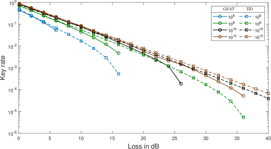
Figure 1: Key rate comparison for the qubit BB84 protocol with loss, between the GEAT analysis in this work (solid lines), and the IID setting (dashed lines). In all cases, the signals are depolarized with $p^{\mathrm{depol}}_{\mathrm{hon}}=0.01$, the security parameter is $\varepsilon^{\mathrm{secure}}=10^{-8}$, and for simplicity we show only the results for unique acceptance (see Remark 1). The testing probability $\gamma$ and the Rényi parameter $\alpha$ are optimized for the EAT analysis, and the former was also optimized in the IID analysis.

Next, in Fig. 2, we show a comparison between unique acceptance and a realistic acceptance set. The latter was chosen such that it fulfills the completeness condition $\Pr[\operatorname{freq}(c^{n})\notin S_{\mathrm{acc}}]\leq\varepsilon^{\mathrm{com}}$, where we chose $\varepsilon^{\mathrm{com}}=10^{-3}$, as laid out in Sec. 4.2 and Sec. 5.2.2. One can see that to achieve positive key rates up to $30\,\mathrm{dB}$, we require at least $n=10^{11}$ signals sent. However, there is only a small difference in the key rates between the unique-acceptance case and the realistic acceptance set. In practical protocols, one would need to use the latter option, since otherwise the protocol would just almost always abort. Hence, the fact that we incur such a small penalty when making the protocol robust against statistical fluctuations is an important feature for real-world implementations.

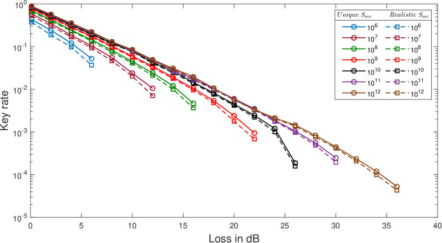
Figure 2: Key rates for the qubit BB84 protocol with loss. Solid lines correspond to the unique-acceptance condition (see Remark 1), whereas the dashed lines are for when there is a tolerance interval around the expected distribution as noted in Eq. (25). In all cases, signals are depolarized with $p^{\mathrm{depol}}_{\mathrm{hon}}=0.01$; the security parameter is $\varepsilon^{\mathrm{secure}}=10^{-8}$; the completeness parameter for the realistic tolerance intervals is $\varepsilon^{\mathrm{com}}=10^{-3}$; and the testing probability $\gamma$ and Rényi parameter $\alpha$ are optimized for each data point.

7 Decoy-state with improved analysis

In this section we will use our methods presented in Sec. 5, extend them to decoy-state protocols, and then apply the results to a decoy-state version of the BB84 protocol.

7.1 Protocol details

We present a decoy-state version of the BB84 protocol which is effectively a decoy-state version of our qubit example in Sec. 6 above. For this decoy-state protocol, Alice can choose between fully phase-randomized weak coherent pulses (WCP) with intensities $\{\mu_{\mathrm{sig}},\mu_{2},\mu_{3}\}$ to send her signals. The intensity $\mu_{\mathrm{sig}}$ is the so-called signal intensity and will be used predominantly for key generation. Furthermore, we assume that the information is encoded in the polarization degree of freedom, i.e. Alice will send states from the set $\{\rho_{H},\rho_{V},\rho_{D},\rho_{A}\}$, which are mixed because fully phase-randomized states are a classical mixture of photon-number states.

There are a few additional differences to the qubit BB84 protocol presented above. In each round Alice still decides with probability $\gamma$ whether it is a test or generation round. If it is a test round, Alice now selects an intensity $\mu_{i}\in\{\mu_{\mathrm{sig}},\mu_{2},\mu_{3}\}$ with some specified probability $p(\mu_{i}|t)$, and sends a uniformly random choice out of $\rho_{D},\rho_{A}$ in the $X$-basis with that intensity. Otherwise, she uses the signal intensity $\mu_{\mathrm{sig}}$ to send a uniformly random choice out of the states $\rho_{H},\rho_{V}$ in the $Z$-basis. In either case, she uses a classical register $X$ to record her choice of intensity, basis, and signal state.

We consider an active measurement setup where Bob has control over a polarization-rotator, which then determines the basis to be measured in. This choice is just out of convenience for our optimization problem, to keep the dimensions of the involved Choi states small. There are no inherent issues with using a passive detection setup, unlike methods relying on the entropic uncertainty relation, e.g. [LCW+14].

In case of a passive detection setup, one would be required to use alternative squashing maps unless $\gamma=1/2$, since the squashing map presented in [BML08, GBN+14] is only valid for passive setups with symmetric basis choices. For example, one could use the flag-state squasher of [ZCW+21] which allows for asymmetric basis choices of any detection setup, but requires a subspace estimation. A generic method for this subspace estimation for passive linear optical detection setups was presented in [KL24]. Hence, using the flag-state squasher would result in one additional constraint in (93) corresponding to the subspace estimation. Furthermore, Bob’s POVM elements would change due to his passive detection setup and by adding so-called flags necessary for the flag-state squasher. In summary, we stress that this procedure would allow us to incorporate any passive linear optical detection setup, but for this work we focus on an active detection setup to keep the dimension of our optimization variables small.

Applying the active detection setup, Bob still measures the incoming states with probability $\gamma$ in the $X$-basis and with $1-\gamma$ in the $Z$-basis, recording his basis choice and outcome. Bob then applies the post-processing of [BML08, GBN+14] for active BB84 detection setups to his outcomes. This converts his outcomes to an equivalent qubit detection scheme. Finally, Bob stores his post-processed outcomes in a classical register $Y$.

Then, the public announcements are also analogous to the previous qubit BB84 protocol. Alice first announces a classical register $C^{A}$ that is set to $\perp$ if it was a generation round, and otherwise set to the value of the $X$ register. Bob then announces a classical register $C^{B}$ as before: if it was a generation round (i.e. $C^{A}=\perp$) and he measured in the $Z$ basis, then he sets $C^{B}$ to either $(\mathtt{Z},\text{{det}})$ or $(\mathtt{Z},\text{{no-det}})$ depending on whether there was a detection; otherwise he sets $C^{B}=Y$. Just as in the qubit BB84 protocol, these form all the single-round public announcements, i.e. we have $I=(C^{A},C^{B})$; similarly, with these announcements Alice and Bob set $C=\perp$ if $C^{A}=\perp$, and otherwise set $C=(C^{A},C^{B})$. Then, they apply an analogous sifting procedure: if the round was a generation round that was also measured in the $Z$ basis and successfully detected (i.e. $C^{A}=\perp$ and $C^{B}=(\mathtt{Z},\mathtt{det})$), then Alice sets $S$ to be $0$ or $1$ depending on which $Z$-eigenstate she sent; otherwise she fixes $S=0$.

With this, the overall probability of a round passing the sifting stage is again $\left(1-\gamma\right)^{2}{p^{\mathtt{det}|\mathtt{ZZ}}_{\mathrm{hon}}}$. The value of $H(S|YI)_{\mathrm{hon}}$ in the error-correction term can hence be computed using the formula (73) as before, although the value of ${p^{\mathtt{det}|\mathtt{ZZ}}_{\mathrm{hon}}}$ is computed using the beamsplitter model for loss, but amounts to the same result ${p^{\mathtt{det}|\mathtt{ZZ}}_{\mathrm{hon}}}=1-p^{\mathrm{loss}}_{\mathrm{hon}}$.

7.2 General decoy formulation

We now lay out the the theoretical foundations for bounding the entropy against Eve. For flexibility in potential applications, in this description we will consider a slightly more general scenario than that described in Sec. 7.1 above. Specifically, we shall allow Alice to choose from multiple intensities $\mu_{\mathrm{sig}},\mu_{2},\dots$ in the generation rounds as well as the test rounds, according to some arbitrary distribution that may be different in the two cases. The protocol we described above can be viewed as the special case where the distribution in the generation rounds is the trivial distribution that always uses a single intensity $\mu_{\mathrm{sig}}$.

When using decoy states from WCP sources, we can assume without loss of generality that Eve performs a QND measurement of the photon number first and then applies an attack based on the photon number [LL20]. Thus, we can write Eve’s attack channel $\mathcal{E}$ as a direct sum acting on each photon number separately, $\mathcal{E}=\bigoplus_{n=0}^{\infty}\mathcal{E}_{n}$. The same holds true for the Choi states of the channel, i.e. $J=\bigoplus_{n=0}^{\infty}J_{n}$. Therefore, the states $\rho^{\mathrm{g}}_{J}$ conditioned on a generation round and $\rho^{t,\mu}_{J}$ conditioned on a test round with intensity $\mu$ satisfy

$$\rho^{\mathrm{g}}_{J}=\sum_{n}p(n)\rho_{J_{n}}^{g},\qquad\rho^{\mathrm{t,\mu}}_{J}=\sum_{n}p_{\mu}(n)\rho^{\mathrm{t,\mu}}_{J_{n}}.$$ (85)

For any protocol we can find a lower bound on the objective in the crossover rate function (40) by ignoring all contributions apart from those of single photons sent by Alice. In the case of the BB84 protocol this will be the main contribution, whereas vacuum states would only contribute on the order of dark counts. All higher photon numbers will not contribute to increasing the key rate because Eve could perform a PNS attack [BBB+92, BLM+00]. Nevertheless, our technique allows for including higher photon numbers in principle, which could be beneficial for other protocols.

As the single-photon contribution to the objective function only depends on the Choi state $J_{1}$, from the above consideration we see the crossover rate function can be lower bounded via

$$\begin{aligned} r_{\mathrm{cross}}(\mathbf{q})\geq\inf_{J=\bigoplus_{n=1}^{\infty}J_{n}}&\quad p(1)W(\rho_{J_{1}}^{g})\\ \text{ s.t.}&\quad\mathbf{\Phi}[\rho^{\mathrm{t}}_{J}]=\mathbf{q},\end{aligned}$$ (86)

whereas if we were to consider additional photon numbers up to some cut-off $N_{c}$, we would replace $p(1)W(\rho_{J_{1}}^{g})$ with

$$\sum_{n\leq N_{c}}p(n)W(\rho_{J_{n}}^{g}),$$ (87)

and the optimization variables appearing in the objective function would include all Choi states up to $N_{c}$.

Similarly to the objective function, one can exploit the block-diagonal structure of the Choi states for $\mathbf{\Phi}[\rho^{\mathrm{t,\mu}}_{J}]$. Here we can equivalently write for each intensity $\mu$

$$\mathbf{\Phi}[\rho^{\mathrm{t,\mu}}_{J}]=\sum_{n=0}^{\infty}p_{\mu}(n)\mathbf{\Phi}[\rho^{\mathrm{t,\mu}}_{J_{n}}].$$ (88)

For simplicity let us write $\mathbf{q}^{\mu}$ to denote the component of $\mathbf{q}$ corresponding to the intensity $\mu$, i.e. so we have $\mathbf{q}=\left(\mathbf{q}^{\mu_{\mathrm{sig}}},\mathbf{q}^{\mu_{2}},\dots\right)$ and $\sum_{c}\mathbf{q}^{\mu}_{c}=p(\mu|t)$.

Next, for each $c=(a,b)\in\mathcal{C}_{\setminus\perp}$ we can make the following rearrangements by writing $\mathbf{\Phi}[\rho^{\mathrm{t,\mu}}_{J_{n}}]_{ab}=p(a,b|\mu,n)=:Y_{n}^{ab}$:

$$\mathbf{q}^{\mu}=p(\mu|t)\mathbf{\Phi}_{ab}[\rho^{\mathrm{t,\mu}}_{J}]=p(\mu|t)\sum_{n=0}^{\infty}p_{\mu}(n)\mathbf{\Phi}_{ab}[\rho^{\mathrm{t,\mu}}_{J_{n}}]=p(\mu|t)\sum_{n=0}^{\infty}p_{\mu}(n)Y_{n}^{ab},$$ (89)

where we chose the definition of the $n$-photon yield $Y_{n}^{ab}$ in line with the common one used for decoy-state protocols. These yields actually do not depend on the intensity $\mu$, because based on the photon number Eve is unable to distinguish the intensities [LL20].

With this formulation, observe that for all $n\neq 1$, the only dependence of our optimization on the Choi states $J_{n}$ is via the corresponding yields $\mathbf{Y}_{n}$. Therefore, we can optimize over the yields $\mathbf{Y}_{n}$ in place of those Choi states. However, since this would still contain an infinite number of optimization variables, we introduce a photon number cut-off $N_{\mathrm{ph}}$ and characterize the remainder of the sum by $\boldsymbol{\delta}^{\mu}$. The remainder $\boldsymbol{\delta}^{\mu}$ cannot be arbitrarily large; it needs to satisfy for each intensity $\mu$:

$$0\leq\delta_{ab}^{\mu}\leq 1-\sum_{n\leq N_{\mathrm{ph}}}p_{\mu}(n)=:1-p_{\mathrm{tot}}(\mu)\quad\forall(a,b)\in\mathcal{C}.$$ (90)

Therefore, for some $\delta_{ab}^{\mu}$ satisfying the above constraint, we can write

$$\mathbf{\Phi}_{ab}[\rho^{\mathrm{t,\mu}}_{J}]=\sum_{n=0}^{N_{\mathrm{ph}}}p_{\mu}(n)Y_{n}^{ab}+\delta_{ab}^{\mu},$$ (91)

for all intensities $\mu$. Hence, we can recast the final optimization problem for the crossover rate function as

$$\begin{aligned} r_{\mathrm{cross}}(\mathbf{q})\geq\inf_{J_{1},\mathbf{Y}_{0},\dots\mathbf{Y}_{N_{\mathrm{ph}}},\boldsymbol{\delta}^{\mu}}&\quad p(1)W(\rho_{J_{1}}^{g})\\ \text{ s.t.}&\quad p(\mu|t)\left(\sum_{n\leq N_{\mathrm{ph}}}p_{\mu}(n)\mathbf{Y}_{n}+\boldsymbol{\delta}^{\mu}\right)=\mathbf{q}^{\mu}\;\forall\mu,\\ &\quad 0\leq\boldsymbol{\delta}^{\mu}\leq 1-p_{\mathrm{tot}}(\mu)\;\forall\mu,\\ &\quad p(\mu|t)\mathbf{Y}_{1}=p(\mu|t)\mathbf{\Phi}[\rho^{\mathrm{t,\mu}}_{J_{1}}]\;\forall\mu,\\ &\quad\sum_{b}Y^{ab}_{n}=p(a|t,n)\;\forall a,b.\end{aligned}$$ (92)

Before we continue to the decoy version of the optimization problem in Theorem 4, a few remarks about this crossover rate function are in line. As mentioned earlier, the crossover rate function yields the secret key rate for collective attacks, and hence can be used to compute valid key rates in the asymptotic limit as well. Thus, one can draw simple comparisons to previous decoy-state methods.

For example, in [WL22], asymptotic key rates were calculated for decoy-state protocols. In that work a two-step process was performed, where first the single-photon yields $\mathbf{Y}_{1}$ were bounded from above and below using an LP, and then these bounds were used to calculate the secret key rate. Additionally, in [NUL23, KL24] improved methods for the decoy-state analysis were developed. Those works already used the Choi state to characterize the channel, but only for the purposes of bounding the single-photon yields, i.e. the overall key rate calculation was still a two-step process.

Our methods here combine these two steps into a single one, which should provide strictly better results. This is due to the fact that imposing bounds on $\mathbf{Y}_{1}=\mathbf{\Phi}[\rho^{\mathrm{t,\mu}}_{J_{1}}]$ only, which is what is done in the two-step process of the previously mentioned works, will only result in a lower optimal value. Hence, even on the level of the asymptotic key rates, the formulation of Eq. (92) will result in higher secret key rates.

Next we turn our attention to finding an optimal crossover min-tradeoff function as in Theorem 4. We still define $r_{\mathrm{best}}$ in the same way, but instead we use the modified crossover rate function of Eq. (92) from above. After following the same steps as in Appendix A, we find

$$\begin{aligned} r_{\mathrm{best}}=\inf_{\begin{subarray}{c}J_{1},\mathbf{Y}_{0},\dots\mathbf{Y}_{N_{\mathrm{ph}}},\\ \boldsymbol{\delta}^{\mu},\boldsymbol{\tau}^{\mu}\end{subarray}}&\quad p(1)W(\rho_{J_{1}}^{g})+s\!\left(\sum_{c}\tau_{c}/{2}\right)\\ \text{ s.t.}&\quad-\boldsymbol{\tau}^{\mu}\leq\mathbf{q}^{\mu}-p(\mu|t)\left(\sum_{n\leq N_{\mathrm{ph}}}p_{\mu}(n)\mathbf{Y}_{n}+\boldsymbol{\delta}^{\mu}\right)\leq\boldsymbol{\tau}^{\mu}\;\forall\mu,\\ &\quad 0\leq\boldsymbol{\delta}^{\mu}\leq 1-p_{\mathrm{tot}}(\mu)\;\forall\mu,\\ &\quad p(\mu|t)\mathbf{Y}_{1}=p(\mu|t)\mathbf{\Phi}[\rho^{\mathrm{t,\mu}}_{J_{1}}]\;\forall\mu,\\ &\quad\sum_{b}Y^{ab}_{n}=p(a|t,n)\;\forall a,b.\end{aligned}$$ (93)

As before, the gradient of the crossover min-tradeoff function can be extracted as the dual variable to the constraint $\mathbf{q}^{\mathrm{hon}}-\mathbf{\Phi}[\rho^{\mathrm{t}}_{J}]-\boldsymbol{\lambda}=\mathbf{0}$, where $\mathbf{q}^{\mathrm{hon}}=\left(\mathbf{q}^{\mu_{\mathrm{sig}}},\dots\right)^{T}$, $\mathbf{\Phi}[\rho^{\mathrm{t}}_{J}]=\left(p(\mu|t)\mathbf{\Phi}[\rho^{\mathrm{t,\mu}}_{J}],\dots\right)^{T}$ and each $\mathbf{\Phi}[\rho^{\mathrm{t,\mu}}_{J}]$ is identified by Eq. (91). This constraint is, as expected, equivalent to the first constraint of our optimization problem for $r_{\mathrm{best}}$:

$$\mathbf{0}=\mathbf{q}^{\mu}-p(\mu|t)\left(\sum_{n\leq N_{\mathrm{ph}}}p_{\mu}(n)\mathbf{Y}_{n}+\boldsymbol{\delta}^{\mu}\right)-\boldsymbol{\lambda}^{\mu}\quad\forall\mu.$$ (94)

After we find the gradient $\mathbf{g}$ of a crossover min-tradeoff function, we can again apply the key length formula from Eq. (16):

$$l \leq n\left(\inf_{\begin{subarray}{c}J_{1},\mathbf{Y}_{0},\dots\mathbf{Y}_{N_{\mathrm{ph}}},\\ \mathbf{\delta}^{\mu}\end{subarray}}\left(p(1)W(\rho_{J_{1}}^{g})+\mathbf{g}\cdot\left(\mathbf{q}^{\mathrm{hon}}-\mathbf{\Phi}[\rho^{\mathrm{t}}_{J}]\right)-\frac{\alpha-1}{2-\alpha}\frac{\operatorname{ln}(2)}{2}\widetilde{V}\!\left(\mathbf{\Phi}[\rho^{\mathrm{t}}_{J}],\mathbf{g}\right)\right)-\Delta_{\mathrm{com}}\right)$$

$$\qquad-n\left(\frac{\alpha-1}{2-\alpha}\right)^{2}K(\alpha)-\lambda_{\mathrm{EC}}-\frac{\alpha}{\alpha-1}\log\frac{1}{\varepsilon^{\mathrm{secret}}}+2,$$ (95)

where now $\mathbf{q}^{\mathrm{hon}}=\left(\mathbf{q}^{\mu_{\mathrm{sig}}},\dots\right)^{T}$, $\mathbf{\Phi}[\rho^{\mathrm{t}}_{J}]=\left(p(\mu|t)\mathbf{\Phi}[\rho^{\mathrm{t,\mu}}_{J}],\dots\right)^{T}$ and

$$p(\mu|t)\mathbf{\Phi}[\rho^{\mathrm{t,\mu}}_{J}]=p(\mu|t)\left(\sum_{n\leq N_{\mathrm{ph}}}p_{\mu}(n)\mathbf{Y}_{n}+\boldsymbol{\delta}^{\mu}\right)$$ (96)

is a function of $\mathbf{Y}_{0},\dots,\mathbf{Y}_{N_{\mathrm{ph}}},\boldsymbol{\delta}^{\mu}$. Thus, we have found a formulation in line with Sec. 5 and can apply those methods to calculate the finite-size secret key rates. Again, if we were to include higher photon numbers, the term $p(1)W(\rho_{J_{1}}^{g})$ will be replaced with $\sum_{n}p(n)W(\rho_{J_{n}}^{g})$.

7.3 Numerical results

In this section we present our numerical results for the decoy-state BB84 protocol as described in Sec. 7.1. Again, note that we only consider the single-photon contribution (any higher photon number will give zero key rate) as shown in the derivation of (93). Hence, $W(\rho_{J_{1}}^{g})$ is equal to $W(\rho^{\mathrm{g}}_{J})$ in Eq. (74) of the qubit BB84 protocol. Therefore, also the Kraus operators for the $\mathcal{G}$-map of eq. (77) and the $\mathcal{Z}$-map of eq. (78) apply for the decoy-state protocol as well.

In Fig. 3 we show the secret key rates for the decoy-state BB84 protocol, plotted against loss in $\mathrm{dB}$. We suppose that the honest implementation is subject to misalignment with an angle of $\theta_{\text{misalign}}=\sin^{-1}(0.1)\approx 0.1002$ under the model described in [WL22]. We chose the intensities as $\{\mu_{\mathrm{sig}}=0.9,\mu_{2}=2\times 10^{-2},\mu_{3}=10^{-3}\}$, the photon number cut-off as $N_{\mathrm{ph}}=10$, and the security parameter as $\varepsilon^{\mathrm{secure}}=10^{-8}$. For each data point we optimized the testing probability $\gamma$ and the Rényi parameter.

As in the case of the qubit BB84 protocol, the key rates resulting from our proof technique are mostly lower than the IID key rates from [KTL24] for the same protocol. Again, since we prove security against a wider class of attacks, one could expect such a behaviour. We see that to reach positive key rates for losses up to $25\,\mathrm{dB}$, we require about $10^{12}$ signals sent.

We point out however that in the low-loss regime, we can approximately reach the asymptotic value with $n=10^{12}$ signals, and for those data points it can be seen from the figure that we actually have a slight improvement over the IID analysis from [KTL24] (which was based on previous decoy methods). Thus, we confirm that our improved method can indeed improve the key rates as compared to previous methods, albeit only slightly.

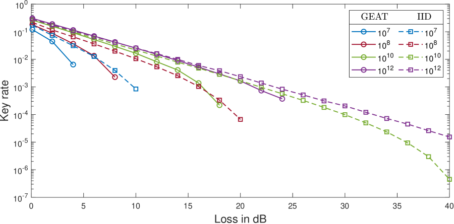
Figure 3: Key rate comparison for the decoy-state protocol, between the GEAT analysis in this work (solid lines), and the IID setting (dashed lines). In all cases, fully phase-randomized weak coherent pulses with intensities $\{\mu_{\mathrm{sig}}=0.9,\mu_{2}=10^{-2},\mu_{3}=10^{-3}\}$ were used. Signals are misaligned with $\theta_{\text{misalign}}=0.1002$, the photon number cut-off is $N_{\mathrm{ph}}=10$, the security parameter is $\varepsilon^{\mathrm{secure}}=10^{-8}$, and for simplicity we show only the results for unique acceptance (see Remark 1). The testing probability $\gamma$ and the Rényi parameter $\alpha$ are optimized for the EAT analysis, and the former was also optimized for the IID analysis.

Finally, in Fig. 4, we also present a comparison between unique acceptance and realistic acceptance sets for the decoy-state BB84 protocol. We note that in this case, the influence of a realistic acceptance set is much more pronounced than for the ideal qubit protocol. In particular, as the channel loss increases and the protocol approaches its maximum tolerable loss, the penalty from realistic acceptance sets becomes more significant. This could potentially be improved by applying adaptive key rate formulations such as in [TTL24, HB24].

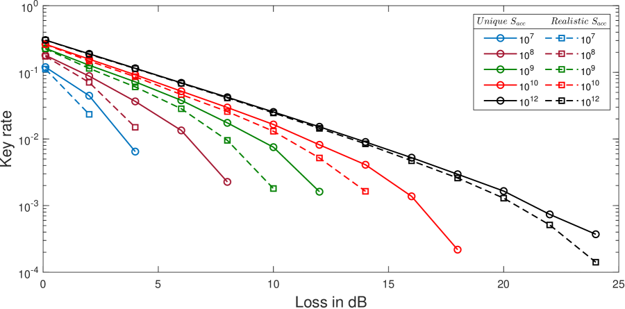
Figure 4: Key rates for the decoy-state protocol. Solid lines correspond to the unique-acceptance condition (see Remark 1), whereas the dashed lines are for when there is a tolerance interval around the expected distribution as noted in Eq. (25). In all cases, two decoy signals are used with intensities $\mu_{2}=3\times 10^{-2}$ and $\mu_{2}=10^{-3}$, while the actual signal has the intensity of $\mu_{\mathrm{sig}}=0.9$, and the signals are chosen uniformly at random in each round. Signals are misaligned with $\theta_{\text{misalign}}=0.1002$, the photon number cut-off is $N_{\mathrm{ph}}=10$, the security parameter is chosen to be $\varepsilon^{\mathrm{secure}}=10^{-8}$, and the completeness parameter for the realistic tolerance intervals is $\varepsilon^{\mathrm{com}}=10^{-3}$. The testing probability $\gamma$ and the Rényi parameter $\alpha$ are optimized for each data point. From the graph, it can be seen that similar to the qubit BB84 protocol with loss in Sec. 6, as the number of signals is increased the difference between the two cases decreases.

8 Conclusion

In summary, in this work we have developed a flexible framework for security proofs of PM protocols against general attacks, with a particular focus on decoy-state protocols. To do so, we introduced techniques for analyzing decoy-state protocols that are compatible with the GEAT, and have the further advantage that since they merge several steps that were handled separately in previous works [WL22, NUL23, KL24], they should yield improved key rates even in the IID case. Furthermore, we implemented a number of methods to improve the finite-size terms arising from the GEAT, including a method to optimize the choice of min-tradeoff function, and incorporating various improvements to the finite-size terms. By applying our framework to an example of a decoy-state protocol, we show that reasonably robust key rates can be achieved even in the finite-size regime.

We highlight that by using using the GEAT rather than the EAT in this work, we have also obtained an important advantage in that the resulting key rates have a reasonable level of loss tolerance, overcoming a difficulty noticed in the EAT-based analysis of [GLH+22]. More specifically, due to some technical issues regarding the EAT Markov conditions, the finite-size key rates computed from the EAT always had a subtractive penalty on the order of the test-round probability $\gamma$. This caused an issue that in any loss regime where the asymptotic key rate was of similar order of magnitude to $\gamma$, it was not possible to obtain positive finite-size key rates, due to this subtractive penalty. In contrast, for a GEAT-based security proof, the effect of the test-round announcements is essentially just to rescale the first-order term by a multiplicative penalty, which is much less significant.

Finally, we note that as mentioned in the introduction, we rely on recent work [HB24, AHT24] to argue that the keyrates computed in this work are also valid without restricting Eve to only interact with a single signal at a time. However, the results in those works also give sharper bounds on the final Rényi entropy produced in the protocol, which should yield better keyrates. We highlight that the techniques we developed here, especially for solving optimizations with a modified objective function as in Eq. (93), are also naturally compatible with the bounds derived in [AHT24]. Furthemore, while here we have focused on protocols producing a key of fixed length, the techniques in [HB24] yield a very natural security proof framework for protocols producing variable-length keys, and the techniques in [AHT24] can be incorporated into that analysis. Hence we aim to consolidate these approaches in future work. As a starting point, for readers already familiar with [AHT24], we discuss in Appendix B some further details relevant to analyzing optical QKD protocols with the proof techniques in that work; specifically, sharper conversions between Rényi entropy and von Neumann entropy.

Computational platform

The computations in this work were performed using the MATLAB package CVX [GB14] with the solver MOSEK [MOS19].

Appendix A Deriving modified optimization

In this appendix, we give the proof of Theorem 4. We begin by proving the following lemma:

Lemma 1.

For any constants $\varphi_{0},\varphi_{1}\geq 0$, the function $\hat{T}$ defined in (58) is a convex function with Legendre-Fenchel conjugate $\hat{T}^{*}$ given by (60), and satisfies

$$\hat{T}(\mathbf{g})=\hat{T}^{**}(\mathbf{g})=\sup_{\boldsymbol{\lambda}}\left(\mathbf{g}\cdot\boldsymbol{\lambda}-\hat{T}^{*}(\boldsymbol{\lambda})\right).$$ (97)

Proof.

We start the proof by showing that $\hat{T}(\mathbf{g})$ is a convex function. We first restate the definition of $\hat{T}$ from (58):

$$\hat{T}(\mathbf{g})\coloneqq\varphi_{0}(\left(\max(\mathbf{g})-\min(\mathbf{g})\right)^{2}+\varphi_{1}\left(\max(\mathbf{g})-\min(\mathbf{g})\right).$$

First note that $\max(\mathbf{g})$ is convex and $\min(\mathbf{g})$ is concave. Thus, $\max(\mathbf{g})-\min(\mathbf{g})$ is convex; moreover, it is non-negative, therefore, its square is also a convex function. By noting that $\varphi_{0},\varphi_{1}\geq 0$, we conclude $\hat{T}(\mathbf{g})$ is a convex function.

Now to prove its Legendre-Fenchel conjugate is the expression (60), we first write out the definition of the conjugate (see e.g. [BV04] Chapter 3.3):

$$\hat{T}^{*}(\boldsymbol{\lambda})=\sup_{\mathbf{g}}\left(\mathbf{g}\cdot\boldsymbol{\lambda}-\varphi_{0}(\left(\max(\mathbf{g})-\min(\mathbf{g})\right)^{2}-\varphi_{1}\left(\max(\mathbf{g})-\min(\mathbf{g})\right)\right).$$ (98)

Let us first consider the case where the sum of the elements of $\boldsymbol{\lambda}$ is zero, i.e., $\sum_{c}\lambda_{c}=0$. Note that for any vector $\mathbf{g}$, we can define another vector $\tilde{\mathbf{g}}$, whose elements are given by:

$$\tilde{g}_{c}=\begin{cases}\max(g)&\text{ if }\lambda_{c}\geq 0\\ \min(g)&\text{ otherwise }\end{cases}.$$ (99)

It is not hard to see that for any vector $\mathbf{g}$, the quantity within the supremum in (98) is upper bounded by the value with $\tilde{\mathbf{g}}$ in place of $\mathbf{g}$. Furthermore, letting $\mathcal{C}_{\geq 0}$ be the set of $c$ values with $\lambda_{c}\geq 0$, we have

$$\tilde{\mathbf{g}}\cdot\boldsymbol{\lambda}=\max(g)\sum_{c\in\mathcal{C}_{\geq 0}}\lambda_{c}+\min(g)\sum_{c\notin\mathcal{C}_{\geq 0}}\lambda_{c}=(\max(g)-\min(g)){\left\lVert\boldsymbol{\lambda}\right\rVert_{1}}/{2},$$ (100)

using the fact that $\sum_{c\in\mathcal{C}_{\geq 0}}\lambda_{c}=-\sum_{c\notin\mathcal{C}_{\geq 0}}\lambda_{c}={\left\lVert\boldsymbol{\lambda}\right\rVert_{1}}/{2}$ since $\sum_{c}\lambda_{c}=0$. Therefore, the RHS of (98) simplifies to

$$\hat{T}^{*}(\boldsymbol{\lambda}) =\sup_{\mathbf{g}}\left(({\left\lVert\boldsymbol{\lambda}\right\rVert_{1}}/{2}-\varphi_{1})\left(\max(\mathbf{g})-\min(\mathbf{g})\right)-\varphi_{0}\left(\max(\mathbf{g})-\min(\mathbf{g})\right)^{2}\right)$$ (101)

$$=\sup_{\beta\geq 0}\left(({\left\lVert\boldsymbol{\lambda}\right\rVert_{1}}/{2}-\varphi_{1})\beta-\varphi_{0}\beta^{2}\right),$$ (102)

where in the second line, we use the fact that the optimization only depends on the difference $\max(\mathbf{g})-\min(\mathbf{g})$. The optimization in (101) can be solved using simple calculus which leads to the following:

$$\hat{T}^{*}(\boldsymbol{\lambda})=\begin{cases}\frac{({\left\lVert\boldsymbol{\lambda}\right\rVert_{1}}/{2}-\varphi_{1})^{2}}{4\varphi_{0}}&\text{if}\left\lVert\boldsymbol{\lambda}\right\rVert_{1}\geq 2\varphi_{1}\\ 0&\text{if}\left\lVert\boldsymbol{\lambda}\right\rVert_{1}<2\varphi_{1}\end{cases}$$ (103)

Let us now look at the situation where $\sum_{c}\lambda_{c}\neq 0$. Consider the particular choice $\mathbf{g}=k\mathbf{1}$ for some $k\in\mathbb{R}$. Taking the supremum over such choices of $\mathbf{g}$, from (98) we have:

$$\hat{T}^{*}(\boldsymbol{\lambda}) \geq\sup_{k}\left(k\sum_{c}\lambda_{c}\right)$$ (104)

$$=+\infty,$$ (105)

where the second equality follows by setting $k\rightarrow+\infty$ (resp. $k\rightarrow-\infty$) if $\sum_{c}\lambda_{c}>0$ (resp. $\sum_{c}\lambda_{c}<0$). Combining (103) with (104) results the expression in (60).

Finally, to show that (97) holds, we simply use the fact that $\hat{T}$ is a convex function with its domain being all of $\mathbb{R}^{|\mathcal{C}|-1}$. Therefore its epigraph is a convex closed set, and hence it is equal to the conjugate of its conjugate (see e.g. [BV04] Chapter 3.3.2), i.e. we have $\hat{T}(\mathbf{g})=\hat{T}^{**}(\mathbf{g})=\sup_{\boldsymbol{\lambda}}\left(\mathbf{g}\cdot\boldsymbol{\lambda}-\hat{T}^{*}(\boldsymbol{\lambda})\right)$ as claimed. ∎

With this, we turn to proving the first equality (62) in Theorem 4. First, recall that as discussed in Sec. 4.3, any $\mathbf{g}$ and $k_{g}$ satisfying the condition $\mathbf{g}\cdot\mathbf{q}+k_{g}\leq r_{\mathrm{cross}}(\mathbf{q})$ (for all $\mathbf{q}$) yields a valid crossover min-tradeoff function. This means that in fact any gradient vector $\mathbf{g}$ corresponds to some valid choice(s) of crossover min-tradeoff function, simply by choosing $k_{g}$ to be some value satisfying that condition (such values always exist because $r_{\mathrm{cross}}(\mathbf{q})$ is a non-negative convex function). Now observe that in the supremum over crossover min-tradeoff functions in (61), for any fixed $\mathbf{g}$, the best choice of $k_{g}$ would be the highest possible value satisfying that condition. Specifically, this implies we should choose it to be as follows, recalling that by definition an infimum is the highest possible lower bound on a set (see [TSB+22] Sec. 5 for another perspective based on Lagrange duals):

$$k_{g} =\inf_{\mathbf{q}}\left(r_{\mathrm{cross}}(\mathbf{q})-\mathbf{g}\cdot\mathbf{q}\right)$$

$$=\inf_{J}\left(W(\rho^{\mathrm{g}}_{J})-\mathbf{g}\cdot\mathbf{\Phi}[\rho^{\mathrm{t}}_{J}]\right),$$ (106)

where in the second line we have substituted in the definition of $r_{\mathrm{cross}}(\mathbf{q})$ from (40), with $\rho^{\mathrm{g}}_{J},\rho^{\mathrm{t}}_{J}$ being again understood as functions of $J$ via (38). Hence, we should always take the scalar term $k_{g}$ in the optimization (61) to be given by the above expression.

Substituting the formulas (97) and (106) into the argument of the supremum in (61), it becomes

$$\mathbf{g}\cdot\mathbf{q}^{\mathrm{hon}}+\inf_{J}\left(W(\rho^{\mathrm{g}}_{J})-\mathbf{g}\cdot\mathbf{\Phi}[\rho^{\mathrm{t}}_{J}]\right)-\sup_{\boldsymbol{\lambda}}\left(\mathbf{g}\cdot\boldsymbol{\lambda}-\hat{T}^{*}(\boldsymbol{\lambda})\right)$$

$$=\, \inf_{(J,\boldsymbol{\lambda})\in\mathcal{D}}\left(W(\rho^{\mathrm{g}}_{J})+\hat{T}^{*}(\boldsymbol{\lambda})+\mathbf{g}\cdot\left(\mathbf{q}^{\mathrm{hon}}-\mathbf{\Phi}[\rho^{\mathrm{t}}_{J}]-\boldsymbol{\lambda}\right)\right),$$ (107)

where $\mathcal{D}$ is a convex set defined as the set of tuples $(J,\boldsymbol{\lambda})$ such that $J$ is a Choi matrix and $\boldsymbol{\lambda}\in\mathbb{R}^{|\mathcal{C}|-1}$ satisfies $\sum_{c}\lambda_{c}=0$ (we can restrict the optimization over $\boldsymbol{\lambda}$ to such values without loss of generality, because $\hat{T}(\mathbf{g})=+\infty$ whenever $\sum_{c}\lambda_{c}\neq 0$). Our goal is to find the choice of $\mathbf{g}$ that maximizes the above value, in other words to find the optimal solution $\mathbf{g}$ to

$$\sup_{\mathbf{g}}\inf_{(J,\boldsymbol{\lambda})\in\mathcal{D}}\left(W(\rho^{\mathrm{g}}_{J})+\hat{T}^{*}(\boldsymbol{\lambda})+\mathbf{g}\cdot\left(\mathbf{q}^{\mathrm{hon}}-\mathbf{\Phi}[\rho^{\mathrm{t}}_{J}]-\boldsymbol{\lambda}\right)\right).$$ (108)

(Note that in the above, the objective function is finite everywhere over the domain $\mathcal{D}$, so we do not have issues with domain definitions.) We now simply observe that the above problem is precisely the Lagrange dual of the constrained convex optimization

$$\begin{aligned} \inf_{(J,\boldsymbol{\lambda})\in\mathcal{D}}&\quad W(\rho^{\mathrm{g}}_{J})+\hat{T}^{*}(\boldsymbol{\lambda})\\ \text{ s.t.}&\quad\mathbf{q}^{\mathrm{hon}}-\mathbf{\Phi}[\rho^{\mathrm{t}}_{J}]-\boldsymbol{\lambda}=\mathbf{0},\end{aligned}$$ (109)

and furthermore this constrained optimization satisfies strict feasibility, for instance by setting $J=\mathbb{I}$ and $\boldsymbol{\lambda}=\mathbf{q}^{\mathrm{hon}}-\mathbf{\Phi}[\rho^{\mathrm{t}}_{\mathbb{I}}]$ (this point indeed lies in the relative interior of $\mathcal{D}$, because $J=\mathbb{I}$ is in the relative interior of the set of Choi matrices, and $\sum_{c}\lambda_{c}=0$ by (66)). Hence by Slater’s condition ([BV04] Chapter 5.2.3), we have strong duality, i.e. the optimizations (108) and (109) have the same optimal value, and the optimal dual solution $\mathbf{g}$ is attained. From (109), we obtain the desired equality (62) by simply noting that the $\sum_{c}\lambda_{c}=0$ restriction in the domain $\mathcal{D}$ is already enforced by the $\mathbf{q}^{\mathrm{hon}}-\mathbf{\Phi}[\rho^{\mathrm{t}}_{J}]-\boldsymbol{\lambda}=\mathbf{0}$ constraint (see (66)).

Turning to the next equality (63), it is a straightforward transformation of the optimization problem that can be derived as follows. First observe that the optimization in (62) is clearly lower bounded by the optimization in (63) because every feasible point $(J,\boldsymbol{\lambda})$ in the former yields a feasible point $(J^{\prime},\boldsymbol{\lambda}^{\prime},\boldsymbol{\tau}^{\prime})$ of the latter with the same objective value, simply by taking $J^{\prime}=J$, $\boldsymbol{\lambda}^{\prime}=\boldsymbol{\lambda}$ and $\tau^{\prime}_{c}=|\lambda_{c}|$. Conversely, the optimization in (63) is also lower bounded by the optimization in (62), because every feasible point $(J,\boldsymbol{\lambda},\boldsymbol{\tau})$ in the former yields a feasible point $(J^{\prime},\boldsymbol{\lambda}^{\prime})$ of the latter with an objective value that is no higher, by taking $J^{\prime}=J$ and $\boldsymbol{\lambda}^{\prime}=\boldsymbol{\lambda}$ (in which case we have $\sum_{c}\tau_{c}\geq\left\lVert\boldsymbol{\lambda}^{\prime}\right\rVert_{1}$ and hence $s\!\left(\sum_{c}\tau_{c}/{2}\right)\geq s\!\left(\left\lVert\boldsymbol{\lambda}^{\prime}\right\rVert_{1}/2\right)=\hat{T}^{*}(\boldsymbol{\lambda}^{\prime})$, since $s$ is a monotone increasing function and $\sum_{c}\lambda^{\prime}_{c}=0$ by (66)). Hence, the optimizations in (62) and (63) are equal.

Finally, we turn to proving the last bound (65). The intuition behind this property is that as mentioned above, the optimal dual solution to (109) is in fact the optimal choice of $\mathbf{g}$ in (61). However, since in arriving at the SDP (64) we have implemented several transformations of the domain, objective and constraints in the “fundamental” optimization (109), it is not immediately clear whether this property is inherited by the dual of the SDP (64). Hence, we shall instead directly prove the bound (65) via an appropriate series of inequalities.

First note that the SDP (64) is again strictly feasible (e.g. following the above ideas, by choosing $J=\mathbb{I}$, $\boldsymbol{\lambda}=\mathbf{q}^{\mathrm{hon}}-\mathbf{\Phi}[\rho^{\mathrm{t}}_{\mathbb{I}}]$ and any $\tau_{c}>|\lambda_{c}|$) and hence by Slater’s condition, the dual is attained and has the same optimal value $r_{\mathrm{SDP}}$. By the definition of Lagrange duality, this means the optimal dual solution to the $\mathbf{q}^{\mathrm{hon}}-\mathbf{\Phi}[\rho^{\mathrm{t}}_{J}]-\boldsymbol{\lambda}=\mathbf{0}$ constraint in the SDP (64) is a vector $\mathbf{g}^{\star}\in\mathbb{R}^{\left|\mathcal{C}_{\setminus\perp}\right|}$ such that

$$\begin{aligned} r_{\mathrm{SDP}}=\;\inf_{(J,\boldsymbol{\lambda},\boldsymbol{\tau})\in\mathcal{D}^{\prime}}&\quad L(\rho^{\mathrm{g}}_{J},\boldsymbol{\tau})+\mathbf{g}^{\star}\cdot\left(\mathbf{q}^{\mathrm{hon}}-\mathbf{\Phi}[\rho^{\mathrm{t}}_{J}]-\boldsymbol{\lambda}\right),\end{aligned}$$ (110)

where for compactness we introduce the following notation: $\mathcal{D}^{\prime}$ denotes the set of tuples $(J,\boldsymbol{\lambda},\boldsymbol{\tau})$ such that $J$ is a Choi matrix and $\boldsymbol{\lambda},\boldsymbol{\tau}\in\mathbb{R}^{|\mathcal{C}|-1}$ are vectors satisfying $-\boldsymbol{\tau}\leq\boldsymbol{\lambda}\leq\boldsymbol{\tau}$ (i.e. it incorporates the constraints other than $\mathbf{q}^{\mathrm{hon}}-\mathbf{\Phi}[\rho^{\mathrm{t}}_{J}]-\boldsymbol{\lambda}=\mathbf{0}$ in the SDP (64)).

With this, note that given the above choice of gradient $\mathbf{g}^{\star}$, if we choose the scalar term in $g^{\star}$ according to (106) then the desired result (65) holds:

$$g^{\star}(\mathbf{q}^{\mathrm{hon}})-\hat{T}(\mathbf{g}^{\star}) =\mathbf{g}^{\star}\cdot\mathbf{q}^{\mathrm{hon}}+\inf_{J}\left(W(\rho^{\mathrm{g}}_{J})-\mathbf{g}^{\star}\cdot\mathbf{\Phi}[\rho^{\mathrm{t}}_{J}]\right)-\sup_{\boldsymbol{\lambda}}\left(\mathbf{g}^{\star}\cdot\boldsymbol{\lambda}-\hat{T}^{*}(\boldsymbol{\lambda})\right)$$

$$=\inf_{(J,\boldsymbol{\lambda})\in\mathcal{D}}\left(W(\rho^{\mathrm{g}}_{J})+\hat{T}^{*}(\boldsymbol{\lambda})+\mathbf{g}^{\star}\cdot\left(\mathbf{q}^{\mathrm{hon}}-\mathbf{\Phi}[\rho^{\mathrm{t}}_{J}]-\boldsymbol{\lambda}\right)\right)$$

$$=\inf_{(J,\boldsymbol{\lambda},\boldsymbol{\tau})\in\mathcal{D}^{\prime}}\left(W(\rho^{\mathrm{g}}_{J})+s\!\left(\sum_{c}\tau_{c}/{2}\right)+\mathbf{g}^{\star}\cdot\left(\mathbf{q}^{\mathrm{hon}}-\mathbf{\Phi}[\rho^{\mathrm{t}}_{J}]-\boldsymbol{\lambda}\right)\right)$$

$$\geq\inf_{(J,\boldsymbol{\lambda},\boldsymbol{\tau})\in\mathcal{D}^{\prime}}\left(L(\rho^{\mathrm{g}}_{J},\boldsymbol{\tau})+\mathbf{g}^{\star}\cdot\left(\mathbf{q}^{\mathrm{hon}}-\mathbf{\Phi}[\rho^{\mathrm{t}}_{J}]-\boldsymbol{\lambda}\right)\right)$$

$$=r_{\mathrm{SDP}},$$ (111)

where each line is justified as follows. The first and second lines are obtained by simply substituting (97) and (106) and then simplifying the resulting expression, similar to before. The third line holds by the same arguments as in the above derivation of (63). The fourth line holds because $L(\rho^{\mathrm{g}}_{J},\boldsymbol{\tau})$ is a lower bound on $W(\rho^{\mathrm{g}}_{J})+s\!\left(\sum_{c}\tau_{c}/{2}\right)$ by hypothesis. Finally, the fifth line is simply the equality (110).

Appendix B Improved conversions between Rényi entropy and von Neumann entropy

The bounds derived in [AHT24] are similar in spirit to the GEAT in the sense that they involve the entropies of single rounds as discussed in Sec. 4.3. However, the relevant quantity is instead the Rényi entropy $H^{\uparrow}_{\alpha}(S|IE)$ or $H_{\alpha}(S|IE)$ (depending on exactly which bound in [AHT24] is considered — the former is usually relevant for device-dependent protocols; see Theorem 3 in that work), rather than the von Neumann entropy $H(S|IE)$. In principle, to obtain the tightest finite-size key rates from that work, one should directly analyze those Rényi entropies rather than $H(S|IE)$. However, since an extensive body of work has already been devoted to the latter [CML16, WLC18, WL22, NUL23, KL24] (including the approaches we used here for formalizing the $W$ function in Sec. 6–7), it may still be useful to bound the former in terms of the latter, so that the approaches from those works can be applied. We now present some methods for doing so that may be particularly useful for optical QKD protocols — in particular, some of the resulting finite-size corrections roughly depend on the detected rather than total number of rounds, which can be a significant difference.

Remark 3.

In some applications of entropy accumulation, one may have to consider the entropies $H_{\alpha}(SC|IE)$ rather than just $H_{\alpha}(S|IE)$ (recall that $C$ is the register containing data for the acceptance test) — the former is potentially relevant for protocols where the $C$ registers might not satisfy the non-signaling conditions of the GEAT; we defer all details to [AHT24]. The bounds presented below generalize straightforwardly to that scenario, except they might depend on $\dim(SC)$ rather than $\dim(S)$. We stress however that a useful proof tactic is that if $C$ can be “projectively reconstructed” from $SIE$ in the sense of [DFR20, Lemma B.7], then that lemma gives us

$$H_{\alpha}(SC|IE)=H_{\alpha}(S|IE)\quad\text{and}\quad H(SC|IE)=H(S|IE),$$ (112)

so in such scenarios we can freely add or remove $C$ from the left-hand-side conditioning registers using these relations, allowing the following bounds to be applied directly.

To begin, a known simple bound in terms of $H(S|IE)$ is [DFR20, Lemma B.9]:

$$H^{\uparrow}_{\alpha}(S|IE)\geq H_{\alpha}(S|IE)\geq H(S|IE)-(\alpha-1)\log^{2}\left(1+2\dim(S)\right),$$ (113)

for any $\alpha\in\left(1,1+\frac{1}{\log\left(1+2\dim(S)\right)}\right)$. A more elaborate bound was derived in [DF19, Corollary IV.2 with Corollary III.5], of the form

$$H^{\uparrow}_{\alpha}(S|IE)\geq H_{\alpha}(S|IE)\geq H(S|IE)-(\alpha-1)\frac{\ln 2}{2}\log^{2}\left(1+2\dim(S)^{\kappa}\right)-\widetilde{K}(\alpha)(\alpha-1)^{2},$$ (114)

for any $\alpha\in(1,2)$, where $\kappa=1$ if the $S$ system is classical and $\kappa=2$ if it is quantum (for QKD we would of course focus on the former case). The quantity $\widetilde{K}(\alpha)$ is a somewhat complicated expression similar to the $K(\alpha)$ term we presented in Eq. (1), but it can be explicitly upper bounded. By comparing the prefactors on the $(\alpha-1)$ terms, we see that for classical $S$, the bound (114) is substantially better than (113) whenever $\alpha$ is close enough to $1$ for the $\widetilde{K}(\alpha)(\alpha-1)^{2}$ term to be negligible. (If $S$ is quantum, it can still be better if $\dim(S)$ is small.)

Bounds of essentially the above form were often implicitly used in many theorems involving Rényi entropies, including the proofs of the EAT and GEAT bounds in [DFR20, DF19, MFS+22] (albeit in a fairly complicated fashion). However, we now show that the bounds can be substantially refined for applications in optical QKD. We begin by stating the following lemma:

Lemma 2.

Consider any $w\in[0,1]$ and any states $\nu,\nu^{\prime},\nu^{\prime\prime}\in\operatorname{S}_{=}(CQ)$ with classical $C$, such that $\nu_{CQ}=w\nu^{\prime}_{CQ}+(1-w)\nu^{\prime\prime}_{CQ}$. Let $\Delta_{\alpha}$ denote

$$\Delta_{\alpha}\coloneqq\frac{\alpha-1}{\alpha}\frac{\ln 2}{2}\log\dim(C).$$ (115)

Then for all $\alpha\in(1,\infty)$ we have:

$$\begin{gathered}H^{\uparrow}_{\alpha}(C|Q)_{\nu}\geq(1-\Delta_{\alpha})wH^{\uparrow}_{\alpha}(C|Q)_{\nu^{\prime}},\\ H_{\alpha}(C|Q)_{\nu}\geq(1-\alpha\Delta_{\alpha})wH_{\alpha}(C|Q)_{\nu^{\prime}},\end{gathered}$$ (118)

and for all $\alpha\in\left(1,1+\frac{2}{\ln\dim(C)}\right]$ we have:

$$\begin{gathered}H^{\uparrow}_{\alpha}(C|Q)_{\nu}\geq wH^{\uparrow}_{\alpha}(C|Q)_{\nu^{\prime}}\left(1-(1-w)\Delta_{\alpha}-2{w^{2}}\Delta_{\alpha}^{2}\right)\\ H_{\alpha}(C|Q)_{\nu}\geq wH_{\alpha}(C|Q)_{\nu^{\prime}}\left(1-(1-w)\alpha\Delta_{\alpha}-2{w^{2}}\alpha^{2}\Delta_{\alpha}^{2}\right).\end{gathered}$$ (121)

We defer the proof to the end of this appendix, first discussing its implications and applications here. We focus mainly on the first bound (118) as it is somewhat simpler. The point of it is that in QKD protocols, we often have the property that any state $\nu_{SIE}$ that can be produced in a single round (after the measurements, announcements and sifting) indeed has the form $\nu=w\nu^{\prime}+(1-w)\nu^{\prime\prime}$, where furthermore $\nu^{\prime\prime}$ is such that we cannot get lower bounds on $H_{\alpha}(S|IE)_{\nu^{\prime\prime}}$ other than the trivial lower bound of zero. As a concrete example, in the decoy-state analysis in Sec. 7, $\nu^{\prime\prime}$ could be the state conditioned on the event

$$\text{[more than $1$ photon was sent] or [the round was sifted out]},$$ (122)

since when this event happens, either Eve can learn $S$ perfectly or the value of $S$ is set to a deterministic value. Note that the value of $w$ can be “variable” (e.g. it depends on Eve’s attack) rather than a fixed value; for instance, this is indeed the case in the above example, because the sifting procedure involves checking whether Bob received a detection, and the probability of this can vary depending on Eve’s attack.

For such a state (with classical $S$), its von Neumann entropy would satisfy

$$H(S|IE)_{\nu}\geq wH(S|IE)_{\nu^{\prime}},$$ (123)

by concavity of von Neumann entropy, with equality whenever $\nu^{\prime},\nu^{\prime\prime}$ have disjoint supports and $H_{\alpha}(S|IE)_{\nu^{\prime\prime}}=0$. Most numerical approaches for studying such states, including those in this work, would implicitly use this (or similar ideas) to replace $H(S|IE)_{\nu}$ with the lower bound $wH(S|IE)_{\nu^{\prime}}$ and study the latter instead. Now observe that the bound (118) states that we have an approximate analogous result $H^{\uparrow}_{\alpha}(S|IE)_{\nu}\gtrsim wH^{\uparrow}_{\alpha}(S|IE)_{\nu^{\prime}}$ for Rényi entropy, up to a prefactor that approaches $1$ as $\alpha\to 1$. Consequently, if we now bound $H^{\uparrow}_{\alpha}(S|IE)_{\nu^{\prime}}$ using either (113) or (114), we conclude that the following bounds hold (for the same ranges of $\alpha$ as in (113)–(114)):

$$H^{\uparrow}_{\alpha}(S|IE)\geq\left(1-\Delta_{\alpha}\right)\left(wH(S|IE)_{\nu^{\prime}}-w(\alpha-1)\log^{2}\left(1+2\dim(S)\right)\right),$$ (124)

$$H^{\uparrow}_{\alpha}(S|IE)\geq\left(1-\Delta_{\alpha}\right)\left(wH(S|IE)_{\nu^{\prime}}-w(\alpha-1)\frac{\ln 2}{2}\log^{2}\left(1+2\dim(S)\right)-w\widetilde{K}(\alpha)(\alpha-1)^{2}\right),$$ (125)

where in the second case we have set $\kappa=1$ since $S$ is classical. Note that the prefactors of $1-\Delta_{\alpha}$ are just constants, and thus these lower bounds should still be numerically tractable under the methods used in this work — recall that these numerical approaches were likely to be analyzing $wH(S|IE)_{\nu^{\prime}}$ in place of $H(S|IE)_{\nu}$ anyway, and the other terms in these bounds are linear in $w$ (and therefore also usually linear in the optimization variables in the relevant parametrizations, thereby retaining convexity). In fact, for some simpler use cases the value $w$ is in fact a constant in the optimization, making this even easier to analyze — for instance, this holds if e.g. $w$ only represents the probability of sending at most 1 photon in a single round.

The critical benefit of using these bounds instead of (113)–(114) directly is that the correction terms have picked up a prefactor of $w$, which substantially reduces their magnitude if $w$ is small. In fact, applying the heuristic scaling analysis of $\alpha$ described in [AHT24, Sec. 5.1.1] informally suggests that it might cause the finite-size correction terms on the final Rényi entropy bounds to scale as $O(\sqrt{wn})$ instead of $O(\sqrt{n})$ (putting aside the complication that $w$ might potentially be an optimization variable rather than a constant, as well as some subtleties regarding the scaling of a “penalty function” term in the [AHT24] results). This change is especially dramatic if for instance $w$ is the probability of the round being detected (or the even more restrictive event we defined above in (122)), because then $wn$ roughly corresponds to the number of detected rounds, which can be orders of magnitude smaller than $n$ at high loss.

This comes at a small price of having an overall prefactor of $1-\Delta_{\alpha}$ that reduces the values slightly. However, we can roughly quantify the maximum possible effect of this prefactor with a series of crude bounds, focusing for instance on the bound (125):

$$\left(1-\frac{\alpha-1}{\alpha}\frac{\ln 2}{2}\log\dim(S)\right)\bigg{(}wH(S|IE)_{\nu^{\prime}}-w(\alpha-1)\frac{\ln 2}{2}\log^{2}\left(1+2\dim(S)\right)-O((\alpha-1)^{2})\bigg{)}$$

$$= wH(S|IE)_{\nu^{\prime}}-wH(S|IE)_{\nu^{\prime}}\frac{\alpha-1}{\alpha}\frac{\ln 2}{2}\log\dim(S)-w(\alpha-1)\frac{\ln 2}{2}\log^{2}\left(1+2\dim(S)\right)-O((\alpha-1)^{2})$$

$$\geq wH(S|IE)_{\nu^{\prime}}-w(\alpha-1)\frac{\ln 2}{2}\log^{2}\dim(S)-w(\alpha-1)\frac{\ln 2}{2}\log^{2}\left(1+2\dim(S)\right)-O((\alpha-1)^{2})$$

$$\geq wH(S|IE)_{\nu^{\prime}}-w(\alpha-1)(\ln 2)\log^{2}\left(1+2\dim(S)\right)-O((\alpha-1)^{2}).$$ (126)

From this we immediately see that the new bound (125) should be better than its previous counterpart (114) whenever $w\leq 1/2$ and $(\alpha-1)^{2}$ is small; in fact, since the above bounds were somewhat crude, it is likely to be better over a larger range than that. (On the other hand, it does highlight that if for instance we simply consider $w$ to be the probability of a generation round, i.e. $w=1-\gamma$, then this approach may not give an improvement, since $\gamma$ is often small.)

Finally, we briefly comment on the other bound (121) in Lemma 2. Observe that it is slightly sharper than (118), in that it has an additional prefactor of $1-w$ on the $O(\alpha-1)$ term, hence making that term smaller. Unfortunately, it poses potential challenges for numerical work because it has nonlinear dependencies on $w$. This may not be a problem if we are considering examples in which $w$ is a fixed value (for instance, the probability of sending at most 1 photon), so that the prefactor in (121) is simply a constant, but in situations where $w$ is an optimization variable, it could be difficult to handle in this bound. Furthermore, recalling that we are most likely interested in scenarios where $w$ is small, the improvement is unlikely to be substantial. Hence this version may have somewhat limited use.

We wrap up by presenting the proof of Lemma 2. The informal intuition behind the proof is that since the Rényi entropies converge to von Neumann entropy as $\alpha\to 1$, we might expect to get results analogous to the von Neumann entropy case via Taylor expansions about $\alpha=1$.

Proof.

Extend $\nu_{CQ}$ onto a classical register $Z$ via $\nu_{CQZ}=w\nu^{\prime}_{CQ}\otimes\left|0\right>\!\left<0\right|_{Z}+(1-w)\nu^{\prime\prime}_{CQ}\otimes\left|1\right>\!\left<1\right|_{Z}$. We first prove the bound on $H_{\alpha}(C|Q)_{\nu}$ in (118) (we consider this case first because the intermediate formulas are slightly simpler than the $H^{\uparrow}_{\alpha}(C|Q)_{\nu}$ case). Specifically, noting that $C$ is classical so its entropies are non-negative, we find the claimed result for all $\alpha\in(1,\infty)$:

$$H_{\alpha}(C|Q)_{\nu} \geq H_{\alpha}(C|QZ)_{\nu}$$

$$=\frac{1}{1-\alpha}\log\left(w2^{(1-\alpha)H_{\alpha}(C|Q)_{\nu^{\prime}}}+(1-w)2^{(1-\alpha)H_{\alpha}(C|Q)_{\nu^{\prime\prime}}}\right)$$

$$=\frac{1}{1-\alpha}\log\left(w2^{(1-\alpha)H_{\alpha}(C|Q)_{\nu^{\prime}}}+(1-w)\right)\text{ since }H_{\alpha}(C|Q)_{\nu^{\prime\prime}}\geq 0$$

$$=-\frac{1}{(\ln 2)(\alpha-1)}\ln\left(we^{-(\ln 2)(\alpha-1)H_{\alpha}(C|Q)_{\nu^{\prime}}}+(1-w)\right)$$

$$\geq wH_{\alpha}(C|Q)_{\nu^{\prime}}\left(1-\frac{(\ln 2)(\alpha-1)H_{\alpha}(C|Q)_{\nu^{\prime}}}{2}\right)\;\text{since }(\ln 2)(\alpha-1)H_{\alpha}(C|Q)_{\nu^{\prime}}\geq 0$$

$$\geq wH_{\alpha}(C|Q)_{\nu^{\prime}}\left(1-(\alpha-1)\frac{\ln 2}{2}\log\dim(S)\right)=wH_{\alpha}(C|Q)_{\nu^{\prime}}\left(1-\alpha\Delta_{\alpha}\right),$$ (127)

where in the second line we use [Tom16, Proposition 5.1], in the third line we use the fact that the expression is nondecreasing in $H_{\alpha}(C|Q)_{\nu^{\prime\prime}}$, and in the fifth line we apply the following inequality that holds for all $w\in[0,1]$ and $x\in[0,\infty)$:

$$-\ln\left(we^{-x}+(1-w)\right)\geq-\ln\left(w\left(-x+\frac{x^{2}}{2}\right)+1\right)\geq w\left(x-\frac{x^{2}}{2}\right)=wx\left(1-\frac{x}{2}\right),$$ (128)

where the first inequality uses the bound $e^{-x}\leq 1-x+x^{2}/2$ for $x\in[0,\infty)$ (and implicitly the fact that the bounding quantity $1-x+x^{2}/2$ is still non-negative so the logarithm value is still well-defined), and the second inequality is the generic bound $\ln(1-x)\leq-x$ for all $x$ in the domain, i.e. $x\in(-\infty,1)$. (These bounds on the exponential and logarithm functions can be obtained using Taylor’s theorem with mean-value form of the remainder term, noting that the sign of the remainder term is fixed in the regimes we consider; alternatively, the bound on the logarithm function can be obtained directly from the fact that it is concave.)

The $H^{\uparrow}_{\alpha}$ bound in (118) follows from similar calculations, except we start with a slightly different relation for $H^{\uparrow}_{\alpha}$ in [Tom16, Proposition 5.1],

$$H^{\uparrow}_{\alpha}(C|QZ)_{\nu}=\frac{\alpha}{1-\alpha}\log\left(w2^{\frac{1-\alpha}{\alpha}H^{\uparrow}_{\alpha}(C|Q)_{\nu^{\prime}}}+(1-w)2^{\frac{1-\alpha}{\alpha}H^{\uparrow}_{\alpha}(C|Q)_{\nu^{\prime\prime}}}\right),$$ (129)

then carry out the remaining calculations the same way.

To prove the remaining bounds, we use higher-order Taylor expansion bounds to sharpen the inequality (128). Specifically, using the same bound on the exponential function but instead combining it with $\ln(1-x)\leq-x-x^{2}/2$ for $x\in[0,1)$, we see that the following holds for all $w\in[0,1]$ and $x\in[0,2]$:

$$-\ln\left(we^{-x}+(1-w)\right) \geq-\ln\left(w\left(-x+\frac{x^{2}}{2}\right)+1\right)$$

$$\geq w\left(x-\frac{x^{2}}{2}\right)+\frac{w^{2}}{2}\left(x-\frac{x^{2}}{2}\right)^{2}\text{ since }x\leq 2\implies w\left(x-\frac{x^{2}}{2}\right)\geq 0$$

$$=wx-\left(\frac{w}{2}-\frac{w^{2}}{2}\right)x^{2}-\frac{w^{2}}{2}x^{3}+\frac{w^{2}}{8}x^{4}$$

$$=wx\left(1-\frac{1-w}{2}x-\frac{w}{2}x^{2}+\frac{w}{8}x^{3}\right).$$ (130)

With this we conclude that via analogous calculations to above, the bounds in (121) hold. Note that in doing so we dropped the last term in the above bound, because it is a positive contribution for which there may not be any straightforward lower bounds other than the trivial bound of zero (unless we allow the final bound to have nonlinear dependence on the entropy term as well). We also highlight that the (somewhat loosely constructed) restriction on allowed $\alpha$ values is to ensure that $(\ln 2)(\alpha-1)H_{\alpha}(C|Q)_{\nu^{\prime}}$ or $(\ln 2)\frac{1-\alpha}{\alpha}H^{\uparrow}_{\alpha}(C|Q)_{\nu^{\prime}}$ is upper bounded by

$$(\ln 2)(\alpha-1)\log\dim(S)=(\alpha-1)\ln\dim(S)\leq 2,$$ (131)

so we can validly apply the above bound.

One could also consider higher-order bounds on the exponential function instead, but since the next valid bound that holds for all $x\in[0,\infty)$ requires going to the next even-order expansion (i.e. $e^{-x}\leq 1-x+x^{2}/2!-x^{3}/3!+x^{4}/4!$), the resulting bound is very lengthy and seems unlikely to be of much use (furthermore, at best it only sharpens the $O((\alpha-1)^{2})$ corrections in the final results, which may already have been fairly negligible). Another option would be to directly analyze the Taylor expansion of the function $-\ln\left(we^{-x}+(1-w)\right)$, taking care to ensure the remainder term has the correct sign in the required regimes, but again the improvements would only be on the $O((\alpha-1)^{2})$ corrections. ∎

References

- [AHT24] Amir Arqand, Thomas A. Hahn and Ernest Y.-Z. Tan “Generalized Rényi entropy accumulation theorem and generalized quantum probability estimation” In arXiv:2405.05912v2 [quant-ph], 2024 URL: https://arxiv.org/abs/2405.05912v2
- [BB84] C. H. Bennett and G. Brassard “Quantum cryptography: Public key distribution and coin tossing” In Proceedings of International Conference on Computers, Systems and Signal Processing, Bangalore, India, 1984 IEEE Press, New York, 1984, pp. 175 DOI: 10.1016/j.tcs.2011.08.039
- [BBB+92] Charles H. Bennett, François Bessette, Gilles Brassard, Louis Salvail and John Smolin “Experimental Quantum Cryptography” In J. Cryptology 5.1, 1992, pp. 3–28 DOI: 10.1007/BF00191318
- [BBM92] Charles H. Bennett, Gilles Brassard and N. David Mermin “Quantum Cryptography without Bell’s Theorem” In Phys. Rev. Lett. 68.5 American Physical Society, 1992, pp. 557–559 DOI: 10.1103/PhysRevLett.68.557
- [BLM+00] Gilles Brassard, Norbert Lütkenhaus, Tal Mor and Barry C. Sanders “Limitations on Practical Quantum Cryptography” In Physical Review Letters 85.6 American Physical Society, 2000, pp. 1330–1333 DOI: 10.1103/PhysRevLett.85.1330
- [BML08] Normand J. Beaudry, Tobias Moroder and Norbert Lütkenhaus “Squashing Models for Optical Measurements in Quantum Communication” In Physical Review Letters 101.9, 2008, pp. 093601 DOI: 10.1103/PhysRevLett.101.093601
- [BV04] Stephen Boyd and Lieven Vandenberghe “Convex Optimization” Cambridge University Press, 2004 DOI: 10.1017/CBO9780511804441
- [CKR09] Matthias Christandl, Robert König and Renato Renner “Postselection Technique for Quantum Channels with Applications to Quantum Cryptography” In Physical Review Letters 102 American Physical Society, 2009, pp. 020504 DOI: 10.1103/PhysRevLett.102.020504
- [CML16] Patrick J. Coles, Eric M. Metodiev and Norbert Lütkenhaus “Numerical approach for unstructured quantum key distribution” In Nature Communications 7.1 Springer ScienceBusiness Media LLC, 2016 DOI: 10.1038/ncomms11712
- [DF19] F. Dupuis and O. Fawzi “Entropy accumulation with improved second-order term” In IEEE Transactions on Information Theory, 2019, pp. 1–1 DOI: 10.1109/TIT.2019.2929564
- [DFR20] Frédéric Dupuis, Omar Fawzi and Renato Renner “Entropy Accumulation” In Communications in Mathematical Physics 379.3 Springer ScienceBusiness Media LLC, 2020, pp. 867–913 DOI: 10.1007/s00220-020-03839-5
- [Dup21] Frédéric Dupuis “Privacy amplification and decoupling without smoothing” In arXiv:2105.05342v1 [quant-ph], 2021 URL: https://arxiv.org/abs/2105.05342v1
- [Eke91] Artur K. Ekert “Quantum cryptography based on Bell’s theorem” In Physical Review Letters 67.6, 1991, pp. 661–663 DOI: 10.1103/PhysRevLett.67.661
- [FL12] Agnes Ferenczi and Norbert Lütkenhaus “Symmetries in Quantum Key Distribution and the Connection between Optimal Attacks and Optimal Cloning” In Phys. Rev. A 85.5 American Physical Society, 2012, pp. 052310 DOI: 10.1103/PhysRevA.85.052310
- [FW56] Marguerite Frank and Philip Wolfe “An algorithm for quadratic programming” In Naval Research Logistics Quarterly 3.1-2 Wiley, 1956, pp. 95–110 DOI: 10.1002/nav.3800030109
- [GB14] Michael Grant and Stephen Boyd “CVX: Matlab Software for Disciplined Convex Programming, version 2.1”, http://cvxr.com/cvx, 2014
- [GBN+14] O. Gittsovich, N. J. Beaudry, V. Narasimhachar, R. Romero Alvarez, T. Moroder and N. Lütkenhaus “Squashing Model for Detectors and Applications to Quantum-Key-Distribution Protocols” In Physical Review A 89.1, 2014, pp. 012325 DOI: 10.1103/PhysRevA.89.012325
- [GLH+22] Ian George, Jie Lin, Thomas Himbeeck, Kun Fang and Norbert Lütkenhaus “Finite-Key Analysis of Quantum Key Distribution with Characterized Devices Using Entropy Accumulation” In arXiv:2203.06554v1 [quant-ph], 2022 URL: https://arxiv.org/abs/2203.06554v1
- [HB24] Thomas Himbeeck and Peter Brown “Tight and general finite-size security of quantum key distribution” In preparation., 2024
- [HL06] Matthias Heid and Norbert Lütkenhaus “Efficiency of coherent-state quantum cryptography in the presence of loss: Influence of realistic error correction” In Phys. Rev. A 73.5 American Physical Society, 2006, pp. 052316 DOI: 10.1103/PhysRevA.73.052316
- [Hwa02] W. Y. Hwang “Quantum Key Distribution with High Loss: Toward Global Secure Communication” In Physical Review Letters 91.5 American Physical Society, 2002, pp. 057901 DOI: 10.1103/PhysRevLett.91.057901
- [KL24] Lars Kamin and Norbert Lütkenhaus “Improved Decoy-state and Flag-state Squashing Methods” In arXiv:2405.05069 [quant-ph], 2024 URL: https://arxiv.org/abs/2405.05069
- [KTL24] Lars Kamin, Devashish Tupkary and Norbert Lütkenhaus “Improved finite-size effects in QKD protocols with applications to decoy-state QKD” In preparation., 2024
- [LCW+14] Charles Ci Wen Lim, Marcos Curty, Nino Walenta, Feihu Xu and Hugo Zbinden “Concise Security Bounds for Practical Decoy-State Quantum Key Distribution” In Physical Review A 89.2, 2014, pp. 022307 DOI: 10.1103/PhysRevA.89.022307
- [LJ15] Simon Lacoste-Julien and Martin Jaggi “On the Global Linear Convergence of Frank-Wolfe Optimization Variants” In Advances in Neural Information Processing Systems 28 Curran Associates, Inc., 2015
- [LL20] Nicky Kai Hong Li and Norbert Lütkenhaus “Improving Key Rates of the Unbalanced Phase-Encoded BB84 Protocol Using the Flag-State Squashing Model” In Phys. Rev. Research 2.4 American Physical Society, 2020, pp. 043172 DOI: 10.1103/PhysRevResearch.2.043172
- [LLR+21] Wen-Zhao Liu, Ming-Han Li, Sammy Ragy, Si-Ran Zhao, Bing Bai, Yang Liu, Peter J. Brown, Jun Zhang, Roger Colbeck, Jingyun Fan, Qiang Zhang and Jian-Wei Pan “Device-independent randomness expansion against quantum side information” In Nature Physics 17.4 Springer ScienceBusiness Media LLC, 2021, pp. 448–451 DOI: 10.1038/s41567-020-01147-2
- [LUL19] Jie Lin, Twesh Upadhyaya and Norbert Lütkenhaus “Asymptotic Security Analysis of Discrete-Modulated Continuous-Variable Quantum Key Distribution” In Phys. Rev. X 9.4 American Physical Society, 2019, pp. 041064 DOI: 10.1103/PhysRevX.9.041064
- [MFS+22] Tony Metger, Omar Fawzi, David Sutter and Renato Renner “Generalised entropy accumulation” In 2022 IEEE 63rd Annual Symposium on Foundations of Computer Science (FOCS), 2022, pp. 844–850 DOI: 10.1109/FOCS54457.2022.00085
- [MFS+22a] Tony Metger, Omar Fawzi, David Sutter and Renato Renner “Generalised entropy accumulation” In arXiv, 2022 DOI: 10.48550/arXiv.2203.04989
- [MLDS+13] Martin Müller-Lennert, Frédéric Dupuis, Oleg Szehr, Serge Fehr and Marco Tomamichel “On quantum Rényi entropies: A new generalization and some properties” In Journal of Mathematical Physics 54.12 AIP Publishing, 2013 DOI: 10.1063/1.4838856
- [MOS19] MOSEK ApS “The MOSEK optimization toolbox for MATLAB manual. Version 8.1.”, 2019 URL: https://docs.mosek.com/8.1/toolbox/index.html
- [MQZ+05] Xiongfeng Ma, Bing Qi, Yi Zhao and Hoi-Kwong Lo “Practical Decoy State for Quantum Key Distribution” In Physical Review A 72.1, 2005, pp. 012326 DOI: 10.1103/PhysRevA.72.012326
- [MR23] Tony Metger and Renato Renner “Security of quantum key distribution from generalised entropy accumulation” In Nat. Commun. 14.5272 Nature Publishing Group, 2023, pp. 1–13 DOI: 10.1038/s41467-023-40920-8
- [NTZ+24] Shlok Nahar, Devashish Tupkary, Yuming Zhao, Norbert Lütkenhaus and Ernest Y.-Z. Tan “Postselection technique for optical Quantum Key Distribution with improved de Finetti reductions” In arXiv:2403.11851v2 [quant-ph], 2024 URL: https://arxiv.org/abs/2403.11851v2
- [NUL23] Shlok Nahar, Twesh Upadhyaya and Norbert Lütkenhaus “Imperfect Phase Randomization and Generalized Decoy-State Quantum Key Distribution” In Phys. Rev. Appl. 20.6 American Physical Society, 2023, pp. 064031 DOI: 10.1103/PhysRevApplied.20.064031
- [Ren05] Renato Renner “Security of Quantum Key Distribution”, 2005 DOI: 10.3929/ethz-a-005115027
- [SW73] D. Slepian and J. Wolf “Noiseless coding of correlated information sources” In IEEE Trans. Inf. Theory 19.4 IEEE, 1973, pp. 471–480 DOI: 10.1109/TIT.1973.1055037
- [TK13] Vincent Y. F. Tan and Oliver Kosut “On the Dispersions of Three Network Information Theory Problems” In IEEE Trans. Inf. Theory 60.2 IEEE, 2013, pp. 881–903 DOI: 10.1109/TIT.2013.2291231
- [TMMP+17] Marco Tomamichel, Jesus Martinez-Mateo, Christoph Pacher and David Elkouss “Fundamental finite key limits for one-way information reconciliation in quantum key distribution” In Quantum Information Processing 16.11 Springer ScienceBusiness Media LLC, 2017 DOI: 10.1007/s11128-017-1709-5
- [Tom16] Marco Tomamichel “Quantum Information Processing with Finite Resources” Springer International Publishing, 2016 DOI: 10.1007/978-3-319-21891-5
- [TSB+22] Ernest Y.-Z. Tan, Pavel Sekatski, Jean-Daniel Bancal, René Schwonnek, Renato Renner, Nicolas Sangouard and Charles C.-W. Lim “Improved DIQKD protocols with finite-size analysis” In Quantum 6, 2022, pp. 880 DOI: 10.22331/q-2022-12-22-880
- [TTL24] Devashish Tupkary, Ernest Y.-Z. Tan and Norbert Lütkenhaus “Security proof for variable-length quantum key distribution” In Physical Review Research 6 American Physical Society, 2024, pp. 023002 DOI: 10.1103/PhysRevResearch.6.023002
- [Wan05] Xiang-Bin Wang “Beating the Photon-Number-Splitting Attack in Practical Quantum Cryptography” In Phys. Rev. Lett. 94.23 American Physical Society, 2005, pp. 230503 DOI: 10.1103/PhysRevLett.94.230503
- [WL22] Wenyuan Wang and Norbert Lütkenhaus “Numerical security proof for the decoy-state BB84 protocol and measurement-device-independent quantum key distribution resistant against large basis misalignment” In Physical Review Research 4 American Physical Society, 2022, pp. 043097 DOI: 10.1103/PhysRevResearch.4.043097
- [WLC18] A. Winick, N. Lütkenhaus and P. J. Coles “Reliable numerical key rates for quantum key distribution” In Quantum 2, 2018, pp. 77 DOI: 10.22331/q-2018-07-26-77
- [WWY14] Mark M. Wilde, Andreas Winter and Dong Yang “Strong Converse for the Classical Capacity of Entanglement-Breaking and Hadamard Channels via a Sandwiched Rényi Relative Entropy” In Communications in Mathematical Physics 331.2 Springer ScienceBusiness Media LLC, 2014, pp. 593–622 DOI: 10.1007/s00220-014-2122-x
- [ZCW+21] Yanbao Zhang, Patrick J. Coles, Adam Winick, Jie Lin and Norbert Lütkenhaus “Security Proof of Practical Quantum Key Distribution with Detection-Efficiency Mismatch” In Physical Review Research 3.1, 2021, pp. 013076 DOI: 10.1103/PhysRevResearch.3.013076