author

Entanglement entropy bounds for pure states of rapid decorrelation

Abstract For pure states of multi-dimensional quantum lattice systems, which in a convenient computational basis have amplitude and phase structure of sufficiently rapid decorrelation, we construct high fidelity approximations of relatively low complexity. These are used for a conditional proof of area-law bounds for the states’ entanglement entropy. The condition is also shown to imply exponential decay of the state’s mutual information between disjoint regions, and hence exponential clustering of local observables. The applicability of the general results is demonstrated on the quantum Ising model in transverse field. Combined with available model-specific information on spin-spin correlations, we establish an area-law type bound on the entanglement in the model’s subcritical ground states, valid in all dimensions and up to the model’s quantum phase transition.

1 Introduction

A striking feature of the quantum entropy, in which it differs from its classical analog, is that in multicomponent systems the entropy of a state can be zero even when that of it’s restriction to a subsystem is strictly positive. In such cases the entropy of the reduced state is a measure of the quantum entanglement between the subsystem and the rest [44, 54]. One of our goals here is to present conditional decoupling criteria for an area-law type bound on the entanglement entropy of quantum states in general space dimensions.

1.1 Entanglement entropy

Our discussion is set in the context of quantum lattice systems whose single site components are qudits, whose state space is associated with the complex Hilbert space $\mathbb{C}^{\nu}$. The extended system’s Hilbert space is the tensor-product $\mathcal{H}_{W}:=\otimes_{u\in W}\mathbb{C}^{\nu}$, indexed by sites of a finite subset $W\subset\mathbb{Z}^{d}$. For each choice of a basis of $\mathbb{C}^{\nu}$, of $\nu$-elements whose collection we denote $\Omega_{0}$, there is a corresponding basis of $\mathcal{H}_{W}$ whose elements $|\boldsymbol{\sigma}\rangle$ are in $1$-$1$ correspondence with the collection of configurations, $\boldsymbol{\sigma}=(\sigma_{u})_{u\in W}\in\Omega_{0}^{W}=:\Omega_{W}$, of single-site variables with values in $\Omega_{0}$.

The composite system’s pure states are rank-one projections associated with normalised vectors $|\psi\rangle\in\mathcal{H}_{W}$. In Dirac’s notation these are presentable as $|\psi\rangle\langle\psi|$. More generally, quantum states are associated with density operators $\varrho$ which are non-negative and of unit trace, each defining an expectation-value functional $O\mapsto\mathrm{tr}_{\mathcal{H}_{W}}O\varrho$ on the self-adjoint operators $O$ on $\mathcal{H}_{W}$ (which are the system’s observables).

Given $|\psi\rangle\in\mathcal{H}_{W}$ and a subset $A\subset W$, the reduced state on $\mathcal{H}_{A}$ is defined through the restriction of the expectation values $\langle\psi|O|\psi\rangle$ to observables of the form $O=O_{A}\otimes\mathds{1}_{W\backslash A}$. Stated equivalently, the reduced state is the partial trace over the remaining subsystem, $\varrho_{A}(\psi):=\mathrm{tr}_{\mathcal{H}_{W\backslash A}}|\psi\rangle\langle\psi|$. A measure of $|\psi\rangle$’s bipartite entanglement is $\varrho_{A}(\psi)$’s von Neumann entropy:

$$S(\varrho_{A}):=-\mathrm{tr}_{\mathcal{H}_{A}}\varrho_{A}\ln\varrho_{A}=-\!\sum_{j=1}^{\dim\mathcal{H}_{A}}\lambda_{j}\log\lambda_{j}\,,$$ (1.1)

where $(\lambda_{j})$ ranges over the eigenvalues of $\varrho_{A}$.

The entropy of any state in $A$ is trivially bounded by the set’s volume $|A|$:

$$S(\varrho_{A})\leq\ln\dim\mathcal{H}_{A}\propto|A|\,.$$ (1.2)

Page’s law [45, 29] states that for vectors $|\psi\rangle$ sampled uniformly from the unit sphere of $\mathcal{H}_{W}$ the entropy is typically of the order of this upper bound, down by only a multiplicative factor of order $O(1)$. In contrast, the entanglement entropy of ground states of a local lattice Hamiltonian on $\mathcal{H}_{W}$ is expected to satisfy an area law, i.e. $S(\varrho_{A})\propto|\partial A|$, where $\partial A:=\{u\in A\ |\ d(u,W\backslash A)=1\}$, with an enhancement at a quantum phase transition, cf. [20, 27].

In this work, we shed light on this contrast through a decorrelation criterion under which the entanglement entropy of a given state’s restriction to non-empty $A\subset\mathbb{Z}^{d}$ satisfies

$$S(\varrho_{A})\leq C\ l_{0}(A)\ |\partial A|\,,$$ (1.3)

at some $C<\infty$, which is independent of $A$, and a decoupling distance $l_{0}(A)$, whose dependence on $A$ relies on model-specific input.

1.2 Mutual information

The mutual information in a state $|\psi\rangle$ between two disjoint sets $A_{1},A_{2}\subset W$ is

$$I_{\psi}(A_{1}:A_{2}):=S(A_{1})+S(A_{2})-S(A_{1}\cup A_{2})=S(A_{1})-S(A_{1}\,|\,A_{2})\,.$$ (1.4)

where $S(A)$ is an abbreviation for the entropy of the reduced state $\varrho_{A}(\psi)$, and the last term is the conditional entropy $S(A_{1}\,|\,A_{2}):=S(A_{1}\cup A_{2})-S(A_{2})$. Viewed yet differently, the mutual information encodes the relative entropy of $\varrho_{A}(\psi)$ relative to the product state $\varrho_{A_{1}}(\psi)\otimes\varrho_{A_{2}}(\psi)$.

Our approach to the entanglement entropy, which proceeds through entropy reduction in a comparison state, also allows to conclude that under similar decorrelation assumptions the mutual information between two disjoint cubes $A_{1},A_{2}$ decays exponentially in their distance:

$$I_{\psi}(A_{1}:A_{2})\leq C\max\left\{|\partial A_{1}|,|\partial A_{2}|\right\}^{\kappa}\ \exp\left(-d(A_{1},A_{2})/\eta\right)\,,$$ (1.5)

at some $C,\kappa,\eta\in(0,\infty)$. As a corollary we learn that the state $|\psi\rangle$ exhibits exponential clustering. The two statements are linked through the quantum Pinsker inequality [37, 54, 55], which bounds the covariance of any pair of observables $O_{A_{j}}$, acting on their $\mathcal{H}_{A_{j}}$, in terms of the mutual information of that state:

$$\left|\langle\psi|O_{A_{1}}\otimes O_{A_{2}}|\psi\rangle-\langle\psi|O_{A_{1}}|\psi\rangle\langle\psi|O_{A_{2}}|\psi\rangle\right|\leq\|O_{A_{1}}\|\|O_{A_{1}}\|\sqrt{2(\ln 2)\ \ I_{\psi}(A_{1}:A_{2})}\,,$$ (1.6)

where the norm $\|\cdot\|$ in the right side is the operator norm.

1.3 States of quasi-local structure in a computational basis

Our enabling criteria for entropy reduction refer to the structure of a state $|\psi\rangle\in\mathcal{H}_{W}$ as it appears in a convenient computational basis. Normalized pure states $|\psi\rangle$ are presentable in such a basis as

$$|\psi\rangle=\sum_{\boldsymbol{\sigma}\in\Omega_{W}}e^{i\theta(\boldsymbol{\sigma})}\,\sqrt{p(\boldsymbol{\sigma})}\,\,|\boldsymbol{\sigma}\rangle$$ (1.7)

in terms of a phase functions $\theta:\Omega_{W}\to(-\pi,\pi]$, $\theta(\boldsymbol{\sigma}):=\operatorname{Arg}\psi(\boldsymbol{\sigma})$ and a probability measure of weights $p(\boldsymbol{\sigma}):=|\psi(\boldsymbol{\sigma})|^{2}$ on $\Omega_{W}$.

Our discussion is not limited to but it simplifies in the case of states for which $\theta(\boldsymbol{\sigma})\equiv 0$. Such states are referred to as “sign-problem free” or stoquastic - a term invoking the relevance of a probabilistic perspective. Among the examples of stoquasticity are the ground states of positivity preserving Hamiltonians $H$. Included in that class are operators for which $(-H)$ in the given computational basis have only non-negative off-diagonal terms,

Various applications of states’ probabilistic structure, e.g. conditions for symmetry breaking, or slow decay of correlations, appeared in studies of specific models [50, 5, 6, 33, 14, 22, 51, 13, 4]. Implications of stoquasticity have also been investigated from the complexity point of view [18, 19, 41].

For stoquastic states our criterion will be expressed in terms of the decorrelation rate of the classical looking probability $p(\boldsymbol{\sigma})$. An example to which this trivially applies, but to which our criterion is not limited, are states of classical Gibbs probability distribution under additive local interactions, of the form

$$p(\boldsymbol{\sigma})\propto\exp\left(\sum_{u,v\in W}J_{u,v}\ g(T_{u}\boldsymbol{\sigma})\ g(T_{v}\boldsymbol{\sigma})\right)\,.$$ (1.8)

Here $J_{u,v}$ is a kernel of rapid enough decay, $g:\Omega_{\mathbb{Z}^{d}}\to\mathbb{R}$ a bounded local function, and $T_{u}:\Omega_{\mathbb{Z}^{d}}\to\Omega_{\mathbb{Z}^{d}}$ the translation by $u$. In case the kernel is finite range these states are examples of tensor-network states. Our criterion holds in that case irrespective of phase transitions, due to the classical state’s Markov property.

The general results presented here are not restricted to stoquasticity. They will include a condition which requires the phase function be decomposable into sums of essentially local contributions. That is a limitation since even in the class of Hamiltonians build of commuting terms there are ground states of interest with more intricate phase structure, cf. [36]. On the constructive side: phase functions for which the assumed condition is met include functions of the form

$$\theta(\boldsymbol{\sigma})=\sum_{u,v\in W}\widehat{J}_{u,v}\ \widehat{g}(T_{u}\boldsymbol{\sigma})\ \widehat{g}(T_{v}\boldsymbol{\sigma})\,$$ (1.9)

with $\widehat{J}_{u,v}$ a kernel of rapid enough decay, and $\widehat{g}:\Omega_{\mathbb{Z}^{d}}\to\mathbb{R}$ a bounded local function.

1.4 Example: the quantum Ising model

Among the states to which our general discussion applies are the ground states of the quantum Ising model in transversal field. The system’s Hilbert space is $\mathcal{H}_{W}=\otimes_{u\in W}\mathbb{C}^{2}$, and the Hamiltonian is

$$H=-\sum_{u,v\in W}J_{u-v}\ S^{z}_{u}S^{z}_{v}-b\sum_{u\in W}S^{x}_{u}-h\sum_{u\in W}S^{z}_{u}\,,$$ (1.10)

written in terms of elements of the Pauli triples of spin operators $\mathbf{S}_{u}=(S_{u}^{x},S_{u}^{y},S_{u}^{z})$ which act on the $u$-component of the tensor product. The coupling $J_{u-v}\geq 0$ is assumed to be finite range and ferromagnetic. A convenient computational basis which reveals the stoquasticity of $H$ is the eigenbasis of the local Pauli $S^{z}$-operators.

Restricted to $h=0$, the ground state undergoes a quantum phase transition at a threshold value $b_{c}$, which depends on $d$ and the couplings $J$. The transition is manifested in the structure of the infinite-volume limit of the ground state expectation value functional, of which a bellwether is the two point correlation function

$$\langle S^{z}_{u}S^{z}_{v}\rangle^{(\mathbb{Z}^{d})}:=\lim_{L\to\infty}\langle S^{z}_{u}S^{z}_{v}\rangle^{(W_{L})}\,,$$ (1.11)

where the superscript indicates the domain over with the model is formulated and $W_{L}=[-L,L]^{d}$. In these terms the model undergoes the following transition(cf. [48, 14]):
$\bullet$ For $b>b_{c}$, the ground state exhibits exponential decay of correlations:

$$0\leq\langle S^{z}_{u}S^{z}_{v}\rangle^{(\mathbb{Z}^{d})}\leq C\ \exp\left(-|u-v|/\xi(b)\right)\,\quad\mbox{ at some $\xi(b)\in(0,\infty)$}\,.$$ (1.12)

$\bullet$ For $b\in[0,b_{c})$ the ground state manifests long range order:

$$\langle S^{z}_{u}S^{z}_{v}\rangle^{(\mathbb{Z}^{d})}\geq M(b)^{2}>0$$ (1.13)

In that case the limit is decomposable into a superposition of two state functionals, $\langle O\rangle^{(\mathbb{Z}^{d})}=\frac{1}{2}\big{[}\langle O\rangle^{(\mathbb{Z}^{d},+)}+\langle O\rangle^{(\mathbb{Z}^{d},-)}\big{]}$ with $\langle S^{z}_{u}\rangle^{(\mathbb{Z}^{d},\pm)}=\pm M(b)$, each with exponential decay of truncated correlations:

$$0\leq\langle S^{z}_{u};S^{z}_{v}\rangle^{(\mathbb{Z}^{d},\pm)} :=\langle S^{z}_{u}S^{z}_{v}\rangle^{(\mathbb{Z}^{d},\pm)}-\langle S^{z}_{u}\rangle^{(\mathbb{Z}^{d},\pm)}\langle S^{z}_{v}\rangle^{(\mathbb{Z}^{d},\pm)}$$

$$\leq C\exp\left(-|u-v|/\xi(b)\right)\,.$$ (1.14)

$\bullet$ At $b=b_{c}$: $M(b)=0$ [13] but, unlike at $b>b_{c}$, the above spin-spin correlation decays by a dimension-dependent power law.

We shall not delve here into the direct formulation of an infinite-volume version of the model (cf. [17]), in which the $(\pm)$ states are presentable as ground states of its infinite volume version. Instead, we shall focus on bounds for finite volumes $W_{L}$ which hold uniformly in $L$. Thus, unless specified explicitly the states refer to the model formulated in a finite subset $W\subset\mathbb{Z}^{D}$, which will be omitted from the notation. We also refrain here from the discussion of the effect of boundary conditions, which become of relevance for $b<b_{c}$.

The general results developed below, combined with known decay properties of the spin-spin correlations in this model [14, 23] enable us to prove the following.

Theorem 1.1 (Bounds for QIM).

For the quantum Ising model on $W\subset\mathbb{Z}^{d}$, with the Hamiltonian (1.10) for any $b>b_{c}$:

1. The entanglement entropy of the ground state’s restriction to non-empty rectangular domains $A\subset\mathbb{Z}^{d}$ satisfies:

   $$S(\varrho_{A})\leq C\ |\partial A|\ \ln|\partial A|\,,$$ (1.15)

   at some $C<\infty$.

2. The ground state’s mutual information between disjoint rectangular domains decays exponentially, satisfying (1.5).

3. The ground state is exponential clustering. In particular its truncated $x$-correlations decay exponentially: there is $C,\xi(b)\in(0,\infty)$ such that for any $W$, and $u,v\in W$:

   $$\left|\langle S^{x}_{u};S^{x}_{v}\rangle^{(W)}\right|\leq C\ \exp\left(-|u-v|/\xi(b)\right)\,.$$ (1.16)

The bound (1.15) extends previous rigorous results on the entanglement in this model, which were restricted to one dimension and there to significantly sub-critical states  [33, 34]. For $d=1$ the logarithmic term in (1.15) is constant, yielding a strict area law. The bound on the mutual information and exponential clustering is a byproduct of our analysis. The bound (1.16) extends a result in [22] to the case $h=0$. It could potentially also be obtained using the probabilistic representation available for this model.

The proof of Theorem 1.1 is presented in Section 7. The argument suggests that (1.15) may be valid also for the supercritical phase. However, to confirm that our general criterion is applicable also to $b<b_{c}$ would require improvements in the currently available model-specific information.

2 State approximations of reduced complexity

A known approach towards bounds on the entanglement entropy $S(\varrho_{A}(\psi))$ in a specified pure state $|\psi\rangle$ is to seek high-fidelity and low-complexity approximations of its restriction to $A$ [10, 2, 8]. Seeking such approximations, we develop here a quantum version of conditioning on the state of a buffer $B$, of adjustable width $l$, enveloping the set $A$ and separating it from $C=W\setminus(A\sqcup B)$, cf. Figure 1.

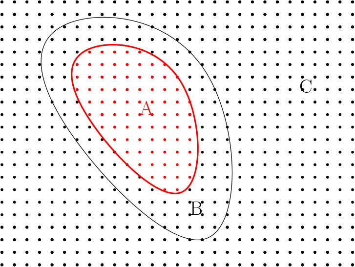
Figure 1: Sketch of the decomposition of $W\subset\mathbb{Z}^{d}$ into $A$, a buffer $B$, and the remaining set $C$.

Corresponding to the tripartition of $W$ we present the spin configurations as $\boldsymbol{\sigma}=(\boldsymbol{\sigma}_{A},\boldsymbol{\sigma}_{B},\boldsymbol{\sigma}_{C})\in\Omega_{A}\times\Omega_{B}\times\Omega_{C}$, and where convenient write the probability associated with $|\psi\rangle$ as

$$|\psi(\boldsymbol{\sigma})|^{2}=p(\boldsymbol{\sigma})=p_{BC}(\boldsymbol{\sigma}_{B},\boldsymbol{\sigma}_{C})\ p_{A}(\boldsymbol{\sigma}_{A}|\boldsymbol{\sigma}_{B},\boldsymbol{\sigma}_{C})\,,$$ (2.1)

in terms of the probability of the variables in $B\sqcup C$, i.e. $p_{BC}(\boldsymbol{\sigma}_{B},\boldsymbol{\sigma}_{C}):=\sum_{\boldsymbol{\sigma}_{A}}p(\boldsymbol{\sigma}_{A},\boldsymbol{\sigma}_{B},\boldsymbol{\sigma}_{C})$, and the conditional probability $p_{A}(\boldsymbol{\sigma}_{A}|\boldsymbol{\sigma}_{B},\boldsymbol{\sigma}_{C})$. The subscripts on such probability functions will be omitted when deemed clear from the context, e.g. $p(\boldsymbol{\sigma}_{B},\boldsymbol{\sigma}_{C})\equiv p_{BC}(\boldsymbol{\sigma}_{B},\boldsymbol{\sigma}_{C})$, etc.

For a pure state $|\psi\rangle$ the reduced state in $A$ is the density matrix

$$\varrho_{A}(\psi)= \sum_{\boldsymbol{\sigma}_{B},\boldsymbol{\sigma}_{C}}p(\boldsymbol{\sigma}_{B},\boldsymbol{\sigma}_{C})\ |\psi_{A}(\boldsymbol{\sigma}_{B},\boldsymbol{\sigma}_{C})\rangle\langle\psi_{A}(\boldsymbol{\sigma}_{B},\boldsymbol{\sigma}_{C})|$$ (2.2)

with the normalized vector $|\psi_{A}(\boldsymbol{\sigma}_{B},\boldsymbol{\sigma}_{C})\rangle\in\mathcal{H}_{A}$, which is indexed by $(\boldsymbol{\sigma}_{B},\boldsymbol{\sigma}_{C})\in\Omega_{B}\times\Omega_{C}$:

$$|\psi_{A}(\boldsymbol{\sigma}_{B},\boldsymbol{\sigma}_{C})\rangle:=\sum_{\boldsymbol{\sigma}_{A}}e^{i\theta(\boldsymbol{\sigma}_{A},\boldsymbol{\sigma}_{B},\boldsymbol{\sigma}_{C})}\sqrt{p(\boldsymbol{\sigma}_{A}\,|\,\boldsymbol{\sigma}_{B},\boldsymbol{\sigma}_{C})}\ |\boldsymbol{\sigma}_{A}\rangle\,.$$ (2.3)

Generically, the rank of the operator in (2.2) reaches $\min\left\{\dim\mathcal{H}_{A},\dim\mathcal{H}_{B\sqcup C}\right\}$. However, for states $|\psi\rangle$ for which the functions defining $|\psi_{A}(\boldsymbol{\sigma}_{B},\boldsymbol{\sigma}_{C})\rangle$ do not vary with $\boldsymbol{\sigma}_{C}$, the rank of $\varrho_{A}(\psi)$ drops to $\dim\mathcal{H}_{B}=\nu^{|B|}$.

Slightly more generally, the rank reduction holds for any state $|\psi\rangle$ for which the corresponding probability and phase functions satisfy the following pair of conditions:

$$\mathrm{(I)}\qquad p(\boldsymbol{\sigma}_{A}\,|\,\boldsymbol{\sigma}_{B},\boldsymbol{\sigma}_{C})=p(\boldsymbol{\sigma}_{A}\,|\,\boldsymbol{\sigma}_{B})\,,$$

$$\mathrm{(II)}\qquad \theta(\boldsymbol{\sigma}_{A},\boldsymbol{\sigma}_{B},\boldsymbol{\sigma}_{C})=\alpha(\boldsymbol{\sigma}_{A},\boldsymbol{\sigma}_{B})\ +\ \gamma(\boldsymbol{\sigma}_{C},\boldsymbol{\sigma}_{B})\,,$$

for some $\alpha:\Omega_{A}\times\Omega_{B}\to\mathbb{R}$ and $\gamma:\Omega_{C}\times\Omega_{B}\to\mathbb{R}$. That is, conditioned on $\boldsymbol{\sigma}_{B}$, the configurations $\boldsymbol{\sigma}_{A}$ and $\boldsymbol{\sigma}_{C}$ are independently distributed (I), and the contributions of $\boldsymbol{\sigma}_{A}$ and $\boldsymbol{\sigma}_{C}$ to the phase function are additive (II). If both conditions hold, then

$$|\psi_{A}(\boldsymbol{\sigma}_{B},\boldsymbol{\sigma}_{C})\rangle=e^{i\gamma(\boldsymbol{\sigma}_{C},\boldsymbol{\sigma}_{B})}\Big{[}\sum_{\boldsymbol{\sigma}_{A}}e^{i\alpha(\boldsymbol{\sigma}_{A},\boldsymbol{\sigma}_{B})}\sqrt{p(\boldsymbol{\sigma}_{A}\,|\,\boldsymbol{\sigma}_{B})}\,|\boldsymbol{\sigma}_{A}\rangle\Big{]}\,=:e^{i\gamma(\boldsymbol{\sigma}_{C},\boldsymbol{\sigma}_{B})}|\phi_{A}(\boldsymbol{\sigma}_{B})\rangle\,,$$ (2.5)

and thus (2.2) reduces to the lower-rank expression

$$\varrho_{A}(\psi)=\sum_{\boldsymbol{\sigma}_{B}}p(\boldsymbol{\sigma}_{B})\ |\phi_{A}(\boldsymbol{\sigma}_{B})\rangle\langle\phi_{A}(\boldsymbol{\sigma}_{B})|\,.$$ (2.6)

The above observation leads us to consider as potential approximations of $|\psi\rangle$ state vectors of the form

$$\boxed{|\psi_{(B)}\rangle:=\sum_{\boldsymbol{\sigma}}e^{i[\alpha(\boldsymbol{\sigma}_{A},\boldsymbol{\sigma}_{B})\ +\ \gamma(\boldsymbol{\sigma}_{C},\boldsymbol{\sigma}_{B})]}\sqrt{p(\boldsymbol{\sigma}_{B})\,p(\boldsymbol{\sigma}_{C}\,|\,\boldsymbol{\sigma}_{B})\,p(\boldsymbol{\sigma}_{A}\,|\,\boldsymbol{\sigma}_{B})}\ |\boldsymbol{\sigma}\rangle\,,}$$ (2.7)

with phase functions $\alpha:\Omega_{A}\times\Omega_{B}\to\mathbb{R}$, $\gamma:\Omega_{C}\times\Omega_{B}\to\mathbb{R}$, which will be variationally selected, and the conditional probabilities of the given state $|\psi\rangle$. One should note the absence of $\boldsymbol{\sigma}_{C}$ in the last conditional probability term in (2.7), in which it differs from that of $|\psi\rangle$. Thus the approximation generically involves changes in both the phase and the amplitude.

For the modified vectors the assumptions (I) and (II) are satisfied, and consequently $\varrho_{A}(\psi_{(B)})$ is given by (2.6). Hence, in contrast to $\varrho_{A}(\psi)$, the induced state $\varrho_{A}(\psi_{(B)})$ is guaranteed to satisfy

$$S\big{(}\varrho_{A}(\psi_{(B)})\big{)}\leq\ln\big{(}\nu^{|B|}\big{)}\propto l\,|\ \partial A|\,,$$ (2.8)

since the rank ($\mathrm{rank}\varrho_{A}(\psi_{(B)})$) is bounded by the number of terms in the sum in (2.6).

Remark 2.1.

For concreteness sake, it may be noted that a simple way to split an additive phase as a sum of the above form is to pick somewhat arbitrarily a configuration $\boldsymbol{\eta}\in\Omega_{W}$ and set $\alpha$ and $\gamma$ as

$$\begin{split}\alpha(\boldsymbol{\sigma}_{A},\boldsymbol{\sigma}_{B})&=\theta(\boldsymbol{\sigma}_{A},\boldsymbol{\sigma}_{B},\boldsymbol{\eta}_{C})-\theta(\boldsymbol{\eta}_{A},\boldsymbol{\sigma}_{B},\boldsymbol{\eta}_{C})]\\ \gamma(\boldsymbol{\sigma}_{C},\boldsymbol{\sigma}_{B})&=\theta(\boldsymbol{\eta}_{A},\boldsymbol{\sigma}_{B},\boldsymbol{\sigma}_{C})\,.\end{split}$$ (2.9)

In a purely additive case, as in (1.9), the sum $\alpha+\gamma$ depends on $\boldsymbol{\eta}$ only through the terms which link directly to both $\boldsymbol{\sigma}_{A}$ and $\boldsymbol{\sigma}_{C}$. In the absence of such, this injection of $\boldsymbol{\eta}$ is for convenience only, its selection having no effect on the analysis.

3 Fidelity bounds

The next question to consider is the degree to which $\varrho_{A}(\psi_{(B)})$ approximates the state of our original interest $\varrho_{A}(\psi\big{)}$. We recall that states’ proximity in trace-norm (denoted $\|\cdot\|_{1}$) is related, via the Fuchs-van de Graaf inequalities [31], to their fidelity $F(\varrho,\sigma):=\left\|\sqrt{\varrho}\sqrt{\sigma}\right\|_{1}^{2}$:

$$1-\sqrt{F(\varrho,\sigma)}\leq\tfrac{1}{2}\|\varrho-\sigma\|_{1}\leq\sqrt{1-F(\varrho,\sigma)}\,$$ (3.1)

In case the two states in $A$ are restrictions of a pair of pure states, by Uhlmann’s principle [52] the fidelity can be estimated through the progenitor state’s global overlap:

$$1-F(\varrho_{A}(\psi),\varrho_{A}(\psi_{(B)})\leq 1-\left|\langle\psi|\psi_{(B)}\rangle\right|^{2}\,.$$ (3.2)

Our upper bounds on the right side will involve two terms, quantifying the deviation of $|\psi\rangle$ from the two idealized conditions listed above as (I) and (II), which do hold for $|\psi_{(B)}\rangle$.

(I)  To address the degree of the correlations in $p(\boldsymbol{\sigma})$ between $\boldsymbol{\sigma}_{A}$ and $\boldsymbol{\sigma}_{C}$, when both are conditioned on the configuration $\boldsymbol{\sigma}_{B}$ of the buffer, we shall use the following terminology and notation.

Without yet conditioning on $B$, we denote by ${\delta}(A\,|\,C)$ the variational difference between the probability distribution of $(\boldsymbol{\sigma}_{A},\boldsymbol{\sigma}_{C})$ and the independent product of the corresponding marginals:

$${\delta}(A\,|\,C) :=\frac{1}{2}\sum_{\boldsymbol{\sigma}_{A},\boldsymbol{\sigma}_{C}}\big{|}p(\boldsymbol{\sigma}_{A},\boldsymbol{\sigma}_{C})-p(\boldsymbol{\sigma}_{A})p(\boldsymbol{\sigma}_{C})\big{|}$$ (3.3)

$$=\sum_{\boldsymbol{\sigma}_{C}}p(\boldsymbol{\sigma}_{C})\sum_{\boldsymbol{\sigma}_{A}}\big{[}p(\boldsymbol{\sigma}_{A}|\boldsymbol{\sigma}_{C})-p(\boldsymbol{\sigma}_{A})\big{]}_{+}\,.$$

with $\big{[}\cdot\big{]}_{+}$ denoting the positive part. Of more direct relevance for our analysis is the following averaged conditional version of the above:

$${\delta}_{B}(A\,|\,C) :=\sum_{\boldsymbol{\sigma}_{B},\boldsymbol{\sigma}_{C}}p(\boldsymbol{\sigma}_{B},\boldsymbol{\sigma}_{C})\sum_{\boldsymbol{\sigma}_{A}}\left[p(\boldsymbol{\sigma}_{A}|\boldsymbol{\sigma}_{C}\boldsymbol{\sigma}_{B})-p(\boldsymbol{\sigma}_{A}|\boldsymbol{\sigma}_{B})\right]_{+}\!$$

$$\equiv\sum_{\boldsymbol{\sigma}_{B}}p(\boldsymbol{\sigma}_{B})\,{\delta}_{\boldsymbol{\sigma}_{B}}(A\,|\,C)$$ (3.4)

where ${\delta}_{\boldsymbol{\sigma}_{B}}$ refers to the ${\delta}(A\,|\,C)$-measure of correlation in the joint distribution of $(\boldsymbol{\sigma}_{A},\boldsymbol{\sigma}_{C})$ conditioned on the specified value of $\boldsymbol{\sigma}_{B}$.

These definitions extend naturally to mutually disjoint $A,B,C\subset W$, whose union does not exhaust $W$. Section 6 includes a more detailed discussion of this quantity as well as estimates in specific models. One may briefly note that for classical Gibbs equilibrium measures (1.8) under local interactions ${\delta}_{B}(A\,|\,C)=0$ once the width of the buffer $B$ exceed the interaction’s range. That does not apply to quantum ground states whose Hamiltonians include non-commuting terms, even in the stoquastic case. Still, one may expect that in non-critical states, the buffer-conditioned correlations would be weak, at least on average.

(II)  For an estimate on the degree of deviation from the second condition we denote

$$\vartheta_{B}(A|C):=\inf_{\alpha,\gamma}\ \left\{\sum_{\boldsymbol{\sigma}}p(\boldsymbol{\sigma})\left|1-U_{\alpha,\gamma}(\boldsymbol{\sigma})\right|^{2}\right\}^{\frac{1}{2}}\,,$$ (3.5)

where

$$U_{\alpha,\gamma}(\boldsymbol{\sigma}):=e^{-i\theta(\boldsymbol{\sigma})}\exp\left(i\left[\alpha(\boldsymbol{\sigma}_{A},\boldsymbol{\sigma}_{B})\ +\ \gamma(\boldsymbol{\sigma}_{C},\boldsymbol{\sigma}_{B})\right]\right)$$

and the optimization is over functions $\alpha:\Omega_{A}\times\Omega_{B}\to[0,2\pi]$ and $\gamma:\Omega_{C}\times\Omega_{B}\to[0,2\pi]$.
Since $\Omega_{A},\Omega_{B},\Omega_{C}$ are finite sets, $[0,2\pi]$ is compact and the right side of (3.5) is continuous in the values of these functions, the infimum is a minimum. Hence, there exist optimizing functions $\alpha_{AB},\gamma_{AC}$ for the infimum.

Let us note that for states $|\psi\rangle$, whose phase is an additive function of the form (1.9), the term $\vartheta_{B}(A|C)$ vanishes if the buffer’s width exceeds the range of the kernel $K$. More generally, $\vartheta_{B}(A|C)$ should be small in case the phase $\theta(\boldsymbol{\sigma})$ is presentable as a sum of quasi local terms similar to (1.9), once the buffer’s width exceeds the relevant coherence length by a factor of order $\ln|\partial A|$.

It will be useful to consider also an extension of the above to the case $A$ is a disjoint union of connected components $A_{1},\dots,A_{n}$, separated by disjoint buffers $B_{1},\dots,B_{n}$ from $C:=W\setminus(A\sqcup B)$ (at $B=\sqcup_{j=1}^{n}B_{j}$), as depicted in Figure 2 for $n=2$. In such case, we denote

$$\vartheta_{B_{1},\dots B_{n}}(A_{1},\dots,A_{n}|C):=\inf_{\alpha_{1},\dots,\alpha_{n},\gamma}\ \left\{\sum_{\boldsymbol{\sigma}}p(\boldsymbol{\sigma})\left|1-U_{(\alpha_{j}),\gamma}(\boldsymbol{\sigma})\right|^{2}\right\}^{\frac{1}{2}}\,,$$ (3.6)

where the infimum is now over $\alpha_{j}:\Omega_{A_{j}}\times\Omega_{B_{j}}\to[0,2\pi]$, $j\in\{1,\dots,n\}$, and $\gamma:\Omega_{C}\times\Omega_{B}\to[0,2\pi]$, and

$$U_{(\alpha_{j}),\gamma}(\boldsymbol{\sigma}):=e^{-i\theta(\boldsymbol{\sigma})}\exp\left(i\left[\sum_{j=1}^{n}\alpha_{j}(\boldsymbol{\sigma}_{A_{j}},\boldsymbol{\sigma}_{B_{j}})\ +\ \gamma(\boldsymbol{\sigma}_{C},\boldsymbol{\sigma}_{B})\right]\right)\,.$$

Since optimizers $\alpha_{1},\dots,\alpha_{n},\gamma$ of (3.6), yield bounds by choosing $\alpha=\sum_{j=1}^{n}\alpha_{j}$ and $\gamma$ in (3.5), we have $\vartheta_{B}(A|C)\leq\vartheta_{B_{1},\dots B_{n}}(A_{1},\dots,A_{n}|C)$.

Our general result will be derived through repeated applications of the following fidelity bound.

Theorem 3.1 (Fidelity bound).

For any state vector $|\psi\rangle$ and its approximation $|\psi_{(B)}\rangle$ defined by (2.7) with optimizers $\alpha=\alpha_{AB}$, $\gamma=\gamma_{CB}$ from (3.5):

$$1-|\langle\psi|\psi_{(B)}\rangle|^{2}\leq 2\ {\delta}_{B}(A\,|\,C)+2\ \vartheta_{B}(A|C)\,.$$ (3.7)

Proof.

We start with the estimate

$$\frac{1}{2}\left(1-|\langle\psi|\psi_{(B)}\rangle|^{2}\right)\leq\left|1-\langle\psi|\psi_{(B)}\rangle\right|\,.$$

Expressing $\psi(\boldsymbol{\sigma})=\sqrt{p(\boldsymbol{\sigma})}\exp\left(i\theta(\boldsymbol{\sigma})\right)$ and $p(\boldsymbol{\sigma})=p(\boldsymbol{\sigma}_{A}|\boldsymbol{\sigma}_{C}\boldsymbol{\sigma}_{B})\,\,p(\boldsymbol{\sigma}_{C}|\boldsymbol{\sigma}_{B})\,\,p(\boldsymbol{\sigma}_{B})$ in terms of conditional probabilities, we have

$$1-\langle\psi|\psi_{(B)}\rangle= \ \sum_{\boldsymbol{\sigma}}p(\boldsymbol{\sigma}_{B},\boldsymbol{\sigma}_{C})\sqrt{p(\boldsymbol{\sigma}_{A}|\boldsymbol{\sigma}_{B},\boldsymbol{\sigma}_{C})}$$

$$\qquad\times\left(\sqrt{p(\boldsymbol{\sigma}_{A}|\boldsymbol{\sigma}_{B},\boldsymbol{\sigma}_{C})}-U_{\alpha,\gamma}(\boldsymbol{\sigma})\sqrt{p(\boldsymbol{\sigma}_{A}|\boldsymbol{\sigma}_{B})}\right)\,.$$ (3.8)

Writing $U_{\alpha,\gamma}=1+(U_{\alpha,\gamma}-1)$, we split the sum into two terms. The absolute value of the part, which is free of $U_{\alpha,\gamma}$, is

$$\Big{|}\sum_{\boldsymbol{\sigma}}p(\boldsymbol{\sigma}_{B},\boldsymbol{\sigma}_{C})\sqrt{p(\boldsymbol{\sigma}_{A}|\boldsymbol{\sigma}_{B},\boldsymbol{\sigma}_{C})}\left(\sqrt{p(\boldsymbol{\sigma}_{A}|\boldsymbol{\sigma}_{B},\boldsymbol{\sigma}_{C})}-\sqrt{p(\boldsymbol{\sigma}_{A}|\boldsymbol{\sigma}_{B})}\right)\Big{|}\\ \leq\frac{1}{2}\sum_{\boldsymbol{\sigma}}p(\boldsymbol{\sigma}_{B},\boldsymbol{\sigma}_{C})\left|p(\boldsymbol{\sigma}_{A}|\boldsymbol{\sigma}_{B},\boldsymbol{\sigma}_{C})-p(\boldsymbol{\sigma}_{A}|\boldsymbol{\sigma}_{B})\right|=\delta_{B}(A|C)\,.$$ (3.9)

The inequality is based on the estimates $-[b-a]_{-}\leq\sqrt{b}\ (\sqrt{b}-\sqrt{a})\leq[b-a]_{+}$ for $a,b\geq 0$, together with the fact that the positive and negative part of the sum are equal. This yields the first term in the right side of (3.7).

The absolute value of the second part is estimated with the help of the triangle inequality and the Cauchy-Schwarz inequality for the sum:

$$\Big{|}\sum_{\boldsymbol{\sigma}}p(\boldsymbol{\sigma}_{B},\boldsymbol{\sigma}_{C})\sqrt{p(\boldsymbol{\sigma}_{A}|\boldsymbol{\sigma}_{B},\boldsymbol{\sigma}_{C})\ p(\boldsymbol{\sigma}_{A}|\boldsymbol{\sigma}_{B})}\left(U_{\alpha,\gamma}(\boldsymbol{\sigma})-1\right)\Big{|}$$

$$\leq\sum_{\boldsymbol{\sigma}}p(\boldsymbol{\sigma}_{B},\boldsymbol{\sigma}_{C})\sqrt{p(\boldsymbol{\sigma}_{A}|\boldsymbol{\sigma}_{B},\boldsymbol{\sigma}_{C})\ p(\boldsymbol{\sigma}_{A}|\boldsymbol{\sigma}_{B})}\left|U_{\alpha,\gamma}(\boldsymbol{\sigma})-1\right|$$

$$\leq\Big{(}\sum_{\boldsymbol{\sigma}}p(\boldsymbol{\sigma})\left|U_{\alpha,\gamma}(\boldsymbol{\sigma},\boldsymbol{\eta})-1\right|^{2}\Big{)}^{1/2}\Big{(}\sum_{\boldsymbol{\sigma}}p(\boldsymbol{\sigma}_{B},\boldsymbol{\sigma}_{C})p(\boldsymbol{\sigma}_{A}|\boldsymbol{\sigma}_{B})\Big{)}^{1/2}\ =\ \vartheta_{B}(A|C)\,.$$ (3.10)

This yields the second term in the right side of (3.7). ∎

4 Entropic implications of rapid decorrelation

In this section, we establish two main results: 1. an area-law bound on the entanglement entropy (1.1) of a state $|\psi\rangle$ restricted to $A\subset W$, and 2. a closely related upper bound for the entanglement entropy difference of $|\psi\rangle$ and $|\psi_{(B)}\rangle$.

4.1 Bounding the density operator’s small eigenvalues

Inspecting (1.1) one may note that the entropy of any state $\varrho_{A}$ is strongly affected by the eigenvalues at the lower end of its spectrum. This is conveniently quantified by the distribution-type function

$$\tau_{\varrho_{A}}(N):=\sum_{j>N}\lambda^{\downarrow}_{j}(\varrho_{A})\,,$$ (4.1)

where the sum is over the eigenvalues of $\varrho_{A}$ labeled in decreasing order. Of particular relevance is the rate at which $\tau_{\varrho_{A}}(N)$ vanishes as $N$ increases towards the dimension of the relevant Hilbert space. The following main lemma estimates this quantity through a combination of (3.2) and the fidelity estimate (3.7).

Lemma 4.1.

Given a state $|\psi\rangle$, for any $A\subset W$ and a buffer set $B$, the spectral distribution function of $\varrho_{A}\equiv\varrho_{A}(\psi)$ satisfies

$$\tau_{\varrho_{A}}\big{(}\nu^{|B|}\big{)}\leq 2\ {\delta}_{B}(A\,|\,W\backslash(A\sqcup B))+2\ \vartheta_{B}(A\,|\,W\backslash(A\sqcup B))\,.$$ (4.2)

Proof.

We use the variational characterization of

$$\tau_{\varrho_{A}}(N)=1-\max\left\{\mathrm{tr}\varrho_{A}P_{N}\ |\ P_{N}\,\mbox{orthogonal projection of $\mathrm{rank}\ P_{N}\leq N$}\right\}$$

$$=1-\max\left\{F(\rho_{A},\widehat{\varrho}_{A})\ |\ \mbox{$\widehat{\varrho}_{A}$ is a state on $A$ with $\mathrm{rank}\ \widehat{\varrho}_{A}\leq N$}\right\}.$$ (4.3)

The last equality is based on the following bound of the fidelity of the state $\varrho_{A}$ with a state $\widehat{\varrho}_{A}$ of $\mathrm{rank}\ \widehat{\varrho}_{A}\leq N$. Denoting by $P_{N}$ the orthogonal projection onto the range of $\widehat{\varrho}_{A}$, the Cauchy-Schwarz inequality for the trace norm implies

$$\left\|\sqrt{\rho_{A}}\sqrt{\widehat{\varrho}_{A}}\right\|_{1}^{2}=\left\|\sqrt{\rho_{A}}P_{N}\sqrt{\widehat{\varrho}_{A}}\right\|_{1}^{2}\leq\mathrm{tr}\rho_{A}P_{N}\,\mathrm{tr}\widehat{\varrho}_{A}=\mathrm{tr}\rho_{A}P_{N}\,.$$

Clearly, the inequality is saturated in case $\widehat{\varrho}_{A}$ is proportional to $\varrho_{A}$ times the projection onto its $N$ highest eigenvalues. This establishes (4.1). The stated inequality follows by combining it with the fidelity bound of Theorem 3.1. ∎

The bound (4.2) gives relevance to the following terminology. In what follows, we restrict attention to regular $A\subset W$ in the sense that the volume of a buffer $B_{l}=\{u\in W\backslash A\ |\ d(u,A)\leq l\}$ of arbitrary width $l\in\mathbb{N}$ is bounded by the surface area of $A$ times $l$, i.e.

$$c_{d}\ l\ |\partial A|\leq\left|B_{l}\right|\leq C_{d}\ l\ |\partial A|$$ (4.4)

with some dimension dependent $c_{d},C_{d}\in(0,\infty)$.

Definition 4.2.

Given a decaying function $\varphi:\mathbb{N}\to[0,1]$ we say that a state $|\psi\rangle$ is conditionally $\varphi$-decoupled at rate $\varphi(l)$ beyond distance $l_{0}:\{\mbox{subsets of $W$}\}\to[0,\infty)$, if for any regular $A\subset W$ and any $l\geq l_{0}(A)$:

$${\delta}_{B_{l}}(A\,|\,C_{l})+\vartheta_{B_{l}}(A|C_{l})\leq\varphi(l-l_{0}(A))$$ (4.5)

with $B_{l}=\{u\in W\backslash A\ |\ d(u,A)\leq l\}$ and $C_{l}=W\setminus(A\cup B_{l})$.

Two rate functions of natural interest are:

• exponential: $\varphi(k)=e^{-k/\xi}$, at some $\xi>0$,

• power law: $\varphi(k)=\left(1+k/\xi\right)^{-\alpha}$ at some $\alpha>2$.

The distance function $l_{0}$ plays the role of the length scale at which the $\varphi$-decay sets in. This could be independent of $A$, in which case $l_{0}$ is constant.

4.2 Area-law bound

A single scale application of (4.2) does not yet produce the desired entropy bound since, due to the presence of the logarithm in (1.1), the von Neumann entropy $S(\varrho_{A})$ is not a trace-norm continuous function of the state. A degree of its continuity is provided by the following variant of Fannes’ continuity bound [28, 11], which involves also rank considerations

$$\left|S(\varrho_{A})-S(\widehat{\varrho}_{A})\right|\leq\tfrac{1}{2}\left\|\varrho_{A}-\widehat{\varrho}_{A}\right\|_{1}\left(1+\ln\frac{2\ \mathrm{rank}(\varrho_{A}-\widehat{\varrho}_{A})}{\left\|\varrho_{A}-\widehat{\varrho}_{A}\right\|_{1}}\right).$$ (4.6)

For the reader’s convenience, a proof is included here in Appendix A.

Taking a cure from [1, 16, 8], we work with a sequence of approximating states using buffers $B_{l}$ of increasing width $l\in\mathbb{N}$. Increase in the buffer size allows to prod lower reaches of the spectrum of $\varrho_{A}(\psi)$. By such means we derive the following general entanglement bound.

Theorem 4.3 (General bound).

For a state $|\psi\rangle$, which is conditionally $\varphi$-decoupled beyond distance $l_{0}$, the entanglement entropy corresponding to any regular $A\subset W$ is bounded according to

$$S(\varrho_{A}(\psi))\leq C_{d}\ |\partial A|\left(\ln\nu\right)\left[l_{0}(A)+2\ (1+l_{0}(A))\ I_{1}(0;A)\right]+2I_{2}(0;A),$$ (4.7)

where

$$I_{1}(l;A):=\mkern-10.0mu\sum_{k=l}^{L(A)}\mkern-5.0mu\varphi(k)(1+k),\quad I_{2}(l;A):=\mkern-10.0mu\sum_{k=l}^{L(A)}\mkern-5.0mu\varphi(k)\left(1+\ln\varphi(k)^{-1}\right),$$ (4.8)

with $L(A):=|A|/(c_{d}\ |\partial A|)$ and $c_{d},C_{d}$ are the constants from (4.4).

Proof.

We split the sum in (1.1) into contributions stemming from the summation index in the intervals

$$J_{0}:=\big{[}1,\nu^{|B_{l_{0}}|}\big{]}\,\mbox{and}\,J_{k}:=\big{(}\nu^{|B_{l_{0}+k-1}|},\nu^{|B_{l_{0}+k}|}\big{]}\,\mbox{with $k\geq 1$.}$$

The bound (4.2) and the assumed decay (4.5) is used to control

$$\mu_{k}:=\sum_{j\in J_{k}}\lambda^{\downarrow}_{j}(\varrho_{A})\leq\tau_{\varrho_{A}}\big{(}\nu^{|B_{l_{0}+k-1}|}\big{)}\leq 2\ \varphi(k-1)$$ (4.9)

in case $k\geq 1$. This will be employed to estimate

$$S_{k}\ :=\sum_{j\in J_{k}}\lambda^{\downarrow}_{j}(\varrho_{A})\ln\lambda^{\downarrow}_{j}(\varrho_{A})^{-1}\leq\mu_{k}\ln\frac{|J_{k}|}{\mu_{k}}\leq\mu_{k}\ln\frac{\nu^{|B_{l_{0}+k}|}}{\mu_{k}}.$$ (4.10)

For $k=0$, we use the trivial bound $\mu_{0}:=\sum_{j\in J_{k}}\lambda^{\downarrow}_{j}(\varrho_{A})\leq 1$, which yields $S_{0}\leq|B_{l_{0}}|\ln\nu$. By (4.4), this leads to the first term in the right of (4.7). If $k\geq 1$, we employ (4.9) and (4.10) to further bound

$$S_{k}\leq 2\ \varphi(k-1)\left(\ln\frac{\nu^{|B_{l_{0}+k}|}}{\varphi(k-1)}+1\right),$$

by the monotonicity of $F(x)=x\left(\ln(a/x)+1\right)$ for $0\leq x\leq 1\leq a$. Collecting the contributions to $S(\varrho_{A})=S_{0}+\sum_{k\geq 1}S_{k}$ and noticing that $k$ does not exceed $L(A)$, since the total number of eigenvalues of $\varrho_{A}\equiv\varrho_{A}(\psi)$ is $\nu^{|A|}$, yields the result. ∎

In order to elucidate this general statement, let us add some comments and formulate a simple consequence. In case $A$ is a cube, it is regular and $L(A)$ is proportional to the cube’s edge length. Moreover, power law decay of $\varphi$ with $\alpha>2$ is enough to ensure the convergence of the series corresponding to the sums in (4.8). One may therefore upper bound these sums independently of $A$. We hence arrive at the following statement, which is one of the main results of this work.

Corollary 4.4 (Area-law bound).

For a state $|\psi\rangle$, which is conditionally $\varphi$-decoupled with power law decay with $\alpha>2$ beyond distance $l_{0}$, there is $C\in(0,\infty)$, which is independent of $l_{0}$, such that the entanglement entropy corresponding to any non-empty, regular $A\subset W$ is bounded by

$$S(\varrho_{A}(\psi))\leq C\ |\partial A|\ (1+l_{0}(A))\,.$$ (4.11)

Proof.

Under the assumption of fast algebraic decay with $\alpha>2$, one has

$$I_{1}(0;A)\leq\sum_{k=0}^{\infty}\frac{1+k}{(1+k/\xi)^{\alpha}}<\infty,\qquad I_{2}(0;A)\leq\sum_{k=0}^{\infty}\frac{1+\alpha\ln(1+k/\xi)}{(1+k/\xi)^{\alpha}}<\infty\,.$$

An application of Theorem 4.3 yields the claim. Note that in case $A\neq\emptyset$, the additive constants can be absorbed into the multiplicative constant in the right side of (4.11). ∎

The bound (4.11) describes a strict area law in case the decoupling distance $l_{0}(A)$ is independent of $A$. This applies in particular to stoquastic states with $p$ any (even critical) classical Gibbs probability measure corresponding to a finite range interaction, cf. (1.8). Such states fall into the category of tensor-network states, for which the area-law of the entanglement entropy is well known (cf. [53, 55]). For ground-states of systems such as the quantum Ising model, existing techniques yield $l_{0}(A)\propto\ln|\partial A|$ for general regular $A$, which results in a logarithmically corrected area law unless $d=1$. In case $W$ is a cylindrical set, $W=V\times[1,...,L]$, and $A=V\times\widehat{I}$ with $\widehat{I}\subset I$, transfer matrix techniques enable one to show $l_{0}(A)\propto\xi$ and hence a strict area law.

Our results have some, but only partial, overlap with the following rigorous results that were formulated for different classes of states, under different assumptions and restrictions.

1. The area-law conjecture for ground states is settled for $d=1$ as well as for exactly solvable or non-interacting systems (cf. [27] for a review). In a trailblazing work, Hastings [35] gave a proof for ground states of gapped local Hamiltonians defined over $W\subset\mathbb{Z}$. As emphasized in [16], this proof relies on the decay of correlations of $|\psi\rangle$.

2. For $d=2$, under the assumption of frustration freeness of a gapped local Hamiltonian on $W\subset\mathbb{Z}^{2}$, Anshu, Arad and Vidick [9] devised a technique for constructing an approximate ground state projector based on a so-called detectability argument. Using that, Anshu, Arad and Gosset [8] established an area-law bound with a poly-logarithmic correction in case of ground states and $A\subset W$ cylindrical sets.

Beyond this two-dimensional case, only conditional results with assumptions that do not cover the full non-critical regime are available [43, 21, 15], and the area law is known to fail for some non-regular graphs [2].

Since the Rényi entropy $S_{\alpha}(\varrho):=(1-\alpha)^{-1}\ln\mathrm{tr}\varrho^{\alpha}$, which agrees with the von Neumann entropy for $\alpha=1$, is monotone decreasing in $\alpha\in(0,\infty)$, the above area-law bound extends to all values $\alpha\geq 1$. In particular, this applies to integer values $\alpha\in\{2,3,\dots\}$ in $d=1$, for which Cardy and Calabrese [20] proposed a value of the proportionality constants of the area law related to the central charge and the correlation length of the conformal field theory describing the non-critical ground state, whose entanglement entropy is described.

4.3 Entropy approximations

Arguments used in the proof of Theorem 4.3 also yield the following bound on entropy differences between the state of interest $|\psi\rangle$ and its approximation $|\psi_{(B_{l}})\rangle$ corresponding to a buffer of width $l$.

Theorem 4.5 (General entropy difference).

In the situation of Theorem 4.3 for any $l\geq l_{0}(A)$:

$$\left|S(\varrho_{A}(\psi))-S(\varrho_{A}(\psi_{(B_{l})}))\right|\leq \sqrt{2\varphi(l-l_{0}(A))}\left(1+\ln\frac{\nu^{|B_{l}|}}{\sqrt{2\varphi(l-l_{0}(A))}}\right)$$ (4.12)

$$+2C_{d}|\partial A|\left(\ln\nu\right)(l+1)\ I_{1}(l-l_{0}(A);A)+2I_{2}(l-l_{0}(A);A)\,,$$

with $|\psi_{(B_{l})}\rangle$ as defined in (2.7) with $B\equiv B_{l}$, $C\equiv W\backslash(A\sqcup B_{l})$ and minimizers $\alpha=\alpha_{AB}$, $\gamma=\gamma_{CB}$ from (3.5).

Proof.

We start as in the proof of Theorem 4.3 with $l_{0}$ substituted by $l$. It was proven there that the contributions to $S(\varrho_{A}(\psi))$ from intervals $J_{k}=\big{(}\nu^{|B_{l+k-1}|},\nu^{|B_{l+k}|}\big{]}$ with $k\geq 1$ are bounded according to

$$\sum_{k\geq 1}S_{k}\leq 2C_{d}|\partial A|\left(\ln\nu\right)(l+1)\ I_{1}(l-l_{0}(A);A)+2I_{2}(l-l_{0}(A);A)\,.$$

The proof then proceeds by estimating the difference of $S(\widehat{\varrho}_{A})$ with $\widehat{\varrho}_{A}\equiv\varrho_{A}(\psi_{(B_{l})})$ and $S_{0}=-\sum_{j=1}^{\nu^{|B_{l}|}}\lambda_{j}^{\downarrow}\ln\lambda_{j}^{\downarrow}$, where $\big{(}\lambda_{j}^{\downarrow}\big{)}$ stand for the eigenvalues of $\varrho_{A}\equiv\varrho_{A}(\psi)$ labeled in decreasing order. For that purpose, let $\mu_{j}^{\downarrow}$, $j\in\{1,\dots,\nu^{|B_{l}|}\}$, denote the decreasing eigenvalues of $\widehat{\varrho}_{A}$. Then

$$\frac{1}{2}\Delta_{l} :=\frac{1}{2}\sum_{j=1}^{\nu^{|B_{l}|}}\left|\lambda_{j}^{\downarrow}-\mu_{j}^{\downarrow}\right|\leq\frac{1}{2}\left\|\varrho_{A}-\widehat{\varrho}_{A}\right\|_{1}$$

$$\leq\frac{1}{2}\left\||\psi\rangle\langle\psi|-|\psi_{(B_{l})}\rangle\langle\psi_{(B_{l})}|\right\|_{1}=\sqrt{1-\left|\langle\psi|\psi_{(B_{l})}\rangle\right|^{2}}$$

$$\leq\sqrt{2{\delta}_{B_{l}}(A\ |W\backslash(A\sqcup B_{l}))}\leq\sqrt{2\varphi(l-l_{0})}\,,$$ (4.13)

where we used [12, Lemma IV.3.2], the variational characterization of the trace norm, $\|a\|_{1}=\sup_{\|b\|=1}\left|\mathrm{tr}(ab)\right|$, as well as the Fuchs-van der Graaf inequality (3.1) in the first three inequalities. The last line is from the fidelity bound (3.7) and the assumed decay. The Fannes-type entropy bound from Proposition A.1 thus yields

$$\left|S_{0}-S(\widehat{\varrho}_{A})\right|=\Big{|}\sum_{j=1}^{\nu^{|B_{l}|}}\big{(}\lambda_{j}^{\downarrow}\ln\lambda_{j}^{\downarrow}-\mu_{j}^{\downarrow}\ln\mu_{j}^{\downarrow}\big{)}\Big{|}\leq\frac{1}{2}\Delta_{l}\left(1+\ln\frac{2\,\nu^{|B_{l}|}}{\Delta_{l}}\right)\,.$$ (4.14)

Inserting (4.3) into the right side and using the monotonicity of the functions then yields the first term in the right side of (4.12). ∎

Let us also put this result into context. Applying the trivial bound (2.8) on the entropy of the comparison state, which holds for arbitrary $l\in\mathbb{N}$ and follows from the rank-estimate on $\varrho_{A}(\psi_{(B)})$, Theorem 4.5 essentially implies (4.7). Since the rank of $\varrho_{A}(\psi)$ is unknown, the bound (4.12) does not immediately follow from the Fannes-Audenaert-continuity bounds [28, 11] or any of its relatives [7, 46].

In the subsequent analysis of the mutual information, we need a minor modification of Theorem 4.5 involving the approximation of $\psi$ by the vector $|\psi_{(B_{l})}\rangle$ from (2.7) with phases now optimized according to (3.6). For simplicity, we restrict attention to the case $n=2$, i.e., the phases will be adapted to the decomposition of $A$ into two separated components $A_{1},A_{2}\subset W$, cf. Figure 2. To formulate a bound, we require the following modification of Defintion 4.2.

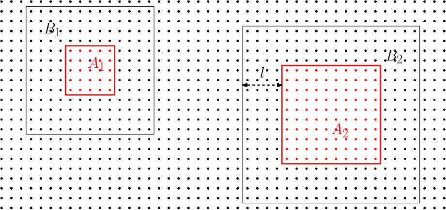
Figure 2: Sketch of the geometric situation in Definition 4.6 and the proof of Theorem 5.1: two cubes $A_{1},A_{2}$ with their buffers $B_{1},B_{2}$ of width $l\approx d(A_{1},A_{2})/3$.

Definition 4.6.

In the situation of Definition 4.2, a state $|\psi\rangle$ is strongly conditionally $\varphi$-decoupled at rate $\varphi(l)$ beyond distance $l_{0}$ if for any $A\subset W$ composed of two disjoint, regular subsets $A_{1},A_{2}$ at distance $d(A_{1},A_{2})\geq 3l$ with their corresponding disjoint buffers $B_{j,l}:=\{u\in W\backslash A\ |\ d(u,A_{j})\leq l\}$ and $l\geq l_{0}(A)$, one has

$${\delta}_{B_{l}}(A\,|\,C_{l})+\delta\left(A_{1}\sqcup B_{1,l}|A_{2}\sqcup B_{2,l}\right)+\vartheta_{B_{1,l},B_{2,l}}(A_{1},A_{2}|C_{l})\leq\varphi(l-l_{0}(A)),$$ (4.15)

where $B_{l}:=\sqcup_{j=1}^{2}B_{j,l}$ and $C_{l}:=W\backslash(A\sqcup B_{l})$.

Remark 4.7.

It will be shown in Theorem 6.1 that in the above situation

$$\delta\left(A_{1}\sqcup B_{1,l}|A_{2}\sqcup B_{2,l}\right)\leq\delta\left(A_{1}|A_{2}\right)+\delta_{B_{1,l}}\left(A_{1}|A_{2}\right)+\delta_{B_{2,l}}\left(A_{1}|A_{2}\right)+\delta_{B_{l}}\left(A_{1}|A_{2}\right)\,.$$ (4.16)

The case $\varphi(k)=e^{-k/\xi}$ at some $\xi>0$, will be referred to as strongly conditionally exponentially decoupled. One may now use the proof of Theorem 4.5 to establish the following variant. In its formulation, we specify a logarithmic decoupling distance $l_{0}(A)\propto\ln|\partial A|$. As explained in Section 6, for ground states of systems with the FKG property such as in the quantum Ising model, present classical statistical mechanics techniques allow to establish exponential decoupling beyond that distance in case one stays away from the ground-state phase transition.

Corollary 4.8 (Entropy difference).

For a state $|\psi\rangle$, which is strongly conditionally exponentially decoupled beyond distance $l_{0}(A)=c\ln|\partial A|$ for some $c\in(0,\infty)$, and any $A\subset W$ composed of two disjoint, regular, non-empty subsets $A_{1},A_{2}$ at distance $d(A_{1},A_{2})\geq 3l$ with $l\geq l_{0}(A)$, there are constants $\widehat{C},\eta,\kappa\in(0,\infty)$, which are independent of $l,l_{0}$ and $A$, such that for all three choices $D\in\{A,A_{1},A_{2}\}$:

$$\left|S(\varrho_{D}(\psi))-S\big{(}\varrho_{D}(\psi_{(B_{l})})\big{)}\right|\leq\widehat{C}\,|\partial A|^{\kappa}\exp\left(-l/\eta\right)\,,$$ (4.17)

with $|\psi_{(B_{l})}\rangle$ as defined in (2.7) with $B\equiv B_{l}:=B_{1,l}\sqcup B_{2,l}$, $C\equiv C_{l}:=W\backslash(A\sqcup B_{l})$ and $\alpha=\alpha_{1}+\alpha_{2}$, and minimizers $\alpha_{1},\alpha_{2}$, $\gamma$ from (3.6).

Proof.

The proof starts by noting that for any of the three reduced states $\varrho_{D}\equiv\varrho_{D}(\psi)$ with $D\in\{A,A_{1},A_{2}\}$, Uhlmann’s bound (3.2) and the fidelity estimate (3.7) still yield for any $l\geq l_{0}(A)$:

$$\tau_{\varrho_{D}}\big{(}\nu^{|B_{l}|}\big{)} \leq 2\ {\delta}_{B_{l}}(A\,|\,W\backslash(A\sqcup B_{l}))+2\ \vartheta_{B_{l}}(A\,|\,C_{l})$$

$$\leq 2\ {\delta}_{B_{l}}(A\,|\,C_{l})+2\ \vartheta_{B_{1,l},B_{2,l}}(A_{1},A_{2}|C_{l})\leq 2\ \varphi(l-l_{0}(A))\,.$$

Applying the same strategy as in Theorem 4.5, we note that (4.12) continues to hold also for the state $|\psi_{(B_{l})}\rangle$ with $\varphi(l)=\exp\left(-l/\xi\right)$. In this case, for any $l\geq l_{0}$:

$$I_{1}(l-l_{0};A) \leq e^{-(l-l_{0}(A))/\xi}\ \sum_{k=0}^{\infty}e^{-k/\xi}(1+k+l-l_{0}(A))\,,$$

$$I_{2}(l-l_{0};A) \leq e^{-(l-l_{0})/\xi}\ \sum_{k=0}^{\infty}e^{-k/\xi}\left[1+(k+l-l_{0}(A))/\xi\right]\,,$$

$$\sqrt{\varphi(l-l_{0})}\left(\ln\frac{\nu^{|B_{l_{0}}|}}{\sqrt{\varphi(l-l_{0})}}+1\right) \leq e^{-(l-l_{0})/(2\xi)}\left(C_{d}\ |\partial A|\ l_{0}\ (\ln\nu)+1+(l-l_{0})/(2\xi)\right)\,.$$

Since $\exp\left(l_{0}(A)/\xi\right)=|\partial A|^{c/\xi}$ and any polynomial in $l$ can be absorbed by peeling of a part of the leading exponential, this implies the result. ∎

5 Mutual information bounds

The above approximation results yield interesting consequences for the mutual information $I_{\psi}(A_{1}:A_{2})$ encoded in a strongly conditionally exponentially decoupled state $|\psi\rangle$ and two disjoint subsets $A_{1},A_{2}\subset W$, cf. Figure 2. Corollary 4.8 allows to approximate each of the entropies entering the definition (1.4) of the mutual information in terms of the entropy of a comparison product state with vanishing mutual information.

Theorem 5.1 (Exponential decay of mutual information).

Let $|\psi\rangle$ be a state, which is exponentially decaying at $l_{0}(A)=c\ln|\partial A|$ for some $c\in(0,\infty)$. Let $A_{1},A_{2}\subset W$ be non-empty squares, which are separated by distance $d(A_{1},A_{2})\geq 3l_{0}(A)$. Then there are constants $C,\kappa,\eta\in(0,\infty)$, which are independent of $A_{1},A_{2}$, such that

$$I_{\psi}(A_{1}:A_{2})\leq C\max\left\{|\partial A_{1}|,|\partial A_{2}|\right\}^{\kappa}\ \exp\left(-d(A_{1},A_{2})/\eta\right)\,.$$ (5.1)

Before spelling out the proof, let us note that the quantum Pinsker inequality (1.6) implies that under the conditions of Theorem 5.1 the correlations of any pair of local observables are exponentially decaying in the observables’ distance - and not only those diagonal in the computational basis.

Moreover, as is evident from the subsequent proof, Theorem 5.1 admits a generalisation to the mutual information of finitely many disjoint squares $A_{1},\dots,A_{n}$.

Proof of Theorem 5.1.

We abbreviate by $\varrho_{A_{1}}\equiv\varrho_{A_{1}}(\psi)$, $\varrho_{A_{2}}\equiv\varrho_{A_{2}}(\psi)$ and $\varrho_{A}\equiv\varrho_{A}(\psi)$ the reduced states of the subsets and their union $A=A_{1}\sqcup A_{2}$. Furthermore, we set $l:=d(A_{1},A_{2})/3$ and denote by

$$B_{j}\equiv B_{j,l}:=\{u\in W\backslash A_{j}\ |\ d(u,A_{j})\leq l\}$$

the buffers of width $l$ around $A_{j}$ with $j\in\{1,2\}$, cf. Figure 2. We also set

$$B\equiv B_{l}:=B_{1,l}\sqcup B_{2,l}\quad\mbox{and}\quad C:=W\backslash(A\sqcup B)\,.$$

The proof then proceeds by a two-step approximation. We first use Corollary 4.8 to approximate each of the three entropies in (1.4) in terms of the respective entropies of the approximating state $|\psi_{(B)}\rangle$ defined in (2.7) with $\alpha=\alpha_{1}+\alpha_{2}$, $\gamma$ the minimizers from (3.6). Corollary 4.8 with $l_{0}(A)=c\ln|\partial A|$ then guarantees that these entropy differences are upper bounded by the right side in (5.1).

In a second step, we approximate the state $|\psi_{(B)}\rangle$ by the state

$$|\psi^{(12)}_{(B)}\rangle:=\sum_{\boldsymbol{\sigma}}\exp\left(i\sum_{j=1}^{2}\alpha_{j}(\boldsymbol{\sigma}_{A_{j}},\boldsymbol{\sigma}_{B_{j}})+i\gamma(\boldsymbol{\sigma}_{C},\boldsymbol{\sigma}_{B})\right)\sqrt{p^{(12)}_{(B)}(\boldsymbol{\sigma})}\ |\boldsymbol{\sigma}\rangle$$ (5.2)

defined in terms of the probability

$$p^{(12)}_{(B)}(\boldsymbol{\sigma}):=p(\boldsymbol{\sigma}_{C}|\boldsymbol{\sigma}_{B})\prod_{j=1}^{2}p(\boldsymbol{\sigma}_{B_{j}})p(\boldsymbol{\sigma}_{A_{j}}|\boldsymbol{\sigma}_{B_{j}})\ \,.$$ (5.3)

The following are straightforward extensions of (2.6) and Theorem 3.1:

1. The reduced state of $|\psi^{(12)}_{(B)}\rangle$ on $A=A_{1}\sqcup A_{2}$ is the product state

   $$\varrho_{A}(\psi^{(12)}_{(B)})=\varrho_{A_{1}}(\psi^{(12)}_{(B)})\otimes\varrho_{A_{2}}(\psi^{(12)}_{(B)})\,,$$ (5.4)

   where $|\varphi_{A_{j}}(\boldsymbol{\sigma}_{B_{j}})\rangle:=\sum_{\boldsymbol{\sigma}_{A_{j}}}e^{i\alpha_{j}(\boldsymbol{\sigma}_{A_{j}},\boldsymbol{\sigma}_{B_{j}})}\sqrt{p(\boldsymbol{\sigma}_{A_{j}}|\boldsymbol{\sigma}_{B_{j}})}\ |\boldsymbol{\sigma}_{A_{j}}\rangle$ with $j\in\{1,2\}$, and

   $$\varrho_{A_{j}}(\psi^{(12)}_{(B)})=\sum_{\boldsymbol{\sigma}_{B_{j}}}p(\boldsymbol{\sigma}_{B_{j}})\ |\varphi_{A_{j}}(\boldsymbol{\sigma}_{B_{j}})\rangle\langle\varphi_{A_{j}}(\boldsymbol{\sigma}_{B_{j}})|\,.$$

2. The fidelity with respect to $|\psi_{(B)}\rangle$ is bounded by

   $$\frac{1}{2}\left(1-\left|\langle\psi^{(12)}_{(B)}|\psi_{(B)}\rangle\right|^{2}\right) \leq\frac{1}{2}\sum_{\boldsymbol{\sigma}_{A},\boldsymbol{\sigma}_{B}}\Big{|}\ p(\boldsymbol{\sigma}_{B})p(\boldsymbol{\sigma}_{A}|\boldsymbol{\sigma}_{B})-\prod_{j=1}^{2}p(\boldsymbol{\sigma}_{B_{j}})p(\boldsymbol{\sigma}_{A_{j}}|\boldsymbol{\sigma}_{B_{j}})\Big{|}$$

   $$\leq\delta\left(A_{1}\sqcup B_{1}|A_{2}\sqcup B_{2}\right)\leq\varphi(l-l_{0}(A))\,.$$ (5.5)

   Note that the phase factors in $|\psi_{(B)}\rangle$ and $|\psi^{(12)}_{(B)}\rangle$ agree and hence drop out in the scalar product.

Since the mutual information of the approximating state $|\psi^{(12)}_{(B)}\rangle$ vanishes,

$$I_{\psi^{(12)}_{(B)}}(A_{1}:A_{2})=0\,,$$

it remains to bound the entropy differences $S\big{(}\varrho_{A}(\psi^{(12)}_{(B)})\big{)}-S\big{(}\varrho_{A}(\psi_{(B)})\big{)}$ and similarly for $A$ replaced by $A_{1}$ and $A_{2}$. This is done with the help of the Fannes’ type bound, Proposition A.1. For its application, we note that the rank of the occurring state differences are bounded by $\dim\mathcal{H}_{B}=\nu^{|B|}=\nu^{|B_{1}|+|B_{2}|}$, where by (4.4), one may further estimate $|B_{j}|\leq C_{d}|\partial A_{j}|\ l$.

The trace distances occuring in the application of Proposition A.1 are estimated by fidelities using (3.1). In turn, each of the fidelities is estimated using Uhlmann’s bound (3.2) in terms of

$$1-\left|\langle\psi^{(12)}_{(B)}|\psi_{(B)}\rangle\right|^{2} \leq 2\delta\left(A_{1}\sqcup B_{1}|A_{2}\sqcup B_{2}\right)$$

$$\leq 2e^{-(l-l0(A))/(3\xi)}=2\ |\partial A|^{c/(3\xi)}e^{-l/(3\xi)}\,.$$ (5.6)

Here, the first inequality is (2) and the second follows from the assumption and the fact that $d(A_{1}\sqcup B_{1},A_{2}\sqcup B_{2})\geq l/3$ by construction. Since $|\partial A|\leq 2\max\left\{|\partial A_{1}|,|\partial A_{2}|\right\}$, this completes the proof. ∎

6 Bounds on conditional dependence

The purpose of this section is to elaborate further on the inter-domain correlation functions introduced in Section 3. These play a central role in our analysis of the probabilistic part, and its applications to specific models.

6.1 General properties

We first collect a number of useful properties of ${\delta}(A\,|\,C)$ defined in (3.3) for arbitrary disjoint subsets $A,C$ among which is last but not least (iii), which is a variant of subadditivity.

Theorem 6.1.

For any probability measure $p$ on a product space $\Omega=\Omega_{0}^{W}$ with $W$ a finite set and $\Omega_{0}$ the range of values of the single “spin variables”, the inter-domain correlation has the following properties for disjoint $A,C,D\subset W$:

1. symmetry: ${\delta}(A\,|\,C)={\delta}(C\,|\,A)$

2. monotonicity: ${\delta}(A\,|\,C)\ \leq\ {\delta}(A\,|\,C\sqcup D)\$

3. sub-cocycle for disjoint $C,D\subset W\setminus A$

   $${\delta}(A\,|\,C\sqcup D)\ \leq\ {\delta}(A\,|\,C)+{\delta}_{C}(A\,|\,D)\,.$$ (6.1)

Proof.

i) The $A\leftrightarrow C$ symmetry is obvious from the defining equation (3.3).

ii) By a known variational characterization of the “total variation” between pairs of probability measures, (3.3) can be restated as

$${\delta}(A\,|\,C)=\frac{1}{2}\max_{\|F_{A,C}\|_{\infty}\leq 1}\sum_{\boldsymbol{\sigma}_{A},\boldsymbol{\sigma}_{C}}F_{A,C}(\boldsymbol{\sigma}_{A},\boldsymbol{\sigma}_{C})\left[p(\boldsymbol{\sigma}_{A}\boldsymbol{\sigma}_{C})-p(\boldsymbol{\sigma}_{A})p(\boldsymbol{\sigma}_{C}))\right]\,,$$ (6.2)

where the maximum is over $F_{A_{C}}:\Omega_{A}\times\Omega_{C}\to[-1,1]$ and attained at $F(\boldsymbol{\sigma}_{A},\boldsymbol{\sigma}_{C}):=\operatorname{sign}[p(\boldsymbol{\sigma}_{A},\boldsymbol{\sigma}_{C})-p(\boldsymbol{\sigma}_{A})p(\boldsymbol{\sigma}_{C})\big{]}$. Monotonicity in $C$ follows, since replacing $\boldsymbol{\sigma}_{C}$ by $\boldsymbol{\sigma}_{C\sqcup D}$ only enlarges the collection of functions over which the maximization is performed.

iii) Regrouping the relevant conditional probabilities into two parts, and applying the triangle inequality, we get:

$$\left|p(\boldsymbol{\sigma}_{A},\boldsymbol{\sigma}_{C},\boldsymbol{\sigma}_{D})-p(\boldsymbol{\sigma}_{A})p(\boldsymbol{\sigma}_{C},\boldsymbol{\sigma}_{D})\right|$$

$$=p(\boldsymbol{\sigma}_{C})\left|p(\boldsymbol{\sigma}_{A},\boldsymbol{\sigma}_{D}|\boldsymbol{\sigma}_{C})-p(\boldsymbol{\sigma}_{A})p(\boldsymbol{\sigma}_{D}|\boldsymbol{\sigma}_{C})\right|$$ (6.3)

$$\leq p(\boldsymbol{\sigma}_{C},\boldsymbol{\sigma}_{D})\left|p(\boldsymbol{\sigma}_{A}|\boldsymbol{\sigma}_{C})-p(\boldsymbol{\sigma}_{A})\right|$$

$$\mkern 150.0mu+p(\boldsymbol{\sigma}_{C})\left|p(\boldsymbol{\sigma}_{A},\boldsymbol{\sigma}_{D}|\boldsymbol{\sigma}_{C})-p(\boldsymbol{\sigma}_{A}|\boldsymbol{\sigma}_{C})p(\boldsymbol{\sigma}_{D}|\boldsymbol{\sigma}_{C})\right|.$$

The sums over configurations of the first and second term on the right coincide with the first and second term on the right side of (6.1), respectively. Thus the claim follows from the inequality in (6.1). ∎

Subadditivity allows to upper bound the conditional inter-domain correlation ${\delta}_{B}(A\,|\,C)$ in terms of sums of domain-to-point correlations ${\delta}_{D}(A\,|\,\{u\})$ with suitable $D\supset B$. It is therefore interesting to note that the latter quantity is upper bounded in terms of an averaged conditional total variation of two measures, which compares the influence under the flip of a single variable. Specifically, for disjoint $A,B,\{u\}\subset W$, we set

$$\overline{{\mathrm{TV}}}_{\boldsymbol{\sigma}_{B}}(A|\{u\}):=\sum_{\sigma_{u},\widehat{\sigma}_{u}\in\Omega_{0}}p(\sigma_{u}|\boldsymbol{\sigma}_{B})p(\widehat{\sigma}_{u}|\boldsymbol{\sigma}_{B})\ {\mathrm{TV}}_{\boldsymbol{\sigma}_{B}}(A;\sigma_{u},\widehat{\sigma}_{u})$$ (6.4)

with

$${\mathrm{TV}}_{\boldsymbol{\sigma}_{B}}(A;\sigma_{u},\widehat{\sigma}_{u}):=\frac{1}{2}\sum_{\boldsymbol{\sigma}_{A}}\left|p(\boldsymbol{\sigma}_{A}|\boldsymbol{\sigma}_{B}\sigma_{u})-p(\boldsymbol{\sigma}_{A}|\boldsymbol{\sigma}_{B}\widehat{\sigma}_{u})\right|$$ (6.5)

In case $B=\emptyset$ and for Gibbs measures $p$, the exponential decay in the distance of $A$ to $u$ of the uniform bound $\sup_{\sigma_{u},\widehat{\sigma}_{u}}{\mathrm{TV}}_{\boldsymbol{\sigma}_{B}}(A;\sigma_{u},\widehat{\sigma}_{u})$ of this total variation is one of the 12 equivalent characterisations (’Condition IIIa’) of the measure’s ’high-temperature’ regime in Dobrushin and Shlosman seminal work [24].

Lemma 6.2.

In the situation of Theorem 6.1 for any disjoint $A,B\subset W$ and $u\in W\backslash(A\sqcup B)$:

$${\delta}_{B}(A,\{u\})\leq\sum_{\boldsymbol{\sigma}_{B}}p(\boldsymbol{\sigma}_{B})\ \overline{{\mathrm{TV}}}_{\boldsymbol{\sigma}_{B}}(A|\{u\})\,.$$ (6.6)

Proof.

This is a simple consequence of the representation

$$p(\boldsymbol{\sigma}_{A}|\boldsymbol{\sigma}_{B}\sigma_{u})-p(\boldsymbol{\sigma}_{A}|\boldsymbol{\sigma}_{B})=\sum_{\widehat{\sigma}_{u}}p(\widehat{\sigma}_{u}|\boldsymbol{\sigma}_{B})\left[p(\boldsymbol{\sigma}_{A}|\boldsymbol{\sigma}_{B}\sigma_{u})-p(\boldsymbol{\sigma}_{A}|\boldsymbol{\sigma}_{B}\widehat{\sigma}_{u})\right]\,,$$

the triangle inequality and the definition (3) of ${\delta}_{B}(A|\{u\})$. ∎

6.2 Relation to correlation function using the FKG property

When applicable, the FKG inequality provides a useful tool for deducing decoupling estimates from the decay rate of the two-point spin-spin correlation function. In its statement we refer to real valued functions on $\mathbb{R}^{n}$ as monotone increasing iff they are so in the component-wise sense.

Definition 6.3.

A probability measure $\mu$ on a product space $\Omega_{0}^{W}$, over a finite set $W$ and based space $\Omega_{0}\subset\mathbb{R}$, is said to have the positive association property if for any pair of increasing, bounded functions $f,g:\Omega_{0}^{W}\to\mathbb{R}$:

$$\langle f\,g\rangle_{\mu}-\langle f\rangle_{\mu}\langle g\rangle_{\mu}\geq 0\,,$$ (6.7)

Furthermore, if this condition holds also for the averages conditioned on prescribed values of the local variables over arbitrary subset $B\subset W$, the probability is said to have the strong positive association property. The latter is also referred to as Fortuin-Kasteleyn-Ginibre (FKG) property.

The FKG property is known to apply to a number of models of interest in statistical mechanics [32]. Included in this class is the classical Ising model and also the quantum ferromagnetic Ising model with the Hamiltonian (1.10) at any $b\geq 0$, and $h\in\mathbb{R}$. For such a system of qubits the following result allows to simplify the verification of the decay of the probability part in Definition 4.2.

Theorem 6.4.

Given a probability $p$ with the FKG property defined over the space of binary configurations $\{+1,-1\}^{W}$:

1. for disjoint $A,B,\{u\}\subset W$:

   $${\delta}_{B}(A\,|\,\{u\})\leq\frac{1}{4}\sum_{a\in A}\langle\sigma_{a};\sigma_{u}\rangle_{B}\,,$$ (6.8)

   where ${\delta}_{B}$ is the conditioned inter-domain correlation defined by (3),

   $$\langle\sigma_{a};\sigma_{u}\rangle_{B}:=\sum_{\boldsymbol{\sigma}_{B}}p(\boldsymbol{\sigma}_{B})\ \langle\sigma_{a};\sigma_{u}\rangle_{\boldsymbol{\sigma}_{B}}\,,$$ (6.9)

   and $\langle\sigma_{a};\sigma_{u}\rangle_{\boldsymbol{\sigma}_{B}}:=\langle\sigma_{u}\sigma_{v}\rangle_{\boldsymbol{\sigma}_{B}}-\langle\sigma_{u}\rangle_{\boldsymbol{\sigma}_{B}}\langle\sigma_{v}\rangle_{\boldsymbol{\sigma}_{B}}$ with the subscript indicating that the expectation values are with respect to the conditional probability $p(\cdot|\boldsymbol{\sigma}_{B})$, conditioned on the value of $\boldsymbol{\sigma}_{B}$.

2. for disjoint $A,B,C\subset W$, the conditional correlation defined in (3) satisfies

   $${\delta}_{B}(A\,|\,C)\leq\frac{1}{4}\sum_{u\in A,v\in C}K_{B}(u,v)\,.$$ (6.10)

   with

   $$K_{B}(u,v):=\max_{D\supset B}\max_{\boldsymbol{\sigma}_{D}}\ \langle\sigma_{u};\sigma_{v}\rangle_{\boldsymbol{\sigma}_{D}}\,.$$ (6.11)

Proof.

1.  We start from (6.6). In the binary case, abbreviating by $p_{\boldsymbol{\sigma}_{B}}(\pm):=p(\sigma_{u}=\pm|\boldsymbol{\sigma}_{B})$, we have

$$\overline{{\mathrm{TV}}}_{\boldsymbol{\sigma}_{B}}(A|\{u\})=p_{\boldsymbol{\sigma}_{B}}(+)\ p_{\boldsymbol{\sigma}_{B}}(-){{\mathrm{TV}}}_{\boldsymbol{\sigma}_{B}}(A),$$

with

$${{\mathrm{TV}}}_{\boldsymbol{\sigma}_{B}}(A) :=\frac{1}{2}\sum_{\boldsymbol{\sigma}_{A}}\left|p(\boldsymbol{\sigma}_{A}|\boldsymbol{\sigma}_{B}\sigma_{u}=1)-p(\boldsymbol{\sigma}_{A}|\boldsymbol{\sigma}_{B}\sigma_{u}=-1)\right|$$

$$=\min\left\{\mathbb{P}\left(\boldsymbol{\sigma}_{A}^{(1)}\neq\widetilde{\boldsymbol{\sigma}}_{A}^{(2)}\right)\ \big{|}\ \mbox{couplings with $\boldsymbol{\sigma}_{A}^{(1)}\rightsquigarrow\boldsymbol{\sigma}_{A}^{+},\boldsymbol{\sigma}_{A}^{(2)}\rightsquigarrow\boldsymbol{\sigma}_{A}^{-}$}\right\}\,.$$

where, by a generally valid formula of the total variation, the minimum is over probability distributions $\mathbb{P}$ of pairs $(\boldsymbol{\sigma}_{A}^{(1)},\boldsymbol{\sigma}_{A}^{(2)})$ with the marginals indicated indicated by $\rightsquigarrow$. Here $\boldsymbol{\sigma}_{A}^{\pm}$ denote the random variables conditioned on $\boldsymbol{\sigma}_{B}$ and $\sigma_{u}=\pm 1$.

Under the assumed strong positive association property of the measure, the Strassen-Holley theorem [38] assures the existence of couplings which are monotone in the sense that for almost every joint realisation of the pair

$$\sigma_{a}^{(1)}\geq\sigma_{a}^{(2)}\quad\mbox{for all $a\in A$}\,.$$ (6.12)

Using any such coupling we get:

$$\mathbb{P}\big{(}\boldsymbol{\sigma}_{A}^{(1)}\big{)}\neq\boldsymbol{\sigma}_{A}^{(2)}\big{)} \leq\mathbb{E}\left(\sum_{a\in A}(\sigma_{a}^{(1)}-\sigma_{a}^{(2)})/2\right)$$

$$=\frac{1}{2}\sum_{\boldsymbol{\sigma}_{A}}M_{A}(\boldsymbol{\sigma}_{A})\big{[}p(\boldsymbol{\sigma}_{A}|\boldsymbol{\sigma}_{B}\sigma_{u}=+1)-p(\boldsymbol{\sigma}_{A}|\boldsymbol{\sigma}_{B}\sigma_{u}=+1)\big{]}$$

in terms of the function $M_{A}(\boldsymbol{\sigma}_{A}):=\sum_{a\in A}\sigma_{a}$.

The above difference also appears in the following expansion for the covariance $\langle M_{A};\sigma_{u}\rangle_{\boldsymbol{\sigma}_{B}}$ where the average is with respect to the conditional distribution $p(\boldsymbol{\sigma}_{A},\sigma_{u}|\boldsymbol{\sigma}_{B})$. That is easily seen by processing a duplicate distribution of an independent pair $(\boldsymbol{\sigma}_{A},\sigma_{u})$, $(\widehat{\boldsymbol{\sigma}}_{A},\widehat{\sigma}_{u})$ of the same distribution:

$$\langle M_{A};\sigma_{u}\rangle_{\boldsymbol{\sigma}_{B}}$$

$$=\frac{1}{2}\sum_{\sigma_{u},\widehat{\sigma}_{u}}\sum_{\boldsymbol{\sigma}_{A},,\widehat{\boldsymbol{\sigma}}_{A}}p(\boldsymbol{\sigma}_{A},\sigma_{u}|\boldsymbol{\sigma}_{B})\ p(\widehat{\boldsymbol{\sigma}}_{A},\widehat{\sigma}_{u}|\boldsymbol{\sigma}_{B})\left[M_{A}(\boldsymbol{\sigma}_{A})-M_{A}(\widehat{\boldsymbol{\sigma}}_{A})\right]\left[\sigma_{u}-\widehat{\sigma}_{u}\right]$$

$$=2\,p_{\boldsymbol{\sigma}_{B}}(+)\ p_{\boldsymbol{\sigma}_{B}}(-)\sum_{\boldsymbol{\sigma}_{A}}M_{A}(\boldsymbol{\sigma}_{A})\big{[}p(\boldsymbol{\sigma}_{A}|\sigma_{u}=+1)-p(\boldsymbol{\sigma}_{A}|\sigma_{u}=+1)\big{]}$$ (6.13)

This completes the proof of the first item.

2.  Iterating (6.1) one learns that for any monotone sequence $C_{0}:=B\subset C_{1}...\subset C_{k}=:C$, one has:

$${\delta}_{B}(A\,|\,C)\ \leq\ \sum_{j=1}^{k}{\delta}_{C_{j-1}}(A\,|\,C_{j}\setminus C_{j-1})$$ (6.14)

In particular, the above applies to sequential decompositions of $C$ with single site increments, $C_{j}=C_{j-1}\cup\{u_{j}\}$, in which case by (6.8) and the definition (6.11) of the influence kernel $K_{B}$:

$${\delta}_{C_{j-1}}(A\,|\,\{u_{j}\})\leq\frac{1}{4}\sum_{a\in A}\sum_{\boldsymbol{\sigma}_{C_{j-1}}}p(\boldsymbol{\sigma}_{C_{j-1}})\ \langle\sigma_{a};\sigma_{u_{j}}\rangle_{\boldsymbol{\sigma}_{C_{j-1}}}\leq\frac{1}{4}\sum_{a\in A}K_{B}(a,u_{j})\,.$$

Inserting this estimate into (6.14), produces (6.10). ∎

7 Application to the quantum Ising model

The model and its phase transitions were outlined in the introduction. Its ground state expectation value functional can be presented as

$$\langle O\rangle^{(W)}=\lim_{\beta\to\infty}\frac{\mathrm{tr}\ O\,e^{-\beta H}}{\mathrm{tr}e^{-\beta H}}$$ (7.1)

with $H$ given by (1.10) acting on $\mathcal{H}_{W}$. The Hamiltonian includes non-commuting terms. In the computational basis based on $S^{z}$ the terms involving $S^{x}$ act as flip operators. It readily follows that the model is stoquastic in this basis (and also in the $S^{x}$ basis, in whose terms $S_{u}^{z}$ act as flip operators).

The part of $H$ involving $S^{z}$ spins looks identical to the classical Ising spin model over the same lattice. In the natural (Dyson-Trotter-Feynman-Kac) functional representation of the trace in (7.1) the expectation value of functions of $\{S_{u}^{z}\}_{u\in W}$ resemble a Gibbs average over a “time”-dependent spin function $\boldsymbol{\sigma}:W\times[0,\beta]\to\{-1,+1\}$. The latter, other than being formulated over a partly continuous set, resembles the classical Ising model over a $(d+1)$ dimensional set.

As it turns out, the relation extends beyond a vague analogy (cf. [48, 5, 14, 39, 22]): the continuum model on $W\times\mathbb{R}$ may be presented as a week limit of discrete models on $W\times(\varepsilon\mathbb{Z})$, at suitably adjusted couplings (which for “time-wise” neighbour’s coupling diverge as $\varepsilon\downarrow 0$).

Through this similarity and relation, results, which were originally derived for the classical Ising model, have found extensions to the the model’s quantum version. Of direct relevance here are the following statements, in which we focus on the finite- and infinite-volume ground states (corresponding to the free boundary conditions).

1. FKG: Like its classical version [38, 32], the quantum Ising model’s probabilty has the FKG property, in the natural partial order of the stoquastic $S^{z}$ basis. This makes Theorem 6.4 applicable to this model, with its variables $\sigma_{u}$ interpreted as $S^{z}_{u}$.

2. Griffiths correlation inequalities: As stated and discussed in [30, 47], these imply that: i) the finite volume ground states’ correlation functions converge as asserted in (1.11), ii) for each $W\subset\mathbb{Z}^{d}$ the ground states’ spin-spin correlation function (of $S^{z}$) is dominated by its infinite volume limit. In the notation of (1.11):

   $$\langle S^{z}_{u}S^{z}_{v}\rangle^{(W)}\leq\langle S^{z}_{u}S^{z}_{v}\rangle^{(\mathbb{Z}^{d})}\,.$$ (7.2)

3. Sharpness of the phase transition: For the QIM it was proven by Björnberg and Grimmett [14] that for any dimension $d\geq 1$ and ferromagnetic coupling $J=\{J_{x-y}\}\not\equiv 0$, there is a finite $b_{c}$ at which the model undergoes a quantum phase transition, as described above (1.12). In particular, for all $b>b_{c}$, the unique ground state exhibits exponential decay at a finite correlation length ($\xi(b)<\infty$)

   $$\langle S^{z}_{u}S^{z}_{v}\rangle^{(\mathbb{Z}^{d})}\leq e^{-|u-v|/\xi(b)}\,.$$ (7.3)

4. Ding-Song-Sun inequality: at any $b$ (omitted in our notation, but to be understood as of common value within the stated relation) and for all finite subsets $D\subset\mathbb{Z}^{d}$ and specified configuration $\boldsymbol{\sigma}_{D}=\{\sigma_{u}\}_{u\in D}$ of $z$-spins:

   $$\langle S^{z}_{u};S^{z}_{v}\rangle_{\boldsymbol{\sigma}_{D}}\leq\langle S^{z}_{u}S^{z}_{v}\rangle\,.$$ (7.4)

   In its classical version, the inequality is a direct implication of the recently formulated Ising inequality, which was presented in [23, Eq. (1.4)]. The validity of its quantum version follows by a continuity argument which, though not spelled, is indicated above. An alternative direct proof, of both classical and quantum versions using the random current approach, is included in [3].

Proof of Theorem 1.1.

As noted above, in the $z$-diagonalising computational basis, the ground states of the quantum Ising model (in finite volumes $W\subset\mathbb{Z}^{d}$ with free boundary conditions) are stoquastic states, with the FKG property.

By the extended Ding-Song-Sun inequality (7.4), for any finite volume and throughout the range of the model’s coupling constants, its ground state’s truncated correlation function, conditioned on arbitrary configuration of the buffer, satisfies:

$$\langle S^{z}_{u};S^{z}_{v}\rangle_{\sigma_{B}}^{(W)}\leq\langle S^{z}_{u}S^{z}_{v}\rangle^{(W)}\leq\langle S^{z}_{u}S^{z}_{v}\rangle^{(\mathbb{Z}^{d})},$$ (7.5)

where the last upper bound holds thanks to the Griffiths inequality. (To avoid confusion, the superscripts here marks the domain over which the model is formulated.)

Combining that with “sharpness of the phase transition”, i.e. exponential decay of correlations in the infinite-volume limit up to the threshold of symmetry breaking, we learn that for any $b>b_{c}$ the above upper bound decays exponentially, as stated in (7.3).

Thus, the kernel, which is defined in (6.11), through maximization of $\langle S^{z}_{u};S^{z}_{v}\rangle_{\sigma_{B}}^{W}$ satisfies

$$K_{B}(u,v)\leq e^{-|u-v|/\xi(b)}$$ (7.6)

at some $\xi(b)<\infty$.

The model’s FKG property makes Theorem 6.4 applicable, boosting the implications of the two point bound. The bound (6.10) allows to conclude that for each $b>b_{c}$, each choice of domains, and $l\geq 1$

$$\delta_{B_{l}}(A|C) \leq \frac{1}{4}\sum_{u\in A,v\in C}\,e^{-|u-v|/\xi(b)}$$ (7.7)

$$\leq C\,|\partial A|\,\xi(b)e^{-l/\xi(b)}\leq e^{-(l-l_{0}(A)/\xi(b)}$$

with $l_{0}(A)=C\ln|\partial A|$.

Combined with Corollary 4.4, this model specific input implies (1.15).

The proof of the claims concerning the mutual information and exponential clustering of observables reduces to an application of (1.6) and Theorem 5.1. Its assumptions are satisfied thanks to (7.7), which by (4.16) also implies that, in the situation of Definition 4.6, the middle term in the left side of (4.15) is exponentially bounded.∎

Let us close with some remarks and open questions.

It seems reasonable to expect that a similar area low bound on the entropy of entanglement is valid also for each of the extremal ($+$ or $-$) ground states throughout the phase which is characterized by symmetry breaking. However in that case while the conditional variational distance $\delta_{\boldsymbol{\sigma}_{B}}(A|C)$ may be small for configurations which are aligned with the sign of the state’s order parameter, it may not be small for some configurations $\sigma_{B}$ which are magnetised in the opposite direction. Still, with $\delta_{B}(A|C)$ being an average of the above, there is a reason to expect the criterion of Corollary 4.4 to be applicable also in that case - provided progress is made on the above point.

A positive, though still insufficient, result in the above direction is the existing proof, by Duminil-Copin, Tassion, and Raoufi [25], that in the classical Ising model in all dimensions the truncated two point function decays exponentially fast at all states except those along the threshold of symmetry breaking [25].

Among the numerous other example of stoquastic Hamiltonians to which the above strategy may be of relevance is the quantum Heisenberg model [26, 50, 51, 49], its ‘flattened’ projection based interactions, studied by related methods in [42, 6, 4] (and by different methods in many other works), and also the ground states of Kitaev’s toric code [40, 49].

Appendix A Fannes’ type bound

The control of entropy differences partially relied on the minor modification (4.6) of Fannes’ well-known entropy bound [28] on the difference of von Neumann entropies of two states $\varrho,\widehat{\varrho}$ in terms of their trace distance and the rank of their difference. Trivially estimating $\mathrm{rank}(\varrho-\widehat{\varrho})$ by the dimension of the Hilbert space on which the states are defined, the following Proposition reduces to [28]. Similarly as the latter and unlike the optimal bound by Audenaert [11], the following bound (which repeats (4.6)) is not sharp.

Proposition A.1.

For any pair of states $\varrho,\widehat{\varrho}$ on a finite-dimensional Hilbert space:

$$\left|S(\varrho)-S(\widehat{\varrho})\right|\leq\frac{1}{2}\left\|\varrho-\widehat{\varrho}\right\|_{1}\left(1+\ln\frac{2\,\mathrm{rank}(\varrho-\widehat{\varrho})}{\left\|\varrho-\widehat{\varrho}\right\|_{1}}\right).$$ (A.1)

For the reader’s convenience, we include a short proof, which is slightly different than the one in  [28] and which we base on the subadditivity of the trace of the following function of non-negative operators. We set $F:[0,\infty)\to[0,\infty)$ with

$$F(x):=\begin{cases}x\left(1+\ln x^{-1}\right),&x\in[0,1],\\ 1,&x>1.\end{cases}$$

Lemma A.2.

For any pair $A,B\geq 0$ of non-negative matrices

$$\mathrm{tr}F(A+B)\leq\mathrm{tr}F(A)+\mathrm{tr}F(B)$$ (A.2)

Proof.

Since $F$ is differentiable on $(0,\infty)$ with derivative $F^{\prime}(x)=\ln x^{-1}$ in case $x\in(0,1)$ and $F^{\prime}(x)=0$ in case $x\geq 0$, we may compute for any $t\in(0,1)$:

$$\frac{d}{dt}\mathrm{tr}F(A+tB)=\mathrm{tr}F^{\prime}(A+tB)B=-\mathrm{tr}B\ln(A+tB)\leq-\left(\mathrm{tr}B\ln t+\mathrm{tr}B\ln B\right).$$

The inequality resulted from the estimate $A+tB\geq tB$ and the operator monotonicity of the logarithm. Integration of the above inequality using $\int_{0}^{1}\ln(t^{-1})dt=1$, yields the first claim. ∎

Proof of Proposition A.1.

We first use monotonicity of $F$ to estimate $\mathrm{tr}F(\varrho)\leq\mathrm{tr}F(A+B)$ with $A=\widehat{\varrho}$ and $B=\left[\varrho-\widehat{\varrho}\right]_{+}$, where the latter denotes the positive part of the difference. Lemma A.2 thus yields:

$$S(\varrho)-S(\widehat{\varrho})=\mathrm{tr}F(\varrho)-\mathrm{tr}F(\widehat{\varrho})\leq\mathrm{tr}F(A+B)-\mathrm{tr}F(\widehat{\varrho})\leq-\mathrm{tr}B\ln B+\mathrm{tr}B.$$

The first term on the right is trivially estimated by $\mathrm{tr}B\ln(\mathrm{rank}B/\mathrm{tr}B)$. Since $\mathrm{tr}(\varrho-\widehat{\varrho})=0$, we have $\mathrm{tr}B=\frac{1}{2}\left\|\varrho-\widehat{\varrho}\right\|_{1}$. This concludes the proof, since the argument holds also for the reversed order of the two states. ∎

Remark A.3.

In the set-up of Lemma A.2, Jensen’s inequality applied to the second term in the right of (A.2) yields

$$\mathrm{tr}F(A+B)\leq\mathrm{tr}F(A)+NF\left(N^{-1}\mathrm{tr}B\right)\,.$$ (A.3)

This inequality holds true more generaly, for any non-decreasing, concave function $F:[0,\infty)\to[0,\infty)$. A proof may be based on an optimal strategy to distribute the total spectral of shift $\mathrm{tr}B$ which the eigenvalues of $A+tB$ undergo as $t$ is increased from $0$ to $1$.

Acknowledgments This work was supported by the Simons Foundation (MA) and by the DFG (SW) under EXC-2111–390814868 and DFG–TRR 352–Project-ID 470903074. SW would like to thank Princeton University for hospitality.

References

- [1] D. Aharonov, I. Arad, U. Vazirani, and Z. Landau. The detectability lemma and its applications to quantum hamiltonian complexity. New Journal of Physics, 13(11):113043, 2011.
- [2] D. Aharonov, A. W. Harrow, Z. Landau, D. Nagaj, M. Szegedy, and U. Vazirani. Local tests of global entanglement and a counterexample to the generalized area law. In 2014 IEEE 55th Annual Symposium on Foundations of Computer Science, pages 246–255, 2014.
- [3] M. Aizenman. Geometric analysis of Ising models, part III. (in preparation).
- [4] M. Aizenman, H. Duminil-Copin, and S. Warzel. Dimerization and Néel order in different quantum spin chains through a shared loop representation. Annales Henri Poincaré, 21(8):2737–2774, 2020.
- [5] M. Aizenman, A. Klein, and C. Newman. Percolation methods for disordered quantum Ising models. In R. Kotecky, editor, Phase Transitions: Mathematics, Physics, Biology, pages 1–26. World Scientific, 1994.
- [6] M. Aizenman and B. Nachtergaele. Geometric aspects of quantum spin states. Communications in Mathematical Physics, 164(1):17–63, 1 1994.
- [7] R. Alicki and M. Fannes. Continuity of quantum conditional information. Journal of Physics A: Mathematical and General, 37(5):L55, 2004.
- [8] A. Anshu, I. Arad, and D. Gosset. An area law for 2d frustration-free spin systems. In Proceedings of the 54th Annual ACM SIGACT Symposium on Theory of Computing, STOC 2022, pages 12–18, New York, NY, USA, 2022. Association for Computing Machinery.
- [9] A. Anshu, I. Arad, and T. Vidick. Simple proof of the detectability lemma and spectral gap amplification. Physical Review B, 93(20):205142, 2016.
- [10] I. Arad, A. Kitaev, Z. Laudau, and U. Vazirani. An area law and sub-exponential algorithm for 1d systems. ArXive:1301.1162, 2013.
- [11] K. M. R. Audenaert. A sharp continuity estimate for the von Neumann entropy. Journal of Physics A: Mathematical and Theoretical, 40(28):8127, 2007.
- [12] R. Bhatia. Matrix analysis, volume 169 of Graduate Texts in Mathematics. Springer New York, 1997.
- [13] J. E. Björnberg. Vanishing critical magnetization in the quantum Ising model. Communications in Mathematical Physics, 337(2):879–907, 2015.
- [14] J. E. Björnberg and G. R. Grimmett. The phase transition of the quantum Ising model is sharp. Journal of Statistical Physics, 136(2):231–273, 2009.
- [15] F. G. S. L. Brandão and M. Cramer. Entanglement area law from specific heat capacity. Physical Review B, 92(11):115134, 2015.
- [16] F: G. S. L. Brandão and M. Horodecki. Exponential decay of correlations implies area law. Communications in Mathematical Physics, 333(2):761–798, 2015.
- [17] O. Bratteli and D.W. Robinson. Operator Algebras and Quantum Statistical Mechanics 1+2. Springer Heidelberg, 1987.
- [18] S. Bravyi, D. P. Divincenzo, R. Oliviera, and B. Terhal. The complexity of stoquastic local hamiltonian problems. Quantum Information and Computation, 8:0361–0385, 2008.
- [19] S. Bravyi and B. Terhal. Complexity of stoquastic frustration-free hamiltonians. SIAM Journal on Computing, 39(4):1462–1485, 2009.
- [20] P. Calabrese and J. Cardy. Entanglement entropy and quantum field theory. Journal of Statistical Mechanics: Theory and Experiment, 2004(06):P06002, 2004.
- [21] J. Cho. Sufficient condition for entanglement area laws in thermodynamically gapped spin systems. Physical Review Letters, 113(19):197204, 2014.
- [22] N. Crawford and D. Ioffe. Random current representation for transverse field Ising model. Communications in Mathematical Physics, 296(2):447–474, 2010.
- [23] J. Ding, J. Song, and R. Sun. A new correlation inequality for Ising models with external fields. Probability Theory and Related Fields, 186(1):477–492, 2023.
- [24] R. L. Dobrushin and S. B. Shlosman. Completely analytical interactions: constructive description. Journal of Statistical Physics, 46:983–1014, 1987.
- [25] H. Duminil-Copin, S. Goswami, and A. Raoufi. Exponential decay of truncated correlations for the Ising model in any dimension for all but the critical temperature. Communications in Mathematical Physics, 374(2):891–921, 2020.
- [26] F. J. Dyson, E. H. Lieb, and B. Simon. Phase transitions in quantum spin systems with isotropic and nonisotropic interactions. Journal of Statistical Physics, 18(4):335–383, 1978.
- [27] J. Eisert, M. Cramer, and M. B. Plenio. Colloquium: Area laws for the entanglement entropy. Reviews of Modern Physics, 82(1):277–306, 2010.
- [28] M. Fannes. A continuity property of the entropy density for spin lattice systems. Communications in Mathematical Physics, 31(4):291–294, 1973.
- [29] S. K. Foong and S. Kanno. Proof of Page’s conjecture on the average entropy of a subsystem. Physical Review Letters, 72(8):1148–1151, 1994.
- [30] S. Friedli and Y. Velenik. Statistical Mechanics of Lattice Systems: A Concrete Mathematical Introduction. Cambridge University Press, 2017.
- [31] C. A. Fuchs and J. van de Graaf. Cryptographic distinguishability measures for quantum mechanical states. IEEE Trans. Inf. Theory, 45:1216–1227, 1999.
- [32] G. R. Grimmett. The Random-Cluster Model. Springer Heidelberg, 2006.
- [33] G. R. Grimmett, T. J. Osborne, and P. F. Scudo. Entanglement in the quantum Ising model. Journal of Statistical Physics, 131(2):305–339, 2008.
- [34] G. R. Grimmett, T. J. J. Osborne, and P. F. Scudo. Bounded entanglement entropy in the quantum Ising model. Journal of Statistical Physics, 178(1):281–296, 2020.
- [35] M. B. Hastings. An area law for one-dimensional quantum systems. Journal of Statistical Mechanics: Theory and Experiment, 2007(08):P08024, 2007.
- [36] M. B. Hastings. How quantum are non-negative wavefunctions? J. Math. Phys., 57:015210, 2016.
- [37] F. Hiai, M. Ohya, and M. Tsukada. Sufficiency, KMS condition and relative entropy in von Neumann algebras. Pac. J. Math., 96:99–109, 1981.
- [38] R. Holley. Remarks on the FKG inequalities. Communications in Mathematical Physics, 36:227–231, 1974.
- [39] D. Ioffe. Stochastic Geometry of Classical and Quantum Ising Models, pages 87–127. Springer Berlin Heidelberg, Berlin, Heidelberg, 2009.
- [40] A. Kitaev. Anyons in an exactly solved model and beyond. Annals of Physics, 321(1):2–111, 2006.
- [41] J. Klassen and B. M. Terhal. Two-local qubit Hamiltonians: when are they stoquastic? Quantum, 3:139, 2019.
- [42] A. Klumper. The spectra of q-state vertex models and related antiferromagnetic quantum spin chains. Journal of Physics A: Mathematical and General, 23(5):809, 1990.
- [43] L. Masanes. Area law for the entropy of low-energy states. Physical Review A, 80(5):052104, 2009.
- [44] M. Ohya and D. Petz. Quantum Entropy and Its Use. Springer New York, 1993.
- [45] D. N. Page. Average entropy of a subsystem. Physical Review Letters, 71(9):1291–1294, 08 1993.
- [46] M. Shirokov. Close-to-optimal continuity bound for the von neumann entropy and other quasi-classical applications of the Alicki–Fannes–Winter technique. Letters in Mathematical Physics, 113(6):121, 2023.
- [47] B. Simon. Phase transitions in the theory of lattice gases. (in preparation).
- [48] S. Suzuki, J. Inoue, and B.K. Chakrabarti. Quantum Ising Phases and Transitions in Transverse Ising Models. Lecture Notes in Physics. Springer Berlin Heidelberg, 2012.
- [49] H. Tasaki. Physics and Mathematics of Quantum Many-Body Systems. Springer Cham, 2020.
- [50] B. Tóth. Improved lower bound on the thermodynamic pressure of the spin 1/2 Heisenberg ferromagnet. Letters in Mathematical Physics, 28(1):75–84, 1993.
- [51] D. Ueltschi. Random loop representations for quantum spin systems. Journal of Mathematical Physics, 54(8):083301, 2013.
- [52] A. Uhlmann. On the Shannon entropy and related functionals on convex sets. Reports on Mathematical Physics, 1(2):174–159, 1970.
- [53] F. Verstraete, M. M. Wolf, D. Perez-Garcia, and J. I. Cirac. Criticality, the area law, and the computational power of projected entangled pair states. Physical Review Letters, 96(22):220601, 2006.
- [54] J. Watrous. The theory of quantum information. Cambridge University Press, 2018.
- [55] M. M. Wolf, F. Verstraete, M. B. Hastings, and J. I. Cirac. Area laws in quantum systems: Mutual information and correlations. Physical Review Letters, 100(7):070502, 2008.