Practical offloading for fine-tuning LLM on commodity GPU via learned subspace projectors

Abstract

Fine-tuning large language models (LLMs) requires significant memory, often exceeding the capacity of a single GPU. A common solution to this memory challenge is offloading compute and data from the GPU to the CPU. However, this approach is hampered by the limited bandwidth of commodity hardware, which constrains communication between the CPU and GPU.

In this paper, we present an offloading framework, LSP-Offload, that enables near-native speed LLM fine-tuning on commodity hardware through learned subspace projectors. Our data-driven approach involves learning an efficient sparse compressor that minimizes communication with minimal precision loss. Additionally, we introduce a novel layer-wise communication schedule to maximize parallelism between communication and computation. As a result, our framework can fine-tune a 1.3 billion parameter model on a 4GB laptop GPU and a 7 billion parameter model on an NVIDIA RTX 4090 GPU with 24GB memory, achieving only a 31% slowdown compared to fine-tuning with unlimited memory. Compared to state-of-the-art offloading frameworks, our approach increases fine-tuning throughput by up to 3.33 times and reduces end-to-end fine-tuning time by 33.1% 62.5% when converging to the same accuracy.

1 Introduction

Recent years have highlighted the remarkable success of billion scale LLMs. Hand-to-hand with task performance improvement are the ever-growing model sizes and the strong demand for powerful computing resources that are only available in high-end clusters. Fortunately, fine-tuning provides common ML practitioners the accessibility to LLMs by allowing them to adapt the pre-trained model to downstream tasks using less onerous computational effort. However, fine-tuning’s memory and compute demand are still daunting. For example, under a default fine-tuning configuration that uses the fp32 data type with the Adam optimizer kingma2014adam , the memory footprint is 16 $\times$ #Parameter, which makes the best consumer GPU devices (e.g., NVIDIA 4090 GPU and AMD 7900XTX with 24GB memory each) only able to hold the smallest LLM (1.5B parameters).

A variety of techniques have been proposed to reduce the memory demand during fine-tuning. A typical solution from system researchers is to offload part of the compute and memory from GPU to CPU, leveraging the fact that commodity laptop CPUs typically have 4x the memory of laptop GPUs and commodity server CPUs can provide 4TBs of memory (per socket). Although offloading is able to scale the trainable model size, large batch sizes are essential to remain efficient despite the limited PCIe bandwidth between CPU and GPU zero-inifity . In fact, we show that training with offloading is inherently bounded by either the CPU-GPU communication or the compute on CPU, especially in the consumer setting characterizing slower CPUs and batch sizes that are constrained by the limited GPU memory. Therefore, offloading itself can hardly save us from the scaling challenge.

Meanwhile, another promising method from ML researchers for memory-reduction is parameter-efficient fine-tuning (PEFT). The key idea of PEFT is to limit the trainable parameters to a carefully designed subspace (e.g., low rank subspace hu2021lora ; zhao2024galore , part of the model guo2020parameter ), so the GPU can train the model without offloading as long as it can hold the parameters and minimal optimizer states for the trainable parameters. However, though more memory-efficient, PEFT methods can suffer from slow convergence or sub-optimal training results due to their overly constrained space for parameter updates.

In this paper, we show how to mitigate the memory challenge by combining both types of approaches. We present LSP-Offload, a novel fine-tuning framework that mitigates the bottlenecks in prior offloading approaches via a new approach for refactoring the offloading process but also trains efficiently via a new approach to constraining the optimization space.

Specifically, to alleviate the compute pressure on CPU as well as the communication overhead back-and-forth between CPU and GPU, we constrain the updates to happen on a periodically changing subspace. Since the updates from different subspaces are projected back and accumulate together in the original space, the model is able to update in the full-rank optimization space. Current approaches hu2021lora ; zhao2024galore for constraining the parameter update space suffer from linear memory and compute complexity that limits them from optimizing in large subspaces. We solve this problem by the introduction of $d$-sparse projectors, sparse embedding matrices that represent a subspace but whose size is independent of the subspace’s size. In this way, given same memory budget as PEFT, we are able to optimize in an arbitrary-size subspace. To further boost the compression quality of the subspace, we adopt a data-driven approach that adapts the subspace to the gradient matrices, which is empirically proven necessary for fast convergence.

Moreover, on the system level, we identify limited parallelism between communication and compute in the SOTA offloading framework zero when run on consumer devices, since their limited GPU memory relative to model size implies that only small batch sizes can be trained efficiently. We improve the SOTA schedule by performing fine-grained communication on the granularity of layers and communicating components of the gradient ahead of time. The new schedule enables us to explore the full parallelism between CPU compute, GPU compute, CPU-to-GPU communication and GPU-to-CPU communication.

In summary, our paper makes following contributions:

• We do an analysis for training LLMs on the single commodity hardware to show that current offloading workflows are fundamentally bounded by either the communication or the CPU’s compute.

• We design LSP-Offload to enable near-native-speed fine-tuning on commodity hardware. The system is built on the key idea of learned subspace projectors, which allows us to optimize on high-dimensional subspaces with constant memory and compute overhead.

• We verify that LSP-Offload can converge at the same rate with native training on the GLUE dataset. Also, in the end-to-end comparison with SOTA offloading framework on the instruction-tuning task, we are able to achieve upto 3.33x higher training throughput and can converge to the same accuracy with 33.1% to 62.5% less of time.

2 Background and Related Work

Memory breakdown for training large language models.

Training a deep learning model requires memory for parameters, activations, and optimizer states. Activations include the intermediate results used in backward propagation. The optimizer states are used by the optimizer to update the parameters. Out of the three, memory for parameters ($M_{param}$) and for the optimizer state ($M_{opt}$) consume most of the memory. When trained with Adam optimizer and half precision, $M_{param}+M_{opt}\approx 8\times\#\text{Parameter}$ bytes, which easily exceeds the single GPU’s memory for billion scale models.

Table 1: Configurations and timings for training/fine-tuning the llama-7B Model on the RTX 4090 and AMD Ryzen Threadripper 3970X CPU. For the Update stage, we measure the fused Adam kernel with thread-level parallelism and SIMD optimizations. For the Bandwidth, we measure the PCIe bandwidth with a pinned memory buffer.

Parameters	Optimizer State	Activations	CPU-GPU Bandwidth	#Layer	GPU Memory
14GB	42GB	8GB	10$\sim$20GB/s	32	24GB
FWD on CPU	BWD on CPU	UPD on CPU	FWD on GPU	BWD on GPU	UPD on GPU
1.61s/layer	3.30s/layer	0.06s/layer	1.7ms/layer	3.5ms/layer	1ms/layer

Memory offloading.

These techniques g10 ; swapadvisor ; zero ; zero-inifity ; zero-offload scale up the training by extending with external memory like the CPU and the disk. Out of these approaches, Zero series are the state-of-the-art approaches for fine-tuning large models. Zero-Offload zero-offload offloads the optimizer states and the update step onto the CPU. Compared to other approaches that only offload the memory to CPU and do all computations on GPU, Zero-Offload achieves the optimal communication volume. Though optimal with regard to the communication volume, we found that Zero’s training is severely bottlenecked by the communication (see § 3). Our work is built on top of the Zero series offloading schedule to make it practical for single GPU training with minimal communication overhead.

Parameter-efficient fine-tuning.

PEFT enables pre-trained models to rapidly adapt to downstream tasks with minimal extra memory required. LoRA hu2021lora is among the most popular PEFT techniques by constraining the updates to weight matrices that lie in a low-rank space. However, recent works lialin2023relora ; valipour2022dylora found LoRA is sensitive to hyperparameter tuning and can struggle with tasks requiring significant change to the base model. To break the low-dimensional constraint of LoRA, Galore zhao2024galore recently explores a similar idea to ours that periodically changes the subspace computed by the singular-value-decomposition. However, both LoRA and Galore have the limitation that their algorithms require extra memory and compute linear with the subspace’s size (rank), which inherently prevent them from tuning on a higher dimensional subspace. Our work mitigates this problem via novel subspace projectors whose compute and memory demands are independent of the subspace size, enabling us to achieve better model accuracy by tuning in a larger subspace.

Other methods for memory-efficient training.

Various approaches such as quantization dettmers2024qlora and gradient checkpointing chen2016training have been proposed to reduce the memory demand for training/fine-tuning LLMs. The quantization approach uses data types with fewer bits for training, and is fully compatible with our techniques. Meanwhile, the gradient checkpointing technique trades computation for memory by recomputing activations during the backward pass. We include this technique in our implementation.

3 Motivation

3.1 Numerical Analysis for Training/Fine-tuning on a Single GPU

In this section, we motivate our work by analyzing the fundamental limits of vanilla offloading on a single consumer-level GPU. We use the example of training/fine-tuning a llama-7B model on an Nvidia RTX 4090 GPU, which can provide only $24/(14+42+8)=37.5\%$ of the required memory (Table 1).

Current offloading techniques can be categorized into two classes: 1) those that offload only memory to CPU, and 2) those that offload both memory and compute to CPU. The first type is represented by swapadvisor ; g10 which perform all compute on GPU while swapping in and out memory on the fly. An example of this type of schedule is shown in Fig. 1.c. However, this type of offloading schedule is inherently bounded by the communication under the following observation:

Observation. Training a model demanding $M_{tot}$ memory on a GPU with only $M_{gpu}$ memory, such that the GPU performs all the computation, requires $\geq M_{tot}-M_{gpu}$ of communication per iteration.

With our example, we need approximately 2.67s communication every iteration for each of CPU-to-GPU and GPU-to-CPU communication, which adds 3.2x overhead compared to the compute on GPU even if the compute and communication are fully overlapped.

The second type of offloading schedule splits the workload across CPU and GPU. Among the forward pass, backward pass, and parameter update, because of CPU’s poor computing power, only the parameter update step (UPD) is suitable to run on the CPU. For example, assigning the forward+backward pass of just one layer to the CPU directly adds 4.9s overhead, which is already 3.21x the GPU compute. Moreover, offloading UPD to CPU means that the 42GB optimizer state can reside on the CPU, enabling larger models like llama-7B to fit in the GPU memory.

Offloading UPD to CPU was first realized in Zero-Offload zero-offload , whose schedule is displayed in Fig. 1.a. In their schedule, $M_{param}$ communication happens every iteration (gradients to CPU, deltas to GPU), which brings the communication overhead to 0.93s, but is still 1.11x the GPU compute time. When there is no overlap between CPU compute and GPU compute, the training slowdown can reach 2.11x.

Moreover, the CPU computation can become the bottleneck for Zero’s schedule. In our example, it takes approximately 1.92s per iteration for parameter update on the CPU. Therefore, when CPU’s compute is not paralleled with the GPU, this slows down the training by 2.14x.

This analysis shows that training/fine-tuning with offloading is computationally inefficient on a consumer device due to fundamental bottlenecks in communication and/or CPU compute. This motivates us to design a lossy (PEFT) algorithm for reduced communication/compute overheads.

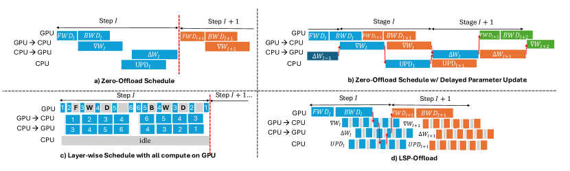
Figure 1: Comparison between current offloading pipelines and LSP-Offload’s overlapped pipeline.

Algorithm 1 Zero-Offload’s Pseudo-code

Input: $M$: GPU model, $S$: Opt. State on CPU, $W$: Weights, $X$: Data

for $t\leftarrow 1$ to $T$ do

     Sample Input $x\sim X$

     $l\leftarrow M.forward(x)$$\triangleright$ FWD on GPU

     $\nabla_{W}l\leftarrow SendToCPU(M.backward(l))$$\triangleright$ Paralleled BWD on GPU and Gradient Offload

     $\Delta W\leftarrow SendToGPU(Update(\nabla_{W}l,S))$$\triangleright$ Paralleled Update on CPU and Delta Upload

     $W\leftarrow W+\eta_{t}\cdot\Delta W$$\triangleright$ on GPU

3.2 Case Study on Zero’s Schedule

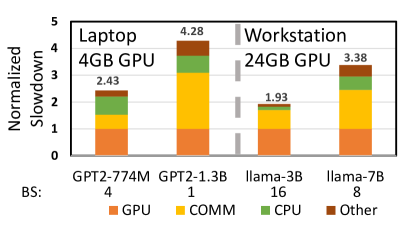
Figure 2: Normalized slowdown of Zero’s schedule. The breakdown for communication (COMM) depicts the additional slowdown due to communication that is not overlapped with GPU compute. Similarly, the CPU compute and Other are additional non-overlapped overheads. The experiments are done using precision fp16 under maximum allowed batch size with gradient checkpointing.

Moreover, prior offload schedules are suboptimal. Here we profile Zero-Offload’s schedule for a more comprehensive view of its performance. We chose two settings for profiling: 1) training a GPT2 model on a 4GB GPU representing the personal laptop, and 2) training a llama model on a 24GB GPU representing the workstation. The slowdown normalized by the GPU compute time is shown in Fig. 2. Under both configurations, Zero’s schedule lowers the training speed by 1.73x to 4.28x. We ascribe the slowdown to the following two reasons.

Communication and CPU compute overhead.

The primary source of overhead comes from the unavoidable high communication volume and slow CPU compute as demonstrated in our previous analysis. Shown in Fig. 2, though Zero is able to overlap part of the GPU/CPU compute with communication, the non-overlapped communication brings 0.61x to 2.09x added slowdown compared to the GPU compute time. For each GPU, the situation is worse for the larger model because the maximum available batch size decreases. When training a 1.3B model on a 4GB GPU, the non-overlapped communication and CPU compute are 2.09x, 0.63x the GPU compute respectively.

Limited parallelism between CPU and GPU, communication and compute.

The second source of overhead comes from Zero’s limited parallelism between compute and communication. Fig. 1.a shows Zero’s standard training pipeline, which is sub-optimal for two reasons: 1) The forward and backward pass on the GPU is not overlapped with the CPU’s compute. This results in significant slowdown when the CPU compute is around the same scale as the GPU’s compute. 2) No overlap exists between the GPU-to-CPU communication and CPU-to-GPU communication. As a result, the duplex PCIe channel, which is able to send and receive data between CPU and GPU in both directions at full bandwidth at the same time, is at least 50% under utilized.

Thus, the per-iteration time is:

$$T_{Zero}^{iter}=T_{FWD}+\max\{T_{BWD},T_{Comm}^{\text{GPU-to-CPU}}\}+\max\{T_{UPD},T_{Comm}^{\text{CPU-to-GPU}}\}$$ (1)

To mitigate the first issue, Zero proposed delayed parameter updates (Fig. 1.b), which use stale parameter values to calculate current gradients, allowing the CPU to perform the previous step’s update at the same time the GPU performs the current step’s forward and backward passes. Though increasing throughput, this method can hurt training accuracy. Also, in order to not incur additional memory for buffering communication, the CPU-to-GPU communication and GPU-to-CPU communication cannot be parallelized.

These limitations motivate us for a layer-wise schedule that enables maximal parallelism between CPU compute, GPU compute, CPU-to-GPU communication and GPU-to-CPU communication.

4 LSP-Offload’s Approach

In this section, we present LSP-Offload, a practical offload framework for a commodity GPU that mitigates the problems identified in §3. We will first introduce our lossy training algorithm for reducing the communication and compute pressure of the gradient update step. Afterwards, we will illustrate our new schedule design for maximized parallelism in the offloading’s schedule.

4.1 Communication/Compute-efficient Parameter Update via Learned Subspace Projectors

As observed in the prior section, the communication and compute complexity of current gradient updates cannot be improved without changes to the training algorithm. Therefore, a “lossy” approach is a necessity for practical offloading. Ideally, the new training algorithm should: 1) reduce the communication amount, 2) reduce the computational complexity for the parameter update on CPU, and 3) converge at the similar rate with the standard training algorithm.

To obtain such an algorithm, we borrow the key idea from the PEFT field that constrains the optimization in a subspace. Specifically, we consider the matrix multiplication operations in the network, which cover over $90\%$ of the parameters in the transformer architecture. Same as the Gradient Low-rank Projection in Galore zhao2024galore , we approximate the gradient by projecting the gradient matrix onto two sets of bases. Mathematically, for the gradient $G\in\mathbb{R}^{m\times n}$ and bases $P\in\mathbb{R}^{m\times s}$ and $Q\in\mathbb{R}^{n\times s}$, where $s\ll\min(m,n)$, the subspace and approximated gradient are given by:

$$S=\{P^{T}AQ\ \in\mathbb{R}^{s\times s}|\ A\in\mathbb{R}^{m\times n}\},\quad\hat{G}:=\mathcal{C}(G)=PP^{T}GQQ^{T}.$$

In this way, we constrain the parameter updates to the subspace $S$, such that only $P^{T}GQ\in\mathbb{R}^{s\times s}$ needs to be communicated every iteration. Therefore, both communication and compute complexity for the parameter update step is reduced from $O(m\cdot n)$ to $O(s^{2})$.

Table 2: Additional time and space complexity of different subspace training methods. $m,n$ are the dimensions of the weight matrix, $s$ is the subspace size, and $d\ll s$ is the number of nonzero values per row in our projectors.

	LoRA hu2021lora	Galore zhao2024galore	LSP-Offload
Time Complexity	$O(mns)$	$O(mns)$	$O(mnd)$
Space Complexity	$O((m+n)s)$	$O((m+n)s)$	$O((m+n)d)$

Next, we need to come up with good bases to represent the subspace, which is our key contribution. As discussed in §3 and shown in Table 2, both LoRA and Galore have $O(mns)$ time complexity and $O((m+n)s)$ space complexity, due to the adaptor matrices LoRA and the dense subspace represented by top eigenvalues in Galore. Suppose we want to optimize in a subspace of size $512$ for the Llama-7B model, this results in an extra $3GB$ of storage in half precision, which is an unignorable $3/14=21\%$ of the parameter memory.

Algorithm 2 LSP-Offload’s training/fine-tuning with learned sparse projectors (simplified version without layer-wise scheduling)

HyperParam: $s$: subspace size. $d$: $d$-sparse projectors. $\gamma\in\mathbb{R}^{+}$. $CheckFreq,threshold$: check frequency and threshold for updating projectors.

procedure UpdateSubspace($G$: the gradient, $P_{old}$, $Q_{old}$: previous projectors)

     $P,Q\leftarrow Initialize(d)$

     Minimize $loss:=\|PP^{T}GQQ^{T}-G\|_{F}^{2}+\gamma\cdot(\|P\|_{F}^{2}+\|Q\|_{F}^{2})$ by SGD.

     $M\in\mathbb{R}^{s\times s}\leftarrow P^{T}P_{old}MQ_{old}Q^{T}$

     $V\in\mathbb{R}^{s\times s}\leftarrow(P^{T}P_{old})^{2}V(Q_{old}Q^{T})^{2}$

     return $P,Q$

procedure Main($M$: GPU model, $\mathcal{D}$: Dataset, $W\in\mathbb{R}^{m\times n}$: Weights, $M,V\in\mathbb{R}^{s\times s}:$ First and second order optimizer state)

     for $t\leftarrow 0$ to $T-1$ do

         Sample $x\sim\mathcal{D}$

         if $t\mod CheckFreq=0$ then$\triangleright$ Periodically check for better projectors

              Calculate gradient $\nabla_{W}f_{S}$ on random sampled subset $S\subset\mathcal{D}$.

              if $\|PP^{T}\nabla f_{S}(W)QQ^{T}-\nabla f_{S}(W)\|_{F}^{2}\geq threshold\cdot\|\nabla f_{S}(W)\|$ then

                  $P,Q\leftarrow$ UpdateSubspace($\nabla_{W}f_{S}$, $P$, $Q$)                        

         $\triangleright$ Note: In full LSP-Offload, these four steps are parallelized using layer-wise scheduling

         $\nabla f_{x}(W)\leftarrow forwardBackward(M,x)$$\triangleright$ FWD+BWD on GPU

         $grad\leftarrow SendToCPU(P^{T}\nabla f_{x}(W)Q)$$\triangleright$ Compress on GPU and gradient offload

         $\Delta_{W}\leftarrow SendToGPU(Update(grad))$$\triangleright$ UPD on CPU and delta upload

         $W\leftarrow W+\eta_{t}P\Delta_{W}Q^{T}$$\triangleright$ Decompress and apply deltas on GPU      

In this work, we propose to solve this problem by using a sparse projector similar to the JL-sparse embedding matrix kane2014sparser whose time and space complexities are independent of the size of the subspace.

Definition 1 (Sparse Projector).

We call the projection bases $P\in\mathbb{R}^{n\times s},Q\in\mathbb{R}^{m\times s}$ a pair of $d$-sparse projectors if both $P,Q$ have $d$ nonzeros values per row.

As shown in Table 2, a pair of $d$-sparse projectors require only $O((m+n)\cdot d)$ memory and the projection operation $P^{T}\cdot A\cdot Q$ can be done efficiently in $O(mnd)$ time.

Next, we describe our training algorithm with the $d$-sparse projector. We denote the loss function as $f(W):=\frac{1}{|\mathcal{D}|}\Sigma_{x\in\mathcal{D}}f_{x}(W)$, where $f_{x}(W)$ is the loss on a specific data point. We denote the loss on a subset $S\subset\mathcal{D}$ as $f_{S}(W):=\frac{1}{|\mathcal{S}|}\Sigma_{x\in\mathcal{S}}f_{x}(W)$.

To find a good $d$-sparse projector pair, we take a check-and-update approach that minimizes the empirical bias of the gradient estimator defined as $\textbf{b}(W)=\mathbb{E}_{x\sim\mathcal{D}}[\mathcal{C}(\nabla f_{x}(W))]-\nabla f(W)$. As shown in Alg. 2, we periodically check the quality of the empirical bias on a sub sampled dataset. When the bias exceeds a certain threshold, we update the subspace to reduce the empirical bias.

Compared to Galore zhao2024galore who perform the update step periodically, our check-and-update mechanism guarantees the quality of the subspace while minimizes the frequency of the update operation.

In terms of convergence, we characterize the quality of the subspace by Assumption 3. Under the assumptions on the norm bound and sparsity of the bias, we are able to show the convergence of our algorithm in The. 1 following the analysis in  stich2020analysis . Compared to vanilla training, the bound for time-to-convergence is increased by a factor of $\frac{1}{1-2c^{2}\alpha^{2}}$. Moreover, only logarithmic-scale samples are needed in the sub-sampled dataset for convergence.

Assumption 1 (Bounded Bias).

There exists $\gamma>0$, such that for any weight $W$ and $x\sim\mathcal{D}$, $\|\mathcal{C}(\nabla f_{x}(W))-\nabla f_{x}(W)\|<\gamma,\|\nabla f_{x}(W)\|<\gamma$.

Assumption 2 (Sparse Bias).

There exists constant $c>0$, such that $\|\textbf{b}(W)\|_{F}<c\|\textbf{b}(W)\|_{2}$ holds for any $W$.

Assumption 3 (Effectiveness of the subspace).

For any subset $S\subset\mathcal{D}$ and fixed constant $0<\alpha<\frac{1}{\sqrt{2}c}$, and any weight matrices $W$, we are able to find a compressor $\mathcal{C}$ such that $\|\mathcal{C}(\nabla f_{S}(W))-\nabla f_{S}(W)\|<\alpha\|\nabla f_{S}(W)\|$.

Theorem 1.

For any $\beta>0,0<\delta<1$, Suppose f is a L-smooth function, under Assumptions 1, 2, 3, and we check every iteration in Alg. 2 with the sub-sampled dataset $S$ of size $\mathcal{O}(\frac{8\gamma^{2}}{3\beta^{2}}\log{\frac{(m+n)T}{\delta}})$, and stepsize $\eta=\frac{1}{L}$, denote $F:=\mathbb{E}[f(W_{0})]-f^{*}$, with probability $1-\delta$,

$$T=\mathcal{O}(\frac{1}{\epsilon})\cdot\frac{LF}{(1-2c^{2}\alpha^{2})}$$

iterations are sufficient to obtain $\min_{t\in[T]}\mathbb{E}\|\nabla f(W_{t})\|^{2}=\mathcal{O}(\epsilon+\frac{2c^{2}\beta^{2}(1+\alpha)^{2}}{1-2c^{2}\alpha^{2}})$.

During the update, we initialize the sparse embedding by first choosing non-zero positions in each row, and then assigning values to them under normal distribution $\mathcal{N}(0,\frac{1}{\sqrt{d}})$, which yields an unbiased estimation of the gradient.

Afterwards, we fix the non-zero positions and optimize the values in the sparse embedding matrix to minimize the empirical bias. We define our loss function as the bias with norm regularization:

$$loss:=\|PP^{T}GQQ^{T}-G\|_{F}^{2}+\gamma\cdot(\|P\|_{F}^{2}+\|Q\|_{F}^{2})$$

Finally, when trained with Adam optimizer, we need to project the old momentum and velocity tensor to the new subspace.

Because we are periodically learning a new pair of $d$-sparse projectors as the training/fine-tuning proceeds, we can fine-tune to higher accuracies than approaches like LoRA that constrain the possible adjustments to the base model.

Algorithm 3 Layer-wise Scheduling

Hyperparameter: $TransitionLayer:$ The layer to change the schedule mode from FirstComeFirstServe to LastComeFirstServe. Others are same as Alg. 2.

for $t\leftarrow 0$ to $T-1$ do

     Sample $x_{0},y\sim\mathcal{D}$

     for $l$ in $layers$ do

         Wait for event $e_{l}$. $\triangleright$ The forward pass happens after the parameter gets updated

         $x_{l}\leftarrow forward(x_{l-1},l,W_{l})$      

     $grad=loss(x_{l},y)$

     $SchMode\leftarrow FCFS$

     for $l$ in $reversed(layers)$ do

         if $l$ is TransitionLayer then

              $SchMode\leftarrow LCFS$          

         $grad,\nabla_{W_{l}}\leftarrow backward(grad,x_{l},l,W_{l})$

         $e_{l}\leftarrow AsyncSchedule(SchMode,\nabla_{W_{l}},Stream_{G2C})$

         $e_{l}\leftarrow AsyncScheduleAfter(e_{l},SchMode,\Delta_{W_{l}}\leftarrow Update(\nabla_{W_{l}}),CPU)$

         $e_{l}\leftarrow AsyncScheduleAfter(e_{l},SchMode,W_{l}\leftarrow W_{l}+\eta\nabla_{W_{l}},Stream_{C2G})$      

4.2 Layer-wise Schedule for Maximal Parallelism

On the system level, we propose a new schedule that solves both issues in Zero’s schedule based on the observation that there is no dependency between different layer’s optimizer update steps. Because of this, we are able to overlap different layers’ GPU compute, CPU-GPU communication in both directions, and the parameter update on the CPU. Alg.3 presents pseudo-code for our new highly-parallel layer-wise schedule. The key idea and its benefits are illustrated in Fig. 1.d. We split the GPU-to-CPU, CPU update, CPU-to-GPU communication into small blocks to unlock the parallelism between layers without the accuracy loss of Zero’s use of stale parameter values. We parallelize the CPU’s and GPU’s compute by executing the deeper layers’ update step on CPU while doing the backward pass of shallower layers on GPU. We also parallelize the double-sided communication by executing deeper layer’s upload step while doing the shallower layer’s offload step. Thus, in our schedule, the critical path of the training can be characterized by:

$$T_{ours}^{iter}=\max\{T_{FWD}+T_{BWD}+T_{Comm}^{layer}+T_{UPD}^{layer},T_{Comm}^{\text{GPU to CPU}},T_{Comm}^{\text{CPU to GPU}},T_{UPD}\}.$$

Compared to Eqn. 1, LSP-Offload is able to reduce the CPU’s involvement in the critical path from the entire parameter update step to the update for only one layer, a 32x improvement for the llama-7B model.

Further, to avoid the deeper layer’s workload from blocking the shallower layer’s computation which involves earlier in the next iteration, we use a heuristic to switch between two schedule mode: $FirstComeFirstServe$(FCFS) and $LastComeFirstServe$(LCFS). When the backward pass begins, FCFS is used first for parallelizing GPU compute and offloading. As the backward pass proceeds, we change the Schedule to LCFS which helps shallower layers get ready for the next pass. We set the switch point to be $TransitionLayer=\#Layer-\frac{T_{BWD}-(T^{layer}_{Offload}+T^{layer}_{Upload}+T^{Layer}_{UPD})}{max\{T^{layer}_{Offload},T^{layer}_{Upload},T^{Layer}_{UPD}\}}$, which is the deepest layer that may block the computation of the first layer.

5 Implementation

We propotyped LSP-Offload as a Python library built on top of Pytorch. LSP-Offload can automatically detect the matrix multiplication modules and replace it with the offloaded version without user’s interference. To achieve best performance, we implemented the fused Adam kernel in Zero-Offload to accelerate the parameter update on CPU. Also, we used the Pinned Memory buffer on CPU to enable fast communication, and used CUDA streams for paralleled communication and computation.

6 Evaluation

In evaluation, we first verify the convergence of the LSP training approach on the GLUE dataset and then evaluate the end-to-end training performance on the instruction-tuning task. Detailed configurations for the experiments are described in the §9.2.

Convergence and Accuracy validation of LSP training on GLUE

First of all, we verify the convergence and accuracy of Alg. 2 by fine-tuning pre-trained RobertA-baseliu2019roberta (117M) model on the GLUE wang2018glue dataset, which is a language understanding task sets that are widely adopted in the fine-tuning’ s evaluationhu2021lora ; zhao2024galore . For hyper parameters, We set both the rank of Galore’ s projector and the non-zero entries per row in the LSP algorithm to be 16. We set the projection space of LSP to be 512. As both Galore and LSP need additional profiling time, we make an end-to-end comparison that allow all candidates to train under an hour’s time budget.

Shown in Fig. 3, for all cases in GLUE, the LSP algorithm is able to converge at the same rate with the full parameter tuning. In fact, as displayed in Tab. 3, LSP is able to outperform full parameter tuning, which indicates constraining the update space can help with the performance. Meanwhile, compared to Galore, we are able to achieve 1% higher averaged accuracy. We attribute this to the LSP algorithm’s larger parameter update space, which is 1024x for this experiment.

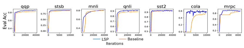
Figure 3: Convergence Validation of LSP by finetuning pre-trained RoBertA-base model on GLUE.

Table 3: Accuracy Validation of LSP by finetuning pre-trained RoBertA-base model on GLUE

	Memory	#Trainable	MNLI	SST2	MRPC	CoLA	QNLI	QQP	SST2	STS-B	Avg
Full Parameter	747M	747M	0.8111	0.934	0.866	0.55	0.904	0.808	0.933	0.884	0.8362625
Galore (Rank = 16)	253M	18K	0.83	0.92	0.88	0.567	0.881	0.852	0.92	0.9	0.84375
LSP (S: 512, d: 16)	253M	18M	0.814	0.917	0.911	0.6165	0.9178	0.8339	0.922	0.91	0.855275

End-to-end evaluation of the LSP-Offload on Alpaca.

Next, we evaluate the end-to-end performance of LSP-Offload by fine-tuning on the instruction-tuning dataset Alpaca alpaca . We perform our evaluation in two settings: 1) fine-tuning the GPT2 (774M) model on a laptop with Nvidia A1000 Laptop GPU (4GB) and Intel Core-i7 12800H CPU (32GB), and 2) fine-tuning a Llama-3B model on commodity workstation with Nvidia RTX 4090 GPU (24 GB) and AMD Ryzen Threadripper 3970X CPU (252GB). We compared LSP-Offload with Zero-Offload for full-parameter tuning, as well as LoRA for PEFT fine-tuning.

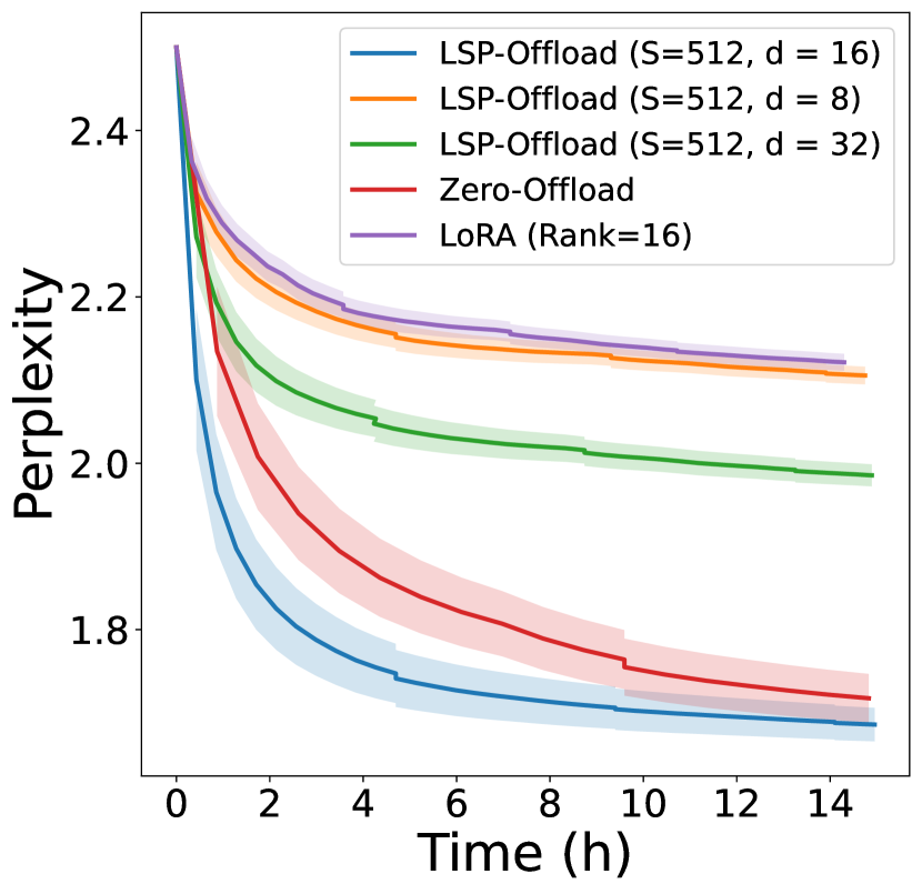
(a) Evaluation PPL. of fine-tuning GPT2-774M w/ the laptop GPU.

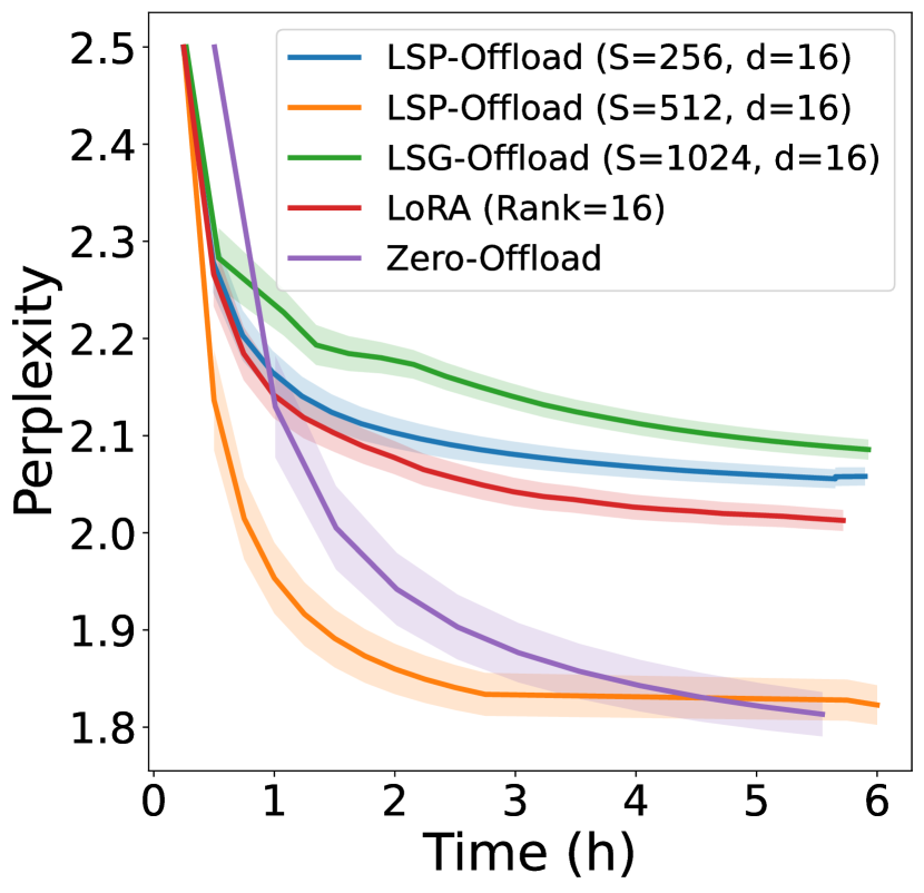
(b) Evaluation PPL. of fine-tuning the Llama-3B model w/ the workstation GPU.

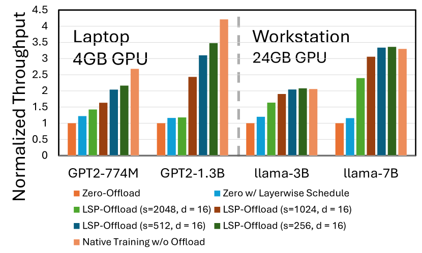
(c) Training Throughput Comparison

Figure 4: End-to-end evaluation of LSP-Offload by finetuning LLM on the Alpaca Dataset. For Fig. 4(a), Fig. 4(b), rolling average is applied for drawing the curve. The fianted area around the line shows the standard deviation.

Shown in Fig. 4(a) and Fig. 4(b), compared to Zero-Offload, LSP-Offload uses around 62.5% and 33.1% less time when converging to the same accuracy. For example, when training on the Laptop GPU, LSP-Offload achieves the evaluation perplexity of 1.82 after 2 hours of training, while reaching the same perplexity takes 4.5 hours with Zero-Offload. In terms of the training accuracy, LSP-Offload converges to the perplexity of 1.63 after 12 hours, which is achieved by Zero-Offload after 20 hours. One thing we want to mention that training all parameters as in Zero-Offload does converge to lower perplexity of 1.59. However, the training time which takes about approximately 30 hours makes the performance gain less favorable.

Moreover, compared to LoRA, LSP-Offload is able to achieve higher training accuracy. For example, LoRA converges to the perplexity of 2.15 and 2.05 in the laptop and workstation setting respectively, which are 30% and 13% higher than the final perplexity of LSP-Offload. This finding verifies the intuition that LSP-Offload can have better performance by optimizing in larger subspace.

Training Throughput Comparison.

In Fig. 4(c), we show the comparison of training throughput for different configurations. When trained on a subspace of size $512\times 512$, we are able to achieve 2.03, 3.09, 2.04, 3.33 times higher training throughput for the 4 test cases listed Fig. 4(c). Compared to the native training without offloading, LSP-Offload slows down on average 10.6%, 16.7%, 38.3% with the subspace of size 256, 512, 1024. Specifically, when trained on the workstation GPU with subspace size of smaller or equal to 512, LSP-Offload is able to obtain 2% higher throughput as compared to native training due to the fully paralleled optimizer update step on CPU. Lastly, applying the layer-wise schedule to Zero’s schedule yields on average 18% increase in the throughput.

Hyper parameters for LSP training.

We empirically compare the performance of different subspace sizes and the number of non-zero values per row in the sparse projector. While smaller subspace sizes limit the optimization space, we found too large subspace can lead to low accuracy because of over fitting. Shown in Fig. 4(b), training with subspace of size 512 outperform training with either 256 and 1024. But the training loss is 0.61 for the subspace of size 1024 and 0.72 for the subspace of size 512.

7 Limitation

While efficient, LSP-Offload introduces a few hyper parameters which may need careful selection for the best performance (Fig. 4(a), 4(b)), including the choice of the d-sparse matrix, the frequency to update the subspace, the threshold for the subspace update, etc. Moreover, the current prototype of LSP-Offload does not include the quantization technique, which is fully compatible with our approach and we leave for the future work.

8 Conclusion

In this paper, we observed that in the commodity setting, current offloading frameworks are fundamentally bottle necked by the expensive communication or the compute on CPU. Motivated by the PEFT method, we designed LSP-Offload to enable near-native speed fine-tuning by constraining the parameter update onto a subspace. Technically, we projected the gradient onto a subspace using a sparse projector, and boosted its performance by minimizing the empirical bias. Compared to the prior PEFT approaches (Galore, LORA), with the same amount of additional memory on GPU, we are able to optimize in subspace of arbitrary subspace. In evaluation, we verified that LSP training can converge at the same rate with native training on the GLUE dataset. Also, in the end-to-end comparison with SOTA offloading framework on instruction-tuning task, we are able to achieve up to 3.33x higher training throughput and converge to the same accuracy with 37.5% to 66.9% of time.

9 Appendix

Table 4: Configurations and timings for training/fine-tuning the GPT2-1.3B Model on the Nvidia A1000 Laptop GPU (4GB) and Intel Core-i7 12800H CPU (32GB). For the Update stage, we measure the fused Adam kernel with thread-level parallelism and SIMD optimizations. For the Bandwidth, we measure the PCIe bandwidth with a pinned memory buffer.

Parameters	Optimizer State	Activations	CPU-GPU Bandwidth	#Layer	GPU Memory
2.6GB	7.8GB	0.5GB	10$\sim$15GB/s	40	4GB
FWD on CPU	BWD on CPU	UPD on CPU	FWD on GPU	BWD on GPU	UPD on GPU
0.16s/layer	0.27s/layer	0.08s/layer	4.5ms/layer	8.7ms/layer	7.9ms/layer

9.1 Proof of theorem 1

Before proving Theorem 1, we listed the lemmas used in the proof.

Lemma 1 (Matrix Chernoff).

Let $M_{1},...,M_{t}$ be independent matrix valued random variables such that $M_{i}\in\mathbb{R}^{d_{1}\times d_{2}}$ and $\mathbb{E}[M_{i}]=0$. If $\|M_{i}\|_{2}\leq\gamma$ holds almost surely for all $i\in\{1,...,t\}$, then for every $\epsilon>0,0<\delta<1$, when $t>\frac{8\gamma^{2}}{3\epsilon^{2}}log(\frac{d_{1}+d_{2}}{\delta})$,

$$Pr(\|\frac{1}{t}\Sigma_{i}M_{i}\|_{2}>\epsilon)\leq\delta$$

Lemma 2.

For a subspace compressor $\mathcal{C}$, weight matrix $W\in\mathbb{R}^{m\times n}$, suppose $\|\mathcal{C}(\nabla_{W}f_{x})-\nabla_{W}f_{x}\|<\gamma$ holds for all data $x$, we can bound the bias by the empirical bias on a random sub-sampled dataset $S$ of size $\mathcal{O}(\frac{8\gamma^{2}}{3\epsilon^{2}}\log{\frac{m+n}{\delta}})$ with probability at least $1-\delta$,

$$\|\textbf{b}(W)\|_{2}:=\|\mathbb{E}_{x}[\mathcal{C}(\nabla f_{x}(W))]-\nabla f(W)\|\leq\|\mathcal{C}(\nabla f_{S}(W))-\nabla f_{S}(W)\|_{2}+\epsilon$$

Proof.

We prove by Matrix Chernoff Bound. For data $x\in S$, let $M_{x}=\mathcal{C}(\nabla f_{x}(W))-\nabla f_{x}(W)-\textbf{b}(W)$. By definition, $\mathbb{E}[M_{x}]=0$. Under Assumption 1, $\|M_{x}\|<\gamma$. Also,

$$\frac{1}{|S|}\Sigma_{x\in S}M_{x} =\frac{1}{|S|}\Sigma_{x\in S}(\mathcal{C}(\nabla f_{x}(W))-\nabla f_{x}(W)-\textbf{b}(W))$$

$$=\frac{1}{|S|}\Sigma_{x\in S}(\mathcal{C}(\nabla f_{x}(W)))-\nabla f_{S}(W)-\textbf{b}(W)$$

$$=\mathcal{C}(\frac{1}{|S|}\Sigma_{x\in S}\nabla f_{x}(W))-\nabla f_{S}(W)-\textbf{b}(W)$$

$$=\mathcal{C}(\nabla f_{S}(W))-\nabla f_{S}(W)-\textbf{b}(W)$$

. By Matrix Chernoff, we have that for $|S|>\frac{8\gamma^{2}}{3\epsilon^{2}}\log{\frac{m+n}{\delta}}$

$$Pr(\|\mathcal{C}(\nabla f_{S}(W))-\nabla f_{S}(W)-\textbf{b}(W)\|_{2}>\epsilon)\leq\delta$$

. Therefore, with probability $1-\delta$,

$$\|\textbf{b}(W)\|_{2} \leq\|\mathcal{C}(\nabla f_{S}(W))-\nabla f_{S}(W)\|_{2}+\|\mathcal{C}(\nabla f_{S}(W))-\nabla f_{S}(W)-\textbf{b}(W)\|_{2}$$

$$\leq\|\mathcal{C}(\nabla f_{S}(W))-\nabla f_{S}(W)\|_{2}+\epsilon$$

∎

Theorem 2.

[13] For any $\epsilon>0,0<\delta<1$, suppose f is a L-smooth function, and for any weight matrices $W$, $\|\textbf{b}(W)\|\leq m\nabla f(W)+\psi$, where $0<m<1,\psi>0$, and stepsize $\eta=\frac{1}{L}$, where $F:=\mathbb{E}[f(W_{0})]-f^{*}$, with probability $1-\delta$,

$$T=\mathcal{O}(\frac{1}{\epsilon})\cdot\frac{LF}{(1-m)}$$

. iterations are sufficient to obtain $\min_{t\in[T]}\mathbb{E}\|\nabla f(W_{t})\|^{2}=\mathcal{O}(\epsilon+\frac{\psi}{1-m})$

Now, we prove Theorem 1

Proof.

We analyze with some $\delta_{0}>0,\beta>0$. From lemma 2, under the Assumption 1, we know that for $|S|>\frac{8\gamma^{2}}{3\beta^{2}}\log{\frac{m+n}{\delta_{0}}}$, with probability $1-\delta_{0}$,

$$\|\textbf{b}(W)\|_{2}=\|\mathbb{E}_{x}[\mathcal{C}(\nabla f_{x}(W))]-\nabla f(W)\|\leq\|\mathcal{C}(\nabla f_{S}(W))-\nabla f_{S}(W)\|_{2}+\beta$$

Also, because $\mathbb{E}[\nabla f_{S}(W)]=\nabla f(W)$, by Matrix Chernoff Bound, under the Assumption 1, we have for $|S|>\frac{8\gamma^{2}}{3\beta^{2}}log(\frac{d_{1}+d_{2}}{\delta_{0}})$, with probability $1-\delta_{0}$,

$$\|\nabla f_{S}(W)-\nabla f(W)\|_{2}\leq\beta$$

We bound the bias for every parameter update step,

$$\|\textbf{b}(W)\|_{F} \leq c\|\textbf{b}(W)\|_{2}$$

$$\text{with prob}~{}1-\delta_{0} \leq c\|\mathcal{C}(\nabla f_{S}(W))-\nabla f_{S}(W)\|_{2}+c\beta$$

by Assumption 3 $$\leq c\alpha\|\nabla f_{S}(W)\|_{2}+c\beta$$

$$\text{with prob}~{}1-\delta_{0} \leq c\alpha\|\nabla f(W)\|_{2}+c\beta+c\alpha\beta$$

$$\leq c\alpha\|\nabla f(W)\|_{F}+c\beta+c\alpha\beta$$

Thus, with probability $1-2\delta_{0}$,

$$\|\textbf{b}(W)\|_{F}^{2}\leq 2c^{2}\alpha^{2}\|\nabla f(W)\|_{F}^{2}+2c^{2}\beta^{2}(1+\alpha)^{2}$$

, By plugging this into Thm. 2 for all steps from 1 to T, we have that for $|S|>\frac{8\gamma^{2}}{3\beta^{2}}log(\frac{d_{1}+d_{2}}{\delta_{0}})$, with probability $1-2T\delta_{0}$,

$$T=\mathcal{O}(\frac{1}{\epsilon})\cdot\frac{LF}{(1-2c^{2}\alpha^{2})}$$

iterations are sufficient to obtain $\min_{t\in[T]}\mathbb{E}\|\nabla f(W_{t})\|^{2}=\mathcal{O}(\epsilon+\frac{2c^{2}\beta^{2}(1+\alpha)^{2}}{1-2c^{2}\alpha^{2}})$. Setting $\delta_{0}=\frac{\delta}{2T}$ concludes the proof. ∎

9.2 Experiment Configurations

9.2.1 The GLUE Experiment

For the GLUE experiment, we use the batch size of 16 and set the learning rate of 1e-4 for the baseline and 1e-5 for LSP-Offload. For LSP-Offload, we update the subspace at the beginning of each epoch or every 1000 iterations. The threshold for the compression is set to be 0.3.

9.2.2 The Instruction Fine-tuning Experiment

For the instruction fine-tuning experiment, we use the batch size of 4 for the GPT2-774M model and 16 for the Llama-3B model, which is the largest without exceeding the GPU memory. The learning rate the best from $1e-4,1e-5,1e-6$, which is 1e-4 for LSP-Offload, and 1e-5 for both LoRA and Zero-Offload. For LSP-Offload, we update the subspace every 1000 iterations. The threshold for the compression is set to be 0.5.

References

- [1] Tianqi Chen, Bing Xu, Chiyuan Zhang, and Carlos Guestrin. Training deep nets with sublinear memory cost. arXiv preprint arXiv:1604.06174, 2016.
- [2] Tim Dettmers, Artidoro Pagnoni, Ari Holtzman, and Luke Zettlemoyer. Qlora: Efficient finetuning of quantized llms. Advances in Neural Information Processing Systems, 36, 2024.
- [3] Demi Guo, Alexander M Rush, and Yoon Kim. Parameter-efficient transfer learning with diff pruning. arXiv preprint arXiv:2012.07463, 2020.
- [4] Edward J Hu, Yelong Shen, Phillip Wallis, Zeyuan Allen-Zhu, Yuanzhi Li, Shean Wang, Lu Wang, and Weizhu Chen. Lora: Low-rank adaptation of large language models. arXiv preprint arXiv:2106.09685, 2021.
- [5] Chien-Chin Huang, Gu Jin, and Jinyang Li. Swapadvisor: Pushing deep learning beyond the gpu memory limit via smart swapping. In Proceedings of the Twenty-Fifth International Conference on Architectural Support for Programming Languages and Operating Systems, pages 1341–1355, 2020.
- [6] Daniel M Kane and Jelani Nelson. Sparser johnson-lindenstrauss transforms. Journal of the ACM (JACM), 61(1):1–23, 2014.
- [7] Diederik P Kingma and Jimmy Ba. Adam: A method for stochastic optimization. arXiv preprint arXiv:1412.6980, 2014.
- [8] Vladislav Lialin, Sherin Muckatira, Namrata Shivagunde, and Anna Rumshisky. Relora: High-rank training through low-rank updates. In Workshop on Advancing Neural Network Training: Computational Efficiency, Scalability, and Resource Optimization (WANT@ NeurIPS 2023), 2023.
- [9] Yinhan Liu, Myle Ott, Naman Goyal, Jingfei Du, Mandar Joshi, Danqi Chen, Omer Levy, Mike Lewis, Luke Zettlemoyer, and Veselin Stoyanov. Roberta: A robustly optimized bert pretraining approach. arXiv preprint arXiv:1907.11692, 2019.
- [10] Samyam Rajbhandari, Jeff Rasley, Olatunji Ruwase, and Yuxiong He. Zero: Memory optimizations toward training trillion parameter models. In SC20: International Conference for High Performance Computing, Networking, Storage and Analysis, pages 1–16. IEEE, 2020.
- [11] Samyam Rajbhandari, Olatunji Ruwase, Jeff Rasley, Shaden Smith, and Yuxiong He. Zero-infinity: Breaking the gpu memory wall for extreme scale deep learning. In Proceedings of the International Conference for High Performance Computing, Networking, Storage and Analysis, pages 1–14, 2021.
- [12] Jie Ren, Samyam Rajbhandari, Reza Yazdani Aminabadi, Olatunji Ruwase, Shuangyan Yang, Minjia Zhang, Dong Li, and Yuxiong He. ZeRO-Offload: Democratizing Billion-Scale model training. In 2021 USENIX Annual Technical Conference (USENIX ATC 21), pages 551–564, 2021.
- [13] Ahmad Ajalloeian1 Sebastian U Stich. Analysis of sgd with biased gradient estimators. arXiv preprint arXiv:2008.00051, 2020.
- [14] Rohan Taori, Ishaan Gulrajani, Tianyi Zhang, Yann Dubois, Xuechen Li, Carlos Guestrin, Percy Liang, and Tatsunori B. Hashimoto. Stanford alpaca: An instruction-following llama model. https://github.com/tatsu-lab/stanford_alpaca, 2023.
- [15] Mojtaba Valipour, Mehdi Rezagholizadeh, Ivan Kobyzev, and Ali Ghodsi. Dylora: Parameter efficient tuning of pre-trained models using dynamic search-free low-rank adaptation. arXiv preprint arXiv:2210.07558, 2022.
- [16] Alex Wang, Amanpreet Singh, Julian Michael, Felix Hill, Omer Levy, and Samuel R Bowman. Glue: A multi-task benchmark and analysis platform for natural language understanding. arXiv preprint arXiv:1804.07461, 2018.
- [17] Haoyang Zhang, Yirui Eric Zhou, Yuqi Xue, Yiqi Liu, and Jian Huang. G10: Enabling an efficient unified gpu memory and storage architecture with smart tensor migrations. arXiv preprint arXiv:2310.09443, 2023.
- [18] Jiawei Zhao, Zhenyu Zhang, Beidi Chen, Zhangyang Wang, Anima Anandkumar, and Yuandong Tian. Galore: Memory-efficient llm training by gradient low-rank projection. arXiv preprint arXiv:2403.03507, 2024.