Finite temperature detection of quantum critical points: a comparative study

Abstract

We comparatively study three of the most useful quantum information tools to detect quantum critical points (QCPs) when only finite temperature data are available. We investigate quantitatively how the quantum discord, the quantum teleportation based QCP detectors, and the quantum coherence spectrum pinpoint the QCPs of several spin-$1/2$ chains. We work in the thermodynamic limit (infinite number of spins) and with the spin chains in equilibrium with a thermal reservoir at temperature $T$. The models here studied are the $XXZ$ model with and without an external longitudinal magnetic field, the Ising transverse model, and the $XY$ model subjected to an external transverse magnetic field.

I Introduction

The use of quantum information based tools to characterize a quantum phase transition (QPT) brought to light the existence of genuine quantum correlations during a QPT ost02 ; osb02 ; wu04 ; ver04 ; oli06 ; dil08 ; sar08 ; fan14 ; gir14 ; hot08 ; hot09 ; ike23a ; ike23b ; ike23c ; ike23d . A QPT is characterized by a drastic change in the ground state describing a macroscopic system while we modify the system’s Hamiltonian sac99 ; gre02 ; gan10 ; row10 . Traditionally, to properly observe a QPT, we need to reduce the system’s temperature such that the thermal fluctuations become small enough to not excite the system away from its ground state. In this scenario the system can be considered for all practical purposes at the absolute zero temperature ($T=0$) and we can be reassured that all measurements give information about the system’s ground state alone.

When the temperature $T$ is high enough, the probability to find the system in one of its excited states is no longer negligible. In this case the analysis of a QPT, a genuine feature of the system’s ground state, is more subtle. Some tools may not work at all, furnishing no clue to the existence of a quantum critical point (QCP) for the ground state. For instance, the entanglement of formation woo98 between two spins is zero for some models in the vicinity of the QCP if the system is above a certain temperature wer10 ; wer10b .

Fortunately, there are quantum information tools that still allow us to infer the correct location of a QCP when only finite $T$ data are at hand. Our main goal here is to comparatively study the efficacy of the most promising tools to detect QCPs with finite $T$ data. Specifically, we will study the three tools that stand out in this scenario, namely, the thermal quantum discord wer10b , the quantum coherence spectrum li20 , and the teleportation based QCP detectors pav23 ; pav24 . The first tool is the quantum discord (QD) oll01 ; hen01 computed for systems in thermal equilibrium wer10 , the second tool is a spin-off of the quantum coherence (QC) wig63 ; fan14 ; gir14 , and the third one is based on the quantum teleportation protocol ben93 ; yeo02 ; rig17 .

It is worth mentioning that the comparison among the tools described above does not take into account their computational complexity. Furthermore, we do not take into account their operational meaning and experimental feasibility either.

Indeed, the computation of the QD is not an easy task and for high spins it is extremely difficult mal16 . The reason for that is related to how the computational resources needed to its evaluation scale as we increase the size of the system under investigation (QD is an NP-complete problem hua14 ). Also, QD does not have a direct experimental meaning and so far no general method to its direct measurement is available. A similar analysis applies to the spectrum of the QC li20 . Its computation is also resource intensive and no direct way for measuring it is available pav23 . The third set of tools, namely, the quantum teleportation based QCP detectors, does not suffer from those problems, having a direct experimental meaning and being amenable to theoretical analysis for high spin systems pav23 ; pav24 .

II The critical point detectors

The key ingredient needed to theoretically compute the following quantum information based QCP detectors is a two-qubit density matrix. This density matrix completely characterizes a pair of nearest neighbor spins within the spin chain and it is obtained by tracing out all but these two spins from the canonical ensemble density matrix describing the whole chain. In Sec. III we will come back to this point providing further details. However, the important point now is that for all the models investigated in this work, this two-qubit density matrix has the following form wer10b ; pav23 ; pav24 ; osb02 ,

$$\rho_{23}=\left(\begin{array}[]{cccc}a&0&0&e\\ 0&b&c&0\\ 0&c&b&0\\ e&0&0&d\\ \end{array}\right),$$ (1)

where $a,b,c,d,e$ are real numbers. The values of these numbers depend on the particular model and on the temperature of the heat bath. In Eq. (1), the subscripts $2$ and $3$ denote any two nearest neighbor spins while we reserve the number $1$ to represent an extra qubit from or outside the spin chain that is teleported from Alice (qubit $2$) to Bob (qubit $3$) [see Sec. II.3].

II.1 Thermal quantum discord

The QD aims to capture all genuine quantum correlations between two physical systems (a bipartite system). It is defined as the difference between two non-equivalent ways of extending to the quantum realm the classical mutual information between a bipartite system oll01 ; hen01 . For the density matrix (1), the QD is cil10 ; hua13 ; yur15

$$\mathcal{QD}=S(\rho_{3})-S(\rho_{23})+\min_{\theta\in[0,\frac{\pi}{2}]}\tilde{S}(\theta),$$ (2)

where $\rho_{3}=\mbox{Tr}_{2}{\rho_{23}}$ is the reduced state describing qubit $3$, obtained after tracing out qubit $2$ from $\rho_{23}$, $S(\rho_{3})$ and $S(\rho_{23})$ are, respectively, the von Neumann entropy of the states $\rho_{3}$ and $\rho_{23}$,

$$S(\rho_{3})\! \!=\! \!-(a+b)\ln(a+b)-(b+d)\ln(b+d),$$ (3)

$$S(\rho_{23})\! \!=\! \!-\frac{a+d-\sqrt{(a-d)^{2}+4e^{2}}}{2}$$ (4)

$$\times\ln\left(\frac{a+d-\sqrt{(a-d)^{2}+4e^{2}}}{2}\right)$$

$$-\frac{a+d+\sqrt{(a-d)^{2}+4e^{2}}}{2}$$

$$\times\ln\left(\frac{a+d+\sqrt{(a-d)^{2}+4e^{2}}}{2}\right)$$

$$-\!\left(b-c\right)\ln\!\left(b-c\right)\!-\!\left(b+c\right)\ln\!\left(b+c\right)\!,$$

and

$$\tilde{S}(\theta)=\Lambda_{1}\ln\Lambda_{1}+\Lambda_{2}\ln\Lambda_{2}-\sum_{j=1}^{4}\lambda_{j}\ln\lambda_{j}.$$ (5)

In Eq. (5) we have

$$\Lambda_{1,2}\! \!=\! \!\frac{1}{2}[1\pm(a-d)\cos\theta],$$ (6)

$$\lambda_{1,2}\! \!=\! \!\frac{1}{4}(1+(a-d)\cos\theta$$

$$\!\pm\!\! \!\!\left.\sqrt{\![a-d+(\!a-2b+d)\cos\theta]^{2}\!+\!4(|c|+|e|)^{2}\sin^{2}\!\theta}\right)\!\!,$$

$$\lambda_{3,4}\! \!=\! \!\frac{1}{4}(1-(a-d)\cos\theta$$

$$\!\pm\!\! \!\!\left.\sqrt{\![a-d-(\!a-2b+d)\cos\theta]^{2}\!+\!4(|c|+|e|)^{2}\sin^{2}\!\theta}\right)\!\!.$$

Note that in the previous expressions “$\ln$” is the natural logarithm and the minimization of $\tilde{S}(\theta)$ must be implemented numerically. Once we have the two-qubit density matrix as given by Eq. (1), we compute Eq. (5) and numerically search for its minimum value assuming it is a function of $\theta$, with $\theta\in[0,\pi/2]$.

II.2 Quantum coherence spectrum

The QC spectrum li20 is actually two different quantities defined to investigate the spectrum of the operator defining the QC fan14 ; gir14 . The QC studied here gir14 is a simplified version of the Wigner-Yanase skew information wig63 , which aims at quantifying the amount of information a density matrix contains with respect to an observable, in particular when the latter does not commute with the density matrix. Note that by its very definition, the QC is observable dependent. QC is also related to an interesting extension of the Heisenberg uncertainty relation for mixed states luo05 or to the quantification of the coherence of a quantum state gir14 .

In its more experimentally friendly version and for a two-qubit density matrix, QC is defined as gir14 ,

$$\mathcal{QC}(K)=-\frac{1}{4}\mbox{Tr}\{[\rho_{23},K]^{2}\},$$ (9)

where Tr denotes the trace operation, $[A,B]=AB-BA$, and $K$ is a $4\times 4$ matrix representing any observable associated with a two-qubit system. Note that we are highlighting in the definition above the dependence of QC on the observable $K$.

If one computes the spectrum of $[\rho_{23},K]^{2}$, namely, determines its four eigenvalues $\alpha_{1},\ldots,\alpha_{4}$, one can define the following two quantities li20 ,

$$\mathcal{S}_{QC}^{K} = -\sum_{n=1}^{4}|\alpha_{n}|\ln|\alpha_{n}|,$$ (10)

$$\mathcal{L}_{QC}^{K} = -\sum_{n=1}^{4}\ln|\alpha_{n}|.$$ (11)

The superscripts in Eqs. (10) and (11) remind us that they both depend on the observable $K$. The first quantity, $\mathcal{S}_{QC}^{K}$, is called coherence entropy and the second one, $\mathcal{L}_{QC}^{K}$, logarithm of the spectrum li20 . We should also note that in Ref. li20 the above quantities were defined without taking the moduli of the eigenvalues. This is inconsistent since, as we will show next, these eigenvalues can become negative for certain observables if we use the density matrix (1). In other words, we must take the absolute value of $\alpha_{n}$, as in Eqs. (10) and (11), if we want the logarithm to be a well defined real function. Furthermore, the second quantity above, $\mathcal{L}_{QC}^{K}$, even when defined with $|\alpha_{n}|$ instead of $\alpha_{n}$, continues to be ill-defined and problematic. The reason for that is related to the fact that there are certain combinations of $\rho_{23}$ and $K$ that lead to at least one $\alpha_{n}$ being zero. And if $\alpha_{n}$ is zero $\ln|\alpha_{n}|$ is not defined ($\lim_{x\rightarrow 0}\ln|x|\rightarrow-\infty$). On the other hand, $\mathcal{S}_{QC}^{K}$ is perfectly legitimate since $\lim_{x\rightarrow 0}|x|\ln|x|=0$. For a clear and simple illustration of this point, see the discussion around Eq. (19).

We will provide in Sec. III a couple of examples where at least one $\alpha_{n}$ is zero. It will turn out that the “robustness” of $\mathcal{L}_{QC}^{K}$ to detect QCPs using extremely high $T$ data, as reported in Ref. li20 , is a consequence of its faulty definition. This alleged high temperature robustness is not even restricted to the QCPs either. In many cases $\alpha_{n}$ is zero in regions of the parameter space defining the Hamiltonian where no QPT is taking place. Also, whenever $\alpha_{n}$ becomes zero, at or away from a QCP, this feature is independent of the value of the system’s temperature and is a consequence of a particular symmetry of the system’s Hamiltonian. This is the case for all the models investigated in ref. li20 and where $\mathcal{L}_{QC}^{K}$ was shown to be insensitive to temperature increases (see Sec. III).

Following Ref. li20 , we restrict our analysis to three local observables $K$, namely, $K=\mathbb{1}\otimes\sigma^{x},\mathbb{1}\otimes\sigma^{y}$, and $\mathbb{1}\otimes\sigma^{z}$, where $\mathbb{1}$ is the $2\times 2$ identity matrix acting on qubit 2 (Alice) and $\sigma^{x},\sigma^{y}$, and $\sigma^{z}$ are the standard Pauli matrices acting on qubit 3 (Bob). The matrix representation of the two-qubit state $\rho_{23}$ [see Eq. (1)] is given in the computational basis $\{|00\rangle,|01\rangle,|10\rangle,|11\rangle\}$, where $\sigma^{z}$ is diagonal.

A direct calculation using Eq. (1) and the representation of $\mathbb{1}\otimes\sigma^{x}$ in the basis where $\sigma^{z}$ is diagonal leads to the following eigenvalues for $[\rho_{23},\mathbb{1}\otimes\sigma^{x}]^{2}$,

$$\alpha_{1,2}^{x} = \alpha(1,1),$$ (12)

$$\alpha_{3,4}^{x} = \alpha(-1,1),$$ (13)

where

$$\alpha(\epsilon_{1},\epsilon_{2}) = -\frac{1}{2}\left[(a-b)^{2}+(b-d)^{2}+2(c-\epsilon_{2}e)^{2}\right.$$ (14)

$$+\left.\epsilon_{1}(a-2b+d)\sqrt{(a-d)^{2}+4(c-\epsilon_{2}e)^{2}}\right].$$

Similarly, for $[\rho_{23},\mathbb{1}\otimes\sigma^{y}]^{2}$ we have

$$\alpha_{1,2}^{y} = \alpha(1,-1),$$ (15)

$$\alpha_{3,4}^{y} = \alpha(-1,-1),$$ (16)

and for $[\rho_{23},\mathbb{1}\otimes\sigma^{z}]^{2}$ we get

$$\alpha_{1,2}^{z} = -4c^{2},$$ (17)

$$\alpha_{3,4}^{z} = -4e^{2}.$$ (18)

Note that the superscripts in the eigenvalues above mark the corresponding operator $K$ that we used in each one of the three previous calculations. Also, all eigenvalues are doubly degenerate.

If we look at the eigenvalues given by Eqs. (17) and (18), we clearly see that they are all negative. This proves that we must define Eqs. (10) and (11) using the magnitude of those eigenvalues. We should not use the eigenvalues directly, as was done in Ref. li20 . In Eqs. (12) and (13) or in Eqs. (15) and (16) we also have that at least two out of four eigenvalues are clearly negative. This is true because a pair of degenerate eigenvalues is given by either $-u+v$ or $-u-v$, with $u$ and $v$ positive numbers. And whenever $v<u$ all four eigenvalues become negative.

Before we move on, we show a very simple case where we have two out of four eigenvalues zero. This happens for all the operators $K$ that we use here, proving that $\mathcal{L}_{QC}^{K}$, Eq. (11), cannot be defined for all two-qubit states.

Let us take the following Bell state, namely, $|\Phi^{+}\rangle=(|00\rangle+|11\rangle)/\sqrt{2}$. Its density matrix is

$$\rho_{\Phi^{+}}=|\Phi^{+}\rangle\langle\Phi^{+}|=\left(\begin{array}[]{cccc}\frac{1}{2}&0&0&\frac{1}{2}\\ 0&0&0&0\\ 0&0&0&0\\ \frac{1}{2}&0&0&\frac{1}{2}\end{array}\right).$$ (19)

Comparing with Eq. (1), we get $a=d=e=1/2$ and $b=c=0$. Therefore, Eqs. (12)-(18) become

$$\alpha_{1,2}^{x}=\alpha_{1,2}^{y}=\alpha_{3,4}^{z} = -1,$$ (20)

$$\alpha_{3,4}^{x}=\alpha_{3,4}^{y}=\alpha_{1,2}^{z} = 0.$$ (21)

The above result is not restricted to this particular Bell state. The same is true for the other three. Moreover, the existence of null eigenvalues is not an exclusive feature of an entangled state, such as the Bell state above. If we employ, for instance, the separable states $|00\rangle$ or $|11\rangle$, we also get a pair of null eigenvalues.

II.3 Teleportation based QCP detectors

The teleportation based QCP detectors pav23 ; pav24 use a pair of qubits ($\rho_{23}$) from a spin chain as the quantum resource (quantum communication channel) through which the standard teleportation protocol ben93 is implemented. Since a QPT induces a drastic change in the system’s ground state, it is expected that the state describing this pair of qubits also changes substantially. This change will eventually affect the efficiency of the teleportation protocol. As such, an abrupt change in the efficiency of the teleportation protocol may indicate a QPT and the exact location of the corresponding QCP pav23 ; pav24 .

In general, the state describing a pair of qubits from a spin chain is a mixed state. Thus, to properly construct the teleportation based QCP detectors, we need to recast the standard teleportation protocol in the formalism of density matrices pav23 ; pav24 ; rig17 ; rig15 .

Qubits $2$ and $3$, described by $\rho_{23}$, constitute the quantum resource shared by Alice (qubit $2$) and Bob (qubit $3$). It is obtained tracing out from the whole chain all but these two qubits. The qubit to be teleported or input qubit can be an external qubit from the chain pav23 or another qubit from the spin chain pav24 . In both cases it is formally described by the density matrix $\rho_{1}$. If the input qubit does not belong to the chain, we have the external teleportation based QCP detector while if the input belongs to the chain we have the internal teleportation based QCP detector. In Figs. 1 and 2 we schematically show how the two approaches work.

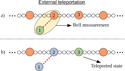
Figure 1: (color online) A single run of the external teleportation protocol using a pair of qubits from a spin chain is described by the following steps. Alice and Bob agree on which pair of qubits to use as the quantum resource to implement the teleportation protocol. This pair is illustrated by qubits $2$ and $3$ in the figure. Alice brings an external qubit to be teleported to Bob. This is qubit $1$ depicted in the figure. Subsequently Alice projects qubits $1$ and $2$ onto a Bell state. This is a standard Bell measurement (BM). See panel (a) above. Alice then tells Bob of her BM result by sending two classical bits to Bob since there are four possible outcomes after a BM. Finally, based on the information received by Bob from Alice, he implements a corresponding unitary operation on his qubit to finish the protocol. This step is represented in the panel (b) above.

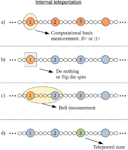
Figure 2: (color online) A single run of the internal teleportation protocol using a pair of qubits from a spin chain is described by the following steps. Alice projects the qubit $1$ onto the computational basis [panel (a)]. Then, she either applies onto it the spin flip operation ($\sigma_{1}^{x}$) or does nothing [panel (b)] according to recipe given in Ref. pav24 . Finally, Alice and Bob execute the standard teleportation protocol as explained in Fig. 1 [panels (c) and (d)].

For the external teleportation protocol, the density matrix describing the three qubits before the teleportation begins is pav23

$$\rho=\rho_{1}\otimes\rho_{23},$$ (22)

where $\rho_{1}$ is an arbitrary pure state that Alice can freely choose and $\rho_{23}$ is the density matrix describing a pair of qubits from the spin chain. For the internal teleportation protocol, the state describing the three qubits is in general given by $\rho_{123}$ pav24 , where the latter is obtained by tracing out all but qubits $1,2$, and $3$ from the state describing the whole chain. In order to effectively obtain Eq. (22) in the internal teleportation protocol, Alice has to implement steps (a) and (b) described in Fig. 2 before starting the teleportation protocol. See ref. pav24 for all the details of how this can be accomplished. At the end, Alice and Bob will share an ensemble of states effectively given by Eq. (22), where $\rho_{23}$ is the density matrix describing a pair of qubits from the spin chain and $\rho_{1}$ is the density matrix associated with a single spin from the chain.

At the end of one run of the teleportation protocol, as described in Figs. 1 and 2, qubit $3$ with Bob is pav23 ; pav24 ; rig17

$$\rho_{{}_{B_{j}}}=\frac{U_{j}Tr_{12}[P_{j}\rho P_{j}]U_{j}^{\dagger}}{Q_{j}}.$$ (23)

In Eq. (23), $U_{j}$ is the unitary operation that Bob applies on his spin after being informed from Alice which Bell state $j$ she measured. The Bell measurement (BM) implemented by Alice projects qubits $1$ and $2$ onto one of the four Bell states. Also, $Tr_{12}$ denotes the partial trace over Alice’s spins (qubits 1 and 2) and $P_{j}$ is one of the four projectors related to a BM,

$$P_{\Psi^{\pm}} = |\Psi^{\pm}\rangle\langle\Psi^{\pm}|,$$ (24)

$$P_{\Phi^{\pm}} = |\Phi^{\pm}\rangle\langle\Psi^{\pm}|.$$ (25)

The Bell states are given by

$$|\Psi^{\pm}\rangle = (|01\rangle\pm|10\rangle)/\sqrt{2},$$ (26)

$$|\Phi^{\pm}\rangle = (|00\rangle\pm|11\rangle)/\sqrt{2}.$$ (27)

The denominator in Eq. (23) gives the probability of Alice measuring the Bell state $j$ pav23 ; rig17 ,

$$Q_{j}=Tr[{P_{j}\rho}].$$ (28)

We should note that the unitary operation $U_{j}$ that Bob applies on his qubit also depends on the type of quantum resource shared with Alice pav23 ; pav24 ; rig17 . In the standard teleportation protocol, where the state $\rho_{23}$ is a Bell state $|k\rangle$, with $k=\Psi^{\pm},\Phi^{\pm}$, we have that $U_{j}$ is given by the following set $S_{k}$ of four unitary operators,

$$S_{\Phi^{+}}=\{U_{\Phi^{+}},U_{\Phi^{-}},U_{\Psi^{+}},U_{\Psi^{-}}\}=\{\mathbb{1},\sigma^{z},\sigma^{x},\sigma^{z}\sigma^{x}\},$$ (29)

$$S_{\Phi^{-}}=\{U_{\Phi^{+}},U_{\Phi^{-}},U_{\Psi^{+}},U_{\Psi^{-}}\}=\{\sigma^{z},\mathbb{1},\sigma^{z}\sigma^{x},\sigma^{x}\},$$ (30)

$$S_{\Psi^{+}}=\{U_{\Phi^{+}},U_{\Phi^{-}},U_{\Psi^{+}},U_{\Psi^{-}}\}=\{\sigma^{x},\sigma^{z}\sigma^{x},\mathbb{1},\sigma^{z}\},$$ (31)

$$S_{\Psi^{-}}=\{U_{\Phi^{+}},U_{\Phi^{-}},U_{\Psi^{+}},U_{\Psi^{-}}\}=\{\sigma^{z}\sigma^{x},\sigma^{x},\sigma^{z},\mathbb{1}\}.$$ (32)

Here, the state $\rho_{23}$ is a mixed state that changes after a QPT. In one phase it is closer to one Bell state and in another phase it is more similar to another one. Therefore, the teleportation based QCP detectors are defined by picking the optimal case out of the four sets $S_{k}$ above.

For the external teleportation based QCP detector, the fidelity uhl76 ; nie00 is employed to assess the efficiency of the teleportation protocol. The fidelity quantifies how close or similar two states are to each other. It is employed here to compare the similarity of the output state with Bob at the end of the protocol with the input state teleported by Alice. Since Alice always choose pure states to teleport to Bob, the fidelity becomes

$$F_{j}(|\psi\rangle,S_{k})=\langle\psi|\rho_{{}_{B_{j}}}|\psi\rangle,$$ (33)

where $|\psi\rangle$ is any single qubit pure state external to the chain (see Fig. 1) while $\rho_{{}_{B_{j}}}$ is given by Eq. (23). The fidelity is one if the two states are identical and zero if they are orthogonal.

After several runs of the protocol, each Bell state will be measured by Alice with probability $Q_{j}$. Thus, the relevant quantity in this case is the average fidelity pav23 ; gor06 ,

$$\overline{F}(|\psi\rangle,S_{k})=\sum_{j=\Psi^{\mp},\Phi^{\mp}}Q_{j}F_{j}(|\psi\rangle,S_{k}).$$ (34)

Optimizing over $|\psi\rangle$ (picking the maximum over all pure input states on the Bloch sphere) and over $S_{k}$ (the four sets of unitary corrections available to Bob), we get the maximum mean fidelity pav23 ,

$$\overline{\mathcal{F}}=\max_{\{|\psi\rangle,S_{k}\}}{\overline{F}(|\psi\rangle,S_{k})}.$$ (35)

Equation (35) is the most accurate QCP detector based on the external teleportation protocol. For the density matrix $\rho_{23}$ given by Eq. (1) we obtain

$$\overline{\mathcal{F}}_{ext}=\max\left[2b,1-2b,\frac{1}{2}+|c|+|e|\right],$$ (36)

where we used the normalization condition $\mbox{Tr}(\rho_{23})=a+2b+d=1$ to arrive at the expression above. Note that we append the subscript “ext” to $\overline{\mathcal{F}}$ to make it clear that this particular expression only applies to the external teleportation case.

We should note that $\overline{\mathcal{F}}_{ext}$ depends only on the two-qubit state $\rho_{23}$, similarly to $\mathcal{QD}$, $\mathcal{S}^{K}_{QC}$, and $\mathcal{L}^{K}_{QC}$. This means that once $\rho_{23}$ is measured or calculated, all these QCP detectors can be computed. From an experimental point of view, however, $\overline{\mathcal{F}}_{ext}$ has a clear direct operational meaning. If we teleport a representative sample of pure qubits spanning the Bloch sphere, with Bob choosing randomly the set $S_{k}$ from which he picks the unitary correction to apply on his qubit, and then compute the corresponding mean fidelities, we have that $\overline{\mathcal{F}}_{ext}$ is given by the greatest mean fidelity of all cases. The fidelity can be determined with the knowledge of Alice’s input state and Bob’s output state at the end of the teleportation protocol. Alice’s state is chosen by her and is readily known after she prepares it. Bob’s state can be experimentally determined after the teleportation is finished. Furthermore, the experimental determination of Bob’s state, a single qubit state, is accomplished by measuring one-point correlation functions (magnetization) alone pav23 ; pav24 ; nie00 . On the other hand, $\rho_{23}$ is determined by measuring two-point correlation functions pav23 ; pav24 ; nie00 .

For the internal teleportation based QCP detector, the input state and the output state are mixed states and the fidelity becomes a really complicated expression pav24 . Therefore, we use the trace distance nie00 ; tos23 ; tos24 to quantify the similarity of the input and output states. In Ref. pav24 we also showed that in this case not only the trace distance is simpler but more sensitive to detect QCPs for all the models studied here.

Alice’s input state now is fixed and given by a single spin of the chain. Since we are dealing with translational invariant spin chains,

$$\rho_{1}=\rho_{2}=\mbox{Tr}_{3}(\rho_{23})=\left(\begin{array}[]{cc}a+b&0\\ 0&b+d\end{array}\right).$$ (37)

The trace distance between Bob’s final state and Alice’s input after a single run of the teleportation protocol is pav24

$$D_{j}(S_{k})=D(\rho_{1},\rho_{{}_{B_{j}}})=\frac{1}{2}\mbox{Tr}\left|\rho_{1}-\rho_{{}_{B_{j}}}\right|,$$ (38)

where $\rho_{{}_{B_{j}}}$ and $\rho_{1}$ are given by Eqs. (23) and (37) and $|A|=\sqrt{A^{\dagger}A}$.

The trace distance is half the Euclidean distance between the points on the Bloch sphere representing the two states above. This means that two identical states have $D_{j}=0$ and orthogonal pure states have $D_{j}=1$, the maximum value for $D_{j}$. For two single qubits we have nie00

$$D_{j}(S_{k})=\frac{1}{2}\sqrt{(\Delta r_{x})^{2}+(\Delta r_{y})^{2}+(\Delta r_{z})^{2}},$$ (39)

where $\Delta r_{\alpha}(t)=\mbox{Tr}(\rho_{1}\sigma^{\alpha})-\mbox{Tr}(\rho_{{}_{B_{j}}}\sigma^{\alpha})$.

Similarly to the fidelity, the mean trace distance after several runs of the teleportation protocol is

$$\overline{D}(S_{k})=\sum_{j=\Psi^{\mp},\Phi^{\mp}}Q_{j}D_{j}(S_{k}).$$ (40)

Since the more similar two states, the lower their trace distance, we now want the minimum over all sets $S_{k}$. As such, the internal teleportation QCP detector is pav24

$$\overline{\mathcal{D}}_{int}=\min_{\{S_{k}\}}{\overline{D}(S_{k})}=|1-2(b+d)|\min\left[1-D_{-},D_{+}\right],$$ (41)

where

$$D_{\pm}=2b+d-(b+d)^{2}\pm|(b+d)^{2}-d|.$$ (42)

To arrive at Eq. (41) we employed several properties of the density matrix $\rho_{23}$. We used that $0\leq a,b,d\leq 1$, that $c$ and $e$ are real numbers, and the normalization condition $a+2b+d=1$.

The experimental procedure to directly determine the minimum mean trace distance is akin to the one already given for the maximum mean fidelity. Now, however, we do not even need to cover the whole Bloch sphere since the input state is always one spin of the chain, described by the same state $\rho_{1}$ at every run of the teleportation protocol. The experimental procedure to determine $\rho_{1}$ before the teleportation begins and Bob’s state at the end of one run of the protocol is based on the experimental determination of one-point correlation functions, as already explained when we discussed the operational interpretation of the maximum mean fidelity pav23 ; pav24 . With $\rho_{1}$, measured only once, and with Bob’s final state, measured as already described after each run of the internal teleportation protocol, all relevant quantities to the determination of the minimum mean trace distance can be computed.

III The models

The models investigated here are the local ones given in Ref. li20 , in particular those for which $\mathcal{L}^{K}_{QC}$ apparently beat the quantum discord in providing the exact location of the QCPs at finite $T$. We will be dealing with one dimensional translational invariant spin-1/2 chains in the thermodynamic limit, i.e., with $L\rightarrow\infty$, where $L$ represents the number of spins in the chain. They all satisfy periodic boundary conditions, namely, $\sigma^{x,y,z}_{L+1}=\sigma^{x,y,z}_{1}$. The subscripts in the Pauli matrices indicate on which qubit they act and the spin chains are initially in equilibrium with a thermal reservoir at temperature $T$ (heat bath).

The density matrix describing the chain of $L$ spins is the canonical ensemble density matrix,

$$\varrho=\frac{e^{-H/kT}}{Z},$$ (43)

where $Z=Tr[e^{-H/kT}]$ is the partition function and the Boltzmann’s constant is given by $k$.

If we trace out all but two nearest neighbor spins from the chain, the density matrix describing them is given by Eq. (1). In terms of the one- and two-point correlation functions, we obtain wer10b ; pav23 ; osb02

$$a = \frac{1+2\left\langle\sigma^{z}_{2}\right\rangle+\left\langle\sigma_{2}^{z}\sigma_{3}^{z}\right\rangle}{4},$$ (44)

$$b = \frac{1-\left\langle\sigma_{2}^{z}\sigma_{3}^{z}\right\rangle}{4},$$ (45)

$$c = \frac{\left\langle\sigma_{2}^{x}\sigma_{3}^{x}\right\rangle+\left\langle\sigma_{2}^{y}\sigma_{3}^{y}\right\rangle}{4},$$ (46)

$$d = \frac{1-2\left\langle\sigma^{z}_{2}\right\rangle+\left\langle\sigma_{2}^{z}\sigma_{3}^{z}\right\rangle}{4},$$ (47)

$$e = \frac{\left\langle\sigma_{2}^{x}\sigma_{3}^{x}\right\rangle-\left\langle\sigma_{2}^{y}\sigma_{3}^{y}\right\rangle}{4},$$ (48)

where for $s=x,y,z$ we have

$$z = \left\langle\sigma_{j}^{z}\right\rangle=Tr[\sigma_{j}^{z}\,\varrho],$$ (49)

$$ss = \left\langle\sigma_{j}^{s}\sigma_{j+1}^{s}\right\rangle=Tr[\sigma_{j}^{s}\sigma_{j+1}^{s}\,\varrho].$$ (50)

The details of those calculations in the thermodynamic limit ($L\rightarrow\infty$) are in Refs. yan66 ; clo66 ; klu92 ; bor05 ; boo08 ; tri10 ; tak99 ; lie61 ; bar70 ; bar71 ; pfe70 ; zho10 and in Ref. wer10b we review them in the present notation. In Ref. pav23 we also investigate how $\left\langle\sigma_{j}^{z}\right\rangle$ and $\left\langle\sigma_{j}^{s}\sigma_{j+1}^{s}\right\rangle$ behave for several values of $T$ as we drive the system’s Hamiltonian through its parameter space.

For the external teleportation based QCP detector, the density matrix describing Alice’s input is $\rho_{1}^{ext}=|\psi\rangle\langle\psi|$, where $|\psi\rangle=\cos(\theta/2)|0\rangle+\sin(\theta/2)e^{i\chi}|0\rangle$, with $\theta\in[0,\pi]$ and $\chi\in[0,2\pi)$. Maximizing the mean fidelity (34) over $S_{k}$ and over all states on the Bloch sphere, i.e., maximizing over $\theta$ and $\chi$, gives the maximal mean fidelity $\overline{\mathcal{F}}_{ext}$ [Eq. (36)]. On the other hand, Alice’s input for the internal teleportation based QCP detector is fixed by Eq. (37). In this case, we only minimize the mean trace distance (40) over $S_{k}$ to obtain the minimal mean trace distance $\overline{\mathcal{D}}_{int}$ [Eq. (41)].

If we use Eqs. (44)-(48), Eq. (36) becomes

$$\overline{\mathcal{F}}_{ext}=\max{\left[\frac{1+|xx|}{2},\frac{1+|yy|}{2},\frac{1+|zz|}{2}\right]}.$$ (51)

To obtain Eq. (51), we used the following mathematical identity, $\max[|c|+|e|]=\max[|c+e|,|c-e|]$.

Similarly, using Eqs. (44)-(48) we can write Eq. (41) as follows,

$$\overline{\mathcal{D}}_{int}=\frac{1}{4}\left[(2-|z^{2}+zz|)|z|+|z^{3}-z\cdot zz|\right],$$ (52)

where the dot between $z$ and $zz$ means the standard multiplication between two real numbers.

We should note that Eq. (52) is not useful to analyze QPTs for spin chains with zero magnetization pav24 . Looking at Eq. (52), we easily see that whenever $z=0$ we always have $\overline{\mathcal{D}}_{int}=0$. This is why $\overline{\mathcal{D}}_{int}$ does not show up when we study the first case below.

III.1 The XXZ model with no field

The Hamiltonian ($\hbar=1$) describing the XXZ model with no external magnetic field is

$$H=\sum_{j=1}^{L}\left(\sigma^{x}_{j}\sigma^{x}_{j+1}+\sigma^{y}_{j}\sigma^{y}_{j+1}+\Delta\sigma^{z}_{j}\sigma^{z}_{j+1}\right).$$ (53)

The tuning parameter for this model is the anisotropy $\Delta$. At $T=0$ the XXZ model possesses two QCPs tak99 . When $\Delta=-1$ a first-order QPT occurs and the ground state changes from a ferromagnetic ($\Delta<-1$) to a critical antiferromagnetic phase ($-1<\Delta<1$). When $\Delta=1$ a continuous QPT happens and the system enters an Ising-like antiferromagnet phase for $\Delta>1$.

For the Hamiltonian (53) we have that $z=0$ and $xx=yy$. Therefore, the four eigenvalues used to define $\mathcal{S}_{QC}^{x}$ and $\mathcal{L}_{QC}^{x}$ become $\alpha_{1,2}^{x}=-(xx^{2}+zz^{2}+2zz|xx|)/4$ and $\alpha_{3,4}^{x}=-(xx^{2}+zz^{2}-2zz|xx|)/4$ [see Eqs. (12) and (13)]. If $xx\geq 0$, we have $\alpha_{1,2}^{x}=-(xx+zz)^{2}/4$ and $\alpha_{3,4}^{x}=-(xx-zz)^{2}/4$. If $xx\leq 0$, on the other hand, we have $\alpha_{1,2}^{x}=-(xx-zz)^{2}/4$ and $\alpha_{3,4}^{x}=-(xx+zz)^{2}/4$. Hence, without loss of generality, we fix our attention to the following set of eigenvalues,

$$\alpha_{1,2}^{x} = -(xx+zz)^{2}/4,$$ (54)

$$\alpha_{3,4}^{x} = -(xx-zz)^{2}/4.$$ (55)

Note that for this particular model $\mathcal{S}_{QC}^{x}=\mathcal{S}_{QC}^{y}$ and $\mathcal{L}_{QC}^{x}=\mathcal{L}_{QC}^{y}$ since the eigenvalues defining those quantities are the same. Also, for this model the authors of Ref. li20 did not work with $\mathcal{S}_{QC}^{z}$ and $\mathcal{L}_{QC}^{z}$ and thus we will not work with them either.

The first thing worth mentioning is that all eigenvalues, Eqs. (54) and (55), are negative. This is another case justifying that one should always take the absolute values of those eigenvalues when defining $\mathcal{S}_{QC}^{K}$ and $\mathcal{L}_{QC}^{K}$. Otherwise we would face logarithms with negative arguments.

Second, if $|xx|=|zz|\neq 0$ we will always have two null eigenvalues. As such, $\mathcal{L}_{QC}^{x,y}$ will always be undefined (diverge) in this scenario [see Eq. (11)]. For the XXZ model with no field, the two QPTs occur exactly when this happens. When $\Delta=-1$ we have $xx=-zz$ and when $\Delta=1$ we have $xx=zz$. Moreover, at $\Delta=\pm 1$ we will always have $|xx|=|zz|$, no matter how high the temperature is. This is a consequence of specific symmetries of the Hamiltonian at those points. For instance, when $\Delta=1$ we have $H=\sum_{j=1}^{L}\left(\sigma^{x}_{j}\sigma^{x}_{j+1}+\sigma^{y}_{j}\sigma^{y}_{j+1}+\sigma^{z}_{j}\sigma^{z}_{j+1}\right)$ and it is obvious that the two two-point correlation functions $xx$ and $zz$ should be equal due to the rotational invariance of the Hamiltonian. Furthermore, this symmetry must be respected not only by the ground state but by any other excited state. Therefore, the canonical ensemble density matrix describing the system at equilibrium with a heat bath also respects it and we must always have $xx=zz$ for any $T$. A similar argument also shows that $xx=-zz$ when $\Delta=-1$ for any $T$.

The above analysis explains why $\mathcal{L}_{QC}^{x}$ was incorrectly considered robust against temperature increases in detecting the QCPs for the XXZ model with no field li20 . This is a consequence of the divergence of $\mathcal{L}_{QC}^{x,y}$ at $\Delta=\pm 1$ for any $T$ and not of its unique ability to detect QCPs. As already stressed before, $\mathcal{L}_{QC}^{K}$ should not be used when any of the eigenvalues appearing in its definition is zero.

In Fig. 3 we show both $\mathcal{QD}$ and $\mathcal{L}_{QC}^{x}$ for the present model as a function of $\Delta$ for several values of $T$. Quantum discord is by its definition always bounded, $0\leq\mathcal{QD}\leq 1$, while $\mathcal{L}_{QC}^{x}$ is unbounded, diverging at the QCPs ($\Delta=\pm 1$). This feature is clearly illustrated in Fig. 3.

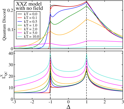
Figure 3: (color online) Quantum discord, Eq. (2), and the logarithm of the spectrum, Eq. (11), as a function of $\Delta$ for several values of temperature. For the upper panel, the temperature increases from top to bottom between the QCPs, while for the lower panel, it increases from bottom to top. Here and in all other graphs all quantities are dimensionless.

Note also that the QD is able to pinpoint the correct location of the QCPs up to $kT=10.0$. This is clearly seen by looking at Fig. 4, where we can better appreciate the cusps of $\mathcal{QD}$ at the two QCPs. And, as expected for a reasonable QCP detector, as we increase $T$ its efficacy decreases. This should be contrasted with the opposite behavior of $\mathcal{L}_{QC}^{x}$, being even “sharper” to detect a QCP for higher $T$. As it is clear now, this fact is due to its being ill-defined at the QCPs for this model.

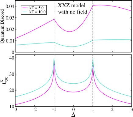
Figure 4: (color online) Same as Fig. 3, but now we focus on higher values of temperature.

In Fig. 5 we plot $\overline{\mathcal{F}}_{ext}$ and $\mathcal{S}_{QC}^{x}$. Both quantities now are bona fide QCP detectors.

Figure 5: (color online) Maximum mean fidelity, Eq. (51), and the coherence entropy, Eq. (10), as a function of $\Delta$ for several values of temperature. In both panels the temperature increases from top to bottom.

For $T=0$ they are both discontinuous at $\Delta=-1$, while at finite $T$ it is only $\overline{\mathcal{F}}_{ext}$ that has a discontinuous first order derivative at this QCP. This feature is also present for $\overline{\mathcal{F}}_{ext}$ at the second QCP, either at $T=0$ or when $T>0$. On the other hand, $\mathcal{S}_{QC}^{x}$ is less sharp to pinpoint the second QCP when compared with its ability to detect the first one. Also, when we increase $T$, $\mathcal{S}_{QC}^{x}$ loses its ability to detect both QCPs before this happens with $\overline{\mathcal{F}}_{ext}$. This is clearly depicted in Fig. 6.

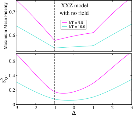
Figure 6: (color online) Same as Fig. 5, but now we focus on higher values of temperature. Note that the first order derivatives of $\overline{\mathcal{F}}_{ext}$ are still discontinuous at both QCPs while for $\mathcal{S}_{QC}^{x}$ no clear indication for the QCPs can be seen.

The results presented for this model are very illustrative of a general trend that will show up in the following ones. The most important message so far is that $\mathcal{L}_{QC}^{K}$, the logarithm of the spectrum, should not be considered a reliable QCP detector. It is unbounded and ill-defined when at least one of the eigenvalues of the operator $[\rho_{23},K]^{2}$ is zero. This happens for this model exactly in the QCPs and it is a consequence of the symmetry of the Hamiltonian and not a particular ability of $\mathcal{L}_{QC}^{K}$ to detect QCPs. Indeed, we showed that this feature, the existence of null eigenvalues, will persist even when $T\rightarrow\infty$. This means that $\mathcal{L}_{QC}^{K}$ diverges at the two QCPs for this model no matter how high the temperature is, a clear indication that $\mathcal{L}_{QC}^{K}$ cannot be considered a useful or well-defined QCP detector.

Second, the other quantities studied here are all bona fide QCP detectors. They share key characteristics of all known QCP detectors, namely, they are bounded and their efficacy to pinpoint a QCP diminishes as we increase the temperature. Two of these quantifies, the teleportation based QCP detector and the quantum discord, are more robust to temperature increases than the other one, the coherence entropy $\mathcal{S}_{QC}^{K}$. However, disregarding the issue of scalability for high spin systems and their operational meaning, from a strictly theoretical point of view they tend to complement each other in the investigation of QCPs as we will show next for the other models.

III.2 The XXZ model in an external field

Using the same notation and conventions given in Sec. III.1, the Hamiltonian for the XXZ model in the presence of an external longitudinal magnetic field is yan66 ; clo66 ; klu92 ; bor05 ; boo08 ; tri10 ; tak99

$$H=\sum_{j=1}^{L}\left(\sigma^{x}_{j}\sigma^{x}_{j+1}+\sigma^{y}_{j}\sigma^{y}_{j+1}+\Delta\sigma^{z}_{j}\sigma^{z}_{j+1}-\frac{h}{2}\sigma^{z}_{j}\right),$$ (56)

with $h$ denoting the external magnetic field.

For a finite magnetic field $h$, the ground state of this model has two QCPs yan66 ; clo66 ; klu92 ; bor05 ; boo08 ; tri10 ; tak99 . At the first one, $\Delta_{1}$, the ground state changes from a ferromagnetic ($\Delta<\Delta_{1}$) to a critical antiferromagnetic phase ($\Delta_{1}<\Delta<\Delta_{2}$). At the second one, $\Delta_{2}$, it becomes an Ising-like antiferromagnet for $\Delta>\Delta_{2}$.

The value of $\Delta_{1}$ is related to the external field by the following expression,

$$h=4J(1+\Delta_{1}),$$ (57)

while $\Delta_{2}$ is computed once we know $h$ by solving the following equation,

$$h=4\sinh(\eta)\sum_{j=-\infty}^{\infty}\frac{(-1)^{j}}{\cosh(j\eta)},$$ (58)

where $\eta=\cosh^{-1}(\Delta_{2})$.

In Table 1 we give the solutions to Eqs. (57) and (58) for $h=12.0$, the external field we will be using in this work. We should note, nevertheless, that the results here reported are quite general, being valid for other fields too pav23 ; pav24 . For comparison, we also provide in Table 1 the two QCPs when we have no field (the model we studied in the previous section).

Table 1: Quantum critical points $\Delta_{1}$ and $\Delta_{2}$ for the case of no field and when the external field is $h=12.0$. When $h=12.0$, $\Delta_{2}$ listed below is accurate within a numerical error of $\pm 0.001$.

	$h=0$	$h=12$
$\Delta_{1}$	-1.00	2.00
$\Delta_{2}$	1.00	4.875

When we turn on the longitudinal field, the magnetization $z$ is no longer null but we still have $xx=yy$. In this case, the four eigenvalues used to compute $\mathcal{S}_{QC}^{x}$ and $\mathcal{L}_{QC}^{x}$ are

$$\alpha_{1,2}^{x} = -\frac{1}{4}\left(zz+\sqrt{xx^{2}+z^{2}}\right)^{2},$$ (59)

$$\alpha_{3,4}^{x} = -\frac{1}{4}\left(zz-\sqrt{xx^{2}+z^{2}}\right)^{2}.$$ (60)

Similar to the case with no field, we still have that $\mathcal{S}_{QC}^{x}=\mathcal{S}_{QC}^{y}$ and $\mathcal{L}_{QC}^{x}=\mathcal{L}_{QC}^{y}$. This happens because the eigenvalues defining those quantities are all equal. We also have that the eigenvalues, Eqs. (59) and (60), are all negative.

In Fig. 7 we show $\mathcal{QD}$ and $\mathcal{L}_{QC}^{x}$ assuming a field of $h=12.0$.

Figure 7: (color online) Quantum discord, Eq. (2), and the logarithm of the spectrum, Eq. (11), as a function of $\Delta$ for several values of temperature when $h=12.0$. For the upper panel, the temperature increases from top to bottom between the QCPs, and for the lower panel, it increases from top to bottom when $\Delta<\Delta_{1}$.

The problematic definition of $\mathcal{L}_{QC}^{x}$ now manifests itself in two different places. First, for $\Delta<\Delta_{1}$, numerical analysis shows that $\alpha_{3,4}^{x}$ tends monotonically to zero as $\Delta\rightarrow-\infty$. Moreover, the lower $T$ the faster $\alpha_{3,4}^{x}$ approaches zero. This is why we see those extremely high values for $\mathcal{L}_{QC}^{x}$ when $\Delta<\Delta_{1}$. Second, between the two QCPs there is a value of $\Delta$ such that $\alpha_{1,2}^{x}\rightarrow 0$ and thus $\mathcal{L}_{QC}^{x}$ becomes undefined at this point. This is the reason for the cusps between the two QCPs that is not associated to any QPT seen in all curves for $\mathcal{L}_{QC}^{x}$.

The curves for QD also has a cusp between the two QCPs that are not related to a QPT. This is related to the minimization procedure of the quantum conditional entropy appearing in its definition wer10 ; wer10b . In the present notation, it is related to a discontinuous change in the optimal value of $\theta$ that minimizes Eq. (2). However, as we increase $T$ this cusp smooths out and disappear while for $\mathcal{L}_{QC}^{x}$ the cusp is always there.

At $T=0$, the curve for the QD as a function of $\Delta$ has discontinuous derivatives exactly at the two QCPs. These cusps are smoothed out and displaced away from the correct location of the QCPs as we increase $T$. The curves for $\mathcal{L}_{QC}^{x}$ behave similarly in the vicinity of the QCPs.

In Fig. 8 we show $\overline{\mathcal{F}}_{ext}$ and $\mathcal{S}_{QC}^{x}$ when $h=12.0$ for several values of $T$.

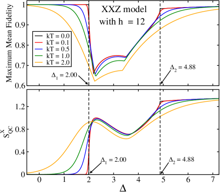
Figure 8: (color online) Maximum mean fidelity, Eq. (51), and the coherence entropy, Eq. (10), as a function of $\Delta$ for several values of temperature when $h=12.0$. For the upper panel, the temperature increases from top to bottom when $\Delta<\Delta_{1}$. For the lower panel, it increases from bottom to top when $\Delta<\Delta_{1}$.

Looking at the curves of $\overline{\mathcal{F}}_{ext}$ and $\mathcal{S}_{QC}^{x}$ when $T=0$, we note that the QCPs are all detected by discontinuities in the derivatives of those quantities as a function of $\Delta$. As we increase $T$, those discontinuous derivatives (cusps) are smoothed out and displaced from the correct spot of the QCPs. We should also note that $\overline{\mathcal{F}}_{ext}$ has two extra cusps between the two QCPs that are related to the maximization over the sets $S_{k}$ of unitary operations available to Bob pav23 ; pav24 . These extras cusps are not related to QPTs and they are located around the local maxima and minima seen in the curves for $\mathcal{S}_{QC}^{x}$ between the two QCPs.

In Fig. 9 we show $\overline{\mathcal{D}}_{int}$, the minimum mean trace distance for the internal teleportation protocol, as a function of $\Delta$. We have fixed the field at $h=12.0$ and plotted $\overline{\mathcal{D}}_{int}$ for several values of $T$.

Figure 9: (color online) Minimum mean trace distance, Eq. (52), as a function of $\Delta$ for several values of temperature when $h=12.0$. The temperature increases from bottom to top when $\Delta<\Delta_{1}$.

In Fig. 9 we see that for $T=0$ the QCPs are detected by discontinuities in the derivatives of $\overline{\mathcal{D}}_{int}$ with respect to $\Delta$ (see the kinks at $\Delta_{1}$ and $\Delta_{2}$). Contrary to $\overline{\mathcal{F}}_{ext}$, we now have only one tiny kink between the two QCPs that is not associated with a QPT. Similarly to the origin of the two extra kinks of $\overline{\mathcal{F}}_{ext}$, the single extra kink of $\overline{\mathcal{D}}_{int}$ can be traced back to the minimization over the sets $S_{k}$ of unitary operations pav24 . When $T>0$, the kinks related to the two QCPs are smoothed out and displaced from the exact locations of the QCPs. The extra kink between the two QCPs is also displaced from its $T=0$ spot but not appreciably smoothed out in the ranges of temperatures shown in Fig. 9.

In order to be more quantitative, we now compare the efficacy of the above quantities in estimating the correct values for the QCPs with finite $T$ data alone. We adopt the same techniques fully described in Refs. wer10b ; pav23 ; pav24 in the following analysis.

Although for finite $T$ the kinks are smoothed out, we still have an abrupt change in the value of those quantities about the QCPs. As such, for a fixed $T$, we compute the derivatives of those curves with respect to $\Delta$ about the QCPs. Then we pick the value of $\Delta$ giving the greatest magnitude for the derivatives. This $\Delta$ is considered the best approximation to the value of the QCP at that fixed $T$. Repeating this procedure for several temperatures, we can extrapolate to $T=0$ and correctly arrive at the exact values for the QCPs.

We work with six different temperatures, i.e., $kT=0,0.1,0.2,0.3,0.4,0.5$. For each one of these temperatures, we compute as a function of $\Delta$ and in increments of $0.01$ the several quantities shown in Fig. 10. Then, about $\Delta_{1}$, we numerically evaluate the first order derivatives of those quantities, picking the value of $\Delta$ that gives the greatest magnitude for the derivatives. About $\Delta_{2}$, we numerically compute the second order derivatives of those quantities, picking again the value of $\Delta$ giving the greatest magnitude for the second order derivatives. The values of those $\Delta$’s are plotted in Fig. 10.

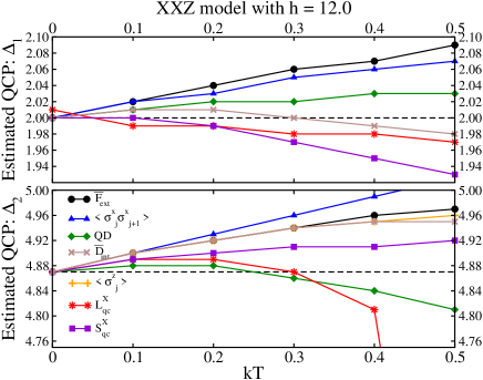
Figure 10: (color online) Estimated QCPs using finite $T$ data according to the procedure explained in the main text. For each value of $kT$, and for $f=\mathcal{QD},\mathcal{S}_{QC}^{x},\mathcal{L}_{QC}^{x},\overline{\mathcal{F}}_{ext},\overline{\mathcal{D}}_{int},$ $\langle\sigma^{x}_{j}\sigma^{x}_{j+1}\rangle,\langle\sigma^{z}_{j}\rangle$ (see legend), the upper panel gives the values of $\Delta$ related to the extrema of $df/d\Delta$ and the lower panel the values of $\Delta$ associated with the extrema of $d^{2}f/d\Delta^{2}$. The dashed lines mark the exact values of the QCPs. See text for details.

In numerically computing those derivatives, we used the forward difference method, namely, $df(x)/dx\approx[f(x+\eta)-f(x)]/\eta$, where $\eta=0.01$. Also, since $\Delta$ was changed in steps of $0.01$, the spot of the maxima of the absolute value of the first order derivatives have a numerical error of $\pm 0.01$. For the second order derivatives, which are computed from the first order ones, we have that the errors related to the location of their extrema are at least $\pm 0.02$ pav23 ; pav24 .

Looking at the upper panel of Fig. 10, we realize that the internal teleportation based QCP detector ($\overline{\mathcal{D}}_{in}$) outperforms all quantities in estimating the QCP $\Delta_{1}$ when $kT\geq 0.2$. For $kT\leq 0.2$, and taking into account the numerical error ($\pm 0.01$) for the values of the estimated QCP, we have that the QD, $\overline{\mathcal{D}}_{in}$, $\mathcal{S}_{QC}^{x}$, and $\mathcal{L}_{QC}^{x}$ are all equivalent in estimating the correct value of $\Delta_{1}$. Moreover, all quantities tend to the correct value of the QCP more or less linearly below a certain value of $kT$.

Moving our attention to the lower panel of Fig. 10, we note that the quantum discord ($\mathcal{QD}$) stands out as the optimal choice to estimate the correct value of $\Delta_{2}$, the second QCP. This is true for all the temperature range shown in Fig. 10. Taking into account that now the numerical error is at least $\pm 0.02$ for the estimated value of $\Delta_{2}$, below $kT\approx 0.1$ we have that the QD is equivalent to $\mathcal{S}_{QC}^{x}$ and $\mathcal{L}_{QC}^{x}$ in estimating the second QCP. We should also note that $\mathcal{L}_{QC}^{x}$ is almost useless to estimate the second QCP for $kT\geq 0.4$, providing very poor estimates.

Before we move on, we should note that this case, which was not studied in Ref. li20 , clearly illustrates that $\mathcal{L}_{QC}^{x}$ is not the optimal QCP detector. For this model, the internal teleportation based QCP detector is the best choice to estimate $\Delta_{1}$ while the QD is the best choice for estimating $\Delta_{2}$ when only finite $T$ data are available.

III.3 The XY model

Following the notation and boundary conditions already explained for the previous models, the Hamiltonian for the one-dimensional XY model subjected to a transverse magnetic field is lie61 ; bar70 ; bar71 ,

$$H\!=\!-\frac{\lambda}{4}\!\sum_{j=1}^{L}\!\left[(1+\gamma)\sigma^{x}_{j}\sigma^{x}_{j+1}+(1-\gamma)\sigma^{y}_{j}\sigma^{y}_{j+1}\right]\!-\frac{1}{2}\!\sum_{j=1}^{L}\!\sigma^{z}_{j}.$$ (61)

Here $\lambda$ is related to the inverse of the external magnetic field strength and $\gamma$ is the anisotropy parameter. When $\gamma=\pm 1$ we obtain the transverse Ising model and when $\gamma=0$ we get the isotropic XX model in a transverse field.

If we fix $\gamma$ and change $\lambda$, i.e., if we change the external field, we have a QCP at $\lambda_{c}=1.0$. This is the Ising transition. For $\lambda<1$ the ground state is an ordered ferromagnet while for $\lambda>1$ it becomes a quantum paramagnet pfe70 . If we now fix $\lambda$ such that $\lambda>1$, we also have another QPT if we change $\gamma$. It is the anisotropy transition, whose QCP is located at $\gamma_{c}=0$ lie61 ; bar70 ; bar71 ; zho10 . In this case, one of the phases is an ordered ferromagnet in the x-direction while the other phase is an ordered ferromagnet in the y-direction. These two QPTs belong to different universality classes lie61 ; bar70 ; bar71 ; zho10 .

For arbitrary values of $\lambda$ and $\gamma$, the density matrix describing a pair of spins for this model is given by Eqs. (1) and (44)-(48). In general we have all two-point correlation functions different ($xx\neq yy\neq zz$) and a non-null magnetization ($z\neq 0$). Therefore, using Eqs. (44)-(48), we can write Eqs. (17) and (18), the eigenvalues defining $\mathcal{S}_{QC}^{z}$ and $\mathcal{L}_{QC}^{z}$, as follows,

$$\alpha_{1,2}^{z} = -(xx+yy)^{2}/4,$$ (62)

$$\alpha_{3,4}^{z} = -(xx-yy)^{2}/4.$$ (63)

Note that the authors of Ref. li20 did not work with $\mathcal{S}_{QC}^{x,y}$ and $\mathcal{L}_{QC}^{x,y}$ for this model.

Again, all eigenvalues are negative and for non zero two-point correlation functions, two of them become zero if $|xx|=|yy|$. If we look at Eqs. (54) and (55), we realize that $\alpha_{1,2}^{z}$ and $\alpha_{3,4}^{z}$ have the same functional form of $\alpha_{1,2}^{x}$ and $\alpha_{3,4}^{x}$, the eigenvalues related to the XXZ model with no field. Indeed, changing $yy$ by $zz$ in the above expressions for the eigenvalues leads to the ones given by Eqs. (54) and (55). Therefore, the analysis we have made in Sec. III.1 about certain symmetries of the Hamiltonian and the equality of a pair of two-point correlation functions for any temperature applies here. As we show next, the alleged “robustness” of $\mathcal{L}_{QC}^{z}$ in detecting the $\gamma$-transition is associated with a particular symmetry of the Hamiltonian and to the ill-defined character of $\mathcal{L}_{QC}^{z}$. In other words, once more this example will illustrate that there is nothing outstanding in $\mathcal{L}_{QC}^{z}$ that sets it apart from other QCP detectors.

III.4 The $\gamma$ transition

The anisotropy transition occurs at $\gamma_{c}=0$. At this QCP, the Hamiltonian (61) becomes

$$H=-\frac{\lambda}{4}\!\sum_{j=1}^{L}\!\left[\sigma^{x}_{j}\sigma^{x}_{j+1}+\sigma^{y}_{j}\sigma^{y}_{j+1}\right]\!-\frac{1}{2}\!\sum_{j=1}^{L}\!\sigma^{z}_{j}.$$ (64)

Looking at Eq. (64), it is obvious that the two-point correlation functions $xx$ and $yy$ are equal. This happens because of the invariance of the Hamiltonian for rotations around the $z$-axis when $\gamma=0$.

Since $xx=yy$ for any $T$, we immediately see from Eq. (63) that $\alpha_{3,4}^{z}=0$ for any value of temperature. In other words, $\mathcal{L}_{QC}^{z}$ will diverge at $\gamma=0$ no matter how high the temperature is. This is the reason for the “robustness” of $\mathcal{L}_{QC}^{z}$ to temperature increases reported in Ref. li20 . As we understand now, this robustness is misleading. It is simply a consequence of the ill-defined character of $\mathcal{L}_{QC}^{K}$ when any one of the eigenvalues appearing in its definition becomes zero.

In Fig. 11 we show for several values of temperature $\mathcal{L}_{QC}^{z}$ and the other relevant QCP detectors, namely, $\mathcal{S}_{QC}^{z},\mathcal{QD},$ and $\overline{\mathcal{F}}_{ext}$, as functions of $\gamma$. We fix $\lambda=1.5$ in all those curves.

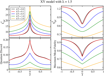
Figure 11: (color online) The several QCP detectors investigated in this work as a function of $\gamma$. We fixed $\lambda=1.5$ in Hamiltonian (61). In the top-left panel, temperature increases from bottom to top. In the remaining panels, temperature increases from top to bottom. See text for details.

Looking at Fig. 11, we realize that all quantities are useful in spotlighting the QCP up to $kT=2.0$. The QD and the external teleportation QCP detector (lower panels) spotlight the QCP by discontinuities in their first order derivatives with respect to $\gamma$ at the exact location of the QCP (see the kinks at $\gamma_{c}=0$). Those kinks are not displaced as we increase $T$ but become smoother. On the other hand, $\mathcal{S}_{QC}^{z}$ does not have those kinks. The QCP in this case is detected by noting that the global minimum of $\mathcal{S}_{QC}^{z}$ occurs at $\gamma_{c}=0$. Finally, $\mathcal{L}_{QC}^{z}$ diverges at the location of the QCP for any $T$ due to the reasons given above.

III.5 The $\lambda$ transition

The only case studied in Ref. li20 related to the $\lambda$ transition was the Ising transverse model ($\gamma=\pm 1.0$). For definiteness, here we fix $\gamma=1.0$ in the following analysis.

In Figs. 12 and 13 we plot the QD, $\mathcal{L}_{QC}^{z}$, $\overline{\mathcal{F}}_{ext}$ and $\mathcal{S}_{QC}^{z}$ as functions of $\lambda$ for several values of $T$. At $T=0$, the QCP is given by inflection points of these quantities at $\lambda_{c}=1.0$. As we increase $T$, the inflection points move away from the QCP and become less prominent as we increase $T$.

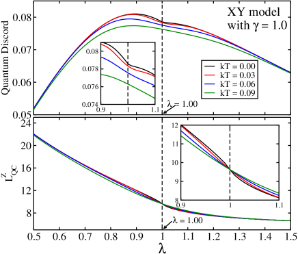
Figure 12: (color online) Quantum discord, Eq. (2), and the logarithm of the spectrum, Eq. (11), as a function of $\lambda$ for several values of temperature. Here we fix $\gamma=1.0$ (Ising transverse model). In all panels, the temperature increases from top to bottom when $\lambda<1.0$. The insets zoom in at the QCP, where in the $x$-axis we have $0.9\leq\lambda\leq 1.1$.

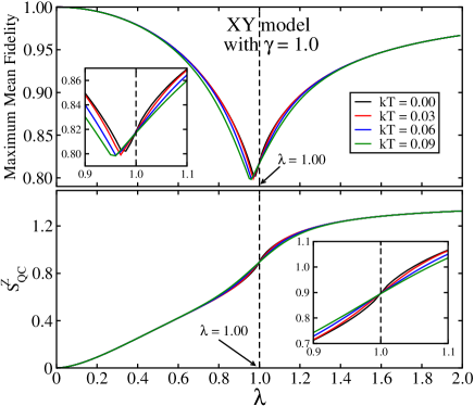
Figure 13: (color online) Maximum mean fidelity, Eq. (51), and the coherence entropy, Eq. (10), as a function of $\lambda$ for several values of temperature. Here we fix $\gamma=1.0$. In both panels the temperature increases from top to bottom after $\lambda>1.0$.

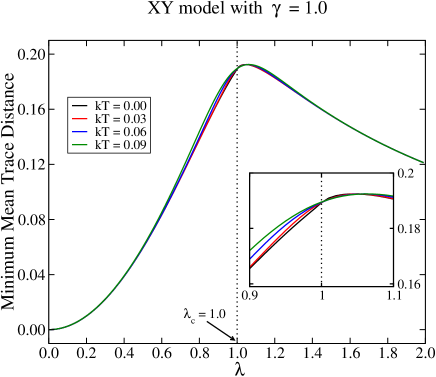
Figure 14: (color online) Minimum mean trace distance, Eq. (52), as a function of $\lambda$ for several values of temperature when $\gamma=1.0$. The temperature increases from bottom to top when $\lambda<1.0$. The inset zooms in at the QCP, where in the $x$-axis we have $0.9\leq\lambda\leq 1.1$.

Figure 14 illustrates the behavior of $\overline{\mathcal{D}}_{int}$ as a function of $\lambda$ for several values of $T$ and with $\gamma=1.0$. At $T=0$, it is now $d\overline{\mathcal{D}}_{int}/d\lambda$ that has an inflection point at the QCP pav24 . Similarly to the above cases, the higher $T$ the more distant from the QCP the inflection point is and it also becomes less prominent as we increase $T$.

To quantitatively compare the performance of these QCP detectors when only finite $T$ data are available, we repeat here the same analysis carried out for the XXZ model in an external field (see Sec. III.2). We now work with eleven different temperatures. We start at $kT=$ $0$ and go up to $kT=0.1$ in increments of $0.01$. For each value of $kT$, we compute the first and second order derivatives with respect to $\lambda$ for all the five QCP detectors shown in Figs. 12-14. In Fig. 15 we only show the corresponding estimate for the QCP extracted from the derivative (first or second order) leading to the best performance for each one of those quantities. As in Sec. III.2, the critical point is estimated by picking the value of $\lambda$ giving the greatest magnitude of the respective derivative around the exact $T=0$ location of the QCP.

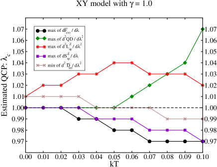
Figure 15: (color online) Estimated QCPs using finite $T$ data according to the procedure given in the main text. For each value of $kT$, we plot the values of $\lambda$ yielding the maximum of $df/d\lambda$, where $f=\overline{\mathcal{F}}_{ext},\mathcal{S}_{QC}^{z}$, and the values of $\lambda$ giving the maximum of $d^{2}f/d\lambda^{2}$, where $f=\mathcal{QD},\overline{\mathcal{D}}_{int},\mathcal{L}_{QC}^{z}$. The dashed line marks the exact location of the QCP. See text for details.

Contrary to what we did in Sec. III.2, we numerically computed those derivatives using the central difference method, namely, $df(x)/dx\approx[f(x+\eta)-f(x-\eta)]/(2\eta)$, where $\eta=0.01$. Both methods are equally valid but we opted now to work with the central difference method to contrast it with the curve of Ref. pav24 , where the forward difference method was used to compute $\overline{\mathcal{D}}_{int}$. Since $\lambda$ was changed in steps of $0.01$, both methods will differ by at least $0.01$ in giving the maximum for the magnitude of the derivatives. This is an illustrative example showing that the results reported here and in Ref. pav23 ; pav24 are accurate by at most the step $\eta=0.01$ used to generate the curves (see Appendix for more details). Furthermore, the same numerical errors related to the first and second order derivatives reported in Sec. III.2 apply here. The spot of the maxima of the absolute value of the first and second order derivatives have a numerical error of $\pm 0.01$ and $\pm 0.02$, respectively pav23 ; pav24 .

Looking at Fig. 15, we note that within the numerical errors (up to $\pm 0.02$ for the second derivatives), all quantities but $\mathcal{L}_{QC}^{z}$ give the correct location of the QCP for $kT\leq 0.4$. Moreover, within an error of $\pm 0.01$, the internal teleportation based QCP detector ($\overline{\mathcal{D}}_{int}$) gives the correct value of the QCP for all temperatures shown in Fig. 15. Again, the bottom line is that neither $\mathcal{S}_{QC}^{z}$ nor $\mathcal{L}_{QC}^{z}$ stands out as the most efficient QCP detector when only finite $T$ data are at stake.

IV Conclusion

We analyzed qualitatively and quantitatively the efficacy of different tools to detect quantum critical points (QCPs) for several classes of quantum phase transitions. In particular, we focused on the efficacy of those tools to properly identify a QCP when we only have access to finite temperature data. We worked with the following quantities, namely, the quantum discord oll01 ; hen01 ; wer10 ; wer10b , the coherence entropy and the logarithm of the spectrum li20 , which are based on the the quantum coherence wig63 ; fan14 ; gir14 , and the external and internal teleportation based QCP detectors pav23 ; pav24 , built on top of the standard quantum teleportation protocol ben93 ; yeo02 ; rig17 .

We worked with several types of one dimensional spin-1/2 chains, whose ground states had at least two quantum phases. The spin chains were studied in the thermodynamic limit (infinite number of spins) and we assumed the spin chains to be in equilibrium with a heat bath at temperature $T$. The models we studied were the XXZ model with and without an external longitudinal magnetic field, the Ising transverse model, and the XY model in an external transverse magnetic field.

From the theoretical point of view, the most important ingredient needed to compute all the quantities above is the density matrix describing a pair of nearest neighbor spins from the chain. It can be completely determined once we know all the one- and two-point correlation functions for a given spin chain. After obtaining this density matrix as a function of the temperature and of the parameters of the system’s Hamiltonian, we were able to compute the above quantities in the vicinity of the QCPs for several different values of $T$. This allowed was to investigate quantitatively the accuracy of those QCP detectors in correctly spotlighting the location of a QCP using finite $T$ data.

The first major result we arrived at is related to the faulty definition of the logarithm of the spectrum $\mathcal{L}_{QC}^{K}$ li20 . We showed that it cannot be defined for several classes of two-qubit density matrices. Also, we showed that the alleged “robustness” of $\mathcal{L}_{QC}^{K}$ in spotlighting QCPs at finite $T$ is related to this ill-definedness and has nothing to do with an intrinsic robustness to detect QCPs. Indeed, we showed that for all the models investigated in Ref. li20 , with the exception of the Ising model, the locations of the QCPs are exactly where $\mathcal{L}_{QC}^{K}$ is ill-defined (it diverges). This is the underlying cause for its “robustness” in detecting a QCP. We also showed that $\mathcal{L}_{QC}^{K}$ may give us false alarms, being divergent (undefined) when no quantum phase transition is taking place.

The second major result is related to the fact that no single QCP detector outperforms all the others. The optimal QCP detector depends on the model, on the QCP, and on the temperature. However, almost always either the quantum discord or the teleportation based QCP detector is the optimal choice. For the Ising transverse model, though, when we have low temperatures the coherence entropy $\mathcal{S}_{QC}^{K}$ is as efficient as the quantum discord and the internal teleportation based QCP detector.

We end by noting that the comparative study among the QCP detectors here presented does not consider the computational complexity to calculate them, in particular for high spin systems, as well as their operational meaning and experimental feasibility. It is known that the quantum discord is not easily computed for high spin systems mal16 , being an NP-complete problem hua14 . This means that it becomes impracticable to compute the quantum discord as we increase the size of the system under investigation. Furthermore, the quantum discord does not have a direct operational meaning and no general procedure to its direct measurement is known. We also have that $\mathcal{L}_{QC}^{K}$ and $\mathcal{S}_{QC}^{K}$ li20 are not easily computed for high spins and that no direct way of measuring them is available pav23 . On the other hand, the teleportation based QCP detectors have a direct experimental meaning and are easily generalized to high spin systems pav23 ; pav24 . On top of that, the necessary experimental steps to the implementation of the teleportation based QCP detectors are already at hand ron15 ; bra19 ; xie19 ; noi22 ; xue22 ; mad22 ; xie22 ; gam17 ; ohn99 ; han03 ; zin10 ; pet22 .

*

Appendix A Forward and central difference methods

The forward difference method to numerically compute the derivative of a function at point $x$ is given by the following expression,

$$\frac{df(x)}{dx}\approx\frac{f(x+\eta)-f(x)}{\eta},$$ (65)

where $\eta$ is the numerical step used to generate point $x_{j+1}$ from point $x_{j}$. The central difference method, on the other hand, is given by

$$\frac{df(x)}{dx}\approx\frac{f(x+\eta)-f(x-\eta)}{2\eta}.$$ (66)

Applying twice either the forward method or the central method, we computed for each value of $kT$ in Fig. 16 the second derivative of $\overline{\mathcal{D}}_{int}$ with respect to $\lambda$, the driving term for the Ising transverse model of Sec. III.5. Then, we picked the value of $\lambda$ leading to the minimum of $d^{2}\overline{\mathcal{D}}_{int}/d\lambda^{2}$. The points in Fig. 16 are the $\lambda$’s giving the minima of $d^{2}\overline{\mathcal{D}}_{int}/d\lambda^{2}$ at each $kT$.

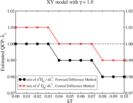
Figure 16: (color online) Estimated QCPs using finite $T$ data according to the procedure given in the main text. The two curves are obtained from two different finite difference methods to approximate the derivatives of $\overline{\mathcal{D}}_{int}$. The dashed line marks the exact value of the QCP ($\lambda_{c}=1.0$).

Looking at Fig. 16, we see that for every value of $kT$ the location of the minimum of $d^{2}\overline{\mathcal{D}}_{int}/d\lambda^{2}$, obtained by the central difference method, differs by $0.01$ from the location of the minimum determined via the other method. En passant, we should mention that if we had computed the derivatives using the backward difference method, where $df(x)/dx\approx[f(x)-f(x-\eta)]/\eta$, we would have obtained a curve that in Fig. 16 would appear displaced above the one for the central difference method by $\eta=0.01$. This will always happen because the derivative computed by the central difference method is the average of the values obtained by the forward and backward difference methods.

References

- (1) A. Osterloh, L. Amico, G. Falci, and R. Fazio, Nature (London) 416, 608 (2002).
- (2) T. J. Osborne and M. A. Nielsen, Phys. Rev. A 66, 032110 (2002).
- (3) L.-A. Wu, M. S. Sarandy, and D. A. Lidar, Phys. Rev. Lett. 93, 250404 (2004).
- (4) F. Verstraete, M. Popp, and J. I. Cirac, Phys. Rev. Lett. 92, 027901 (2004).
- (5) T. R. de Oliveira, G. Rigolin, M. C. de Oliveira, and E. Miranda, Phys. Rev. Lett. 97, 170401 (2006); T. R. de Oliveira, G. Rigolin, and M. C. de Oliveira, Phys. Rev. A 73, 010305 (2006); T. R. de Oliveira, G. Rigolin, M. C. de Oliveira, and E. Miranda, Phys. Rev. A 77, 032325(R) (2008).
- (6) R. Dillenschneider, Phys. Rev. B 78, 224413 (2008).
- (7) M. S. Sarandy, Phys. Rev. A 80, 022108 (2009).
- (8) G. Karpat, B. Çakmak, and F. F. Fanchini, Phys. Rev. B 90, 104431 (2014).
- (9) D. Girolami, Phys. Rev. Lett. 113, 170401 (2014).
- (10) M. Hotta, Phys. Lett. A 372, 5671 (2008).
- (11) M. Hotta, J. Phys. Soc. Jpn. 78, 034001 (2009).
- (12) K. Ikeda, Phys. Rev. D 107, L071502 (2023).
- (13) K. Ikeda, Phys. Rev. Appl. 20, 024051 (2023).
- (14) K. Ikeda, AVS Quantum Sci. 5, 035002 (2023).
- (15) K. Ikeda, R. Singh, and R.-J. Slager, e-print arXiv: 2310.15936 [quant-ph].
- (16) S. Sachdev, Quantum Phase Transitions (Cambridge University Press, Cambridge, 1999).
- (17) M. Greiner, O. Mandel, T. Esslinger, T. W. Hänsch, and I. Bloch, Nature (London) 415, 39 (2002).
- (18) V. F. Gantmakher and V. T. Dolgopolov, Phys. Usp. 53, 1 (2010).
- (19) S. Rowley, R. Smith, M. Dean, L. Spalek, M. Sutherland, M. Saxena, P. Alireza, C. Ko, C. Liu, E. Pugh et al., Phys. Status Solidi B 247, 469 (2010).
- (20) W. K. Wootters, Phys. Rev. Lett. 80, 2245 (1998).
- (21) T. Werlang and G. Rigolin, Phys. Rev. A 81, 044101 (2010).
- (22) T. Werlang, C. Trippe, G. A. P. Ribeiro, and G. Rigolin, Phys. Rev. Lett. 105, 095702 (2010); T. Werlang, G. A. P. Ribeiro, and G. Rigolin, Phys. Rev. A 83, 062334 (2011); T. Werlang, G. A. P. Ribeiro, and G. Rigolin, Int.J. Mod. Phys. B 27, 1345032 (2013).
- (23) Y. C. Li, J. Zhang, and H.-Q. Lin, Phys. Rev. B 101, 115142 (2020).
- (24) G. A. P. Ribeiro and G. Rigolin, Phys. Rev. A 107, 052420 (2023); G. A. P. Ribeiro and G. Rigolin, Phys. Rev. A 109, 012612 (2024).
- (25) G. A. P. Ribeiro and G. Rigolin, e-print arXiv:2403.10193 [quant-ph].
- (26) H. Ollivier and W. H. Zurek, Phys. Rev. Lett. 88, 017901 (2001).
- (27) L. Henderson and V. Vedral, J. Phys. A: Math. Gen. 34, 6899 (2001).
- (28) E. P. Wigner and M. M. Yanase, Proc. Natl. Acad. Sci. U.S.A. 49, 910 (1963).
- (29) C. H. Bennett, G. Brassard, C. Crepeau, R. Jozsa, A. Peres, and W. K. Wootters, Phys. Rev. Lett. 70, 1895 (1993).
- (30) Y. Yeo, Phys. Rev. A 66, 062312 (2002).
- (31) R. Fortes and G. Rigolin, Phys. Rev. A 96, 022315 (2017).
- (32) A. L. Malvezzi, G. Karpat, B. Çakmak, F. F. Fanchini, T. Debarba, and R. O. Vianna, Phys. Rev. B 93, 184428 (2016).
- (33) Y. Huang, New J. Phys. 16, 033027 (2014).
- (34) L. Ciliberti, R. Rossignoli, and N. Canosa, Phys. Rev. A 82, 042316 (2010).
- (35) Y. Huang, Phys. Rev. A 88, 014302 (2013).
- (36) M. A. Yurischev, Quantum Inf. Process. 14 3399 (2015).
- (37) S. Luo, Phys. Rev. A 72, 042110 (2005).
- (38) R. Fortes and G. Rigolin, Phys. Rev. A 92, 012338 (2015); 93, 062330 (2016).
- (39) A. Uhlmann, Rep. Math. Phys. 9, 273 (1976).
- (40) M. A. Nielsen and I. L. Chuang, Quantum Computation and Quantum Information (Cambridge University Press, Cambridge, 2000).
- (41) G. Gordon and G. Rigolin, Phys. Rev. A 73, 042309 (2006); 73, 062316 (2006); Eur. Phys. J. D 45, 347 (2007).
- (42) F. Toscano, D. G. Bussandri, G. M. Bosyk, A. P. Majtey, and M. Portesi, Phys. Rev. A 108, 042428 (2023).
- (43) D. G. Bussandri, G. M. Bosyk, and F. Toscano, Phys. Rev. A 109, 032618 (2024).
- (44) C. N. Yang and C. P. Yang, Phys. Rev. 147, 303 (1966).
- (45) J. Cloizeaux and M. Gaudin, J. Math. Phys. 7, 1384 (1966).
- (46) A. Klümper, Ann. Phys. 1, 540 (1992); Z. Phys. B 91, 507 (1993).
- (47) M. Bortz and F. Göhmann, Eur. Phys. J. B 46, 399 (2005).
- (48) H. E. Boos, J. Damerau, F. Göhmann, A. Klümper, J. Suzuki, and A. Weiße, J. Stat. Mech. (2008) P08010.
- (49) C. Trippe, F. Göhmann, and A. Klümper, Eur. Phys. J. B 73, 253 (2010).
- (50) M. Takahashi, Thermodynamics of one-dimensional solvable models (Cambridge University Press, Cambridge, 1999).
- (51) E. Lieb, T. Schultz, and D. Mattis, Ann. Phys. 16, 407 (1961).
- (52) E. Barouch, B. M. McCoy, and M. Dresden, Phys. Rev. A 2, 1075 (1970).
- (53) E. Barouch and B. M. McCoy, Phys. Rev. A 3, 786 (1971).
- (54) P. Pfeuty, Ann. Phys. (New York) 57, 79 (1970).
- (55) M. Zhong and P. Tong, J. Phys. A: Math. Theor. 43, 505302 (2010).
- (56) X. Rong, J. Geng, F. Shi, Y. Liu, K. Xu, W. Ma, F. Kong, Z. Jiang, Y. Wu, and J. Du, Nat. Commun. 6, 8748 (2015).
- (57) C. E. Bradley, J. Randall, M. H. Abobeih, R. C. Berrevoets, M. J. Degen, M. A. Bakker, M. Markham, D. J. Twitchen, and T. H. Taminiau, Phys. Rev. X 9, 031045 (2019).
- (58) T. Xie, Z. Zhao, X. Kong, W. Ma, M. Wang, X. Ye, P. Yu, Z. Yang, S. Xu, P. Wang et al., Sci. Adv. 7, eabg9204 (2021).
- (59) A. Noiri, K. Takeda, T. Nakajima, T. Kobayashi, A. Sammak, G. Scappucci, and S. Tarucha, Nature 601, 338 (2022).
- (60) X. Xue, M. Russ, N. Samkharadze, B. Undseth, A. Sammak, G. Scappucci, and L. M. Vandersypen, Nature 601, 343 (2022).
- (61) M. T. Mądzik, S. Asaad, A. Youssry, B. Joecker, K. M. Rudinger, E. Nielsen, K. C. Young, T. J. Proctor, A. D. Baczewski, A. Laucht et al., Nature 601, 348 (2022).
- (62) T. Xie, Z. Zhao, S. Xu, X. Kong, Z. Yang, M. Wang, Y. Wang, F. Shi, and J. Du, Phys. Rev. Lett. 130, 030601 (2023).
- (63) J. M. Gambetta, J. M. Chow, and M. Steffen, npj Quantum Inf. 3, 2 (2017).
- (64) Y. Ohno, R. Terauchi, T. Adachi, F. Matsukura, and H. Ohno, Phys. Rev. Lett. 83, 4196 (1999).
- (65) R. Hanson, B. Witkamp, L. M. K. Vandersypen, L. H. W. van Beveren, J. M. Elzerman, and L. P. Kouwenhoven, Phys. Rev. Lett. 91, 196802 (2003).
- (66) A. F. Zinovieva, A. V. Dvurechenskii, N. P. Stepina, A. I. Nikiforov, and A. S. Lyubin, Phys. Rev. B 81, 113303 (2010).
- (67) L. Petit, M. Russ, G. H. G. J. Eenink, W. I. L. Lawrie, J. S. Clarke, L. M. K. Vandersypen, and M. Veldhorst, Commun. Mater. 3, 82 (2022).