D-NPC: Dynamic Neural Point Clouds for
Non-Rigid View Synthesis from Monocular Video

Abstract

Dynamic reconstruction and spatiotemporal novel-view synthesis of non-rigidly deforming scenes recently gained increased attention. While existing work achieves impressive quality and performance on multi-view or teleporting camera setups, most methods fail to efficiently and faithfully recover motion and appearance from casual monocular captures. This paper contributes to the field by introducing a new method for dynamic novel view synthesis from monocular video, such as casual smartphone captures. Our approach represents the scene as a dynamic neural point cloud, an implicit time-conditioned point distribution that encodes local geometry and appearance in separate hash-encoded neural feature grids for static and dynamic regions. By sampling a discrete point cloud from our model, we can efficiently render high-quality novel views using a fast differentiable rasterizer and neural rendering network. Similar to recent work, we leverage advances in neural scene analysis by incorporating data-driven priors like monocular depth estimation and object segmentation to resolve motion and depth ambiguities originating from the monocular captures. In addition to guiding the optimization process, we show that these priors can be exploited to explicitly initialize our scene representation to drastically improve optimization speed and final image quality. As evidenced by our experimental evaluation, our dynamic point cloud model not only enables fast optimization and real-time frame rates for interactive applications, but also achieves competitive image quality on monocular benchmark sequences. Our project page is available at https://moritzkappel.github.io/projects/dnpc.

Figure 1: We introduce Dynamic Neural Point Clouds for dynamic view synthesis from monocular videos. Our method enables fast optimization, real-time frame rates, and competitive image quality.

1 Introduction

Synthesizing novel views from a sparse set of input images is a fundamental challenge in computer vision. Using recent advances in 3D neural scene reconstruction, it becomes possible to create photorealistic renderings from arbitrary viewpoints, effectively adding interactive six degrees-of-freedom camera support. In the context of general, non-rigidly deforming dynamic scenes, the capability of interactively rendering novel views for every point in time enables numerous applications, including video stabilization [28], immersive playback for social media [2], or virtual reality [57]. However, performing faithful reconstruction from just a single monocular video (e.g., a casual smartphone recording) remains a computationally expensive and challenging problem.

While the introduction of Neural Radiance Fields [31] and 3D Gaussian Splatting [19] brought about significant advances in static scene reconstruction, dynamic extensions still lag behind in terms of quality and robustness due to motion and depth ambiguities in the temporal domain. Those ambiguities are usually resolved using expensive large-scale multi view setups [24] or monocularized data (i.e., teleporting camera setups) [18], which maximize the ratio between camera and scene motion to improve temporal consistency. However, recent investigations [15] reveal that most sparsely regularized methods fail to faithfully recover consistent motion and geometry from casual smartphone captures due to the lack of effective multi-view signal. Multiple recent radiance field approaches address this problem by incorporating strong priors like monocular depth, optical flow, and semantic segmentation for the joint reconstruction of geometry, 4D scene flow fields [25, 26], and even camera parameters [27] from monocular video. While current monocular methods achieve high-quality spatiotemporally consistent view synthesis, they are often limited in the expressiveness of novel camera views, and by their high computational demand.

To address the above-mentioned challenges, this paper introduces Dynamic Neural Point Clouds (D-NPC), a new system for monocular dynamic view synthesis based on implicit point distributions and fast hash-encoded feature grids. Given a monocular input video and the corresponding structure-from-motion calibration, our method optimizes a 4D representation of the depicted scene, which enables spatio-temporal novel-view synthesis, e.g., the infamous bullet-time effect. Following the concept of implicit neural point clouds [17], we track expected scene density in a sparse voxel grid, which is used to extract explicit pose-dependent point clouds. Combined with a fast multi-resolution hash-encoded feature grid [33], this scene representation is able to efficiently render high-fidelity novel views using a differentiable rasterizer and image-to-image translation network. Based on the concepts of space-time hash encoding [51], we lift the representation to the temporal domain by replacing the single feature grid with a 3D and 4D hash encoding for the static background and dynamic foreground regions, respectively. We further extend the point distribution field to robustly track the per-voxel ratio of static and dynamic scene content, effectively enabling 3D dynamics segmentation to significantly reduce the required compute during optimization and inference.

To guide the severely under-constrained monocular reconstruction, we leverage per-frame data-driven priors, namely optical flow, monocular depth, and foreground segmentation masks, which we extract and preprocess with minimal overhead. We demonstrate that our temporal extension can take advantage of the rasterization-based forward rendering of implicit neural point clouds, which enables efficient foreground-background decomposition and image-space regularization. Furthermore, the scene-level sampling approach also provides a seamless way of integrating data-driven priors for model initialization, resulting in faster and better convergence during optimization. As shown in D-NPC: Dynamic Neural Point Clouds for Non-Rigid View Synthesis from Monocular Video, D-NPC achieves competitive image quality while significantly reducing optimization time, and allowing for interactive rendering in a graphical user interface.

Overall, we summarize our main technical contributions as follows:

• We propose a new, efficient dynamic scene representation for non-rigid scene reconstruction and novel-view synthesis from a single monocular input video. D-NPC is the first adaptation of implicit neural point clouds for dynamic view synthesis.

• We demonstrate that our model can elegantly leverage additional priors like monocular depth and object segmentation masks to explicitly initialize the sampling distribution field, which drastically improves optimization and inference speed.

Our method enables fast optimization in as few as 0.27 GPU hours and interactive frame rates above 60 FPS during inference, while achieving competitive image quality on common benchmark datasets.

2 Related Work

Rendering novel viewpoints of a recorded scene is a longstanding and well-studied problem. Early work on image-based rendering uses morphing to generate in-between views from image collections without explicit 3D reconstruction [9, 42]. Other approaches apply implicit or explicit 3D scene representations like light fields [16] or layered depth images [43] to generate high-quality novel views. Recently, Neural Radiance Fields (NeRFs) [31] and 3D Gaussian Splatting (3D-GS) [19] inspired a multitude of follow-up research, including extensions for dynamic scenes. We next briefly summarize neural representations for static scenes, followed by dynamic view synthesis.

2.1 Static View Synthesis

NeRFs [31] implicitly represent the scene geometry and appearance using a Multi-Layer Perceptron (MLP), yielding an unprecedented image quality for novel views at the cost of slow optimization and rendering due to the large number of network queries required. While some follow-ups propose qualitative improvements for, e.g., anti-aliasing and unbounded scenes [3, 4, 5], another branch of methods focuses on acceleration using explicit scene representations like sparse [13] or decomposed [8] voxel grids. Along the same lines, Müller et al. [33] propose an efficient grid-based scene representation implemented as a multi-resolution hash-grid, enabling high-quality reconstruction in only a few minutes. All the above volume rendering approaches apply backward rendering, where the scene is frequently sampled along the camera rays. In contrast, forward rendering approaches, explicitly model scene geometry using geometric primitives, allowing for fast rasterization-based rendering. The popular 3D-GS by Kerbl et al. [19] represents the scene as a set of 3D Gaussians for very fast rendering at a high image quality, inspiring many extensions [22, 60]. Analogously, point-based rendering approaches [1, 21, 39] use a fixed initial point cloud combined with a neural image translation network for hole filling. The recent INPC approach by Hahlbohm et al. [17] combines the benefits of forward and backward rendering, modelling the scene as a point probability and hash-encoded appearance field for high-quality rendering at interactive frame rates. Our D-NPC method leverages these benefits for fast dynamic view synthesis from monocular video. A more detailed discussion of neural rendering techniques can be found in the report by Tewari et al. [48].

2.2 Dynamic View Synthesis

Most NeRF-based extensions use a time-conditioned MLP [24, 25, 36] or additional deformation field [11, 34, 35, 37] to represent scene dynamics. Following acceleration models for static reconstruction, similar models based on factorized [2, 7, 12, 52] and hash-encoded [18, 45, 51] feature grids were introduced for dynamic view synthesis. D²NeRF [56] combined two models for foreground-background separation from a single video. Likewise, Wang et al. [51] decompose the scene in a fast 3D and 4D hash-grid representation. We adapt concepts from both approaches, integrating foreground/background handling in both our sampling and appearance modelling, enabling our method to individually render dynamic and static scene content while improving performance. Similar to radiance fields, recent approaches opt to extend 3D-GS for non-rigid scenes, tracking the 3D motion of Gaussians over time [29, 55] while retaining fast rendering. However, as recently revealed by Gao et al. [15], these methods require multi-view or monocularized [18] capturing setups to exploit observations from multiple views. On the other hand, multiple methods focus on dynamic view synthesis from a single monocular input video, integrating additional priors like dense scene flow estimation to resolve motion and depth ambiguities [25, 26, 27]. RoDynRF [27] further takes the challenging scenario to the extreme, additionally optimizing camera poses from the unposed input video. However, these MLP-based monocular approaches rely on backward rendering, thus being limited in optimization speed and final rendering frame rate. This paper presents a point-based forward rendering approach for monocular view synthesis, which leverages additional priors to initialize and guide the reconstruction, enabling high-quality rendering at real-time frame rates. More details on the state of the art in dynamic reconstruction can be found in the survey by Yunus et al. [61].

3 Method

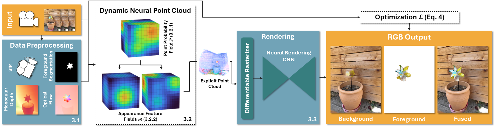
Figure 2: Method overview. Given a monocular RGB video and priors extracted from out-of-the-box estimators, we initialize and optimize a dynamic implicit neural point cloud, consisting of a spatiotemporal point position distribution and two feature grids for static and dynamic scene content. By sampling an explicit point cloud for a discrete timestamp, our model can synthesize novel views, including foreground/background separation, using a differentiable rasterizer and neural renderer.

We introduce Dynamic Neural Point Clouds (D-NPC), a method for dynamic novel-view synthesis from monocular video. Given a single monocular video consisting of $N$ images $I=(i_{1},...,i_{N})$ and their normalized timestamps $T=(t_{1},...,t_{N})\in[0,1]^{N}$, we reconstruct a dynamic implicit point cloud representation [17] of the depicted dynamic scene. Based on its static counterpart, the core of our D-NPC model consists of a spatiotemporal point probability ($\mathcal{P}$) and appearance feature descriptor ($\mathcal{A}$) field, which can efficiently be rendered using a differentiable rasterizer and neural rendering network. A full overview of our method is given in Fig. 2. In the following, we describe the individual components and optimization process in detail.

3.1 Data Preprocessing

The reconstruction of non-rigidly deforming scenes from a single moving camera is a highly ill-posed problem. To regularize the reconstruction from monocular video, previous approaches [15, 25, 27] apply estimates from several image processing applications, replacing the multi-view consistency signal with learned, data-driven scene analysis. Following this idea, our method starts with data preprocessing to extract high-quality priors, which we use to initialize and guide our model in the later stages. Despite the recent emergence of consistent yet expensive scene calibration [44], video depth estimation [30] and motion tracking [53] estimators, one of our method’s main objectives is speed and simplicity. Thus, we focus on real-time out-of-the-box solutions to maintain a fast total reconstruction time (including prior computation).

First, we start by applying sparse structure-from-motion (SfM) using COLMAP [40, 41] to estimate camera intrinsics and per-frame poses (extrinsics) $E=(e_{1},...,e_{N})$. As a side product, we extract the sparse, globally-aligned SfM point cloud. We further use RAFT [47] to estimate dense optical flow in the forward and backward directions, and estimate per frame (dis-)occlusion masks based on forward-backward consistency. To reduce the depth ambiguity of dynamic scene content, we employ the fast monocular depth estimator DepthAnything [58], which provides relative disparity maps for every video frame. Instead of using a relative depth loss [25], we align the predicted disparity with the global SfM point cloud by estimating a scale and shift via RANSAC-based least squares and temporal smoothing. This way, we obtain globally-aligned depth which can explicitly be integrated into our model. Lastly, we obtain binary segmentation masks $\omega$ of moving foreground object(s) to mask out dynamic scene content in our reconstruction and COLMAP SfM feature extraction. Similar to monocular depth, automatic motion segmentation is highly ill-posed, even in the presence of semantic segmentation masks. Thus, we use the semi-automatic video object segmentation system Cutie [10], which is guided by minimal user input in the form of manual keypoint selection. In line with our demands on simplicity, Cutie generates masks of sufficient quality in less than a minute, requiring as few as two mouse clicks, which in the future could be integrated into the data recording setup on mobile devices.

3.2 Dynamic Neural Point Cloud Representation

Our method represents the 4D scene as a Dynamic Neural Point Cloud, the first temporal extension of implicit neural point clouds [17]. The primary idea of implicit point clouds is to replace the persistent point cloud $(p,f)$, consisting of a set of 3D positions $p$ and corresponding color or feature descriptor vectors $f$, with a sampling distribution $\mathcal{P}$ and a neural feature grid $\mathcal{A}$. By repeatedly sampling and rendering an explicit point cloud $((p,\mathcal{A}(p)),p\sim\mathcal{P})$, it is possible to iteratively update and refine the spatial distribution, while maintaining all benefits of point-based rendering. However, applying this concept to dynamic scenes is not straightforward, as the direct integration of a fourth dimension is memory-intensive and does not naturally exploit any temporal coherency.

3.2.1 Temporal Point Probability Field

The probability field $\mathcal{P}$ models the likelihood for spatial point sampling by tracking the estimated local scene opacity $\sigma\in[0,1]$ over the course of optimization. To facilitate accurate and efficient sampling over a dynamic sequence, we divide our probability field $\mathcal{P}=(\mathcal{P}_{s},\mathcal{P}_{d})$ into two separate instances for static and dynamic regions, respectively. While the static 3D field $\mathcal{P}_{s}$ continues to track local opacity $\sigma_{s}$ assumed to be consistent over all points in time, the 4D dynamic field $\mathcal{P}_{d}$ stores additional values $\sigma_{d}(t)$ as a function of time. To enable a clean separation of foreground and background, $\mathcal{P}_{d}$ not only models the expected local opacity, but additionally keeps track of the estimated local proportion $\beta(t)$ between static and dynamic substance, as explained later on. In conjunction, our probability fields can sample explicit, time-aware point positions, while pre-marking individual points as either dynamic or static to reduce compute complexity. Given the natural imprecisions and relatively low resolution of monocular reconstruction, we find that the octree-based data structure suggested by Hahlbohm et al. [17] does not yield significant benefits due to the absence of fine geometric details. Instead, we use a fixed-resolution sparse voxel grid representation for the static and dynamic fields.

Voxel Grid Initialization.

Despite using a sparse data structure, starting from a fully occupied grid (i.e., all cells are sampled equally for all timestamps) is exceedingly inefficient regarding both memory consumption and model convergence. Thus, we make use of the data-driven priors described in Sec. 3.1 to find a sparse initial sampling distribution before optimization. First, we initialize the voxel grid bounds as the minimal cuboid enclosing all SfM points after performing outlier filtering based on the 95-percentile, containing a fixed total of $128^{3}$ and $N\cdot 128^{3}$ voxels for $\mathcal{P}_{s}$ and $\mathcal{P}_{d}$ respectively. Then, for every timestamp $t_{i}\in T$, we use the corresponding training camera matrix $e_{i}$ to project a set of random points in each voxel to the image plane, and gather the minimal relative distance to the estimated monocular depth $d_{i}$, and the maximum over the binary foreground segmentation mask $\omega_{i}$. We set the initial opacity-based sampling probability $\sigma_{d}(t_{i})$ of each cell to the relative deviation from the monocular depth, using the maximum over all timestamps for the static field ($\sigma_{s}=\max(\{\sigma_{d}(t)\>|\>t\in T\})$). Additionally, we carve the temporal slices of $\mathcal{P}_{d}$ using the dynamic segmentation. By thresholding the sampling probabilities, we eliminate up to 95% of voxels, resulting in an efficiently represented distribution constituting a proper local minimum for optimization.

Explicit Point Cloud Sampling.

For an arbitrary camera view $e$ and timestamp $t$, we sample a set $P\in\mathbb{R}^{k\times 3}$ of $k$ explicit point positions ($P\sim\mathcal{P}\>|\>(e,t)$) for rendering a novel view. To this end, we first take the union of all voxels in the static field and the dynamic field at time $t$, taking the maximum expected opacity of voxels existing in both models. Then, we eliminate voxels based on the camera frustum by projecting each voxel center to the image plane using $e$. To obtain the final point positions $p$, we interpret the per-voxel opacity as a discrete PDF, using discrete multinomial sampling (with replacement) to propose a list of voxels, in each of which we place a single uniformly sampled 3D position. This way, more points are sampled in areas with a high expected scene density, which can iteratively be refined during optimization. For the resulting set of point positions, we further trace a binary mask $m_{p}$ indicating if a point was sampled from static or dynamic scene regions, enabling efficient model evaluation by omitting excessive queries of the dynamic appearance model.

Voxel Grid Update.

We update the sampling distribution field by tracking the blending weights assigned to every sampled explicit point during rasterization. We first apply a constant decay factor to the values of every unique voxel proposed by the multinomial sampling, and then assign it the maximum over the current value and the blending weights of all points sampled from the specific cell. For samples from dynamic voxels of $\mathcal{P}_{d}$, we apply the same procedure to the tracked static-to-dynamic ratios $\delta$ using per-point densities described in Sec. 3.2.2. Afterwards, we prune voxels from the sampling distribution by threshold: For $\mathcal{P}_{d}$, we remove cells with a low $\delta$-value, as it either describes empty space or is well handled by the static model. We further remove voxels $\mathcal{P}_{s}$ from $\mathcal{P}_{d}$ whose expected opacity $\sigma$ is low in the static 3D field and for all remaining timestamps in the dynamic field. This way, we progressively reduce memory consumption and refine importance sampling.

3.2.2 Dynamic Appearance Field

In a conventional point cloud, every point is assigned a fixed feature vector describing its appearance. As implicit neural point clouds [17] repeatedly extract new sets of point positions, they use a fast multi-resolution hash-encoded feature grid [33] $\mathcal{A}$ to model the appearance over the entire spatial sampling distribution. To represent time-conditioned appearance for dynamic scenes, we again use a static 3D and dynamic 4D hash-encoded neural feature grid $\mathcal{A}=(\mathcal{A}_{s},\mathcal{A}_{d})$. As previously described by Wang et al. [51], using an ensemble of 3D and 4D hash-grids instead of a single 4D representation effectively improves the capabilities of the dynamic model by reducing hash collisions. To model the static and dynamic scene appearance at a spatial input position $p$ at time $t$, the appearance fields yield a density $\delta\in\mathbb{R}_{0}^{+}$ and an $n_{f}$-dimensional feature vector $f\in[0,1]^{n_{f}}$:

$$\delta_{s},f_{s}=\mathcal{A}_{s}(p),\quad\delta_{d},f_{d}=\mathcal{A}_{d}(p,t).$$ (1)

Note that we only have to query $\mathcal{A}_{d}$ for points indicated as dynamic by the binary segmentation mask $m$, which significantly reduces compute and memory. Following the formulation of D²NeRF [56], we then calculate the combined per-point density $\delta_{c}$ as the sum of static and dynamic densities, and obtain the final feature descriptor $f_{c}$ via density-weighted interpolation:

$$\delta_{c}=\begin{cases}\delta_{s}+\delta_{d}&\text{if}\quad m(p)\\ \delta_{s}&\text{else}\end{cases},\qquad f_{c}=\begin{cases}\frac{\delta_{s}f_{s}+\delta_{d}f_{d}}{\delta_{c}}&\text{if}\quad m(p)\\ f_{s}&\text{else}\end{cases}.$$ (2)

For rendering and probability field updates, we then transform density values $\delta$ into opacity $\sigma$, and calculate the dynamic ratio $\beta$ via:

$$\sigma_{(s/d/c)}=1-e^{-\delta_{(s/d/c)}},\quad\beta=\frac{\delta_{d}}{\delta_{c}}.$$ (3)

3.3 Neural Point Cloud Rendering

Given the time-dependent neural point cloud for an input view consisting of point positions $p$, point opacity $\sigma$, and appearance features $f$, we implement a fast differentiable point rasterizer to generate alpha ($\alpha$), depth ($d$), and 2D image feature maps $f_{\text{img}}$. Naturally, the rasterized images still contain holes, a common characteristic of classical point rendering approaches. Thus, we use a neural renderer, implemented as a light-weight convolutional neural network with a U-Net [38] architecture to fill the remaining holes, and convert the neural feature map $f_{\text{img}}$ to a human-interpretable RGB image $c$. In practice, we apply the rasterization and rendering components to the static, dynamic, and combined point cloud features separately, resulting in individual depth $d_{s,d,c}$ and color $c_{s,d,c}$ images that can be used for supervision and regularization. As the resolution of dynamic view synthesis benchmarks is usually low, we do not use any splatting or multi-resolution inputs in the rasterizer or neural renderer, which further increases performance.

3.4 Optimization

During training, we iteratively sample an explicit point cloud (Sec. 3.2.1) for a random training view and its associated timestamp, extract per-point appearance features (Sec. 3.2.2), render the resulting images (Sec. 3.3), update the sampling distribution (Sec. 3.2.1), and optimize model parameters using the following objective function:

$$\mathcal{L}=\lambda_{\text{photo}}\mathcal{L}_{\text{photo}}+\lambda_{\text{depth}}\mathcal{L}_{\text{depth}}+\lambda_{\text{seg}}\mathcal{L}_{\text{seg}}+\lambda_{\text{dist}}\mathcal{L}_{\text{dist}},$$ (4)

with hyperparameters $\lambda_{\text{photo}}$, $\lambda_{\text{depth}}$, $\lambda_{\text{seg}}$ and $\lambda_{\text{dist}}$. We use the same set of hyperparameters across all our experiments. The loss $\mathcal{L}_{\text{photo}}$ enforces photometric consistency between the rendered ($c$) and GT RGB image. Here, we use a weighted combination of pixel-level Cauchy loss [6], structural dissimilarity [54], and perceptual LPIPS [62] to maximize image quality. Our depth regularization loss $\mathcal{L}_{\text{depth}}$ penalizes the difference between the rasterized dynamic depth $d_{d}$ and the aligned monocular depth prior $d_{\text{gt}}$ in the binary foreground mask $\omega$:

$$\mathcal{L}_{\text{depth}}=\frac{1}{\lvert\omega\rvert}\sum_{i=0}^{\lvert\omega\rvert}\omega_{i}\lvert d_{d,i}-d_{\text{gt},i}\rvert.$$ (5)

The segmentation regularizer $\mathcal{L}_{seg}$ encourages a clean separation between the static and dynamic models via skewed binary entropy [56] on the dynamic ratios $\beta$:

$$\mathcal{L}_{\text{seg}}=-\beta^{k}\log_{2}(\beta^{k})-(1-\beta^{k})\log_{2}(1-\beta^{k}),$$ (6)

where $k$ is the skewing bias. As our last regularizer $\mathcal{L}_{dist}$, we adapt the distortion loss of Mip-NeRF360 [4, 46] to encourage thin surfaces, as it is not feasible to reliably reconstruct the time-dependent volume of a deforming object from a single monocular observation. For a detailed description of our training and loss schedule, please see our supplemental material (Sec. A.2).

4 Experimental Evaluation

We perform quantitative (Sec. 4.1) and qualitative (Sec. 4.2) evaluation and comparisons against state-of-the-art methods on two benchmark datasets: First, we evaluate our approach on the NVIDIA dynamic scenes dataset [59] (MIT license), featuring forward-facing scenes captured by a multi-view rig, monocularized by using a single frame per time to get a smooth camera trajectory. We extract training data using the procedure of RoDynRF [27], resulting in $12$ training and test views. For comparisons against DynIBaR [26] using their train/test split containing $\sim 150$ training views per scene, please see our supplemental material. Additionally, we evaluate our approach on the iPhone dataset [15] (Apache 2.0 license) which comprises challenging sequences with complex camera and scene motion trajectories, fine texture details, and (self-)occlusions. Furthermore, we provide an ablation study assessing the influence of individual pipeline components in Sec. 4.3.

4.1 Quantitative Results

Table 1: Timings on the NVIDIA dataset. We report training time and inference frame rates on the NVIDIA dataset with an image resolution of $480{\times}270$ pixels. Values for methods marked with $\dagger$ were gathered from the literature.

Method	GPU Hours [h] $\downarrow$	Frame Rate [FPS] $\uparrow$
RoDynRF [27]†	28	${<}1$
HyperNeRF [35]†	64	${<}1$
DynamicNeRF [14]†	74	${<}0.1$
NSFF [25]†	223	${<}1$
DynIBaR [26]†	320	${<}1$
4D-GS [55]	1.1	45
Ours	0.27	70

Table 2: Quantitative comparisons on the NVIDIA and iPhone datasets against recent dynamic view synthesis approaches. Our method achieves the best average scores in terms of perceptual image quality. The three best results are highlighted in green in descending order of saturation.

	NVIDIA Average
Method	PSNR $\uparrow$	SSIM $\uparrow$	LPIPS $\downarrow$
T-NeRF [37]	18.33	0.436	0.511
D-NeRF [37]	21.49	0.629	0.320
HyperNeRF [35]	17.60	0.377	0.502
NR-NeRF [49]	19.69	0.510	0.434
NSFF [25]	24.33	0.751	0.257
DynamicNeRF [14]	26.10	0.837	0.142
RoDynRF [27]	25.89	0.854	0.110
TiNeuVox [11]	19.74	0.501	0.412
4D-GS [55]	22.89	0.731	0.237
Ours	25.64	0.845	0.109

	iPhone Average
Method	mPSNR $\uparrow$	mSSIM $\uparrow$	mLPIPS $\downarrow$
HyperNeRF+B+D+S [35]	16.81	0.569	0.332
Nerfies+B+D+S [34]	16.45	0.570	0.339
T-NeRF [15]	15.70	0.538	0.458
T-NeRF+B+D [15]	17.06	0.573	0.390
T-NeRF+B+D+S [15]	16.96	0.577	0.379
RoDynRF [27]	17.00	0.535	0.517
4D-GS [55]	13.87	0.459	0.407
Ours	15.79	0.585	0.354
Ours${}_{\text{Lidar}}$	16.84	0.597	0.319

We compare the performance of several related methods in Tab. 1. For all NeRF-based approaches, we report values from the literature. To further compare against a fast forward rendering approach, we train the state-of-the-art Gaussian splatting-based 4D-GS [55] on both benchmark datasets. For both 4D-GS and our method, we measure performance on a single RTX 4090 GPU. As evident from the results, our method is significantly faster than backward rendering approaches, and even trains faster than 4D-GS while achieving similar frame rates during inference. A breakdown of timings for individual method components is provided in the supplemental material. We further compare image quality based on PSNR, SSIM [54] and LPIPS [62] quality metrics on the NVIDIA and iPhone datasets in Tab. 2. To avoid inconsistencies across the reported values, we use the official results and models kindly provided by Liu et al. [27], Li et al. [26], and Gao et al. [15] to consistently recalculate all metrics using the VGG backbone for LPIPS calculation. For the iPhone dataset, we use masked metric calculation (mPSNR, mSSIM, mLPIPS) as suggested and implemented by Gao et al. [15] to account for co-visibility. Overall, we find our method is not only the fastest in terms of reconstruction and rendering speed but also achieves competitive image quality, especially in terms of perceptual image quality metrics (LPIPS). While RoDynRF and T-NeRF achieve better per-pixel PSNR scores, we find that both methods fail to preserve high frequencies, resulting in an inferior perceived image quality, as shown in the next section. Detailed per-scene results can be found in our supplement.

4.2 Qualitative Results

TiNeuVox

RoDynRF

4D-GS

Ours

Ground Truth

Figure 3: Qualitative comparisons on the NVIDIA dataset. Our method preserves fine details and clean foreground-background transitions.

HyperNeRF$\dagger$

T-NeRF$\dagger$

RoDynRF

4D-GS

Ours

Ground Truth

Figure 4: Comparison on the iPhone dataset. We compare on two challenging scenes of the iPhone dataset. Our method better preserves the object shapes and fine details despite complex deformations. Methods indicated by $\dagger$ are the highest quality versions provided by Gao et al. [15]

We show qualitative results on the NVIDIA (Fig. 3) and iPhone (Fig. 4) datasets. For comparisons on the iPhone sequences, we show the best version of HyperNeRF [35] and T-NeRF [37] according to image quality metrics, using all additional regularizers (Lidar depth, random background, and distortion loss) proposed by Gao et al. [15]. For our method, we report values for two versions, trained with the provided Lidar or monocular depth data. Again, we find that our method achieves a competitive and oftentimes superior perceived image quality, preserving higher frequencies and clean edges. For dynamic view synthesis results, please see our supplemental video.

4.3 Ablation Study

Table 3: Comparison of ablated D-NPC versions in terms of image quality, model size and speed.

Method	Image Quality			Model Size	Frame Rate
	PSNR $\uparrow$	SSIM $\uparrow$	LPIPS $\downarrow$	[MB] $\downarrow$	[FPS] $\uparrow$
Oursfull	25.64	0.845	0.109	668	72
Oursw/o init	21.70	0.617	0.302	813	45
Oursw/o depth	24.40	0.835	0.135	671	72
Oursw/o U-Net	24.24	0.798	0.155	662	78

To assess the improvements enabled by our main pipeline components, we optimize three variations of our method on the NVIDIA dataset, and compare them to our full D-NPC model (full). First, we train our model from scratch without initializing the probability field from the monocular depth and foreground segmentation, just using camera frustum carving to reduce the amount of initial cells (w/o init). Additionally, we compare against a version without depth supervision during training (w/o depth), which is a crucial component in monocular dynamic view synthesis. Lastly, we evaluate the impact of our neural renderer by skipping the U-Net, directly interpreting the rasterized point cloud features as RGB outputs (w/o U-Net). As evident from Tab. 3, our initialization procedure effectively guides the model to a favorable representation, decreasing image quality and increasing memory when omitted. Likewise, skipping additional depth supervision from the globally aligned monocular depth maps significantly deteriorates reconstruction quality. The neural rendering network used for hole filling, while also contributing to improved final image quality, comes at the cost of a slightly decreased inference frame rate. We find that direct RGB rasterization without a rendering network can still produce visually appealing results, and improves the interactivity at higher resolutions when exploring scenes in a graphical user interface. Importantly, the U-Net weights do not have any significant impact on the final model size, which is dominated by the dynamic sampling and appearance parameters.

5 Discussion and Limitations

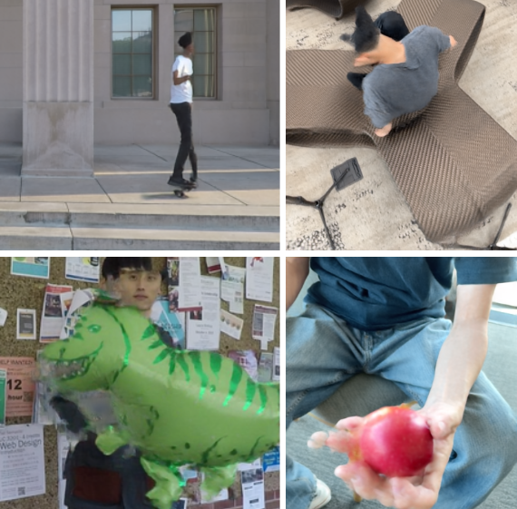
Figure 5: Failure Cases. Top: Cropped foreground not contained in the training camera frustum. Bottom: Object duplications due to depth misalignment.

In our experiments, our D-NPC yields the best trade-off between optimization time and image quality and is currently the only monocular method providing real-time frame rates for interactive applications. Especially in terms of perceptual LPIPS and high image frequencies, our method quantitatively and visually outperforms recent monocular view synthesis methods while only requiring a fraction of the optimization time. However, there is room for improvement: Our method relies on a decent quality of camera poses and monocular depth. Moreover, our initialization process assumes that the dynamic content is fully contained in the camera frustum, resulting in visible crops when synthesizing far-off novel views, as shown in Fig. 5.

6 Conclusion

We presented Dynamic Neural Point Clouds, an efficient implicit point cloud-driven [17] approach for non-rigid novel-view synthesis from monocular video inputs. In contrast to existing ray marching-based NeRF methods, our rasterization-based forward rendering approach enables a direct and elegant way to initialize and guide the reconstruction from data-driven priors, not only making it one of the fastest approaches in terms of optimization time, but also enabling rendering at real-time frame rates. While our experiments show our novel approach already yields competitive image quality according to several metrics on common benchmark datasets, we believe that our work constitutes a promising new direction for future research and extensions, like the integration of diffusion-based priors.

Appendix A Appendix – Supplemental Material

In this supplemental, we provide details on our model configuration (Sec. A.1) and optimization procedure (Sec. A.2), include additional results (Sec. A.3), and discuss concurrent work on arXiv (Sec. A.4) as well as the societal impact (Sec. A.5) of our work.

A.1 Model Details

Table 4: Appearance Field Hash Grid Configurations.

Parameter	3D Static Grid	4D Dynamic Grid
Base Resolution	16	16
Resolution Levels	10	8
Per Level Scale	2	2
Features Per Level	4	4
Logarithmic Size	21	22

In our model, the crucial neural components regarding the image quality are the appearance feature grids and the neural rendering network. To model our static and dynamic appearance fields, we use the fast multi-resolution hash encoding implementation by Müller et al. [33, 32] After initially carving our sampling distribution voxel grid using the monocular depth and dynamic segmentation priors, we set the spatial scale of our 3D and 4D feature grids to the minimum axis-aligned bounding box enclosing all remaining static and dynamic voxels, respectively. We parameterize the hash-grids according to the values in Tab. 4, giving more total capacity to the higher dimensional dynamic representation. Both hash encodings are followed by a shallow ReLU-activated MLP with one hidden $64$-neuron layer to resolve hash collisions.

For our neural rendering network used for hole-filling, we apply a simple image-to-image translation approach based on a U-Net architecture [38]. In contrast to Hahlbohm et al. [17], we do not use any multi-resolution inputs. Instead, we use two downsampling and consecutive upsampling blocks, each consisting of two ReLU-activated 2D convolutions with kernel size $3$, followed by average pooling / bilinear upsampling. During down- and upscaling, each convolution block doubles/halves the amount of feature channels while adjusting the spatial resolution, going from an initial $64$ channels at the finest to a maximum of $256$ channels at the coarsest spatial resolution.

A.2 Optimization Details

Table 5: Loss Hyperparameters.

Hyperparameter	Value
$\lambda_{\text{photo, Cauchy}}$	1.0
$\lambda_{\text{photo, D-SSIM}}$	0.9
$\lambda_{\text{photo, LPIPS}}$	0.05
$\lambda_{\text{depth}}$	20.0
$\lambda_{\text{seg}}$	$1\mathrm{e}{-3}$
$\lambda_{\text{dist}}$	1.0
$k$	0.5

We train our model for a total of 10K iterations on a consumer-grade RTX 4090 GPU. During each iteration, we sample an explicit point cloud consisting of $4$M points (i.e., a batch of spatial 3D locations). While the sampling distribution is manually updated based on statistics of the extracted explicit point clouds (see Sec. 3.2.1), the differentiable rasterizer and neural rendering network enable end-to-end optimization using gradient descent for the network and hash-grid parameters. We use the Adam [20] optimizer ($\beta_{1}=0.9$, $\beta_{2}=0.99$, $\epsilon=1\mathrm{e}{-15}$) with an initial learning rate of $1\mathrm{e}{-2}$ for the appearance hash-grids and $5\mathrm{e}{-4}$ for the rendering network, which are exponentially decayed to $\frac{1}{3}\mathrm{e}{-3}$ and $5\mathrm{e}{-5}$ during optimization. For our loss hyperparameters (Sec. 3.4), we use the values provided in Tab. 5. Note that, after initially training with a high value $\lambda_{depth}$ to guide the optimization in a reasonable direction, we turn off our depth loss after $500$ training iterations to allow the model to recover from errors in the monocular depth estimates. In contrast to D²NeRF, who use $k=2$ to bias the binary segmentation loss towards static background, which usually constitutes a majority of the scene, we use a value of $0.5$ to favor the dynamic model. This is due to the fact that our initialization procedure already discards large amounts of dynamic model evaluation in static areas. As a result, the remaining dynamic samples are already biased towards potentially dynamic areas, which we reflect in the choice of skew $k$. In addition to the losses already discussed in Sec. 3.4, we further apply weight decay (i.e., an L2 loss) with a factor of $2.5$ on the appearance grid parameters [5]. In practice, we find that this decay helps to prevent overfitting and improves the quality of generated novel views. Our Python / CUDA implementation will be made publicly available.

A.3 Additional Results

We provide detailed breakdowns on the NVIDIA and iPhone datasets in Tab. 6 and Tab. 7, respectively. As evident from the per-scene results, our method consistently achieves competitive results across a variety of challenging scenes, and particularly excels at perceptual LPIPS scores due to its ability to retain high-frequency details.

Table 6: Quantitative comparison on the NVIDIA dataset. We compare our method against recent dynamic view synthesis approaches on the NVIDIA dynamic scenes dataset. Our method achieves the best scores in terms of perceptual image quality. The three best results are highlighted in green in descending order of saturation.

	Balloon1			Balloon2			Jumping			Playground
Method	PSNR $\uparrow$	SSIM $\uparrow$	LPIPS $\downarrow$	PSNR $\uparrow$	SSIM $\uparrow$	LPIPS $\downarrow$	PSNR $\uparrow$	SSIM $\uparrow$	LPIPS $\downarrow$	PSNR $\uparrow$	SSIM $\uparrow$	LPIPS $\downarrow$
T-NeRF [37]	18.54	0.448	0.416	20.69	0.573	0.335	18.04	0.496	0.541	14.68	0.240	0.527
D-NeRF [37]	19.06	0.492	0.382	20.76	0.557	0.367	22.36	0.712	0.318	20.18	0.670	0.250
HyperNeRF [35]	13.96	0.214	0.677	16.57	0.286	0.544	18.34	0.521	0.460	13.17	0.179	0.603
NR-NeRF [49]	17.39	0.369	0.497	22.41	0.703	0.314	20.09	0.644	0.418	15.06	0.248	0.450
NSFF [25]	21.96	0.701	0.281	24.27	0.731	0.276	24.65	0.813	0.227	21.22	0.705	0.263
DynamicNeRF [14]	22.36	0.775	0.169	27.06	0.859	0.113	24.68	0.842	0.153	24.15	0.849	0.145
RoDynRF [27]	22.37	0.782	0.157	26.19	0.846	0.107	25.66	0.853	0.129	24.96	0.899	0.080
TiNeuVox [11]	17.30	0.392	0.500	19.06	0.458	0.396	20.81	0.641	0.399	13.84	0.213	0.541
4D-GS [55]	20.82	0.666	0.271	24.34	0.775	0.211	22.16	0.735	0.270	20.22	0.724	0.192
Ours	22.26	0.779	0.161	25.84	0.835	0.107	24.51	0.839	0.116	23.59	0.866	0.099

	Skating			Truck			Umbrella			Average
Method	PSNR $\uparrow$	SSIM $\uparrow$	LPIPS $\downarrow$	PSNR $\uparrow$	SSIM $\uparrow$	LPIPS $\downarrow$	PSNR $\uparrow$	SSIM $\uparrow$	LPIPS $\downarrow$	PSNR $\uparrow$	SSIM $\uparrow$	LPIPS $\downarrow$
T-NeRF [37]	20.32	0.551	0.562	18.33	0.462	0.523	17.69	0.284	0.670	18.33	0.436	0.511
D-NeRF [37]	22.48	0.678	0.403	24.10	0.743	0.213	21.47	0.554	0.310	21.49	0.629	0.320
HyperNeRF [35]	21.97	0.640	0.322	20.61	0.493	0.394	18.59	0.308	0.517	17.60	0.377	0.502
NR-NeRF [49]	23.95	0.745	0.342	19.33	0.485	0.548	19.63	0.376	0.471	19.69	0.510	0.434
NSFF [25]	29.29	0.889	0.186	25.96	0.775	0.248	22.97	0.644	0.315	24.33	0.751	0.257
DynamicNeRF [14]	32.66	0.951	0.077	28.56	0.872	0.146	23.26	0.711	0.190	26.10	0.837	0.142
RoDynRF [27]	28.68	0.939	0.076	29.13	0.900	0.089	24.26	0.757	0.135	25.89	0.854	0.110
TiNeuVox [11]	23.32	0.723	0.283	23.86	0.662	0.328	20.00	0.416	0.439	19.74	0.501	0.412
4D-GS [55]	26.04	0.876	0.171	25.08	0.753	0.233	21.59	0.588	0.309	22.89	0.731	0.237
Ours	30.22	0.948	0.061	28.92	0.897	0.084	24.15	0.747	0.136	25.64	0.845	0.109

Table 7: Quantitative evaluation on the iPhone dataset. We compare our method against related approaches using masked metrics based on co-visibility [15]. Methods marked with $\dagger$ are trained using the code and additional regularizers introduced by Gao et al. [15]. We further show values for our method trained on monocular depth instead of the provided Lidar data. The three best results are highlighted in green in descending order of saturation.

	Apple			Block			Paper-windmill			Space-out
Method	mPSNR $\uparrow$	mSSIM $\uparrow$	mLPIPS $\downarrow$	mPSNR $\uparrow$	mSSIM $\uparrow$	mLPIPS $\downarrow$	mPSNR $\uparrow$	mSSIM $\uparrow$	mLPIPS $\downarrow$	mPSNR $\uparrow$	mSSIM $\uparrow$	mLPIPS $\downarrow$
HyperNeRF+B+D+S [35]	17.64	0.743	0.478	17.54	0.670	0.331	17.38	0.382	0.209	17.93	0.605	0.320
Nerfies+B+D+S [34]	17.54	0.750	0.478	16.61	0.639	0.389	17.34	0.378	0.211	17.79	0.622	0.303
T-NeRF [15]	16.64	0.719	0.559	16.36	0.637	0.434	15.29	0.278	0.447	17.17	0.602	0.397
T-NeRF+B+D [15]	17.32	0.720	0.514	17.60	0.670	0.375	17.56	0.351	0.295	18.34	0.619	0.345
T-NeRF+B+D+S [15]	17.43	0.728	0.508	17.52	0.669	0.346	17.55	0.367	0.258	17.71	0.591	0.377
RoDynRF [27]	18.74	0.723	0.552	18.05	0.634	0.513	16.71	0.321	0.482	18.57	0.594	0.413
4D-GS [55]	15.35	0.686	0.432	13.40	0.544	0.506	14.48	0.201	0.336	14.37	0.513	0.366
Ours	16.45	0.749	0.487	15.32	0.626	0.363	18.03	0.434	0.209	17.17	0.624	0.288
Ours${}_{\text{Lidar}}$	18.79	0.763	0.414	16.38	0.649	0.320	17.99	0.409	0.212	16.44	0.616	0.346

	Spin			Teddy			Wheel			Average
Method	mPSNR $\uparrow$	mSSIM $\uparrow$	mLPIPS $\downarrow$	mPSNR $\uparrow$	mSSIM $\uparrow$	mLPIPS $\downarrow$	mPSNR $\uparrow$	mSSIM $\uparrow$	mLPIPS $\downarrow$	mPSNR $\uparrow$	mSSIM $\uparrow$	mLPIPS $\downarrow$
HyperNeRF+B+D+S [35]	19.20	0.561	0.325	13.97	0.568	0.350	13.99	0.455	0.310	16.81	0.569	0.332
Nerfies+B+D+S [34]	18.38	0.585	0.309	13.65	0.557	0.372	13.82	0.458	0.310	16.45	0.570	0.339
T-NeRF [15]	16.36	0.504	0.530	13.38	0.550	0.475	14.73	0.477	0.362	15.70	0.538	0.458
T-NeRF+B+D [15]	18.95	0.541	0.468	13.99	0.573	0.435	15.69	0.541	0.301	17.06	0.573	0.390
T-NeRF+B+D+S [15]	19.16	0.567	0.443	13.71	0.570	0.429	15.65	0.548	0.292	16.96	0.577	0.379
RoDynRF [27]	17.41	0.484	0.570	14.34	0.537	0.613	15.20	0.449	0.478	17.00	0.535	0.517
4D-GS [55]	15.36	0.418	0.310	12.36	0.506	0.474	11.78	0.343	0.427	13.87	0.459	0.407
Ours	17.07	0.567	0.322	12.63	0.541	0.475	13.85	0.555	0.330	15.79	0.585	0.354
Ours${}_{\text{Lidar}}$	18.48	0.565	0.284	13.70	0.559	0.401	16.10	0.618	0.253	16.84	0.597	0.319

Table 8: Foreground analysis on the short NVIDIA dataset. We show additional quantitative analysis on the short NVIDIA sequences. We use masked metrics [15] with the provided foreground masks to evaluate image quality on only the dynamic part of the scenes. The three best results are highlighted in green in descending order of saturation.

	Balloon1			Balloon2			Jumping			Playground
Method	mPSNR $\uparrow$	mSSIM $\uparrow$	mLPIPS $\downarrow$	mPSNR $\uparrow$	mSSIM $\uparrow$	mLPIPS $\downarrow$	mPSNR $\uparrow$	mSSIM $\uparrow$	mLPIPS $\downarrow$	mPSNR $\uparrow$	mSSIM $\uparrow$	mLPIPS $\downarrow$
T-NeRF [37]	17.90	0.897	0.245	19.89	0.953	0.133	15.24	0.914	0.285	14.81	0.957	0.267
D-NeRF [37]	18.75	0.907	0.294	18.23	0.950	0.203	19.23	0.941	0.160	16.65	0.970	0.227
HyperNeRF [35]	14.43	0.865	0.471	15.95	0.931	0.251	14.82	0.913	0.278	12.32	0.950	0.390
NR-NeRF [49]	15.87	0.880	0.383	20.13	0.962	0.177	16.76	0.934	0.228	13.91	0.956	0.311
NSFF [25]	19.34	0.925	0.225	22.63	0.969	0.155	20.42	0.955	0.152	20.22	0.983	0.162
DynamicNeRF [14]	19.73	0.931	0.134	23.79	0.981	0.042	20.68	0.958	0.100	21.05	0.984	0.095
RoDynRF [27]	19.70	0.928	0.147	23.05	0.977	0.046	21.54	0.962	0.093	20.29	0.984	0.097
TiNeuVox [11]	16.80	0.888	0.330	19.59	0.955	0.147	17.34	0.932	0.196	13.02	0.950	0.363
4D-GS [55]	18.72	0.911	0.247	22.21	0.973	0.066	18.60	0.938	0.173	17.23	0.976	0.156
Ours	19.76	0.930	0.159	22.14	0.973	0.056	21.07	0.960	0.080	19.76	0.982	0.107

	Skating			Truck			Umbrella			Average
Method	mPSNR $\uparrow$	mSSIM $\uparrow$	mLPIPS $\downarrow$	mPSNR $\uparrow$	mSSIM $\uparrow$	mLPIPS $\downarrow$	mPSNR $\uparrow$	mSSIM $\uparrow$	mLPIPS $\downarrow$	mPSNR $\uparrow$	mSSIM $\uparrow$	mLPIPS $\downarrow$
T-NeRF [37]	22.56	0.993	0.086	18.40	0.913	0.409	16.32	0.945	0.496	17.87	0.939	0.274
D-NeRF [37]	22.05	0.993	0.090	19.84	0.923	0.312	17.34	0.953	0.365	18.87	0.948	0.236
HyperNeRF [35]	23.86	0.993	0.074	19.40	0.918	0.281	14.76	0.940	0.489	16.51	0.930	0.319
NR-NeRF [49]	27.17	0.995	0.052	18.25	0.912	0.534	16.23	0.948	0.404	18.33	0.941	0.298
NSFF [25]	31.37	0.998	0.019	26.51	0.971	0.135	19.28	0.967	0.238	22.82	0.967	0.155
DynamicNeRF [14]	37.22	0.999	0.010	26.75	0.973	0.067	19.66	0.969	0.152	24.13	0.971	0.086
RoDynRF [27]	34.37	0.997	0.035	27.29	0.978	0.061	20.85	0.970	0.134	23.87	0.971	0.087
TiNeuVox [11]	27.18	0.996	0.047	21.39	0.934	0.204	16.09	0.949	0.358	18.77	0.943	0.235
4D-GS [55]	30.99	0.997	0.048	22.77	0.947	0.207	18.36	0.956	0.259	21.27	0.957	0.165
Ours	36.38	0.999	0.014	27.16	0.975	0.063	21.71	0.975	0.087	24.00	0.971	0.081

As most natural scenes are dominated by static background, we individually assess the quality of dynamic foreground reconstruction, which is the most complex part of dynamic view synthesis from monocular inputs. To this end, we recalculate metrics on the NVIDIA sequences using masked metrics [15], based on the motion masks contained in the dataset. As shown in Tab. 8, our method still performs favorably regarding perceptual metrics, indicating that improvements were not exclusively located in the static background.

As our method can handle significantly longer and temporally denser sequences than the commonly used train/test splits of the NVIDIA dynamic scenes dataset, we further compare against DynIBaR [26], using their evaluation protocol containing $\sim 150$ training views per scene. For fairness, we also use the consistent video depth made available by the authors. Results are shown in  Tab. 9.

Table 9: Comparison on the long NVIDIA dataset. We compare to the state-of-the-art approach DynIBaR [26] on the long sequences from the NVIDIA dynamic scenes dataset. Masked metrics are calculated with respect to the dynamic foreground masks.

Method	Balloon1	Balloon2	Jumping	Playground	Skating	Truck	Umbrella	DynamicFace	Average
	PSNR $\uparrow$
DynIBaR [26]	28.99	28.90	23.74	28.32	31.50	33.75	28.25	29.18	29.08
Ours	27.32	30.09	22.67	25.51	33.29	32.14	24.76	28.18	28.00
	SSIM $\uparrow$
DynIBaR [26]	0.920	0.942	0.866	0.953	0.969	0.966	0.898	0.971	0.936
Ours	0.902	0.934	0.841	0.895	0.969	0.952	0.737	0.962	0.899
	LPIPS $\downarrow$
DynIBaR [26]	0.064	0.070	0.126	0.049	0.058	0.049	0.085	0.052	0.069
Ours	0.065	0.052	0.128	0.072	0.044	0.045	0.142	0.048	0.074
	mPSNR $\uparrow$
DynIBaR [26]	23.91	25.53	17.49	20.91	19.52	29.06	25.96	30.55	24.12
Ours	22.35	23.51	16.30	18.30	19.89	25.57	21.75	23.94	21.45
	mSSIM $\uparrow$
DynIBaR [26]	0.944	0.985	0.911	0.989	0.990	0.988	0.971	0.997	0.972
Ours	0.937	0.980	0.896	0.984	0.992	0.979	0.921	0.991	0.960
	mLPIPS $\downarrow$
DynIBaR [26]	0.079	0.032	0.168	0.062	0.070	0.038	0.043	0.010	0.062
Ours	0.077	0.037	0.193	0.097	0.069	0.053	0.110	0.026	0.083

While our method does not quite attain the image quality of DynIBaR, we achieve competitive results with significantly lower training and rendering times.

Table 10: Timings for individual method components.

Component	Time [s]
Data Preprocessing	140
Depth Alignment	6
Model Initialization	1
Model Optimization	817

We further provide a breakdown of timings for individual components of our method on the NVIDIA dataset in Tab. 10. Note that the cost of data preprocessing highly depends on the amount of input images, while the optimization and rendering times increase with image resolution.

A.4 Concurrent Work

Concurrent to our work, other methods on arXiv address dynamic reconstruction and novel-view synthesis from monocular video. Lee et al. [23] propose a new scene representation for fast reconstruction and interactive rendering from in-the-wild monocular videos. Similar to our approach, they separately model the foreground and background, but use plane based proxy geometry for static regions, and point clouds for dynamic foreground, enabling fast forward rendering and an impressive image quality. More details and results are presented at the official project page: https://casual-fvs.github.io.

Following recent trends in static scene reconstruction, Wang et al. [50] integrate diffusion-based priors in the monocular reconstruction. While not being exceptionally fast, their approach hallucinates additional training supervision for occluded areas, improving results on the challenging iPhone dataset [15]. Again, we refer the interested reader to the official project page for more information: https://mightychaos.github.io/dpdy_proj/.

A.5 Societal Impact

Our method reconstructs a 4D representation and generates novel views based on a monocular input video. As the method itself cannot fill unseen areas or use/provide any information that goes beyond the inputs provided by the users themselves, we do not expect any negative societal impact resulting from our work. In terms of environmental impact, the short training times and consumer-grade GPU (RTX 3090/4090) required by our method makes it very economic in terms of power consumption and hardware requirements: Overall, after downloading and setting up our code, running a single reconstruction, including data preprocessing with user inputs, takes under one hour of time. When running on a slightly above average PSU with $750$W at full capacity (which is usually not the case), given an average energy price of $$0.173$ per kWh (April 2024 in the U.S.), we get a worst-case cost of $$0.13$ per scene reconstruction. Thus, in comparison to DynIBaR [26], the current the state-of-the-art in terms of image quality, which requires $384$ GPU hours on high-end A100 GPUs, our method has a significantly lower environmental footprint.

References

- [1] Aliev, K.A., Sevastopolsky, A., Kolos, M., Ulyanov, D., Lempitsky, V.: Neural point-based graphics. In: ECCV. pp. 696–712. Springer (2020)
- [2] Attal, B., Huang, J.B., Richardt, C., Zollhoefer, M., Kopf, J., O’Toole, M., Kim, C.: Hyperreel: High-fidelity 6-dof video with ray-conditioned sampling. In: CVPR. pp. 16610–16620 (2023)
- [3] Barron, J.T., Mildenhall, B., Tancik, M., Hedman, P., Martin-Brualla, R., Srinivasan, P.P.: Mip-nerf: A multiscale representation for anti-aliasing neural radiance fields. In: ICCV. pp. 5855–5864 (2021)
- [4] Barron, J.T., Mildenhall, B., Verbin, D., Srinivasan, P.P., Hedman, P.: Mip-nerf 360: Unbounded anti-aliased neural radiance fields. CVPR (2022)
- [5] Barron, J.T., Mildenhall, B., Verbin, D., Srinivasan, P.P., Hedman, P.: Zip-nerf: Anti-aliased grid-based neural radiance fields. In: ICCV. pp. 19697–19705 (2023)
- [6] Black, M.J., Anandan, P.: The robust estimation of multiple motions: Parametric and piecewise-smooth flow fields. CVIU 63(1), 75–104 (1996)
- [7] Cao, A., Johnson, J.: Hexplane: A fast representation for dynamic scenes. In: CVPR. pp. 130–141 (2023)
- [8] Chen, A., Xu, Z., Geiger, A., Yu, J., Su, H.: Tensorf: Tensorial radiance fields. In: ECCV. pp. 333–350. Springer (2022)
- [9] Chen, S.E., Williams, L.: View interpolation for image synthesis. In: SIGGRAPH. pp. 279–288 (1993)
- [10] Cheng, H.K., Oh, S.W., Price, B., Lee, J.Y., Schwing, A.: Putting the object back into video object segmentation. arXiv preprint. arXiv:2310.12982 (2023)
- [11] Fang, J., Yi, T., Wang, X., Xie, L., Zhang, X., Liu, W., Nießner, M., Tian, Q.: Fast dynamic radiance fields with time-aware neural voxels. In: SIGGRAPH Asia (2022)
- [12] Fridovich-Keil, S., Meanti, G., Warburg, F.R., Recht, B., Kanazawa, A.: K-planes: Explicit radiance fields in space, time, and appearance. In: CVPR. pp. 12479–12488 (2023)
- [13] Fridovich-Keil, S., Yu, A., Tancik, M., Chen, Q., Recht, B., Kanazawa, A.: Plenoxels: Radiance fields without neural networks. In: CVPR. pp. 5501–5510 (2022)
- [14] Gao, C., Saraf, A., Kopf, J., Huang, J.B.: Dynamic view synthesis from dynamic monocular video. In: ICCV. pp. 5712–5721 (2021)
- [15] Gao, H., Li, R., Tulsiani, S., Russell, B., Kanazawa, A.: Monocular dynamic view synthesis: A reality check. In: NeurIPS. vol. 35, pp. 33768–33780 (2022)
- [16] Gortler, S.J., Grzeszczuk, R., Szeliski, R., Cohen, M.F.: The lumigraph. In: Seminal Graphics Papers: Pushing the Boundaries, Volume 2, pp. 453–464. ACM (2023)
- [17] Hahlbohm, F., Franke, L., Kappel, M., Castillo, S., Stamminger, M., Magnor, M.: INPC: Implicit neural point clouds for radiance field rendering. arXiv preprint. arXiv:2403.16862 (2024)
- [18] Kappel, M., Golyanik, V., Castillo, S., Theobalt, C., Magnor, M.: Fast non-rigid radiance fields from monocularized data. IEEE TVCG pp. 1–12 (2024)
- [19] Kerbl, B., Kopanas, G., Leimkühler, T., Drettakis, G.: 3D gaussian splatting for real-time radiance field rendering. ACM TOG 42(4) (2023)
- [20] Kingma, D.P., Ba, J.: Adam: A method for stochastic optimization. arXiv preprint. arXiv:1412.6980 (2014)
- [21] Kopanas, G., Philip, J., Leimkühler, T., Drettakis, G.: Point-based neural rendering with per-view optimization. Comput. Graph. Forum 40(4), 29–43 (2021)
- [22] Lee, J.C., Rho, D., Sun, X., Ko, J.H., Park, E.: Compact 3D gaussian representation for radiance field. arXiv preprint. arXiv:2311.13681 (2023)
- [23] Lee, Y.C., Zhang, Z., Blackburn-Matzen, K., Niklaus, S., Zhang, J., Huang, J.B., Liu, F.: Fast view synthesis of casual videos. arXiv preprint. arXiv:2312.02135 (2023)
- [24] Li, T., Slavcheva, M., Zollhoefer, M., Green, S., Lassner, C., Kim, C., Schmidt, T., Lovegrove, S., Goesele, M., Newcombe, R., Lv, Z.: Neural 3D video synthesis from multi-view video. In: CVPR. pp. 5511–5521 (2022)
- [25] Li, Z., Niklaus, S., Snavely, N., Wang, O.: Neural scene flow fields for space-time view synthesis of dynamic scenes. In: CVPR. pp. 6498–6508 (2021)
- [26] Li, Z., Wang, Q., Cole, F., Tucker, R., Snavely, N.: DynIBaR: Neural dynamic image-based rendering. In: CVPR. pp. 4273–4284 (2023)
- [27] Liu, Y.L., Gao, C., Meuleman, A., Tseng, H.Y., Saraf, A., Kim, C., Chuang, Y.Y., Kopf, J., Huang, J.B.: Robust dynamic radiance fields. In: CVPR. pp. 13–23 (2023)
- [28] Liu, Y.L., Lai, W.S., Yang, M.H., Chuang, Y.Y., Huang, J.B.: Hybrid neural fusion for full-frame video stabilization. In: ICCV. pp. 2299–2308 (2021)
- [29] Luiten, J., Kopanas, G., Leibe, B., Ramanan, D.: Dynamic 3D gaussians: Tracking by persistent dynamic view synthesis. arXiv preprint. arXiv:2308.09713 (2023)
- [30] Luo, X., Huang, J., Szeliski, R., Matzen, K., Kopf, J.: Consistent video depth estimation. ACM TOG 39(4) (2020)
- [31] Mildenhall, B., Srinivasan, P.P., Tancik, M., Barron, J.T., Ramamoorthi, R., Ng, R.: Nerf: Representing scenes as neural radiance fields for view synthesis. Communications of the ACM 65(1), 99–106 (2021)
- [32] Müller, T.: tiny-cuda-nn (2021), https://github.com/NVlabs/tiny-cuda-nn
- [33] Müller, T., Evans, A., Schied, C., Keller, A.: Instant neural graphics primitives with a multiresolution hash encoding. ACM TOG 41(4), 1–15 (2022)
- [34] Park, K., Sinha, U., Barron, J.T., Bouaziz, S., Goldman, D.B., Seitz, S.M., Martin-Brualla, R.: Nerfies: Deformable neural radiance fields. In: ICCV. pp. 5865–5874 (2021)
- [35] Park, K., Sinha, U., Hedman, P., Barron, J.T., Bouaziz, S., Goldman, D.B., Martin-Brualla, R., Seitz, S.M.: HyperNeRF: a higher-dimensional representation for topologically varying neural radiance fields. ACM TOG 40(6) (2021)
- [36] Park, S., Son, M., Jang, S., Ahn, Y.C., Kim, J.Y., Kang, N.: Temporal interpolation is all you need for dynamic neural radiance fields. In: CVPR. pp. 4212–4221 (2023)
- [37] Pumarola, A., Corona, E., Pons-Moll, G., Moreno-Noguer, F.: D-nerf: Neural radiance fields for dynamic scenes. In: CVPR. pp. 10318–10327 (2021)
- [38] Ronneberger, O., Fischer, P., Brox, T.: U-net: Convolutional networks for biomedical image segmentation. In: MICCAI. pp. 234–241. Springer (2015)
- [39] Rückert, D., Franke, L., Stamminger, M.: Adop: Approximate differentiable one-pixel point rendering. ACM TOG 41(4), 1–14 (2022)
- [40] Schönberger, J.L., Frahm, J.M.: Structure-from-motion revisited. In: CVPR (2016)
- [41] Schönberger, J.L., Zheng, E., Pollefeys, M., Frahm, J.M.: Pixelwise view selection for unstructured multi-view stereo. In: ECCV (2016)
- [42] Seitz, S.M., Dyer, C.R.: View morphing. In: SIGGRAPH. pp. 21–30 (1996)
- [43] Shade, J., Gortler, S., He, L.w., Szeliski, R.: Layered depth images. In: SIGGRAPH. pp. 231–242 (1998)
- [44] Smith, C., Charatan, D., Tewari, A., Sitzmann, V.: Flowmap: High-quality camera poses, intrinsics, and depth via gradient descent. arXiv preprint. arXiv:2404.15259 (2024)
- [45] Song, L., Chen, A., Li, Z., Chen, Z., Chen, L., Yuan, J., Xu, Y., Geiger, A.: Nerfplayer: A streamable dynamic scene representation with decomposed neural radiance fields. IEEE TVCG 29(5), 2732–2742 (2023)
- [46] Sun, C., Sun, M., Chen, H.T.: Improved direct voxel grid optimization for radiance fields reconstruction. arXiv preprint. arXiv:2206.0508 (2022)
- [47] Teed, Z., Deng, J.: Raft: Recurrent all-pairs field transforms for optical flow. In: ECCV. pp. 402–419 (2020)
- [48] Tewari, A., Thies, J., Mildenhall, B., Srinivasan, P., Tretschk, E., Yifan, W., Lassner, C., Sitzmann, V., Martin-Brualla, R., Lombardi, S., Simon, T., Theobalt, C., Nießner, M., Barron, J.T., Wetzstein, G., Zollhöfer, M., Golyanik, V.: Advances in neural rendering. Comput. Graph. Forum (2022)
- [49] Tretschk, E., Tewari, A., Golyanik, V., Zollhöfer, M., Lassner, C., Theobalt, C.: Non-rigid neural radiance fields: Reconstruction and novel view synthesis of a dynamic scene from monocular video. In: ICCV. pp. 12959–12970 (2021)
- [50] Wang, C., Zhuang, P., Siarohin, A., Cao, J., Qian, G., Lee, H.Y., Tulyakov, S.: Diffusion priors for dynamic view synthesis from monocular videos. arXiv preprint. arXiv:2401.05583 (2024)
- [51] Wang, F., Chen, Z., Wang, G., Song, Y., Liu, H.: Masked space-time hash encoding for efficient dynamic scene reconstruction. NeurIPS 36 (2024)
- [52] Wang, F., Tan, S., Li, X., Tian, Z., Song, Y., Liu, H.: Mixed neural voxels for fast multi-view video synthesis. In: ICCV. pp. 19706–19716 (2023)
- [53] Wang, Q., Chang, Y.Y., Cai, R., Li, Z., Hariharan, B., Holynski, A., Snavely, N.: Tracking everything everywhere all at once. In: ICCV (2023)
- [54] Wang, Z., Bovik, A.C., Sheikh, H.R., Simoncelli, E.P.: Image quality assessment: from error visibility to structural similarity. IEEE TIP 13(4), 600–612 (2004)
- [55] Wu, G., Yi, T., Fang, J., Xie, L., Zhang, X., Wei, W., Liu, W., Tian, Q., Wang, X.: 4D Gaussian splatting for real-time dynamic scene rendering. arXiv preprint. arXiv:2310.08528 (2023)
- [56] Wu, T., Zhong, F., Tagliasacchi, A., Cole, F., Oztireli, C.: D^2nerf: Self-supervised decoupling of dynamic and static objects from a monocular video. In: NeurIPS. vol. 35, pp. 32653–32666 (2022)
- [57] Xu, L., Agrawal, V., Laney, W., Garcia, T., Bansal, A., Kim, C., Rota Bulò, S., Porzi, L., Kontschieder, P., Božič, A., Lin, D., Zollhöfer, M., Richardt, C.: VR-NeRF: High-fidelity virtualized walkable spaces. In: SIGGRAPH Asia (2023)
- [58] Yang, L., Kang, B., Huang, Z., Xu, X., Feng, J., Zhao, H.: Depth anything: Unleashing the power of large-scale unlabeled data. arXiv preprint. arXiv:2401.10891 (2024)
- [59] Yoon, J.S., Kim, K., Gallo, O., Park, H.S., Kautz, J.: Novel view synthesis of dynamic scenes with globally coherent depths from a monocular camera. In: CVPR. pp. 5335–5344 (2020)
- [60] Yu, Z., Chen, A., Huang, B., Sattler, T., Geiger, A.: Mip-splatting: Alias-free 3D gaussian splatting. arXiv preprint. arXiv:2311.16493 (2023)
- [61] Yunus, R., Lenssen, J.E., Niemeyer, M., Liao, Y., Rupprecht, C., Theobalt, C., Pons-Moll, G., Huang, J.B., Golyanik, V., Ilg, E.: Recent trends in 3D reconstruction of general non-rigid scenes. In: Comput. Graph. Forum. p. e15062 (2024)
- [62] Zhang, R., Isola, P., Efros, A.A., Shechtman, E., Wang, O.: The unreasonable effectiveness of deep features as a perceptual metric. In: CVPR. pp. 586–595 (2018)