An Extended Validity Domain for Constraint Learning

Abstract

We consider embedding a predictive machine-learning model within a prescriptive optimization problem. In this setting, called constraint learning, we study the concept of a validity domain, i.e., a constraint added to the feasible set, which keeps the optimization close to the training data, thus helping to ensure that the computed optimal solution exhibits less prediction error. In particular, we propose a new validity domain which uses a standard convex-hull idea but in an extended space. We investigate its properties and compare it empirically with existing validity domains on a set of test problems for which the ground truth is known. Results show that our extended convex hull routinely outperforms existing validity domains, especially in terms of the function value error, that is, it exhibits closer agreement between the true function value and the predicted function value at the computed optimal solution. We also consider our approach within two stylized optimization models, which show that our method reduces feasibility error, as well as a real-world pricing case study.

1 Introduction

The fields of optimization and machine learning (ML) are closely intertwined, a prominent example being the use of optimization as a subroutine for training ML models. ML assists optimization in a number of interesting and beneficial ways, too. Kotary et al. (2021) classify such approaches into two groups: ML-augmented optimization, which uses ML to enhance existing optimization algorithms, e.g., when ML models emulate expensive branching rules within a branch-and-bound algorithm; and end-to-end optimization, which combines ML and optimization techniques to obtain the optimal solutions of optimization problems. De Filippo et al. (2018) and Bengio et al. (2021) also survey the use of ML techniques for modeling various components of combinatorial-optimization algorithms, thus improving the algorithms’ accuracy and efficiency.

Sadana et al. (2024) have recently proposed another taxonomy to describe the interactions between ML and optimization. They focus on contextual optimization, i.e., when an optimization problem depends on uncertain parameters that are themselves correlated with available side information, covariates, and features. In particular, the authors identify three subcategories of contextual optimization: (i) decision-rule optimization uses an ML model to predict an optimal solution directly; (ii) sequential learning and optimization first uses an ML model to predict uncertain parameters in an optimization problem, which is subsequently solved to obtain an optimal solution; and (iii) integrated learning and optimization combines both training and optimization with the goal of improving the quality of the final optimal solution, not specifically the quality of the ML prediction.

In this paper, we consider a specific case of sequential learning and optimization called constraint learning (CL); see Maragno et al. (2023) and the survey of Fajemisin et al. (2023). In this setting, a predictive model is included as a function—which we denote by $\hat{h}$—within an optimization problem. This function is learned from empirical data, for example, because it lacks an explicit formula and hence cannot be employed within an optimization model in a traditional manner. After $\hat{h}$ is learned and inserted into a constraint or objective, the optimization model is solved to obtain an optimal solution.

Because many popular ML models (e.g., linear regression, neural networks, and decision trees) are mixed-integer-programming (MIP) representable, the final optimization model can often be solved by off-the-shelf software such as Gurobi. To simplify the implementation and solution of CL models as MIPs, several software packages have recently been developed. These include OptiCL (Maragno et al. 2023), JANOS (Bergman et al. 2022), OMLT (Ceccon et al. 2022), PyEPO (Tang and Khalil 2023), and Gurobi versions 10 and later (Gurobi 2023). While the precise details of how these packages embed an ML model into an optimization problem are critical for the overall efficiency of the solver’s performance, we do not consider such details in this paper.

The CL paradigm has attracted significant attention recently. Tjeng et al. (2017) reformulated neural networks as MIPs to evaluate their adversarial accuracy. Maragno et al. (2023) learned a so-called palatability constraint for the optimization of food baskets provided by the World Food Programme. The same authors also optimized chemotherapy regimens for gastric-cancer patients. This involved learning and embedding a clinically relevant total-toxicity function within a constraint. In a hypothetical context related to university admissions, Bergman et al. (2022) maximized the expected incoming class size using an ML model that predicts the probability of individual students accepting an admission offer. Each student’s probability was a function of his or her high-school background as well as a university decision variable for the amount of scholarship offered to that student. The university also faced a fixed overall scholarship budget. Mistry et al. (2019) used a gradient-boosted tree to model the relationship between the proportions and properties of ingredients within a concrete mixture, the goal being to optimize the strength of such a mixture.

One challenge for CL is that the error inherent in the embedded model $\hat{h}$, as described above, may manifest as error in the final optimization model. Indeed, researchers have realized that the CL approach can sometimes lead to an unreasonable computed optimal solution $\hat{x}$. One particular downside occurs when $\hat{x}$, although feasible and optimal for the final optimization model based on $\hat{h}$, is nevertheless too far from the original data on which $\hat{h}$ has been trained. Because the accuracy of $\hat{h}$ can deteriorate far from the data (i.e., poor extrapolation), $\hat{x}$ can be optimal with respect to $\hat{h}$, while in reality being severely suboptimal—or even infeasible.

Researchers have proposed a remedy for this downside, called a validity domain. (Another common term in the literature is trust region, but since this term has already been used extensively in the nonlinear-programming literature, we prefer validity domain in this paper.) To guard against poor extrapolation and its downstream effect on the optimization, a validity domain further constrains the feasible region of the optimization to be closer to the data, i.e., to a subset where the predictions of $\hat{h}$ are likely to be more reliable.

Many different types of validity domains have been proposed in the literature. Courrieu (1994) defined several validity domains for the specific case when the learned function $\hat{h}$ is a neural network. In particular, we will explore one of these in this paper: the convex hull validity domain, i.e., when the variable $x$ of the optimization is constrained to be within the convex hull of the training data. Schweidtmann et al. (2022) used persistent homology to study the topological structure of the data and then constructed a validity domain using the convex hull combined with one-class support vector machines. Maragno et al. (2023) used an enlarged convex hull of the data set to define a validity domain, thus allowing the final optimal solution to be slightly outside the data. Shi et al. (2022) compared six different validity domain techniques, including one of their own design based on an isolation forest. An isolation forest is a type of one-class classification model that is, in particular, MIP-representable. They showed that their isolation-forest validity domain was generally the most accurate among the six, while still being computationally efficient.

In this paper, we introduce a new validity domain, which is based on applying the convex-hull idea in an extended space, which concatenates the optimization variable $x$ with the output of the learned function $\hat{h}$. This approach arises from an intuition that the convex-hull idea is helpful not only for describing the original data set but also for “learning” the constraints, objective, and optimal solution of the optimization problem. We explain this intuition and provide theoretical support in Section 3. In Sections 4–6, we test our approach and observe, generally speaking, significant improvement in the error at the optimal solution $\hat{x}$ of the final model. We also show that our approach does not require significantly more time than the regular convex-hull idea, which acts only in the $x$ space, while being faster than the method of Shi et al. (2022).

Note that we focus on regression models instead of classification models; that is, the output of $\hat{h}$ is continuous, not discrete. Also, it is important to note that our approach is agnostic to the type of predictive model $\hat{h}$ used, i.e., our approach can be applied no matter the functional form of $\hat{h}$.

This paper is organized as follows. In Section 2, we recount required background on constraint learning, and then in Section 3, we introduce our new validity domain in the extended space. Sections 4–6 contain numerical results and examples illustrating our method. We conclude the paper in Section 7.

2 Background on Constraint Learning

In this section, we provide the relevant background on constraint learning.

2.1 Fundamentals

Formally, we study the following standard-form model introduced in Fajemisin et al. (2023):

$$\hat{v}:=\min_{(x,y)\in\widehat{F}}f(x)\quad\text{where}\quad\widehat{F}:=\{(x,y):x\in X,\ g(x)\leq 0,\ \theta(y)\leq 0,\ y=\hat{h}(x)\}.$$ (1)

Here, $x\in\mathbb{R}^{n_{1}}$ is the vector of decision variables, $f:\mathbb{R}^{n_{1}}\to\mathbb{R}$ is a function capturing the objective function in $x$, $X$ is a simple ground set such as a box or a sphere, and $g:\mathbb{R}^{n_{1}}\to\mathbb{R}^{m_{1}}$ is a function capturing the constraints on $x$. In addition, $y\in\mathbb{R}^{n_{2}}$ is a vector of auxiliary variables, and $\theta:\mathbb{R}^{n_{2}}\to\mathbb{R}^{m_{2}}$ is a function expressing constraints on $y$. Finally, $\hat{h}:\mathbb{R}^{n_{1}}\to\mathbb{R}^{n_{2}}$ is a function, corresponding to a predictive ML model, which maps the decision variables $x$ to the auxiliary variables $y$. In words, $y$ are the predictions of $x$ via the learned function $\hat{h}$. In total, there are $n:=n_{1}+n_{2}$ variables, $m:=m_{1}+m_{2}$ inequality constraints, and $n_{2}$ equality constraints. We assume that $\widehat{F}\neq\emptyset$ and that (1) attains its optimal value $\hat{v}$, and we use the notation $\widehat{\text{Opt}}$ to denote the optimal solution set.

The function $\hat{h}$ plays an important modeling role by acting as a surrogate, or approximation, for a true function $h:\mathbb{R}^{n_{1}}\to\mathbb{R}^{n_{2}}$, which is not known explicitly but can be learned via a suitable ML technique applied to empirical data. Accordingly, we consider the true optimization model

$$v^{*}:=\min_{(x,y)\in F}f(x)\quad\text{where}\quad F:=\{(x,y):x\in X,\ g(x)\leq 0,\ \theta(y)\leq 0,\ y=h(x)\},$$ (2)

which differs from (1) only by the equation $y=h(x)$ in the constraints. The value $v^{*}$ denotes the true optimal value, and we use $\text{Opt}^{*}$ to denote the true optimal solution set, which we assume to be nonempty. Roughly speaking, if $\hat{h}$ is a good approximation of $h$, then one expects $\hat{v}$ and $\widehat{\text{Opt}}$ to be good approximations of $v^{*}$ and $\text{Opt}^{*}$.

We assume that the approximation $\hat{h}$ of $h$ is learned from a data set in $X$ of size $N$,

$$D_{N}:=\{x^{(i)}\in X:i=1,\ldots,N\},$$ (3)

and from the corresponding $N$ observed function values $h(D_{N}):=\left\{h(x^{(i)}):i=1,\ldots,N\right\}$. In practice, the observed function values contain noise, and ML techniques that learn $\hat{h}$ from $D_{N}$ and $h(D_{N})$ should account for this noise, e.g., to avoid overfitting. In this paper, we will not explicitly model the noise. Rather, just as ML techniques learn $\hat{h}$ using the noisy evaluations of $h$, our method described in Section 3 will make direct use of the noisy evaluations as well.

Other variations of (1) are possible. For example, the objective and constraint functions $f$ and $g$ could involve both $x$ and $y$, not just $x$. In addition, there could be auxiliary features, say $w$, incorporating contextual information about the optimization problem. Another possibility is additional variables, say $z$, that are (nonlinear) combinations of the main decision variables $x$. Together, $w$ and $z$ could then be used to build a better approximation $\hat{h}(x,w,z)$ of the predicted outputs. For the sake of simplicity, we will not incorporate $w$ and $z$ in this paper, but we refer the reader to Fajemisin et al. (2023) for additional references, which do take into account $w$ and $z$.

From time to time in this paper, we will also refer to an even simpler form of (1), which optimizes a predictive model over a simplified feasible set:

$$\min_{x}\{\ \hat{f}(x)\ :\ x\in X\ \}.$$ (4)

This problem is an instance of (1) but with $y$ appearing in the objective: $\min_{x,y}\{y:x\in X,y=\hat{f}(x)\}$ and $g$ and $\theta$ nonexistent.

2.2 Errors

When comparing (1) with (2), hopefully $\hat{v}$ and $\widehat{\text{Opt}}$ are respectively close to $v^{*}$ and $\text{Opt}^{*}$. To measure this precisely, we formally define the errors

optimal value error $$:=|\hat{v}-v^{*}|,$$

optimal solution error $$:=\max\{\text{dist}(\hat{x},\text{Opt}^{*}):\hat{x}\in\widehat{\text{Opt}}\},$$

where $\text{dist}(\hat{x},\text{Opt}^{*})$ measures the Euclidean distance of $\hat{x}$ to $\text{Opt}^{*}$. Given that the full optimal solution sets are often unavailable in practice, we will estimate the optimal solution error by a more practical variant:

$$\text{one-shot optimal solution error at $\hat{x}$ and $x^{*}$}:=\|\hat{x}-x^{*}\|,$$

where $\hat{x}$ and $x^{*}$ are given optimal solutions for (1) and (2), respectively.

Another type of error refers directly to the quality of the approximation $\hat{h}$ of $h$ for a particular feasible solution $(\hat{x},\hat{y})$ of (1). We define the

$$\text{function value error at }(\hat{x},\hat{y})\ :=\ \|\hat{y}-h(\hat{x})\|=\|(\hat{h}-h)(\hat{x})\|.$$

That is, the function value error at $\hat{x}$ measures the Euclidean difference in $\mathbb{R}^{n_{2}}$ between the true value of $h$ at $\hat{x}$ and its predicted value under $\hat{h}$. Although the function value error is defined for any $(\hat{x},\hat{y})$, we will typically measure it at an optimal solution of (1).

A final type of error measures how close to true feasibility a given feasible $(\hat{x},\hat{y})\in\widehat{F}$ is:

$$\text{feasibility error at }(\hat{x},\hat{y})\ :=\|\max\{0,\theta(h(\hat{x}))\}\|,$$

where the maximum between 0 and the vector $\theta(h(\hat{x}))$ is taken component-wise. Recall that $\widehat{F}$ and the true feasible set $F$ differ only in that $\widehat{F}$ uses the constraint $y=\hat{h}(x)$, while $F$ uses $y=h(x)$. In particular, given $(\hat{x},\hat{y})\in\widehat{F}$, the naturally corresponding element of $F$ is $(\hat{x},h(\hat{x}))$. Because $\hat{x}$ already satisfies $\hat{x}\in X$ and $g(\hat{x})\leq 0$, true feasibility of $(\hat{x},h(\hat{x}))$ then holds if and only if $\theta(h(\hat{x}))\leq 0$. The feasibility error is simply a measure of how much this constraint is violated.

We remark that both the function value and feasibility errors are exactly measurable only when $h$ can be evaluated without noise.

2.3 Validity domains

Solving (1) may lead to large errors compared to the true optimization problem (2). The validity domain concept has thus been introduced to mitigate these errors, particularly the function value error. Given a validity domain $V\subseteq\mathbb{R}^{n_{1}}$, we introduce the following optimization problem, which is closely related to (1):

$$\hat{v}(V):=\min_{x,y}\left\{f(x):(x,y)\in\widehat{F},x\in V\right\}$$ (5)

In words, (5) is simply (1) with the added constraint $x\in V$. We denote the optimal value as $\hat{v}(V)$ to reflect the presence of $V$, and $\hat{x}(V)$ denotes an optimal solution of (5).

We next describe several validity domains, which have been proposed in the literature.

2.3.1 Simple bounds

A simple validity domain is the smallest coordinate aligned hypercube, which surrounds the empirical data $D_{N}$ defined in (3):

$$\text{\sc Box}:=\left\{x\in\mathbb{R}^{n_{1}}:\min_{i=1}^{N}x^{(i)}_{j}\leq x_{j}\leq\max_{i=1}^{N}x^{(i)}_{j}\ \ \forall\ j=1,\ldots,n_{1}\right\}.$$ (6)

2.3.2 The convex hull

Recall that $D_{N}$ in (3) denotes the $N$ points in $X$ over which $\hat{h}$ has been learned using the (possibly noisy) function values $h(D_{N})$. Let $\operatorname{conv}(D_{N})$ be the smallest convex subset containing $D_{N}$, i.e., its convex hull. Courrieu (1994) first used the convex hull as a validity domain in the case that $\hat{h}$ modeled feed-forward neural networks, and Maragno et al. (2023) also advocated the use of $\operatorname{conv}(D_{N})$ as a validity domain. Throughout the rest of this paper, we will use the notation

$$\operatorname{CH}:=\operatorname{conv}(D_{N})$$ (7)

to denote this specific validity domain. Including the constraint $x\in\operatorname{CH}$ in (1) amounts to adding extra variables and linear constraints, which can be expensive when $N$ is large. Maragno et al. (2023) discuss strategies to ease the computational burden, e.g., column generation. They also proposed several variants of CH, which can be implemented in modern optimization solvers.

2.3.3 Support vector machines

Schweidtmann et al. (2022) proposed the use of a one-class support vector machine to define a validity domain. In particular, the authors expressed $x$ as being in-distribution using a validity domain defined by the constraint $\sum_{i}\alpha_{i}K\left(x_{i},x\right)+b\geq 0,$ where $i$ indexes the support vectors, $x_{i}$ are the support vectors, $K(x_{i},x)$ is the RBF kernel function $\exp\left(-\gamma\cdot\|x-x_{i}\|^{2}\right)$ with a hyperparameter $\gamma$, and $\alpha_{i},b$ are the learned parameters. Although this constraint is neither convex nor MIP-representable, the authors demonstrated numerical success using a custom global optimization algorithm.

2.3.4 Isolation forests

Similar to the preceding subsection, another model for outlier detection is the isolation forest (Liu et al. 2008), which is an ensemble-tree method to isolate outliers based on their quantitative characteristics, e.g., their atypical feature values. Each tree in the forest is trained to isolate instances by their features, and by design, outliers are closer to the root of the tree because they are more susceptible to isolation. The isolation forest then defines an instance to be an outlier if it has a short average path length to the root node, where the average is taken over all isolation trees in the forest.

Using a given isolation forest trained on the observed input data set, Shi et al. (2022) defined a validity domain to be the set of points $x$, where the path length of $x$ in every tree of the forest is larger than a pre-determined threshold $d$. Note that this is equivalent to disallowing any $x$ that is an outlier in some tree, thus slightly deviating from the use of the average measure described in the preceding paragraph. They also developed a MIP representation of the isolation forest enabling it to be embedded into an optimization model and showed the effectiveness of this validity domain compared to others in the literature.

3 An Extended Validity Domain

We introduce a new validity domain, which is based on a simple observation—though perhaps not well known—that (2) is equivalent to a convex optimization problem in an extended space.

3.1 Intuition

Recall that $F$ denotes the true feasible region of (2) in the space $(x,y)\in\mathbb{R}^{n}$. Now define

$$F^{+}:=\{(x,y,f(x)):(x,y)\in F\}$$

to be the extended feasible set, which is also sometimes called the graph of $f$ over $F$. In words, $F^{+}$ is the set of all triples $(x,y,\phi)$ in $\mathbb{R}^{n+1}$, where $(x,y)$ is feasible and the scalar $\phi=f(x)$ encodes the objective value. The following proposition states that (2) is equivalent to the minimization of $\phi$ over $(x,y,\phi)\in\operatorname{conv}(F^{+})$, i.e., a convex minimization:

Proposition 1.

$v^{*}=\min\{\phi:(x,y,\phi)\in\operatorname{conv}(F^{+})\}$.

Proof.

Note that $\phi$ is a scalar variable, which represents the function value $f(x)$ in the extended space. Let $\nu$ denote the optimal value of $\min\{\phi:(x,y,\phi)\in\operatorname{conv}(F^{+})\}$, and let $(x^{*},y^{*})$ denote an optimal solution of (2) such that $f(x^{*})=v^{*}$. Then $(x^{*},y^{*},v^{*})$ is a member of $\operatorname{conv}(F^{+})$, and hence $v^{*}\geq\nu$. To show $v^{*}\leq\nu$, consider an optimal $(x,y,\nu)\in\operatorname{conv}(F^{+})$. There exists a finite index set $K\ni k$, feasible points $(x^{k},y^{k})$ for (2), and multipliers $\lambda_{k}\geq 0$ such that $\sum_{k\in K}\lambda_{k}=1$ and

$$(x,y,\nu)=\sum_{k\in K}\lambda_{k}(x^{k},y^{k},f(x^{k}))=\left(\sum_{k\in K}\lambda_{k}x^{k},\sum_{k\in K}\lambda_{k}y^{k},\sum_{k\in K}\lambda_{k}f(x^{k})\right).$$

In particular, $\nu$ is greater than or equal to the minimum $f(x^{k})$, which is itself greater than or equal to $v^{*}$. ∎

Proposition 1 establishes that solving (2) is equivalent to the minimization of a linear function over the convex hull of $F^{+}$. Hence, in a certain sense, understanding $\operatorname{conv}(F^{+})$ provides a key to solving (2). Indeed, in what follows, we take the point of view that $\operatorname{conv}(F^{+})$ can help us “learn” the optimization problem (2) from a new perspective—one which is complementary to the use of $\hat{h}$ described in Section 2.

Proposition 2 below provides further intuition that $\operatorname{conv}(F^{+})$ learns and describes the true optimization model (2)—but this time from a data-driven perspective. Let $D_{N}$ be the data set given in (3) over which $\hat{h}$ has been trained. We define two related data sets:

$$D_{N}^{+} :=\{\left(x^{(i)},y^{(i)},\phi^{(i)}\right)\ :\ y^{(i)}=h(x^{(i)}),\ \phi^{(i)}=f(x^{(i)}),\ i=1,\ldots,N\}$$ (8)

$$F_{N}^{+} :=\{(x,y,\phi)\in D_{N}^{+}:(x,y)\in F\}$$ (9)

Here, $D_{N}^{+}\subseteq\mathbb{R}^{n+1}$ is an extension of $D_{N}$, which appends the values of $h$ and $f$ to each data point $x^{(i)}$. Further, $F_{N}^{+}$ is the restriction of $D_{N}^{+}$ to just those data points that are feasible for (2). In particular, $D_{N}^{+}$ may contain both feasible and infeasible $(x^{(i)},y^{(i)})$.

Using the extended data sets $D_{N}^{+}$ and $F_{N}^{+}$ and viewing the sample size $N$ as a parameter, we now show that, if one takes larger and larger samples such that $F_{N}^{+}$ becomes dense in the extended feasible set $F^{+}$, then solving the surrogate optimization over $\operatorname{conv}(F_{N}^{+})$ eventually solves (2).

Proposition 2.

Let $\{D_{N}\}_{N=1}^{\infty}\subseteq X$ be a sequence of data sets with

$$\operatorname{conv}(F^{+})\subseteq\lim_{N\to\infty}\operatorname{conv}(F_{N}^{+}),$$

and define $v_{N}^{*}:=\min\{\phi:(x,y,\phi)\in\operatorname{conv}(F_{N}^{+})\}$. Then $v^{*}=\lim_{N\to\infty}v_{N}^{*}$.

Proof.

Because $\operatorname{conv}(F_{N}^{+})\subseteq\operatorname{conv}(F^{+})$ for all $N$, it holds that $v_{N}^{*}\geq v^{*}$ for all $N$. Now consider $(x^{*},y^{*},\phi^{*})\in F^{+}$, where $(x^{*},y^{*})$ is an optimal solution of (2) and hence $\phi^{*}=v^{*}$. By assumption, there exists a sequence $\{(x_{N},y_{N},\phi_{N})\in\operatorname{conv}(F_{N}^{+})\}$ converging to $(x^{*},y^{*},v^{*})$. In particular, $\{\phi_{N}\}\to v^{*}$. Note also that $\phi_{N}\geq v^{*}_{N}$ since $(x_{N},y_{N},\phi_{N})$ is a member of $\operatorname{conv}(F_{N}^{+})$. In total, $\phi_{N}\geq v^{*}_{N}\geq v^{*}$ for all $N$ with $\{\phi_{N}\}\to v^{*}$. Hence, $\{v_{N}^{*}\}\to v^{*}$. ∎

3.2 Our new validity domain and its variants

Based on the prior subsection, we propose the following validity domain, where $F_{N}^{+}$ is the extended data set of feasible points defined in (9) based on $D_{N}$ and $D_{N}^{+}$ from (3) and (8), respectively:

$$\operatorname{CH}^{+}:=\operatorname{conv}(F_{N}^{+}).$$ (10)

While $\operatorname{CH}\subseteq\mathbb{R}^{n_{1}}$ from (7) is defined in the space of $x$, this new validity domain $\operatorname{CH}^{+}\subseteq\mathbb{R}^{n+1}$ is defined in the space of $(x,y,\phi)$. However, it is easy to see that the projection of $\operatorname{CH}^{+}$ onto the variable $x$ is contained in $\operatorname{CH}$, i.e., $\operatorname{proj}_{x}(\operatorname{CH}^{+})\subseteq\operatorname{CH}$.

In order to use $\operatorname{CH}^{+}$ as a validity domain, we simply add the constraint $(x,y,f(x))\in\operatorname{CH}^{+}$ to (1):

$$\hat{v}(\operatorname{CH}^{+}):=\min_{x,y}\left\{f(x):(x,y)\in\widehat{F},(x,y,f(x))\in\operatorname{CH}^{+}\right\}.$$

Note that $\hat{h}$ appears in both constraints through the equation $y=\hat{h}(x)$. Based on the fact that $\operatorname{proj}_{x}(\operatorname{CH}^{+})\subseteq\operatorname{CH}$, we have the following immediate relationship between $\hat{v}(\operatorname{CH}^{+})$ and $\hat{v}(\operatorname{CH})$.

Proposition 3.

$\hat{v}(\operatorname{CH}^{+})\geq\hat{v}(\operatorname{CH})$.

In fact, we believe the property $\operatorname{proj}_{x}(\operatorname{CH}^{+})\subseteq\operatorname{CH}$ is a defining feature of our approach. The validity domain $\operatorname{CH}$ acts as a natural geometric restriction on $x$ to keep the optimization close to the training data—with a goal to ameliorate the function value error. By further constraining $\operatorname{CH}$ in the space $x$, our intuition is that the new validity domain $\operatorname{CH}^{+}$ further aids the optimization as argued in Propositions 1–2. Practically speaking, in Sections 4–6, we will show via example that $\operatorname{CH}^{+}$ does indeed further reduce the function value error relative to $\operatorname{CH}$.

Other variations of $\operatorname{CH}^{+}$, which maintain the property that the projection onto $x$ is contained in $\operatorname{CH}$, are possible. Indeed, given arbitrary subsets $D\subseteq D_{N}$ and $J\subseteq\{1,\ldots,n_{2}\}$, consider the following variant of $\operatorname{CH}^{+}$:

$$\operatorname{CH}^{\prime}:=\operatorname{conv}\left(\{(x,y_{J},f(x)):x\in D,y_{J}=h_{J}(x)\}\right)\subseteq\mathbb{R}^{n_{1}+|J|+1}.$$

Note that $\operatorname{CH}^{\prime}$ equals $\operatorname{CH}^{+}$ when $J=\{1,\ldots,n_{2}\}$ and $D$ equals the set of all $x\in D_{N}$ such that the extension $(x,h(x))$ is a member of $F$; see the definitions (8) and (9). It is then clear that $\operatorname{proj}_{x}(\operatorname{CH}^{+})\subseteq\operatorname{proj}_{x}(\operatorname{CH}^{\prime})\subseteq\operatorname{CH}$. In this sense, $\operatorname{CH}^{\prime}$ is sandwiched between $\operatorname{CH}^{+}$ and $\operatorname{CH}$. Another variant of $\operatorname{CH}^{+}$ could be to drop the function value $f(x)$ in the definition of $\operatorname{CH}^{\prime}$.

In Sections 4–6, we will show practical cases in which we choose a validity domain $\operatorname{CH}^{\prime}$ between $\operatorname{CH}$ and $\operatorname{CH}^{+}$. Even in those cases, we will call these the “$\operatorname{CH}^{+}$ approach” for simplicity.

3.3 Illustration

For illustration, we refer to the simplified form (4) described in Section 2.1, which optimizes a true but unknown objective function $f(x)$ over a simple domain $x\in X$ by substituting a learned approximation $\hat{f}$ of $f$. Our problem in this subsection is thus $\min\{\hat{f}(x):x\in X\}$.

Figure 1 depicts a one-dimensional example ($n_{1}=1$) in which the true function to optimize is $f(x)=(x-1.75)^{2}$ over all $x\in X:=[0,4]$. The true optimal value is $v^{*}=0$, and the true unique optimal solution is $x^{*}=1.75$. We depict $f(x)$ as a dotted curve in both panels of Figure 1, keeping in mind that this curve would be unknown in practice. We take $N=4$ and $D_{N}=\{1.00,1.75,2.25,3.00\}$, and then $\hat{f}(x)$ is taken to be the least-squares regression line based on the true function $f$ evaluated at $D_{N}$ without noise; this is depicted as the blue line in both panels.

In the left panel, we also depict the validity domain $\operatorname{CH}$ as the orange line segment in $x$ from $1$ to $3$, which is the convex hull of $D_{N}$. Then $\min\{\hat{f}(x):x\in X\cap\operatorname{CH}\}$ is optimized at $\hat{x}(\operatorname{CH})=1.00$. On the graph of $\hat{f}(x)$, this is depicted as the red star. In contrast, the right panel depicts the set $\operatorname{CH}^{+}$, which is the orange quadrilateral in $(x,y)$, spanning the four sampled points in $D_{N}^{+}$, which lie on the graph of $f(x)$. Then $\min\{\hat{f}(x):x\in X,\ (x,\hat{f}(x))\in\operatorname{CH}^{+}\}$ optimizes the function value over the intersection of the blue line and the orange quadrilateral. In this case, the optimal solution occurs at $\hat{x}(\operatorname{CH}^{+})\approx 1.37$ and is depicted by the green star. The plots show that the approach based on $\operatorname{CH}^{+}$ exhibits better function-value and optimal-solution errors but worse optimal-value error.

Figure 1 also demonstrates that the $\operatorname{CH}^{+}$ method does not simply return the sampled point with minimum $f$ value. Indeed, the interaction of the sampled values $(x^{(i)},f(x^{(i)}))$ with the function approximation $\hat{f}$ is critical to the behavior of $\operatorname{CH}^{+}$.

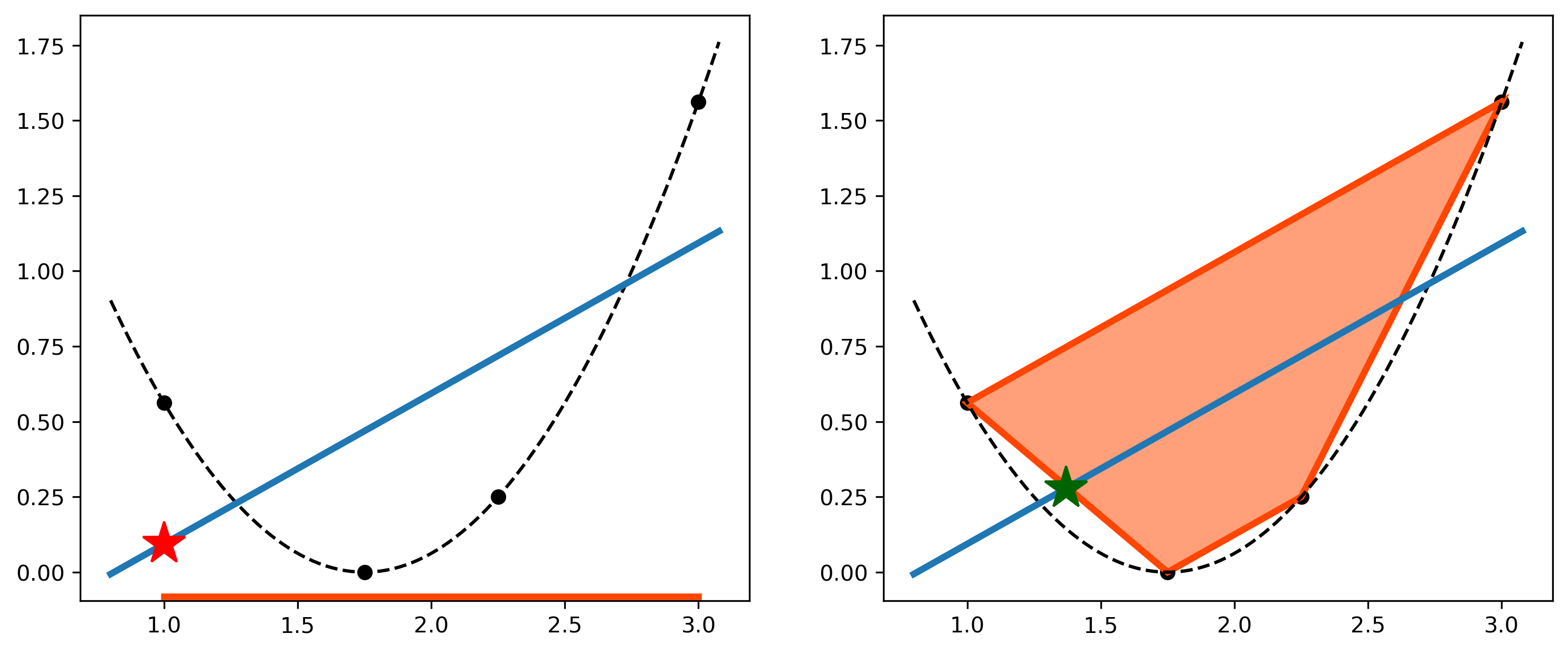
Figure 1: Illustration of $\operatorname{CH}$ on the left and $\operatorname{CH}^{+}$ on the right. $\operatorname{CH}^{+}$ exhibits better function-value and optimal-solution errors.

4 Numerical Results

To evaluate the extended validity domain $\operatorname{CH}^{+}$ introduced in Section 3, we adopt a procedure introduced by Shi et al. (2022). To this end, in the following subsections, we define the concept of a basic experiment, then describe our method for generating multiple experiments, and finally detail the optimization results. All numerical experiments were coded using Python 3.10.8 and Gurobi 11.0 and conducted on a single Xeon E5-2680v4 core running at 2.4 GHz with 8 GB of memory under the CentOS Linux operating system. The code and results are publicly shared at https://github.com/yillzhu/extvdom.

4.1 Definition of an experiment

In our testing, we define an experiment to be the full specification of six design options:

• Ground truth, i.e., a true optimization problem of the form $v^{*}=\min_{x}\left\{f(x):x\in X\right\}$ for which the function $f(x)$ and the true optimal value $v^{*}$ are known. A true optimal solution $x^{*}\in\text{Opt}^{*}$ is known as well. This corresponds to the simplified optimization (4) discussed in Section 2.1 in which the learned function lies in the objective, not the constraints. We will interchangeably identify a ground truth with its function $f$.

• Sampling rule, i.e., a rule ${\cal R}$ describing how to sample points in $X$.

• Sample size, i.e., the number of points $N$ to sample in $X$.

• Noise level, i.e., a scale factor $\sigma$ corresponding to the amount of random noise added to the function evaluations of $f$ during sampling.

• Seed, i.e., the seed $s$ used to initiate the random number generator before sampling.

• ML technique, i.e., the machine-learning technique ${\cal M}$ used to learn $\hat{f}$ from noisy evaluations of $f$.

Once the ground truth $f$, sampling rule ${\cal R}$, sample size $N$, noise factor $\sigma$, seed $s$, and ML model ${\cal M}$ are specified, an experiment proceeds as follows. Setting the seed $s$, we randomly sample $D_{N}\subseteq X$ following the sampling rule ${\cal R}$, and then we evaluate $f$ at all points in $D_{N}$ adding random noise scaled by the noise factor $\sigma$. Then we use the ML technique ${\cal M}$ to learn the approximation $\hat{f}$ using the empirical data $D_{N}$ and the noisy function values $f(D_{N})$. The experiment continues by solving (4) based on $\hat{f}$ with an additional validity-domain constraint for several different domains.

In short, an experiment specifies the six design options, builds the optimization model based on $\hat{f}$, and solves the model multiple times, each time testing a different validity domain. Because the ground truth is known, the errors defined in Section 2.2 are easily computed for each validity domain. This allows us to determine, for a given experiment, which validity domain yields smaller errors. Finally, by aggregating these errors over multiple experiments, we can identify trends in the performance of different validity domains.

4.2 Generating multiple experiments

Following Shi et al. (2022), we test seven different ground truths corresponding to seven challenging nonlinear benchmark functions from the literature (see, for example, Surjanovic and Bingham (2023)), namely $f\in\left\{\text{\em Beale, Griewank, Peaks, Powell, Qing, Quintic, Rastrigin}\right\}.$ The input dimension $n_{1}$ of these functions varies from 2 to 10, and in each case, $X$ is an $n_{1}$-dimensional box. Further, we consider two sampling rules ${\cal R}\in\{\text{\em Uniform, Normal}\},$ where Uniform indicates a uniform sample over the box domain $X$ and Normal indicates a jointly independent normal sample around the global minimum $x^{*}\in X$ of $f$ with covariance matrix $\rho I$, where $I$ is identity matrix of size $n_{1}$ and $\rho$ is problem-specific. In particular, we choose $\rho$ to be $1/6$ of the distance of $x^{*}$ to the boundary of $X$. Due to the nature of the normal distribution in each dimension, this ensures samples $D_{N}$ that tend to be close to $x^{*}$ and highly unlikely to be outside $X$.

The sample size is taken as $N\in\bigl{\{}1000,2000,3000\bigr{\}}$, and the noise is a zero-mean univariate normal distribution with standard deviation equal to $\sigma$ times the standard deviation of the noisy $f(D_{N})$ function values, where the scale factor $\sigma\in\bigl{\{}0.0,0.1,0.2\bigr{\}}$. In particular, $\sigma=0.0$ corresponds to the no-noise case. Furthermore, we take 100 seeds, specifically $s\in\bigl{\{}2023,2024,\dots,2122\bigr{\}}$.

In addition, we test three different machine learning models ${\cal M}$ using the scikit-learn package of Python: ${\cal M}\in\left\{\text{\em RandomForestRegressor, GradientBoostingRegressor, MLPRegressor\/}\right\}.$ In particular, we implement RandomForestRegressor with 100 trees and maximum depth of 5; GradientBoostingRegressor with 100 boosting stages and a maximum depth of 5 for the individual regression estimators; and MLPRegressor with 2 hidden layers and 30 neurons in each layer. (For each experiment independently, we also tried using grid search on the parameters to find the best model for that experiment. Ultimately, we found that the overall conclusions about the various validity domains in Section 4.3 were very similar. So we have fixed the parameters of ${\cal M}$ to simplify our experiments and reduce testing time.) Before constructing the ML models, the input features are standardized in $[0,1]$ using min-max scaling, and the noisy function values are normalized to mean 0 and standard deviation 1.

We generate experiments by looping over all combinations of $(f,{\cal R},N,\sigma,s,{\cal M})$ for a total of $7\times 2\times 3\times 3\times 100\times 3=37,800$ experiments. To provide a snapshot of the quality of the ML models, as well as the time required to compute them, Table 1 shows the average $R^{2}$ scores broken down by ground truth and ML technique, and similarly Table 2 shows the median training times (in seconds). Specifically, for the calculation of each $R^{2}$ value, we train and test the model using an 80-20 split of the data. However, the models used for optimization as described in the next subsection are trained on the complete data set.

	Beale	Griewank	Peaks	Powell	Qing	Quintic	Rastrigin
RandomForestRegressor	0.88	0.34	0.87	0.55	0.66	0.82	0.17
GradientBoostingRegressor	0.90	0.39	0.97	0.83	0.89	0.92	0.42
MLPRegressor	0.93	0.62	0.90	0.91	0.89	0.95	0.04

Table 1: Mean $R^{2}$ scores over all 37,800 experiments, grouped by function and ML technique.

	Beale	Griewank	Peaks	Powell	Qing	Quintic	Rastrigin
RandomForestRegressor	0.35	0.46	0.34	0.47	0.65	0.50	0.75
GradientBoostingRegressor	0.24	0.41	0.24	0.41	0.72	0.49	0.89
MLPRegressor	2.42	1.75	1.64	1.76	1.55	1.23	2.19

Table 2: Median training times (in seconds) over all 37,800 experiments, grouped by function and ML technique.

4.3 Optimization results

For each experiment, we solve the corresponding optimization model four times by varying the validity domain $V\in\left\{\text{{\sc Box}, CH, {\sc IsoFor}, CH${}^{+}$}\right\},$ where Box, CH, and CH⁺ are defined in Sections 2–3, and IsoFor refers to the isolation-forest validity domain of Shi et al. (2022), which has also been described in Section 2. For IsoFor, we follow Shi et al. (2022) by setting hyperparameters to their default values and by taking the maximum depth of a tree to be 5 for the Beale and Peaks functions and 6 otherwise. Tables 3 and 4 show the median setup and solve times for all combinations of ML technique and validity domains. By setup time, we mean the time required to build and pass the optimization to Gurobi, including the constraint which sets $y$ equal to the output of the learned function $\hat{h}(x)$, where $\hat{h}$ has already been trained and stored in memory. Although computation times are not the main focus in this paper, we see that IsoFor requires more time in general, while $\operatorname{CH}^{+}$ can take between 1-4 times as long as Box and $\operatorname{CH}$.

	Box	$\operatorname{CH}$	IsoFor	$\operatorname{CH}^{+}$
RandomForestRegressor	1.23	1.23	41.25	1.23
GradientBoostingRegressor	1.28	1.27	41.47	1.27
MLPRegressor	0.01	0.02	40.47	0.02

Table 3: Median optimization setup times (in seconds) over all 37,800 experiments, grouped by ML technique and validity domain.

	Box	$\operatorname{CH}$	IsoFor	$\operatorname{CH}^{+}$
RandomForestRegressor	0.86	1.31	3.56	1.48
GradientBoostingRegressor	5.40	6.70	14.35	14.76
MLPRegressor	0.09	0.23	24.24	0.39

Table 4: Median optimization solve times (in seconds) over all 37,800 experiments, grouped by ML technique and validity domain.

We now examine the errors associated with each validity domain. Table 5 presents results for all experiments grouped by function, type of error, and sampling rule. Each group then has four errors corresponding to the four validity domains. Furthermore, within each group of four errors, we scale so that the median error corresponding to Box equals 1.00, thus facilitating comparison of the different validity domains.

Function	Validity Domain	Median Function Value Error		Median Optimal Value Error		Median Optimal Solution Error
		Uniform	Normal	Uniform	Normal	Uniform	Normal
Beale	Box	1.00	1.00	1.00	1.00	1.00	1.00
	$\operatorname{CH}$	0.97	0.87	1.00	0.97	1.01	1.18
	IsoFor	0.63	0.76	0.73	0.91	0.81	0.52
	$\operatorname{CH}^{+}$	0.09	0.35	0.16	0.72	0.86	0.79
Griewank	Box	1.00	1.00	1.00	1.00	1.00	1.00
	$\operatorname{CH}$	0.73	0.95	1.09	1.00	0.92	0.97
	IsoFor	0.86	1.00	1.56	1.00	0.21	0.90
	$\operatorname{CH}^{+}$	0.49	0.53	1.18	0.90	0.89	1.08
Peaks	Box	1.00	1.00	1.00	1.00	1.00	1.00
	$\operatorname{CH}$	1.00	1.00	1.00	1.00	1.01	1.01
	IsoFor	1.47	1.25	1.16	1.01	1.04	0.88
	$\operatorname{CH}^{+}$	1.02	0.68	1.00	0.94	0.93	0.92
Powell	Box	1.00	1.00	1.00	1.00	1.00	1.00
	$\operatorname{CH}$	0.99	1.03	0.98	0.91	0.95	0.95
	IsoFor	0.90	1.06	0.89	0.79	0.66	0.59
	$\operatorname{CH}^{+}$	0.09	0.17	0.15	0.23	0.78	0.63
Qing	Box	1.00	1.00	1.00	1.00	1.00	1.00
	$\operatorname{CH}$	0.61	0.54	1.00	1.00	0.83	0.83
	IsoFor	1.20	0.73	1.00	1.00	0.75	0.72
	$\operatorname{CH}^{+}$	0.41	0.45	0.79	0.95	0.70	0.54
Quintic	Box	1.00	1.00	1.00	1.00	1.00	1.00
	$\operatorname{CH}$	0.63	0.42	0.90	0.36	0.97	0.97
	IsoFor	0.25	0.16	0.94	0.26	0.77	0.75
	$\operatorname{CH}^{+}$	0.13	0.06	1.00	0.25	0.92	0.74
Rastrigin	Box	1.00	1.00	1.00	1.00	1.00	1.00
	$\operatorname{CH}$	0.87	0.66	1.02	1.49	0.88	0.65
	IsoFor	0.92	0.84	1.04	1.39	0.82	0.63
	$\operatorname{CH}^{+}$	0.68	0.49	1.13	1.54	0.70	0.63

Table 5: Errors for all 37,800 experiments, grouped by function, type of error, and sampling rule. In each group of four errors corresponding to the four validity domains, the errors are scaled so that Box has value 1.00 in order to facilitate comparison among the different validity domains.

For both sampling rules, we see small function value errors for $\operatorname{CH}^{+}$. In particular, for six of the seven functions, $\operatorname{CH}^{+}$ achieves the best median function value error for Uniform. For the seventh function (Peaks), $\operatorname{CH}^{+}$ achieves nearly the best—1.02 versus 1.00 for both Box and $\operatorname{CH}$. For the Normal sampling rule, $\operatorname{CH}^{+}$ also performs well, where it achieves the best median function value error for all seven functions.

For the optimal value and optimal solution errors, $\operatorname{CH}^{+}$ performs competitively. With respect to Uniform, for five of the seven functions, $\operatorname{CH}^{+}$ has either the best median optimal value error or the best median optimal solution error. For Normal, we see this performance for all seven functions.

In Figure 2, we examine more closely the behavior of the function value error of $\operatorname{CH}^{+}$ compared to that of $\operatorname{CH}$ over all experiments. We plot the empirical distribution of the ratio of the function value error for $\operatorname{CH}^{+}$ divided by the function value error for $\operatorname{CH}$. When the ratio is less than 1.0 for a given experiment, $\operatorname{CH}^{+}$ has a better function value error; when the ratio is greater than 1.0, $\operatorname{CH}^{+}$ has a worse error on that experiment. In Figure 2, the distribution of ratios is plotted on a logarithmic scale, and two additional pieces of information are shown. First, a vertical dotted line is plotted to mark the ratio 1.0. Second, the percentage of experiments to the left of 1.0, i.e., when $\operatorname{CH}^{+}$ is performing better, is annotated. We see in particular that $\operatorname{CH}^{+}$ achieves a better function value error than $\operatorname{CH}$ on over 55% of experiments. In addition, the left tail of the distributions show that $\operatorname{CH}^{+}$ can reduce the error by up to a factor of 1,000, whereas the right tail indicates that the error from $\operatorname{CH}^{+}$ is usually no more than 100 times the error from $\operatorname{CH}$. Finally, we note that in both panels of Figure 2, the mode is 1.0, indicating that the most common situation is for $\operatorname{CH}^{+}$ and $\operatorname{CH}$ to yield the same function value error. Analogous plots comparing the function value error of $\operatorname{CH}^{+}$ compared to that of Box and respectively IsoFor show similar results.

Figure 2: Empirical distributions of the ratio of the function value error of $\operatorname{CH}^{+}$ divided by the function value error of $\operatorname{CH}$, grouped by sampling rule.

5 Two Stylized Optimization Models

In this section, we examine the performance of our extended validity domain $\operatorname{CH}^{+}$ in the context of two stylized optimization problems. In both cases, we see that $\operatorname{CH}^{+}$ more effectively manages the function value and feasibility errors.

5.1 A simple nonlinear optimization

Consider the true optimization problem $v^{*}:=\min_{x\in\mathbb{R}^{n_{1}}}\left\{c^{T}x:\|x\|\leq 1,x\in[-1,1]^{n_{1}}\right\}$ where $c\in\mathbb{R}^{n_{1}}$ is an arbitrary vector satisfying $\|c\|=1$. It is easy to see that $v^{*}=-1$ and the unique optimal solution is $x^{*}=-c$. This is an instance of (2) with $f(x):=c^{T}x$, $X:=[-1,1]^{n_{1}}$, $g$ nonexistent, $\theta(y):=y-1$, and $h(x):=\|x\|$. In this subsection, we will consider small values of $n_{1}$, specifically $n_{1}\in\{5,10\}$.

We conduct a single experiment by randomly generating $c$ uniformly on the surface of the Euclidean unit ball, sampling $N=1,000$ points $x$ such that the Euclidean norm of $x$ is uniform in $[0.5,1.5]$, and evaluating $h(x)+0.05\epsilon$ on all samples, where $\epsilon$ is a standard normal random variable. We train the function $\hat{h}$ using the Python function MLPRegressor just as in Section 4 using the same hyperparameter choices.

For a single experiment, we then test the validity domains Box, $\operatorname{CH}$, and $\operatorname{CH}^{+}$. In particular, $\operatorname{CH}^{+}$ is constructed as the convex hull of $F_{N}^{+}$ according to (10), where $F_{N}^{+}$ is the set of feasible samples in the full extended space defined by (9). Despite the fact that the evaluations of $h$ are noisy, we include a point $x$ in $F_{N}^{+}$ if $\|x\|+0.05\epsilon\leq 1$, where $\epsilon$ is the added noise. In particular, the noise affects the construction of the set $F_{N}^{+}$. Because $x$ has been sampled with radius uniform in $[0.5,1.5]$, the expected cardinality of $F_{N}^{+}$ is approximately $N/2$.

For $n_{1}=5$, we run 100 experiments and show the median errors in Table 6, and then we repeat the same experiments for $n_{1}=10$. Similar to Table 5 in Section 4, we collect the results in Table 6, grouped by $n_{1}$. For each sub-grouping of three errors, we scale such that Box has error 1.0. We see clearly that $\operatorname{CH}^{+}$ achieves the same or better median function value error and significantly better median feasibility error (in fact zero to two decimal places).

$n_{1}$	Validity Domain	Median Function Value Error	Median Optimal Value Error	Median Optimal Solution Error	Median Feasibility Error
5	Box	1.00	1.00	1.00	1.00
	CH	0.99	0.94	0.94	0.99
	$\operatorname{CH}^{+}$	0.48	2.32	1.04	0.00
10	Box	1.00	1.00	1.00	1.00
	CH	0.17	0.13	0.48	0.17
	$\operatorname{CH}^{+}$	0.18	1.19	0.68	0.00

Table 6: Median errors of Box, $\operatorname{CH}$, $\operatorname{CH}^{+}$ methods in the stylized simple nonlinear optimization model, grouped by dimension $n_{1}$. The median is taken over 100 experiments, and each column is scaled so that Box has error $1.00$ in each column.

Since $\operatorname{CH}^{+}$ has been constructed as the convex hull of $F_{N}^{+}$, which includes only feasible samples—and since the true feasible set is convex—it is perhaps not surprising that $\operatorname{CH}^{+}$ achieves the smallest feasibility error. So we repeated the same tests but for the case when $\operatorname{CH}^{+}$ is the convex hull of $D_{N}^{+}$ defined in (8), i.e., both feasible and infeasible sample points are included. The corresponding median feasibility errors were 0.08 and 0.00, respectively, indicating that feasibility is also managed well in this case.

5.2 A price optimization

We also test $\operatorname{CH}^{+}$ on a stylized price optimization problem, which is a preview of the case study in Section 6. Imagine a company with two substitute products, labeled as products 1 and 2. Product 1 is the low-price product, and product 2 is the high-price product. Demands $d_{1}$ and $d_{2}$ for the respective products are functions of their prices, $p_{1}$ and $p_{2}$. The company would like to set prices so as to maximize revenue under various constraints. The true model is:

$$\max_{p_{1},p_{2}}\quad d_{1}p_{1}+d_{2}p_{2}$$ (11a)

$$\operatorname{s.t.}\quad\ p_{1}\in[6.5,9.5]\quad p_{2}\in[7.5,10.5]\quad p_{1}+0.5\leq p_{2}\leq p_{1}+1.5$$ (11b)

$$d_{1}=10^{7}p_{1}^{-3.2}p_{2}^{0.5}\quad d_{2}=10^{7}p_{1}^{1.5}p_{2}^{-2.2}\quad d_{1}+d_{2}\leq 1.8\times 10^{6}.$$ (11c)

Here, the objective function (11a) is the total revenue of the company; constraint (11b) describes the allowable prices; and constraint (11c) describes the demand functions for products 1 and 2 as well as a cap on demand corresponding what can actually can be sold. Gurobi solves this problem, reporting a true optimal solution of $(p_{1}^{*},p_{2}^{*})=(9.50,10.31)$. At optimality, the demand constraint is active.

To perform numerical tests, we replace the demand functions with learned models and enforce different validity-domain constraints. To learn the demand functions, we uniformly sampled 1,000 points in the box domain of $(p_{1},p_{2})$, evaluated the corresponding $(d_{1},d_{2})$ without noise, and learned the approximation $(\hat{d}_{1},\hat{d}_{2})$ using a simple quadratic regression. (Note that if the data had been learned with a log-log regression, then the learned model would be exact.) We tested Box, $\operatorname{CH}$, and $\operatorname{CH}^{+}$. The convex hull used for $\operatorname{CH}$ is taken over the 2-dimensional samples $(p_{1},p_{2})$, while our extended convex hull $\operatorname{CH}^{+}$ is taken over the 4-dimensional samples $(p_{1},p_{2},d_{1},d_{2})$. The median errors of the validity domains are summarized in Table 7, where as before we scale the Box errors to 1.00. We see clearly that $\operatorname{CH}^{+}$ achieves much lower function value and feasibility errors than either Box or $\operatorname{CH}$, although the optimal value and optimal solution errors are notably higher. We believe that overall this constitutes an advantage of $\operatorname{CH}^{+}$ because, generally speaking, one cannot have true optimality without true feasibility.

	Median Function Value Error	Median Optimal Value Error	Median Optimal Solution Error	Median Feasibility Error
Box	1.00	1.00	1.00	1.00
CH	0.99	1.06	1.06	0.99
$\operatorname{CH}^{+}$	0.16	10.82	16.92	0.11

Table 7: Median errors of Box, $\operatorname{CH}$, and $\operatorname{CH}^{+}$ in the price optimization model. The median is taken over 10,000 experiments, and each sub-grouping of three errors is scaled so that Box has error $1.00$.

6 A Case Study

In this section, we investigate an avocado-price optimization model recently described by Gurobi Optimization, the makers of Gurobi (2023). The goal is to set the prices and supply quantities for avocados across eight regions of the United States while incorporating transportation and other costs and maximizing the total national profit from avocado sales. A critical component of the model is the relationship between avocado prices and the demand for avocados in each region. Gurobi Optimization proposed to learn the demand function using ML techniques based on observed sales data. Then the demand function could be embedded in the optimization model, thus creating a case study for constraint learning (CL). We revisit this study in light of our extended validity domain $\operatorname{CH}^{+}$ proposed in Section 3.

Note that, in this case study, there is no ground truth, and so we are unable to measure the errors defined in Section 2.2. Instead, we seek experimental insights from this case.

6.1 Avocado price model

The eight regions are indexed by $r\in\{1,\ldots,8\}$, and the total units of avocado imported into a single port in the United States is denoted by $B$. The per-unit cost of waste is $\alpha$, which is independent of the region, and the transportation cost from the port to region $r$ is $\beta_{r}$. The learned demand function for avocados in region $r$ at sales price $p$ is denoted $\hat{d}(p,r)$. The optimization variables are the unit price $p_{r}$ and units supplied $x_{r}$ for region $r\in\{1,\ldots,8\}$. Auxiliary variables $s_{r}$ and $w_{r}$ represent the units sold and units wasted per region, respectively. The model formulation is

$$\max\quad \sum_{r=1}^{8}\left(p_{r}s_{r}-\alpha\,w_{r}-\beta_{r}x_{r}\right)$$ (12a)

$$\operatorname{s.t.}\quad\, \sum_{r=1}^{8}x_{i}=B$$ (12b)

$$s_{r}\leq\min\{x_{r},\hat{d}(p_{r},r)\}\quad w_{r}=x_{r}-s_{r}\quad p_{r}\geq 0,\ x_{r}\geq 0\quad\forall\ r\in\{1,\cdots,8\}.$$ (12c)

The nonconvex, bilinear objective (12a) calculates profit by subtracting the cost of shipping and waste from the revenue over all regions. Constraint (12b) ensures that the total units supplied equals the import quantity, and constraint (12c): defines the number of units sold in a region to be no larger than the minimum of supply and predicted demand in the region; sets the number of units wasted to be the difference between number of units supplied and the number sold; and finally enforces nonnegativity of $p_{r}$ and $x_{r}$. In practice, there may also be upper bounds on $p_{r}$ and $x_{r}$.

6.2 Dataset and predictive model

The dataset to learn $\hat{d}(p,r)$ has been prepared by Gurobi Optimization from two sources, and the combined dataset is hosted at Gurobi Optimization’s GitHub account. One source is the Hass Avocado Board (HAB), from which Gurobi Optimization has retrieved data for the years 2019 to 2022, and the second source is Kaggle, which hosts data originating from HAB for the years 2015 to 2018. The total time span of the data is thus from 2015 to 2022. Note that, since true demand is not observed directly, sales data is used instead as the best available proxy of demand, and we do not consider other issues such as non-stationarity of demand over time.

The data has been cleaned and processed such that each observation includes a date (indicating the start of a calendar week), a seasonality indicator for that specific week (corresponding to $1$ for peak and 0 for off-peak), the region, the number of units of avocados sold (in millions of units), and the average price per unit. For this data set, the average units sold over all observations is 3.9 million, the average price is $1.14, and the average revenue is $4.23 million; these values describe a typical week in a typical region. Aggregating up to the entire United States, in a typical week, the average units sold is 31.0 million at an average price of $1.14 for an average revenue of $33.85 million. Restricting to just off-peak data, in a typical off-peak week, the average units sold across the U.S. is 28.6 million at an average price of $1.14 for an average revenue of $31.10 million.

Following Gurobi Optimization’s example, we use a gradient boosting regressor implemented using the Python’s scikit-learn package to learn the demand function $\hat{d}(p,r)$ based on four features of the data: year (not the specific week), the seasonality indicator, region, and price. For convenience, we label these features Year, Peak, Region, and Price, respectively. The label for the response variable in the data is Units Sold.

Figure 3: Avocado data (light blue dots), predicted demand function (orange curve), and four optimal solutions. The default (i.e., no validity domain) is dark blue, Box is dark green, $\operatorname{CH}$ is dark orange, and $\operatorname{CH}^{+}$ is dark red.

Figure 3 depicts eight panels, one for each region in the data. Here, the regions are labeled with their descriptive names, e.g., Northeast and Plains, as opposed to their index numbers $r\in\{1,\ldots,8\}$. Each panel depicts a scatter plot of light-blue dots, which show the observed data, where the horizontal axis is Price and the vertical axis is Units Sold (in millions). We note that each panel is plotted over the region $0.6\leq p_{r}\leq 2.0$, representing a unit price between $0.60 and $2.00 for all regions. In addition, in each panel the learned function $\hat{d}(p_{r},r)$ with fixed values Year $=2023$ and Peak = $0$ is plotted as an orange curve through the data; the vertical axis is labeled as Predicted Demand. (Each panel also contains additional information in the form of four additional colored dots, which we explain in the next subsection.) We observe the expected inverse relationship between price and demand. Further, the fitted demand function does a reasonably good job capturing the relationship between price and demand in each of the eight regions.

6.3 Effect of validity domains

We now solve (12) for various validity domains. All experiments are executed using Gurobi 11.0 as the optimization solver. In these optimizations, we fix Year $=2023$, i.e., predicting into the next year beyond the data, and we also fix Peak $=0$. Hence, we are optimizing prices for a single off-peak week in 2023. We set the remaining model parameters as Gurobi Optimization has done with $B=30$, $\alpha=0.1$, and the following transportation coefficients $\beta_{r}$: Great Lakes = 0.3, Midsouth = 0.1, Northeast = 0.4, Northern New England = 0.5, South Central = 0.3, Southeast = 0.2, West = 0.2, and Plains = 0.2. Because Gurobi was not able to solve all instances to the default optimality tolerance in a reasonably small amount of time, we set a time limit of 600 seconds (10 minutes) and report the best feasible value found.

When (12) is optimized with a uniform upper bound of $p_{r}\leq 2.0$ for all regions, the optimal value is $45.84 million. A corresponding best solution is depicted with dark-blue dots in the panels of Figure 3. In particular, for all but the Northern New England region, the best solution sets $p_{r}=2.0$, i.e., the price is at the upper bound of $2.00. Particularly striking is that the solution is visually quite far from the observed data. One may ask if this solution is trustworthy given that the demand predictions are likely to be less reliable away from the observed data.

We next test the three validity domains Box, CH, and CH⁺ with the caveat that all validity domains are considered with respect to the prices $p$ but not the shipped quantities $x$ because the historical data on $x$ are not available. Our hope is that these validity domains can help alleviate the uncertainty inherent in the default solution just mentioned. We would also like to compare and contrast these three validity domains in this setting. Our observations are summarized as follows:

• Box: For each $r$ independently, we constrain $p_{r}$ to be within its observed minimum and maximum values; see (6). The best reported value is $39.51 million, and the corresponding prices per region are shown in Figure 3 as orange dots. Compared to the blue dots of the default solution, the orange dots are “pulled back” much closer to the data. It is clear that Box does not allow as much extrapolation in the optimal solution, and hence one can expect the predicted demand to be more accurate. Hence, one can expect the final profit number to be more reliable.

• CH: This validity domain is defined to be the convex hull in $\mathbb{R}^{8}$ of the 8-tuples $(p^{(i)}_{1},\ldots,p^{(i)}_{8})$, where $i=1,\ldots,N$ indexes over all observations; see (7). The value is $38.02 million, and Figure 3 shows the prices as green dots. As with Box, the prices are visually closer to observed price data, and hence one can expect the overall optimization result to be more reliable.

• $\operatorname{CH}^{+}$: Finally, we consider our extended validity domain, which enforces that the concatenated variables and demand predictions $(p_{1},\ldots,p_{8},\hat{d}(p_{1},1),\ldots,\hat{d}(p_{8},8))$ lie in the convex hull of the observed data $(p^{(i)}_{1},\ldots,p^{(i)}_{8},d^{(i)}_{1},\ldots,d^{(i)}_{8})$ where $i=1,\ldots,N$; see (10). This convex hull lies in $\mathbb{R}^{16}$. The optimized prices are shown as red dots in Figure 3, and the value is $32.54 million. Although this value is significantly less than the preceding objective values (compare to the value of $38.02 for $\operatorname{CH}$, for example), the position of the red dots is considerably closer to the original data set. In fact, based on the two-dimensional panels in Figure 3, it appears that the optimal prices are actually embedded inside the data, although this may be a visual artifact of the projection of a 16-dimensional image down to eight individual 2-dimensional scatter plots. In any case, one can expect that the predictions $\hat{d}(p,r)$ are the most reliable for this validity domain, making the overall optimization more reliable.

As a final comment, we recall that the empirical data shows an average revenue of $31.10 million in a typical off-peak week; see the discussion in Section 6.2. The final optimal value of $32.54 million for $\operatorname{CH}^{+}$ is certainly in line with this empirical average and constitutes an increase of 4.6%.

7 Conclusions

We have studied the use of validity domains to reduce the errors associated with the constraint-learning (CL) framework. Based on the intuition of using the convex hull to learn both the data set and the optimization problem itself, we have proposed a new extended validity domain, called $\operatorname{CH}^{+}$. Our numerical studies have shown that $\operatorname{CH}^{+}$, compared to other common methods in the literature, is competitive in terms of computational effort and tends especially to reduce the function value and feasibility errors. Beyond stylized numerical results, the avocado case study has shown the applicability and adaptability of our approach to real-world situations.

We mention some opportunities for future research. First, the model (1) based on $\hat{h}$ may be infeasible in general, and when validity domains such as $\operatorname{CH}$ or $\operatorname{CH}^{+}$ are also enforced, infeasibility will be, in a sense, even more likely. It will be interesting to investigate the underlying properties that make (1) feasible, to understand when $\operatorname{CH}^{+}$ maintains this feasibility, and if not, then to develop alternate validity domains that do maintain it. Second, we have used the convex hull in an extended space in part because $\operatorname{CH}$ in the original space is well-studied and possesses good properties. Of course, there exist other techniques for creating validity domains in the original space as described in Section 2. One future idea to explore is whether these other techniques, similar to $\operatorname{CH}^{+}$, can also be effective in the extended space.

References

- Bengio et al. [2021] Yoshua Bengio, Andrea Lodi, and Antoine Prouvost. Machine learning for combinatorial optimization: a methodological tour d’horizon. European Journal of Operational Research, 290(2):405–421, 2021.
- Bergman et al. [2022] David Bergman, Teng Huang, Philip Brooks, Andrea Lodi, and Arvind U. Raghunathan. JANOS: an integrated predictive and prescriptive modeling framework. INFORMS J. Comput., 34(2):807–816, 2022. ISSN 1091-9856,1526-5528. doi: 10.1287/ijoc.2020.1023. URL https://doi.org/10.1287/ijoc.2020.1023.
- Ceccon et al. [2022] Francesco Ceccon, Jordan Jalving, Joshua Haddad, Alexander Thebelt, Calvin Tsay, Carl D. Laird, and Ruth Misener. OMLT: optimization & machine learning toolkit. J. Mach. Learn. Res., 23:Paper No. [349], 8, 2022. ISSN 1532-4435,1533-7928.
- Courrieu [1994] Pierre Courrieu. Three algorithms for estimating the domain of validity of feedforward neural networks. Neural Networks, 7(1):169–174, 1994.
- De Filippo et al. [2018] Allegra De Filippo, Michele Lombardi, and Michela Milano. Methods for off-line/on-line optimization under uncertainty. In Proceedings of the Twenty-Seventh International Joint Conference on Artificial Intelligence, IJCAI-2018. International Joint Conferences on Artificial Intelligence Organization, July 2018. doi: 10.24963/ijcai.2018/177. URL http://dx.doi.org/10.24963/ijcai.2018/177.
- Fajemisin et al. [2023] Adejuyigbe O Fajemisin, Donato Maragno, and Dick den Hertog. Optimization with constraint learning: a framework and survey. European Journal of Operational Research, 2023.
- Gurobi [2023] Gurobi. Gurobi Optimizer Reference Manual, 2023. URL https://www.gurobi.com.
- Kotary et al. [2021] James Kotary, Ferdinando Fioretto, Pascal Van Hentenryck, and Bryan Wilder. End-to-end constrained optimization learning: A survey, 2021.
- Liu et al. [2008] Fei Tony Liu, Kai Ming Ting, and Zhi-Hua Zhou. Isolation forest. In 2008 eighth ieee international conference on data mining, pages 413–422. IEEE, 2008.
- Maragno et al. [2023] Donato Maragno, Holly Wiberg, Dimitris Bertsimas, S. Ilker Birbil, Dick den Hertog, and Adejuyigbe Fajemisin. Mixed-integer optimization with constraint learning, 2023.
- Mistry et al. [2019] Miten Mistry, Dimitrios Letsios, Gerhard Krennrich, Robert M. Lee, and Ruth Misener. Mixed-integer convex nonlinear optimization with gradient-boosted trees embedded, 2019.
- Sadana et al. [2024] Utsav Sadana, Abhilash Chenreddy, Erick Delage, Alexandre Forel, Emma Frejinger, and Thibaut Vidal. A survey of contextual optimization methods for decision making under uncertainty, 2024.