Lasso Multinomial Performance Indicators for in-play Basketball Data

Abstract

A typical approach to quantify the contribution of each player in basketball uses the plus/minus approach. Such plus/minus ratings are estimated using simple regression models and their regularised variants with response variable either the points scored or the point differences. To capture more precisely the effect of each player and the combined effects of specific lineups, more detailed possession-based play-by-play data are needed. This is the direction we take in this article, in which we investigate the performance of regularized adjusted plus/minus (RAPM) indicators estimated by different regularized models having as a response the number of points scored in each possession. Therefore, we use possession play-by-play data from all NBA games for the season 2021-22 (322,852 possessions). We initially present simple regression model-based indices starting from the implementation of ridge regression which is the standard technique in the relevant literature. We proceed with the lasso approach which has specific advantages and better performance than ridge regression when compared with selected objective validation criteria. Then, we implement regularized binary and multinomial logistic regression models to obtain more accurate performance indicators since the response is a discrete variable taking values mainly from zero to three. Our final proposal is an improved RAPM measure which is based on the expected points of a multinomial logistic regression model where each player’s contribution is weighted by his participation in the team’s possessions. The proposed indicator, called weighted expected points (wEPTS), outperforms all other RAPM measures we investigate in this study.

Keywords: plus/minus, RAPM, regularization, logistic regression, expected points (EPTS)

1 Introduction

Managing the workload of players is a complex process that challenges basketball coaches and analysts worldwide. This is one of the factors that account for the popularity of players’ evaluation criteria. Particularly in team sports, one of the most relevant and valuable metrics is the impact a player has on the outcome of his team. As the renowned Dean Oliver stated “Teamwork is the element of basketball most difficult to capture in any quantitative sense” [7].

A common way to assess the performance of teams and players is to use plus/minus indices. WINVAL is a software system that implements the adjusted plus/minus technique for basketball, which was created by Wayne Winston and Jeff Sagarin in 2002 [11]. It calculates the average point difference for each NBA player’s team per possession when the player is on the court. This number indicates how well the player’s team performed when he was playing. However, this technique has a major flaw: it favors players who often play with good teammates or against weak opponents. These players tend to appear more effective than they actually are.

Using only the information on the players’ teammates and opponents on the court, [9] and, later, [5, 6] suggested a ridge regression approach to measure the players’ contribution. The index was named Regularized Adjusted Plus/Minus (RAPM). The model has become popular and it was widely used in players’ performance analysis because of its benefits: i) it produces low-variance estimates; ii) it provides an evaluation metric for all players; iii) it provides more stable evaluation metrics for players that frequently play together because it handles multicollinearity in the fitted model; and iv) it allows easy interpretation of the RAPM evaluation metrics via the underlying fitted linear regression.

In this work, we study the performance of several approaches for the players’ evaluation of their offensive and defensive contributions using play-by-play NBA data. Each data observation (row in our dataset) refers to an offence (or equivalently possession). The response variable of interest is the outcome (i.e. achieved score) per possession that ranges from zero to six. Someone may be surprised by this range since, in basketball, the natural outcomes are from zero to three points. The additional values (4–6) are rare and may occur only due to offensive goal fouls or technical fouls.

In our analysis, we use the ridge regression approach as a starting point. A common issue in such studies is the performance evaluation of low-time players, whose RAPMs are usually found to be very high indicating that they over-perform in comparison to their actual contribution. As a second step, we applied lasso regularization method instead of ridge for the normal regression model. This improved the results, as lasso distinguishes the better and worse players more reasonably and realistically than the ridge regression. Moreover, players with average or non-important RAPM are automatically set to zero from the lasso approach. We consider this as an advantage of lasso over ridge regression since we are usually interested for evaluating only the top-rated or efficient players — in some occasions, we may also be interested in identifying the worst or inefficient players. Nevertheless, someone may argue that estimating a RAPM evaluation metric for every player is more desirable. A major disadvantage of both of these approaches is the use of the normal distribution to model a discrete response (the outcome per possession). Clearly, the normal distribution is not suitable to stochastically model such a response and other alternatives should be found to build a more accurate and statistically correct model.

Hence, we extended the standard ridge regression approach by using binary and multinomial logistic regression models. We first simplified the problem by using a regularized binomial model with a response of a binary variable indicating whether the offensive team scored or not. Surprisingly, the logistic regression RAPM estimates were found to be highly correlated with the usual RAPM values. In this way, we provide a different, valid interpretation for the usual normal regression-based RAPMs.

Finally, we produce a regularized multinomial logistic regression model for the points scored per possession. The model was fitted indirectly through three separate binomial models for the different types of points scored (one, two, and 3+). Here, a new evaluation metric is proposed based on the expected points per possession (EPTS) and its extended version, the weighted expected points (wEPTS). The latter index takes into consideration the proportion of possessions that each player participates in his team. It is derived as the points expected to be scored by the team over all games under the simplified scenario that all other players on court belong to the reference group with zero-lasso RAPM measures.

Our initial intuition that the multinomial model is more suitable for modelling the points per possession and for producing player evaluation metrics is confirmed since the obtained wEPTS evaluation index is found to be superior according to selected external validation criteria. Moreover, this metric seems to partially solve the problem related to the overestimation of the performance of low-time players. Another characteristic of the proposed regularized multinomial approach is that the overall EPTS (and wEPTS) index can be decomposed in three different RAPM measures, one for each possible scoring outcome (one, two and 3+). Therefore, the method can spot the best-performed players according to each scoring outcome. For example, some players might be more influential by participating in two-pointer offences and other players might participate more when their team scores a three-pointer. Our method will identify both of these types of players and account for their contribution. This is a unique characteristic of our approach that no other previously proposed method has.

The structure of the paper is as follows. Section 2 describes the data and the methodology used in this study. Section 3 presents the results of our analysis regarding RAPM and EPTS ratings and, in Section 4, we introduce the finally proposed weighted expected points (wEPTS) rating. Section 5 concludes with some interesting findings and discussions.

2 Material and Methods

2.1 Initial Raw Dataset

In this study, play-by-play possession NBA data were used from the 2021-2022 season. Data were collected from NBA logs. The data comprised of possessions as the study unit of analysis (i.e. observation) and the related information (features) of each possession, such as points scored and playing lineups of the two opponent teams. The original (unprocessed) dataset contained 322,852 observations (possessions) and 13 variables. A description of the available variables follows:

• home_off: A dichotomous variable that signifies whether the team in possession is the host or the visitor.

• pts: This is the main outcome variable which records the points achieved in each possession taking values ranging from zero to six (0–6). Naturally, the occurrence of five or six points in one possession was very rare. Hence, it was reasonable that there were only two and one possessions with five and six points, respectively.

• season_type: A dichotomous variable that shows the type of season the game occurred (regular season or playoffs).

• O1–O5 and D1–D5: String variables that refer to the players of the team in possession (i.e. in offence) and the opposing team (i.e. in defence), respectively, in each possession. Each string/character comprises by the team’s (abreviated) name & player’s name, e.g., LAC22 Ivica-Zubac.

2.2 Final Dataset

The original raw dataset was approrpiately transformed in order to be used in the subsequent analysis. Specifically, the players’-related variables (O1–O5 and D1–D5) were transformed into a series of dichotomous variables (one offensive and one defensive for each player who participated in at least one game of the NBA league). These dichotomous variables denote the presence or absence of each player in the field, in each possession, with the team in possession or the team in defence. For this dataset, we have considered a total of 717 players. Thus, the final data matrix is an $n\times m$ sparse matrix with $n=322,852$ rows (possessions) and $m=1,437$ columns with the features used in the analysis. The total set of features consists of $717\times 2$ binary variables used to evaluate the offensive and defensive contribution of each player (i.e. each player is split into their offensive and defensive coefficients) plus three extra columns from the original raw dataset: home_off (binary), season_type (factor with 2 levels), and pts (points per possession).

The number of points scored by the team in possession (pts) is the main outcome (or response) variable of this study. Therefore, the dichotomous variables $X^{o}_{j}$ of each player $j$ in the team in possession are coded as zero/one (0/1), while the corresponding variables $X_{j}^{d}$ of player $j$ in the defending team are coded as zero/minus one (0/-1); for $j\in\{1,2,\dots,K\}$ with $K$ denoting the total number of players in our dataset. This coding scheme reflects the positive and negative (or opposite) effect of each player on the outcome variable.

Concerning the outcome variable (pts), no points were scored in most of the possessions ($59.6\%$). Of the remaining ones, $26.2\%$ resulted in two points and $11.6\%$ in three points. One-point possessions accounted only for $2.5\%$ of the total number of possessions. This was due to the fact that two successful free throws (in one possession) were considered as two-point possessions. Finally, more than three points were scored in only $0.1\%$ of the possessions.

The number of possessions is almost balanced between the home and away teams, with a slight advantage for the away team (278 more possessions out of 322,852 total possessions). This is reasonable and expected due to the sequential nature of the game. Regarding the type of the game, most of the possessions ($93.2\%$) occurred in the regular season, as the NBA league format requires each team to play 82 games in the regular season and only 4–28 games in the playoffs.

2.3 Models and Analysis

In order to construct a player evaluation metric using statistical models, we require an efficiency measure as a dependent variable. Usually, in sports, this variable is the final outcome or score. For our study, which uses play-by-play data, the efficiency factor (or dependent or outcome variable) corresponds to the number of points scored by the offensive team in each possession.

In this section, we start from the standard approach in the Basketball bibliography for obtaining RAPM measures which is based on the normal regression model using ridge regression. The main drawback of such a model is that the normal distribution attached to it is incompatible with the use of the number of points scored in each possession as the dependent efficiency variable. Therefore, we proceed with models that are more suitable for this kind of response. Initially, we use a binomial logistic regression model with the binary indicator of scoring or not scoring per possession as a dependent efficiency variable. Although this model is more appropriate mathematically than the normal regression model, there is a loss of information since all different types of scoring are merged into one unified category. This loss of information (i.e. the different types of scores) is quite important for describing the nature of Basketball. For this reason, we proceed by proposing a multinomial regression logistic regression model which takes into consideration the three different outcomes of a possession. In all the above models, additionally to the ridge approach, we have also implemented lasso which has the characteristic that places specific players in an “average” category. Overall, lasso seems to outperform the ridge approach in many different perspectives that will be later explained in Section 3.

2.3.1 Low-time players

Prior to proceeding with the implemented models, we need to introduce the concept of Low-time players (LTPs). In the following, we use this term for the players who participate for less than a threshold of minutes per game, usually due to their restricted role in the team. Their performance may affect the evaluation metrics that are widely used to assess the contribution of basketball players to their teams’ success. For instance, conventional evaluation metrics do not take into consideration the context and quality of their playing time. Moreover, such metrics heavily depend on the performance of the other players on the court, as well as the quality of the opposing team. On this perspective, [4] argues that the quality and the performance of the team that a low-time player participates greatly affects their plus/minus ratings. As a result, poor players on good teams are overrated, while good players on poor teams are underrated.

A common way to resolve the problem is to impose a threshold on the playing time and exclude the corresponding LTPs from the calculation of the performance evaluation metrics; see for example in [9] and [6].

Subsequently, in the following, we consider as LTPs all players with playing time less than 200 minutes for the whole of the season. This threshold identifies 232 (out of 717) as LTPs which is the $32\%$ of the players in our dataset.

2.3.2 Linear normal regression with shrinkage methods

We first proceed with the standard approach which uses the normal regression model. Hence for considering $K=717$ different players, the model is written in the following way

$$Pts_{i}\sim N(\mu_{i},\sigma^{2})\mbox{~{}~{}with~{}~{}}\mu_{i}=b_{0}+\sum_{j=1}^{p}b_{j}X_{ij}+\sum_{k=1}^{K}\beta^{o}_{k}X_{ik}^{o}+\sum_{k=1}^{K}\beta^{d}_{k}X_{ik}^{d},$$ (1)

for $i=1,\dots,n$; where $n$ the total number of possessions in our dataset, $K$ is the total number of players under consideration, $Pts_{i}$ is the number of points achieved in possession $i$, $\mu_{i}$ is the expected points for possession $i$ for this model, $X_{ik}^{o}$ and $X_{ik}^{d}$ are the indicators of player $k$ in possession $i$ for the offensive and the defensive team, $X_{ij}$ refers to the extra covariate $j$ for possession $i$, $p$ is the number of extra covariates used in the model formulation, $\beta^{o}_{k}$ and $\beta^{d}_{k}$ are the offensive and defensive, respectively, RAPM coefficients for player $k$, $b_{k}$ are the effects of any extra covariates and $b_{0}$ is the overall constant of the model (usually referring to a reference average player obtained by players with zero or very close to zero RAPM coefficients). Finally, $\sigma^{2}$ is the error (or unexplained) variance which specifies the accuracy of the fitted model. In many published articles [see for example in 5, 6], the number of points per possession is multiplied by a factor of 100.

The additional covariates in the above formulation can be any data that enhance the forecasting of the final outcome of each possession. In our study, we used the following extra covariates: the home advantage of the team, the game type (regular season or playoff), and the teams involved in each game and possession. Nevertheless, none of these covariates were found to have a significant effect on the points in addition to the player’s RAPM coefficients. This result is consistent with the bibliography where they primarily focus on the estimation of RAPMs without introducing any additional information to the model; see, for example, in [5, 8].

Hence interest lies in the estimation of $\beta_{k}^{o}$ and $\beta_{k}^{d}$ coefficients (i.e. on ORAPM and DRAPM, respectively). The constant term $b_{0}$ here is a nuisance parameter with no direct or meaningful interpretation under the current formulation. The RAPM coefficients $\beta^{o}_{k}$ and $\beta^{d}_{k}$ measure the offensive and defensive, respectively, contribution of player $k$ for $k=1,\ldots,K$ players. Pairwise comparison between two players (denoted by $k$ and $m$) can be achieved by considering the RAPM differences $\beta^{o}_{k}-\beta^{o}_{m}$, $\forall k,m=1,\ldots,K,k\neq m$. These differences represent the mean discrepancy in the expected points scored by each player’s team when player $k$ substitutes player $m$ in a specific possession, with all other players on the court staying the same. Similarly, the difference between two defensive RAPMs $\beta^{d}_{k}-\beta^{d}_{m}$ ($\forall k,m=1,\ldots,K,k\neq m$) expresses the average discrepancy in points of each player’s team conceded (by the opponent team) when players $m$ plays instead of player $k$ with all other players on the court staying the same. Hence, the larger the difference is, the higher the offensive and defensive contribution of $k$ player.

Ridge Regression

The related literature mostly suggests ridge regression to derive RAPM ratings. Ridge regression shrinks coefficients towards zero but does not set them exactly equal to zero. This has the advantage that every player will get a non-zero evaluation coefficient for his offensive and defensive contributions; for more details about the ridge regression see [3] and in [9, 5, 4, 2] for the implementation in obtaining basketball RAPMs evaluation metrics.

In the implementation of ridge regression, for the estimation of RAPM coefficients, we have used 10-fold cross-validation in order to specify the tuning shrinkage parameter of ridge regression (often denoted by $\lambda$). In the ridge bibliography, one of the standard choices is to use $\lambda$ which minimizes the average mean root square error (RMSE) obtained from cross-validation. This value was found to be equal to $\lambda_{min}=241.07$ which is considerably lower than the standard value of 2000 reported in RAPM bibliography [see for example in 10]. The shrinkage percentage with the choice of $\lambda_{min}$ was extremely high ($>99\%$).

A clear issue that emerged in the RAMP-based player rankings, is that low-time players (LTPs), namely players with less than 200 minutes played in the entire season, appear at the top of the evaluation list with exceedingly high RAPM ratings. This is in line with the literature; refer to for instance in [7]. To address this issue, we opted to implement lasso instead of ridge and, in second step, to exclude LTPs from the analysis or to eliminate their RAPMs from the regression evaluation metric.

Lasso Implementation

Lasso has the extra property, in comparison to ridge, that shrinks smaller coefficients exactly to zero. This provides a more meaningful interpretation of the intercept coefficient of the implemented model, since now it represents the average contribution of a reference player in each possession. By reference player, we mean any player belonging in the group of players with zero coefficients. A total of 553 offensive and 574 defensive players (out of the 717) have been identified to belong in this reference group. Therefore 184 offensive and 143 defensive players were found with non-zero lasso RAPM ratings. To derive the lasso RAPM ratings we have used the shrinkage parameter value of $\lambda_{min}=0.27$ obtained by a 10-fold cross-validation.

While there is a noticeable improvement in the lasso RAPMs when compared to the ones obtained by ridge, low-time players are still present in the top performances. Specifically, a smaller fraction of LTPs (as defined in this section) are among the top 100 RAPM performers when using lasso rather than ridge, accounting for 14% and 77%, respectively. Regarding the top 20 offensive and defensive players, the ridge ratings assign all positions to LTPs, whereas for the lasso ratings, only $20\%$ of the top-20 include LTPs (all of them in the first five positions).

We now proceed by examining the top 50 lasso RAPM players. From this analysis, we reach the following conclusions:

• For the offensive RAPMs, out of the 28 top-voted All-Star players (for 2021-22), 16 were found in the top-50 and 13 in the top-28 of lasso RAPM ratings whereas for ridge only four and none, respectively. Note that, the selection of 28 players is based on the large voting-score gap between the $28^{th}$ and the $29^{th}$ player (11.5, while the subsequent player in the ranking has a score of about 40).

• For the defensive RAPMs, by taking into account the two “All-defensive” teams (two rosters of five players each) of the season 2021-2022, five out of 10 players are in the lasso RAPM top 50 while the remaining five players belong to the reference group. On the other hand, the ridge RAPM top 50 does not include anyone of these players.

Figure 1 presents the comparison between the ridge and the lasso RAPMs. From this comparison, it is evident that the ridge coefficients differ considerably from the lasso ones. The main difference lies in the zero-coefficients of lasso. However, when zero coefficients are excluded, a strong linear relationship emerges between the lasso and ridge offensive RAPMs with Pearson’s linear correlation coefficient equal to $78.1\%$ ($59.6\%$ when including the zero values of lasso). The corresponding relationship between defensive RAPMs is lower with correlation equal to $61.8\%$ ($55.2\%$ when including the zero values of lasso).

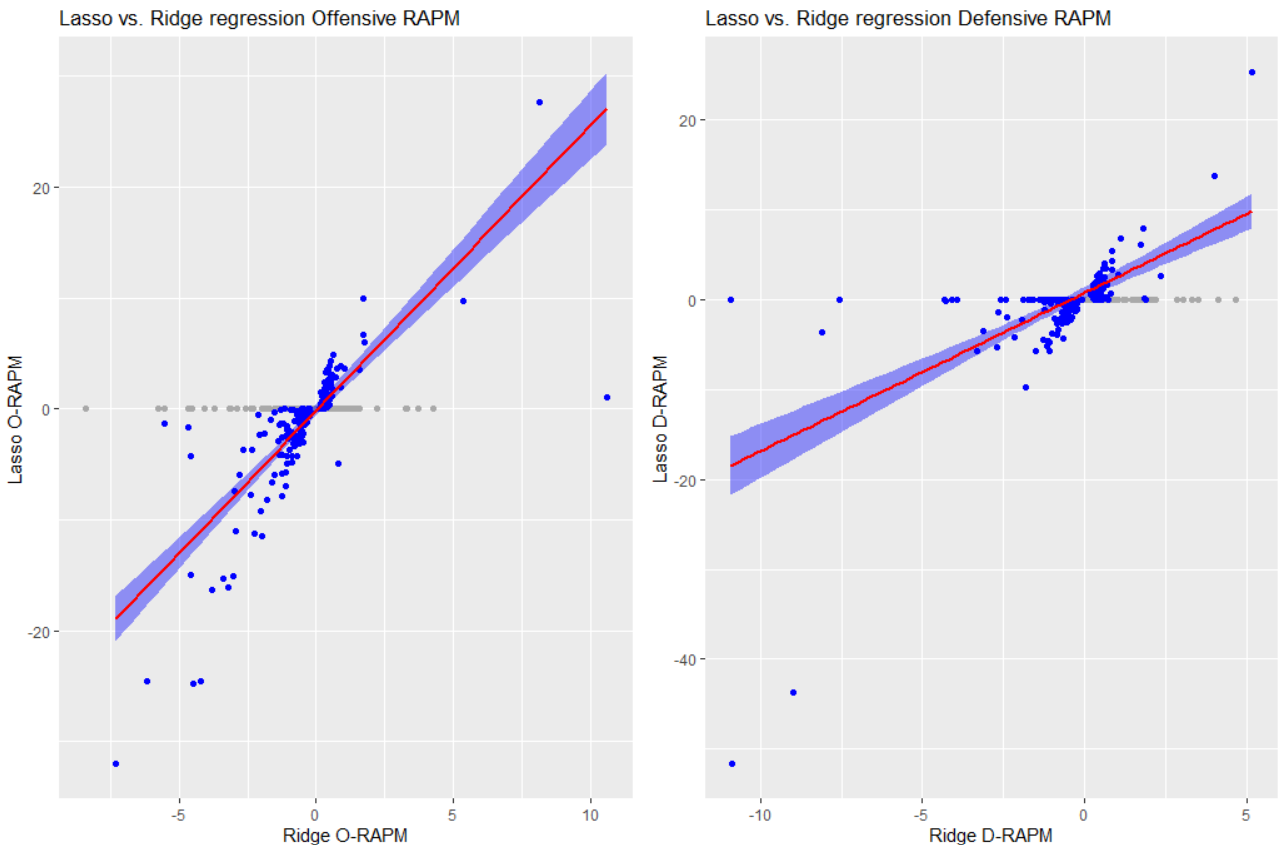
Figure 1: Ridge vs. lasso regression RAPM ratings (considering all players)

2.3.3 Filtering low-time players (LTPs)

Although lasso outperforms ridge, some LTPs still seem to have an impact on the evaluation metrics. A possible solution to improve the lasso ratings might be to exclude LTPs from our analysis as already suggested in the relevant bibliography. Therefore, we have implemented both regularization methods (lasso and ridge) after removing 232 players with less than 200 minutes played (filtered dataset). This threshold value is comparable with similar choices in the literature: [9] used data for players with more than 250 minutes played in two seasons 2002-2004, while [6] used a higher threshold of more than 300 minutes played in the 2007-2008 season.

Before removing LTPs from the dataset, we implemented an intermediate step where all players with a playing time of less than 200 minutes (LTPs) were considered as a reference group with the same RAPM. The ratings obtained from this intermediate step were found to be similar and highly correlated with those obtained after their removal. Therefore, we decided to proceed with the latter analysis, which is commonly adopted in the literature.

The filtered dataset now consists of 485 players (out of 717 in the original dataset) in which we obtain a total of 970 RAPMs in total (offensive and defensive ones). In this filtered dataset, estimated ridge and lasso RAPMs exhibit higher correlation ($78.8\%$ and $73.9\%$ for offensive and defensive RAPMs, respectively) than those obtained from the full dataset ($60\%$ and $55.2\%$, respectively). This correlation further increases to $90\%$ if we consider only the non-zero lasso RAPMs.

Although results improved in both approaches when using the filtered dataset, the ridge-based RAPMs did not show sufficient improvement, as they tend to prioritise unexpectedly performed players at the top of their rankings. For instance, only $28\%$ of the top 100 offensive and defensive ridge RAPMs consisted of starter players. This marks a substantial improvement compared to the corresponding percentage of $8\%$ when all players were included in the analysis. However, this improvement does not appear to be adequate.

On the other hand, lasso-based RAPMs showed a greater improvement. For instance, $42\%$ of the top-50 offensive and defensive RAPMs were starters in the full dataset, while for the filtered dataset this percentage increased to $55\%$. Furthermore, the distribution of the playing time for the top-50 players in the filtered dataset was left-skewed. This implies that the majority of the top-rated players had high playing time (Figure 2).

Despite the improved promising results of the lasso RAPMs in the filtered dataset, we will further explore the implementation and the development of RAPMs based on the multinomial logistic regression model which is more appropriate for the outcome variable of interest here i.e. the number of points scored per possession. In the following, we continue our analysis using the filtered dataset. Before we proceed to the more complex case of the multinomial logistic regression model, we will first implement the simpler binary logistic model, where the response variable is simply whether the team in possession scored or not. This is the first step towards the final goal of fitting the more advanced multinomial logistic regression model. As we will show later, this also allows us to provide an indirect approximate interpretation for the simple regression-based approach.

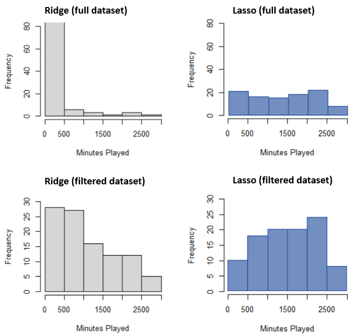
Figure 2: Minutes played of top 50 offensive and 50 defensive ridge (grey) and lasso (blue) RAPM players for the full (first row) and the filtered dataset (second row).

2.3.4 Logistic regression with shrinkage methods

In this section, we proceed by considering as a response variable $Y_{i}$ which records whether the team in possession scored or not. Since this simplified response is now binary, we will consider a standard, Bernoulli-based, logistic regression model given by

$$Y_{i} = {\cal I}(Pts_{i}>0),\mbox{~{}~{}with ~{}~{}}Y_{i}\sim Bernoulli(P_{i})\mbox{~{}~{} and ~{}~{}}P_{i}=\frac{1}{1+e^{-\mu_{i}}}$$ (2)

for $i=1,\dots,n$; where $\mu_{i}$ is the linear predictor as defined in the normal linear model formulation (1), ${\cal I}(A)$ is the indicator function taking the value of one if $A$ is true and zero otherwise and $P_{i}$ is the probability of scoring in $i$ possession.

The estimated coefficients $\beta_{k}^{o}$ and $\beta_{k}^{d}$of each $k$ player’s offensive and defensive dummy variables $X_{ik}^{o}$ and $X_{ik}^{d}$ are measures of their contribution to their team’s scoring ability (in the form of binary outcome). These coefficients can be considered as RAPMs on a different scale since they measure the effect of each player in terms of log-odds of scoring.

For the estimation of logistic regression RAPMs, we have similarly applied regularization methods as in the normal-based RAPMs. For both ridge and lasso methods, the RAPM-based ranking where obtained using the shrinkage parameter value $\lambda_{min}$ obtained from a 10-fold cross-validation. The lasso implementation resulted in 200 player RAPMs (either offensive or defensive) which were shrunk to zero. This represented approximately the $20\%$ of the total estimated RAPMs (and players, respectively).

From Binomial analysis, the correlation between RAPM ratings derived from the ridge Binomial ($\text{RAPM}^{\text{B}}$) and ridge Normal ($\text{RAPM}^{\text{N}}$) methodologies reveals an interesting result. Specifically, from our analysis, we found a significant linear relationship between these two RAPM ratings, as illustrated in Figure 3, expressed by the following equation:

$$\text{RAPM}^{\text{B}}_{k}=0.02\times\text{RAPM}^{\text{N}}_{k}+\varepsilon_{k},\quad\varepsilon_{k}\sim\mathcal{N}(0,0.008^{2})$$ (3)

for all $k=1,\ldots,K$ players (offender or defender), with $R^{2}\approx 0.89$. This equation allows us to compute the Binomial RAPMs from those derived under the Normal distribution. This capability enhances the interpretability of Normal RAPMs by providing additional insights. Moreover, it provides a reasonable theoretical justification for using the normal RAPMs as approximations of the binomial RAPMs, which are derived from a model which is properly defined with a correctly specified distribution.

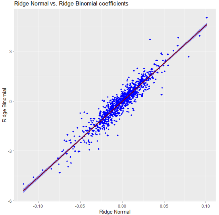
Figure 3: Coefficients of ridge Binomial vs ridge Normal model.

Although the logistic regression RAPMs can be considered an improvement when compared to the normal-based RAPMs, it does not consider the scoring information that is inherent in basketball, as they disregard the exact number of points scored. Therefore, this model should be further extended to account for the different number of points scored in each offence/possession. This is crucial, as each scoring category (one, two or three-pointers) demands different skills from the players and strategies from the team.

2.3.5 Multinomial logistic regression with shrinkage methods

In this section, we proceed with the implementation of a multinomial logistic regression for modelling the scoring outcome of each possession. As we have already discussed, this approach is more appropriate for our problem since it can model separately each of the types of scores. In this way it accounts for different scoring contributions of each player.

Due to the large size of the data, for computational efficiency, the multinomial model was fitted indirectly by using three binomial models for the three scoring categories under consideration (one, two and three or more points per possession versus no points).

Following the methodology implemented in normal models, for each of the three models, lasso regularization is used as a shrinkage method with the penalty parameter $\lambda$ set to the value which attains the minimum RMSE ($\lambda=\lambda_{min}$).

Hence, we consider the following model formulation

$$Y_{i}^{\mathcal{M}}=Pts_{i},\mbox{~{}for~{}}Pts_{i}\in\{0,1,2\}\mbox{~{}and~{}}Y_{i}^{\mathcal{M}}=3,\mbox{~{}for~{}}Pts_{i}\geq 3$$

with

$$Y_{i}^{\mathcal{M}}\sim Multinomial(\boldsymbol{\pi}_{i})\mbox{~{}and~{}}\boldsymbol{\pi}_{i}=(\pi_{i0},\pi_{i1},\pi_{i2},\pi_{i3})\mbox{~{}with~{}}\sum_{\ell=0}^{3}\pi_{i\ell}=1.$$ (4)

The Multinomial probabilities are given via the following equations

$$\pi_{i\ell}=\frac{e^{\mu_{i\ell}}}{1+e^{\mu_{i1}}+e^{\mu_{i2}}+e^{\mu_{i3}}}\mbox{~{}for~{}}\ell=0,1,2,3;$$ (5)

where $\pi_{i0},\pi_{i2},\pi_{i2},\pi_{i3}$ are the probabilities of no scoring, scoring one point, two points or three points (or more) in $i$ possession. The linear predictor $\mu_{i\ell}$ is given by

$$\mu_{i\ell}=b_{0\ell}+\sum_{j=1}^{p}b_{j\ell}X_{ij}+\sum_{k=1}^{K}\beta^{o}_{k\ell}X_{ik}^{o}+\sum_{k=1}^{K}\beta^{d}_{k\ell}X_{ik}^{d},\mbox{~{}for~{}}\ell=1,2,3\mbox{~{}and~{}}\mu_{ik}=0,$$ (6)

for $i=1,\dots,n$.

We implemented the multinomial regression formulation by considering three separate binomials given by

$$Y_{i}^{(\ell 0)}\!\!\! = \!\!\!\left\{\begin{array}[]{ll}{\cal I}(Pts_{i}=\ell)&\!\!\mbox{when~{}}Pts_{i}\in\{0,\ell\}\\ NA&\!\!\mbox{otherwise}\end{array}\right.,\mbox{~{}with~{}}Y_{i}\sim Bernoulli\big{(}P_{i}^{\ell 0}\big{)}\mbox{~{}and~{}}\log\frac{P_{i}^{\ell 0}}{P_{i}^{00}}=\mu_{i\ell}.~{}~{}~{}$$ (9)

From the above-fitted models, we obtain the multinomial probabilities using Eq. 5. Note that the estimates based on the separate logistic regression approach are less efficient with larger standard errors than the direct multinomial logistic approach. Nevertheless, the loss is minor when the baseline category is dominant on the data like in our case [1, Chap. 8]. We prefer the separate logistic regression approach here for two reasons. First, the separate regression approach offers advantages in terms of computational efficiency. Hence, it can be implemented for datasets with large sample sizes, as in the present study. Secondly, this approach allows us to implement different variable selection and shrinkage algorithms on the effects of each scoring category. By this way, we can identify the contribution of each player in the three different types of scores.

Team effects were not included in the fitted model, since they were not found to be significant. In the final multinomial model, 362 offensive and 316 defensive players actively contributed to the model. These were players with non-zero RAPMs in at least one of the binomial components. In this way, if a player has a significant impact in at least one scoring situation, his effect is taken into consideration in the final model formulation.

Although our approach is beneficial and more informative than the simple regression or logistic regression approach in the sense that we identify the contribution of each player at the different types of scores, in the end, we would like to summarize the offensive and the defensive contribution of each player with an overall index. For the offensive contribution of a player, this can be achieved by calculating the expected number of points (in a single possession) scored by the team of this player when he is included in the lineup and all other players on the court are from the reference category (with zero RAPM) – denoted by $EPTS^{o}_{k}$ . Similarly, the defensive contribution of a player can be evaluated by the expected number of points (per possession) conceded from the team of this player when he is not included in the lineup and all other players on the court are from the reference category (with zero RAPM). Equivalently, this is denoted by $EPTS^{d}_{k}$ Hence, the EPTS ratings are defined as

$$EPTS^{r}_{k}=E(Pts_{i}|X_{ik}^{r}\neq 0,{\bf X}^{r}_{i\setminus k}={\bf 0},{\bf X}^{\overline{r}}_{i}={\bf 0})\mbox{~{}for~{}}r\in\{o,d\}.$$

for $k=1,\ldots,485$. The two measures of the expected number of points, $EPTS^{r}_{o}$ and $EPTS^{r}_{d}$, will be functions on the offensive and defensive coefficients of the fitted multinomial regression model. Under this perspective, the expected number of points (EPTS) will be obtained by

$$EPTS^{r}_{k}=\Pi^{r}_{k1}+2\times\Pi^{r}_{k2}+3.01\times\Pi^{r}_{k3},~{}r\in\{o,d\};~{}~{}\overline{r}=\{o,d\}\setminus r$$ (10)

with $\Pi^{o}_{k\ell}$ for $\ell\in\{1,2,3\}$ being estimated by the multinomial logistic regression probabilities of scoring one, two or three points and more, respectively, per possession from the team of player $k$ when he is included in the lineup under a specific simplified scenario. This scenario is the case where all teammates of player $k$ in the lineup and opponents are players included in the reference group (i.e. with zero regression coefficients). Similarly, $\Pi^{d}_{k\ell}$ (for $\ell\in\{1,2,3\}$) are the probabilities of scoring one, two or three points and more, respectively, per possession by the opponent of the team of player $k$ when he is not included in the lineup under the same simplified scenario. Under this simplified scenario, the point probabilities are given by

$$\Pi^{r}_{k\ell}=\dfrac{e^{\mu^{r}_{k\ell}}}{1+e^{\mu^{r}_{k1}}+e^{\mu^{r}_{k2}}+e^{\mu^{r}_{k3}}}\mbox{~{}~{}with~{}~{}}\mu^{r}_{k\ell}=b_{0\ell}+b^{r}_{k\ell}\,,$$ (11)

for $\ell\in\{1,2,3\}$. The above overall evaluation score is now based on the RAPM coefficients of the specific type of points and additionally to the constant terms which adjust calculations over the simplified scenario where the rest of the players come from the reference group (with zero RAPM coefficients).

The Root Mean Squared Error (RMSE) of the fitted multinomial model is lower compared to the Normal model ($1.62<1.86$). To further assess the model’s fit, we simulated 1,000 samples from a multinomial distribution using the estimated probabilities per possession. The resulting relative frequencies of points per possession closely resemble those observed in the actual data (Figure 4) at the marginal level. A bootstrap chi-square test revealed no statistically significant difference between the marginal fitted frequencies and the observed ones (p-value = $0.55>0.05$). This finding suggests a good fit of the model.

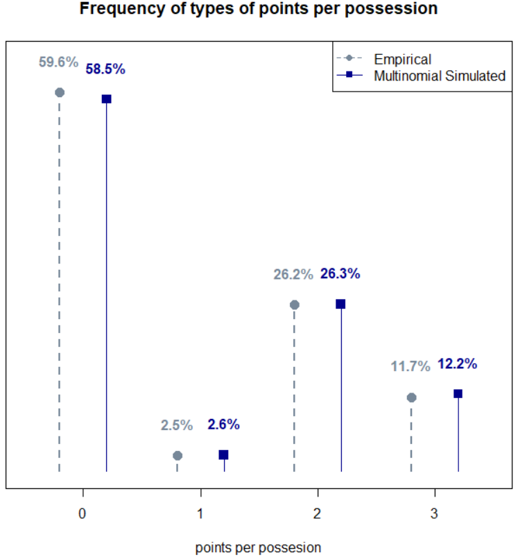
Figure 4: Relative frequencies of actual points per possession vs. the simulated by the lasso Multinomial model.

3 Results

This section presents the key findings obtained by applying the methodological procedures outlined earlier in this work. Our focus lies on comparing the RAPM approaches presented in previous sections. We demonstrate the superiority of the multinomial lasso-RAPMs (EPTS and WEPTS) compared to the ones obtained with ridge and lasso normal models. Prior to this comparison, we establish the external validation criteria that serve as the basis for evaluating the performance of the different approaches.

3.1 External Validation Criteria

To evaluate the ratings generated by the implemented models, we compare them by using a series of validation criteria that can be thought as external and “objective”, due to their non-involvement in the model formulation. While the offensive RAPMs yielded promising results, the performance of the defensive RAPMs offers room for improvement. This might be due to the nature of defensive play in basketball. Unlike offensive performance, which can be more readily influenced by individual player skill, defensive success is often based on effective team cooperation and collaboration.

To evaluate the performance of the different RAPM approaches, we select the following set of external validation criteria:

• All NBA Teams Criterion: This criterion examines the percentage of top RAPM players per position who are included in the “best 3 lineups” (15 players in total) which are announced according to the official NBA website (https://www.nba.com/). As top-ranked RAPM players, we consider the six best players for each position except for the centers, where only the top three RAPM-ranked players are included.

• Low Time Players Criterion: We identify the bottom 50 players in terms of playing time and measure the percentage of top-50 RAPM players within this group. This criterion assesses whether the RAPM approach effectively reduces the influence of players with minimal playing time.

• Starters Criterion: We consider the percentage of top-50 offensive and defensive RAPM-based metrics (total of 100 players) that are classified as “starters”. All top-six most played players per team are considered as starters.

• Top-50 Box Score Statistics Criterion: This criterion identifies the top-50 players based on a variety of box score statistics (points, assists, and offensive rebounds for offence; defensive rebounds, steals, and blocks for defense). We then measure the percentage of these players who are included in the top-50 RAPM rankings.

3.2 Ridge vs. Lasso RAPM Normal Metrics

As a first step in our analysis, we compare the lasso RAPMs with more traditional ridge-based RAPMs commonly implemented in basketball analytics literature. The findings are quite promising in favour of the lasso approach. Specifically, the lasso method appears to outperform ridge regression based on the evaluation criteria established in Section 3.1.

An examination of Tables 1 and 2 reveals the superiority of lasso over ridge. Specifically, focusing on the playing time of top-rated players (Criterion 2), as shown in Table 1, our analysis highlights a clear advantage of lasso RAPMs over ridge. We observe that 14% of the top 100 players in the ridge RAPM rankings are among those with the lowest recorded playing time. This percentage drops to 3% for lasso Normal and 6% for the OLS ratings after removing the zero-contributed players indicated by lasso. The latter will be referred to as after-lasso RAPMs. This suggests a more accurate performance of the lasso models since it is generally unexpected for players with minimal in-season playtime to appear in the list with the highest contributions. This is a common behaviour of the plus/minus ratings found in ridge RAPMs, but restricted in the lasso approach.

On the other hand, a strong presence of starters among top performers is highly desirable. Examining the third criterion (Criterion 3a in Table 1), we observe that 55% and 50% of the players with the highest contributions are starters according to the lasso and after-lasso RAPMs, respectively. These percentages are about double (increased by 96% and 79%, respectively) the corresponding percentage (28%) achieved when using the ridge RAPMs.

While a high proportion of starters among top performers is desirable, the presence of starters among low performers requires further examination (Criterion 3b in Table 1). Interestingly, the lasso RAPM ratings include a higher percentage of starters (23% and 19% for lasso and after-lasso, respectively) compared to ridge RAPM (7%). However, this observation does not necessarily favour the ridge approach. A possible explanation is that, on some occasions, a player might be included in the starting roster due to a lack of better alternatives or his role in the team might be offensive and not defensive (or vice-versa).

Table 1: Comparison of validation Criteria 1–3 between RAPM ratings for the Normal models.

Model	Criterion #1	Criterion #2	Criterion #3a	Criterion #3b
Ridge Normal	27%	14%	28%	7%
Lasso Normal	40%	3%	55%	23%
Normal (after-lasso)	33%	6%	50%	19%
Criterion #1: All-NBA teams, Criterion #2: Low-time players in 100 top-RAPM, Criterion #3a: Starters in 100 top-RAPM and Criterion #3b: Starters in 100 bottom-RAPM; Bold indicates the maximum value by column/criterion

An examination of the box-score statistics of the top-rated RAMP players (Criterion 4 in Table 2) further strengthens the case in favor of lasso RAPMs. From this table, we observe a clear advantage for lasso RAPMs, particularly when compared to the performance of ridge based top players in key metrics such as points scored, assists, defensive rebounds, and blocks.

Table 2: Comparison of External Validation Criterion 4 for Lasso Normal ratings.

Model	PTS	AST	OREB	DREB	STL	BLK
Ridge Normal	30%	20%	12%	10%	18%	4%
Lasso Normal	42%	26%	14%	8%	14%	12%
Normal (after-lasso)	44%	30%	12%	20%	22%	12%
PTS: points scored per game, AST: assists per game, OREB: offensive rebounds per game, DREB: defensive rebounds per game, BLK: blocks per game, STL: steals per game; Bold indicates the maximum value by column/box-score

Further visual inspection of the distribution of the playing time (see Figure 5) suggests that the ridge model assigns high rankings to players with lower playing time, despite their lower scoring outputs (see Figure 6). This is also supported by the finding that at least 75% of the top 50 ridge RAPM players score no more than 15 points per game (Figure 6). In contrast, lasso models prioritize players with both higher playing time and higher scoring performances. This is evident by the fact at least 75% of the top performers in the offensive lasso (and after-lasso) RAPMs score around 20 and 18 points per game, respectively.

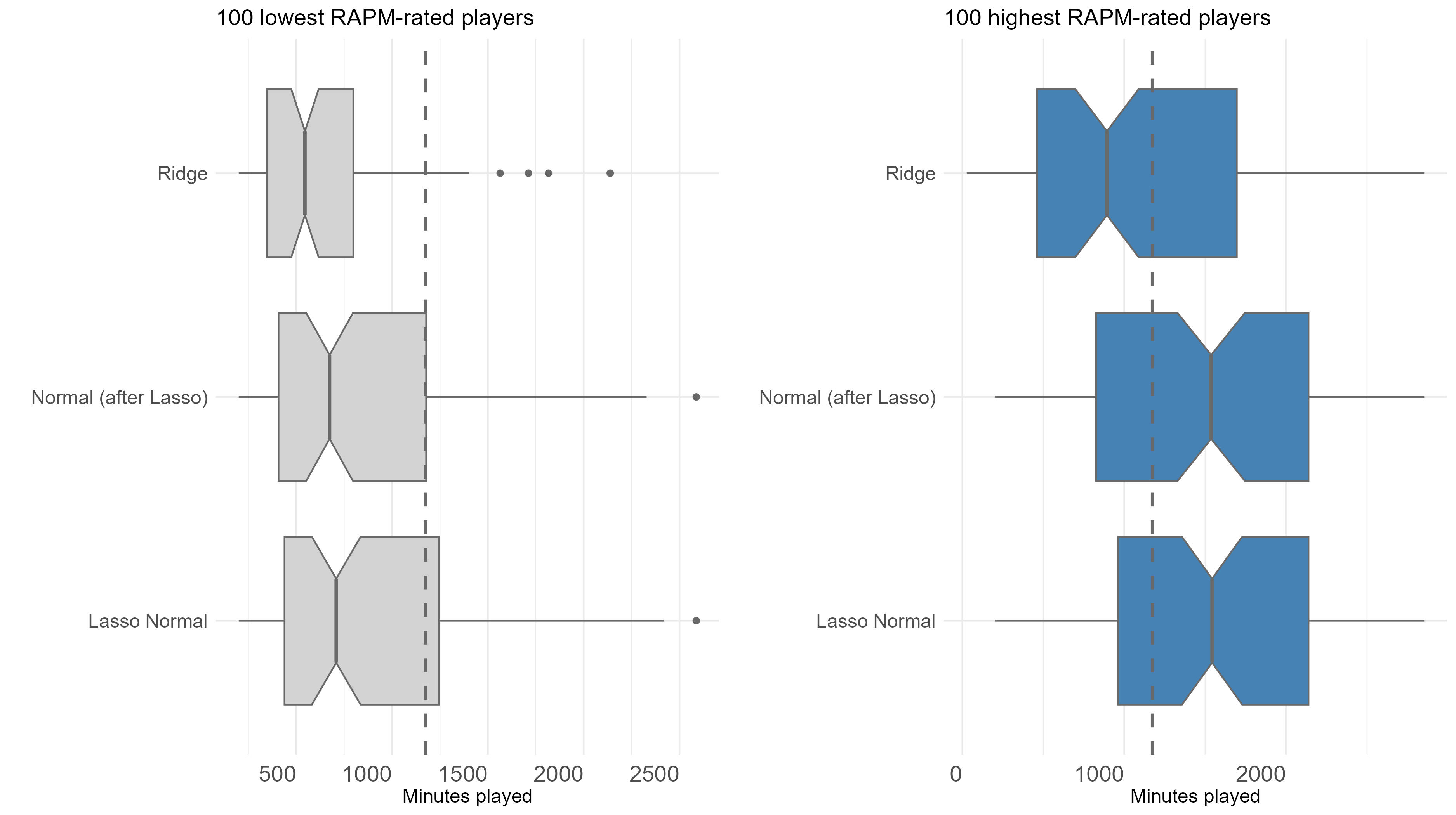
Vertical dashed line is a threshold of the lowest playing time observed in starters.

Figure 5: Minutes Played of players in top and bottom 100 (50 offensive and 50 defensive) RAPMs.

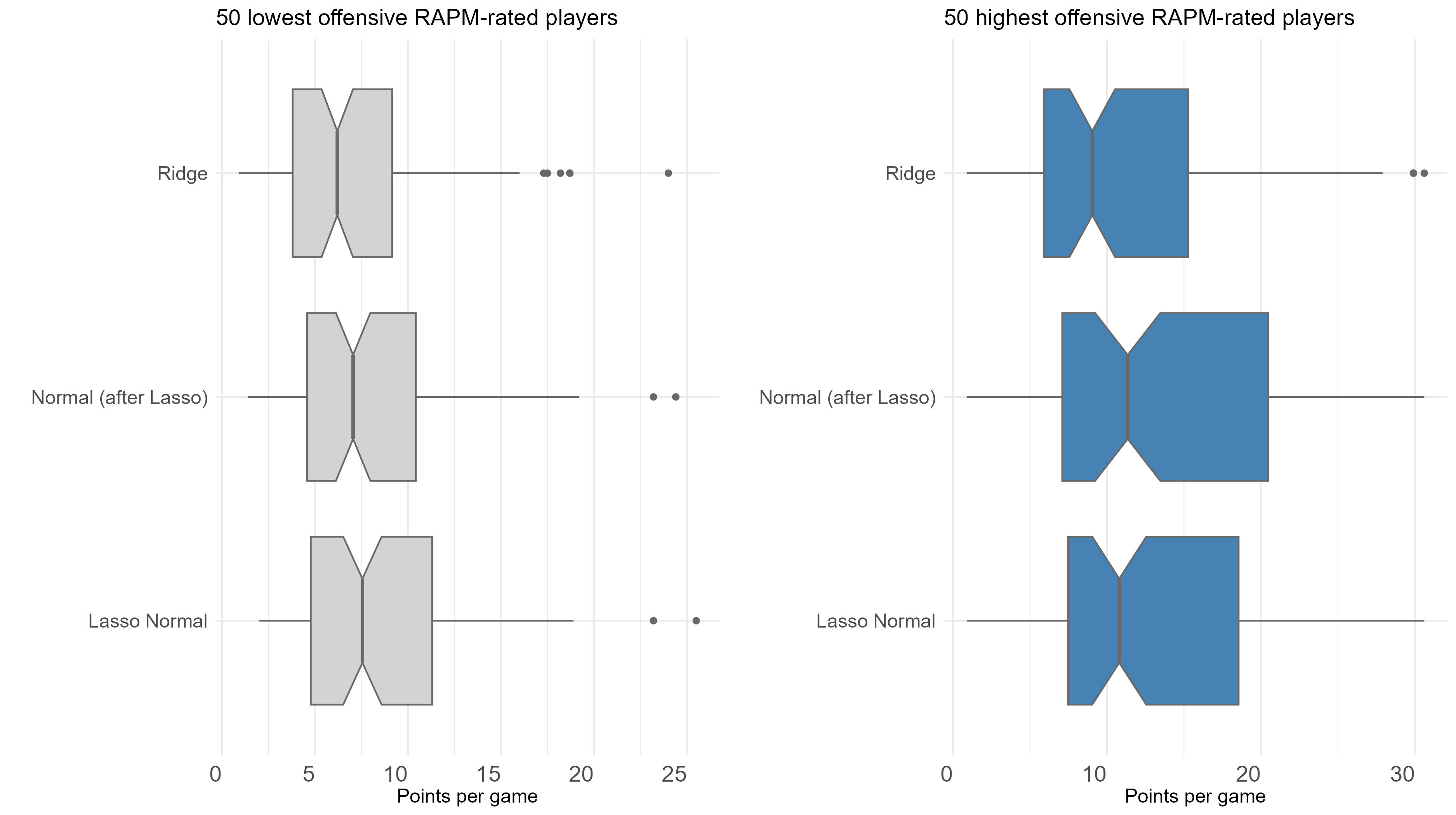
Figure 6: Points scored per game by players in top and bottom 100 (50 offensive and 50 defensive) RAPMs.

To conclude with, based on the external validation criteria, our findings suggest that the lasso methodology offers ratings that lead to better player discrimination. Moreover, it yields more reasonable ratings compared to ridge regression. One potential drawback of ridge regression appears to be its handling of players with limited playing time. Ridge regression may overestimate or underestimate the performance of low-time players, potentially assigning them to extreme ranking positions (highest or lowest). Based on the validation criteria, a comparison between the lasso RAPMs and the after-lasso ratings revealed no substantial differences. Nevertheless, in the following, we favour the use of the ratings obtained from the lasso approach. This preference is because the latter ratings are directly obtained while the free-of-bias (due to the penalty of the lasso method) estimates, after-lasso RAPMs, need extra computational effort after the initial screening procedure using lasso.

3.3 Lasso Normal vs. Multinomial

After demonstrating the superiority of the lasso technique over ridge regression in Section 3.2, we proceed here to examine the normal and multinomial RAPMs inside the lasso framework. As discussed in Section 2.3.5, the proposed multinomial model accounts for the discrete nature of points scored per possession. This choice, in combination with lasso and its shrinkage properties, offers a clear advantage over the commonly used ridge regression RAPMs. Therefore, in this section, we will examine and compare the external validation criteria (see Section 3.1) for both the lasso multinomial and Normal models.

From Tables  3 and 4 we observe small differences in the performance, with no clear winner between the two distributions for the different evaluation criteria. The lasso multinomial performs better in two out of four evaluation criteria presented in Table 3. When analyzing players from “All NBA teams” (Criterion 1), lasso multinomial outperforms the corresponding normal model by identifying a larger proportion of such players ($47\%$ vs. $40\%$). Furthermore, in Criterion 3b, the multinomial lasso performs marginally better than the standard lasso since fewer starters are included in the bottom 100 list ($20\%$ vs $23\%$). On the other hand, Normal-based RAPMs outperform the multinomial ones in Criterion 2, since a lower proportion of low-time players ($3\%$ vs. $9\%$) is included in its top 100 player rankings. Finally, regarding Criterion 3a, a higher proportion of starters are included in the top-100 RAPM list ($55\%$ vs. $47\%$). Regarding the box-score statistics (Criterion 4) of top-rated players, lasso multinomial is marginally better than normal lasso in all statistics except the number of points (PTS); see Table 4.

Table 3: Comparison of validation Criteria 1–3 between ratings for the lasso Normal and Multinomial models.

Model	Criterion #1	Criterion #2	Criterion #3a	Criterion #3b
Lasso Normal	40%	3%	55%	23%
Lasso Multinomial	47%	9%	47%	20%
Criterion #1: All-NBA teams, Criterion #2: Low-time players in 100 top-RAPM, Criterion #3a: Starters in 100 top-RAPM and Criterion #3b: Starters in 100 bottom-RAPM; Bold indicates the maximum value by column/Criterion

Table 4: Comparison of External Validation Criterion 4 for Lasso Ratings of Normal and Multinomial.

Model	PTS	AST	OREB	DREB	STL	BLK
Lasso Normal	42%	26%	14%	8%	14%	12%
Lasso Multinomial	38%	28%	16%	14%	20%	14%
PTS: points scored per game, AST: assists per game, OREB: offensive rebounds per game, DREB: defensive rebounds per game, BLK: blocks per game, STL: steals per game; Bold indicates the maximum value by column/box-score

From the previous comparisons, we conclude that the lasso multinomial performs somewhat better than the standard approach. Furthermore, the multinomial model is more realistic than the standard normal approach since the response is properly considered as a discrete random variable, whereas the latter approach (incorrectly) assumes that the number of points per possession is a continuous random variable. Finally, the choice of the multinomial model is further supported by the fact that the RAPMs in conventional lasso models are shrunk to zero for around $70\%$ of the players. In contrast, the corresponding proportion for the lasso multinomial model is reduced to only $30\%$. Since the goal is to develop an evaluation metric, reducing the RAPM for the majority of players to zero implies that, for a large number of players, no clear evaluation and discrimination from the “average” level will be provided.

4 A New Improved Evaluation Metric: Weighted Expected Points (wEPTS)

4.1 The metric

In this section, we proceed by introducing an improved weighted version of EPTS which takes into consideration the participation of each player throughout the season. The goal of this evaluation metric is to quantify the expected points per possession for the team of the player under study. We will evaluate two different lineup configurations: one lineup including the player of interest and a second one without the player of interest. All other players on the court are assumed to belong to the reference category. The corresponding expected points of these two line-ups will be weighted according to weighted according to the proportion of possessions in which the player of interest participated.

Hence, the weighted Expected Points (wEPTS) per possession is defined as the expected team points per possession for the team of $k$ player when all other players are from the reference group with the zero-lasso RAPMs and it is given by

$$wEPTS^{r}_{k} = E(Pts_{i}|{\bf X}^{r}_{i\setminus k}={\bf 0},{\bf X}^{\overline{r}}_{i}={\bf 0},T_{i}=t_{k})$$ (12)

$$= ~{}~{}~{}~{}P(X_{ik}^{r}\neq 0|T_{i}=t_{k})E(Pts_{i}|X_{ik}^{r}\neq 0,{\bf X}^{r}_{i\setminus k}={\bf 0},{\bf X}^{\overline{r}}_{i}={\bf 0})$$

$$+P(X_{ik}^{r}=0|T_{i}=t_{k})E(Pts_{i}|X_{ik}^{r}=0,{\bf X}^{r}_{i\setminus k}={\bf 0},{\bf X}^{\overline{r}}_{i}={\bf 0})$$

$$= W_{k}^{r}\,EPTS_{k}^{r}+(1-W_{k}^{r})\,EPTS_{0}^{r}$$

where $r\in\{o,d\};~{}~{}\overline{r}=\{o,d\}\setminus r$ . Moreover, the weight $W^{r}_{k}$ is estimated by

$$\widehat{W}^{r}_{k}=\frac{n^{r}_{k}}{n^{r}_{t_{k}}}=\dfrac{\sum_{i=1}^{n}{\cal I}(X_{ik}^{r}\neq 0)}{\sum_{i=1}^{n}{\cal I}(T_{i}^{r}=t_{k})},$$

and ${\cal I}(A)$ is the indicator function taking value one if $A$ is true and zero otherwise; $T_{i}$ is the team in offence/defence in possession $i$, $t_{k}$ is the team of player $k$, $X^{r}_{ik}$ is the binary dummy variable for player $k$ taking zero-one values in offensive ratings and minus one-zero in the defensive ratings, $({\bf X}^{r}_{i\setminus k}={\bf 0},{\bf X}^{\overline{r}}_{i}={\bf 0})$ implies that all other players except for the player of interest are set equal to players belonging to the reference group, $n^{r}_{t_{k}}$ is the number of possessions that the team of player $k$ is in offence or defence (depending on $r$), $n^{r}_{k}$is the number of possessions that the player $k$ is included in the playing lineup of the team in offence or defence. Finally, $EPTS_{k}^{r}$ are the expected points of player $k$ as defined (10) while $EPTS_{0}^{r}$ are the expected points of the reference lineup, given by

$$EPTS_{0}^{r}=\dfrac{e^{b_{01}}+2e^{b_{02}}+3.01e^{b_{03}}}{1+e^{b_{01}}+e^{b_{02}}+e^{b_{03}}}\mbox{ for}~{}r\in\{o,d\}.$$ (13)

The wEPTS rating has a similar interpretation to EPTS. The primary distinction is that we now consider the conditional expectation of the points for a reference lineup with and without the player of interest weighted by the proportion of possessions in which the player of interest participates on his team. Overall, this index acts as a shrinkage method on EPTS shrinking them towards the expected points of the reference group for players with minimal playing time. On the other hand, if we consider the case of a player who participates in all possessions of his team (which is not a realistic case in practice) then the $wEPTS$ will become equal to the $EPTS$. Finally, the new index only requires minimal extra computations since we only need the proportion of possessions that each player participates in his team and to calculate the expected points of the reference group $EPTS_{0}^{r}$ given by (13) which is nevertheless, directly available from the lasso coefficients.

4.2 Weighted EPTS (wEPTS) through validation criteria

We proceed with the comparison of wEPTS with the EPTS rankings and the RAPMs from the lasso-normal approach with respect to the external validation criteria we have introduced in Section 3.1.

Tables 5 and  6 demonstrate the superiority of the weighted EPTS across various criteria. Furthermore, when examining the list of players with the highest EPTS and wEPTS ratings, we reveal that the average playing time per game is 26.3 and 29.7 minutes, respectively. Furthermore, among these top-rated players, the average points scored per game are 15.1 and 17.8 for EPTS and wEPTS, respectively. Concurrently, when considering players with the lowest offensive EPTS ratings, they demonstrate considerably higher points, on average, than the corresponding bottom list players of offensive wEPTS, averaging 16.6 and 9.6 points per game, respectively.

Table 5: Comparison of External Validation Metrics for Criteria 1–3 for Lasso Ratings (Normal, Multinomial and weighted Multinomial).

Rating (Model)	Criterion #1	Criterion #2	Criterion #3a	Criterion #3b
RAPM (Normal)	40%	3%	55%	23%
EPTS (Multinomial)	47%	9%	47%	20%
wEPTS (Multinomial)	67%	2%	74%	45%
Criterion #1: All-NBA teams, Criterion #2: Low-time players in 100 top-RAPM, Criterion #3a: Starters in 100 top-RAPM and Criterion #3b: Starters in 100 bottom-RAPM; Bold indicates the maximum value by column/Criterion

Table 6: Comparison of External Validation Criterion 4 for Lasso Ratings (Normal, Multinomial and weighted Multinomial).

Model	PTS	AST	OREB	DREB	STL	BLK
RAPM (Normal)	42%	26%	14%	8%	14%	12%
EPTS (Multinomial)	38%	28%	16%	14%	20%	14%
wEPTS (Multinomial)	44%	36%	14%	22%	28%	22%
PTS: points scored per game, AST: assists per game, OREB: offensive rebounds per game, DREB: defensive rebounds per game, BLK: blocks per game, STL: steals per game; Bold indicates the maximum value by column/box-score

Although wEPTS demonstrates clear superiority across (nearly) all selected validation criteria, a surprising result is found concerning Criterion 3b in Table 5. It becomes apparent that a higher proportion of starters appear in the list of players with the lowest wEPTS rankings compared to the corresponding list compiled by using EPTS ($45\%$ and $20\%$ respectively). However, none of the starters was found to be in the bottom list of both offensive and defensive ratings. This suggests that such starters are ranked in the bottom 50 list of offensive ratings due to their primary defensive role within the team, wherein their defensive contribution is considerably higher than their offensive performance. Conversely, all starters who appeared in the bottom 50 list of defensive ratings exhibit substantially higher offensive contributions, potentially indicative of their offensive responsibilities within the team.

4.3 Lasso vs. After-Lasso Ratings

The RAPM and EPTS ratings presented on the previous sections are based on biased “shrunk” estimates of model coefficients which quantify the contribution of each player. This section explores the impact of bias on RAPM and EPTS ratings. We compare two approaches: (a) using directly biased coefficients derived using lasso and (b) using the unbiased (MLE) coefficients, after removing players whose coefficients were flagged as zero by lasso. For the latter case we will use the conventional name “after-lasso” ratings.

Tables 7 and 8 present the performance of the two approaches (lasso and after-lasso) for the selected validation criteria. From these tables, there is no clear winner between the two approaches and there are minor differences in performance between the lasso coefficients and the after-lasso coefficients, particularly for the proposed wEPTS ratings. Given that the two approaches are similar in performance and the additional computational burden required to refit the model for after-lasso ratings, we recommend directly using the lasso coefficients for the calculation of wEPTS.

Table 7: Comparison of validation Criteria 1–3 between lasso and after-lasso ratings for the Normal RAPM, the Multinomial EPTS and the Multinomial wEPTS.

Model
(Rating)	Method	Criterion #1	Criterion #2	Criterion #3a
Normal	Lasso	40%	3%	55%
(RAPM)	After-lasso	33%	6%	50%
Multinomial	Lasso	47%	9%	47%
(EPTS)	After-lasso	33%	10%	40%
Multinomial	Lasso	67%	2%	74%
(wEPTS)	After-lasso	60%	2%	73%
Criterion #1: All-NBA teams, Criterion #2: Low-time players in 100 top-RAPM, and Criterion #3a: Starters in 100 top-RAPM

Table 8: Comparison of validation Criterion 4 between lasso and after-lasso ratings for the Normal RAPM, the Multinomial EPTS and the Multinomial wEPTS.

Model
(Rating)	Method	PTS	AST	OREB	DREB	STL	BLK
Normal	Lasso	42%	26%	14%	8%	14%	12%
(RAPM)	After-lasso	44%	30%	12%	20%	22%	12%
Multinomial	Lasso	38%	28%	16%	14%	20%	14%
(EPTS)	After-lasso	36%	30%	12%	14%	22%	14%
Multinomial	Lasso	44%	36%	14%	22%	28%	22%
(wEPTS)	After-lasso	50%	38%	16%	22%	34%	20%
PTS: points scored per game, AST: assists per game, OREB: offensive rebounds per game, DREB: defensive rebounds per game, BLK: blocks per game, STL: steals per game; Bold indicates the maximum value by method

5 Highlights and Discussion

Following the literature, we initially implemented ridge regression on the full possession dataset for the 2021-2022 NBA season. However, this approach was susceptible to the influence of low-time players (LTPs), whose limited playing time inflated their estimated contributions. To address this issue, we have investigated two different approaches: First, we have implemented lasso instead of ridge and, second, we have removed low-time players from RAPM estimation.

For the first approach, lasso regression promotes sparsity by setting specific coefficients equal to zero. This will be effective for less influential variables (players). This characteristic of lasso resulted in RAPM estimates with a clearer distinction between well-performed, average and low-performed players. Concerning LTPs, the problem was mitigated (but not diminished) by shrinking the coefficients of such players of them to zero (i.e. to the group of “average” players). On the other hand, the exclusion of LTPs (defined as less than 200 minutes for the season) also improved the performance of the RAPM ratings. For this reason, we have proceeded by combining the two strategies (i.e. implementing lasso without LTPs).

The lasso model demonstrated better performance when evaluated using external validation criteria (Section 3.1). However, a key characteristic of lasso, while advantageous in some respects, is its tendency to set coefficients to zero, effectively omitting players with doubtful contributions. However, in the normal model, lasso regression resulted in the shrinkage of approximately $70\%$ of the player coefficients to zero. Consequently, only the remaining $30\%$ of players have been assigned with non-zero RAPM ratings.

Given the discrete nature of the response variable, a logistic regression model is the logical next step in our analysis. Initially, a binary classification model was fitted, predicting the outcome of scoring versus not scoring. Regularized logistic regression was implemented, achieving an accuracy of approximately $55\%$. However, this approach provides a simplified solution to our problem, neglecting the actual number of points scored on each possession.

Despite the moderate accuracy, an intriguing finding emerged from the relationship between the ridge Binomial logistic and ridge Normal RAPMs. We observed a strong linear relationship between the ratings generated by these two models. This finding provides a compelling justification for using the Normal RAPMs, despite their initial limitation of being derived from a model which is not ideally suited for the use of the number of points as a response. The fitted linear relationship allows us to convert Normal RAPMs into logistic regression RAPMs, which are obtained through a methodologically sound approach. This conversion essentially transforms the Normal RAPM scores into a framework more appropriate for the binary outcome (scoring vs. not scoring), enhancing the interpretability of standard RAPM player performance metrics.

Finally, the multinomial model — which is more appropriate for this type of response — was applied to the number of points per possession. To circumvent computational issues and to introduce greater flexibility in terms of which lasso coefficients were set to zero, we employed three distinct binomial implementations. Moreover, the multinomial model has the benefit of providing more specific information about each player’s contribution to the various scoring formats (one, two, or three points). Higher-ranked players in terms of three-point shooting might be chosen to play, for instance, if a team requires a three-point shot at a critical moment of the game. It is not about players with great shooting percentages; rather, it’s about players who boost their team’s chances of scoring a particular type of points. Such players have a specific role in the team, as for example a center with ball-passing ability or a player who drives to the paint with ease and passes the ball to the desired player for a shot.

Finally, considering insights from the multinomial model, we introduce a novel RAPM metric: the Expected Points (EPTS). This metric is derived from a correctly specified model for the number of points scored. To further refine the analysis, we propose a weighted version of EPTS, denoted as wEPTS. This extension incorporates player participation within each team’s possessions, effectively handling the issue of inflated contributions observed with low-time players. In summary, EPTS is based on a statistically sound foundation for evaluating player performance based on expected points scored. Moreover, our evaluation using established validation criteria demonstrates that wEPTS outperforms all other approaches considered in this study.

To conclude, in this study, we have considered a variety of issues concerning the estimation of RAPM player ratings from possession-based NBA data. The main contributions of this paper are: (a) we introduce the use of lasso instead of ridge and demonstrate its superiority in terms of evaluations; (b) we offer a clear interpretation of commonly used normal ridge RAPMs through logistic regression coefficients; and finally, (c) we introduce novel RAPM metrics: Expected Points Scored (EPTS) and its weighted version (wEPTS) based on a multinomial logistic regression model, which is the statistically appropriate approach for modelling the points scored per possession. The proposed wEPTS has four clear advantages: First, it outperforms all other approaches evaluated in this study, including the standard ridge normal RAPMs. Secondly, it effectively addresses the challenge of low-time players, almost eliminating their inflated contributions. Third, it is based on a foundationally appropriate statistical model and, four, it can separately evaluate and consider the contribution of each player based on the different type of scoring points that each player contributes.

References

- \bibcommenthead
- Agresti [2013] Agresti A (2013) Categorical Data Analysis, 3rd edn. Wiley Series in Probability and Statistics, Wiley-Interscience
- Ghimire et al [2020] Ghimire S, Ehrlich JA, Sanders SD (2020) Measuring individual worker output in a complementary team setting: Does regularized adjusted plus minus isolate individual nba player contributions? PLOS ONE 15(8):1–11. 10.1371/journal.pone.0237920, URL https://doi.org/10.1371/journal.pone.0237920
- Hoerl [2020] Hoerl R (2020) Ridge regression: A historical context. Technometrics 62:420–425. 10.1080/00401706.2020.1742207
- Hvattum [2019] Hvattum LM (2019) A comprehensive review of plus-minus ratings for evaluating individual players in team sports. International Journal of Computer Science in Sport 18:1 – 23. URL https://api.semanticscholar.org/CorpusID:201734379
- Ilardi and Barzilai [2007] Ilardi S, Barzilai A (2007) Adjusted plus-minus: An idea whose time has come. URL http://www.82games.com/ilardi2.htm
- Ilardi and Barzilai [2008] Ilardi S, Barzilai A (2008) Adjusted plus-minus ratings:new and improved for 2007-2008. URL http://www.82games.com/ilardi2.htm
- Oliver [2002] Oliver D (2002) Basketball on Paper: Rules and Tools for Performance Analysis. Brassey’s, Inc, Washington D.C.
- Pelechrinis [2019] Pelechrinis K (2019) Calculating rapm. https://github.com/kpelechrinis/NBA_Tutorials/tree/master/rapm
- Rosenbaum [2004] Rosenbaum D (2004) Measuring how nba players help their teams win. URL http://www.82games.com/comm30.htm
- Sill [2010] Sill J (2010) Improved nba adjusted +/- using regularization and out-of-sample testing. Paper presented at the MIT Sloan Sports Analytics Conference, 6 March 2010
- Winston [2012] Winston W (2012) Mathletics. How gamblers, managers, and sports enthusiasts use mathematics in baseball, basketball, and football. Princeton University Press, New Jersey