TabularFM: An Open Framework For Tabular Foundational Models

Abstract

Foundational models (FMs), pretrained on extensive datasets using self-supervised techniques, are capable of learning generalized patterns from large amounts of data. This reduces the need for extensive labeled datasets for each new task, saving both time and resources by leveraging the broad knowledge base established during pretraining. Most research on FMs has primarily focused on unstructured data, such as text and images, or semi-structured data, like time-series. However, there has been limited attention to structured data, such as tabular data, which, despite its prevalence, remains under-studied due to a lack of clean datasets and insufficient research on the transferability of FMs for various tabular data tasks. In response to this gap, we introduce a framework called TabularFM, which incorporates state-of-the-art methods for developing FMs specifically for tabular data. This includes variations of neural architectures such as GANs, VAEs, and Transformers. We have curated a million of tabular datasets and released cleaned versions to facilitate the development of tabular FMs. We pretrained FMs on this curated data, benchmarked various learning methods on these datasets, and released the pretrained models along with leaderboards for future comparative studies. Our fully open-sourced system provides a comprehensive analysis of the transferability of tabular FMs. By releasing these datasets, pretrained models, and leaderboards, we aim to enhance the validity and usability of tabular FMs in the near future.

1 Introduction

Foundational models (FMs) undergo training on extensive datasets through self-supervised learning methods. These models learns crucial patterns and structures within the data autonomously, without human guidance. Following this, they are fine-tuned on downstream tasks utilizing smaller datasets with labeled data. Research has shown that if foundational models are pre-trained on large datasets resembling the downstream datasets, the learned patterns from pre-training can be leveraged for the downstream tasks, resulting in a substantial performance boost for the subsequent models He et al. (2016); Waswani et al. (2017); Lin et al. (2023).

Foundational models have been proposed to handle unstructured data across various domains, including vision He et al. (2016), text Waswani et al. (2017), and biomedical data like proteins Lin et al. (2023) or small molecules Ross et al. (2022). However, when it comes to structured data such as tables, the task of constructing foundational models remains largely unexplored. Several challenges arise in building foundational models for tabular data. First, the transferability of learning methods across tabular datasets remains an open question. Unlike texts or images, where neural architectures like CNNs LeCun et al. (2015) or Transformers Waswani et al. (2017) were introduced to learn transferable patterns, tabular data presents distinct challenges. These include variations in categorical value encoding and numerical value scales, resulting in higher noise levels. Second, despite the existence of public tabular datasets, they tend to be small and noisy. For instance, some contain a mixture of text data or temporal information, which diverges from structured data. Moreover, the sizes of these available datasets are considerably smaller compared to the texts used in creating large language models. As this is an emerging area of research, there is a lack of standard benchmarks and leaderboards for evaluating tabular foundational models. In a recent position paper (van Breugel and van der Schaar, 2024), the authors noticed that tabular foundation models remain largely unexplored compared to the abundance of text and image foundation models. For instance, the number of accepted papers on tabular foundation models at recent major machine learning conferences is less than three percent of those focused on text foundation models. In this work, we present TabularFM, a comprehensive framework for creating and benchmarking tabular foundational models. Our contributions can be summarised as follows:

• Datasets for training and benchmark tabular FMs: clean datasets comprising a total of 2,693 tables, meticulously curated from 1 million GitTables Hulsebos et al. (2023) and 43,514 tables crawled from Kaggle. We released pretrained FM models on the curated datasets, benchmark datasets, and associated leaderboards for evaluating tabular FMs.

• Additionally, we provide an open-source framework for creating and benchmarking tabular FMs. This framework encompasses state-of-the-art self-supervised generative learning methods, data transformation techniques, and evaluation tools.

• An analysis of the transferability of tabular foundation models highlights several key findings. In Subsection 4.1, we show that pretrained models using CTGAN and TVAE transfer effectively across various data splits, outperforming models trained from scratch. However, adding extra column metadata does not improve transferability. Transformers pretrained on textual data perform well on benchmarks, but finetuning them on tabular data often reduces performance, raising questions about the need for larger tabular datasets. Our analysis in Figure 3 indicates that certain general knowledge, like the correlation between hospital beds and urban population or the link between weight loss and polydipsia via polyuria, transfers well through pretraining.

2 Data Creation

In this section, we briefly discuss the process of data creation, which includes data acquisition and data cleaning. Since building foundational models requires clean data, this step is crucial to ensure that only high-quality data is retained for training.

2.1 Kaggle Dataset

Kaggle is a leading platform for data science, offering diverse datasets across fields like healthcare and finance. A key challenge in using Kaggle data is its varied formats, duplicated information, and noisy data, including numerical, categorical, and unstructured data like text or time series. Our initial step filters Kaggle datasets by file type and quality, prioritizing those with a usability rating of 8/10 or higher. This process identified 43,514 potential datasets. Further cleaning based on data type, missing values, and unique categorical values narrowed it down to 1,435 high-quality tables containing only numerical and categorical data. We developed two variations of the Kaggle dataset. The first uses a random split to create training, validation, and test subsets. The second uses domain-based splits, clustering table names BERT embeddings into 100 groups with $k$-mean and then randomly assigning these clusters to the subsets. Figure 1 shows a TSNE representation of the top 10 domains clustered by $k$-mean, illustrating clear separation in the projected space. This domain-based split aims to validate model transferability across domains. Detailed statistics are in Table 1, with further details on the cleaning and splitting process in the Appendix.

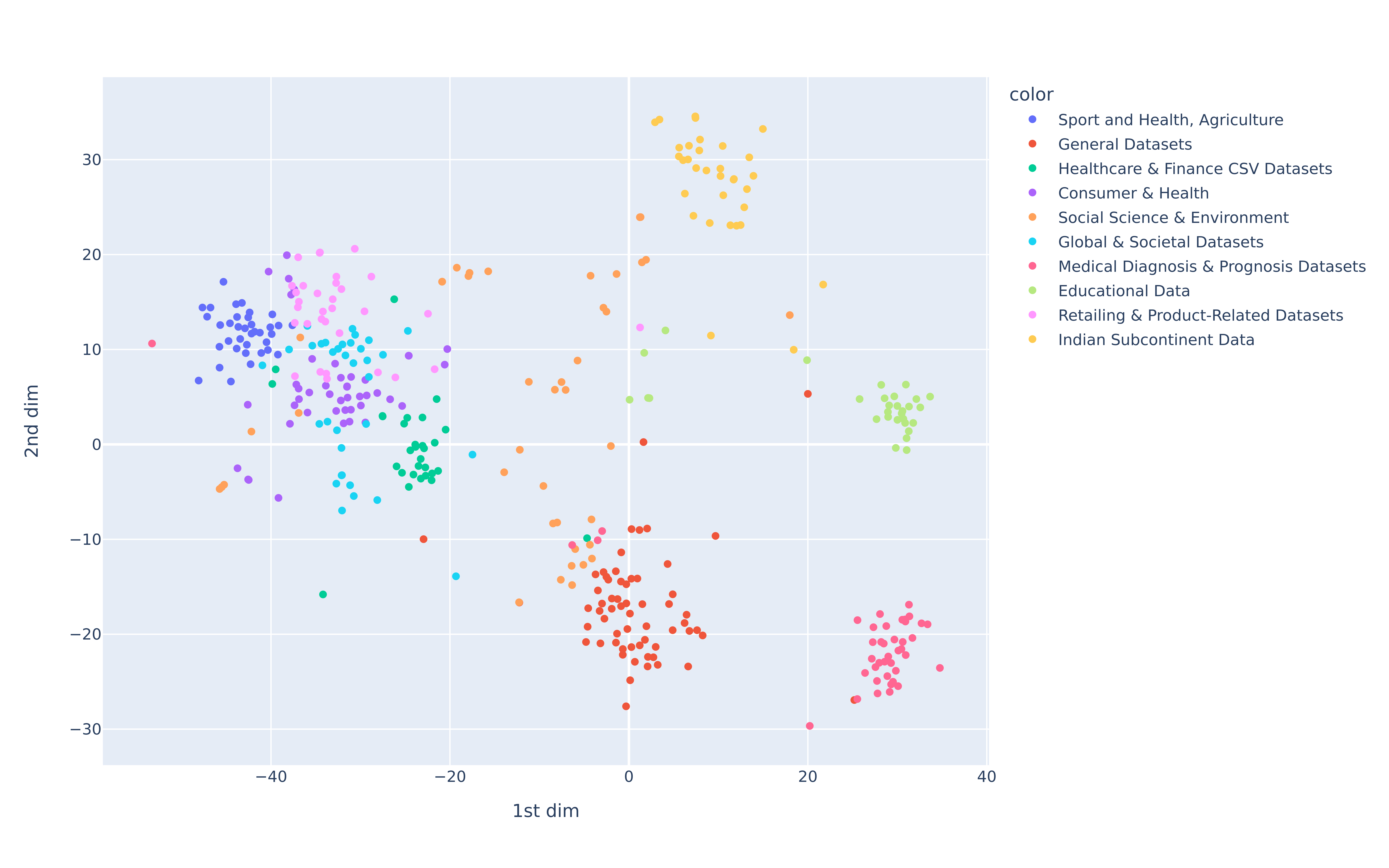
Figure 1: TSNE representation of top 10 domains clustered by $k$-means algorithm. Domain names are manually labeled by human by looking at the cluster keywords.

Table 1: Statistics about the datasets

Dataset	Raw tables	Cleaned tables train/val/test	Avg. # columns	Avg. # rows	License
Kaggle Random	43514	1148/143/144	8.37	224.8	Kaggle
Kaggle Domains	43514	969/218/248	8.37	224.8	Kaggle
GitTables	1M	1006/126/126	9.51	1112.68	CC BY 4.0

2.2 GitTables Dataset

The GitTables corpus Hulsebos et al. (2023), a large-scale collection of relational tables from CSV files on GitHub, supports the development of table representation models and applications in data management and analysis. It includes one million raw tables, many containing unstructured data like text (e.g., product reviews) or time series (e.g., server bandwidth). This requires significant data cleaning for foundational model building. After filtering for tables with only structured data, 1,258 tables remain, split into train/validation/test datasets as shown in Table 1.

3 The TabularFM Framework

TabularFM is an end-to-end framework for studying Tabular Foundational Models. In the preprocessing phase, it supports configurable data manipulation, including automated cleaning, metadata generation, and data splitting and shuffling. During training, it offers various tabular generative models with corresponding data transformation methods. For evaluation, it provides metrics to assess data synthesizer performance and transferability. Basic concepts, data transformation, experimental settings, and evaluation are briefly introduced here; detailed information is in the Appendices.

3.1 Learning Methods

Conditional Tabular GAN (CTGAN).

CTGAN, proposed by Xu et al. (2019), is a conditional GAN-based model specialized for generating tabular data. It handles mixed numerical and categorical data through datatype-specific transformations. To address mode collapse and imbalance, CTGAN employs a PacGAN-style approach Lin et al. (2018) and a training-by-sampling strategy, incorporating conditional vectors and adjusting the generator loss. It is trained using the WGAN method with gradient penalty Gulrajani et al. (2017).

Tabular Variational Autoencoder (TVAE).

While proposing CTGAN, Xu et al. (2019) also introduce a Variational Autoencoder designed for tabular data generation. The architecture mainly follow conventions and the model is optimized by using evidence lower-bound (ELBO) loss.

Shared Tabular Variational Autoencoder (STVAE).

We notice that TVAE uses a trainable parameter for standard deviations of columns, limiting dataset transferability during pretraining. To solve this, we remove this parameter and directly optimize numerical values using the ELBO loss function, naming this model Shared TVAE (STVAE).

Shared Tabular Variational Autoencoder with Metadata (STVAEM).

To enhance transferability, we add signature information to tables, which is the same for a dataset. We use embeddings of column names from a pretrained language model as this signature information and concatenate it with the input data, calling this model STVAEM.

Generation of Realistic Tabular Data (GReaT).

Transformer-based models aim to maximize the probability of predicting the next token based on previous tokens, like auto-regressive language models Jelinek (1980); Bengio et al. (2000). Thus, any pretrained generative language model can be used. GReaT Borisov et al. (2023) initializes training from large pretrained models to enhance tabular data generation through contextual representation. In this work, we use generative transformer-decoder LLM architectures Radford et al. (2018, 2019); Brown et al. (2020), specifically a distilled version of GPT, as the baseline model.

3.2 Data Transformation

Following Xu et al. (2019), we utilized one-hot encoding for the categorical columns. For each numerical column, we fitted a mixture of Gaussians with a user-defined $K$ modes. Each numerical value was normalized by subtracting the mean value and dividing by four times the standard deviation of the corresponding predicted mode. This normalization ensures that the scales of the data across tables are ignored. For transformer-based models Borisov et al. (2023), no specific data normalization is needed except converting each data value $t_{i,j}$ into a sentence of the form: column name "is" $t_{i,j}$. An example for a table with columns Age and Gender is “Age is 26 and Gender is M". For a formal definition of the data transformation process, please refer to the Appendix.

3.3 Experiment Settings

Let $\boldsymbol{\mathcal{D}}=\{\mathcal{D}_{i}\}$ represent all datasets across domains. We divide them into three types: $\boldsymbol{\mathcal{D}}^{\text{pretrain}}$ (pretraining), $\boldsymbol{\mathcal{D}}^{\text{val}}$ (validation), and $\boldsymbol{\mathcal{D}}^{\text{test}}$ (test) datasets. Our goal is to study the transferability of tabular datasets. We train a model on $\boldsymbol{\mathcal{D}}^{\text{pretrain}}$, then fine-tune it on each dataset in $\boldsymbol{\mathcal{D}}^{\text{val}}$ and $\boldsymbol{\mathcal{D}}^{\text{test}}$. Additionally, we train a separate model from scratch for each dataset. We compare the performance of fine-tuning against training from scratch.

To evaluate the performance of tabular generation, we compare the quality of synthetic data versus real data by two properties. We measure the distribution of columns data between synthetic and real data, called Column Shapes. Additionally, correlation among columns is also computed, called Column Trends. We then average the two metrics as Overall Score. As a result, we compare the performance of synthetic data to that of real data based on those metrics.

In Table 2, we summarize the statistics of the pretrained models. Due to space constraints, comprehensive information about data cleaning and preparation, hyperparameter tuning, additional details about model training and evaluation, and computing resources are thoroughly described in the Appendix.

Table 2: Statistics about the pretrained models in our work

Model	# Parameters	Dataset	Method	Split	License
ctgan_gittables	97,243,685	GitTables	CTGAN	Random	MIT
stvae_gittables	9,315,214	GitTables	STVAE	Random	MIT
great_gittables	81,912,576	GitTables	GREAT	Random	MIT
ctgan_kg_random	97,243,685	Kaggle	CTGAN	Random	Kaggle
ctgan_kg_domain	97,243,685	Kaggle	CTGAN	By domain	Kaggle
stvae_kg_random	9,315,214	Kaggle	STVAE	Random	Kaggle
stvae_kg_domain	9,315,214	Kaggle	STVAE	By domain	Kaggle
great_kg_random	81,912,576	Kaggle	GREAT	Random	Kaggle
great_kg_domain	81,912,576	Kaggle	GREAT	By domain	Kaggle

4 Benchmark Results and Discussion

In this section, we discuss experimental results using various data splits from both the Kaggle and GitTables datasets. These results are presented as standard benchmark outcomes for evaluating foundation models for tabular data. We have created corresponding leaderboards, which will be hosted on the Papers with Code platform.

4.1 Model Transferability Comparison

The results of the models on three datasets—Kaggle with random split, GitTables, and Kaggle split by domains—are presented in Table 3. All models were trained on the training subsets and validated on the test subsets, comprising 144, 126, and 248 test tables respectively. Evaluation metrics, including column shape, column pair trends, and the overall average, were averaged across all test tables. A Mann-Whitney U test was conducted to compare the distributions of results from training from scratch and pretrained models, with the null hypothesis that they are equal and the alternative hypothesis that they are not.

We present results for each learning method with and without pretraining, denoted as TVAE and TVAE Pretrained, respectively. Pretrained models of TVAE and CTGAN consistently outperform those trained from scratch by about 10 points on average. Adding meta-information did not enhance transferability, posing a future challenge of identifying optimal meta-information. Results are consistent across domain-based and random splits, with slightly worse performance in domain-based splits. These findings highlight the need for better data splitting methods to ensure maximum independence, which we plan to explore in future work.

Table 3: Transferability of pretrained models on Kaggle and GitTables dataset. The reported metrics (larger is better) and the standard deviation are shown in brackets.

Data/Split	Method	Shape	Trends	Overall	p-value
Kaggle Random	GREAT Pretrained	0.73 (0.16)	0.50 (0.25)	0.61 (0.18)	0.9
	GREAT	0.73 (0.16)	0.50 (0.25)	0.61 (0.18)
	CTGAN Pretrained	0.70 (0.16)	0.49 (0.26)	0.59 (0.19)	3.3e-8
	CTGAN	0.48 (0.17)	0.47 (0.25)	0.48 (0.17)
	TVAE Pretrained	0.47 (0.13)	0.49 (0.27)	0.48 (0.17)	0.0039
	TVAE	0.55 (0.13)	0.52 (0.26)	0.54 (0.18)
	STVAE Pretrained	0.54 (0.16)	0.45 (0.28)	0.50 (0.19)	8.5e-4
	STVAE	0.44 (0.14)	0.41 (0.28)	0.43 (0.17)
	STVAEM Pretrained	0.43 (0.17)	0.40 (0.24)	0.42 (0.16)	0.02
	STVAEM	0.35 (0.15)	0.40 (0.27)	0.37 (0.16)
GitTables	GREAT Pretrained	0.68 (0.22)	0.56 (0.27)	0.61 (0.19)	0.46
	GREAT	0.71 (0.20)	0.58 (0.25)	0.63 (0.17)
	CTGAN Pretrained	0.67 (0.12)	0.55 (0.24)	0.61 (0.14)	3.4e-5
	CTGAN	0.50 (0.18)	0.58 (0.24)	0.53 (0.15)
	TVAE Pretrained	0.45 (0.13)	0.49 (0.27)	0.47 (0.15)	0.0006
	TVAE	0.54 (0.12)	0.53 (0.27)	0.54 (0.13)
	STVAE Pretrained	0.55 (0.12)	0.59 (0.27)	0.57 (0.13)	1.2e-7
	STVAE	0.45 (0.12)	0.50 (0.27)	0.47 (0.13)
Kaggle Domain	GREAT Pretrained	0.72 (0.14)	0.56 (0.23)	0.64 (0.16)	0.7
	GREAT	0.73 (0.15)	0.56 (0.23)	0.64 (0.16)
	CTGAN Pretrained	0.69(0.12)	0.53 (0.24)	0.62 (0.15)	1.4e-14
	CTGAN	0.49 (0.16)	0.53 (0.22)	0.51 (0.14)
	TVAE Pretrained	0.39 (0.13)	0.45 (0.27)	0.42 (0.17)	9.7e-10
	TVAE	0.53 (0.13)	0.39 (0.26)	0.51 (0.18)
	STVAE Pretrained	0.48 (0.13)	0.43 (0.25)	0.46 (0.15)	0.33
	STVAE	0.42 (0.12)	0.46 (0.27)	0.44 (0.15)
	STVAEM Pretrained	0.43 (0.11)	0.39 (0.22)	0.41 (0.13)	0.02
	STVAEM	0.34 (0.13)	0.45 (0.26)	0.40 (0.14)

The results for transformer models show that transformers pretrained on textual data (GREAT) achieve the best results on the benchmark, while further pretraining with train splits containing tabular data (GREAT Pretrained) slightly decreases performance. There are a few potential reasons behind this behavior. First, methods such as CTGAN and TVAE are not column permutation invariant, whereas the attention mechanism adopted in transformers is, allowing for more effective representation learning. Second, transformers are based on GPT-2, which was trained on a larger corpus of textual data. Even though GPT-2 was not trained on tabular data, it has acquired general knowledge that can be transferred to tabular data. Therefore, a future challenge is to create larger training tabular datasets to pretrain transformers in a way that outperforms current text-based models.

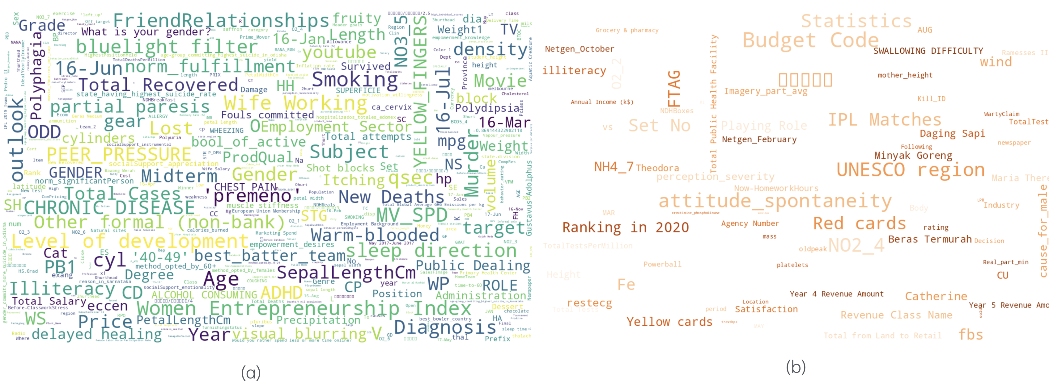
Figure 2: Wordclouds demonstrate columns with high transferability (a) and low transferability (b).

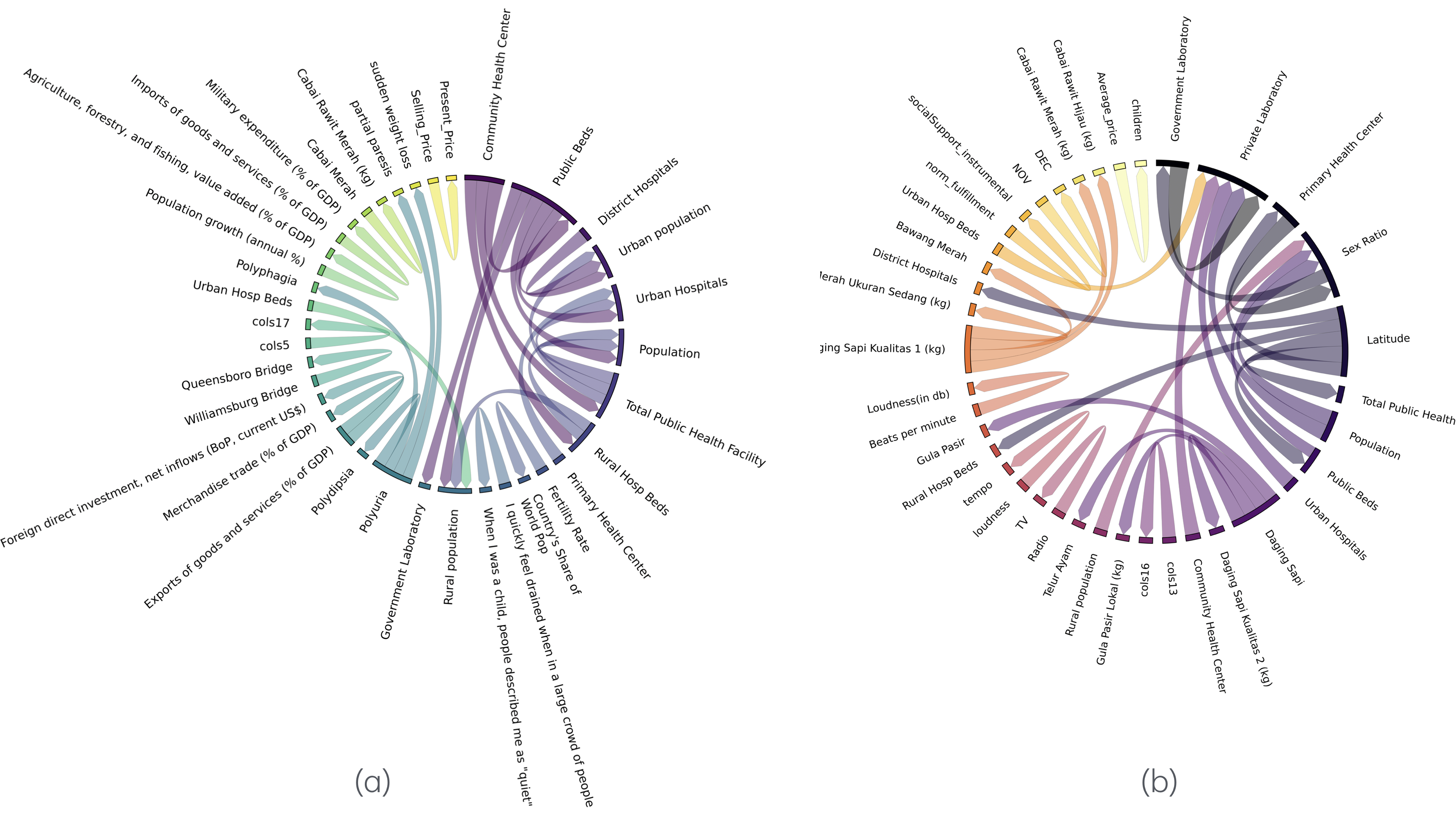
Figure 3: The plots illustrate the column pairs with the most significant differences between the pair trends of the pretrained models and the model trained from scratch in (a), and vice versa in (b).

4.2 Transferability Analysis

To understand the key factors driving the transferability results discussed in the previous section, we conducted further analysis. This analysis illuminates the types of knowledge that pretrained models can and cannot transfer. Figure 2 presents wordclouds of the column names, where the size of each word corresponds to the absolute value of the difference between the performance of the pretrained models and the model trained from scratch. Figure 2.a displays columns where the pretrained models outperform the models trained from scratch, while Figure 2.b shows the opposite. We observe that highly general knowledge such as Age, Gender, Chronic Disease is transferable, whereas specific knowledge such as Unesco region, Budget Code, Red Cards is not, which is logical.

To understand how pretrained models utilize general correlation patterns in data and transfer that knowledge across datasets, Figure 3 illustrates the links between columns where the difference between the pair trends of the pretrained models and the models trained from scratch is highest (Figure 3.a) and vice versa (Figure 3.b). We observe that general knowledge about the correlation between hospital beds and urban population or the link between weight loss and polydipsia via polyuria transfers well through pretraining. This finding is noteworthy because the models were pretrained solely by observing the data distribution, yet they could detect and transfer meaningful correlated patterns across datasets. Our analysis confirms that, despite tabular data being noisier than other types of data, specific types of knowledge can be transferred across data. Thus, developing foundational models for tabular data is a promising research direction.

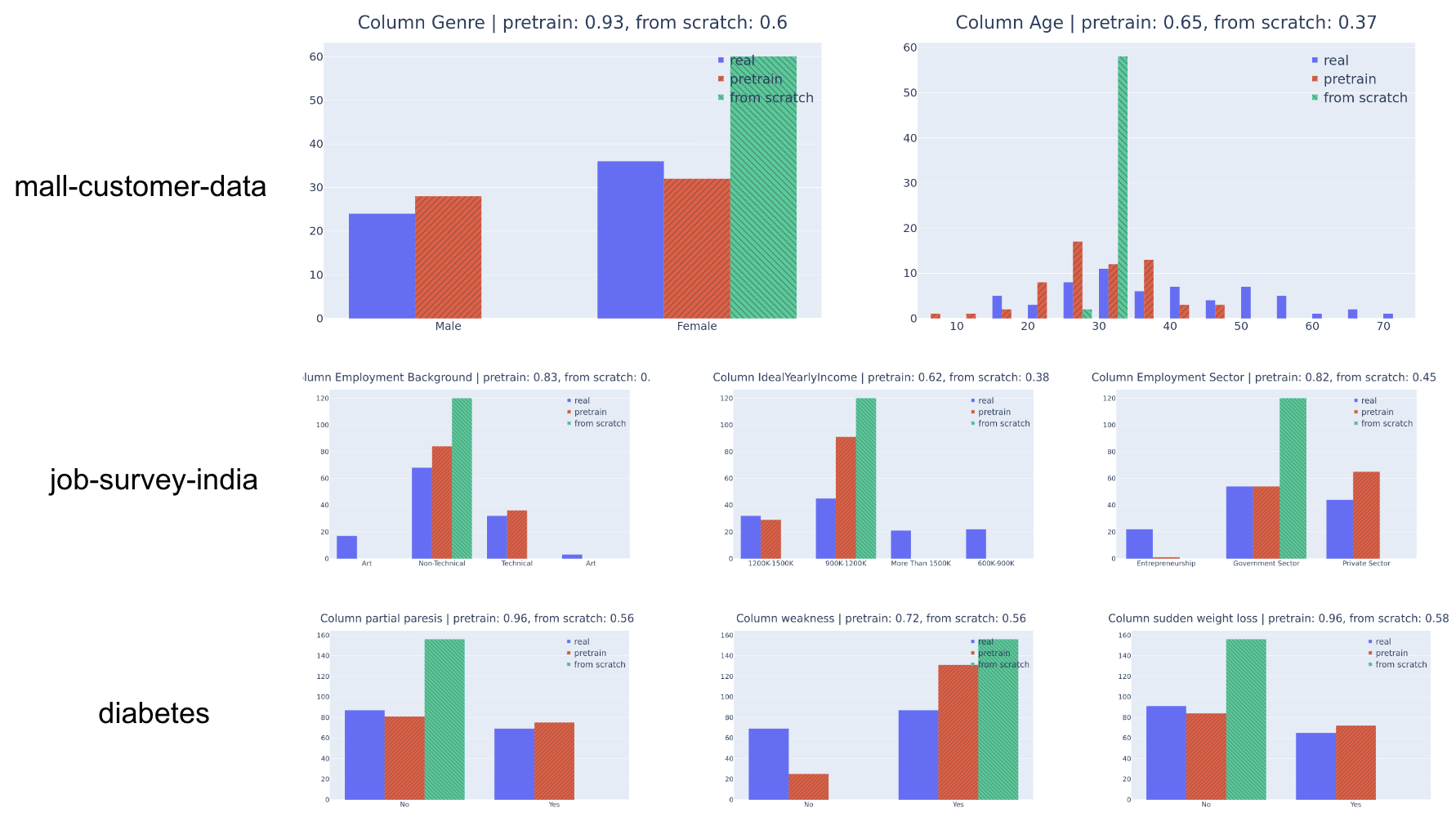
Figure 4: Column shape comparison of STVAE Pretrained prediction and STVAE from scratch.

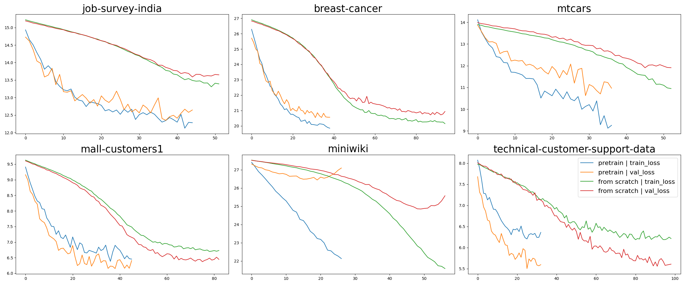
Figure 5: Training and validation loss of STVAE models when they are pretrained versus trained from scratch. Pretrained STVAE converge faster toward more optimal solutions.

In Figure 4, the histogram compares synthesized data with ground truth data. It reveals that the STVAE trained from scratch primarily predicts the mode of the column, neglecting the distribution tails. In contrast, the pretrained STVAE effectively captures the tails of the distribution. This difference is reflected in the faster learning curve shown in Figure 5, where the benefits of pretraining include quicker and better convergence. These findings are promising and confirm that transferability between tabular datasets is feasible.

5 Related Work

Learning representation for tabular data has seen significant advancements with various approaches aiming to enhance performance, interpretability, and efficiency.

Generative Adversarial Network-based methods: Generative adversarial networks (GANs) have been explored for tabular data with models like TGAN (Xu and Veeramachaneni, 2018) and CTGAN (Xu et al., 2019). TGAN focuses on generating high-quality synthetic tables with mixed discrete and continuous variables, while CTGAN uses conditional GANs to address the challenges of modeling imbalanced and multi-modal tabular data. Both models demonstrate the potential of GANs to generate realistic synthetic tabular data, facilitating privacy-preserving data generation and enhancing data availability for training robust machine learning models.

Distribution-agnostic Deep Learning Approaches: (Joffe, 2021) proposes a CNN-based architecture for transferring patterns from tabular data by treating it as a 2D image, with a min-max scaling method for numerical columns to address scaling issues. The CNN learns spatial relations between columns, but since column order doesn’t matter in tabular data, random shuffling of columns during training is required. (Iida et al., 2021) introduces TABBIE, which uses two transformers to independently encode rows and columns, pooling their representations at each layer. Like training BERT by masking a random word, it corrupts a random cell in the input table and trains the model to predict the corrupted cells. This approach ignores the challenges associated with tabular data, such as numeric and categorical data normalization and column order invariance. TURL in (Deng et al., 2021) considers entity embedding using a transformer encoder for relational web tables. Each entity is represented with properties, and the data is kept in a relational web-table format. Similar to TABBIE, TURL first serializes the tables into sequences and then trains the transformer-based model with a masking objective similar to training BERT. The proposed method only works for clean data and cannot learn important patterns beyond the clean dataset used in the experiments. UNITABE (Yang et al., 2024) consists of a transformer encoder and a shallow LSTM decoder to leverage the relationship between column names and values. To handle varying data types, the authors propose a feature processor that considers each cell in a table as a key-value pair, representing the column name and the corresponding column value. The work (Arik and Pfister, 2021) proposes TabNet – a deep learning architecture for tabular data that uses sequential attention to select features at each decision step. This approach enables both local and global interpretability, as well as efficient learning by focusing on the most salient features. Its ability to handle raw tabular data without preprocessing and its application of unsupervised pretraining for improved performance show its strengths in handling diverse tabular datasets with high interpretability. Moreover, the paper (Nam et al., 2023) proposes STUNT to improve performance in few-shot learning scenarios. STUNT applies meta-learning to generalize knowledge from these self-generated tasks by generating pseudo-labels from unlabeled data through $k$-means clustering of randomly chosen column subsets. TabPFN (Hollmann et al., 2022) is a transformer-based model that solves supervised classification problems on small tabular datasets without hyperparameter tuning. This approach highlights the potential of pretrained models for efficient and accurate tabular data classification, setting a precedent for rapid and effective tabular data processing. TransTab (Wang and Sun, 2022) is a method for learning transferable representations across tables with varying structures. TransTab allows pretraining on multiple distinct tables and fine-tuning on target datasets by converting table rows into generalizable embedding vectors and employing a gated transformer model that integrates column descriptions and cell values. This approach addresses the challenge of maintaining model performance across tables with different columns and structures, showing the versatility of transformer-based models for tabular data. Furthermore, the work (Padhi et al., 2021) extends the application of transformers to tabular time series data. They demonstrated on both synthetic and real-world datasets by leveraging hierarchical structures of these models in tabular time series data to improve performance in downstream tasks like classification and regression. This work highlights the adaptability of transformer models to various tabular data formats, including time series.

Pretrained Large Language Model Adaptation: Several authors propose methods to adapt pretrained large language models, such as LLaMA and GPT, to tabular data (Zhang et al., 2023; Hegselmann et al., 2023). Using LLaMA, TabFM in (Zhang et al., 2023) is trained with 115 public datasets by employing generative modeling of rows encoded as text along with task and column descriptions, incorporating additional loss for feature reconstruction. TabLLM in (Hegselmann et al., 2023) fine-tunes the T0 model by transforming a table into a natural text representation using serialization methods. LIFT (Dinh et al., 2022) is a language-interfaced fine-tuning method that fine-tunes GPT-based architectures by converting labeled samples into sentences with a fixed template then fine-tuning LLMs with sentence datasets.

All these approaches collectively highlight the advancements in leveraging transformer models and GANs for tabular data. Our framework, TabularFM, builds upon these foundations by introducing state-of-the-art methods tailored specifically for tabular data, including GANs, VAEs, and Transformers. By using an extensive collection of cleaned tabular datasets and offering pretrained models along with benchmarking tools, TabularFM aims to advance the field significantly, providing a comprehensive solution for developing and evaluating foundational models for tabular data.

6 Limitations, Conclusions and Future Work

In this work, we have preprocessed and curated about a million of tables to build and benchmark tabular foundation models. Our comparative study and detailed analysis of the benchmark results demonstrate the advantages of pretraining, providing insights into how pretraining transfers general knowledge across tabular datasets. These findings confirm the potential applications of tabular FMs. However, the challenges in building effective tabular FMs remain an open question. Our work offers a framework for rapidly benchmarking new models in the future.

Our study is limited to three types of neural learning architectures and focuses on numerical and categorical data. For future work, we plan to extend our framework to encompass a more diverse range of data types stored in tabular format and to train larger models on more extensive datasets.

Appendix A Released Pretrained Models

We have released all the pretrained models for the GitTables datasets under the MIT license on Huggingface. For the models trained on Kaggle datasets, we offer the datasets and detailed documentation on the training steps, as some Kaggle tables have restricted licenses. A summary of the models’ statistics can be found in Table 4. By offering these pretrained models, we enable researchers and practitioners to utilize state-of-the-art techniques without the need for extensive computational resources or time-consuming training processes.

Table 4: Statistics about the pretrained models in our work

Model	# Parameters	Dataset	Method	Split	License
ctgan_gittables	97,243,685	GitTables	CTGAN	Random	MIT
stvae_gittables	9,315,214	GitTables	STVAE	Random	MIT
great_gittables	81,912,576	GitTables	GREAT	Random	MIT
ctgan_kg_random	97,243,685	Kaggle	CTGAN	Random	Kaggle
ctgan_kg_domain	97,243,685	Kaggle	CTGAN	By domain	Kaggle
stvae_kg_random	9,315,214	Kaggle	STVAE	Random	Kaggle
stvae_kg_domain	9,315,214	Kaggle	STVAE	By domain	Kaggle
great_kg_random	81,912,576	Kaggle	GREAT	Random	Kaggle
great_kg_domain	81,912,576	Kaggle	GREAT	By domain	Kaggle

Appendix B Hyperparameter Sensitivity Analysis and Settings

The hyperparameters used in our experiments are summarized in Table LABEL:tab:hpo. To determine the optimal network size and learning rate for CTGAN and TVAE, we conducted pretraining with learning rates of 1e-3, 1e-4, 1e-5 and network sizes set to either small or normal ones. The performance results of the CTGAN model on the validation random split of the Kaggle dataset, showing the effects of varying network size and learning rate, are presented in Figure 8 and Figure 9 respectively. With different network sizes and learning rates, the performance of the pretrained model consistently surpassed that of models trained from scratch. Besides, when the model size is reduced, there is a slight decline in performance compared to larger models. Thus, increasing the model size is a potential strategy to further enhance results. For GREAT, we used the recommended default network and learning rate.

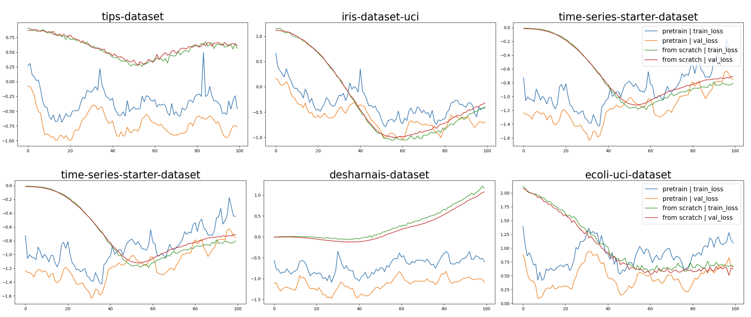
Figure 6: Training and validation loss of the generator of the CTGAN models when they are pretrained and finetuned on the data versus trained from scratch.

Appendix C Computing Resource

We conducted all the experiments on a machine equipped with 4 CPUs, 50GB of memory, and one A100 GPU. Each pretraining task was configured to run for a maximum of 2 days or 500 epochs, whichever was reached first. Fine-tuning and training from scratch require less computing power and typically complete within 24 hours.

Appendix D Transferability Results Analysis

In this section, we discuss additional analysis on transferability. Figure 6 illustrates the training and validation loss of the generator of the CTGAN models when they are pretrained and finetuned on the data versus trained from scratch. We can see the pretrained generators provide much better initial prediction and tends to converge faster to better solutions.

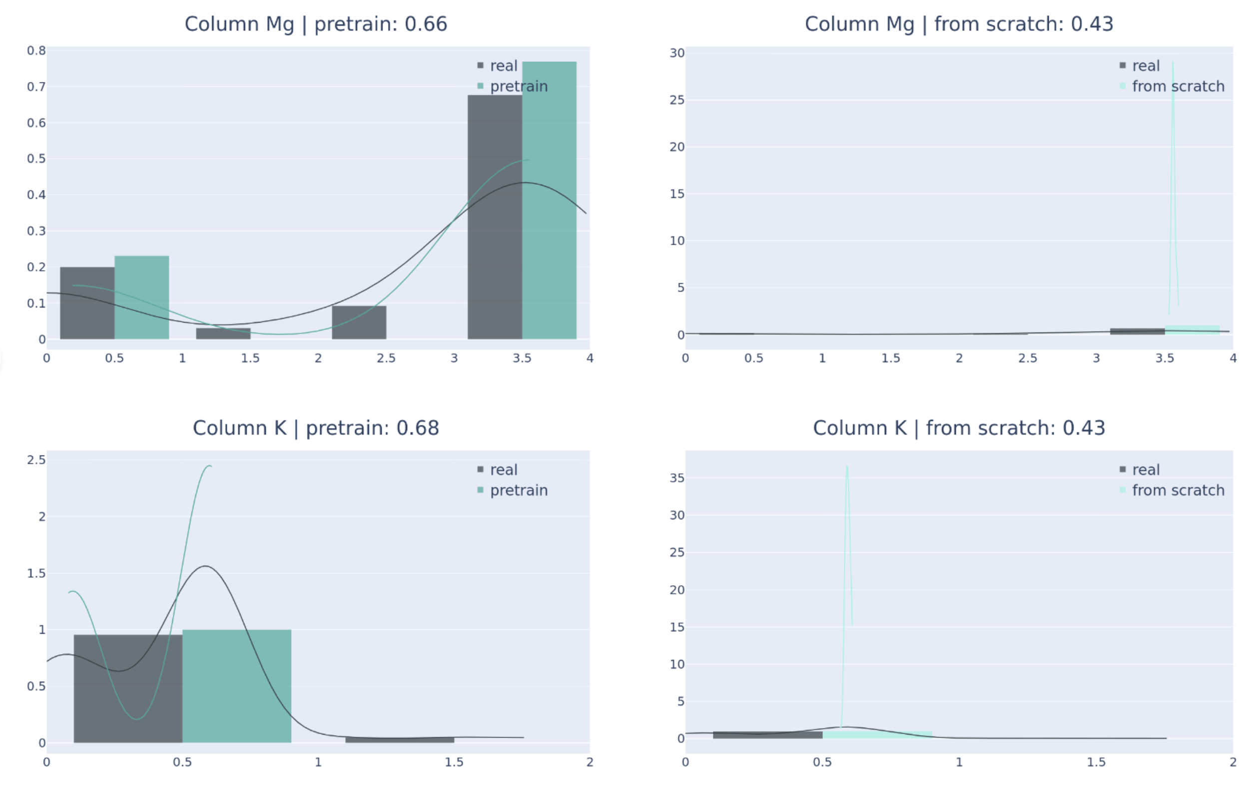
Figure 7: Column shape of pre-trained STVAE models and STAVE models trained from scratch for the table composition of glass.

Figure 7 illustrates the performance of pre-trained STVAE models compared to STVAE models trained from scratch for the table composition of glass. The distribution predicted by the pre-trained models closely aligns with the ground truth data for each column. In contrast, the STVAE models trained from scratch tend to overfit to the mode of the distribution, likely due to the limited data available.

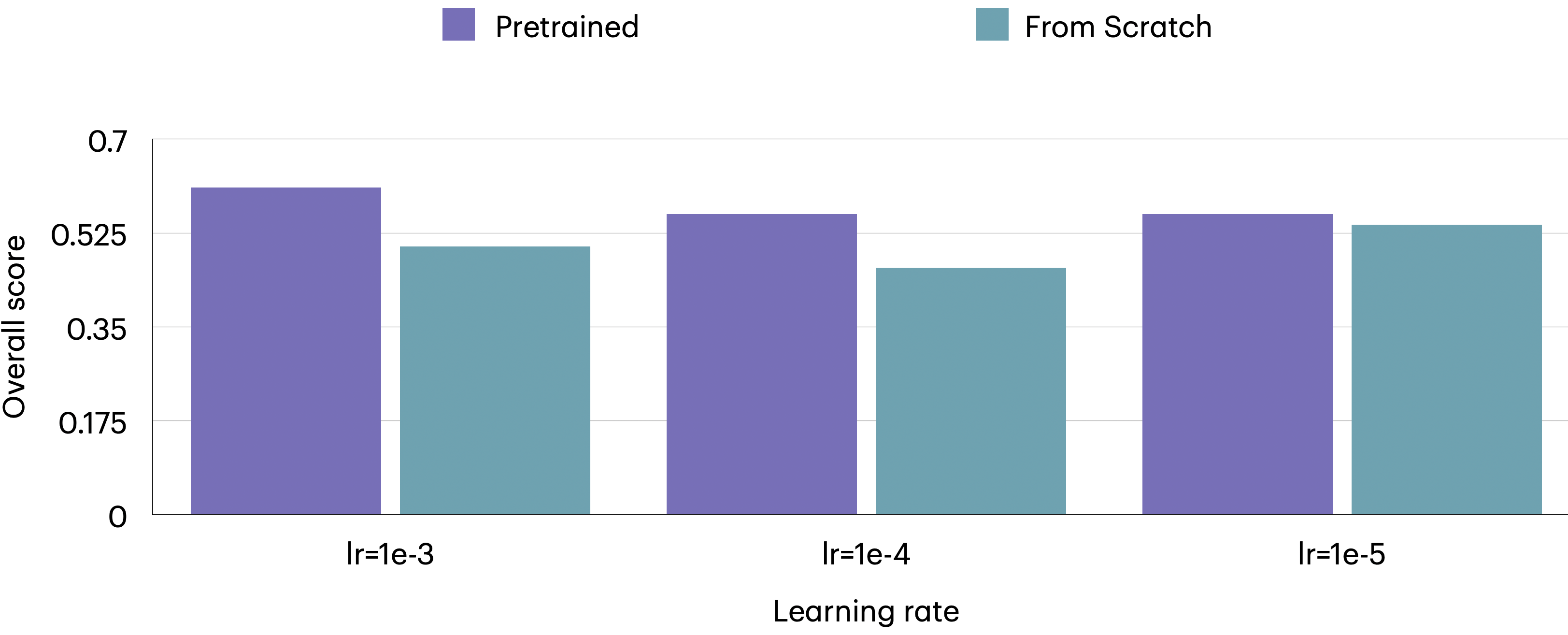
Figure 8: The impact of learning rate on the results of CTGAN with pretraining and training from scratch, the results were calculated on the validation tables of the random split of the Kaggle dataset.

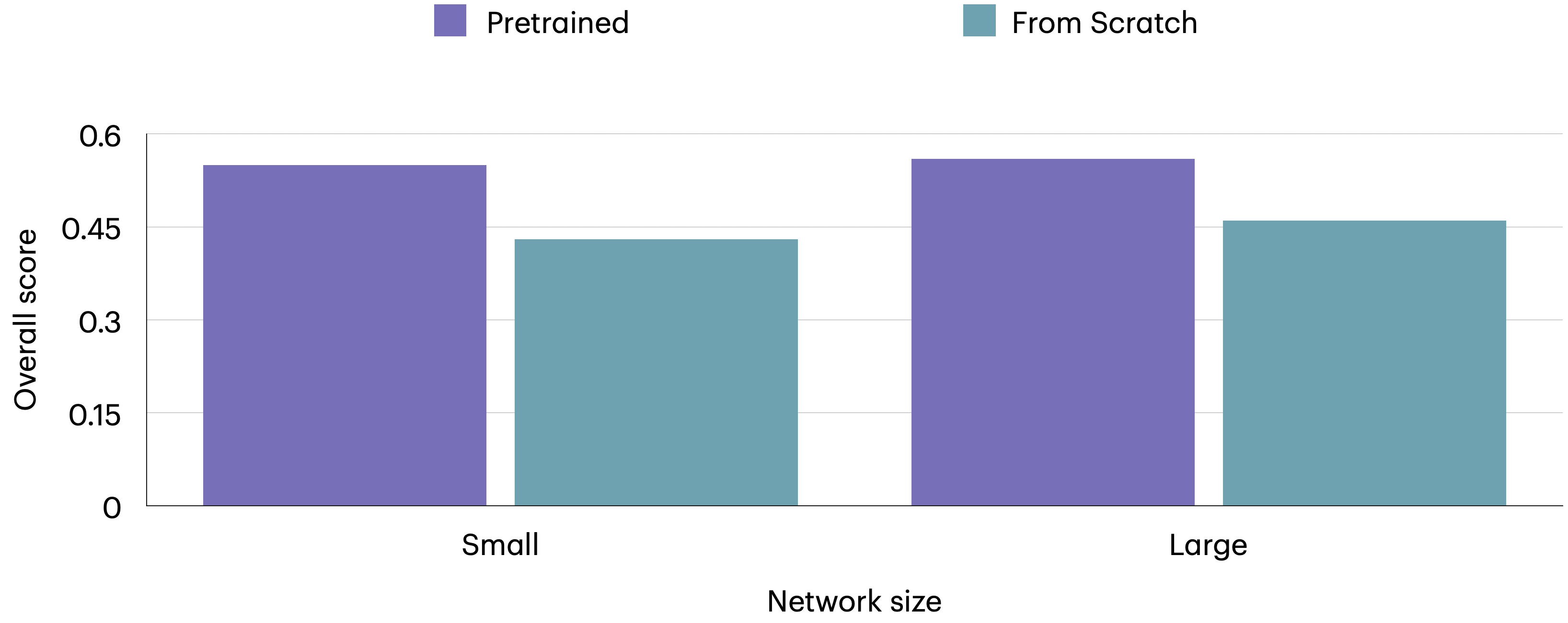
Figure 9: The impact of network size on the results of CTGAN with pretraining and training from scratch, the results were calculated on the validation tables of the random split of the Kaggle dataset.

Appendix E Supported Learning Methods

We briefly describe the technical details of the learning methods used in this paper.

E.1 Conditional Tabular GAN (CTGAN).

CTGAN is a conditional GAN-based model for tabular data proposed by Xu et al. [2019]. Particularly, a table row $\mathbf{r}$ in the dataset $\mathcal{D}$, i.e. $\mathbf{r}\in\mathcal{D}\sim\mathbb{P}$ where $\mathbb{P}$ is the distribution of real dataset $\mathcal{D}$. To generate a synthetic data $\hat{\mathbf{r}}$, a generator $\mathcal{G}(\mathbf{z})$, where $\mathbf{z}\sim\mathcal{N}(\mathbf{0},\mathbf{1})$ is learned, formally.

$$\hat{\mathbf{r}}\sim\mathbb{P}_{\mathcal{G}}(\mathbf{z})$$ (1)

In the setting of conventional GAN, to valdiate the performance of the generator, a discriminator, or a critic score $\mathcal{C}$ is leveraged.

$$\mathcal{C}(\mathbb{P},\mathbb{P}_{\mathcal{G}})$$ (2)

However, GAN may encounter mode collapse in case of imbalance datasets. To address this problem, CTGAN add a condition to make the synthetic data attached to a pre-defined category. Particularly, a specific category $k^{*}\in D_{i}$ is appointed during the generation, thus

$$\hat{\mathbf{r}}\sim\mathbb{P}_{\mathcal{G}}(\mathbf{z}|D_{i}=k^{*})$$ (3)

To accomplish this, CTGAN modelled the condition in (3) as conditional vector, i.e. cond and modify the generator loss to optimize it. Furthermore, training-by-sampling strategy is proposed to optimize CTGAN.

Conditional vector.

All categorical columns $D_{1},D_{2},\dots,D_{N_{d}}$ are leveraged to initiate conditional vectors. Suppose that a specific categorical value $k^{*}$ is chosen from a categorical column $D_{i^{*}}$, a one-hot vector $\mathbf{m}_{i}=[m_{i}^{(k)}],k=1,\dots,|D_{i}|$ is obtained as the mask, which is described as

$$m_{i}^{(k)}=\begin{cases}1,&\text{if}\ i=i^{*}\text{and}k=k^{*}\\ 0,&\text{otherwise}\end{cases}$$ (4)

Hence, a conditional vector $cond$ is represented as

$$cond=\mathbf{m}_{1}\oplus\mathbf{m}_{2}\oplus\dots\oplus\mathbf{m}_{N_{d}}$$ (5)

Generator loss.

It is obvious that conditional vector should be leveraged in the optimization. In fact, each mask one-hot vector $\mathbf{m}_{i}$ is constrained the generated data $\hat{\mathbf{d}}_{i}\in D_{i}$ to enforce it following the given condition. Hence, a cross-entropy loss between $\mathbf{m}_{i}$ and $\hat{\mathbf{d}}_{i}$ is supplemented into the existing generator loss of CTGAN to optimize the conditional vectors.

Training-by-sampling strategy.

We further clarify the sampling strategy with the involvement of conditional vectors to help optimizing the discriminator as follows

1. Initiate original masked conditional vectors: setup all $\mathbf{m}_{i}=[m_{i}^{(k}]_{k=1,2,\dots,|D_{i}|},i=1,2,\dots,N_{d}$.

2. Randomly select a target categorical column: let $i^{*}$ be the index of chosen categorical column, $D_{i^{*}}$ is sampled with equal probability.

3. Sample a target category of the selected categorical column: construct PMF over all categories of $D_{i^{*}}$ and randomly select a category $k^{*}\in D_{i^{*}}$.

4. Adjust conditional vectors: modify the value $\mathbf{m}_{i^{*}}^{(k^{*})}=1$

5. Finalize the conditional vectors: concatenate all masked vectors, $cond=\mathbf{m}_{1}\oplus\mathbf{m}_{2}\oplus\dots\oplus\mathbf{m}_{N_{d}}$

Algorithm 1 describes training by batch procedure of CTGAN. The model are trained using the gradient penalty manner of WGAN Gulrajani et al. [2017] and is further leveraged the PacGAN style to get rid of mode collapse Lin et al. [2018].

Algorithm 1 Training CTGAN by batch

Input: Dataset $\mathcal{D}$ with $\mathbf{T}_{train}$ transformed data, Generator $\mathcal{G}$ with paramters $\Phi_{\mathcal{G}}$, Critic $\mathcal{C}$ with parameters $\Phi_{\mathcal{C}}$, Optimizer $\mathcal{O}$ with learning rate $\eta$
Output:

1:Initiate masks $\{[\mathbf{m}_{i}]_{i=1,\dots,N_{d}}\}_{j}$,   for $1\leq j\leq batch$

2:Create conditional vectors $\{cond_{j}\}$,   for $1\leq j\leq batch$

3:Sample $\{z_{j}\}\sim\mathcal{N}(0,\mathbf{I})$,   for $1\leq j\leq batch$

4:

5:Generate $\hat{\mathbf{r}}_{j}\leftarrow\mathcal{G}(z_{j},cond_{j})$,   for $1\leq j\leq batch$ $\triangleright$ Generate synthetic data

6:Sample $\mathbf{r}_{j}\sim\text{Uniform}(\mathbf{T}_{train}|cond_{j})$,   for $1\leq j\leq batch$ $\triangleright$ Sample real data

7:

8:$cond_{k}^{(pac)}\leftarrow cond_{k\times pac+1}\oplus\dots\oplus cond_{k\times pac+pac}$, for $1\leq k\leq batch/pac$ $\triangleright$ Pac conditional vector

9:$\hat{\mathbf{r}}_{k}^{(pac)}\leftarrow\hat{\mathbf{r}}_{k\times pac+1}\oplus\dots\oplus\hat{\mathbf{r}}_{k\times pac+pac}$, for $1\leq k\leq batch/pac$ $\triangleright$ Pac synthetic data

10:$\mathbf{r}_{k}^{(pac)}\leftarrow\mathbf{r}_{k\times pac+1}\oplus\dots\oplus\mathbf{r}_{k\times pac+pac}$, for $1\leq k\leq batch/pac$ $\triangleright$ Pac real data

11:

12:$\mathcal{L}_{\mathcal{C}}\leftarrow\frac{1}{batch/pac}\sum_{k\in batch/pac}\left(\mathcal{C}(\hat{\mathbf{r}}_{k}^{(pac)},cond_{k}^{(pac)})-\mathcal{C}(\mathbf{r}_{k}^{(pac)},cond_{k}^{(pac)})\right)$ $\triangleright$ Calculate critic loss

13:

14:Sample $\rho_{1}\dots\rho_{batch/pac}\sim\text{Uniform}(0,1)$

15:${\mathbf{r}}_{k}^{(pac)}\leftarrow\rho_{k}\hat{\mathbf{r}}_{k}^{(pac)+(1-\rho_{k})\mathbf{r}_{k}^{(pac)}}$,   for $1\leq k\leq batch/pac$

16:$\mathcal{L}_{GP}\leftarrow\frac{1}{batch/pac}\sum_{k\in batch/pac}\left(||\Delta_{\tilde{\mathbf{r}}_{k}^{(pac)}}\mathcal{C}(\tilde{\mathbf{r}}_{k}^{(pac)},cond_{k}^{(pac))}||_{2}-1\right)^{2}$ $\triangleright$ Gradient penalty

17:Update gradient $\Phi_{\mathcal{C}}$ with $\mathcal{O}$ and $\eta$

18:

19:Generate $\hat{\mathbf{r}}_{j}$ following lines 1 to 8.

20:$\mathcal{L}_{\mathcal{G}}\leftarrow-\frac{1}{batch/pac}\sum_{k\in batch/pac}\mathcal{C}(\hat{\mathbf{r}}_{k}^{(pac)},cond_{k}^{(pac)})+\frac{1}{batch}\sum_{j\in batch}\mathbb{CE}(\hat{\mathbf{d}}_{i^{*},j},\mathbf{m}_{i^{*}})$

21:Update gradient $\Phi_{\mathcal{G}}$ with $\mathcal{O}$ and $\eta$

E.1.1 Architecture

We denote $L$ as hidden dimension of fully connected layers in the architecture, $L_{l}$ represents the output dimension of that layer.

The generator architecture $\mathcal{G}(\mathbf{z},\textit{cond})$ is formally described as

$$~{}\left\{\begin{array}[]{@{}l@{}l@{}}\textbf{h}_{0}=\mathbf{z}\oplus\textit{cond}\\[10.00002pt] \textbf{h}_{1}=\textbf{h}_{0}\oplus\text{ReLU}(\text{BN}(\text{FC}_{|\mathbf{h}_{0}|\rightarrow L_{0}}(\textbf{h}_{0})))\\[10.00002pt] \textbf{h}_{l+1}=\textbf{h}_{l}\oplus\text{ReLU}(\text{BN}(\text{FC}_{|\mathbf{h}_{l}|\rightarrow L_{l}}(\textbf{h}_{l})))&\qquad 1\leq l\leq L\\[10.00002pt] \hat{\alpha}_{i}=\tanh(\text{FC}_{|\mathbf{h}_{L}|\rightarrow 1}(\textbf{h}_{L}))&\qquad 1\leq i\leq N_{c}\\[10.00002pt] \hat{\boldsymbol{\beta}}_{i}=\text{gumbel}_{0.2}(\text{FC}_{|\mathbf{h}_{L}|\rightarrow m_{i}}(\textbf{h}_{L}))&\qquad 1\leq i\leq N_{c}\\[10.00002pt] \hat{\mathbf{d}}_{i}=\text{gumbel}_{0.2}(\text{FC}_{|\mathbf{h}_{L}|\rightarrow|D_{i}|}(\textbf{h}_{L}))&\qquad 1\leq i\leq N_{d}\end{array}\right.$$

and the architecture of critic $\mathcal{C}$ is defined as

$$~{}\left\{\begin{array}[]{@{}l@{}l@{}}\textbf{h}_{0}=N_{\text{pac}}\times(\mathbf{r}_{k}\oplus\textit{cond}_{k})\\[10.00002pt] \textbf{h}_{1}=\text{drop}(\text{leaky}_{0.2}(\text{FC}_{|\mathbf{h}_{0}|\rightarrow L_{0}}(\mathbf{h}_{0}))\\[10.00002pt] \textbf{h}_{l+1}=\text{drop}(\text{leaky}(\text{FC}_{|\mathbf{h}_{l}|\rightarrow L_{l}}(\mathbf{h}_{l}))&\qquad 1\leq l\leq L\\[10.00002pt] \mathcal{C}=\text{FC}_{|\mathbf{h}_{L}|\rightarrow 1}(\mathbf{h}_{L})\end{array}\right.$$

E.2 Tabular Variational Autoencoder (TVAE).

While proposing CTGAN, the authors also introduce a Variational Autoencoder designed for tabular data generation. Let $q_{\phi}(\mathbf{z}_{j}|\mathbf{r}_{j})$ and $p_{\theta}(\mathbf{r}_{j}|\mathbf{z}_{j})$ are the encoder and decoder following the settings of variational autoencoder, respectively. An evidence lower-bound (ELBO) loss is induced to optimize the model as follow

$$\log p_{\theta}(\mathbf{r}_{j})\geq\mathop{\mathbb{E}_{q_{\phi}(\mathbf{z}_{j}|\mathbf{r}_{j})}}\left[\log p_{\theta}(\mathbf{r}_{j}|\mathbf{z}_{j})\right]-\mathbb{KL}\left[q_{\phi}(\mathbf{z}_{j}|\mathbf{r}_{j})||p(\mathbf{z}_{j})\right]$$ (6)

Instead of directly calculating numerical value $\hat{c}_{i,j}$ in synthetic data $\hat{\mathbf{r}}_{j}$ generated from $p_{\theta}(\mathbf{r}_{j}|\mathbf{z}_{j})$, the authors proposed to sample it from an intermediate distribution, $\hat{c}_{i,j}\sim\mathcal{N}(\bar{\alpha}_{i,j},\delta_{j})$, where $\delta_{j}$ is the additional learnable parameter representing the standard deviation of a numerical column $C_{j}$. As a result, the likelihood function is formally described as follow, with $\mathbb{CE}$ denotes the cross-entropy loss function

$$\log p_{\theta}(\mathbf{r}_{j}|\mathbf{z}_{j})=\sum_{i}^{N_{c}}\log\frac{1}{\sqrt{2\pi\sigma}}\exp{\frac{\alpha_{i,j}-\bar{\alpha}_{i,j}}{2\pi\sigma^{2}}}+\sum_{i}^{N_{c}}\mathbb{CE}\left(\hat{\boldsymbol{\beta}}_{i,j},\boldsymbol{\beta}_{i,j}\right)+\sum_{i}^{N_{d}}\mathbb{CE}\left(\hat{\mathbf{d}}_{i,j},\mathbf{d}_{i,j}\right)$$ (7)

E.2.1 Architecture

The encoder architecture is

$$~{}\left\{\begin{array}[]{@{}l@{}l@{}}\textbf{h}_{0}=\text{ReLU}(\text{FC}_{|\mathbf{r}_{j}|\rightarrow L_{0}}(\mathbf{r}_{j}))\\[10.00002pt] \textbf{h}_{1}=\text{ReLU}(\text{FC}_{|\mathbf{h}_{0}|\rightarrow L_{1}}(\mathbf{h}_{0}))\\[10.00002pt] \textbf{h}_{l+1}=\text{ReLU}(\text{FC}_{|\mathbf{h}_{l}|\rightarrow L_{l+1}}(\mathbf{h}_{l}))&\qquad 1\leq l\leq L\\[10.00002pt] \mathbf{\mu}=\text{FC}_{|\mathbf{h}_{L}|\rightarrow L}(\mathbf{h}_{L})\\[10.00002pt] \mathbf{\sigma}=\exp(\frac{1}{2}\text{FC}_{|\mathbf{h}_{L}|\rightarrow L}(\mathbf{h}_{L}))\\[10.00002pt] q_{\phi}(z_{j}|\mathbf{r}_{j})\sim\mathcal{N}(\mu,\sigma\mathbf{I})\end{array}\right.$$

The decoder architecture is

$$~{}\left\{\begin{array}[]{@{}l@{}l@{}}\textbf{h}_{0}=\text{ReLU}(\text{FC}_{L_{0}\rightarrow L_{1}}(\mathbf{z}_{j}))\\[10.00002pt] \textbf{h}_{l}=\text{ReLU}(\text{FC}_{|\mathbf{h}_{l}|\rightarrow L_{l+1}}(\mathbf{h}_{l-1}))&1\leq l\leq L\\[10.00002pt] \bar{\alpha}_{i,j}=\tanh(FC_{|\mathbf{h}_{L}|\rightarrow 1}(\mathbf{h}_{L}))\\[10.00002pt] \hat{\alpha}_{i,j}\sim\mathcal{N}(\bar{\alpha}_{i,j},\delta_{i})&1\leq i\leq N_{c}\\[10.00002pt] \hat{\boldsymbol{\beta}}_{i,j}\sim\text{softmax}(\text{FC}_{128\rightarrow m_{i}}(\mathbf{h}_{2}))&1\leq i\leq N_{c}\\[10.00002pt] \hat{\mathbf{d}}_{i,j}\sim\text{softmax}(\text{FC}_{128\rightarrow|D_{i}|}(\mathbf{h}_{2}))&1\leq i\leq N_{d}\\[10.00002pt] p_{\theta}(\mathbf{r}_{j}|z_{j})=\prod_{i=1}^{N_{c}}\mathbb{P}(\hat{\alpha}_{i,j}=\alpha_{i,j})\prod_{i=1}^{N_{c}}\mathbb{P}(\hat{\boldsymbol{\beta}}_{i,j}=\boldsymbol{\beta}_{i,j})\prod_{i=1}^{N_{d}}\mathbb{P}(\hat{\alpha}_{i,j}=\alpha_{i,j})\end{array}\right.$$

E.3 Shared Tabular Variational Autoencoder (STVAE).

We observe that column standard deviation $\delta_{i}$ in TVAE prevents the transferability across datasets during the pretraining since each dataset deserves a corresponding set of standard deviation for its numerical columns. To address the problem, we omit this parameter and directly optimize generated numerical value $\hat{\alpha}_{i,j}$ in the likelihood function using mean squared error. Hence, we refer this model as Shared TVAE (STVAE), and the modified version of $\log p_{\theta}(\mathbf{r}_{j}|\mathbf{z}_{j})$ is defined as

$$\log p_{\theta}(\mathbf{r}_{j}|\mathbf{z}_{j})=\sum_{i}^{N_{c}}\mathbb{MSE}\left(\hat{\alpha}_{i,j},\alpha_{i,j}\right)+\sum_{i}^{N_{c}}\mathbb{CE}\left(\hat{\boldsymbol{\beta}}_{i,j},\boldsymbol{\beta}_{i,j}\right)+\sum_{i}^{N_{d}}\mathbb{CE}\left(\hat{\mathbf{d}}_{i,j},\mathbf{d}_{i,j}\right)$$ (8)

E.3.1 Architecture

The decoder architecture is

$$~{}\left\{\begin{array}[]{@{}l@{}l@{}}\textbf{h}_{0}=\text{ReLU}(\text{FC}_{L_{0}\rightarrow L_{1}}(\mathbf{z}_{j}))\\[10.00002pt] \textbf{h}_{l}=\text{ReLU}(\text{FC}_{|\mathbf{h}_{l}|\rightarrow L_{l+1}}(\mathbf{h}_{l-1}))&1\leq l\leq L\\[10.00002pt] \hat{\alpha}_{i,j}=\tanh(\text{FC}_{|\mathbf{h}_{L}|\rightarrow 1}(\mathbf{h}_{L}))\\[10.00002pt] \hat{\boldsymbol{\beta}}_{i,j}\sim\text{softmax}(\text{FC}_{128\rightarrow m_{i}}(\mathbf{h}_{2}))&1\leq i\leq N_{c}\\[10.00002pt] \hat{\mathbf{d}}_{i,j}\sim\text{softmax}(\text{FC}_{128\rightarrow|D_{i}|}(\mathbf{h}_{2}))&1\leq i\leq N_{d}\\[10.00002pt] p_{\theta}(\mathbf{r}_{j}|z_{j})=\prod_{i=1}^{N_{c}}\mathbb{P}(\hat{\alpha}_{i,j}=\alpha_{i,j})\prod_{i=1}^{N_{c}}\mathbb{P}(\hat{\boldsymbol{\beta}}_{i,j}=\boldsymbol{\beta}_{i,j})\prod_{i=1}^{N_{d}}\mathbb{P}(\hat{\alpha}_{i,j}=\alpha_{i,j})\end{array}\right.$$

E.4 Shared Tabular Variational Autoencoder with Metadata (STVAEM).

To further study the transferability, we also supplement signature information to tables. Note that these information is identical for a dataset. In this work, we obtain embeddings of column names extracted from a pretrained language model as signature information, and it is concateFnated along with input data. Formally, let $\mathbf{s}_{i}$ denotes the signature embedding of column $i$ of dataset $\mathcal{D}$, and is concatenated to each row $\mathbf{r}_{j}$, thus

$$\mathbf{r}_{j}=\alpha_{0,j}\oplus\boldsymbol{\beta}_{0,j}\oplus\dots\oplus\alpha_{N_{c},j}\boldsymbol{\beta}_{N_{c},j}\oplus\mathbf{d}_{0,j}\oplus\dots\oplus\mathbf{d}_{N_{d},j}\oplus\mathbf{s}_{0,j}\oplus\mathbf{s}_{N_{c},j}\oplus\dots\oplus\mathbf{s}_{N_{d},j}$$ (9)

E.5 Generation of Realistic Tabular data (GReaT).

Transformed-based models represent tokenized data in the manner of an auto-regressive Jelinek [1980], Bengio et al. [2000], which probability of a current token $w_{k}\in\mathcal{W}$ is predicted by previous observed tokens

$$p(\mathbf{r})=\prod_{k=1}^{T}p(w_{k}|w_{1},\dots,w_{k-1})$$ (10)

To this end, the target optimization is to maximize the probability of predicting the next token given previous tokens. Hence, any representives of generative language models can be leveraged to train. With advantages of generative language models pretrained on large corpus, GReaT Borisov et al. [2023] initializes the training from those models with the expectation to capture the contextual representation, especially when features and data are combined together, can enhance the generation of tabular data. In this work, we employ generative transfomer-decoder LLM architectures Radford et al. [2018, 2019], Brown et al. [2020] represented as the distilled version of GPT as the baseline model.

Appendix F Data Transformation

We denote a table (or dataset) as $\mathcal{D}$. A table contains $N_{c}$ continuous (numerical) columns $\{D_{1},D_{2},\dots,D_{N_{d}}\}$ and $N_{d}$ discrete (categorical) columns $\{D_{1},D_{2},\dots,D_{N_{d}}\}$. A row $\mathbf{r}$, which is considered as transformed data from dataset $\mathcal{D}$, follows the joint distribution, $\mathbf{r}\sim\mathbb{P}(C_{1:N_{c}},D_{1:N_{d}})$.

F.1 TVAE and CTGAN

Data normalization: for CTGAN and TVAE methods Xu et al. [2019], a continuous column $C_{i}$ is learned by a Gaussian mixture model Blei and Jordan [2006] with user-defined $K$ modes as $\mathbb{P}_{C_{i}}(c_{i,j})=\sum_{k=1}^{K}\mu_{k}\mathcal{N}(c_{i,j};\eta_{k},\phi_{k})$ where $\eta_{k}$ denotes mode $k$ with mean $\mu_{k}$ and standard deviation $\phi_{k}$. For each mode, we calculate the density probability

$$\rho_{k}=\mu_{k}\mathcal{N}(c_{i,j};\eta_{k},\phi_{k})$$ (11)

Then, given a value $c_{i,j}$ in $C_{i}$, a mode is sampled among $K$, i.e. $k^{*}$ to calculate to normalize the value. The chosen mode is also encoded as one-hot vector, along with the normalized value to represent the value, i.e. $c_{i,j}=\{\alpha_{i,j},\boldsymbol{\beta}_{i,j}\}$. Formally,

$$\alpha_{i,j}=\frac{c_{i,j}-\eta_{k}}{4\phi_{k}}$$ (12)

$$\boldsymbol{\beta}_{i,j}^{(k)}=\begin{cases}1,&\text{if}\ k=k^{*}\\ 0,&\text{otherwise}\end{cases}$$ (13)

For a categorical value $d_{i,j}$ in $D_{i}$, it is represented by a one-hot vector $\mathbf{d}_{i,j}$

$$\mathbf{d}_{i,j}^{(l)}=\begin{cases}1,&\text{if}\ l=l^{*}\\ 0,&\text{otherwise}\end{cases}$$ (14)

As a result, after the transformation, a row is represented as the concatenation of transformed data

$$\mathbf{r}_{j}=\alpha_{1,j}\oplus\boldsymbol{\beta}_{1,j}\oplus\dots\oplus\alpha_{N_{c},j}\boldsymbol{\beta}_{N_{c},j}\oplus\mathbf{d}_{1,j}\oplus\dots\oplus\mathbf{d}_{N_{d},j}$$ (15)

F.2 Transformers

Intuitively, transformer-based models such as GReaT Borisov et al. [2023] expect tabular data to be converted into sequence of words. In consideration of that, a textual encoding paradigm is often leveraged. Taking the transformation of GReaT into account, the feature (or table column) name $f_{i}$ and data of column $D_{i}$, $C_{i}$ is employed to construct to desbribe as a sentence. For a value at row $j$ belonging to a column $i$ of $D_{i}$ or $C_{i}$, a textual representation $t$ is constructed as follow

$$t_{j,i}=f_{i}\text{ "is" }D_{j,i}$$ (16)

$$\mathbf{t}_{j}=t_{0}\oplus t_{1}\oplus\dots\oplus t_{N_{d}}\oplus\dots\oplus t_{N_{c}}$$ (17)

Since tabular data features are order-independent, an order feature permutation is applied to randomly shuffle $\mathbf{t}_{j}$. Afterward, transformed data is represented as tokens by a vocabulary $\mathcal{W}$

$$\mathbf{r}_{j}=\text{TOKENIZE}(\mathbf{t}_{j})$$ (18)

Where TOKENIZE denotes any tokenization methods such as Byte-Pair-Encodings Sennrich et al. [2016].

Appendix G Data Creation

G.1 Data Acquisition

G.1.1 Kaggle Dataset

Kaggle is a prominent platform for data science enthusiasts and professionals, hosting huge datasets spanning diverse domains, including healthcare, finance, and more. The process of acquiring these tabular datasets desires a systematic approach, wherein metadata descriptions, dataset versions, and associated documentation are carefully parsed and analyzed. This ensures the integrity and comprehensiveness of the acquired data, laying a robust foundation for subsequent data cleaning and preprocessing. The process of crawling and cleaning Kaggle datasets is described below.

Step 1: Pre-filtering Kaggle Tabular Datasets: to streamline the dataset acquisition process, we first filter the Kaggle datasets based on file type, only datasets with the file type CSV are considered for further processing. Subsequently, usability rating is considered, specifically datasets with a minimum usability rating of 8.00 or higher are prioritized, ensuring the quality and reliability of the selected datasets.

Step 2: Automated Crawling Dataset URLs. We utilize Selenium, a powerful web scraping tool, to automate the process of extracting dataset links from Kaggle. This automated crawling ensures efficient retrieval of dataset URLs, reducing manual effort and potential errors in the dataset acquisition process.

Step 3: Downloading Datasets Using Kaggle API. After extracting the dataset links, we employ the Kaggle API to download the selected datasets pro-grammatically. This automated download process facilitates batch downloading of datasets, further enhancing the efficiency of the acquisition pipeline. After completing steps 1-3, we found 43514 potential datasets. The following data cleaning is discussed in the next section which resulting in 1435 high quality tables with only numerical and categorical values with the statistics summarised in Table 5.

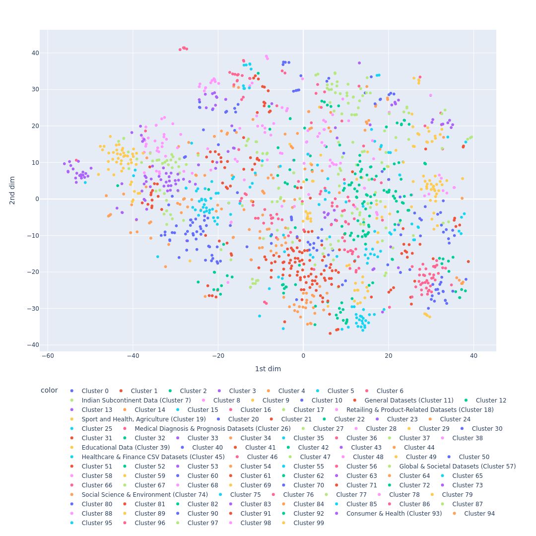
Figure 10: TSNE representation of total 100 domains clustered by K-Means algorithm, including manually labeled clusters.

We utilized the $k$-means algorithm to cluster BERT embeddings of table names, setting $K$ to 100. Figure 1 showcases the top 10 clusters containing the most elements. The clustering effectively categorized the data by table names, with each cluster representing specific domains such as consumer, health, and education data. However, as shown in Figure 10, distinguishing domains purely based on table names within 100 clusters presents a challenge that requires future work.

Table 5: Statistics about the datasets

Dataset	Raw tables	Cleaned tables train/val/test	Avg. # columns	Avg. # rows	License
Kaggle Random	43514	1148/143/144	8.37	224.8	Kaggle
Kaggle Domains	43514	969/218/248	8.37	224.8	Kaggle
GitTables	1M	1006/126/126	9.51	1112.68	CC BY 4.0

G.1.2 GitTables Dataset

GitTables Hulsebos et al. [2023] is a large-scale corpus of relational tables extracted from CSV files on GitHub, designed to facilitate the development of table representation models and applications in areas such as data management and data analysis. The corpus includes 1 million raw tables. Despite their tabular format, the majority of tables in the GitTables dataset contain unstructured data such as text (e.g., product reviews) or time series (e.g. server bandwidth). This presents a challenge in building foundational models for tabular data, requiring a significant effort in data cleaning. After removing tables with sole structured information there are 1258 tables split into train/val/test as illustrated in Table 5.

G.2 Data Cleaning

We recognize that the tabular datasets from both Kaggle and GitTables are quite noisy. Although they are in a structured format, most of the tables include a mix of structured information such as text, temporal and spatial data, along with irrelevant values like ID columns, missing values, and formatting errors. Below, we summarize the main steps of data cleaning. Some of these steps are automated, while a few require manual inspection and curation.

Files merging and cleaning After downloading the tables, we discovered variations in their structures. For examples, some datasets comprise CSV files serving as annotation labels for tasks like computer vision or natural language processing, such as image classification, with two columns: image path and label, or question answering in NLP, with two columns: text and IOB-label. Conversely, other datasets consisted of multiple tables, necessitating manual merging to create a comprehensive final table. This manual processing demands a profound understanding of the data and its associated task. To ensure suitability for pre-training the TabularFM task, we conducted a data cleaning and validation pipeline:

• Single Tabular File: We check if the downloaded dataset contains only one tabular file of CSV type. If the dataset fails this criterion, it is masked for manually merging.

• Manually merge: In cases the dataset fails the Single Tabular File criterion, we check that which data has a clear description about the dataset (have clear metadata about columns name, discription, columns type,) in Kaggle platform. We manually merged the columns and saved the final table to a single CSV file.

• Automated Validation of Annotation CSV Tables: As mentioned above, datasets containing CSV file annotation labels for computer vision or NLP downstream tasks are unsuitable for pre-training TabularFM. However, these datasets consistently have discernible patterns, typically characterized by all columns only contains two types of column: categories (text type labels), or texts (long string, paths, URLs). Leveraging this consistency, we implement automated validation procedures to effectively filter datasets having these characteristics.

Data Filtering Based on Column Types To optimize the quality of the acquired datasets, we apply a filtering step based on the column types. We remove columns containing non-numeric and non-categorical data types, including long string types, path strings, links, URLs, phone numbers, etc.

Noisy column identification, missing value imputation To ensure the effective training, we further construct automated preprocessing across datasets. For each column in a dataset, we automatically process the data based on the following criteria

• Remove identity data: since identity has no meaning in generation process, we discard columns with identity values such as id columns.

• Timestamp columns: any data representing date or timestamp is also removed. Since timestamp data is specialized for time-series generative models, which is out of scope for this work.

• Remove sparse categorical columns: we calculate frequency of each category. We discard the column if the number of categories is significantly large, i.e. greater than 90%, compared to the total number of samples. Furthermore, if the average frequency across categories is less than a threshold, we also discard the column. For the two proposed datasets, we set this threshold as 3%.

• Data imputation: empty cells in tables are imputed with conventional strategy. Particularly, if the total number of null values exceed a threshold, which is set to 50% in this work, the column will be discarded. Otherwise, we impute the data depends on the data type. For numerical column, average data is calculated, for categorical column, we impute the value of highest mode category.

Afterwards, a dataset may lose large number of columns. We then further discard a table if there are few columns left compared to a threshold. We eliminate tables which number of unqualified columns exceeds 90% in this work.

Appendix H Training Details

Let $\boldsymbol{\mathcal{D}}=\{\mathcal{D}_{i}\}$ be the whole datasets across domains. We divided them into three kinds of datasets as $\boldsymbol{\mathcal{D}}^{\text{pretrain}}$, $\boldsymbol{\mathcal{D}}^{\text{val}}$, $\boldsymbol{\mathcal{D}}^{\text{test}}$ correpsonding to pretraining datasets, validation and test datasets, respectively. Our objective is to study the transferability of tabular datasets. To this end, we train a model on $\boldsymbol{\mathcal{D}}^{\text{pretrain}}$ to achieve a pretrained model, the model is then finetuned on each dataset of $\boldsymbol{\mathcal{D}}^{\text{val}}$ and $\boldsymbol{\mathcal{D}}^{\text{test}}$. Along with that, we initialize a corresponding model for each dataset and train from scratch, i.e. single training. We then evaluate and compare the performance of fine-tuning versus training from scratch.

H.1 Pretraining

Let $\boldsymbol{\mathcal{M}}^{p}$ be the model training on $\boldsymbol{\mathcal{D}}^{\text{pretrain}}$. To avoid catastrophic forgetting , for each iteration, we train the model across dataset $\boldsymbol{\mathcal{D}}^{\text{pretrain}}$ with a single epoch and repeat for the next iteration. We randomly shuffle $\boldsymbol{\mathcal{D}}^{\text{pretrain}}$ for every iteration. The pretraining procedure can be describe in detail as follow

1. Initialize $\boldsymbol{\mathcal{M}}^{p}$

2. For each iteration

   1. Randomly shuffle $\boldsymbol{\mathcal{D}}^{\text{pretrain}}$

   2. For each dataset $\mathcal{D}_{i}\in\boldsymbol{\mathcal{D}}^{\text{pretrain}}$, transform and fit data to $\boldsymbol{\mathcal{M}}^{p}$ with epoch = 1

H.2 Fine-tuning and Single Training

For each dataset $\mathcal{D}_{i}\in\boldsymbol{\mathcal{D}}^{\text{val / test}}$, we initialize $\boldsymbol{\mathcal{M}}_{i}^{\text{ft}}$ with weights from $\boldsymbol{\mathcal{M}}^{p}$ and finetune the model. Our framework employs early stopping on loss of validation set of each dataset to prevent overfitting. For GAN-based models, since it is challenging to early stop the training only observing the validation loss, we keep checkpoints during the training.For single training, we initialize a model $\boldsymbol{\mathcal{M}}_{i}^{\text{st}}$ and train from scratch for each $\mathcal{D}_{i}\in\boldsymbol{\mathcal{D}}^{\text{val / test}}$. We also leverage early stopping in the training except for GAN-based models.

In summary, for each dataset $\mathcal{D}_{i}\in\boldsymbol{\mathcal{D}}^{\text{val / test}}$, the training procedure of finetuning is described as follow

1. Initialize $\boldsymbol{\mathcal{M}}_{i}^{\text{ft}}$ weights from $\boldsymbol{\mathcal{M}}^{p}$

2. For each epoch

   1. Transform and fit data of $\mathcal{D}_{i}$ to $\boldsymbol{\mathcal{M}}^{\text{ft}}$

   2. Early stopping checking

   3. Checkpoint checking

For each dataset $\mathcal{D}_{i}\in\boldsymbol{\mathcal{D}}^{\text{val / test}}$, the training procedure of single training is

1. Initialize $\boldsymbol{\mathcal{M}}_{i}^{\text{st}}$ from scratch

2. For each epoch

   1. Transform and fit data of $\mathcal{D}_{i}$ to $\boldsymbol{\mathcal{M}}^{\text{st}}$

   2. Early stopping checking

   3. Checkpoint checking

H.3 Evaluation

To evaluate the performance of tabular generation, we compare the quality of synthetic data versus real data by two properties. We measure the distribution of columns data between synthetic and real data, called Column Shapes. Correlation among columns is also computed, then compare the difference between ones of synthetic and real data, called Column Trends. We then average the two metrics as Overall Score. Formally, given a dataset $\mathcal{D}=\{D_{0},D_{1},\dots,D_{N_{d}},C_{0},C_{1},\dots,C_{N_{c}}\}$, the overall evaluation score, and score of column shape, trend are calculated as

$$\mathcal{S}^{(\mathcal{D})}=\frac{\mathcal{S}_{\text{shape}}^{(\mathcal{D})}+\mathcal{S}_{\text{trend}}^{(\mathcal{D})}}{2}$$ (19)

$$\mathcal{S}_{\text{shape}}^{(\mathcal{D})}=\frac{1}{N_{c}+N_{d}}\sum_{c\in N_{c},N_{d}}\mathcal{S}_{\text{shape}}^{(c)}$$ (20)

$$\mathcal{S}_{\text{trend}}^{(\mathcal{D})}=\frac{1}{N_{c}+N_{d}}\sum_{c\in N_{c},N_{d}}\mathcal{S}_{\text{trend}}^{(c)}$$ (21)

We describe the definition of scores to calculate on the table columns as follows. To avoid complication, we omit the annotation of dataset and columns, syn and real are added to represent the synthetic data and real data. In practice, the following metrics are computed separately for finetuned model and trained from scratch model. We then evaluate the performance between model finetuned from a pretraining, and model trained from scratch by comparing between those measurements.

H.3.1 Column Shapes

For numerical data, we leverage a non-parametric statistical method, which is Kolmogorov-Smirnov test Massey Jr [1951], to represent the fitness of shapes between distribution of synthetic and real data. Formally, let $F_{\text{syn}}(x)$ and $F_{\text{real}}(x)$, $x\in C_{i}$, denote the Cumulative Distribution Functions over distribution data of numerical columns of synthetic and real data, respectively. The score $\mathcal{S}_{\text{shape}}\in[0,1]$ represents the similarity between distribution of numerical synthetic and real data is described as follow (higher is better)

$$\mathcal{S}_{\text{shape}}=1-\sup_{x}|F_{\text{syn}}(x)-F_{\text{real}}(x)|$$ (22)

For categorical data, Total Variance Distance is computed to measure the column shapes. To this end, let $\Omega$ be the space of categories of $D_{i}$, we calculate the ratio of each category $w\in\Omega$, then measure the difference between ones of synthetic and real data. As a result, the score of column shape is adjusted to express higher is better as follow

$$\mathcal{S}_{\text{shape}}=1-\frac{1}{2}\sum_{w\in\Omega}|R_{\text{syn}}(w)-R_{\text{real}}(w)|$$ (23)

H.3.2 Column Trends

To measure the closeness of column pair trends between real and synthetic data, we measure every column pairs first and calculate the average. To this end, correlation is computed among columns in real and synthetic data separately, and then measure the difference. Depend on the data types, different methods are applied.

To measure the correlation between two numerical column, we leverage Pearson correlation Freedman et al. [2007]. Let $\rho(C_{m},C_{n})$ denote the Pearson correlation between two numerical columns $C_{m},C_{n}\in D$,

$$\rho(C_{m},C_{n})=\frac{\mathbb{E}\left((C_{m}-\mu_{C_{n}})(C_{n}-\mu_{C_{n}})\right)}{\sigma_{C_{m}}\sigma_{C_{n}}}$$ (24)

where $\mu_{*}$ and $\sigma_{*}$ represents the mean and standard deviation of column. As a result, $\rho_{\text{syn}}(C_{m},C_{n})$ and $\rho_{\text{real}}(C_{m},C_{n})$ is obtained, the column trend score between two numerical columns is defined as

$$\mathcal{S}_{\text{trend}}=1-\frac{|\rho_{\text{syn}}(C_{m},C_{n})-\rho_{\text{real}}(C_{m},C_{n})|}{2}$$ (25)

In the case of two categorical columns, we calculate a normalized contingency table. In other words, we compute the number of samples of any category pairs $w_{m},w_{n}\in\Omega$, then normalize by total number of samples, each combination is represented by $R(w_{m},w_{n})$. After that, Total Variance Distance is applied to calculate the column trend score. Given $D_{m},D_{n}\in D$ as pair of categorical columns. The correlation (higer is better) is express as

$$\mathcal{S}_{\text{trend}}=1-\frac{1}{2}\sum_{w_{m}\in\Omega_{D_{m}}}\sum_{w_{n}\in\Omega_{D_{n}}}|R_{\text{syn}}(w_{m},w_{n})-R_{\text{real}}(w_{m},w_{n})|$$ (26)

When dealing with column pairs of categorical and numerical data types, we first transform numerical to categorical data by grouping it into bins, and calculate the column trend score by (26).

References

- He et al. [2016] Kaiming He, Xiangyu Zhang, Shaoqing Ren, and Jian Sun. Deep residual learning for image recognition. In Proceedings of the IEEE conference on computer vision and pattern recognition, pages 770–778, 2016.
- Waswani et al. [2017] A Waswani, N Shazeer, N Parmar, J Uszkoreit, L Jones, A Gomez, L Kaiser, and I Polosukhin. Attention is all you need. In NIPS, 2017.
- Lin et al. [2023] Zeming Lin, Halil Akin, Roshan Rao, Brian Hie, Zhongkai Zhu, Wenting Lu, Nikita Smetanin, Robert Verkuil, Ori Kabeli, Yaniv Shmueli, et al. Evolutionary-scale prediction of atomic-level protein structure with a language model. Science, 379(6637):1123–1130, 2023.
- Ross et al. [2022] Jerret Ross, Brian Belgodere, Vijil Chenthamarakshan, Inkit Padhi, Youssef Mroueh, and Payel Das. Large-scale chemical language representations capture molecular structure and properties. Nature Machine Intelligence, 4(12):1256–1264, 2022. doi:10.1038/s42256-022-00580-7.
- LeCun et al. [2015] Yann LeCun, Yoshua Bengio, and Geoffrey Hinton. Deep learning. nature, 521(7553):436–444, 2015.
- van Breugel and van der Schaar [2024] Boris van Breugel and Mihaela van der Schaar. Why tabular foundation models should be a research priority. In International Conference on Machine Learning, 2024.
- Hulsebos et al. [2023] Madelon Hulsebos, Çagatay Demiralp, and Paul Groth. Gittables: A large-scale corpus of relational tables. Proceedings of the ACM on Management of Data, 1(1):1–17, 2023.
- Xu et al. [2019] Lei Xu, Maria Skoularidou, Alfredo Cuesta-Infante, and Kalyan Veeramachaneni. Modeling tabular data using conditional gan. Advances in neural information processing systems, 32, 2019.
- Lin et al. [2018] Zinan Lin, Ashish Khetan, Giulia Fanti, and Sewoong Oh. Pacgan: The power of two samples in generative adversarial networks. In S. Bengio, H. Wallach, H. Larochelle, K. Grauman, N. Cesa-Bianchi, and R. Garnett, editors, Advances in Neural Information Processing Systems, volume 31. Curran Associates, Inc., 2018. URL https://proceedings.neurips.cc/paper_files/paper/2018/file/288cc0ff022877bd3df94bc9360b9c5d-Paper.pdf.
- Gulrajani et al. [2017] Ishaan Gulrajani, Faruk Ahmed, Martin Arjovsky, Vincent Dumoulin, and Aaron C Courville. Improved training of wasserstein gans. In I. Guyon, U. Von Luxburg, S. Bengio, H. Wallach, R. Fergus, S. Vishwanathan, and R. Garnett, editors, Advances in Neural Information Processing Systems, volume 30. Curran Associates, Inc., 2017.
- Jelinek [1980] Frederick Jelinek. Interpolated estimation of markov source parameters from sparse data. 1980. URL https://api.semanticscholar.org/CorpusID:61012010.
- Bengio et al. [2000] Yoshua Bengio, Réjean Ducharme, and Pascal Vincent. A neural probabilistic language model. In T. Leen, T. Dietterich, and V. Tresp, editors, Advances in Neural Information Processing Systems, volume 13. MIT Press, 2000.
- Borisov et al. [2023] Vadim Borisov, Kathrin Sessler, Tobias Leemann, Martin Pawelczyk, and Gjergji Kasneci. Language models are realistic tabular data generators. In The Eleventh International Conference on Learning Representations, 2023.
- Radford et al. [2018] Alec Radford, Karthik Narasimhan, Tim Salimans, Ilya Sutskever, et al. Improving language understanding by generative pre-training. 2018.
- Radford et al. [2019] Alec Radford, Jeffrey Wu, Rewon Child, David Luan, Dario Amodei, Ilya Sutskever, et al. Language models are unsupervised multitask learners. OpenAI blog, 1(8):9, 2019.
- Brown et al. [2020] Tom Brown, Benjamin Mann, Nick Ryder, Melanie Subbiah, Jared D Kaplan, Prafulla Dhariwal, Arvind Neelakantan, Pranav Shyam, Girish Sastry, Amanda Askell, et al. Language models are few-shot learners. Advances in neural information processing systems, 33:1877–1901, 2020.
- Xu and Veeramachaneni [2018] Lei Xu and Kalyan Veeramachaneni. Synthesizing tabular data using generative adversarial networks. arXiv preprint arXiv:1811.11264, 2018.
- Joffe [2021] Leonid Joffe. Transfer learning for tabular data. November 2021. doi:10.36227/techrxiv.16974124.v1. URL http://dx.doi.org/10.36227/techrxiv.16974124.v1.
- Iida et al. [2021] Hiroshi Iida, Dung Thai, Varun Manjunatha, and Mohit Iyyer. TABBIE: Pretrained representations of tabular data. In Proceedings of the 2021 Conference of the North American Chapter of the Association for Computational Linguistics: Human Language Technologies, page 3446—3456, Online, 2021. Association for Computational Linguistics. doi:10.18653/v1/2021.naacl-main.270.
- Deng et al. [2021] Xiang Deng, Huan Sun, Alyssa Whitlock Lees, Will Wu, and Cong Yu. Turl: Table understanding through representation learning. In Proceedings of the VLDB Endowment, 2021.
- Yang et al. [2024] Yazheng Yang, Yuqi Wang, Guang Liu, Ledell Wu, and Qi Liu. Unitabe: A universal pretraining protocol for tabular foundation model in data science. In International Conference on Learning Representations, 2024.
- Arik and Pfister [2021] Sercan O Arik and Tomas Pfister. Tabnet: Attentive interpretable tabular learning. In Proceedings of the AAAI Conference on Artificial Intelligence, 2021.
- Nam et al. [2023] Jaehyun Nam, Jihoon Tack, Kyungmin Lee, Hankook Lee, and Jinwoo Shin. Stunt: Few-shot tabular learning with self-generated tasks from unlabeled tables. arXiv preprint arXiv:2303.00918, 2023.
- Hollmann et al. [2022] Noah Hollmann, Samuel Müller, Katharina Eggensperger, and Frank Hutter. Tabpfn: A transformer that solves small tabular classification problems in a second. arXiv preprint arXiv:2207.01848, 2022.
- Wang and Sun [2022] Zifeng Wang and Jimeng Sun. Transtab: Learning transferable tabular transformers across tables. Advances in Neural Information Processing Systems, 35:2902–2915, 2022.
- Padhi et al. [2021] Inkit Padhi, Yair Schiff, Igor Melnyk, Mattia Rigotti, Youssef Mroueh, Pierre Dognin, Jerret Ross, Ravi Nair, and Erik Altman. Tabular transformers for modeling multivariate time series. In ICASSP 2021-2021 IEEE International Conference on Acoustics, Speech and Signal Processing (ICASSP), pages 3565–3569. IEEE, 2021.
- Zhang et al. [2023] Han Zhang, Xumeng Wen, Shun Zheng, Wei Xu, and Jiang Bian. Towards foundation models for learning on tabular data, 2023.
- Hegselmann et al. [2023] Stefan Hegselmann, Alejandro Buendia, Hunter Lang, Monica Agrawal, Xiaoyi Jiang, and David Sontag. Tabllm: Few-shot classification of tabular data with large language models. In International Conference on Artificial Intelligence and Statistics, pages 5549–5581. PMLR, 2023.
- Dinh et al. [2022] Tuan Dinh, Yuchen Zeng, Ruisu Zhang, Ziqian Lin, Michael Gira, Shashank Rajput, Jy yong Sohn, Dimitris Papailiopoulos, and Kangwook Lee. Lift: Language-interfaced fine-tuning for non-language machine learning tasks. In Conference on Neural Information Processing Systems, 2022.
- Blei and Jordan [2006] David M Blei and Michael I Jordan. Variational inference for dirichlet process mixtures. 2006.
- Sennrich et al. [2016] Rico Sennrich, Barry Haddow, and Alexandra Birch. Neural machine translation of rare words with subword units. In Katrin Erk and Noah A. Smith, editors, Proceedings of the 54th Annual Meeting of the Association for Computational Linguistics (Volume 1: Long Papers), pages 1715–1725, Berlin, Germany, August 2016. Association for Computational Linguistics. doi:10.18653/v1/P16-1162. URL https://aclanthology.org/P16-1162.
- Massey Jr [1951] Frank J Massey Jr. The kolmogorov-smirnov test for goodness of fit. Journal of the American statistical Association, 46(253):68–78, 1951.
- Freedman et al. [2007] David Freedman, Robert Pisani, and Roger Purves. Statistics (international student edition). Pisani, R. Purves, 4th edn. WW Norton & Company, New York, 2007.
TabularFM: an Open Framework for Tabular Foundational Models
Supplementary Material