AAffil[arabic] \DeclareNewFootnoteANote[fnsymbol]
HiP Attention: Sparse Sub-Quadratic Attention with Hierarchical Attention Pruning
Abstract
In modern large language models (LLMs), increasing sequence lengths is a crucial challenge for enhancing their comprehension and coherence in handling complex tasks such as multi-modal question answering. However, handling long context sequences with LLMs is prohibitively costly due to the conventional attention mechanism’s quadratic time and space complexity, and the context window size is limited by the GPU memory. Although recent works have proposed linear and sparse attention mechanisms to address this issue, their real-world applicability is often limited by the need to re-train pre-trained models. In response, we propose a novel approach, Hierarchically Pruned Attention (HiP), which simultaneously reduces the training and inference time complexity from to and the space complexity from to . To this end, we devise a dynamic sparse attention mechanism that generates an attention mask through a novel tree-search-like algorithm for a given query on the fly. HiP is training-free as it only utilizes the pre-trained attention scores to spot the positions of the top- most significant elements for each query. Moreover, it ensures that no token is overlooked, unlike the sliding window-based sub-quadratic attention methods, such as StreamingLLM. Extensive experiments on diverse real-world benchmarks demonstrate that HiP significantly reduces prompt (i.e., prefill) and decoding latency and memory usage while maintaining high generation performance with little or no degradation. As HiP allows pretrained LLMs to scale to millions of tokens on commodity GPUs with no additional engineering due to its easy plug-and-play deployment, we believe that our work will have a large practical impact, opening up the possibility to many long-context LLM applications previously infeasible.
1 Introduction
Large transformer-based generative models trained on huge datasets have recently demonstrated remarkable abilities in various problem domains, such as natural language understanding (NLU) [38], code generation [34], and multi-modal question answering [25]. This is made possible by the effectiveness of the self-attention mechanism, which is the core of the Transformer architecture that learns pairwise relationships between all tokens in the given sequence of tokens. Despite their success, as the model size and cost of state-of-the-art Transformer-based generative models continue to grow, the quadratic complexity of the attention mechanism is increasingly becoming a critical obstacle, which is exacerbated with a growing demand to deal with with longer sequences.
To overcome this limitation, previous works have suggested different approaches to more efficiently handle longer sequences. FlashAttention [9, 8] has reduced the inference space complexity to by fusing the attention score and context computation to avoid storing attention scores. However, its time complexity still remains , which could be a critical limitation when running inference with long contexts (10k+tokens). Many other works [20, 4, 41, 35, 16, 36, 28] tackle the issue by sparsifying the attention matrix, either statically or dynamically, or approximate attention mechanism using kernel methods in order to reduce the time and space complexity of the attention mechanism. However, these works are not widely employed in real-world LLM services because they often lead to performance degeneration due to drastic changes in the computation flow and/or are too complex to implement efficiently to achieve actual speedups. Moreover, they often require a large amount of fine-tuning or even pre-training from scratch, which can be prohibitively expensive and prevent the timely deployment of the production-ready pre-trained models.
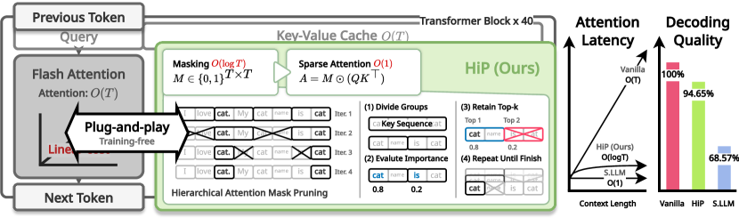
To address this problem, we propose Hierarchical Pruned Attention (HiP), a modified attention method which scales sub-quadratically (almost linearly) with the sequence length , as shown in Fig. 1. HiP consists of two parts: (1) mask estimation and (2) sparse attention computation, neither of which requires training (LABEL:fig:concept). HiP dynamically generates a sparse attention mask on the fly that restricts the number of accessible tokens from each query into while still allowing access to every key-values, unlike what is done in previous works [39, 40, 4]. This is done by dividing the input key-value sequence into groups, and then further dividing them into half, evaluating the importance of the tokens in each group while retaining the top important groups globally, until the groups cannot be further divided. This mask estimation process utilizes the pretrained attention scores for importance evaluation and does not require additional training. Since the masking process requires iterations and performs mask estimation for each query, the complexity of masking iterations is . Moreover, the generated sparse mask reduces the attention computation to complexity, which dominates the wall-clock decoding throughput in practice, since we cache the generated mask for successive queries during a few token decoding steps. In sum, HiP makes it feasible to quickly process extremely long sequences of tokens without incurring large training and inference costs, complex engineering, or performance degradation.
Furthermore, HiP considers modern hardware characteristics from the bottom of the method design. In contrast to previous approaches [20, 16], our method is aware of the tensor processing unit (e.g., TensorCore) by processing each masking and sparse attention process in tiled computation pattern [37]. Since we divide the sequence into sub-groups and perform hierarchical pruning, our method naturally considers memory locality with tiled memory accessing. Also, our method is easily integrated into throughput-optimized LLM serving frameworks, such as vLLM [19].
We validate HiP by applying it on Llama2 [38] and Qwen1.5 [2] models and compare its language modeling performance onWikiText2 [30], NLU performance on MMLU [14], and long context NLU performance on LongBench [3] and BookSum [17]. Our empirical findings show that HiP can speed up attention decoding by up to 36.92 times compared to FlashAttention2 [8] and speed up end-to-end model decoding 3.30 times compared to PagedAttention [18], widely used in the most LLM serving frameworks [19, 24, 7]. This dramatic practical speedup is achieved without any performance loss. The average performance obtained using HiP was % () on MMLU and % () on Booksum ROUGE-1 without any further training or healing, and % () on MMLU and % () on BookSum ROUGE-1 with only 1k steps of fine-tuning. In long context benchmark [3], our method significantly outperforms the baseline, StremaingLLM [39], by with Qwen1.5-14B. Our method obtains good performance with the large multimodal models (LMMs) [27] achieving () relative scores on a subset of LMMS-eval [22]. We also provide the kernel implementation with OpenAI Triton [37] and LLM serving framework using HiP attention based on vLLM [19].
We believe that this increased context length within the same computational budget opens up a new world of a wide variety of long-context applications, including question answering and inference with long textbooks, multi-agent chatbots with access to all of its previous chat history, enhanced retrieval-augmented reasoning, and summarization of long video data, to name just a few. Furthermore, our method design is hardware-friendly due to awareness of tensor processing units and is production-ready by implementing HiP Paged attention. Therefore, we expect our work to have a large practical impact on long-context LLM applications.
2 Related Works
Efficient Attention.
In prior works, several attention approximation methods with linear complexity were proposed, using kernel methods or sparse attention mechanisms. By low-rank approximation of softmax attention using kernel method, Performer [6] and Cosformer [32] could achieve extremely fast inference speed with linear complexity. However, since the low-rank approximation changes the inference data flow graph by a large amount, the performance degradation of the kernel-based approaches is not negligible and hard to recover from. In contrast to low-rank approximation, sparse attention methods use attention pruning. The sparse attention methods can maintain trained attention scores; they recover well after a simple replacement (plug-and-play) of the pre-trained attention mechanisms [20, 28]. Still, sparse attention requires further fine-tuning in order to adapt to the new static attention patterns [4, 40], or train the attention estimator [20, 28]. Furthermore, most implementations of them [16, 39, 20] are not as efficient as fused attention [9, 8], because they cannot utilize tensor processing unit due to their fine-grained sparsities. A tensor processing unit (block matrix multiplication unit) is a critical feature of modern accelerators that computes a part of matrix multiplication in one or a few cycles instead of computing every fused-multiply-add one by one.
StreamingLLM [39].
StreamingLLM uses a sliding window attention with an attention sink, which processes the input sequence in linear complexity without resetting the KV cache; they call this process ‘streaming.’ StreamingLLM introduces the attention sink, which is similar to the global attention token in Longformer [4], and streams the KV cache using RoPE indexing. However, due to the sliding window, the method cannot perform long-context knowledge retrieval. Therefore, this method cannot utilize the full context, and they do not extend the context window of the model by any amount. Since the method loses the key-value memory as time passes, it cannot take advantage of the transformer’s strength: its powerful past knowledge retrieval ability. Furthermore, since they use a different RoPE indexing for every query-key dot-product, they cannot utilize a tensor processing unit, which is a critical speedup factor in modern accelerators.
HyperAttention [13].
HyperAttention introduces sortLSH, improved version of LSH [16], to work as plug-and-play. The method uses block sparsity to utilize tensor processing units. It is training-free, has sub-quadratic time complexity (near-linear), and has the ability to potentially access to every past key token, much like our method. However, HyperAttention struggles to recover vanilla performance when replacing most of the layers in the trained model in a training-free manner (see Tab. 1).
Sparse Linear Attention with Estimated Attention Mask (SEA) [20].
Inspired by SEA’s framework, which introduces linear complexity attention estimation and sparse matrix interpolation, we aimed to improve its efficiency. SEA estimates each query’s attention probabilities over the keys with a fixed-size vector, turns it into a sparse mask by selecting the top-k elements, and resizes it; this process is done with linear complexity. However, the method is difficult to implement efficiently due to its extra modules, mainly the estimator and sparse matrix interpolation. Furthermore, the method does not support block sparsity; thus, it cannot utilize the tensor processing unit. We were motivated to improve this work drastically by introducing a fused and train-free attention mask estimator, HiP.
3 Methodology
Given query, key, and value sequences , the single-head attention output is computed as , , , where denotes embedding dimension and softmax is applied row-wise. The and matrices are respectively called the attention scores and probabilities. The conventional attention mechanism computes all of the pairwise relationships between the elements of the query and key sequences of length , which results in the time and space complexity of . However, is this really necessary? Our intuition tells us that humans do not, and cannot pay attention to all of the tokens in a document at any one time. Therefore, we hypothesize that in each attention head, for each query, we only need to attend to a fixed number of key tokens that have the largest attention score values without loss of performance. Based on this assumption, we approximate the attention mechanism with the following sparse linear attention mechanism:
| (1) | |||
| (2) | |||
| (3) |
where denotes the binary selecting the top- largest elements for each row of the given matrix. Since is a sparse matrix with only valid elements, and in Eq. 2 can be computed in time using sparse matrix operations. However, it is less straightforward to obtain the binary mask in sub-quadratic time. In Sec. 3.1, we show our novel method of obtaining a good approximation of in sub-quadratic time. Our method can easily be extended to causal self-attention, which is the form of attention that is most widely used in recent state-of-the-art LLMs.
3.1 Hierarchical Sparse Attention Mask Estimation
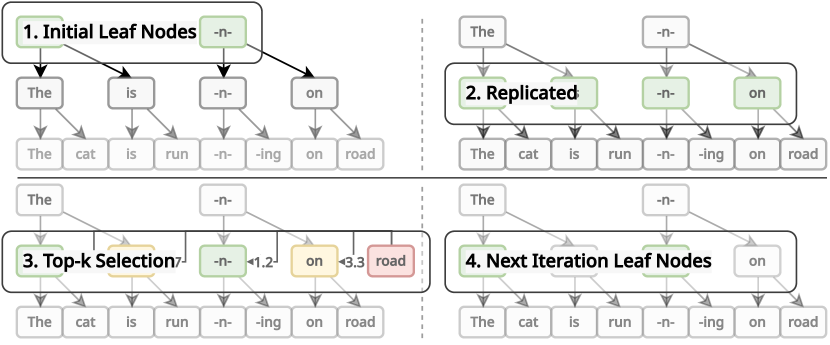
As shown in Eq. 1, our goal of estimating the attention mask is to select the top- largest elements of each pre-trained attention score row. However, we cannot compute all attention scores for each query because that would require time. Therefore, we need an efficient mask estimation method that can approximately select the top attention scores in sub-quadratic time. To this end, we use a greedy binary tree search algorithm, as illustrated in Fig. 2.
For a given query , we perform: In the first iteration, we divide the key sequence along the time dimension into equal-sized ranges (which we call nodes) , where and are the first and last indices of the th node, respectively.[1][1][1] denotes rounding to the nearest integer. The superscripts denote the iteration.
At each iteration , given the nodes, we further divide each node into two equal-sized branches:
A representative key index is the first key token index in the node for each branch . We assume that this representative key represents the entire branch. Thus, among the branches, the top branches whose representative key’s scores are the highest are chosen for the next iteration:
| (4) |
We repeat the above iteration times, in other words, until the length of each node’s range becomes 1. In the end, we obtain a set of indices , which is our estimation of the top- indices of which have the largest attention scores with the query . In other words, we obtain an estimation of a row of the attention mask [2][2][2], where is a set, denotes the indicator function: if , and otherwise .:
| (5) |
In conclusion, this algorithm takes time in total because the total number of iterations is where each iteration takes constant time , and we do this for each of the queries.
3.1.1 Block Approximation
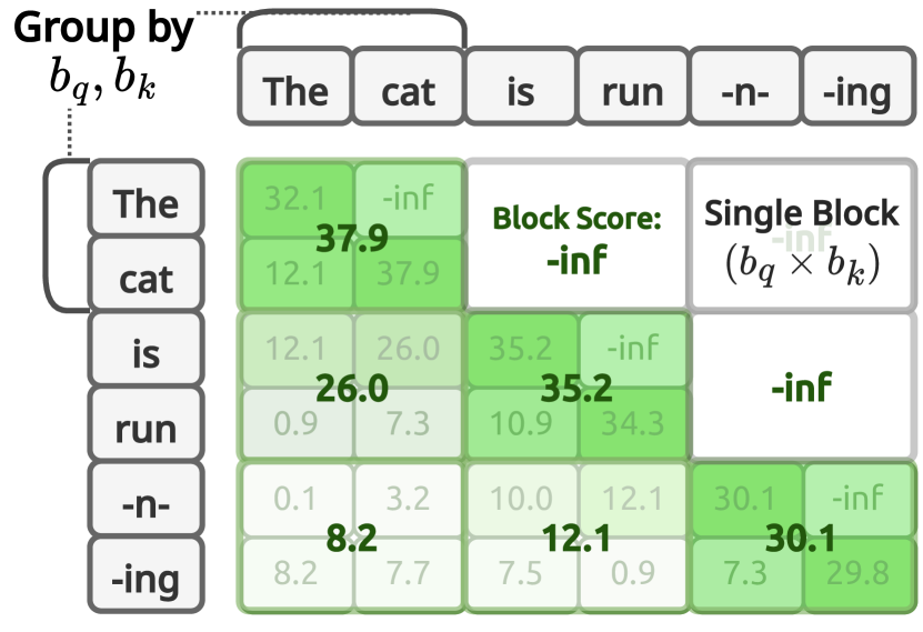
Despite the log-linear complexity, obtaining competitive wall-clock latency to the state-of-the-art implementations of quadratic dense attention on the conventional accelerator (e.g., GPU) is difficult in practice. This is because dense attention can fully utilize the accelerators’s tensor processing units (e.g., NVIDIA TensorCore, AMD MatrixCore, Google TPU, and Intel AMX), which are optimized to compute a fixed-size blocks of matrix multiplication in one or few clock cycles. In contrast, in HiP, the attention score computation in the mask estimation step cannot be performed with traditional matrix multiplication because a different key matrix is used to compute the dot product for each query vector. To enable tensor processing units and speed up the mask estimation, we use a technique called block approximation, illustrated in Fig. 3.
For the purpose of mask estimation, we replace with its reshaped version , and with its reshaped version , where and are the size of a key block and a query block. The mask estimation iterations are done similarly to before, except that the division and branching of the key sequence are done block-wise (using the first dimension of the tensor), and the score calculation in Eq. 4 is replaced with where is the given query block. In other words, we compare the maximum score values in the representative -sized block of each branch.
As a result of this optimization, the estimated mask contains repeated rows and columns. Therefore, each -block of the query can be matrix-multiplied with the same key matrix to obtain elements of . Thus, is a critical metric to determine the utilization of the tensor processing unit. We can achieve a considerable latency reduction if we set to a multiple of 16 or 32, as shown in Sec. D.4. While the choice of is irrelevant to the batch computation of matrix multiplication in inference time, it helps reduce the number of masking iterations performed in .
3.1.2 HiP on Large Multimodal Models
The large multimodal models (LMMs) process inputs beyond language tokens from domains such as image [26, 27], video [42], and audio [29] modalities, and therefore the burden on the self-attention mechanism grows and need to handle longer context in general. Our HiP can seamlessly substitute the self-attention in these LMMs as well, ensuring that the efficiency gains observed in LLMs can be also extended to LMMs.
The complete algorithm for mask estimation is presented in Alg. 1 in the appendix.
4 Experiments
4.1 Experiment Settings
In this section, we briefly introduce our overall experiment settings. We use StreamingLLM [39] as our main baseline because it has characteristics similar to our method: (1) sub-quadratic time complexity, (2) plug-and-play, and (3) availability of an efficient GPU implementation. Also, for the same reason, we choose the HyperAttention [13] as one of our baselines.
We replace the last attention layer with HiP in the pretrained LLM, where stands for the number of total layers and stands for the dense attention layer that remains in the patched model. Although our method uses few layers of dense attention due to the performance trade-off, we minimized the number of dense layers by performing an ablation study (Sec. D.5) and also introduced a novel ensemble method (App. E) that enables HiP to be stand-alone without requiring any dense layers. Furthermore, during LLM decoding, we cache the sparse attention mask from the previous decoding step and refresh it for every steps to minimize latency.
4.2 Performance Evaluation
Large Language Models (LLMs) are one of the most prominent models that utilize the attention mechanism. Thus, we first apply our proposed HiP to LLaMA2 [38] and Qwen1.5 [2], a collection of pretrained LLMs that are reported to perform well on various natural language understanding (NLU) tasks, to evaluate the effectiveness of our HiP mechanism.
| LLaMA2-7B | LLaMA2-13B | |||||||
| Method | Latency (s, 4k, dec) | Latency (s, 32k, dec) | Latency (ms, 32k, prm) | PPL ,(4k) | Latency (s, 4k, dec) | Latency (s, 32k, dec) | Latency (ms, 32k, prm) | PPL (4k) |
| Vanilla PyTorch | 72.17 (1.00) | 576.31 (1.00) | OOM | 5.5933 | 90.17 (1.00) | 719.72 (1.00) | OOM | 4.9613 |
| FlashAttention | 70.70 (1.02) | 562.76 (1.02) | 56.64 (1.00) | 5.5933 (+0.00) | 88.45 (1.02) | 705.34 (1.02) | 71.17 (1.00) | 4.9613 (+0.00) |
| HyperAttention (=3) pp | - | - | 81.51 (0.70) | 11.2828 (+5.69) | - | - | 101.60 (0.70) | 14.3881 (+9.43) |
| HyperAttention (=6) pp | - | - | 81.51 (0.70) | 9.1542 (+3.56) | - | - | 101.60 (0.70) | 12.0476 (+7.09) |
| StreamingLLM (k=512) pp | 14.87 (4.85) | 15.36 (37.52) | - | 6.2444 (+0.65) | 18.25 (4.94) | 18.79 (38.30) | - | 5.7928 (+0.83) |
| StreamingLLM (k=1024) pp | 28.94 (2.49) | 29.61 (19.46) | - | 5.8437 (+0.25) | 35.76 (2.52) | 36.33 (19.81) | - | 5.2842 (+0.32) |
| HiP (k=512) pp | 13.83 (5.22) | 15.62 (36.90) | 18.80 (3.01) | 5.7938 (+0.20) | 17.39 (5.19) | 19.67 (36.58) | 23.40 (3.04) | 5.1150 (+0.15) |
| HiP (k=1024) pp | 23.74 (3.04) | 26.94 (21.39) | 29.33 (1.93) | 5.6726 (+0.08) | 29.70 (3.04) | 33.97 (21.19) | 36.46 (1.95) | 5.0149 (+0.05) |
| HiP (k=512) heal | 13.83 (5.22) | 15.62 (36.90) | 18.80 (3.01) | 5.6872 (+0.09) | 17.39 (5.19) | 19.67 (36.58) | 23.40 (3.04) | 5.2902 (+0.32) |
4.2.1 Language Modeling Performance Evaluation (WikiText2)
We use the commonly used WikiText2 dataset [30] to evaluate the performance of HiP. We replace the top attention layers of the model with HiP except for the bottom layers while keeping every pretrained weight and evaluating the perplexity score. We also fine-tune the pretrained models using QLoRA [10] on the OpenWebText2 corpus [12] and perform the same evaluation. Additionally, we measure the latency in the two stages of text generation: (1) The initial pass (prompt phase), where the forward pass is computed on the entire prompt, and (2) the subsequent passes (decoding phase), which are performed with cached key-value pairs and the query is only one token long each time.
In Tab. 1, our proposed HiP attention is faster in prompt latency and faster in decoding latency in LLaMA2-13B while only suffering increase in perplexity, which is reduced to only with further finetuning. Since our method fully utilizes the tensor processing unit by block approximation, we could achieve a similar latency with the sliding window method, StreamingLLM [39]. While the sliding window-based method StreamingLLM could recover performance well with only a point degradation, the other sub-quadratic attention method HyperAttention [13] show a worse performance drop than StreamingLLM and ours, losing points. We describe further detail about the HyperAttention experiment setting in App. C.
4.2.2 Massive Multitask Language Understanding (MMLU)
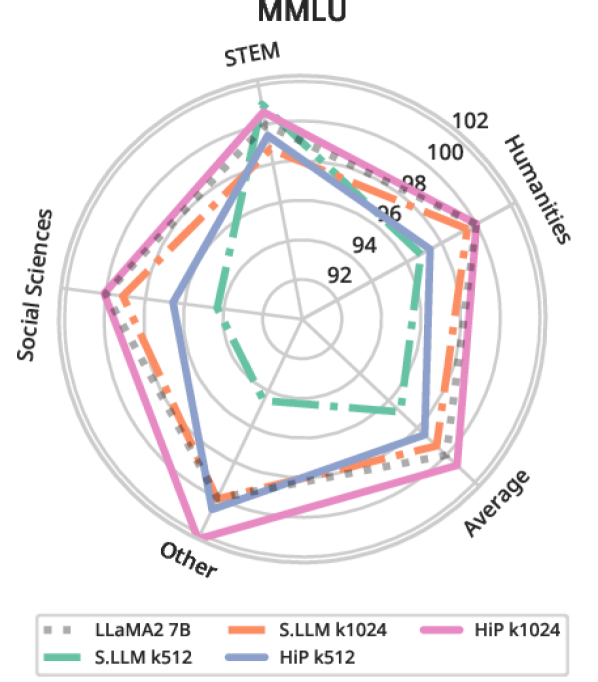
Next, we evaluate HiP on the MMLU benchmark [14] to show that our method does not negatively affect the NLU ability of the pretrained model. We report the average scores for each field of study and the total average scores in Fig. 4, with the details shown in Tab. 6. The results show that our HiP preserves the NLU performance of the original model. Specifically, HiP achieves 43.08% (+0.32%p) accuracy with plug-and-play, and 43.79% (+1.03%p) accuracy with healing in MMLU on the LLaMA2-7B. StreamingLLM [39] shows slightly worse performance at 42.47% (-0.29%p), compared to ours. Surprisingly, StreamingLLM’s performance degradation is not very significant here. This is probably due to the nature of the MMLU task: the answer is only dependent on the most recent span of tokens rather than the entire prompt (which contains few-shot examples in the beginning).

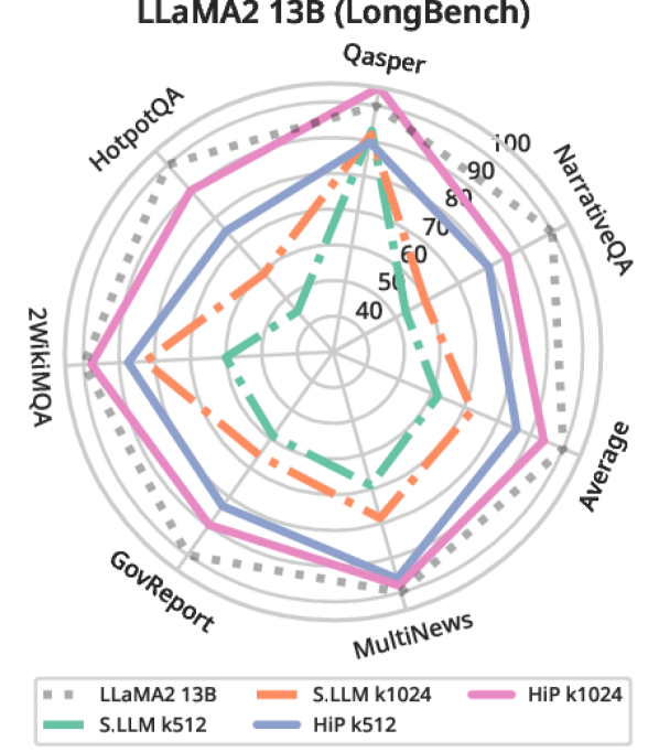
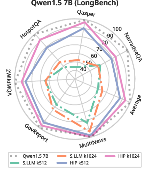
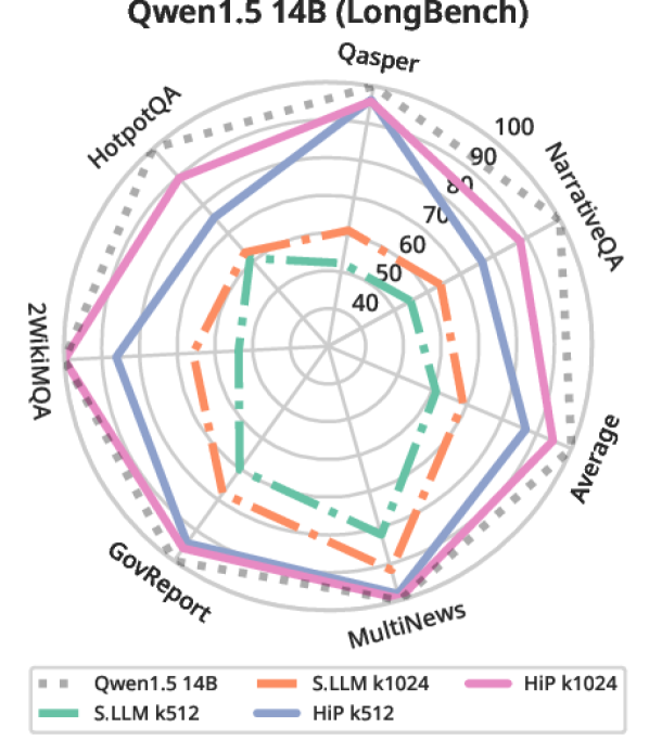
4.2.3 Long Context Natural Language Understanding Benchmark (LongBench)
We then use the LongBench benchmark [3] to evaluate the long context prompt and decoding performance of HiP in Fig. 5, with the details shown in Tab. 7. We select a subset of LongBench by following StreamingLLM’ssetting [39]. We believe that this benchmark is the most important because it shows both long context generation performance and knowledge retrieval performance, which are critical in many LLM applications, such as multi-turn assistants and in-context learning. Our method significantly outperforms the baseline because, unlike StreamingLLM, HiP has the potential to access every available previous token. StreamingLLM tends to fail to retrieve long context information because it uses a sliding window, which forces the model to look at local information. We illustrate this long context knowledge retrieval ability by using an example from LongBench in Sec. D.1.
| LLaMA2-7B | LLaMA2-13B | |||||
| Method | ROUGE-1 | ROUGE-2 | ROUGE-L | ROUGE-1 | ROUGE-2 | ROUGE-L |
| Vanilla zs | 25.28% | 4.05% | 15.72% | 31.45% | 6.03% | 16.94% |
| StreamingLLM (k=512) zs | 21.20% | 2.82% | 12.83% | 25.29% | 3.95% | 14.19% |
| StreamingLLM (k=1024) zs | 22.33% | 2.95% | 13.68% | 26.80% | 4.51% | 15.00% |
| HiP (Ours) (k=512) zs | 23.01% | 3.10% | 14.31% | 28.45% | 5.05% | 15.66% |
| HiP (Ours) (k=1024) zs | 24.95% | 3.74% | 15.27% | 29.96% | 5.65% | 16.32% |
| Vanilla bs | 37.82% | 9.03% | 18.88% | 32.75% | 7.32% | 16.94% |
| HiP (Ours) (k=512) bs | 34.88% | 8.03% | 17.69% | 31.48% | 6.77% | 16.42% |
| HiP (Ours) (k=512) bs + heal | 38.21% | 9.23% | 18.97% | 32.67% | 7.17% | 16.73% |
4.2.4 Long Document Summarising (BookSum)
We use the BookSum benchmark [17] to evaluate the long-context long-response generation quality of HiP. We report the average ROUGE F1 scores [23] of the generated summaries in Tab. 2. We show that our method can preserve dense attention’s performance in BookSum, with only a 0.33%p drop in ROUGE-1 score on LLaMA2-7B. Here, we try to fine-tune the HiP-applied transformer for the downstream task. We describe the detailed training procedure in Sec. A.6.
4.2.5 Large Multimodal Model with HiP

Since large multi-modal models (LMM) [26, 27] leverage pre-trained LLMs as a backbone for their NLU ability, without changes, except for the tokenizer, we also evaluated our HiP on top of LLaVA-1.6-13B [27], a large multi-modal model, using LMMs-eval [22], which provides extensive benchmarks for large multimodal model suites. As we show in Fig. 6 and Tab. 9, our method scores 98.87% relative scores, which is similar to the performance recovery ratio of HiP on NLU tasks. Surprisingly, StreamingLLM fails on this task, while it achieves competitive performance recovery in NLU tasks. Our method outperforms StreamingLLM in every multimodal dataset, and ours sometimes even scores 3.75 higher.
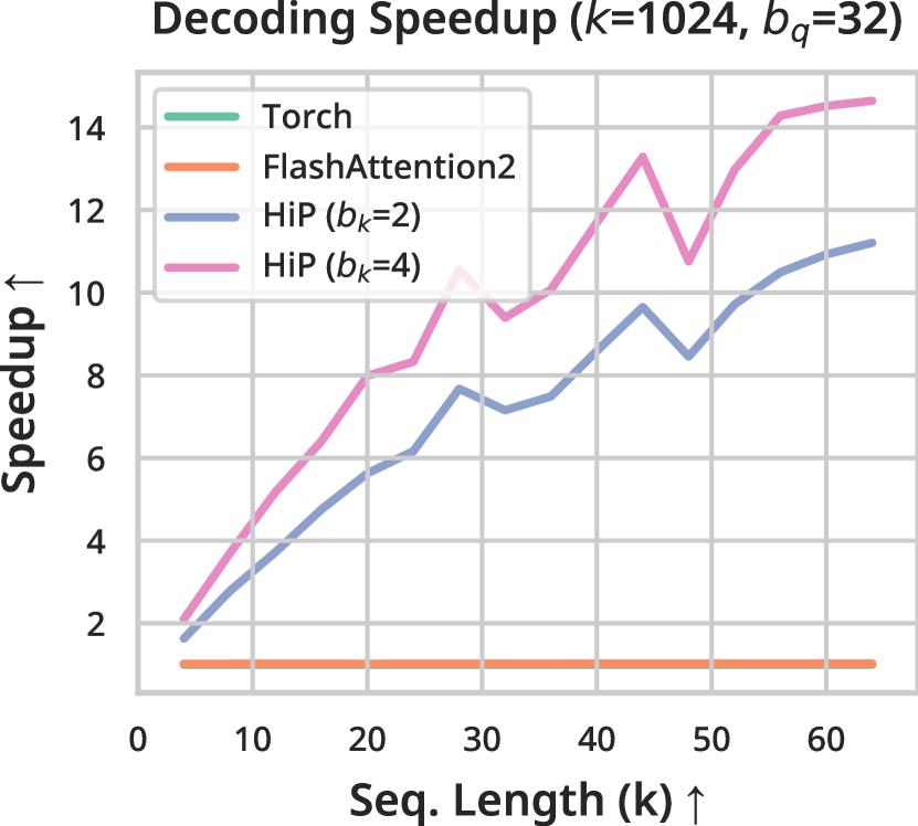


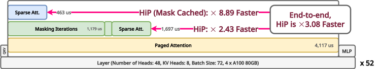
4.3 Latency Micro-benchmark and Breakdown
We evaluate the trade-off between attention latency and the model performance with HiP in Fig. 7. In Fig. 7, we show that the latency optimized setting shows about 5.5 speedup of attention decoding latency and achieves 4.83 (+0.15) perplexity in Wikitext2. In Fig. 8, we show the latency breakdown of the HiP-applied transformer model. Our proposed method contains two major components that contribute to the overall latency: (1) masking iterations and (2) sparse flash attention. Since the masking iteration results could be cached and reused times (Sec. 4.4), the latency of the HiP method is dominated by sparse flash attention in most practical scenarios. Therefore, for users, is the most important efficiency factor of HiP.
| Context length (B.S.) | 8,192 (82) | 16,384 (41) | 32,768 (23) | 65,536 (11) | ||||
| Metric | Latency | Lat. / B.S. | Latency | Lat. / B.S. | Latency | Lat. / B.S. | Latency | Lat. / B.S. |
| vLLM | 67.14 | 0.82 (1.00) | 68.72 | 1.68 (1.00) | 60.14 | 2.61 (1.00) | 55.62 | 5.06 (1.00) |
| HiP (Ours) (k=512) | 47.70 | 0.58 (1.41) | 40.72 | 0.99 (1.69) | 34.30 | 1.49 (1.75) | 28.61 | 2.60 (1.94) |
| HiP (Ours) (k=1024) | 68.33 | 0.83 (0.98) | 49.91 | 1.22 (1.38) | 45.64 | 1.98 (1.32) | 34.53 | 3.14 (1.61) |
4.4 vLLM End-to-end Decoding Latency Benchmark
We evaluate the end-to-end token generation latency of the HiP attention method on a widely used LLM serving framework, vLLM [19], in Tab. 3. The latency speedup in this section is the actual end-to-end model decoding speedup that users will observe in a real-world scenario. We measure only the model decoding latency and exclude the preparation and token sampling latencies of vLLM because these parts are orthogonal to our work, do not dominate the latency, and can be pipelined with the model decoding part. We implement the HiP GPU kernel with PagedAttention proposed in [19]. In Tab. 3, we observe up to 1.94 speedup with our method compared to the baseline (PagedAttention [19]). However, the speedup does not increase linearly with the context length due to the limitation in parallelism in our GPU implementation, which we describe in more detail in Sec. 5. With a larger batch size, we achieve a 3.30 improvement in total serving throughput as shown in Tab. 4. Also, we perform an ablation study about mask refreshing interval in Sec. D.6.
5 Limitations
| Luxia-21B (GQA) | Qwen1.5-14B (MHA) | ||||||
| 1 | 16 | 64 | 1 | 8 | 16 | ||
| 16k | vLLM | 13.48 (1.00) | 39.19 (1.00) | 122.09 (1.00) | 7.175 (1.00) | 17.72 (1.00) | 29.32 (1.00) |
| HiP (Ours) | 15.77 (0.85) | 31.45 (1.25) | 54.29 (2.25) | 8.88 (0.81) | 18.46 (0.96) | 25.38 (1.16) | |
| 32k | vLLM | 15.24 (1.00) | 60.33 (1.00) | 205.50 (1.00) | 8.13 (1.00) | 24.78 (1.00) | 43.31 (1.00) |
| HiP (Ours) | 15.78 (0.97) | 32.63 (1.85) | 62.30 (3.30) | 8.88 (0.92) | 18.95 (1.31) | 26.56 (1.63) | |
Our masking kernel runs the jobs in parallel across the batch dimension and query dimensions, structured as where represents the batch size, denotes the head size, and denotes the query token count. We cannot divide the single parallel job into smaller ones because top- requires synchronization. Without speculative decoding, the kernel runs jobs; for instance, with a head size of 40, only 40 jobs are active with a batch size of 1. Therefore, the number of jobs might be smaller than that of workers in hardware (e.g., streaming multiprocessors in NVIDIA).
We can tackle this issue in various ways: (1) increasing batch size, (2) partial top- masking, and (3) using speculative decoding. We can increase the batch size by using grouped query attention (GQA) [1] as shown in Tab. 4. This limitation also means that if we can increase the batch size enough, we can achieve much better throughput. Therefore, we show that speedup is drastically improved by increasing batch size in Tab. 4. Furthermore, we introduce stridden partial top- masking that splits the key-value sequence into chunks, allowing for simultaneous executions. Lastly, using speculative decoding, we can increase the dimension to increase the parallelism.
6 Conclusion
In this study, we have presented HiP Attention, a novel technique for accelerating pretrained Transformer-based models without any training. Our proposed HiP rapidly estimates the dynamic sparse mask for computing sparse attention, drastically reducing the computation time required for long context inference and fine-tuning from to . Our HiP attention is a drop-in replacement for the core of any Transformer-based models, such as language (LLM) and multimodal (LMM) models, and does not require changing the existing weights. This is a practical and meaningful improvement as it allows pre-trained models to be fine-tuned and executed much more efficiently in long sequences without sacrificing quality.
In the future, we are looking forward to contributing to the open-source LLM serving framework by combining various efficient decoding strategies with HiP attention. We expect a synergy effect with speculative decoding, KV cache eviction, and compression strategy since they are orthogonal with our method; please see Sec. D.7 and Sec. D.8 for further details. In further research, we will improve the overall accuracy of the mask estimation using ensembles (App. E) and a branch prediction of hierarchical pruning by learning optimal group splits and selection during hierarchical pruning. We further plan to overcome the memory limitation of the KV cache using an offloading policy where our method has a huge advantage, as shown in Sec. D.3.
Acknowledgment
This work was supported by Institute of Information & communications Technology Planning & Evaluation (IITP) grant funded by the Korea government (MSIT) (No. RS-2022-00187238, Development of Large Korean Language Model Technology for Efficient Pre-training).
References
- Ainslie et al. [2023] Ainslie, J., Lee-Thorp, J., de Jong, M., Zemlyanskiy, Y., Lebrón, F., and Sanghai, S. Gqa: Training generalized multi-query transformer models from multi-head checkpoints. arXiv preprint arXiv:2305.13245, 2023.
- Bai et al. [2024] Bai, J., Bai, S., Chu, Y., Cui, Z., Dang, K., Deng, X., Fan, Y., Ge, W., Huang, F., Hui, B., Li, M., Lin, J., Lin, R., Liu, D., Liu, T., Lu, K., Ma, J., Men, R., Ni, N., Ren, X., Ren, X., San, Z., Tan, S., Tu, J., Wang, P., Wang, S., Xu, J., Yang, A., Yang, J., Yang, K., Yang, S., Yao, Y., Yu, B., Zhang, J., Zhang, Y., Zhang, Z., Zheng, B., Zhou, C., Zhou, J., Zhou, X., and Zhu, T. Introducing Qwen1.5, 2024. URL http://qwenlm.github.io/blog/qwen1.5/. Section: blog.
- Bai et al. [2023] Bai, Y., Lv, X., Zhang, J., Lyu, H., Tang, J., Huang, Z., Du, Z., Liu, X., Zeng, A., Hou, L., Dong, Y., Tang, J., and Li, J. Longbench: A bilingual, multitask benchmark for long context understanding. arXiv preprint arXiv:2308.14508, 2023.
- Beltagy et al. [2020] Beltagy, I., Peters, M. E., and Cohan, A. Longformer: The long-document transformer, 2020. URL http://arxiv.org/abs/2004.05150.
- Cai et al. [2024] Cai, T., Li, Y., Geng, Z., Peng, H., Lee, J. D., Chen, D., and Dao, T. Medusa: Simple llm inference acceleration framework with multiple decoding heads, 2024.
- Choromanski et al. [2022] Choromanski, K., Likhosherstov, V., Dohan, D., Song, X., Gane, A., Sarlos, T., Hawkins, P., Davis, J., Mohiuddin, A., Kaiser, L., Belanger, D., Colwell, L., and Weller, A. Rethinking attention with performers, 2022. URL http://arxiv.org/abs/2009.14794.
- Contributors [2024] Contributors, G. Tensorrt-llm, 2024. URL https://github.com/NVIDIA/TensorRT-LLM.
- Dao [2023] Dao, T. FlashAttention-2: Faster attention with better parallelism and work partitioning, 2023. URL http://arxiv.org/abs/2307.08691.
- Dao et al. [2022] Dao, T., Fu, D. Y., Ermon, S., Rudra, A., and Ré, C. FlashAttention: Fast and memory-efficient exact attention with IO-awareness, 2022. URL http://arxiv.org/abs/2205.14135.
- Dettmers et al. [2023] Dettmers, T., Pagnoni, A., Holtzman, A., and Zettlemoyer, L. QLoRA: Efficient finetuning of quantized LLMs, 2023. URL http://arxiv.org/abs/2305.14314.
- Fu et al. [2024] Fu, Y., Bailis, P., Stoica, I., and Zhang, H. Break the sequential dependency of llm inference using lookahead decoding. arXiv preprint arXiv:2402.02057, 2024.
- Gao et al. [2020] Gao, L., Biderman, S., Black, S., Golding, L., Hoppe, T., Foster, C., Phang, J., He, H., Thite, A., Nabeshima, N., Presser, S., and Leahy, C. The Pile: An 800gb dataset of diverse text for language modeling. arXiv preprint arXiv:2101.00027, 2020.
- Han et al. [2024] Han, I., Jayaram, R., Karbasi, A., Mirrokni, V., Woodruff, D., and Zandieh, A. Hyperattention: Long-context attention in near-linear time. In The Twelfth International Conference on Learning Representations, 2024. URL https://openreview.net/forum?id=Eh0Od2BJIM.
- Hendrycks et al. [2021] Hendrycks, D., Burns, C., Basart, S., Zou, A., Mazeika, M., Song, D., and Steinhardt, J. Measuring massive multitask language understanding, 2021. URL http://arxiv.org/abs/2009.03300.
- Inan et al. [2023] Inan, H., Upasani, K., Chi, J., Rungta, R., Iyer, K., Mao, Y., Tontchev, M., Hu, Q., Fuller, B., Testuggine, D., and Khabsa, M. Llama guard: Llm-based input-output safeguard for human-ai conversations, 2023.
- Kitaev et al. [2019] Kitaev, N., Kaiser, L., and Levskaya, A. Reformer: The efficient transformer. In ICLR 2020, 2019. URL https://openreview.net/forum?id=rkgNKkHtvB.
- Kryściński et al. [2022] Kryściński, W., Rajani, N., Agarwal, D., Xiong, C., and Radev, D. BookSum: A collection of datasets for long-form narrative summarization, 2022. URL http://arxiv.org/abs/2105.08209.
- Kwon et al. [2023a] Kwon, W., Li, Z., Zhuang, S., Sheng, Y., Zheng, L., Yu, C. H., Gonzalez, J. E., Zhang, H., and Stoica, I. Efficient memory management for large language model serving with pagedattention, 2023a.
- Kwon et al. [2023b] Kwon, W., Li, Z., Zhuang, S., Sheng, Y., Zheng, L., Yu, C. H., Gonzalez, J. E., Zhang, H., and Stoica, I. Efficient memory management for large language model serving with pagedattention. In Proceedings of the ACM SIGOPS 29th Symposium on Operating Systems Principles, 2023b.
- Lee et al. [2023] Lee, H., Kim, J., Willette, J., and Hwang, S. J. SEA: Sparse linear attention with estimated attention mask, 2023. URL http://arxiv.org/abs/2310.01777.
- Leviathan et al. [2023] Leviathan, Y., Kalman, M., and Matias, Y. Fast inference from transformers via speculative decoding. In International Conference on Machine Learning, pp. 19274–19286. PMLR, 2023.
- Li* et al. [2024] Li*, B., Zhang*, P., Zhang*, K., Pu*, F., Du, X., Dong, Y., Liu, H., Zhang, Y., Zhang, G., Li, C., and Liu, Z. Lmms-eval: Accelerating the development of large multimoal models, March 2024. URL https://github.com/EvolvingLMMs-Lab/lmms-eval.
- Lin [2004] Lin, C.-Y. ROUGE: A package for automatic evaluation of summaries. In Text Summarization Branches Out, pp. 74–81, Barcelona, Spain, July 2004. Association for Computational Linguistics. URL https://aclanthology.org/W04-1013.
- Lin* et al. [2024] Lin*, Y., Tang*, H., Yang*, S., Zhang, Z., Xiao, G., Gan, C., and Han, S. Qserve: W4a8kv4 quantization and system co-design for efficient llm serving. arXiv preprint arXiv:2405.04532, 2024.
- Liu et al. [2023a] Liu, H., Li, C., Li, Y., and Lee, Y. J. Improved baselines with visual instruction tuning, 2023a. URL http://arxiv.org/abs/2310.03744.
- Liu et al. [2023b] Liu, H., Li, C., Wu, Q., and Lee, Y. J. Visual instruction tuning. In NeurIPS, 2023b.
- Liu et al. [2024] Liu, H., Li, C., Li, Y., Li, B., Zhang, Y., Shen, S., and Lee, Y. J. Llava-next: Improved reasoning, ocr, and world knowledge, January 2024. URL https://llava-vl.github.io/blog/2024-01-30-llava-next/.
- Liu et al. [2021] Liu, L., Qu, Z., Chen, Z., Ding, Y., and Xie, Y. Transformer acceleration with dynamic sparse attention, 2021. URL http://arxiv.org/abs/2110.11299.
- Lyu et al. [2023] Lyu, C., Wu, M., Wang, L., Huang, X., Liu, B., Du, Z., Shi, S., and Tu, Z. Macaw-llm: Multi-modal language modeling with image, audio, video, and text integration. arXiv preprint arXiv:2306.09093, 2023.
- Merity et al. [2016] Merity, S., Xiong, C., Bradbury, J., and Socher, R. Pointer sentinel mixture models, 2016. URL http://arxiv.org/abs/1609.07843. version: 1.
- Miao et al. [2024] Miao, X., Oliaro, G., Zhang, Z., Cheng, X., Wang, Z., Zhang, Z., Wong, R. Y. Y., Zhu, A., Yang, L., Shi, X., Shi, C., Chen, Z., Arfeen, D., Abhyankar, R., and Jia, Z. Specinfer: Accelerating large language model serving with tree-based speculative inference and verification. In Proceedings of the 29th ACM International Conference on Architectural Support for Programming Languages and Operating Systems, Volume 3, ASPLOS ’24. ACM, April 2024. doi: 10.1145/3620666.3651335. URL http://dx.doi.org/10.1145/3620666.3651335.
- Qin et al. [2022] Qin, Z., Sun, W., Deng, H., Li, D., Wei, Y., Lv, B., Yan, J., Kong, L., and Zhong, Y. cosFormer: Rethinking softmax in attention, 2022. URL http://arxiv.org/abs/2202.08791.
- Ribar et al. [2013] Ribar, L., Chelombiev, I., Hudlass-Galley, L., Blake, C., Luschi, C., and Orr, D. SparQ attention: Bandwidth-efficient LLM inference, 2013. URL http://arxiv.org/abs/2312.04985.
- Rozière et al. [2024] Rozière, B., Gehring, J., Gloeckle, F., Sootla, S., Gat, I., Tan, X. E., Adi, Y., Liu, J., Sauvestre, R., Remez, T., Rapin, J., Kozhevnikov, A., Evtimov, I., Bitton, J., Bhatt, M., Ferrer, C. C., Grattafiori, A., Xiong, W., Défossez, A., Copet, J., Azhar, F., Touvron, H., Martin, L., Usunier, N., Scialom, T., and Synnaeve, G. Code llama: Open foundation models for code, 2024. URL http://arxiv.org/abs/2308.12950.
- Tay et al. [2020] Tay, Y., Bahri, D., Yang, L., Metzler, D., and Juan, D.-C. Sparse sinkhorn attention. In Proceedings of the 37th International Conference on Machine Learning, pp. 9438–9447. PMLR, 2020. URL https://proceedings.mlr.press/v119/tay20a.html. ISSN: 2640-3498.
- Tay et al. [2021] Tay, Y., Bahri, D., Metzler, D., Juan, D.-C., Zhao, Z., and Zheng, C. Synthesizer: Rethinking self-attention in transformer models, 2021. URL http://arxiv.org/abs/2005.00743.
- Tillet et al. [2019] Tillet, P., Kung, H.-T., and Cox, D. D. Triton: an intermediate language and compiler for tiled neural network computations. Proceedings of the 3rd ACM SIGPLAN International Workshop on Machine Learning and Programming Languages, 2019. URL https://api.semanticscholar.org/CorpusID:184488182.
- Touvron et al. [2023] Touvron, H., Martin, L., Stone, K., Albert, P., Almahairi, A., Babaei, Y., Bashlykov, N., Batra, S., Bhargava, P., Bhosale, S., Bikel, D., Blecher, L., Ferrer, C. C., Chen, M., Cucurull, G., Esiobu, D., Fernandes, J., Fu, J., Fu, W., Fuller, B., Gao, C., Goswami, V., Goyal, N., Hartshorn, A., Hosseini, S., Hou, R., Inan, H., Kardas, M., Kerkez, V., Khabsa, M., Kloumann, I., Korenev, A., Koura, P. S., Lachaux, M.-A., Lavril, T., Lee, J., Liskovich, D., Lu, Y., Mao, Y., Martinet, X., Mihaylov, T., Mishra, P., Molybog, I., Nie, Y., Poulton, A., Reizenstein, J., Rungta, R., Saladi, K., Schelten, A., Silva, R., Smith, E. M., Subramanian, R., Tan, X. E., Tang, B., Taylor, R., Williams, A., Kuan, J. X., Xu, P., Yan, Z., Zarov, I., Zhang, Y., Fan, A., Kambadur, M., Narang, S., Rodriguez, A., Stojnic, R., Edunov, S., and Scialom, T. Llama 2: Open foundation and fine-tuned chat models, 2023. URL http://arxiv.org/abs/2307.09288.
- Xiao et al. [2024] Xiao, G., Tian, Y., Chen, B., Han, S., and Lewis, M. Efficient streaming language models with attention sinks. In The Twelfth International Conference on Learning Representations, 2024. URL https://openreview.net/forum?id=NG7sS51zVF.
- Zaheer et al. [2020a] Zaheer, M., Guruganesh, G., Dubey, K. A., Ainslie, J., Alberti, C., Ontanon, S., Pham, P., Ravula, A., Wang, Q., Yang, L., and Ahmed, A. Big bird: Transformers for longer sequences. In Larochelle, H., Ranzato, M., Hadsell, R., Balcan, M., and Lin, H. (eds.), Advances in Neural Information Processing Systems, volume 33, pp. 17283–17297. Curran Associates, Inc., 2020a. URL https://proceedings.neurips.cc/paper_files/paper/2020/file/c8512d142a2d849725f31a9a7a361ab9-Paper.pdf.
- Zaheer et al. [2020b] Zaheer, M., Guruganesh, G., Dubey, K. A., Ainslie, J., Alberti, C., Ontanon, S., Pham, P., Ravula, A., Wang, Q., Yang, L., and Ahmed, A. Big bird: Transformers for longer sequences. In Advances in Neural Information Processing Systems, volume 33, pp. 17283–17297. Curran Associates, Inc., 2020b. URL https://proceedings.neurips.cc/paper/2020/hash/c8512d142a2d849725f31a9a7a361ab9-Abstract.html.
- Zhang et al. [2023a] Zhang, H., Li, X., and Bing, L. Video-llama: An instruction-tuned audio-visual language model for video understanding. arXiv preprint arXiv:2306.02858, 2023a. URL https://arxiv.org/abs/2306.02858.
- Zhang et al. [2023b] Zhang, Z., Sheng, Y., Zhou, T., Chen, T., Zheng, L., Cai, R., Song, Z., Tian, Y., Ré, C., Barrett, C., Wang, Z., and Chen, B. H2o: Heavy-hitter oracle for efficient generative inference of large language models, 2023b.
Appendix A Detailed Methodology Descriptions
A.1 Comparison of Time and Space Complexities
| Method | HiP (Ours) | SEA [20] | FlashAttention [8] | StreamingLLM [39] | HyperAttention (sortLSH) [13] | |
| Complexity | Time | Log-linear | Linear | Quadratic | Linear | Near-linear |
| Space | Linear | Linear | Linear | Linear | Near-linear | |
| Training Free (Plug-and-play) | ✓ | ✗ | ✓ | ✓ | ✓ | |
| Dynamic Attention | ✓ | ✓ | ✓ | ✗ | ✓ | |
| Method | Reformer (LSH) [16] | Performer [6] | Cosformer [32] | Longformer [4] | ||
| Complexity | Time | Log-linear | Linear | Linear | Linear | |
| Space | Log-linear | Linear | Linear | Linear | ||
| Training Free (Plug-and-play) | ✗ | ✗ | ✗ | ✗ | ||
| Dynamic Attention | ✓ | ✓ | ✓ | ✗ | ||
In Tab. 5, for each method, we show the time and space complexities, whether it is training-free, and whether it uses dynamic attention. Dynamic attention methods can attend to each other content dynamically rather than using static attention patterns such as a sliding window. Besides HiP, HyperAttention is the only method that satisfies all four criteria, but HyperAttention suffers from substantial performance degradation (see Tab. 1).
A.2 Hierarchical Sparse Attention Mask Estimation Algorithm
In Alg. 1, we describe the full algorithm used for mask estimation. The peak amount of memory used during the mask estimation process is in , since at each iteration, only the immediately previous iteration’s node indices are needed, and the rest can be discarded.
A.3 HiP Decoding Algorithm
In Alg. 2, we show a rough sketch of the decoding process with HiP. In particular, note the function of the mask estimation period and the number of initial dense layers , and the time and space complexities of each component.
A.4 Sparsity Inducing Attention Regularization
Since our approximation assumes that the attention probabilities are sparse, we employ an extra regularization term that encourages the attention probabilities to be sparse during the healing process. To this end, we aim to compute the norm with on the attention probability distributions for each layer. However, since this computation is quadratic and expensive, we instead sample query indices for each layer at each step and compute the norm for those indices only. We add the following regularization term to the loss only during the healing process:
| (6) |
where is the number of layers in the model, is the number of attention heads in the th layer, is the attention probability map at layer , head , and is a hyperparameter. indicates the th value of a random shuffling of the integers in the range . We set throughout the experiments.
A.5 Additional Optimization Techniques
A.5.1 Top-r Approximation
In order to reduce the cost of the mask estimator even further, we take inspiration from SparQ Attention [33], where global memory (HBM or GDDR) transfer is reduced by selectively fetching only the most relevant components of the key vectors. Specifically, when computing the inequality condition in Eq. 4, instead of fetching all components of the key vectors, we only fetch most prominent components estimated by the query vector . Thus, we compute the following as an approximation:
| (7) |
where . By using the top- approximation, the total number of global memory accesses in the mask estimation stage can be drastically reduced.
A.5.2 Block Sparse Flash Attention
We utilize the Flash Attention [9] mechanism to reduce the latency of sparse attention and use a small size sliding window to reduce performance degradation on the side of the sparse attention kernel. Following the receipt of StreamingLLM [39], local sliding window and global sink attention are also added during block sparse flash attention operation. The sliding window and sink attention are fixed sizes (128, 32) for every experiment in this paper.
A.6 Training Downstream Tasks with HiP
In this section, we describe the HiP attention training strategy for downstream tasks. We discovered that direct fine-tuning after applying HiP could not achieve the performance of the fine-tuned vanilla attention. Empirically, HiP’s highly sparse attention matrices show great performance approximation during test time but not in train gradients. Since our method heavily prunes the attention matrix, the gradient cannot flow through dense attention probabilities. This incomplete and unstable gradient of the attention matrix leads to significant training performance degradation because HiP forces the model to have attention patterns similar to those of the pretrained model rather than adopting them for the downstream task.
However, we could achieve the same performance as vanilla by using the following two-step training strategy: (1) fine-tuning with vanilla first and (2) further fintuning after applying HiP (healing). First, we train the pretrained model with vanilla attention to the downstream task as usual. Then, we load the finetuned weight, apply HiP, and further finetuning with the downstream task dataset with just a few optimizer steps. We call this a healing process because we only finetune a few steps from the finetuend weight. For training details about each experiment, we describe hyperparameter and optimization setups in App. C.
Appendix B Additional Experimental Results
B.1 Detailed Results on Massive Multitask Language Understanding (MMLU) with HiP and StreamingLLM
| LLaMA2-7B | LLaMA2-13B | |||||||||
| Method |
Humanities |
STEM |
Social Sciences |
Others | Average |
Humanities |
STEM |
Social Sciences |
Others | Average |
| Vanilla | 47.24 | 34.81 | 48.51 | 44.59 | 42.76 | 59.85 | 43.19 | 64.34 | 58.66 | 54.97 |
| StreamingLLM (k=512) pp | 45.74 | 35.17 | 45.76 | 42.16 | 41.40 (-1.36p) | 53.18 | 39.27 | 57.17 | 52.99 | 49.34 (-5.63p) |
| StreamingLLM (k=1024) pp | 47.00 | 34.37 | 48.09 | 44.61 | 42.47 (-0.29p) | 56.03 | 41.87 | 59.39 | 53.89 | 51.53 (-3.44p) |
| HiP (Ours) (k=512) pp | 45.99 | 34.61 | 46.85 | 44.87 | 42.12 (-0.64p) | 56.27 | 42.12 | 59.35 | 55.23 | 51.96 (-3.01p) |
| HiP (Ours) (k=1024) pp | 47.25 | 35.03 | 48.55 | 45.61 | 43.08 (+0.32p) | 57.27 | 42.00 | 59.68 | 55.85 | 52.37 (-2.60p) |
| HiP (Ours) (k=512) heal | 48.12 | 35.54 | 48.48 | 47.18 | 43.79 (+1.03p) | 58.62 | 44.10 | 62.87 | 56.85 | 54.27 (-0.70p) |
In Tab. 6, we evaluate our method and baselines on MMLU.
B.2 Detailed Results on LongBench with HiP and StreamingLLM
| Single Document QA | Multi Document QA | Summarization | |||||
| Method | NarrativeQA | Qasper | HotpotQA | 2WikiMQA | GovReport | MultiNews | Average |
| Context Length (k) | 35.96 22 | 5.64 3.0 | 15.27 4.5 | 8.42 4.1 | 13.11 8.1 | 3.44 2.6 | 13.64 |
| LLaMA2-7B | 4.35% | 12.37% | 14.70% | 12.33% | 30.75% | 27.21% | 16.95% |
| StreamingLLM (k=512) | 4.49% | 5.66% | 7.90% | 8.87% | 20.24% | 20.61% | 11.30% (-5.66%p) |
| StreamingLLM (k=1024) | 4.45% | 6.65% | 7.54% | 8.24% | 22.21% | 23.49% | 12.11% (-4.84%p) |
| HiP (Ours) (k=512) | 4.15% | 9.19% | 11.94% | 11.59% | 23.56% | 25.86% | 14.38% (-2.57%p) |
| HiP (Ours) (k=1024) | 3.38% | 11.05% | 11.79% | 12.15% | 26.88% | 26.05% | 15.22% (-1.74%p) |
| Qwen1.5-7B | 20.94% | 40.25% | 47.92% | 34.14% | 30.24% | 24.69% | 33.03% |
| StreamingLLM (k=512) | 13.37% | 17.79% | 23.46% | 22.09% | 20.18% | 20.49% | 19.56% (-13.47%p) |
| StreamingLLM (k=1024) | 12.82% | 21.18% | 27.07% | 21.93% | 22.29% | 23.08% | 21.40% (-11.64%p) |
| HiP (Ours) (k=512) | 16.50% | 36.29% | 37.89% | 29.88% | 27.92% | 24.25% | 28.79% (-4.24%p) |
| HiP (Ours) (k=1024) | 17.61% | 39.15% | 43.73% | 31.44% | 29.20% | 24.75% | 30.98% (-2.05%p) |
| LLaMA2-13B | 13.45% | 11.39% | 18.13% | 21.21% | 28.84% | 26.38% | 19.90% |
| StreamingLLM (k=512) | 7.16% | 10.58% | 8.18% | 12.76% | 17.00% | 18.16% | 12.31% (-7.59%p) |
| StreamingLLM (k=1024) | 8.00% | 10.46% | 10.74% | 17.54% | 18.92% | 20.68% | 14.39% (-5.51%p) |
| HiP (Ours) (k=512) | 10.72% | 10.21% | 13.64% | 18.56% | 23.99% | 25.33% | 17.08% (-2.83%p) |
| HiP (Ours) (k=1024) | 11.51% | 11.98% | 16.37% | 20.76% | 25.85% | 25.85% | 18.72% (-1.18%p) |
| Qwen1.5-14B | 22.85% | 39.83% | 53.82% | 41.35% | 29.84% | 24.41% | 35.35% |
| StreamingLLM (k=512) | 12.56% | 20.85% | 32.92% | 22.22% | 20.94% | 19.99% | 21.58% (-13.77%p) |
| StreamingLLM (k=1024) | 14.63% | 24.36% | 34.02% | 27.21% | 23.25% | 22.36% | 24.31% (-11.05%p) |
| HiP (Ours) (k=512) | 17.50% | 38.35% | 40.64% | 35.64% | 28.10% | 23.97% | 30.70% (-4.65%p) |
| HiP (Ours) (k=1024) | 20.12% | 38.19% | 48.17% | 41.35% | 28.61% | 24.29% | 33.46% (-1.90%p) |
B.3 Comparison with Reformer and SEA
We compare the performance of HiP against Reformer [16] and SEA [20] using the Llama2-7b model and show the results in Tab. 8. Even though HiP requires no fine-tuning, unlike Reformer and SEA, which need fine-tuning, our HiP attention is far superior in language modeling performance compared to these two baselines.
For a fair comparison, we fine-tune Reformer and SEA using LoRA (Low-rank adapters), which have the same rank as the healed version of HiP. Due to this, the Reformer and SEA’s performance converges to a much-degraded value compared to the values reported in their respective original papers. We conclude that both methods need much modification to the original weights in order to perform well, whereas since HiP performs well even without any modification to the weights whatsoever, a small amount of LoRA training can even close this small gap.
B.4 Detailed LMMs-Eval Results with LLaVA1.6
| Method | ChartQA | InfoVQA | MMMU | DocVQA | GQA | TextVQA | Relative Score |
| LLaVA-1.6-13B [27] | 62.20% | 41.34% | 35.90% | 77.38% | 65.36% | 66.92% | 100.00% |
| StreamingLLM [39] (k=512) | 16.40% | 29.90% | 31.30% | 24.75% | 51.71% | 26.76% | 56.17% (-43.83%p) |
| StreamingLLM [39] (k=1024) | 27.40% | 35.80% | 32.30% | 41.95% | 60.00% | 46.36% | 72.66% (-27.34%p) |
| HiP (Ours) (k=512, =2) | 56.60% | 39.56% | 35.30% | 69.21% | 64.65% | 62.51% | 94.46% (-5.54%p) |
| HiP (Ours) (k=512, =1) | 58.24% | 40.31% | 35.30% | 72.20% | 64.54% | 64.29% | 96.26% (-3.74%p) |
| HiP (Ours) (k=1024, =2) | 60.96% | 40.99% | 35.80% | 74.78% | 65.06% | 65.68% | 98.54% (-1.46%p) |
| HiP (Ours) (k=1024, =1) | 61.48% | 41.27% | 35.10% | 76.01% | 64.92% | 66.38% | 98.87% (-1.13%p) |
Appendix C Detailed Experimental Settings
Computation Resources. We use two machines to run experiments and training. (1) 4090 Machine. We use this local development machine. Most of the micro-benchmark and kernel optimization is done with this machine. (2x RTX 4090 24GB, 128GB DDR5-3600, Ryzen 7950x), (2) A100 Machine. We use this AWS cloud node as the main computation horse. All training and most long context benchmarks are measured with this machine. We use different GPU architectures for kernel development because we could not get an H100 AWS node due to a lack of quota. Therefore, our kernel’s CUDA hyper-parameters, such as the number of warps per program and block sizes, are not optimal in the A100 machine. To overcome these mismatches between the development machine and the computation horse, we used triton.autotune as much as possible. However, for the above reasons, the optimization of the GPU kernel may not be optimal for every GPU architecture.
Experiment Settings. By default, for the HiP experiment, we use . For StreamingLLM, we use .
We show overall experiment settings, such as the number of GPUs and model IDs to which the experiment is introduced (e.g., the caption of the figure and table). To reference, we leave the huggingface model path in Tab. 10. We used 4-bit quantization from huggingface transformers during generation.
| Model | Huggingface ID |
| LLaMA2-7b | togethercomputer/LLaMA-2-7B-32K |
| LLaMA2-13b | Yukang/Llama-2-13b-chat-longlora-32k-sft |
| Qwen1.5-7B | Qwen/Qwen1.5-7B-Chat |
| Qwen1.5-14B | Qwen/Qwen1.5-14B-Chat |
| Luxia-21.4B | saltlux/luxia-21.4b-alignment-v1.1 |
Experiment Details (Wikitext2). We provide the following experiment details for Tab. 1. The official implementation of HyperAttention is not available for decoding; therefore, we did not measure the decoding latency and decoding benchmark. We do not use HyperAttention in another experiment because it fails to recover the perplexity of wikitext2, the most basic metric of language modeling. Our implementation of StreamingLLM is not available for prompting due to a lack of support for block sparsity. Therefore, we do not measure the decoding latency. The decoding latency of StreamingLLM implementation without block sparsity is meaningless because it should be more than 32 times lower than block sparse one. However, since the method requires a different RoPE index for every query-key dot product, we cannot easily adopt block sparsity on their method. Measured with one NVIDIA RTX 4090. The batch size is 64 for the 4k decode, 32 for the 32k decode, and 1 for the 32k prompt sequence. For HyperAttention [13] we used lsh_num_projs=7, block_size=64, sample_size=1024, min_seq_len=32. We select min_seq_len to match the size of the tensor processing unit’s size () rather than , which is suggested by the authors’ code repository. Since in sortLSH [13] it processes shorter block size of min_seq_len with vanilla attention. Therefore, we have to reduce the size of its to a smaller size than , which is context length in perplexity measurement of Tab. 1.
Training Details (Healing HiP in Wikitext2). The HiP healing in Tab. 1 is done as follows. For the LLaMa2-7B model, after applying HiP, we fine-tune the pretrained model on the OpenWebText2 dataset for 1k steps with AdamW optimizer with learning rate 5e-5, and with batch size 16, LoRA rank 256, and HiP’s hyperparameters set to . For the LLaMa2-13B model, we use the same parameters as above, except it is trained for only 200 steps. The dataset is prepared as follows. We take the OpenWebText2 dataset hosted on huggingface and concatenate every thirty consecutive instances together into chunks. We then truncate each chunk to a max of 32k tokens.
Training Details (Finetuning BookSum with HiP). As for the training in Tab. 2, we first fine-tune the pretrained LLaMA2-7B and 13B models on the training split of the BookSum dataset for 1k and 250 steps with batch size 16 and 32, respectively, without using HiP. Then, after applying HiP, we further healed the model on the same dataset, both with batch size 32, for 100 and 150 steps (of which 20 and 100 are warm-up steps), respectively. For the latter stage, we use the learning rate 1e-5 for both models. Both stages of fine-tuning were done with LoRA rank 256 and with the same HiP hyperparameters as above. The BookSum dataset was downloaded from https://huggingface.co/datasets/togethercomputer/Long-Data-Collections from huggingface.
Appendix D Additional Analysis
D.1 Analysis of Summarizing Result between StreamingLLM and HiP
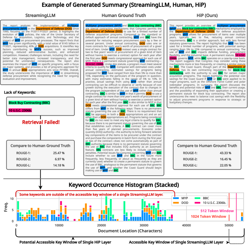
In Fig. 9, we analyze one example generation result from GovReport in LongBench. We pick four important keywords from the human ground truth summary: MYP, BBC, DOD, and 10 U.S.C 2306b. We pick two keywords (MYP, DOD) that appear in every summary and two keywords (BBC, 10 U.S.C 2306b) that appear only in the ground truth and HiP result. The result clearly shows that StreamingLLM is struggling to gather information beyond its single-layer window size, . StreamingLLM should be accessible to a much longer distance than because information keeps exchanging across time dimensions in each layer, like Mistral. In contrast to StreamingLLM, our proposed HiP attention shows successful knowledge retrieval in summary from long-range in-context documents, with the same plug-and-play manner. Also, quantitatively, ROUGE-* scores show that the summary generated by HiP is much better in coherence with ground truth than StreamingLLM.
D.2 Hierarchical Attention Mask Pruning Visualization
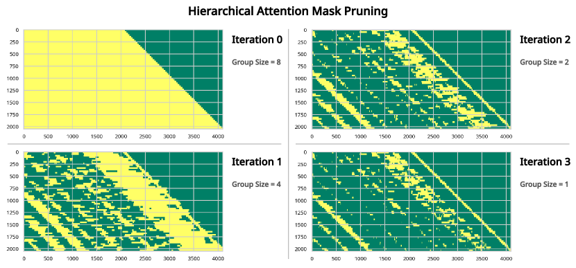
In Fig. 10, we demonstrate real-world examples of hierarchical attention mask pruning. We sample the Q, K, and V tensors from the first layer of LLaMA2-7B with a random text sample from Wikitext-2. Note that each attention mask in the masking iteration is not the final attention mask. The final attention mask generated by this process is from iteration 3. In an earlier iteration, the sparsity of the mask is low because the group size of blocks is very large (8), so the key values are treated as single groups. The attention score of that group is represented by the attention score between the query and the group’s first block ().
D.3 CUDA Unified Virtual Memory (UVM) Latency Evaluation
| Context Length | 16k | 32k | |||||||||||
| Metric | Prompt Lat. (s) | Dec. Lat. (ms) | Prompt Lat. (s) | Dec. Lat. (ms) | |||||||||
| No Offload | vLLM | 2 | 4.42 | 2.21 | 9 | 65.489 | 7.28 (1.00) | 1 | 4.60 | 4.60 | 5 | 54.883 | 10.98 (1.00) |
| HiP (Ours) | 2 | 4.44 | 2.22 | 9 | 41.742 | 4.64 (1.57) | 1 | 4.16 | 4.16 | 5 | 25.208 | 5.04 (2.18) | |
| V Offload | vLLM | 2 | 33.56 | 17.78 | 17 | 4,016.70 | 236.28 (1.00) | 1 | 31.46 | 31.46 | 9 | 3,778.34 | 419.82 (1.00) |
| HiP (Ours) | 2 | 5.63 | 2.82 | 17 | 365.04 | 21.47 (11.00) | 1 | 5.21 | 5.21 | 9 | 216.57 | 24.06 (17.45) | |
Since our method is a sparse attention method and the attention mask has temporal locality due to mask caching, our method accesses a fixed number and fixed location of the V cache during the attention mechanism. Also, our method accesses a fixed number and fixed location of the K cache during sparse attention. However, during masking iterations, our method accesses a fixed number of K cache per every iteration but not a fixed location. Therefore, we can expect we can offload the majority of the V cache from GPU VRAM, which is the main memory bottleneck of LLM decoding. However, since we have a low spatial locality of K cache access during the masking process, offloading the K cache may significantly increase latency. Therefore, in further research, we think the K cache must be compressed for mask estimation, and the raw K cache must be offloaded on the CPU during sparse attention. We adopt KV cache CPU offloading using CUDA unified virtual memory API for easier development. In Tab. 11, we show our method has an advantage on the K and V cache offloading scenarios.
D.4 Ablation Study of Block Size
| PPL. | 1 | 2 | 4 | 8 | 16 | 32 | Avg. | |
| 1 | 5.5210 | 5.5172 | 5.4996 | 5.4952 | 5.5064 | 5.5331 | 5.5121 | |
| 2 | 5.6032 | 5.6060 | 5.5863 | 5.5599 | 5.5577 | 5.5901 | 5.5839 | |
| 4 | 5.6316 | 5.6280 | 5.5971 | 5.5872 | 5.5838 | 5.5870 | 5.6024 | |
| 8 | 5.5807 | 5.5928 | 5.5553 | 5.5238 | 5.5100 | 5.5212 | 5.5473 | |
| Avg. | 5.5841 | 5.5860 | 5.5596 | 5.5415 | 5.5395 | 5.5578 | 5.5614 | |
| Lat. | 1 | 2 | 4 | 8 | 16 | 32 | Avg. | |
| 1 | 1.6416 | 1.6397 | 1.6397 | 1.6398 | 1.6397 | 1.6401 | 1.6401 | |
| 2 | 1.3543 | 1.3542 | 1.3530 | 1.3533 | 1.3535 | 1.3534 | 1.3536 | |
| 4 | 1.2312 | 1.2311 | 1.2296 | 1.2305 | 1.2322 | 1.2306 | 1.2309 | |
| 8 | 1.2836 | 1.2842 | 1.2830 | 1.2827 | 1.2830 | 1.2835 | 1.2833 | |
| Avg. | 1.3777 | 1.3773 | 1.3763 | 1.3766 | 1.3771 | 1.3769 | 1.3770 | |
| Lat. | 1 | 2 | 4 | 8 | 16 | 32 | Avg. | |
| 1 | 152.4423 | 77.2624 | 39.2077 | 20.1341 | 10.4925 | 5.5461 | 50.8475 | |
| 2 | 85.3140 | 43.8207 | 22.7708 | 12.1814 | 6.4987 | 3.5056 | 29.0152 | |
| 4 | 54.2530 | 27.7025 | 14.3960 | 7.9660 | 4.5839 | 2.6156 | 18.5862 | |
| 8 | 41.5079 | 21.3036 | 11.5369 | 7.4481 | 5.0634 | 3.0337 | 14.9823 | |
| Avg. | 83.3793 | 42.5223 | 21.9779 | 11.9324 | 6.6596 | 3.6753 | 28.3578 | |
We perform an ablation study on block sizes () using our method. Block size determines how many queries are grouped into the block during the masking iteration and sparse attention. And block size determines how many keys are grouped. Block size is a really important factor in utilizing tensor processing units (e.g., NVIDIA TensorCore) in modern accelerators. Tensor processing units enable matrix multiplication and tensor operations to be performed in single or fewer cycles rather than processing one by one using floating point multiplication and addition. This kind of trend of accelerator leads to mismatching of wall-clock latency and FLOPs in modern hardware. Therefore, we check the performance and latency trade-off among grouping queries and keys by block size .
In Tab. 12, we show that perplexity gets better as increases while it gets worse as increases. It is not intuitive that increasing shows better perplexity than before because they lose the resolution across the query dimension in attention mask estimation. However, the result shows that more block size (more averaging) across the query (time) dimension shows better performance. In contrast to this observation, works as expected, like that less resolution in key (past knowledge or memory) dimension leads to worse performance.
This phenomenon makes our method speed up without any performance loss, even achieving better performance. In Tab. 13, we measure the micro latency benchmark of our attention operation during the decoding stage, which feeds a single query into the attention operator. With a single query, we cannot utilize the tensor processing unit fully because, during sparse attention and attention score estimation in masking iteration, we cannot matrix multiply between the group and group. We have a single query vector; therefore, we need a vector-matrix multiplier instead of matrix-matrix multiplication, which is the main key feature or tensor processing unit. However, in Tab. 14, we measure the micro latency benchmark of our attention operation during the decoding stage with a speculative decoding strategy, which feeds multiple queries into the attention operator. We feed 32 query vectors within a query dimension in the input tensor; therefore, now we can utilize a matrix-matrix multiplier in a tensor processing unit. With these multiple queries and tensor processing unit utilization, our method could achieve 10.23 times speedup on 12k sequence length compared to PyTorch naive implementation (using bmm).
We use by default, according to the ablation study across the block sizes. We choose because increasing leads to better latency and perplexity. However, we stopped increasing by 32 because the current modern GPU, especially the NVIDIA Ampere series, usually does not support matrix-matrix multiplication larger than 32. And maybe in the future, some variants will support larger matrix multiplication, just like Google TPU. However, larger blocks need more register allocation for block masking and address calculation. Therefore, considering implementation limitations, we think there is no benefit to increasing infinitely. Also, from a performance perspective, we do not think this trend will keep over . We choose because latency speedup from to is huge respect to perplexity loss.
Additionally, we measure the latency with , which means without mask caching. Therefore, this speedup will be amplified with in a practical setting. As we show in Tab. 1, an attention speedup due to sub-quadratic complexity is more than 36 times.
D.5 Ablation Study of Dense Layers
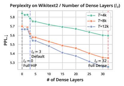
We do not replace the first few layers () of the Transformer because the first few layers tend to have dense attention probabilities rather than sparse attention probabilities. This phenomenon is well described in previous results [33]. The first few layers exchange information globally and uniformly across the tokens.
Therefore, in Fig. 11, we perform an ablation study on how many first layers should remain as dense attention. We observe that the first layers are kept as dense attention and then more perplexity. In other words, if we replace the original transformer block with HiP attention, we could minimize the performance degradation. However, for maximum practical speedup, we want to minimize the number of dense layers for the experiment. Therefore, we run the ablations study on different numbers of dense layers, and we choose 3. For 2 to 3, the performance (perplexity) improvement is maximized. In conclusion, the practical effect of dense layers on latency is minimal because the number of dense layers (e.g., 3, 4) is small compared to the number of HiP layers (e.g., 29, 36). We show that we could achieve practical end-to-end speedup compared to baselines in Tab. 3.
However, the more dense layer makes our end-to-end Transformer model complexity quadratic. To overcome this limitation, we also propose replacing dense layers with an ensemble of HiP attention masking in App. E.
D.6 Ablation Study of Mask Refreshing Interval in Decoding
| Method (Qwen 1.5-14B-GPTQ) | vLLM | HiP (=) | HiP (=) | HiP (=) | HiP (=) | HiP (=) | |
| k=512 | Latency (ms) | 68.72 | 38.95 (1.8) | 40.72 (1.7) | 44.01 (1.6) | 50.75 (1.4) | 63.62 (1.1) |
| ROUGE-1 | 32.46% | 29.53% | 29.95% | 30.19% | 30.38% | 30.47% | |
| ROUGE-2 | 6.28% | 5.13% | 5.40% | 5.54% | 5.55% | 5.49% | |
| ROUGE-L | 17.02% | 15.64% | 15.84% | 15.94% | 15.92% | 16.04% | |
| k=1024 | Latency (ms) | 68.72 | 45.11 (1.5) | 49.91 (1.4) | 53.06 (1.3) | 63.55 (1.1) | 81.69 (0.8) |
| ROUGE-1 | 32.46% | 30.79% | 31.00% | 30.77% | 31.21% | 31.47% | |
| ROUGE-2 | 6.28% | 5.60% | 5.74% | 5.70% | 5.91% | 6.02% | |
| ROUGE-L | 17.02% | 16.24% | 16.25% | 16.16% | 16.43% | 16.58% | |
Also, we perform an ablation study on the mask refresh interval in Tab. 15. By caching the mask and reusing it for a few decoding steps, we can avoid re-computing the attention mask frequently while losing a bit of accuracy. However, the accuracy degradation is not significant compared to the large speedup, as shown in Tab. 15. With our default setting , we could speed up 1.7 and achieve only a 0.52%p degradation in the Booksum ROUGE-1 score compared to without mask caching.
D.7 Discussion about KV Cache Eviction and Compression Strategy
We think the KV eviction and compression strategy is an orthogonal method to our proposed HiP method, and we can cooperate with KV cache strategies. Users can use sparse linear attention methods like ours with a KV eviction strategy. If the KV eviction strategy is careful enough, our method should retain the same performance as vanilla attention.
Also, the typical retention ratio () of our method is much more extreme than state-of-art eviction strategies ( to [43]). Moreover, the KV eviction strategy loses information permanently, which should be a problem. We think we can solve the memory pressure from the KV cache should be solved with the memory hierarchy of the computer system. NVMe storage should be large enough to store everything. We think KV eviction has limitations because we cannot estimate which information will be important in the future. Therefore, we should store every important piece of knowledge somewhere in our memory. During the storage of the KV cache, we can utilize a partial KV cache eviction strategy.
In the CUDA UVM experiment Sec. D.3, we show that the KV cache offloading strategy is way much more feasible with our method, even if the offloading method is on-demand (UVM). In future work, we will tackle this issue more precisely.
D.8 Discussion about Speculative Decoding
We think that HiP can cooperate with many other speculative decoding strategies orthogonal [21, 31, 11, 5] because they are working with the output of LLM, which is logits. Also, the speculative decoding method tries to decode multiple queries simultaneously to verify the speculative generation candidates. This characteristic of speculative decoding will take advantage of additional speedup with the large batches in HiP.
Appendix E Ensemble for HiP to Overcome Remaining Challenges
Despite HiP successfully replacing the existing vanilla attention, several challenges remain as follows: (1) As shown in Sec. D.5, HiP uses vanilla attention in the first layers to improve trade-off between latency and performance. (2) Since HiP enforces every row in the attention matrix to have the same sparsity , HiP ignores the nature of dynamic sparsity of the attention which is demonstrated in Ribar et al. [33]. Therefore, we propose an ensemble of non-deterministic HiP attention masks to eliminate the needs of the dense layers in the HiP-applied model while maintaining performance and allowing dynamic sparsity for each query. We present this independently in the appendix to show how the ensemble could solve such issues in detail, and we would further include our in-depth investigation in our future work.
E.1 Methodology
Our ensemble method contains two main phases: (1) generating multiple samples and (2) using ensemble samples to vote on which indices should remain in the final mask.
First, we generate HiP attention mask samples by adding randomness, where we split the node into children with random factor once they are in the middle iteration. For example, in the current HiP, we divide a single node into exactly half from the center token deterministically; however, with randomness, we divide the single node around the center. Please see the supplementary file and our masking iteration Triton kernel for more details. As slightly adjusts the selected node in a certain iteration, each sample can take a slightly different path during tree branching, leading to a diverse construction of attention masks. Therefore, randomly sampled HiP attention masks may contain the attention elements that might have been missed by HiP’s deterministic mask generation.
Second, we count the number of agreements of the indices per query and retain the indices that exceed or equal to the agreement threshold . Therefore, acts as a union operator while can be considered as an intersection operator, and by adjusting the from 1 to , we can conduct an operation in between union and intersection while giving priority to the indices that have a higher number of votes. To prevent union-like increasing the number of active attention elements too much, we truncate the number of the final selected indices by original when is , prioritizing the indices having more votes.
Lastly, we perform the introduced ensemble method for the first layers, just like we do with .
E.2 Experiments
We first provide experimental evidence on how ensemble enables end-to-end sub-quadratic complexity and then give details on our hyperparameter tuning process.
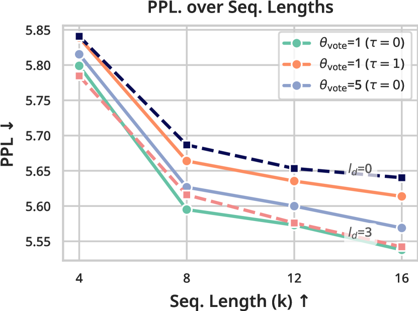
HiP Ensemble Performance. To show that ensemble enables end-to-end sub-quadratic complexity with comparable performance to our default HiP (), we compare full HiP (), default HiP (), and ensemble HiP with . We fix , that gave the best performance in , as shown in Fig. 13. The result indicates that HiP ensemble with , outperforms both full HiP and default HiP, as shown in Fig. 12 (Left). It shows notable improvements by decreasing 0.1 points of perplexity compared to full HiP () in most sequence lengths except the 4k. Since it also shows comparable performance to the HiP with dense layers, the ensemble could replace all the dense attention without any performance degradation.
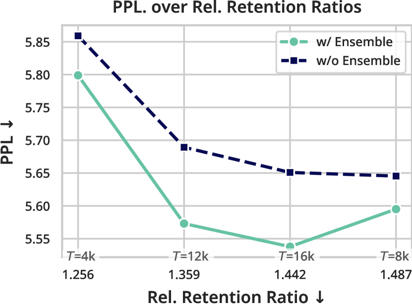
Moreover, we provide a comparison with full HiP () with the same sparsity as the ensemble to show such improvement is not simply because of the increased number of selected indices resulting from our ensemble method. As shown in Fig. 12 (Right), our ensemble method is Pareto frontier compared to HiP. Therefore, the ensemble can replace vanilla attention completely with HiP attention without any performance degradation, resolving challenges (1) and (2) in HiP if the computational cost is lower than the dense layer.
Latency of Ensemble. Since we sample multiple HiP masks by and perform voting operations across a large number of indices, we cannot guarantee that the HiP ensemble is always faster than vanilla attention in various sequence lengths. However, since the complexity of the HiP ensemble is still , the computational cost should be faster than vanilla attention at some point. Furthermore, in a later paragraph of the ablation study, we find out some hyper-parameters heavily adjust the retention ratio depending on sequence length or the hyper-parameter itself. This finding may indicate that the HiP ensemble might not be optimal for some sequence lengths and hyper-parameters. Therefore, the user must carefully investigate how the latency cross-over happened between vanilla and ensemble.
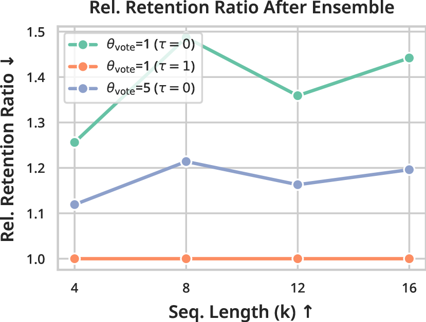
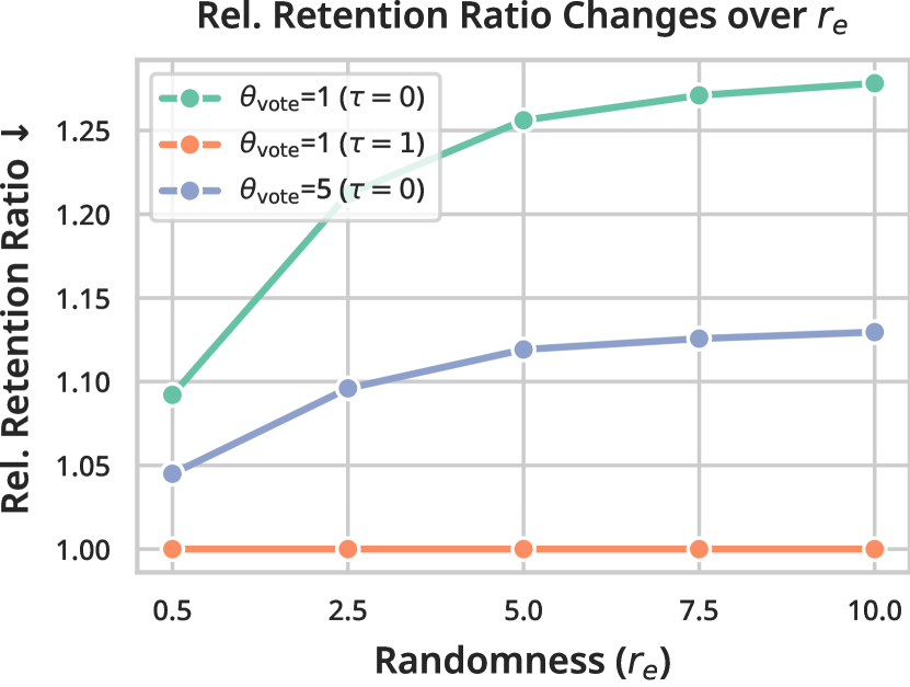
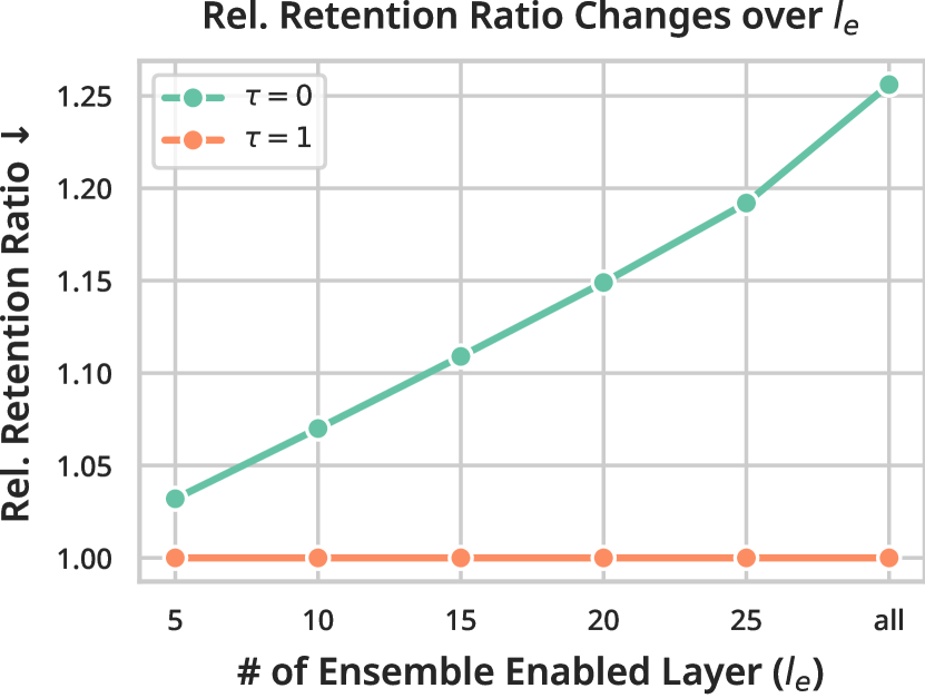
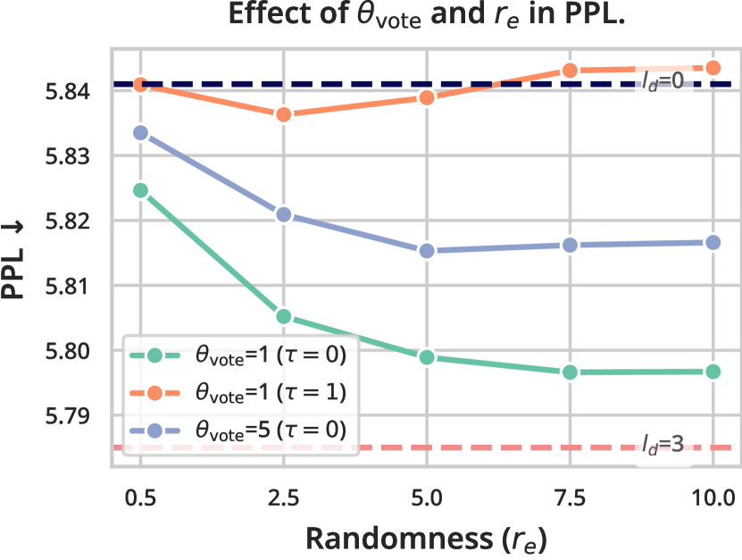
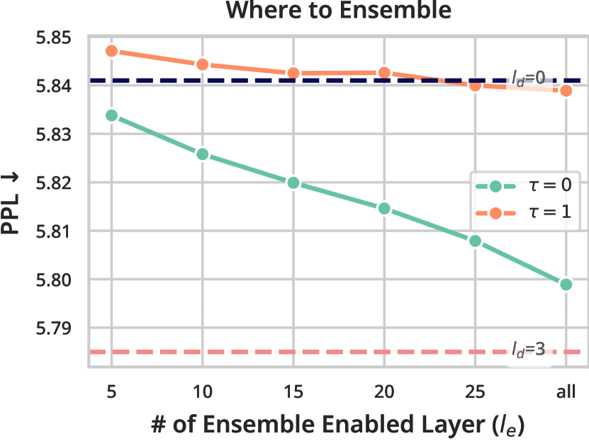
Ablation Study of Ensemble Hyper-parameter: , , , . As shown in Fig. 13 (Left), with , and gives the highest score. This indicates that performing the union operation with large randomness in sampling gives the highest performance. Also, in Fig. 13 (Right), with , we show that works the best, therefore if we want to replace the few layers of vanilla attention, then we would have to force every layer to enable ensemble.
Correlation Between the Relative Retention Ratio and Ensemble Factors. In Fig. 14, we show that the relative retention ratio shows no correlation with sequence length, while randomness shows a positive correlation. Moreover, when measuring the relative retention ratio changes over with , since we treat the ensemble disabled layer as having a 1.0 relative retention ratio, more ensemble-enabled layers to lead to a higher relative retention ratio.
E.3 Analysis with Visualization
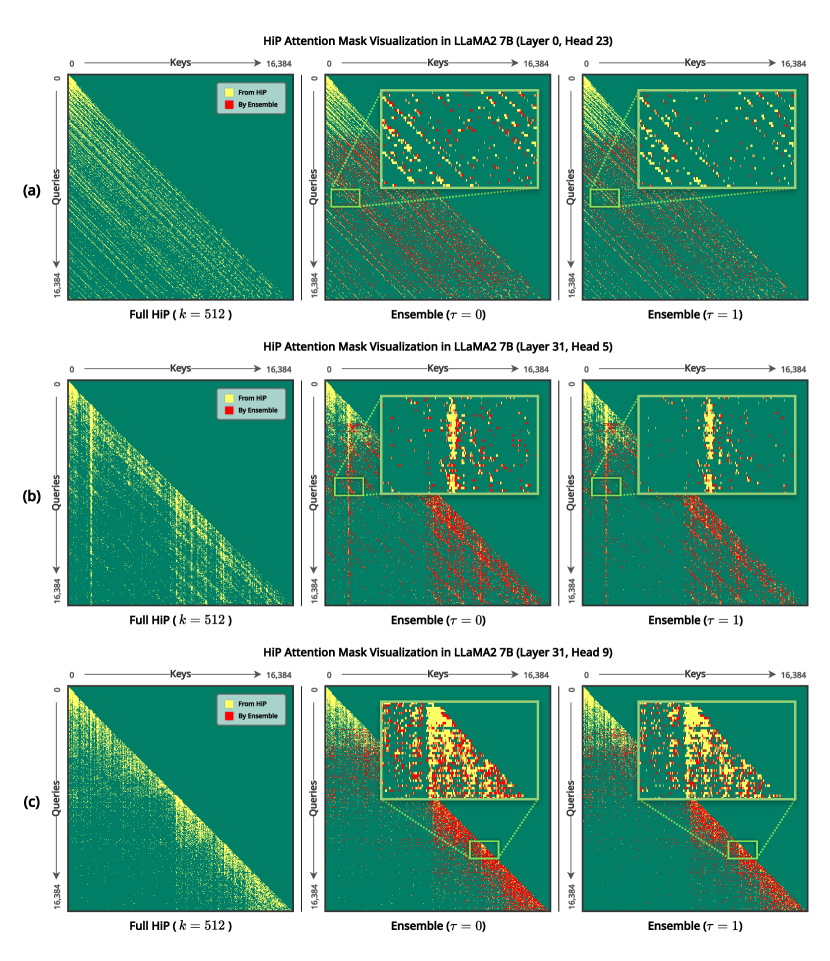
In Fig. 15, we provide a visual analysis to show how the ensemble selects indices that HiP missed to fill up a complete attention pattern and to show how it enables dynamic sparsity. We can see how the ensemble catches missed important indices such as diagonal, vertical, and stride attention patterns in (a), (b), and (c) of Fig. 15. This could be the critical reason for how the ensemble gave high performance in Fig. 12 by completing intuitive attention patterns, which are previously introduced as heuristics patterns in [4, 40]. Moreover, compared to HiP (left), we can see how the union operation (center) enables dynamic sparsity per head. Especially in (c), we can see that the ensemble is effective for filling missed indices in a long sequence while providing dynamic sparsity for each row (red pixels are gradually frequent in the bottom). Lastly, although in Fig. 12 we showed that (center) outperforms (right), in Fig. 15, we can see that still picks important indices from those that selected, given a restriction in the sparsity.
Appendix F Negative Social Impact
In this paper, we do not perform a careful investigation on LLM alignment performance with HiP. There is the potential that HiP might break the LLM safety guard. However, as far as we observed during the experiment, the HiP could preserve most of the behavior of trained LLM. Furthermore, we could always adopt the third-party LLM safety guard model such as LLaMA Guard [15].