Low algorithmic delay implementation of convolutional beamformer for online joint source separation and dereverberation
Abstract
Blind-audio-source-separation (BASS) techniques, particularly those with low latency, play an important role in a wide range of real-time systems, e.g., hearing aids, in-car hand-free voice communication, real-time human-machine interaction, etc. Most existing BASS algorithms are deduced to run on batch mode, and therefore large latency is unavoidable. Recently, some online algorithms were developed, which achieve separation on a frame-by-frame basis in the short-time-Fourier-transform (STFT) domain and the latency is significantly reduced as compared to those batch methods. However, the latency with these algorithms may still be too long for many real-time systems to bear. To further reduce latency while achieving good separation performance, we propose in this work to integrate a weighted prediction error (WPE) module into a non-causal sample-truncating-based independent vector analysis (NST-IVA). The resulting algorithm can maintain the algorithmic delay as NST-IVA if the delay with WPE is appropriately controlled while achieving significantly better performance, which is validated by simulations.
Index Terms— Independent vector analysis, weighted prediction error, non-causal sample truncating technique, algorithmic delay.
1 Introduction
Blind audio source separation (BASS) refers to the problem of separating audio source signals from observed mixtures with minimal prior information[1, 2, 3, 4]. Many methods have been developed to tackle this problem, among which the so-called independent vector analysis (IVA) [5, 6] has been widely investigated and has demonstrated promising separation performance. Originally, IVA-based algorithms are deduced to run on batch mode, and therefore large latency is unavoidable, which is unacceptable in most real applications. To achieve low latency, online versions of IVA are developed [7, 8, 9, 10]. This type of algorithms achieves separation on a frame-by-frame basis in the short-time-Fourier-transform (STFT) domain and the latency is significantly reduced as compared to those batch methods. However, the delay introduced by these algorithms may still be too long for many real-time applications since it depends on the frame length. The frame length in these algorithms has to be longer than the room impulse responses to achieve reasonably good separation performance.
To address this issue, a group of methods called convolutional beamformer (CBF) [12, 13, 14], which combine IVA and weighted prediction error (WPE) techniques [15, 16], is extended to the online version [17, 18, 19]. By integrating WPE, the CBF methods can process both current and past frames to mitigate the impact of reverberation even when the STFT frame length is short [17]. A drawback of this type of algorithms is that they are computationally expensive as the convolutional operation uses a number of frames to achieve dereverberation. In this work, we introduce a method that combines online CBF [17] and non-causal sample-truncating-based independent vector analysis (NST-IVA) [11]. This method uses a long STFT analysis window to reduce the length of convolutional operation in updating dereverberation filters while maintaining low algorithmic delay by truncating the non-causal samples of the process filters. Simulation results show that the proposed system is able to reduce the algorithmic delay to as low as ms while producing better separation performance than its conventional counterparts.
2 Non-causal sample-truncating-based IVA
2.1 Algorithmic delay description
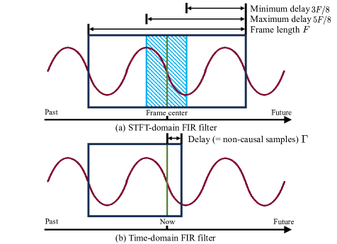
The algorithmic delay of the STFT- and time-domain algorithms is illustrated in Fig. 1. In the STFT-domain, due to the use of overlap-add technique, the output at time is affected by multiple frames. To clarify the discussion, we calculate the algorithmic delay of an output point from the frame with the closest center to it. For example, as illustrated in Fig. 1(a), if we assume that the frame size is and the overlap rate is , the algorithmic delay of the samples within the light blue box depends on the frame noted by the black box. The average delay of these samples is F/2 since STFT cannot be performed until all samples in this frame are received. In other words, the algorithmic delay of an STFT-domain filter is related to the analysis window length. In comparison, for the time-domain algorithms, as illustrated in Fig. 1(b), the algorithmic delay of the filter depends only on its non-causal sample number . If truncating the non-causal components of a time-domain filter is feasible, its algorithmic delay can be reduced.
2.2 Conventional online IVA algorithms
Suppose that there are sources in the sound field and we use an array of microphones to pick up the signals. The observation signals in the STFT domain can be expressed as
| (1) |
where
| (2) | ||||
| (3) |
are the observed and source signal vectors respectively, is the STFT bin index, is the time frame index, is the mixing matrix, and denotes the transpose operation. In this paper, we only consider the case with two microphones and two sources, i.e., . In our future work, we will investigate the causality of the separation filter with more input channels and apply this method to a larger microphone array. Assume that the matrix is of full rank, the source signals can be estimated with a linear filter, i.e.,
| (4) |
where is the separation matrix, is an estimate of the source signals vector.
The algorithmic delay in the STFT domain is bounded to the STFT frame length. One way to reduce the delay is through truncation [11]. By inverse discrete Fourier transform (IDFT), the separation matrix is converted back to the time domain as
| (5) |
where is the th element of , and corresponds to the time-domain FIR filter coefficient of th source, th input channel with the discrete-time index . Then, the separation process is expressed as
| (6) |
where is the time-domain estimated signal of th source at time , denotes the signal observed at the th microphone. As proved in [11], the ideal separation filter is a causal filter when . Hence, the algorithm delay can be reduced through truncation. Suppose that a total of non-causal samples are truncated, the separated signal is expressed as
| (7) |
The algorithm delay is then shortened from to .
3 Proposed method
3.1 System structure
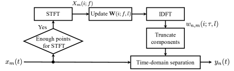
The flowchart of the proposed algorithm is shown in Fig. 2. To further improve the BASS performance in heavy reverberation while maintaining a low algorithmic delay, a parallel processing structure similar to the one in NST-IVA [11] is used. This structure updates the joint separation and dereverberation filters by the conventional online CBF in the STFT-domain [17]. After updating, the filters are transformed back to the time-domain to separate new observed signals directly.
3.2 Filters updating in the STFT domain
3.2.1 Problem formulation and probabilistic model
When the room impulse response is much longer than the STFT frame length, the instantaneous mixing model is not sufficient. Therefore, we adopt the convolutional transfer function (CTF) model in CBF [12, 13] to model the problem, i.e.,
| (8) |
where is the convolutional mixing matrix at time lag , and is the order of the mixing filters. Correspondingly, the convolutional filters are used for simultaneous dereverberation and separation, i.e.,
| (9) |
where is a filter with time lag , is the total orders of filters, and is a delay parameter introduced to prevent from distortion [15]. Based on the online source-wise factorization of CBF [17], the filters in (9) can be decomposed into the following two processes:
| (10) | ||||
| (11) |
The first process in (10) corresponds to the dereverberation process of the th source, where and are the dereverberation filter and the output signal, represents conjugate transpose and is the vector containing past samples of the mixture signals. The second process in (11) corresponds to the separation process, which uses filter to extract the th source signal. Substituting (10) and (11) into (9), we obtain the relation between and , , i.e., and , where is the th column of . Note that even though an STFT-domain separated signal component is produced in the updating process of , this component is not be transformed to the time-domain as the final separated signal.
To deal with the joint dereverberation and source separation problem, the CBF method assumes that the source signal in the STFT-domain follows a Gaussian distribution with zero mean and time-dependent variance , i.e.,
| (12) |
To estimate the adaptive filters to count for time-variant effects, the online version of CBF [17] adds a forgetting factor to the conventional CBF’s negative log-likelihood function as
| (13) |
where is the separation matrix, and is the unknown parameter set, , , and . Each parameter set can be updated iteratively using the coordinate ascent method [20].
3.2.2 Update of
3.2.3 Update of
3.2.4 Update of
If fixing other parameters, the cost function in (3.2.1) degenerates to the one used in the online AuxIVA. Hence, the separation matrix can be estimated through the iterative source steering (ISS)-based updating rules [22], which has been used in many IVA-based methods [9, 23, 24]. After initializing the separation matrix of the current frame , this matrix can be updated with an auxiliary vector as
| (21) |
This update process is repeated for . To continue the updating, needs to be calculated. By substituting (21) into (3.2.1) and fixing other parameters, the update rules of can be derived as
| (22) |
where is the th element of ,
| (23) |
is the weighted covariance matrix of the signal after dereverberation updated in an autoregressive manner [8] with a forgetting factor .
3.3 Time-domain implementation
To reduce the algorithmic delay, we convert the original STFT-domain convolutional filters back to the time domain as in the conventional NST-IVA. Then, once a new signal sample is accessible, the output signal is generated immediately without waiting for enough samples for the next STFT frame. The transformation of by IDFT can be expressed as
| (24) |
where is the th element of and corresponds to the time-domain FIR filter parameter. Since STFT is a linear process, the STFT-domain joint separation and dereverberation process in (9) is equal to the following time-domain processing:
| . | (25) |
where is the window shift length of the STFT in updating filters. Moreover, we consider the window function of the STFT with the discrete time index and rewrite the time domain processing (3.3) as
| (26) |
To reduce the algorithmic delay, the non-causal samples of the filter need to be truncated. If , all non-causal samples fall only in the separation filter ; so, in this work, we consider only truncating . Besides, since the first tap of the convolutional transfer function is equal to the instant separation matrix in online IVA [8] as shown in subsection 3.2, the causality of can be proved in a same way as [11]. Hence, the non-causal samples of can be truncated without suffering heavy performance degradation. Suppose that a total of non-causal samples are truncated, the proposed FIR filter process (3.3) can be written as
| . | (27) |
With this step, the algorithmic delay is shortened to samples as in NST-IVA.
4 Experimental evaluation
4.1 Experiment setup
The clean speech signals for simulations are taken from the ATR Japanese Speech Database [25]. Each mixed signal is generated with two source signals arbitrarily selected from two speakers from the database. If the source signal is less than s, it is concatenated with another selected source signal and truncated then so the overall length is s. The pyroomacoustics Python package [26] is used to simulate room impulse responses (RIRs) where the room boundary coefficients are controlled so that the room reverberation time, i.e., , is ms. We simulate a two-element microphone array with a spacing of cm to observe the signals. The proposed method is validated under two different pairs of incidence angles in the two-speaker scenarios: (°, °) and (°, °). For each condition, simulations with different mixed signals are performed and the average results are used for evaluation and comparison. The distance between the microphone array center and the sources is m. All signals are sampled at kHz.
Two conventional methods are used as the baseline systems: NST-IVA [11] (denoted as TD-IVA) and the STFT-domain online CBF [17] (denoted as FD-CBF). The proposed time-domain implementation of CBF is denoted as TD-CBF. Hann window is used as the analysis window in STFT and the overlap ratio is set to . The frame length, the number of truncated samples, and the corresponding algorithmic delay of the studied methods are shown in Table 1. The values of and in CBF are set to and for the case with -ms frame length while and for FD-CBF. Although setting a longer WPE filter length, i.e., a larger value of , can help achieve better performance when using shorter STFT windows, this would increase the computation cost. Therefore, we only used the same WPE filter length for comparison. The forgetting factor of IVA and WPE are set to and respectively. All simulations were conducted on a workstation powered by Intel Xeon E3-1505M.
The improvement of source-to-distortion ratio (SDR), source-to-interferences ratio (SIR), and sources-to-artifacts ratio (SAR) [27] are used as the metrics to evaluate the separation performance.
| Method | Window | Truncated | Algorithmic |
| length | points | delay | |
| TD-IVA (32 ms) | ms | ms | |
| FD-CBF (4 ms) | ms | ms | |
| TD-CBF (Proposed, 32 ms) | ms | ms | |
| TD-CBF (Proposed, 4 ms) | ms | ms |
4.2 Experiment result
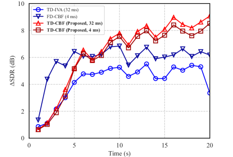
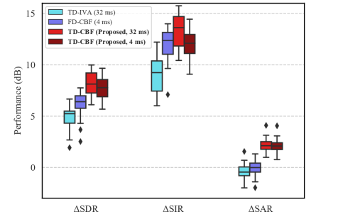
The SDR results as a function of time for all the studied methods are plotted in Fig. 3. As seen, all the studied methods converge at s. For a fair comparison of performance, we compute the average SDR, SIR, and SAR after all the methods converge, i.e., the results for the first -s are discarded. The results are shown in Fig. 4.
As seen in Fig. 3, FD-CBF with an ms analysis window takes only 3 seconds to converge while the other methods with a 64 ms analysis window take 6 seconds to converge. This shows that the methods converge slower with longer STFT window length than with shorter window length. According to this result, in practical systems, setting a relatively short window at the beginning and gradually increasing the length should be an appropriate way to achieve both good convergence speed and separation performance. From the results in Fig. 4, the proposed TD-CBF method (integrated with WPE dereverberation) yields much higher SDR, SIR, and SAR results than TD-IVA after convergence. In comparison with FD-CBF, the proposed method can maintain the same algorithmic delay ( ms) by truncating 448 non-causal samples, while using a relatively long STFT window length, which makes it more effective to deal with heavy reverberation. As a result, the proposed method also demonstrates better SDR, SAR than FD-CBF with the same algorithmic delay.
5 Conclusion
To achieve source recovery in reverberant environments with low latency, this paper developed an algorithm that combines the idea of non-causal sample truncation and WPE dereverberation method. Due to the application of non-causal sample truncation, the deduced algorithm is able to control the algorithmic delay as small as 4 ms. Meanwhile, due to the application of WPE, the algorithm is able to achieve better speech separation performance in strong reverberant environments in terms of source-to-distortion ratio and source-to-interferences ratio.
References
- [1] S. Makino, Audio Source Separation. Springer, 2018.
- [2] J. Benesty, I. Cohen, and J. Chen, Fundamentals of Signal Enhancement and Array Signal Processing. Wiley-IEEE Press., 2018.
- [3] G. Huang, J. Benesty, and J. Chen, “Fundamental approaches to robust differential beamforming with high directivity factors,” IEEE/ACM Trans. Audio, Speech, Lang. Process., vol. 30, pp. 3074–3088, 2022.
- [4] X. Wang, N. Pan, J. Benesty, and J. Chen, “On multiple input/binaural output antiphasic speaker signal extraction,” in Proc IEEE ICASSP, 2023, pp. 1–5.
- [5] T. Kim, I. Lee, and T.-W. Lee, “Independent vector analysis: Definition and algorithms,” in Proc. ACSSC, 2006, pp. 1393–1396.
- [6] A. Hiroe, “Solution of permutation problem in frequency domain ica, using multivariate probability density functions,” in Proc. ICA, 2006, pp. 601–608.
- [7] T. Kim, “Real-time independent vector analysis for convolutive blind source separation,” IEEE Trans. Circuits Syst. I, vol. 57, no. 7, pp. 1431–1438, 2010.
- [8] T. Taniguchi, N. Ono, A. Kawamura, and S. Sagayama, “An auxiliary-function approach to online independent vector analysis for real-time blind source separation,” in Proc IEEE HSCMA, 2014, pp. 107–111.
- [9] T. Nakashima and N. Ono, “Inverse-free online independent vector analysis with flexible iterative source steering,” in Proc. APSIPA ASC, 2022, pp. 749–753.
- [10] N. Ono, “Stable and fast update rules for independent vector analysis based on auxiliary function technique,” in Proc. IEEE WASPAA, 2011, pp. 189–192.
- [11] M. Sunohara, C. Haruta, and N. Ono, “Low-latency real-time blind source separation for hearing aids based on time-domain implementation of online independent vector analysis with truncation of non-causal components,” in Proc IEEE ICASSP, 2017, pp. 216–220.
- [12] T. Nakatani, C. Boeddeker, K. Kinoshita, R. Ikeshita, M. Delcroix, and R. Haeb-Umbach, “Jointly optimal denoising, dereverberation, and source separation,” IEEE/ACM Trans. Audio, Speech, Lang. Process., vol. 28, pp. 2267–2282, Jul. 2020.
- [13] T. Nakatani, R. Ikeshita, K. Kinoshita, H. Sawada, and S. Araki, “Computationally efficient and versatile framework for joint optimization of blind speech separation and dereverberation,” in Proc. Interspeech, 2020, pp. 91–95.
- [14] Y. Yang, X. Wang, A. Brendel, W. Zhang, W. Kellermann, and J. Chen, “Geometrically constrained source extraction and dereverberation based on joint optimization,” in Proc. EUSIPCO, 2023, pp. 41-45.
- [15] T. Nakatani, T. Yoshioka, K. Kinoshita, M. Miyoshi, and B.-H. Juang, “Speech dereverberation based on variance-normalized delayed linear prediction,” IEEE Trans. Audio, Speech, Lang. Process., vol. 18, no. 7, pp. 1717–1731, Sep. 2010.
- [16] T. Yoshioka and T. Nakatani, “Generalization of multi-channel linear prediction methods for blind mimo impulse response shortening,” IEEE Trans. Audio, Speech, Lang. Process., vol. 20, no. 10, pp. 2707–2720, Dec. 2012.
- [17] T. Ueda, T. Nakatani, R. Ikeshita, K. Kinoshita, S. Araki, and S. Makino, “Low latency online blind source separation based on joint optimization with blind dereverberation,” in Proc IEEE ICASSP, 2021, pp. 506–510.
- [18] T. Ueda, T. Nakatani, R. Ikeshita, K. Kinoshita, S. Araki, and S. Makino, “Low latency online source separation and noise reduction based on joint optimization with dereverberation,” in Proc. EUSIPCO, 2021, pp. 1000–1004.
- [19] T. Ueda and S. Makino, “Constant separating vector-based blind source extraction and dereverberation for a moving speaker,” in Proc. EUSIPCO, 2023, pp. 930–934.
- [20] T. Yoshioka, T. Nakatani, M. Miyoshi, and H. G. Okuno, “Blind separation and dereverberation of speech mixtures by joint optimization,” IEEE Trans. Audio, Speech, Lang. Process., vol. 19, no. 1, pp. 69–84, Jan. 2010.
- [21] P. S. Diniz et al., Adaptive filtering. Springer, 1997.
- [22] R. Scheibler and N. Ono, “Fast and stable blind source separation with rank-1 updates,” in Proc. IEEE ICASSP, 2020, pp. 236–240.
- [23] K. Goto, T. Ueda, L. Li, T. Yamada, and S. Makino, “Geometrically constrained independent vector analysis with auxiliary function approach and iterative source steering,” in Proc. EUSIPCO, 2022, pp. 757–761.
- [24] K. Mo, X. Wang, Y. Yang, T. Ueda, S. Makino, and J. Chen, “On joint dereverberation and source separation with geometrical constraints and iterative source steering,” in Proc. APSIPA ASC, 2023, pp. 1138–1142.
- [25] A. Kurematsu, K. Takeda, Y. Sagisaka, S. Katagiri, H. Kuwabara, and K. Shikano, “ATR japanese speech database as a tool of speech recognition and synthesis,” Speech communication, vol. 9, no. 4, pp. 357–363, 1990.
- [26] R. Scheibler, E. Bezzam, and I. Dokmanić, “Pyroomacoustics: A python package for audio room simulation and array processing algorithms,” Proc. IEEE ICASSP, 2018, pp. 351–355.
- [27] E. Vincent, R. Gribonval, and C. Févotte, “Performance measurement in blind audio source separation,” IEEE Trans. Audio, Speech, Lang. Process., vol. 14, no. 4, pp. 1462–1469, Jun. 2006.