Faster Convergence on Heterogeneous Federated Edge Learning: An Adaptive Sidelink-Assisted Data Multicasting Approach

Abstract

Federated Edge Learning (FEEL) emerges as a pioneering distributed machine learning paradigm for the 6G Hyper-Connectivity, harnessing data from the Internet of Things (IoT) devices while upholding data privacy. However, current FEEL algorithms struggle with non-independent and non-identically distributed (non-IID) data, leading to elevated communication costs and compromised model accuracy. To address these statistical imbalances within FEEL, we introduce a clustered data sharing framework, mitigating data heterogeneity by selectively sharing partial data from cluster heads to trusted associates through sidelink-aided multicasting. The collective communication pattern is integral to FEEL training, where both cluster formation and the efficiency of communication and computation impact training latency and accuracy simultaneously. To tackle the strictly coupled data sharing and resource optimization, we decompose the overall optimization problem into the clients clustering and effective data sharing subproblems. Specifically, a distribution-based adaptive clustering algorithm (DACA) is devised basing on three deductive cluster forming conditions, which ensures the maximum sharing yield. Meanwhile, we design a stochastic optimization based joint computed frequency and shared data volume optimization (JFVO) algorithm, determining the optimal resource allocation with an uncertain objective function. The experiments show that the proposed framework facilitates FEEL on non-IID datasets with faster convergence rate and higher model accuracy in a limited communication environment.

I Introduction

In modern wireless networks, the proliferation of advanced sensors has engendered a significant surge in data generation, spanning diverse modalities such as texts, images, videos, and audio streams [2]. This influx of big data is conventionally offloaded and stored on cloud platforms, often coupled with Artificial intelligence (AI) techniques to facilitate a series of intelligent services. However, the privacy leakage problem becomes critical when considering the exposure of sensitive raw data to potential attacks and cyber threats, especially after certain legislations on data privacy are introduced, e.g., the General Data Protection Regulation (GDPR) [3]. This predicament causes data owners to become increasingly privacy-sensitive and hesitant to share their data. As a solution, a novel distributed learning paradigm, termed Federated Learning (FL), has been introduced to construct a high-quality model by leveraging locally-trained models instead of directly sharing raw local data [4].

In the FL framework, a number of federated rounds are required between clients and servers to collaboratively achieve desired accuracy [4, 5, 6]. Given the nature of deep learning models containing millions of parameters, e.g., the Large Language Model (LLM) GPT-3.5 has 175 billion parameters [7], transmitting such high-dimensional models results in a substantial communication costs. By balancing communication and computation resources of edge devices, Federated Edge learning (FEEL) has been proposed to reduce latency and energy consumption in wireless networks [8]. Yet the training costs are still serious especially when training with non-independent and non-identically distributed (non-IID) data across devices in FEEL. In practice, due to the decentralized and geographically dispersed nature of edge devices, data within a federated learning environment displays significant variations and samples imbalance, i.e., statistical heterogeneity. Extensive research studies [9, 10, 11, 12] have shown that as the degree of heterogeneity increases, the convergence of the FEEL algorithm slows down, and more communication rounds are required for the desired accuracy. Therefore, the time consumption and weak accuracy caused by the non-IID data become the bottleneck of FEEL applied in real-world IoT applications.

There is plenty of research trying to solve the statistical heterogeneity problem, which can be categorized into two types: 1) model-driven and 2) data-driven [13]. The model-driven methods refer to designing the internal structure and parameters of the models to mitigate performance loss. Li et al. [14] adds a proximal term to the local loss function to constrain the distance between the local model and the global model. [15] and [16] correct the update drift in local training and provide convergence guarantees for non-IID FL. Instead of training a single global model with well generalization, [17, 18, 19] aim at grouping the client into clusters and training personalized models based on data distribution. These works assume that there is intra-cluster similarity and inter-cluster dissimilarity in clients’ data distributions. [20] and [21] provide the different model structures for heterogeneous clients by knowledge distillation techniques. Data-driven approaches manipulate and augment the local data to make distribution more homogenous. Zhao et al. [5, 11, 22], develop a method that shares a small subset of local data with all devices to improve model accuracy. [23] and [24] propose a hybrid learning mechanism wherein the server collaboratively trains the model with an approximately IID dataset uploaded from the clients. [20] employs GAN technology to ensemble data information in a data-free manner, broadcasting the generator to all users and regulating local updates to mitigate bias. Both approaches entail sacrificing additional communication or computational resources in order to achieve accuracy improvements.

To mitigate the communication cost, some other studies try to design resource-efficient FEEL system. These approaches aim to minimize FL loss while optimizing resource efficiency. Unfortunately, these two goals largely conflict with each other, as obtaining a higher-quality model often necessitates increased resource consumption, and vice versa. Chen et al. [25] introduce a joint learning and communication framework that derives a closed-form expression for convergence based on packet error rates, and formulates optimal strategies for user selection and resource allocation to minimize the FEEL loss function. Zhao et al. [11] jointly minimizes the accuracy loss and the cost of data sharing to mitigate the impact of non-IID data, and proposes a computation-efficient algorithm to approach a stationary optimal solution. [26] proposes a resource-efficient method for training a FL model with non-IID data, effectively minimizing cost through an auction approach and mitigating quality degradation through data sharing. [9] analyzes the implicit connection between data distribution and trained models from empirical and mathematical perspectives, and proposes a reinforcement learning-based mechanism for selecting the optimal subset of devices. Therefore, it is a majority challenge for FEEL to accelerate training process in communication and computation meanwhile ensuring model performance with non-IID data.

Although these approaches have attempted to address the statistical heterogeneity issue at model-driven, data-driven, and system design levels, deploying non-IID FL in wireless communication systems still faces challenges. Firstly, model-driven methods demand additional computing resources and show marginal improvements. The increased complexity of local training adds to the difficulty of applying FL in resource-constrained wireless networks. Much work [26, 5, 11, 23] demonstrate that data sharing is a straightforward and efficient method for directly mitigating model quality degradation. Secondly, most data sharing methods work under the strongly assumption of a publicly available proxy data source on the server side [21, 26]. However, building a pre-processed and labeled public dataset is a time-consuming and expensive task. Evaluating the quality of the shared dataset is also critical, since it directly ensures performance gains. Lastly, the costs and privacy concerns of data sharing cannot be ignored. Exchanging data unavoidably raises information leakage, additional latency, and energy consumption. Specifically, when an excessive amount of data is transferred, the costs and privacy risks may outweigh the benefits of sharing data.

Based on the above analysis, this work proposes a data sharing framework that allows partial data exchanged among trusted user groups to reduce the degree of data heterogeneity. In the real-world scenario, there are certain devices with high-quality data that can accelerate FEEL training. By the aid of the high-bandwidth mmWave multicasting technology [27], these nodes can share the private data with trustable neighbors in close proximity communication (i.e., sidelink) directly without going through the base station (BS). These sidelink transmissions boost network ulity while saving spectrum resource since it enables the simultaneous delivery of content to multiple users through a single transmission [28]. By selectively exchanging data with trustworthy and dependable partners via sidelink-aided technology, communication overhead and privacy concerns can be effectively regulated. Moreover, the goals of this paper are not only to mitigate the statistical heterogeneity issue, but also to accelerate FEEL training by exploiting data and computility of edge network. The key contributions of this paper are summarized as follows:

• Clustered data sharing FEEL framework for eliminating statistical heterogeneity: Inspired by the valid results of data-driven methods on non-IID FL, we propose a clustered data sharing framework which can evaluate and eliminate the impacts of statistical heterogeneity. Sidelink-aided multicasting is used as an enabling technology of wireless network for FL to achieve faster training and higher accuracy. Moreover, this framework can serve as a data preparation procedure applicable to model-driven non-IID FL algorithms.

• Fast convergence with joint communication, computation configuration: An optimization problem is formulated to minimize the overall delay of the FL task with clustered data sharing by jointly considering communication, computation, and privacy. Here, devices are allowed to trustfully cluster and exchange data to accelerate FEEL training convergence. The shared data volume and computed frequency are jointly optimized to achieve trade-off among sharing delay, communication delay, and computation delay over the training rounds.

• An innovative low-complexity clustering algorithm utilizing constrainted graph for no closed-form problem: By quantifying the statistical heterogeneity, the minimization delay problem is transformed into minimizing the distribution distance while adhering to privacy and communication requirements. We theoretically analyze this intractable problem from individual, intra-cluster, and inter-cluster perspectives. Subsequently, by transforming the original subproblem into a constrained graph, we devise a clustering method named distribution-based adaptive clustering algorithm (DACA) to facilitate efficient cluster formation.

• A SSCA optimization algorithm for computed frequency and shared data volume allocation problem: Due to the uncertain gain of data sharing on training round, the objective function with respect to shared data volume is non-closed form. Through theoretical convergence analysis, we provide a functional relationship that captures the relationship between data distribution and convergence rate. Then we employ the stochastic successive convex approximation (SSCA) algorithm to solve the nonconvex optimization problem with estimated parameters. Through solving the surrogate problem iteratively, the proposed joint computed frequency and shared data volume optimization (JFVO) algorithm is guaranteed to convergence to a stationary solution.

• Performance evaluation from various perspectives: Our proposed approaches are evaluated by applying classic image classification tasks to the MNIST and CIFAR-10 datasets. The clustered data sharing FL with DACA can effectively improve the accuracy in different non-IID cases and significantly reduce the total training task delay. Moreover, The experimental results shows that the proposed JFVO algorithm can convergence in different communication states.

The rest of this paper is structured as follows: Section II explores and analyzes the FL performance with heterogeneous data. Section III presents a clustered data sharing FL framework over wireless networks. Section IV formulates a problem aiming to minimize delays while mitigating the impact of non-IID data, and a joint optimization algorithm is designed to make a good tradeoff between the performance improvement and the cost. Section V provides the numerical results, and finally conclusions are drawn in Section VI.

II Federated learning with non-IID data

In this section, we provide a comprehensive definition of non-IID data in federated learning, which is also referred to as “statistical heterogeneity”. We first introduce the classification of non-IID data distribution, and then apply the statistical distance to generally quantify the heterogeneity. Based on the preliminary experiments on the non-IID FL, a clustered data sharing method is proposed to address the non-IID challenge of FL without requiring extra datasets.

II-A Statistical Heterogeneity

The local data generated at clients is statistically different, and may vary significantly, resulting in the typical non-IID cases. To illustrate this, consider a supervised learning task with input features $\mathbf{x}$ and labels $y\in\left\{{1,...,Y}\right\}$. The statistical model of learning involves sampling the example-label pairs from the local data distribution of the client $k$, i.e., $\left({{\mathbf{x}},y}\right)\sim{{P}_{k}}\left({{\mathbf{x}},y}\right)$. If all local samples follow the same global distribution ${{P}_{g}}$ and are independent of each other, this is defined as IID in statistics, which has a mathematic form $\left({{\mathbf{x}},y}\right)\sim{{P}_{g}}\left({{\mathbf{x}},y}\right)$. Nevertheless, as users predominantly possess only localized data constrained by geo-regions and observation ability, the FL violates the IID assumption, resulting in distinctions between ${{P}_{i}}$ and ${{P}_{j}}$ for different clients $i$ and $j$. We survey the following different cases for the non-IID assumption and rewrite ${{P}_{k}}({\mathbf{x}},y)$ as ${{P}_{k}}(y\left|{\mathbf{x}}\right.){{P}_{k}}({\mathbf{x}})$ or ${{P}_{k}}({\mathbf{x}}\left|y\right.){{P}_{k}}(y)$ allows us to characterize these different cases more precisely.

Label distribution skew: The marginal distribution ${{{P}}_{k}}(y)$ may vary across clients, even if ${{{P}}_{k}}({\mathbf{x}}\left|y\right.)$ is the same, e.g., some labels only appear to a few users but not others.

Feature distribution skew: The marginal distribution ${{{P}}_{k}}({\mathbf{x}})$ may vary across clients, even if ${{{P}}_{k}}(y\left|{\mathbf{x}}\right.)$ is the same, e.g., handwriting with the same label may vary in personal style.

Including the two common non-IID cases above, there are several other categories of distribution skews: Concept shift refers to the same label ${{{P}}_{k}}(y)$ with different features ${{{P}}_{k}}({\mathbf{x}}\left|y\right.)$ or the same feature ${{{P}}_{k}}({\mathbf{x}})$ with different labels ${{{P}}_{k}}(y\left|{\mathbf{x}}\right.)$. Quantity skew refers to the situation where the amount of data available for training differs significantly among participating clients.

Similar to the majority of non-IID FL works, our work also focuses on label distribution skew, and can be extended to feature distribution skew and other cases.

II-B Quantify Heterogeneity

The evaluation of the distribution skewness is the first step for data owners and the FL server to explore the impact of non-IID data on training. The earth mover’s distance (EMD) is generally applied as a metric to quantify non-IIDness between the local dataset and the global dataset. Specifically, given the local label distribution ${{{P}}_{k}}(y)$ and the global label distribution ${{{P}}_{g}}(y)$, the EMD of client $k$ can be calculated by

$${D_{{\text{EMD}}}}\left(k\right)=\sum\limits_{i=1}^{Y}{\left\|{{{P}_{k}}\left({y=i}\right)-{{P}_{\text{g}}}\left({y=i}\right)}\right\|}.$$ (1)

There are also some other commonly used methods to measure the statistical distance, e.g., KL divergence [29] and JS divergence [30]. However, EMD is more widely applied in non-IID research [5, 31, 32], because it can more accurately capture the impact of statistical heterogeneity on model training [5].

Intuitively, the impact of non-IID data can be portrayed by the deviation between the model $w_{g}$ trained on the non-IID dataset and ${w_{{\rm{IID}}}}$ trained on the IID dataset. As model training is data-dependent, it can be inferred that the distance between data distributions can be used to measure the weight divergence $\left\|{{w_{g}}-{w_{{\rm{IID}}}}}\right\|$. Fortunately, some existing works have theoretically shown that ${D_{{\text{EMD}}}}$ is the root cause of the weight divergence [5, 9], i.e., $\left\|{{w_{g}}-{w_{{\text{IID}}}}}\right\|\propto{D_{{\text{EMD}}}}\left(k\right)$, and hence, $D_{{\text{EMD}}}\left(k\right)$ is an appropriate metric for non-IID FL. Moreover, we define the weighted sum of separate EMD values as the average EMD to reflect the overall data skewness:

$${{\bar{D}_{{\rm{EMD}}}}=\sum\limits_{k=1}^{K}{\frac{{{n_{k}}}}{n}\sum\limits_{i=1}^{Y}{\left\|{{{P}_{k}}\left({y=i}\right)-{{P}_{g}}\left({y=i}\right)}\right\|}}},$$ (2)

where $n_{k}$ is the number of samples in client $k$, and $n=\sum\nolimits_{k=1}^{K}{{n_{k}}}$ is the total number of samples across all $K$ clients. Note that the EMD can also be applied to quantify feature distribution skew and other cases by replacing different distribution expressions.

II-C Preliminary Experiments and Analysis

(a) Impact of different non-IID degrees

(b) Impact of shared data volume

(c) Impact of number of clusters

Figure 1: Train loss on clustered data sharing for non-IID FL. (a) For IID setting, each user is randomly assigned a uniform distribution over all classes. For non-IID setting, the proportion of labels of among users are different, leading to varying ${\bar{D}_{{\text{EMD}}}}$. (b) The shared data volume is quantified as $\alpha$, representing the proportion of sharing data volume in its local data volume. (c) The users are randomly divided into clusters, where each cluster consists of cluster heads to transmit data and cluster members to receive data.

To mitigate the divergence between the local and global distributions, one possible approach is to share data among the participating clients. Traditional data sharing schemes involve a centralized server sharing a portion of the global data, which is made available to all clients. However, this approach requires the creation of a publicly accessible proxy data source, which can be impractical or pose privacy concerns. Instead of centralized sharing, we randomly select clients to exchange local data within clusters. The preliminary experiments between this scheme and the standard FedAvg algorithm reveal that the convergence of the training process is impacted by three main factors.

Degree of heterogeneity: reflects the skewness value of all local data distributions in the overall system, i.e., ${\bar{D}_{{\text{EMD}}}}$. To further investigate the relationship between degree of heterogeneity and FL training performance, we lay out the experiment on the training loss of non-IID FL with different ${\bar{D}_{{\text{EMD}}}}$ settings. As shown in Fig. 1a, it is clear from the result that with the decrease in data heterogeneity, the convergence rate of the FL training is significantly improved, and the loss value of training becomes lower.

Shared data volume: refers to how much data is transmitted to the clients. Sharing little data is ineffective for FL training, and much more data would increase the communication burden. To investigate the gains and costs of data sharing, we conduct the second experiment on clustered sharing with different shared data volumes. As shown in Fig. 1b, as the volume of shared data increases, the convergence rate of FL also increases. Furthermore, it is worth noting that the convergence improvement achieved by raising the shared data volume from $\alpha=0.05$ to $\alpha=0.1$ is not as significant as from $\alpha=0$ (without data sharing) to $\alpha=0.05$.

Number of clusters: plays a critical role in determining the effectiveness of the data sharing scheme. Increasing the number of clusters can reduce transmission costs but may not be beneficial for FL training. As shown in Fig. 1c, it can be observed that excessive clustering can have a negative impact on FL performance instead of improving it when comparing the cases of clusters $=10$ with clusters $=25$. Too many clusters may result in data sharing being inefficient, and random data sharing itself can not always guarantee performance gains and can incur communication costs.

Based on the experiments and analyses presented above, several notable conclusions can be drawn:

1. The lower skewness datasets converge faster during training and achieve higher accuracy, which can be characterized by the lower average-EMD between the data distributions.

2. The benefits of data sharing increase as the shared data volume rises, but the rate of improvement is diminishing. In particular, when the transmitter shares an excess of data, the cost of data sharing becomes the critical bottleneck for FL training instead of heterogeneity. Therefore, it is important to make the trade-off between data sharing and FL training.

3. The effectiveness of clustered data sharing depends on the clustering strategy. Combined with item 1 above, it is clear that an efficient clustering method for accelerated non-IID FL does not depend on the number of clusters but on the contribution to the average EMD ${\bar{D}_{{\rm{EMD}}}}$.

In conclusion, it is critical to design a reasonable clustering method to accelerate federated learning with acceptable sharing delay, i.e., minimizing the total delay of data sharing and FL training.

III System Model

Consider a wireless edge computing system consisting of a BS and a set of $K$ users (i.e., smart mobile devices) denoted as ${\cal K}=\{1,2,...,K\}$. Each user collects the local samples ${{{\cal N}}_{k}}=\{{\bf{x}}_{i}^{k},y_{i}^{k}\}_{i=1}^{{n_{k}}},\;k\in{{\cal K}}$, where ${\bf{x}}_{i}^{k}$ is the input vector of sample $i$, $y_{i}^{k}$ is the corresponding labels, and ${n_{k}}$ is the number of the sample-label pairs. The collaborative interaction between users and the BS is facilitated within a client-server architecture to accomplish intelligent services, e.g., computer vision tasks. In this edge environment, besides the conventional downlink/uplink transmission between clients and the server, sidelink-assisted multicasting are enabled for users in close proximity.

Figure 2: Clustered data sharing framework for FEEL.

III-A Clustered Data Sharing FEEL Framework

To relieve the data imbalance feature for FL, we propose a communication-aware clustered data sharing scheme which makes data distributions more homogeneous among devices by exchanging a small data subset within a communication-efficient and privacy-preserving cluster. As shown in Fig. 2, this framework consists of the following two stages.

The data preparing stage: involves a data augmentation procedure before the FEEL training. In this stage, all users are clustered with respect to data distribution, communication states, and privacy requirements, where each cluster is defined by a cluster $m$ and its corresponding cluster members ${{\cal C}_{m}}$. Then the cluster heads, denoted as the set ${\cal M}$, share the subsets of their data with cluster members through reliable multicast communication. Following clustered data exchange, each node can compute its local parameters with the mixed samples in the next stage. It is noted that each node cannot participate in more than one cluster to prevent conflicts, i.e., ${{\cal C}_{m}}\cap{{\cal C}_{l}}=\emptyset,\forall m,l\in{\mathcal{M}},m\neq l$. With a copy of shared data, the local data volume on device $k$ is then determined by the following expression:

$${{\tilde{n}_{k}}=\left\{\begin{array}[]{l}{n_{k}}+n_{m}^{s},\;\;k\in{{\cal C}_{m}},\;\forall m\in\mathcal{M},\\ {n_{k}},\quad\quad\quad\,{\rm{}}k\notin{{\cal C}_{m}},\;\forall m\in\mathcal{M},\end{array}\right.}$$ (3)

where $n_{m}^{s}$ is the data volume of sharing from cluster head $m$. Without loss of generality, we specify ${P_{m}}\left(y\right)={P_{k}}\left(y\right)$ if $k\notin{{\cal C}_{m}}$. The new data distribution on device $k$ can be derived as follows:

$${{\tilde{P}_{k}}\left(y\right)=\frac{{{n_{k}}{P_{k}}\left(y\right)+n_{m}^{s}{P_{m}}\left(y\right)}}{{{n_{k}}+n_{m}^{s}}}}.$$ (4)

Intuitively, clustered data exchange alters the original data distribution on each device, diluting the disparity in data features. Therefore, the value of the average EMD after data sharing is given by

$${{\tilde{D}_{{\rm{EMD}}}}=\sum\limits_{k=1}^{K}{\frac{{{{\tilde{n}}_{k}}}}{n}\sum\limits_{i=1}^{Y}{\left\|{{{\tilde{P}}_{k}}\left({y=i}\right)-{P_{g}}\left({y=i}\right)}\right\|}}}.$$ (5)

The FEEL training stage: is to train a global model via collaborations between the edge server and multiple clients, where the global model is obtained by minimizing the following loss function:

$${\mathop{\min}\limits_{{w_{g}}}\frac{1}{K}\sum\limits_{k=1}^{K}{\frac{1}{{{n_{k}}}}\sum\limits_{i=1}^{{n_{k}}}{{F_{k}}\left({{\bf{x}}_{i}^{k},y_{i}^{k},{w_{g}}}\right)}}}.$$ (6)

Here, ${F_{k}}\left(\cdot\right)$ represents the loss of prediction on the local sample $\left\{{\bf{x}}_{i}^{k},y_{i}^{k}\right\}$. Specifically, the model undergoes the following steps for updating during the $t$-th round:

i) Global Model Broadcast: The server broadcasts the global model ${w_{g}^{t-1}}$ to participants, updating their local models to ${w_{k}^{t}}$.

ii) Local Model Update: Participants independently train their local models $w_{k}^{t}$ using their respective datasets $\left\{{{\bf{x}}_{i}^{k},y_{i}^{k}}\right\}_{{\rm{i=1}}}^{{n_{k}}}$ via stochastic gradient descent (SGD) [33]: ${w_{k}^{t}}\leftarrow{w_{k}^{t}}-\eta\nabla{F_{k}}\left({{x_{i}},{y_{i}};{w_{k}^{t}}}\right)$ where $\eta$ is the learning rate in SGD, and $\nabla{F_{k}}\left(\cdot\right)$ is the gradient of the loss function ${F_{k}}\left(\cdot\right)$ with respect to $w_{k}^{t}$.

iii) Parallel Upload: After local updates, participants transmit $w_{k}^{t}$ to the BS via wireless cellular links.

iv) Synchronous Aggregation: Once all participants have completed local model transmission, the global model $w_{g}^{t}$ is updated by weighted-averaging the uploaded models:

$${w_{g}^{t}=\sum\limits_{k=1}^{K}{\frac{{{n_{k}}}}{n}w_{k}^{t}}}.$$ (7)

After model aggregation, $w_{g}^{t}$ is fed back to the devices, and the FEEL above training procedure repeats for multiple rounds until convergence.

III-B Clustered Data Sharing Model

As is well-known, data sharing is inherently associated with privacy risks and additional communication costs. To effectively mitigate these effects, two key metrics are defined for the further development and refinement of the cluster algorithm.

Social closeness: is one of the factors of social awareness, representing users with different levels of trust in each other [34]. Regarding data privacy, users’ reluctance to expose data is weakened in close social relationships. For clustered data sharing, we define the social closeness ${e_{m,c}}$ between the cluster head $m\in M$ and cluster member $c\in{{\cal C}_{m}}$. To ensure trustworthy data exchange, cluster members are required to maintain a socially closed affiliation with the cluster head, i.e., ${e_{m,c}}\geq{e_{{\rm{th}}}},\forall m,c$. For clarity, we build a graph ${{\cal G}}=\left({{{\cal K}},{{\cal E}}}\right)$ to illustrate the social closeness among users, where ${{\cal E}}=\{{e_{k,j}}\in\left[{0,1}\right],\forall k,j\in{{\cal K}}\}$ represents the set of graph edges [35].

Multicasting delay: The cluster head shares part of the datasets with the group members via sidelink-assisted multicasting. Sidelink is a technology in 5G/6G allowing for Device-to-Device (D2D) communication without using BS [27]. Then the general formulation of Signal to Interference and Noise Ratio (SINR) $\gamma$ is given by

$${\gamma\left({{d_{m,c}}}\right)=\sum\limits_{i=0}^{3}{\frac{{{C_{i}}A_{i}^{-1}d_{m,c}^{-{\zeta_{i}}}{\kappa_{i}}\left({{d_{m,c}}}\right){S_{F,i}}{U_{F,i}}}}{{{N_{0}}W+I}}}},$$ (8)

where ${C_{i}}={P_{m}}{G_{m}}{G_{c}}$, and $P_{m}$ is the transmit power, $G_{m}$ and $G_{c}$ are the antenna array gains at cluster head $m$ and member $c$. $d_{m,c}$ denotes the three-dimensional (3D) distance between cluster head $m$ and member $c$. ${\kappa_{i}},i\in\left\{{0,1,2,3}\right\}$ is the state probabilities of four states: non-line-of-sight (nLoS) with blocked, line-of-sight (LoS) with blocked, nLOS with non-blocked, LOS with non-blocked. $A_{i}$ and $\zeta_{i}$ are propagation coefficients of the path loss, which corresponding to the introduced states. ${S_{F,i}}$ and ${U_{F,i}}$ are state-dependent shadow and small-scale fading, $I$ is the interference. In the urban microcell (UMi) scenario, we set these coefficient values according to the 3GPP standards [36]. With multicasting, the transmission rate of data sharing within one cluster is determined by the worst sidelink, i.e.,

$${v_{m}^{s}=\mathop{\min}\limits_{c\in{\mathcal{C}_{m}}}\left\{{B_{m}^{s}{{\log}_{2}}\left({1+\gamma\left({{d_{m,c}}}\right)}\right)}\right\}},$$ (9)

Meanwhile, the total data sharing time cost ${\tau^{s}}$ depends on the maximal delay of clusters, and is thereby given by

$${{\tau^{s}}=\mathop{\max}\limits_{m\in\mathcal{M}}\left\{{\frac{{an_{m}^{s}}}{{v_{m}^{s}}}}\right\}},$$ (10)

where $a$ denotes bits of each data sample. The energy consumption of one-shot data sharing can be ignored compared to the multi-round FEEL training process.

III-C FEEL Transmission and Computation Model

As introduced in Section III-A, the FEEL training stage comprises four steps in each round, with each step incurring either communication or computational cost.

i) Broadcasting: The downlink transmission rate of the BS when broadcasting the global model to user $k$ can be expressed as follows:

$${v_{k}^{d}={B^{d}}{\log_{2}}\left({1+\frac{{{P_{{\text{BS}}}}{\left|h_{k}\right|}^{2}}}{{{I^{d}}+{B^{d}}{N_{0}}}}}\right)},$$ (11)

where ${B^{d}}$ is the bandwidth used by the BS to broadcast to global model; ${P_{{\text{BS}}}}$ is the transmit power of the BS, and ${h_{k}}$ is the channel gain between the BS and user $k$; $I^{d}$ represents the interference caused by other BSs which are not participating in training. As the channel state fluctuates during the downloading process, maintaining a constant transmission rate is infeasible. Thus, we employ the expected value of the transmission time cost to represent the true value. The corresponding downloading delay can be expressed as

$${\bar{\tau}_{k}^{d}={\mathbb{E}_{{h_{k}}}}\left({\frac{{M\left({{w_{g}}}\right)}}{{v_{k}^{d}}}}\right)},$$ (12)

where function $\mathbb{E}_{{h_{k}}}\left(\cdot\right)$ is the expectation with respect to $h_{k}$ and function $M\left(\cdot\right)$ is the model size of model $w_{g}$ in bits.

ii) Local computation: Assuming that $f_{k}$ denotes the computation capacity of user $k$ (measured in CPU cycles per second), The computation latency at user $k$ needed for data processing can be expressed by

$${\tau_{k}^{cop}=\frac{{{L_{k}}E{{\tilde{n}}_{k}}}}{{{f_{k}}}}}.$$ (13)

Here, $L_{k}$ denotes the number of CPU cycles needed for training per sample at user $k$. $E$ is the number of local epochs used in SGD updateing, indicating the number of times the local device iterates over its own subset of training data ${\tilde{n}}_{k}$. The energy consumption of each user $k$ for local model training can be expressed by

$${\gamma_{k}^{cop}={\varsigma}{L_{k}}E{{\tilde{n}}_{k}}f_{k}^{2}},$$ (14)

where $\varsigma$ is the energy consumption coefficient depending on the hardware of the devices.

iii) Uploading: After local computation, all users upload their local model parameters to the BS via orthogonal frequency division multiple access (OFDMA). The achievable uploading rate of user $k$ can be expressed as

$${v_{k}^{u}={B^{u}}\sum\limits_{i=1}^{R}{{r_{i,k}}}{\log_{2}}\left({1+\frac{{{P_{k}}{\left|h_{k}\right|}^{2}}}{{I_{k}^{u}+B_{k}^{u}{N_{0}}}}}\right)},$$ (15)

where $B_{k}^{u}$ is the channel bandwidth assigned to user $k$, ${\mathbf{R}}=\left\{{{r_{i,k}}\left|{{r_{i,k}}\in\left\{{0,1}\right\},i\in R,k\in\mathcal{K}}\right.}\right\}$ denotes the subcarrier allocation matrix, and $r_{i,k}=1$ means the subcarrier $i$ is allocated to user $k$, and $r_{i,k}=0$ means not. $P_{k}$ is the transmission power of user $k$, $h_{k}$ is the channel gain between user $k$ and the BS, and $I_{k}^{u}$ is the interference caused by the devices using the same subcarriers for other services. The corresponding uploading delay can be expressed as

$${\bar{\tau}_{k}^{u}={\mathbb{E}_{{h_{k}}}}\left({\frac{{M\left({{w_{k}}}\right)}}{{v_{k}^{u}}}}\right)},$$ (16)

and the uploading energy consumption can be calculated as

$${\gamma_{k}^{u}={P_{k}}\tau_{k}^{u}}.$$ (17)

iv) Aggregation: Since the BS has considerable computing capability and a continuous power supply, the delay and energy consumption during aggregation can be ignored.

According to the system model, the FEEL latency is composed of three parts: downloading, computation, and uploading delay, and all clients have to complete the synchronization of the broadcast before proceeding with any local update. Hence, the total delay of one FEEL round with the users and the BS jointly participating can be expressed as

$${\tau=\mathop{\max}\limits_{k\in\mathcal{K}}{\text{ }}\left\{{\bar{\tau}_{k}^{d}}\right\}+\mathop{\max}\limits_{k\in\mathcal{K}}\left\{{\tau_{k}^{cop}+\bar{\tau}_{k}^{u}}\right\}}.$$ (18)

Due to the fact that communication rounds are independent, it suffices to consider the energy consumption for an arbitrary round without loss of generality [37]. Therefore, the total energy consumption for a single FEEL round, considering both computation and uploading energy, can be expressed as

$${{\gamma_{k}}=\gamma_{k}^{cop}+\gamma_{k}^{u}}.$$ (19)

IV Problem Formulation and Solution

The critical role of an appropriate clustering method in wireless federated learning training is highlighted in Section II-C, emphasizing its significance in achieving optimal performance. We formulate an optimization problem by jointly considering the communication, computation, and FL performance in this clustered data sharing framework. Subsequently, the original problem can be solved by decomposing it into two subproblems and insights into clustering are provided by the detailed analysis of data sharing on data heterogeneity.

IV-A Problem Formulation and Decomposition

To maximize the effectiveness of data sharing in accelerating FEEL training, we formulate an optimization framework to minimize the total delay for training the whole FEEL algorithm. This minimization problem joints the design of the clustering strategy and resource optimization (i.e., shared data volume and computed frequency) for each cluster while guaranteeing privacy as follows:

$$\begin{split}\!\!\!\!\!\!\!\!\!\!{\mathcal{P}0:}\mathop{\min}\limits_{\mathcal{M},\mathcal{C},\boldsymbol{F},{{\boldsymbol{N}}^{s}}}\;{\tau^{s}}+\sum\limits_{t=1}^{T}\tau,\quad\quad\quad\quad\quad\quad\quad\end{split}$$ (20)

$$\!\!\!\!\!\!\!\!\!\!\rm{s.\;t.}\scalebox{1.0}{$\;\;\;\;\theta\geq{\theta_{{\text{th}}}},$}$$ (20a)

(20b)

(20c)

(20d)

(20e)

(20f)

where ${{\cal C}}{\rm{=}}\left\{{\left.{{{{\cal C}}_{1}}\ldots,{{{\cal C}}_{m}},\ldots}\right\}}\right.$ and ${{{\cal C}}_{m}}$ is the set of cluster members connected with the cluster head $m$. $\boldsymbol{F}=\left[{{f_{1}},\ldots,{f_{K}}}\right]$ is a computed frequency vector with $K$ being the total number of devices. ${\boldsymbol{N}}^{s}=\left[{n_{1}^{s},\ldots,n_{m}^{s},\ldots}\right]$ is a vector of sharing data volume from the cluster heads. $T$ is the number of global round needed to attain the target accuracy $\theta_{{\text{th}}}$. Constraint (20a) is the preset accuracy requirement for FL training. (20b) is the constraint for exclusive cluster forming. Constraint (20c) restricts the privacy requirement for data sharing between cluster heads and cluster members. The shared data volume should satisfy constraint (20d). $f_{\max}$ is the maximum local computation capacity, and constraint (20e) presents the frequency limits of all devices. Constraint (20f) is the energy consumption requirement of FEEL training at each round. Accordingly, the multi-constraints involved objective achieve the joint optimization of communication, computation and learning performance by exploiting tradeoff of the data and computility resource at the edge.

As shown in (20), there are several difficulties in directly solving the primal non-convex optimization problem. Firstly, the relationship between clustering strategy, shared data volume, and communication round $T$ is implicit due to the no-closed expression. Secondly, the joint decision of optimization variables is coupled, and the clustering and cluster head selection construct an NP-hard problem that existing practices all rely on heuristic algorithms. Thirdly, the cluster formation incorporates restrictions on privacy preservation and transmission efficiency as well, making the problem further intricate.

In order to solve problem $\mathcal{P}0$, we adopt a decomposition approach by recognizing that the FEEL training process can only commence once the clustering process has been completed. As such, we break down the primal problem into the following two subproblems, based on the sequential order of the clustering stage and the FEEL training stage.

Subproblem 1: Efficient Cluster Forming Strategy with Precision and Privacy Constraints. The optimal clustering strategy is designed to encompass the entire clustering and FEEL training stages, with the objective of minimizing the overall delay, i.e.,

$$\begin{split}\!\!\!\!\!\!\!\!\!\!{\mathcal{P}1:}\mathop{\min}\limits_{\mathcal{M},\mathcal{C}}\;{\tau^{s}}+T\cdot\tau,\quad\quad\quad\quad\quad\quad\quad\end{split}$$ (21)

$$\!\!\!\!\!\!\!\!\!\!\rm{s.\;t.}\scalebox{1.0}{$\;\;\;\;\theta\geq{\theta_{{\text{th}}}},$}$$ (21a)

(21b)

(21c)

Although decoupling diminishes the complexity of directly solving the primal problem, the subproblem $\mathcal{P}1$ remains no-trivial due to the lack of a closed-form between objective function and variables. The training delay (right term), influenced by the multi-round nature of the process, constitutes the dominant factor in the total delay. Consequently, we simplify the optimization objective as the right term, and the data sharing time $\tau^{s}$ as a additional constraint. As depicted in Figure 1a, a smaller average EMD requires fewer communication rounds $T$, which can achieve target accuracy with less training delay. Thus, the right term of objective in $\mathcal{P}1$ is equivalent to minimize the average EMD of all local distributions, i.e., (5). Concurrently, given the known shared data volume, the data sharing time, calculated by (10), depends on the transmission rate of data sharing. Thus a proper sharing preparing duration is ensured by an additional rate threshold $v_{\rm{th}}$.

Subproblem 2: Computed Frequency and Shared Data Volume Allocation Subproblem. During the training stage, the computed frequency and shared data volume are jointly optimized to minimize the overall delay, i.e.,

$$\begin{split}\!\!\!\!\!\!\!\!\!\!{\mathcal{P}2:}\mathop{\min}\limits_{\boldsymbol{F},{{\boldsymbol{N}}^{s}}}\;{\tau^{s}}+T\cdot\tau,\quad\quad\quad\quad\quad\quad\quad\end{split}$$ (22)

$$\!\!\!\!\!\!\!\!\!\!\rm{s.\;t.}\scalebox{1.0}{$\;\;\;\;{\text{0}}\leq n_{m}^{s}\leq{n_{m}},\;\;\forall m\in\mathcal{M},$}$$ (22a)

(22b)

(22c)

This subproblem is challenging since it involves a non-convex optimization problem with no closed-form objective (the function of $T\left({{\boldsymbol{N}}^{s}}\right)$ is unknown). We first estimate the function $T\left(\cdot\right)$ based on the experimental data, and then this subproblem can be transformed into a stochastic optimization problem with uncertain parameters.

IV-B Distribution-based Adaptive Clustering Algorithm

The cluster heads and members selection should be optimized to minimize the average EMD while ensuring user privacy and high communication rates as follows:

$$\begin{split}{\mathcal{P}1^{\prime}:}\;\;\;\;\mathop{\min}\limits_{{\cal M},{{\cal C}}}\;\;\;{\tilde{D}_{{\rm{EMD}}}},\quad\quad\quad\quad\quad\quad\quad\quad\quad\quad\end{split}$$ (23)

$$\!\!\!\!\!\!\!\!\!\!\rm{s.\;t.}\scalebox{1.0}{$\;\;\;\;\theta\geq{\theta_{{\text{th}}}},$}$$ (23a)

(23b)

(23c)

(23d)

where the lower bound of transmission rate $v_{th}$ maintain a proper sharing utility. The data sharing strategy for tuning the non-IID degree is powerful, yet intractable because the variables of $\mathcal{M}$ and $\mathcal{C}$ are coupled and can affect the objective value of $\tilde{D}_{\text{EMD}}$. To identify the complex clustering effect on $\tilde{D}_{\text{EMD}}$, we set aside the external constraints in (23c) and (23d). Next, we devise the following three conditions to analyze the reward of data sharing on $\tilde{D}_{\text{EMD}}$ from the perspectives of the individual, intra-cluster, and inter-cluster.

Condition 1: (individual perspective) After data sharing, the EMD of an arbitrary user $k$ should be as small as possible, i.e.,

$${\mathop{\min}\limits_{\forall k\in{{\cal K}}}\sum\limits_{i=1}^{Y}{\left\|{{{\tilde{P}}_{k}}\left({y=i}\right)-{P_{g}}\left({y=i}\right)}\right\|}}.$$ (24)

Especially if $\sum\nolimits_{i=1}^{Y}{\left\|{{{\tilde{P}}_{k}}\left({y=i}\right)-{P_{g}}\left({y=i}\right)}\right\|}=0$, the data distribution turns into the ideal IID. Without considering any constraints, condition 1 is equivalent to the original optimization problem. But it is still hard to meet this condition, and thus we convert the target into the following two extended conditions:

Condition 2: (intra-cluster perspective) Within a cluster, the best data sharing is secured if the EMD of the cluster head and cluster members differs as much as possible, i.e.,

$${\mathop{\max}\limits_{\forall c\in{{\cal C}_{m}}}{D_{{\rm{EMD}}}}\left(c\right)-{D_{{\rm{EMD}}}}\left(m\right)}.$$ (25)

Regarding the EMD of cluster members is already given, to release the divergence after data sharing, the EMD of cluster heads should be as low as possible. In brief, nodes with high data quality are preferred to be selected as cluster heads. While condition 2 guarantees optimal intra-cluster data sharing, the appropriate number of clusters and inter-cluster relationships are still undetermined. Hence, an additional constraint is necessary to define inter-cluster relationships.

Condition 3: (inter-cluster perspective) Given the results of a particular clustering ${\cal M}$ and ${\cal C}$, there exists a better clustering method if the distribution distance of any member $c\in{{\cal C}_{m}}$ and other cluster head $m^{\prime}$ is larger than that with the current head $m$, i.e.,

$${{D_{{\rm{EMD}}}}\left({c,m}\right)\geq{D_{{\rm{EMD}}}}\left({c,m^{\prime}}\right),\forall c\in{{\cal C}_{m}},m\neq m^{\prime}}.$$ (26)

Here, ${D_{{\rm{EMD}}}}\left({c,m}\right)={D_{{\rm{EMD}}}}\left({c}\right)-{D_{{\rm{EMD}}}}\left({m}\right)$ is the difference in EMD between cluster member $c$ and the cluster head $m$. For nodes that have a critical role and can potentially belong to multiple clusters, this condition can be utilized as a separation criterion. An intuitive interpretation is that these nodes will be assigned to the cluster whose data distribution of the cluster head differs significantly from their own.

Aided by the condition 2 and the condition 3, the solutions to the relaxed problem $\mathcal{P}1$ can be obtained by the following theorem.

Theorem 1.

Putting the constraints (23c) and (23d) aside, if ${{\cal M}^{*}}$ and ${{\cal C}^{*}}$ are the optimal solutions to the problem $\mathcal{P}1^{\prime}$, then condition 2 and condition 3 both hold with ${{\cal M}^{*}}$ and ${{\cal C}^{*}}$.

proof. See Appendix Appendix A.

By integrating constraints (23c) and (23d), which involve transmission rates and privacy thresholds among the associates, problem $\mathcal{P}1^{\prime}$ is impacted, making Theorem 1 not immediately applicable. These constraints are associated with connectability with credible and communication-efficient nodes. Following the preceding analysis, we reformulate a constrained graph as ${\cal G}^{\prime}=\left({{\cal K},{\cal E}^{\prime}}\right)$, where ${\cal E}^{\prime}=\left\{{{{\tilde{e}}_{k,j}}={D_{{\rm{EMD}}}}\left({k,j}\right)|{e_{k,j}}\geq{e_{{\rm{th}}}},{v_{k,j}}\geq{v_{{\rm{th}}}}}\right\}$.

Input: the social closeness graph ${{\cal G}}=\left({{{\cal K}},{{\cal E}}}\right)$;

the constraints ${e_{{\rm{th}}}}$, ${v_{{\rm{th}}}}$.

Output: ${\cal M}$, ${\cal C}$

1 for $k\in\mathcal{K}$ do

2       for $j\in\mathcal{K}\backslash\left\{k\right\}$ do

3             Compute ${v_{k,j}}$ by ${v_{k,j}}=B_{m}^{s}{\log_{2}}\left({1+\gamma\left({{d_{k,j}}}\right)}\right)$;

4             Compute ${D_{{\rm{EMD}}}}\left({k,j}\right)$ by (26);

5       end for

6      Compute ${D_{{\rm{EMD}}}}\left(k\right)$ by (1) and sort it;

7      

8 end for

9Build the connected graph ${\cal G}^{\prime}=\left({{\cal K},{\cal E}^{\prime}}\right)$, where ${\cal E}^{\prime}=\left\{{{{\tilde{e}}_{k,j}}={D_{{\rm{EMD}}}}\left({k,j}\right)|{e_{k,j}}\geq{e_{{\rm{th}}}},{v_{k,j}}\geq{v_{{\rm{th}}}}}\right\}$ ;

10 Select $\cal M$ in descending order ${D_{{\rm{EMD}}}}\left(k\right)$, making all nodes can be connected by cluster heads $\cal M$;

11 while ${{\cal M}}\cup{{\cal C}}\neq{{\cal K}}$ do

12      Choose $m\in{\cal M},c\in{{\cal K}}\backslash\left({{{\cal M}}\cup{{\cal C}}}\right)$ with $\max\,{\tilde{e}_{m,c}}$;

13       ${{{\cal C}}_{m}}\leftarrow{{{\cal C}}_{m}}\cup\left\{c\right\}$;

14       ${{\cal C}}\leftarrow\left\{{...,{{{\cal C}}_{m}},...}\right\}$;

15 end while

Algorithm 1 Distribution-based Adaptive Clustering Algorithm (DACA)

In order to maximize clustered data sharing gains, we devise the Distribution-based Adaptive Clustering Algorithm (DACA) to address the privacy-preserving and communication-efficient clustering problem. Our approach employs Theorem 1 to transform the problem $\mathcal{P}1^{\prime}$ into a portable operation, which involves selecting the least cluster heads with low ${D_{{\rm{EMD}}}}$ to cover the whole constrained graph ${\cal G}^{\prime}=\left({{\cal K},{\cal E}^{\prime}}\right)$. This transformation can be easily explained: if the clusters are not the least, it means that a node with a higher ${D_{{\rm{EMD}}}}$ is selected as the cluster head, contradicting condition 3. As outlined in Algorithm 1, the procedure consists of two steps: cluster heads selection and cluster members association. To select cluster heads, we calculate all ${D_{{\rm{EMD}}}}\left(k\right)$ and sort them in descending order (Line 6), and then select cluster heads until all nodes are covered (Line 9). For cluster members, each node is allowed to associate with the best head within the constrained graph ${\cal G}^{\prime}$ (Line 11).

Our proposed DACA offers several advantages over existing approaches. This algorithm addresses the complex clustering problem in a communication-efficient and privacy-preserving manner. It does not rely on the clustering number as the priori parameter, making it adaptive to different constrained thresholds. Moreover, the proposed DACA achieves optimal cluster formation with low computational complexity. We demonstrate the effectiveness of our approach through simulations and show that it outperforms existing methods in Section V-B. It is worth noting that this approach provides a practical solution for similar constraints-confined clustering problems.

IV-C Joint Computed Frequency and Shared Data Volume Optimization Algorithm

After determining the optimal clustering sets ${\cal{M}}^{*}$ and ${\cal{C}^{*}}$ using Algorithm 1, we proceed to jointly optimize computed frequency $\boldsymbol{F}$ and shared data volume $\boldsymbol{{N}^{s}}$. To enhance the clarity of the relationship between variables and function, $\mathcal{P}2$ can be reformulated as follows:

$$\begin{split}{\mathcal{P}2^{\prime}:}\;\;\mathop{\min}\limits_{\boldsymbol{F},{{\boldsymbol{N}}^{s}}}\;\;\;{\tau^{s}}\left({\boldsymbol{N}}^{s}\right)+T\left({{\boldsymbol{N}}^{s}}\right)\tau\left({{{\boldsymbol{N}}^{s}},\boldsymbol{F}}\right),\quad\quad\end{split}$$ (27)

$$\!\!\!\!\!\!\!\!\!\!\rm{s.\;t.}\scalebox{1.0}{$\;\;\;\;0\leq n_{m}^{s}\leq{n_{m}},\;\;\forall m\in\mathcal{M},$}$$ (27a)

(27b)

(27c)

This is a joint optimization problem that can be decoupled and solved iteratively. To optimize $\boldsymbol{F}$, we can rewrite the objective function given by (27) as follows:

$${\tau\left(\boldsymbol{F}\right)=\mathop{\max}\limits_{k\in\mathcal{K}}\left\{{\tau_{k}^{u}+\tau_{k}^{cop}\left({{f_{k}}}\right)}\right\}}.$$ (28)

It is evident that the function $\tau\left(f_{k}\right)$ is a decreasing function with respect to $f_{k}$. Therefore, given the clustered shared data volume $n_{m}^{s}$, the optimal transmit power of each user $k$, $f_{k}$ is given by

$${{f_{k}^{*}}=\min\left\{{{f_{\max}},{f_{k,\gamma}}}\right\}},$$ (29)

where ${f_{k,\gamma}}$ satisfy the equality $\gamma_{k}^{u}+\varsigma{L_{k}}E{\tilde{n}_{k}}f_{k,\gamma}^{2}={\gamma_{th}}$. When optimizing the shared data volume $\boldsymbol{{N}^{s}}$, the objective of subproblem $\mathcal{P}2$ can be reformulated as follows:

$$\begin{split}{\mathcal{P}3:}\;\;\mathop{\min}\limits_{\boldsymbol{N}^{s}}\;\;\;{\tau^{s}}\left({\boldsymbol{N}^{s}}\right)+T\left({\boldsymbol{N}^{s}}\right)\tau\left({\boldsymbol{N}^{s}}\right),\quad\quad\end{split}$$ (30)

$$\!\!\!\!\!\!\!\!\!\!\rm{s.\;t.}\scalebox{1.0}{$\;\;\;\;0\leq n_{m}^{s}\leq{n_{m}},\;\;\forall m\in\mathcal{M},$}$$ (30a)

(30b)

To address the no closed-form challenge for $T\left(\cdot\right)$, we employ data fitting to estimate the uncertain function parameters. Due to the complexity involved in directly fitting the function that incorporates multiple variables ${\boldsymbol{N}^{s}}$, we instead utilize an intermediate function ${\tilde{D}_{{\text{EMD}}}}\left({\boldsymbol{N}^{s}}\right)$ to capture the relationship between $T$ and data quality. Specifically, the number of communication rounds with respect to the data heterogeneity can be expressed as

$${T\big{(}{{{\tilde{D}}_{{\text{EMD}}}}}\big{)}=\frac{1}{{{\beta_{1}}\tilde{D}_{{\text{EMD}}}^{2}+{\beta_{2}}{{\tilde{D}}_{{\text{EMD}}}}+{\beta_{3}}}}}.$$ (31)

The values of ${\boldsymbol{\beta}}=\left\{{{\beta_{1}},{\beta_{2}},{\beta_{3}}}\right\}$ can be estimated by using a sampling set of experimental training result. Considering the uncertainty of the estimated parameters $\boldsymbol{\beta}$, the subproblem $\mathcal{P}3$ can be expressed as a stochastic non-convex problem:

$$\begin{split}{\mathcal{P}3^{\prime}:}\mathop{\min}\limits_{{{\boldsymbol{N}}^{s}}}\Psi\left({\boldsymbol{\beta},{{\boldsymbol{N}}^{s}}}\right)\buildrel\Delta\over{=}{\mathbb{E}_{\boldsymbol{\beta}}}\big{[}{{\tau^{s}}\left({{{\boldsymbol{N}}^{s}}}\right)+T\big{(}{{{\tilde{D}}_{{\text{EMD}}}}}\big{)}\tau\left({{{\boldsymbol{N}}^{s}}}\right)}\big{]},\\ \rm{s.\;t.}\scalebox{1.0}{\;\;\;\;\;\;(\ref{C_2-3_a}) and (\ref{C_2-3_b}).}\quad\quad\quad\quad\quad\quad\quad\end{split}$$ (32)

Input: ${{\boldsymbol{N}}_{0}^{s}}$ (initial estimate); $I$ number of inner iterations; $J$ number of outer iterations; ${\tilde{w}_{i}}$ weights in $\left({0,\left.1\right]}\right.$.

Output: ${{\boldsymbol{N}}^{s}}$, ${\boldsymbol{F}}$.

1 for $j=0,...,J$ do

2       Update ${f_{j,k}}$ based on Eq. (29), for all $k\in\mathcal{K}$;

3       Initialize the approximate surrogate: ${\bar{g}_{0}}:{{\boldsymbol{N}}^{s}}\mapsto\frac{\rho}{2}\left\|{{{\boldsymbol{N}}^{s}}-{\boldsymbol{N}}_{0,j}^{s}}\right\|$;

4      

5      for $i=0,...,I$ do // Stochastic SCA Algorithm

6            Draw a training point ${{\boldsymbol{\beta}}_{i,j}}$;

7             Choose a surrogate function ${g_{i,j}}:{{\boldsymbol{N}}^{s}}\mapsto{\Psi}\left({{{\boldsymbol{\beta}}_{i,j}},{{\boldsymbol{N}}^{s}};{{\boldsymbol{F}}_{j}}}\right)$ near $\boldsymbol{N}_{i,j}^{s}$;

8             Update the approximate surrogate ${\bar{g}_{i,j}}=\left({1-{\rho_{i}}}\right){\bar{g}_{i-1,j}}+{\rho_{i}}{g_{i,j}}$;

9             Solve the following problem to obtain ${\bar{\boldsymbol{N}}}_{i,j}^{s}$: ${\bar{\boldsymbol{N}}}_{i,j}^{s}=\mathop{\arg\min}\limits_{{{\boldsymbol{N}}^{s}}}{\bar{g}_{i,j}}\left({{{\boldsymbol{N}}^{s}}}\right)$

10             $\quad\quad\quad\quad\;\rm{s.\;t.}\;\;\;\;(\ref{C_2-3_a})\;and\;(\ref{C_2-3_b})$;

11             Update ${\boldsymbol{N}}_{i+1,j}^{s}=\left({1-{\mu_{i}}}\right){\boldsymbol{N}}_{i,j}^{s}+{\mu_{i}}\overline{\boldsymbol{N}}_{i,j}^{s}$;

12            

13       end for

14      ${\boldsymbol{N}}_{0,j+1}^{s}\leftarrow\boldsymbol{N}_{i+1,j}^{s}$;

15      

16 end for

Algorithm 2 Joint computed Frequency and shared data Volume Optimization (JFVO) Algorithm

It is known that $\Psi\left({\boldsymbol{\beta},{{\boldsymbol{N}}^{s}}}\right)$ is non-convex and involves the expectation over the random sate $\boldsymbol{\beta}$. The closed-from solution of $\mathcal{P}3$ is difficult to obtain, so we utilize a stochastic successive convex approximation (SSCA) algorithm [38] to construct a recursive convex approximation of subproblem $\mathcal{P}3$. As illustrated in Algorithm 2, a joint optimization method is proposed by optimizing $\boldsymbol{F}$ and ${\boldsymbol{N}}^{s}$ iteratively. At the $j$-th outer iteration, the computed frequency of each user $f_{j,k}$ can be updated by (29). It is clear that ${\tau^{s}}\left({{{\boldsymbol{N}}^{s}}}\right)$ is a convex function, but $T\big{(}{{{\tilde{D}}_{{\text{EMD}}}}}\big{)}\tau\left({{{\boldsymbol{N}}^{s}}}\right)$ the right term of $\mathcal{P}3$ is non-convex. So at the $i$-th inner iteration, we design a recursive convex approximation ${\bar{g}_{i,j}}$ of the original objective function, which is updated by

$${{\bar{g}_{i,j}}=\left({1-{\rho_{i}}}\right){\bar{g}_{i-1,j}}+{\rho_{i}}{g_{i,j}},}$$ (33)

where $\rho_{i}$ satisfies ${\rho_{i}}\to 0,\sum\limits_{i\to\infty}{{\rho_{i}}=}\infty,\sum\limits_{i\to\infty}{{\rho_{i}}^{2}}<\infty$. $g_{i,j}$ is a convex approximation of $\Psi\left({\boldsymbol{\beta}_{i,j},{{\boldsymbol{N}}^{s}}}\right)$ at inter iteration $i$, which is given by

$$\begin{split}{g_{i,j}}&={\tau^{s}}\left({\boldsymbol{N}^{s}}\right)+\tilde{\Psi}\left({\boldsymbol{N}_{i-1,j}^{s}}\right)+\nabla\tilde{\Psi}\left({\boldsymbol{N}_{i-1,j}^{s}}\right)\\ &*\big{(}\boldsymbol{N}^{s}-N_{i-1,j}^{s}\big{)}+\frac{L}{2}{\left\|{\boldsymbol{N}^{s}-\boldsymbol{N}_{i-1,j}^{s}}\right\|^{2}},\end{split}$$ (34)

where $\tilde{\Psi}\!=\!T({\tilde{D}_{{\text{EMD}}}})\tau\left({{{\boldsymbol{N}}^{s}}}\right)$ and $L$ is Lipschitz constant. Then we obtain the optimal solution ${\bar{\boldsymbol{N}}}_{i,j}^{s}$ by solving the following problem:

$$\begin{split}{\bar{\boldsymbol{N}}}_{i,j}^{s}=\mathop{\arg\min}\limits_{{{\boldsymbol{N}}^{s}}}{\bar{g}_{i,j}}\left({{{\boldsymbol{N}}^{s}}}\right),\\ \rm{s.\;t.}\scalebox{1.0}{\;\;\;\;\;\;(\ref{C_2-3_a}) and (\ref{C_2-3_b})}.\quad\quad\quad\end{split}$$ (35)

Obviously, this is a convex problem which can be effectively solved by off-the-shelf solvers such as CVX. After that, ${\boldsymbol{N}}^{s}$ is updated according to

$$\begin{split}{\boldsymbol{N}}_{i+1,j}^{s}=\left({1-{\mu_{i}}}\right){\boldsymbol{N}}_{i,j}^{s}+{\mu_{i}}\overline{\boldsymbol{N}}_{i,j}^{s},\end{split}$$ (36)

where $\mu_{i}$ satisfy ${\mu_{i}}\to 0,\sum\limits_{i\to\infty}{{\mu_{i}}=}\infty,\sum\limits_{i\to\infty}{{\mu_{i}}^{2}}<\infty$ and $\mathop{\lim}\limits_{i\to\infty}{\mu_{i}}/{\rho_{i}}=0$.

In summary, the flowchart for addressing the original non-convex problem is illustrated in Fig. 3. This process decomposes into two main subproblems: the selection of cluster heads and members, addressed efficiently by Algorithm 1; and the joint optimization of computed frequency and shared data volume. The latter subproblem is tackled by Algorithm 2, which involves the outer iteration to solve for the optimal computed frequency in (29) and the inner iteration to update the shared data volume in (36).

IV-D Complexity Analysis

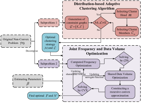
Figure 3: Flow chard of the proposed algorithms.

Without loss of generality, we discuss the computational complexity of the proposed DACA and JFVO algorithms. When addressing the clustering problem, the predominant computational consumption arises from the generation of the constraint graph. The complexity of calculating these constraint edges in DACA is ${\rm O}\left({{K^{2}}}\right)$. For the joint optimization problem, the computational complexity mainly relies on the calculation of the computed frequency, the construction of a recursive convex approximation function, and the solution of the shared data volume. In the outer iteration, the complexity of updating frequency $\boldsymbol{F}$ is ${\rm O}\left({{JK}}\right)$. During the inner iteration, we design a recursive convex approximation for optimizing the shared data volume. The complexity in calculating the surrogate function is ${\rm O}\left({{JIM}}\right)$, where $M$ is the number of the clusters determined by DACA. Additionally, problem (35) is a quadratic problem (QP) [39] and the complexity of solving it using a standard convex optimization method is denoted by ${\rm O}\left({{JIM^{2}}}\right)$.

In summary, besides the advantages of the DACA discussed in Section IV-B, our proposed algorithm can effectively accomplish clustered data sharing and accelerate FEEL training in uncertain environments. Stochastic optimization algorithms can mitigate the instability resulting from parameter estimation. Moreover, the computational requirement of JFVO is affordable, making it suitable for practical use as an online algorithm.

V Simulation and Experimental Results

In this section, we present the results of both numerical simulations and experiments to evaluate the performance of our proposed framework. We employ federated learning for image classification using a circular network area with a radius $r=1,000m$, and the specific parameters used in the simulations are comprehensively enumerated in Table I.

TABLE I: SYSTEM PARAMETERS

Parameter	Value	Parameter	Value
$I$	3 dB	$\gamma_{\text{th}}$	0.005 J
$R$	10	$N_{0}$	-174 dBm/Hz
$P_{\text{BS}}$	1 W	$P_{k}$	0.01 W
$B^{d}$	20 MHz	$f_{\max}$	$1.2\times 10^{3}$ MHz
$B^{u}$	1 MHz	$L_{k}$	$2.5\times 10^{5}$ cycles/sample
$B_{m}^{s}$	1 GHz	$\varsigma$	$4\times 10^{-26}$

V-A Experimental Setup

1) Heterogeneous Data Setting:

Datasets: We evaluate our results using the MNIST [40] and CIFAR-10 datasets [41], which are commonly used image datasets. The MNIST dataset consists of 70,000 grayscale images of handwritten digits from 0 to 9, with each image being a 28x28 pixel square. The dataset is divided into two main sets: a training dataset with 60,000 images and a test dataset with 10,000 images. It is worth noting that each MNIST image consists of 784 pixels, corresponding to $8\times 784$ bits, and a label consisting of 8 bits. Therefore, the total size of each sample is $a=6280$ bits. The CIFAR-10 dataset consists of 10 classes of colored objects with 50,000 training and 10,000 test samples. The local dataset of users are the subsets of the training dataset, and the processing details for these non-IID datasets are as follows:

The label distribution skew: To create disjoint non-IID client training data, partial users receive data partitions from only a single class, while the remaining users select samples without replacement from the training dataset with all labels.

The feature distribution skew is set by the noise-based feature imbalance [12]. The entire dataset is randomly and equally divided among multiple parties. Then all parts add different levels of Gaussian noise to their local datasets to achieve distinct feature distributions.

2) Model Structure: We adopt Convolutional Neural Networks (CNNs) as they are widely used in image classification tasks. For the MNIST dataset, we employ a $2$-layer CNN with two $5\times 5$ convolutional layers and two fully connected layers. During local training, we set the batch size to $10$, the number of epochs $E$ to $1$, and the learning rate $\eta$ to $0.01$ in the SGD optimizer. For the more complex CIFAR-10 dataset, we employ the famous CNN architecture known as VGG-16 [42]. We set the local epoch $E$ to $5$, the local batch size to $50$, and the learning rate $\eta$ to $0.25$. We compare the proposed method to other algorithms on terms of both the accuracy and the communication cost.

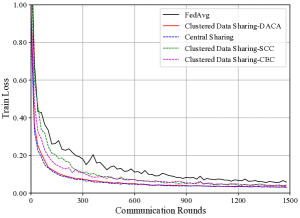
(a) Loss with MNIST data

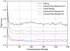
(b) Loss on CIFAR-10 data

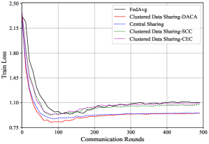
(c) Loss on Feature Distribution Skew

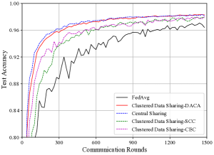
(d) Accuracy on MNIST data

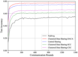
(e) Accuracy on CIFAR-10 data

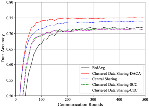
(f) Accuracy on Feature Distribution Skew

Figure 4: The performance compared among baselines and ours, ${v_{th}}=3.5\times 10^{5}$ bit/s and ${e_{th}}=0.5$.

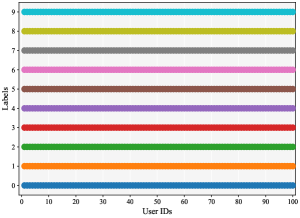
(a) Label distribution of IID data

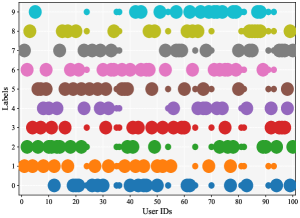
(b) Label distribution before data sharing

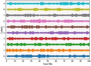
(c) Label distribution after data sharing

Figure 5: The illustration of the number of samples per class allocated to each user (indicated by dot sizes).

Baselines. To demonstrate the performance improvement, the clustered data sharing method is compared with two strategies considering maximized social closeness or data volume.

• FedAvg [4]: Traditional FL with a server and distributed users to train a global model without data sharing.

• FedAvg with Central Sharing [5, 11]: A portion of the global dataset is sent directly by the server to all users.

• Social Closeness Clustering (SCC) [43]: Clustering the users by social closeness, and the most trusted users are selected as cluster heads.

• Communication Efficient Clustering (CEC) [22]: Clustering the users by transmission rate, and the users with high multicast rates are selected as cluster heads.

V-B Experiment Results

1)FL Performance of Clustering Strategies:

In Fig. 4, we compare the proposed DACA with several baselines. Although DACA is primarily designed for label distribution skew, its applicability can be readily extended to other non-IID cases such as feature distribution skew. The left and middle columns of Fig. 4 show the superior performance of the algorithm on different datasets, and the right column shows DACA’s generalization in the performance of feature distribution skew. To ensure fairness, the same shared data volume is used for different clustering strategies. We record the loss values of the local models on their training dataset to show the algorithm convergence, and validate the accuracy of the global model on the test dataset.

From Figs. 4a and 4b, it is evident that the proposed clustered data sharing methods outperform others in terms of reducing the number of communication rounds and achieving lower loss values. Additionally, Figs. 4d and 4e demonstrate that the proposed framework significantly enhances test accuracy. For the MNIST dataset, the accuracy increases from 96.42$\%$ to 98.72$\%$ compared to FedAvg. The CIFAR-10 dataset, being more complex in feature distribution, exhibits even more pronounced improvements, with accuracy rising from 56.14$\%$ to 78.03$\%$ compared to FedAvg. These improvements can be attributed to the fact that the proposed framework reduces the degree of non-IID data and adjusts the deviation of model update by local training. The train loss and test accuracy of DACA are close to central sharing under label distribution skew setting. However, as illustrated in Figs. 4c and 4f, the DACA shows favorable results even compared with central sharing method under feature distribution skew setting. This is because clustered data sharing has a larger sample variety than central sharing, where the former can serve as a better type of data augmentation on local dataset. This observation further demonstrates the superiority of DACA over clustered data sharing in terms of estimating statistical heterogeneity.

It can be observed from Fig. 5a that if the data distribution follows IID distribution, the label distribution across users would be uniform. However, as shown in Fig. 5b, certain users may lack specific labels in non-IID case, leading to distribution skewness. In Fig. 5c, the label distribution after multicasting closely approximates an IID distribution. This is because that our proposed clustered data sharing method effectively addresses skewness by filling missing labels for high EMD users.

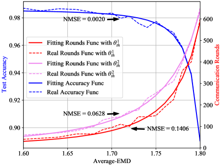
Figure 6: The performance for communication rounds fitting and accuracy fitting. When the accuracy threshold $\theta_{th}^{1}$ is set to 0.95, the estimated parameters are calculated to be ${\beta_{1}=0.50},{\beta_{2}=-1.83},{\beta_{3}=1.70}$. When the accuracy threshold $\theta_{th}^{2}$ is set to 0.96, the estimated parameters are calculated to be ${\beta_{1}=0.24},{\beta_{2}=-0.89},{\beta_{3}=0.06}$.

2) Performance for Data Fitting:

To obtain the communication rounds function $T\left(\cdot\right)$, we conduct a series of FL experiments involving heterogeneous datasets with different average-EMD in Fig. 6. The number of communication rounds is recorded when the test accuracy of the global model first meets the specified threshold. The acquired data from these experiments are used to estimate the fitted parameters $\boldsymbol{\beta}$ in (31). We also record the final accuracy of the global models which are trained on various average-EMD datasets with a sufficient number of rounds. In order to demonstrate the effect of data fitting, the Normal Mean Squared Error (NMSE) serves as an important indicator, which measures the disparities between estimated and actual values. The estimated rounds with smaller NMSE indicate a high-precision fitted parameters $\boldsymbol{\beta}$, which helps complete the proposed optimization algorithm in Figs. 7 and 8.

Fig. 6 effectively demonstrates the performance of the function curve $T\left(\cdot\right)$ under different accuracy thresholds. This figure depicts that the number of communication rounds proportionally increases with the rise in the average EMD of the dataset. The rate of increase remains relatively gradual initially, but escalates as the dataset’s non-IIDness becomes more pronounced. Additionally, as the desired accuracy threshold becomes more demanding, the number of communication rounds correspondingly rises. These observations are consistent with the preliminary experiments in the Section II-C, and highlight a trade-off between maximizing global model accuracy and minimizing communiction rounds. Furthermore, as depicted in this figure, a discernible relationship exists between accuracy and statistical heterogeneity, and this correlation exhibits an inverse trend in comparison to the communication rounds. Consequently, it is crucial to identify an appropriate average-EMD value for balancing the communication cost and model accuracy, i.e., the optimal shared data volume ${{\boldsymbol{N}}^{s}}$.

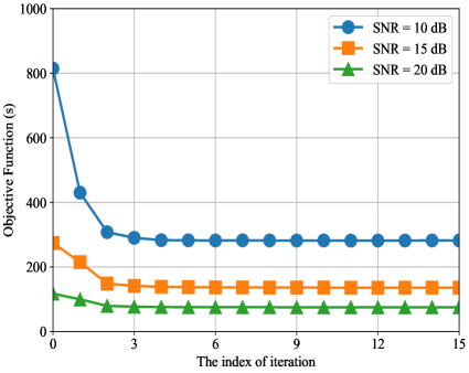
Figure 7: Convergence of the JFVO algorithm.

3) Performance Evaluation of the Optimization Algorithm:

In Fig. 7, the convergence performance of the JFVO algorithm is evaluated at various Signal-Noise-Ratio (SNR). SNR is an important parameter that affects the performance and quality of communication systems. We simulate various communication states by varying the SNR to 10dB, 15dB, and 20dB. This allows us to evaluate the effectiveness of JFVO algorithm in these varied communication states. The depicted results illustrate a consistent decrease in the value of $\Psi$ as the iteration index increases, ultimately converging within a span of 6 iterations. This substantiates the rapid convergence capability of the JFVO algorithm. Moreover, it’s observed that as the SNR increases, the value of $\Psi$ also decreases. This trend is attributed to the reduced delay of clustered data sharing FEEL when users have better channel states in the smaller communication coverage area. A channel with a lower SNR has a higher transmission, which makes the total delay of data sharing and model transmission smaller.

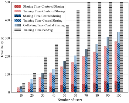
Figure 8: Total delay of federated learning with data sharing.

Fig. 8 illustrates the total delay variation with the number of users. Traditional FL defines FL training delay as total delay, which includes model transmission and local processing. For FedAvg with central sharing, total delay includes data collection, sharing, and FL training. In contrast, clustered data sharing FEEL just considers training and sharing time. In Fig. 8, the total delay of the conventional FedAvg algorithm increases as the number of users grows. This is due to the fact that limited communication resources lead to a reduction in transmission rates and an increase in FL training time. Compared with FedAvg, the total delay of clustered data sharing FEEL can be significantly reduced by employing the DACA and JFOV algorithms. This improvement can be attributed to the optimization of computational resources and a reduction in the number of convergence rounds. Notably, the sharing time gradually increases with the growing number of users. This is because of increased interference among cluster heads, which causes a decrease in the multicast rate of data sharing. Furthermore, the latency of clustered data sharing is slightly lower than that of central sharing, which involves extra delay for data uploading, referred to as Collecting Time.

VI Conclusion

In this work, we investigate and quantify the statistical heterogeneity which is identified as a primary impediment to the convergence of FL. Furthermore, we introduce a clustered data sharing framework to address the non-IID challenge in FEEL and formulate an optimization problem which is aimed at minimize the overall delay in transmission and computation. We decompose the original problem into two subproblem, each dedicated to identifying the optimal clustering strategy and efficient resource allocation. Three conditions are established to aid in clustering process, rooted in a privacy-preserving constrained graph. To enhance the efficacy of data sharing, a clustering algorithm is proposed for selecting cluster heads and credible associates based on the data distribution and the constraints. We derive a upper bound on FEEL convergence to fit the relationship between data distribution and the communication rounds. Then a stochastic optimization approach is employed to determine the optimal computed frequency and shared data volume. The experimental results show that the proposed framework is efficacious in mitigating the data heterogeneity within the system and expediting the FEEL training process. Moreover, our method exhibits well performance not only in resource-constrained environments but also in different non-IID cases.

Appendix A

To prove the contrapositive of Theorem 1: Assume that ${\cal M}^{\prime}$ and ${\cal C}^{\prime}$ (${\cal M}^{\prime}\neq{{\cal M}^{*}}$, ${\cal C}^{\prime}\neq{{\cal C}^{*}}$) not satisfy condition 2, i.e., there exists a cluster member ${c_{0}}\in{{\cal C}^{\prime}_{{m_{0}}}}$ whose ${D_{{\rm{EMD}}}}\left({{c_{0}}}\right)$ is lower than its cluster heads ${m_{0}}\in{\cal M}^{\prime}$. Then we can set ${c_{0}}$ as the cluster head for a new extra cluster, making the ${\tilde{D}_{{\rm{EMD}}}}$ lower. Therefore, ${\cal M}^{\prime}$ and ${\cal C}^{\prime}$ are not the optimal solutions of the problem $\mathcal{P}$. Since ${\cal M}^{\prime}$ and ${\cal C}^{\prime}$ satisfy condition 2 but not satisfy condition 3, the data distributions of the cluster heads are all relatively close to the global distribution. Therefore, the greater the difference in distribution distance between nodes and cluster heads, the greater the shared gain that can be obtained, making ${\tilde{D}_{{\rm{EMD}}}}\left({{\cal M}^{\prime},{\cal C}^{\prime}}\right)>{\tilde{D}_{{\rm{EMD}}}}\left({{{\cal M}^{*}},{{\cal C}^{*}}}\right)$. Hence, ${\cal M}^{\prime}$ and ${\cal C}^{\prime}$ are not the optimal solutions to the problem $\mathcal{P}1^{\prime}$.

Appendix B

VI-A Assumptions and Preliminaries

Assumption 1.

(L-smooth) For all ${w_{1}}$ and ${w_{2}}$, ${F_{k}}\left({{w_{1}}}\right)\leqslant{F_{k}}\left({{w_{2}}}\right)+{\left({{w_{1}}-{w_{2}}}\right)^{T}}\nabla{F_{k}}\left({{w_{2}}}\right)+\frac{L}{2}\left\|{{w_{1}}-{w_{2}}}\right\|_{2}^{2}$.

Assumption 2.

(Convex) For all ${w_{1}}$ and ${w_{2}}$, ${F_{k}}\left({{w_{1}}}\right)\geqslant{F_{k}}\left({{w_{2}}}\right)+{\left({{w_{1}}-{w_{2}}}\right)^{T}}\nabla{F_{k}}\left({{w_{2}}}\right)$.

Assumption 3.

(Unbiasedness and Bounded Variance of local stochastic gradient)

${\mathbb{E}_{\left({x,y}\right)\sim{\mathcal{D}_{k}}}}\left[{\nabla{F_{k}}\left({\left({x,y}\right),w}\right)}\right]=\nabla{F_{k}}\left(w\right)$,

$\mathbb{E}\left[{{{\left\|{\nabla{F_{k}}\left({\left({x,y}\right),{w_{k}}}\right)-\nabla{F_{k}}\left({{w_{k}}}\right)}\right\|}^{2}}}\right]\leqslant{\sigma^{2}}$.

Assumption 4.

(Uniformly Bounded of local stochastic gradients) $\left\|{\nabla{F_{k}}\left({\left({x,y}\right),w}\right)}\right\|\leqslant G$ for all $k=1,...,K$.

At any round $t$, each client $k$ takes $E$ local SGD steps with learning rate $\eta$, i.e., $w_{k}^{\left({t,i+1}\right)}=w_{k}^{\left({t,i}\right)}+\eta\nabla{F_{k}}\big{(}{\left({x,y}\right),w_{k}^{\left({t,i}\right)}}\big{)}$, $\forall i=1,...,E$, $\forall k=1,..,K$. For the sake of simplicity, we set the same ${n_{k}}$ for all clients and the personal heterogeneity as ${D_{k}}=\sum\nolimits_{y}{\left\|{{P_{k}}\left(y\right)-{P_{g}}\left(y\right)}\right\|}$. Then like the works [10, 44], we also use the shadow sequence for clearly analyzing: the virtual global model for each step update ${\bar{w}^{\left({t,i}\right)}}$, and the average EMD $\bar{D}$ can be described as:

$${{\bar{w}^{\left({t,i}\right)}}=\frac{1}{K}\sum\limits_{k}{w_{k}^{\left({t,i}\right)}},\bar{D}=\frac{1}{K}\sum\limits_{k}{{D_{k}}}.}$$

Given this notation, we have

$${{\bar{w}^{\left({t,i+1}\right)}}={\bar{w}^{\left({t,i}\right)}}-\frac{\eta}{K}\sum\limits_{k=1}^{K}{\nabla{F_{k}}\left({\left({x,y}\right),w_{k}^{\left({t,i}\right)}}\right)}.}$$

It is noteworthy that at the end of each round, we have ${\bar{w}^{(t,E)}}={\bar{w}^{\left({t+1,0}\right)}}=w_{k}^{(t+1,0)}$.

VI-B Key Lemmas and Theorem

PROOF SKETCH: First we prove two lemmas, the Lemma 1 gives an upper bound on the convergence of one training round, which shows that the training error of FL comes from two parts, stochastic gradient descent and model drift. Then lemma 2 gives an upper bound on the error of model drift, which is mainly affected by two main factors, the number of local training rounds and the local data distribution (data heterogeneity). Finally we use these two lemmas to derive an upper bound on the FL convergence of the $T$-rounds.

Lemma 1 (Results of one round).

Assuming the client learning rate satisfies $\eta\leqslant\frac{1}{{4L}}$, then

$\begin{gathered}\mathbb{E}\left[{\frac{1}{E}\sum\limits_{i=1}^{E}{F\left({{{\bar{w}}^{\left({t,i}\right)}}}\right)-F\left({{w^{*}}}\right)}}\right]\hfill\\ \leqslant\frac{1}{{2\eta E}}\left({{{\left\|{{{\bar{w}}^{\left({t,0}\right)}}-{w^{*}}}\right\|}^{2}}-\mathbb{E}\left[{{{\left\|{{{\bar{w}}^{\left({t,E}\right)}}-{w^{*}}}\right\|}^{2}}}\right]}\right)\hfill\\ +\underbrace{\frac{{\eta{\sigma^{2}}}}{K}+\frac{L}{{KE}}\sum\limits_{k=1}^{K}{\sum\limits_{i=1}^{E}{\mathbb{E}\left[{{{\left\|{w_{k}^{\left({t,i}\right)}-{{\bar{w}}^{\left({t,i}\right)}}}\right\|}^{2}}}\right]}}.}_{{\color[rgb]{1,0,0}\text{model drift}}}\hfill\\ \end{gathered}$

Remark 1.

Lemma 1 analyzes the convergence bound of a FL round from two terms: the convergence error of stochastic gradient optimization, and the drift between the local model and the virtual global model.

Lemma 2 (Bounded model drift).

Assuming the client learning rate satisfies $\eta\leqslant\frac{1}{{4L}}$, then

$\begin{gathered}\mathbb{E}\left[{{{\left\|{w_{k}^{\left({t,i}\right)}-{{\bar{w}}^{\left({t,i}\right)}}}\right\|}^{2}}}\right]\hfill\\ \leqslant 2{E^{2}}{\eta^{2}}D_{k}^{2}{G^{2}}+6E{\eta^{2}}D_{k}^{2}+4E{\eta^{2}}{\sigma^{2}}.\hfill\\ \end{gathered}$

Remark 2.

Lemma 2 highlights that model drift is influenced by two primary factors: the local step size $E$ and the heterogeneity degree of the local dataset $D_{k}$. The model drift error increases with the larger degree of data heterogeneity. An interesting observation is that model drift error escalates with the growth of the local step size. This phenomenon can be readily understood as increasing the local step size shifts the local models towards the local optimums.

Combine Lemmas 1 and 2 and telescope $t$ from $0$ to $T-1$ to obtain the main theorem as follows:

Theorem 2.

(Convergence rate) Under the aforementioned assumptions (1-4), if the client learning rate satisfies $\eta\leqslant\frac{1}{{4L}}$, then

$\begin{gathered}\mathbb{E}\left[{\frac{1}{{ET}}\sum\limits_{t=0}^{T-1}{\sum\limits_{i=1}^{E}{F\left({{{\bar{w}}^{\left({t,i}\right)}}}\right)-F\left({{w^{*}}}\right)}}}\right]\hfill\\ \leqslant\frac{A}{{2\eta ET}}+\frac{{\eta{\sigma^{2}}}}{K}+2KL{E^{2}}{\eta^{2}}{{\bar{D}}^{2}}{G^{2}}\hfill\\ +6KLE{\eta^{2}}{{\bar{D}}^{2}}+4LE{\eta^{2}}{\sigma^{2}},\end{gathered}$

where $A=\left\|{{w^{\left({0,0}\right)}}-{w^{*}}}\right\|$.

proof: By combining Lemmas 1, and 2, we have

$\begin{gathered}{\mathbb{E}}\left[{\frac{1}{{ET}}\sum\limits_{t=0}^{T-1}{\sum\limits_{i=1}^{E}{F\left({{{\bar{w}}^{\left({t,i}\right)}}}\right)-F\left({{w^{*}}}\right)}}}\right]\end{gathered}$

$\begin{gathered}\leqslant\frac{1}{{2\eta ET}}\sum\limits_{t=0}^{T-1}{\left({{{\left\|{{{\bar{w}}^{\left({t,0}\right)}}-{w^{*}}}\right\|}^{2}}-{\mathbb{E}}\left[{{{\left\|{{{\bar{w}}^{\left({t,E}\right)}}-{w^{*}}}\right\|}^{2}}}\right]}\right)}\hfill\\ \end{gathered}$

$\begin{gathered}+\frac{{\eta{\sigma^{2}}}}{K}+\frac{L}{K}\sum\limits_{k=1}^{K}{\left({2{E^{2}}{\eta^{2}}D_{k}^{2}{G^{2}}+6E{\eta^{2}}D_{k}^{2}+4E{\eta^{2}}{\sigma^{2}}}\right)}\end{gathered}$

$\begin{gathered}\leqslant\frac{1}{{2\eta ET}}{\left\|{{{\bar{w}}^{\left({0,0}\right)}}-{w^{*}}}\right\|^{2}}+\frac{{\eta{\sigma^{2}}}}{K}+4LE{\eta^{2}}{\sigma^{2}}\end{gathered}$

$\begin{gathered}+LK\left({2{E^{2}}{\eta^{2}}{{\left({\sum{\frac{{{D_{k}}}}{K}}}\right)}^{2}}{G^{2}}+6E{\eta^{2}}{{\left({\sum{\frac{{{D_{k}}}}{K}}}\right)}^{2}}}\right)\end{gathered}$

$\begin{gathered}\leqslant\frac{A}{{2\eta ET}}+\frac{{\eta{\sigma^{2}}}}{K}+2LK{E^{2}}{\eta^{2}}{{\bar{D}}^{2}}{G^{2}}\end{gathered}$

$\begin{gathered}+6LKE{\eta^{2}}{{\bar{D}}^{2}}+4LE{\eta^{2}}{\sigma^{2}}.\end{gathered}$

Remark 3.

Theorem 2 shows that to attain a fixed precision $\theta$, the number of communications is $\small{T_{\theta}\!=\!{\rm O}\left({\frac{1}{{\beta-{D^{2}}}}}\right)}$, Here $\beta$ is a constant for normalization. We have another insight that the convergence rate is not continue increase as the number of users $K$ increase. Although increasing $K$ can reduce the variance due to the stochastic gradients, it also increase the error from the model drift (Lemma 2).

VI-C The proof of the Lemmas

Proof of Lemma 1:

$\begin{gathered}F\left({{{\bar{w}}^{\left({t,i}\right)}}}\right)-F\left({{w^{*}}}\right)=\frac{1}{K}\sum\limits_{k=1}^{K}{\left({{F_{k}}\left({{{\bar{w}}^{\left({t,i}\right)}}}\right)-F\left({{w^{*}}}\right)}\right)}\end{gathered}$

$\begin{gathered}=\frac{1}{K}\sum\limits_{k=1}^{K}{\left({{F_{k}}\left({{{\bar{w}}^{\left({t,i}\right)}}}\right)-{F_{k}}\left({w_{k}^{\left({t,i-1}\right)}}\right)}\right.}\end{gathered}$

$\begin{gathered}\left.{+{F_{k}}\left({w_{k}^{\left({t,i-1}\right)}}\right)-F\left({{w^{*}}}\right)}\right)\end{gathered}$

$\begin{gathered}\mathop{\leqslant}\limits^{a}\frac{1}{K}\sum\limits_{k=1}^{K}{\left[{\left\langle{\nabla{F_{k}}\left({w_{k}^{\left({t,i-1}\right)}}\right),{{\bar{w}}^{\left({t,i}\right)}}-w_{k}^{\left({t.i-1}\right)}}\right\rangle}\right.}\end{gathered}$

$\begin{gathered}+\frac{L}{2}{\left\|{{{\bar{w}}^{\left({t,i}\right)}}\!-\!w_{k}^{\left({t.i-1}\right)}}\right\|^{2}}\left.{\!-\!\left(\!{{w^{*}}\!-\!w_{k}^{\left(\!{t.i\!-\!1}\right)}}\!\right)\nabla{F_{k}}\left({w_{k}^{\left({t,i\!-\!1}\right)}}\right)}\right]\end{gathered}$

$\begin{gathered}=\frac{1}{K}\sum\limits_{k=1}^{K}{\left[{\left\langle{\nabla{F_{k}}\left({w_{k}^{\left({t,i-1}\right)}}\right),{{\bar{w}}^{\left({t,i}\right)}}-{w^{*}}}\right\rangle}\right.}\end{gathered}$

$\begin{gathered}\left.{+\frac{L}{2}{{\left\|{{{\bar{w}}^{\left({t,i}\right)}}-w_{k}^{\left({t.i-1}\right)}}\right\|}^{2}}}\right]\end{gathered}$

$\begin{gathered}\mathop{\leqslant}\limits^{b}\frac{1}{K}\sum\limits_{k=1}^{K}{\left\langle{\nabla{F_{k}}\left({w_{k}^{\left({t,i-1}\right)}}\right),{{\bar{w}}^{\left({t,i}\right)}}-{w^{*}}}\right\rangle}\end{gathered}$

$$\small{\begin{gathered}+L{\left\|{{{\bar{w}}^{\left({t,i}\right)}}\!-\!{{\bar{w}}^{\left({t,i-1}\right)}}}\right\|^{2}}+\frac{L}{K}\sum\limits_{k=1}^{K}{{{\left\|{{{\bar{w}}^{\left({t,i-1}\right)}}\!-\!w_{k}^{\left({t.i-1}\right)}}\right\|}^{2}}},\;\;\end{gathered}}$$ (37)

where the former part of (a) is obtained from Assumption 1 and the latter part is obtained from Assumption 2, and (b) results from the equation ${\left\|{A\!+\!B}\right\|^{2}}\!\leqslant\!2{\left\|A\right\|^{2}}\!+\!2{\left\|B\right\|^{2}}$, where $A={\bar{w}^{\left({t,i}\right)}}-{\bar{w}^{\left({t,i-1}\right)}}$ and $B={\bar{w}^{\left({t,i-1}\right)}}-\bar{w}_{k}^{\left({t,i-1}\right)}$.

$\begin{gathered}\mathbb{E}\left[\frac{1}{K}\sum_{k=1}^{K}\langle\nabla F_{k}(w_{k}^{(t,i-1)}),\bar{w}^{(t,i)}-w^{*}\rangle\right]\end{gathered}$

$\begin{gathered}=\mathbb{E}\left[\frac{1}{K}\!\sum_{k=1}^{K}\langle\!\nabla\!F_{k}(w_{k}^{(t,\!i\!-\!1\!)})\!-\!\nabla F_{k}((x,y),w_{k}^{(t,\!i\!-\!1\!)}),\bar{w}^{(t,i)}\!-\!w^{*}\rangle\right]\end{gathered}$

$\begin{gathered}+\mathbb{E}\left[\frac{1}{K}\sum_{k=1}^{K}\langle\nabla F_{k}((x,y),w_{k}^{(t,i-1)}),\bar{w}^{(t,i)}-w^{*}\rangle\right]\end{gathered}$

$\begin{gathered}\mathop{=}\limits^{(a)}\!\mathbb{E}\!\left[\!\frac{1}{K}\!\sum_{k=1}^{K}\!\langle\nabla\!F_{k}(w_{k}^{(t,i-1)}\!)\!-\!\nabla\!F_{k}(\!(x,y),\!w_{k}^{(t,\!i\!-\!1\!)}\!),\!\bar{w}^{(t,\!i)}\!-\!\bar{w}^{(t,\!i\!-\!1\!)}\!\rangle\!\right]\end{gathered}$

$\begin{gathered}+\mathbb{E}\left[\frac{1}{\eta}\langle\bar{w}^{(t,i-1)}-\bar{w}^{(t,i)},\bar{w}^{(t,i)}-w^{*}\rangle\right]\end{gathered}$

$\begin{gathered}\mathop{\leqslant}\limits^{(b)}\!\eta\mathbb{E}\left[\left\|\frac{1}{K}\sum_{k=1}^{K}\!\left(\!\nabla\!F_{k}(w_{k}^{(t,\!i\!-\!1\!)})\!-\!\nabla F_{k}((x,y),w_{k}^{(t,\!i\!-\!1\!)})\right)\!\right\|^{2}\!\right]\end{gathered}$

$\begin{gathered}+\frac{1}{4\eta}\left\|\bar{w}^{(t,i)}-\bar{w}^{(t,i-1)}\right\|^{2}\end{gathered}$

$\begin{gathered}+\frac{1}{2\eta}\!\left(\!\left\|\bar{w}^{(t,i-1)}\!-\!w^{*}\right\|^{2}\!-\!\left\|\bar{w}^{(t,i-1)}\!-\!\bar{w}^{(t,i)}\right\|^{2}\!-\!\left\|\bar{w}^{(t,i)}\!-\!w^{*}\right\|^{2}\right)\end{gathered}$

$\begin{gathered}\leqslant\frac{\eta\sigma^{2}}{K}-\frac{1}{4\eta}\left\|\bar{w}^{(t,i)}-\bar{w}^{(t,i-1)}\right\|^{2}\end{gathered}$

$$\;\;\;+\frac{1}{2\eta}\left(\left\|\bar{w}^{(t,i-1)}-w^{*}\right\|^{2}-\left\|\bar{w}^{(t,i)}-w^{*}\right\|^{2}\right),$$ (38)

where the former part of (a) holds due to $\mathbb{E}\left[{\nabla{F_{k}}\left({\left({x,y}\right),w}\right)-\nabla{F_{k}}\left(\!w\!\right)}\right]=0$, and the latter part results from perfect square trinomial $2\left\langle{a,b}\right\rangle\!=\!{\left\|{a\!+\!b}\right\|^{2}}\!-\!{\left\|a\right\|^{2}}\!-\!{\left\|b\right\|^{2}}$.

Recalling the (37) and plugging (38) into it, we have $\begin{gathered}\mathbb{E}\left({F\left({{{\bar{w}}^{\left({t,i}\right)}}}\right)-F\left({{w^{*}}}\right)}\right)\end{gathered}$

$\begin{gathered}\leqslant\frac{{\eta{\sigma^{2}}}}{K}\!-\!\left(\!{\frac{1}{{4\eta}}\!-\!L}\!\right)\!{\left\|{{{\bar{w}}^{\left(\!{t,i}\right)}}\!-\!{{\bar{w}}^{\left(\!{t,\!i\!-\!1}\!\right)}}}\right\|^{2}}\!+\!\frac{L}{K}\sum\limits_{k=1}^{K}{{{\!\left\|{{{\bar{w}}^{\left({t,i\!-\!1}\right)}}-w_{k}^{\left(\!{t,\!i\!-\!1}\!\right)}}\right\|}^{2}}}\end{gathered}$

$\begin{gathered}+\frac{1}{{2\eta}}\left({{{\left\|{{{\bar{w}}^{\left({t,i-1}\right)}}-{w^{*}}}\right\|}^{2}}-{{\left\|{{{\bar{w}}^{\left({t,i}\right)}}-{w^{*}}}\right\|}^{2}}}\right)\end{gathered}$

$\begin{gathered}\mathop{\leqslant}\limits^{(a)}\frac{{\eta{\sigma^{2}}}}{K}+\frac{L}{K}\sum\limits_{k=1}^{K}{{{\left\|{{{\bar{w}}^{\left({t,i-1}\right)}}-w_{k}^{\left({t.i-1}\right)}}\right\|}^{2}}}\end{gathered}$

$$+\frac{1}{2\eta}\left(\left\|{\bar{w}^{(t,i-1)}-w^{*}}\right\|^{2}-\left\|{\bar{w}^{(t,i)}-w^{*}}\right\|^{2}\right),$$ (39)

where the client learning rate satisfies $\eta\leqslant\frac{1}{{4L}}$. Telescoping $i$ from $0$ to $E$ completes the proof of Lemma 1.

Proof of Lemma 2:

$\begin{gathered}\left\|{\nabla{F_{k}}\left(w\right)-\nabla F\left(w\right)}\right\|\end{gathered}$

$\begin{gathered}=\left\|{{\mathbb{E}_{\left({x,y}\right)\sim{{\mathcal{P}}_{k}}}}\left[{\nabla F\left({x,y,w}\right)}\right]}\right.\hfill\\ \left.{-{\mathbb{E}_{\left({x,y}\right)\sim{{\mathcal{P}}_{g}}}}\left[{\nabla F\left({x,y,w}\right)}\right]}\right\|\end{gathered}$

$\begin{gathered}=\left\|{\scalebox{1.0}{$\iint$}{{P_{k}}\left({x,y}\right)\nabla F\left({x,y,w}\right)}dxdy}\right.\end{gathered}$

$\begin{gathered}\left.{-\scalebox{1.0}{$\iint$}{{P_{g}}\left({x,y}\right)\nabla F\left({x,y,w}\right)}dxdy}\right\|\end{gathered}$

$\begin{gathered}\leqslant\scalebox{1.0}{$\iint$}{\left\|{\left({{P_{k}}\left({x,y}\right)-{P_{g}}\left({x,y}\right)}\right)\nabla F\left({x,y,w}\right)}\right\|}dxdy\end{gathered}$

$\begin{gathered}\leqslant\scalebox{1.0}{$\int_{y}$}{\left\|{{P_{k}}\left(y\right)-{P_{g}}\left(y\right)}\right\|}\end{gathered}$

$\begin{gathered}\scalebox{1.0}{$\int_{x}$}{\left\|{{P_{k}}\left({\left.x\right|y}\right)\nabla F\left({x,y,w}\right)}\right\|}dxdy\end{gathered}$

$\begin{gathered}=\scalebox{1.0}{$\int_{y}$}{\left\|{{P_{k}}\left(y\right)-{P_{g}}\left(y\right)}\right\|}\end{gathered}$

$\begin{gathered}\left(\scalebox{1.0}{$\int_{x}$}{\left\|{{P_{k}}\left({\left.x\right|y}\right)\nabla F\left({x,y,w}\right)}\right\|}dx\right)dy\end{gathered}$

$\begin{gathered}=\sum\limits_{y=1}^{Y}{\left\|{{P_{k}}\left(y\right)-{P_{g}}\left(y\right)}\right\|{\mathbb{E}_{\left.x\right|y}}\left[{\left\|{\nabla F\left({x,y,w}\right)}\right\|}\right]}\end{gathered}$

$$\,\,\,\,\leqslant{D_{k}}G.$$ (40)

This inequality can be applied to other non-iid cases as well, simply by replacing the distribution function, i.e., ${P_{k}}\left(y\right)$.

$\begin{gathered}{\mathbb{E}}\left[{{{\left\|{w_{1}^{\left({t,i+1}\right)}-w_{2}^{\left({t,i+1}\right)}}\right\|}^{2}}}\right]\end{gathered}$

$\begin{gathered}={\mathbb{E}}\left[{\left\|{w_{1}^{\left({t,i}\right)}-w_{2}^{\left({t,i}\right)}}\right.}\right.\end{gathered}$

$\begin{gathered}\left.{-{{\left.{\eta\left({\nabla{F_{1}}\left({\left({x,y}\right),w_{1}^{\left({t,i}\right)}}\right)-\nabla{F_{2}}\left({\left({x,y}\right),w_{2}^{\left({t,i}\right)}}\right)}\right)}\right\|}^{2}}}\right]\end{gathered}$

$\begin{gathered}\leqslant{\mathbb{E}}\left[{{{\left\|{w_{1}^{\left({t,i}\right)}-w_{2}^{\left({t,i}\right)}}\right\|}^{2}}}\right.\end{gathered}$

$\begin{gathered}-2\eta\!\left\langle\!{\nabla{F_{1}}\!\left({\left(\!{x,y}\!\right),\!w_{1}^{\left(\!{t,i}\!\right)}}\!\right)\!-\!\nabla{F_{2}}\left(\!{\left(\!{x,y}\right),\!w_{2}^{\left({t,i}\!\right)}}\right)}\!\right.,\left.{w_{1}^{\left({t,i}\right)}\!-\!w_{2}^{\left(\!{t,i}\!\right)}}\right\rangle\end{gathered}$

$\begin{gathered}\left.{+{\eta^{2}}{{\left\|{\nabla{F_{1}}\left({\left({x,y}\right),w_{1}^{\left({t,i}\right)}}\right)-\nabla{F_{2}}\left({\left({x,y}\right),w_{2}^{\left({t,i}\right)}}\right)}\right\|}^{2}}}\right]\end{gathered}$

$\begin{gathered}\left.{+{\eta^{2}}{{\left\|{\nabla{F_{1}}\left({\left({x,y}\right),w_{1}^{\left({t,i}\right)}}\right)-\nabla{F_{2}}\left({\left({x,y}\right),w_{2}^{\left({t,i}\right)}}\right)}\right\|}^{2}}}\right]\end{gathered}$

$\begin{gathered}-2\eta\left\langle{\nabla{F_{1}}\left({w_{1}^{\left({t,i}\right)}}\right)}\right.-\nabla{F_{2}}\left({w_{2}^{\left({t,i}\right)}}\right),\left.{w_{1}^{\left({t,i}\right)}-w_{2}^{\left({t,i}\right)}}\right\rangle\end{gathered}$

$\begin{gathered}+{\eta^{2}}\left\|{\left({\nabla{F_{1}}\left({\left({x,y}\right),w_{1}^{\left({t,i}\right)}}\right)-\nabla{F_{1}}\left({w_{1}^{\left({t,i}\right)}}\right)}\right)}\right.\end{gathered}$

$\begin{gathered}-\left({\nabla{F_{2}}\left({\left({x,y}\right),w_{2}^{\left({t,i}\right)}}\right)-\nabla{F_{2}}\left({w_{2}^{\left({t,i}\right)}}\right)}\right)\end{gathered}$

$\begin{gathered}+{\left.{\left({\nabla{F_{1}}\left({w_{1}^{\left({t,i}\right)}}\right)-\nabla{F_{2}}\left({w_{2}^{\left({t,i}\right)}}\right)}\right)}\right\|^{2}}\end{gathered}$

$\begin{gathered}\mathop{\leqslant}\limits^{a}{\left\|{w_{1}^{\left({t,i}\right)}-w_{2}^{\left({t,i}\right)}}\right\|^{2}}\end{gathered}$

$\begin{gathered}-2\eta\underbrace{\left\langle{\nabla{F_{1}}\left({w_{1}^{\left({t,i}\right)}}\right)}\right.-\nabla{F_{2}}\left({w_{2}^{\left({t,i}\right)}}\right),\left.{w_{1}^{\left({t,i}\right)}-w_{2}^{\left({t,i}\right)}}\right\rangle}_{{\color[rgb]{1,0,0}\text{B}}}\end{gathered}$

$${\small{\begin{gathered}+{\eta^{2}}{\underbrace{{\left\|{\nabla{F_{1}}\left({w_{1}^{\left({t,i}\right)}}\right)-\nabla{F_{2}}\left({w_{2}^{\left({t,i}\right)}}\right)}\right\|}^{2}}_{{\color[rgb]{1,0,0}\text{C}}}}+2{\eta^{2}}{\sigma^{2}}.\quad\quad\quad\hfill\\ \end{gathered}}}$$ (41)

We next focus on bounding $B$ and $C$:

$\begin{gathered}-B=-\left\langle{\nabla{F_{1}}\left({w_{1}^{\left({t,i}\right)}}\right)}\right.-\nabla{F_{2}}\left({w_{2}^{\left({t,i}\right)}}\right),\left.{w_{1}^{\left({t,i}\right)}-w_{2}^{\left({t,i}\right)}}\right\rangle\end{gathered}$

$\begin{gathered}\leqslant-\left\langle{\nabla F\left({w_{1}^{\left({t,i}\right)}}\right)}\right.-\nabla F\left({w_{2}^{\left({t,i}\right)}}\right),\left.{w_{1}^{\left({t,i}\right)}-w_{2}^{\left({t,i}\right)}}\right\rangle\end{gathered}$

$\begin{gathered}+\left\langle{\nabla F\left({w_{1}^{\left({t,i}\right)}}\right)}\right.-\nabla{F_{1}}\left({w_{1}^{\left({t,i}\right)}}\right),\left.{w_{1}^{\left({t,i}\right)}-w_{2}^{\left({t,i}\right)}}\right\rangle\end{gathered}$

$\begin{gathered}+\left\langle{\nabla{F_{2}}\left({w_{2}^{\left({t,i}\right)}}\right)}\right.-\nabla F\left({w_{2}^{\left({t,i}\right)}}\right),\left.{w_{1}^{\left({t,i}\right)}-w_{2}^{\left({t,i}\right)}}\right\rangle\end{gathered}$

$\begin{gathered}\mathop{\leqslant}\limits^{a}\frac{{-1}}{L}{\left\|{\nabla F\left({w_{1}^{\left({t,i}\right)}}\right)-\nabla F\left({w_{2}^{\left({t,i}\right)}}\right)}\right\|^{2}}\end{gathered}$

$\begin{gathered}+\left({{D_{1}}+{D_{2}}}\right)G\left\|{w_{1}^{\left({t,i}\right)}-w_{2}^{\left({t,i}\right)}}\right\|\end{gathered}$

$\begin{gathered}\leqslant\frac{{-1}}{L}{\left\|{\nabla F\left({w_{1}^{\left({t,i}\right)}}\right)-\nabla F\left({w_{2}^{\left({t,i}\right)}}\right)}\right\|^{2}}\end{gathered}$

$${\small{\begin{gathered}+\frac{1}{{2\eta E}}{\left\|{w_{1}^{\left({t,i}\right)}-w_{2}^{\left({t,i}\right)}}\right\|^{2}}+2\eta E\left({{D_{1}}+{D_{2}}}\right)G,\quad\quad\quad\quad\hfill\\ \end{gathered}}}$$ (42)

where the former term of inequality $(a)$ can be can be derived based on Assumptions 1 and 2, and the second term is based on (40). Similarly, the $C$ is bounded as:

$${\small{\begin{gathered}C={\left\|{\nabla{F_{1}}\left({w_{1}^{\left({t,i}\right)}}\right)-\nabla{F_{2}}\left({w_{2}^{\left({t,i}\right)}}\right)}\right\|^{2}}\hfill\\ \leqslant\left\|{\left({\nabla F\left({w_{1}^{\left({t,i}\right)}}\right)-\nabla F\left({w_{2}^{\left({t,i}\right)}}\right)}\right)}\right.+\left({\nabla{F_{1}}\left({w_{1}^{\left({t,i}\right)}}\right)}\right.\hfill\\ -\left.{\nabla F\left({w_{1}^{\left({t,i}\right)}}\right)}\right){\left.{+\left({\nabla F\left({w_{2}^{\left({t,i}\right)}}\right)-\nabla{F_{2}}\left({w_{2}^{\left({t,i}\right)}}\right)}\right)}\right\|^{2}}\hfill\\ \leqslant 3{\left\|{\nabla F\left({w_{1}^{\left({t,i}\right)}}\right)-\nabla F\left({w_{2}^{\left({t,i}\right)}}\right)}\right\|^{2}}+3D_{1}^{2}+3D_{2}^{2}.\hfill\\ \end{gathered}}}$$ (43)

Replacing the bounds (42) and (43) back to the (41), we have

$${\small{\begin{gathered}{\mathbb{E}}\left[{{{\left\|{w_{1}^{\left({t,i+1}\right)}-w_{2}^{\left({t,i+1}\right)}}\right\|}^{2}}}\right]\hfill\\ \leqslant\left({1+\frac{1}{E}}\right){\left\|{w_{1}^{\left({t,i}\right)}-w_{2}^{\left({t,i}\right)}}\right\|^{2}}\hfill\\ -\left({\frac{{2\eta}}{L}-3{\eta^{2}}}\right)\left({\nabla F\left({w_{1}^{\left({t,i}\right)}}\right)-\nabla F\left({w_{2}^{\left({t,i}\right)}}\right)}\right)\hfill\\ +E{\eta^{2}}{G^{2}}{\left({{D_{1}}+{D_{2}}}\right)^{2}}+3{\eta^{2}}D_{1}^{2}+3{\eta^{2}}D_{2}^{2}+2{\eta^{2}}{\sigma^{2}}\hfill\\ \mathop{\leqslant}\limits^{a}\left({1+\frac{1}{E}}\right){\left\|{w_{1}^{\left({t,i}\right)}-w_{2}^{\left({t,i}\right)}}\right\|^{2}}\hfill\\ +E{\eta^{2}}{G^{2}}{\left({{D_{1}}+{D_{2}}}\right)^{2}}+3{\eta^{2}}D_{1}^{2}+3{\eta^{2}}D_{2}^{2}+2{\eta^{2}}{\sigma^{2}},\hfill\\ \end{gathered}}}$$ (44)

where (a) holds due to $\eta\leqslant\frac{1}{{4L}}$. Then it can be derived by conducting a geometric series:

$${\small{\begin{gathered}{\mathbb{E}}\left[{{{\left\|{w_{1}^{\left({t,i}\right)}-w_{2}^{\left({t,i}\right)}}\right\|}^{2}}}\right]\hfill\\ \leqslant\frac{{{{\left({1\!+\!\frac{1}{E}}\right)}^{i}}\!-\!1}}{{{1\mathord{\left/{\vphantom{1E}}\right.\kern-1.2pt}E}}}\!\left[{E{\eta^{2}}{G^{2}}{{\left({{D_{1}}\!+\!{D_{2}}}\right)}^{2}}\!+\!3{\eta^{2}}D_{1}^{2}\!+\!3{\eta^{2}}D_{2}^{2}\!+\!2{\eta^{2}}{\sigma^{2}}}\right]\hfill\\ \leqslant 2{E^{2}}{\eta^{2}}{G^{2}}{\left({{D_{1}}+{D_{2}}}\right)^{2}}+6E{\eta^{2}}D_{1}^{2}+6E{\eta^{2}}D_{2}^{2}+4E{\eta^{2}}{\sigma^{2}}.\hfill\\ \end{gathered}}}$$ (45)

Replacing $w_{1}^{\left({t,i}\right)}$ as $w_{k}^{\left({t,i}\right)}$, and $w_{2}^{\left({t,i}\right)}$ as ${{\bar{w}}^{\left({t,i}\right)}}$, we have

$\begin{gathered}\mathbb{E}\left[{{{\left\|{w_{k}^{\left({t,i}\right)}-{{\bar{w}}^{\left({t,i}\right)}}}\right\|}^{2}}}\right]\hfill\\ \leqslant 2{E^{2}}{\eta^{2}}{G^{2}}D_{k}^{2}+6E{\eta^{2}}D_{k}^{2}+4E{\eta^{2}}{\sigma^{2}},\hfill\\ \end{gathered}$

and the proof is completed.

References

- [1] G. Hu, Y. Teng, N. Wang, and F. R. Yu, “Clustered data sharing for non-iid federated learning over wireless networks,” in Proc. IEEE Int. Conf. Commun. (ICC), Rome, Italy, May 2023, pp. 1175–1180.
- [2] W. Y. B. Lim, N. C. Luong, D. T. Hoang, Y. Jiao, Y.-C. Liang, Q. Yang, D. Niyato, and C. Miao, “Federated learning in mobile edge networks: A comprehensive survey,” IEEE Commun. Surv. Tutor., vol. 22, no. 3, pp. 2031–2063, Thirdquarter 2020.
- [3] C. Tikkinen-Piri, A. Rohunen, and J. Markkula, EU General Data Protection Regulation: Changes and implications for personal data collecting companies, Feb. 2018, vol. 34, no. 1.
- [4] B. McMahan, E. Moore, D. Ramage, S. Hampson, and B. A. y Arcas, “Communication-efficient learning of deep networks from decentralized data,” in Proc. 20th Int. Conf. Artif. Intell. Stat. (AISTATS), Fort Lauderdale, FL, Apr. 2017, pp. 1273–1282.
- [5] Y. Zhao, M. Li, L. Lai, N. Suda, D. Civin, and V. Chandra, “Federated learning with non-iid data,” arXiv preprint arXiv:1806.00582, Jun. 2018.
- [6] P. Kairouz, H. B. McMahan, B. Avent, A. Bellet, M. Bennis, A. N. Bhagoji, K. Bonawitz, Z. Charles, G. Cormode, R. Cummings et al., “Advances and open problems in federated learning,” Found. Trends Mach. Learn., vol. 14, no. 1–2, pp. 1–210, Jun. 2021.
- [7] A. J. Thirunavukarasu, D. S. J. Ting, K. Elangovan, L. Gutierrez, T. F. Tan, and D. S. W. Ting, “Large language models in medicine,” Nat. Med., vol. 29, no. 8, pp. 1930–1940, Aug. 2023.
- [8] R. Yu and P. Li, “Toward resource-efficient federated learning in mobile edge computing,” IEEE Netw., vol. 35, no. 1, pp. 148–155, Jan./Feb. 2021.
- [9] H. Wang, Z. Kaplan, D. Niu, and B. Li, “Optimizing federated learning on non-iid data with reinforcement learning,” in Proc. IEEE Conf. Comput. Commun (INFOCOM), Toronto, ON, Canada, Jul. 2020, pp. 1698–1707.
- [10] X. Li, K. Huang, W. Yang, S. Wang, and Z. Zhang, “On the convergence of fedavg on non-iid data,” in Proc. Int. Conf. Learn. Represent. (ICLR), Addis Ababa, Ethiopia, Apr. 2020.
- [11] Z. Zhao, C. Feng, W. Hong, J. Jiang, C. Jia, T. Q. Quek, and M. Peng, “Federated learning with non-iid data in wireless networks,” IEEE Trans. Wirel. Commun., vol. 21, no. 3, pp. 1927–1942, Sep. 2021.
- [12] Q. Li, Y. Diao, Q. Chen, and B. He, “Federated learning on non-iid data silos: An experimental study,” in Proc. Int. Conf. Data. Eng. (ICDE), Virtual-Online, May 2022, pp. 965–978.
- [13] M. Ye, X. Fang, B. Du, P. C. Yuen, and D. Tao, “Heterogeneous federated learning: State-of-the-art and research challenges,” ACM Comput. Surv., vol. 56, no. 3, pp. 1–44, Oct. 2023.
- [14] T. Li, A. K. Sahu, M. Zaheer, M. Sanjabi, A. Talwalkar, and V. Smith, “Federated optimization in heterogeneous networks,” Proc. Mach. Learn. Syst. (MLSys), vol. 2, no. 1, pp. 429–450, Mar. 2020.
- [15] J. Wang, Q. Liu, H. Liang, G. Joshi, and H. V. Poor, “Tackling the objective inconsistency problem in heterogeneous federated optimization,” in Adv. Neural Inf. Process. Syst. (NeurIPS), vol. 33, Virtual-Online, Dec. 2020, pp. 7611–7623.
- [16] S. P. Karimireddy, S. Kale, M. Mohri, S. Reddi, S. Stich, and A. T. Suresh, “Scaffold: Stochastic controlled averaging for federated learning,” in Proc. Int. Conf. Mach. Learn. (ICML), Virtual-Online, Jul. 2020, pp. 5132–5143.
- [17] A. Ghosh, J. Chung, D. Yin, and K. Ramchandran, “An efficient framework for clustered federated learning,” IEEE Trans. Inf. Theory, vol. 68, no. 12, pp. 8076 – 8091, Dec. 2022.
- [18] F. Sattler, K.-R. Müller, and W. Samek, “Clustered federated learning: Model-agnostic distributed multitask optimization under privacy constraints,” IEEE Trans. Neural Netw. Learn. Syst., vol. 32, no. 8, pp. 3710–3722, Aug. 2021.
- [19] C. Chen, Z. Chen, Y. Zhou, and B. Kailkhura, “Fedcluster: Boosting the convergence of federated learning via cluster-cycling,” in Proc. - IEEE Int. Conf. Big Data (Big Data), Virtual-Online, Dec. 2020, pp. 5017–5026.
- [20] Z. Zhu, J. Hong, and J. Zhou, “Data-free knowledge distillation for heterogeneous federated learning,” in Proc. Int. Conf. Mach. Learn. (ICML), Virtual-Online, Jul. 2021, pp. 12 878–12 889.
- [21] D. Li and J. Wang, “Fedmd: Heterogenous federated learning via model distillation,” Vancouver, BC, Canada, Sep. 2019.
- [22] X. Cai, X. Mo, J. Chen, and J. Xu, “D2d-enabled data sharing for distributed machine learning at wireless network edge,” IEEE Wirel. Commun. Lett., vol. 9, no. 9, pp. 1457–1461, Sep. 2020.
- [23] N. Yoshida, T. Nishio, M. Morikura, K. Yamamoto, and R. Yonetani, “Hybrid-fl for wireless networks: Cooperative learning mechanism using non-iid data,” in Proc. IEEE Int. Conf. Commun. (ICC), Dublin, Ireland, Jun. 2020.
- [24] H. Gu, B. Guo, J. Wang, W. Sun, J. Liu, S. Liu, and Z. Yu, “Fedaux: An efficient framework for hybrid federated learning,” in Int. Conf. Commun. (ICC), Seoul, Korea, Republic of, May 2022, pp. 195–200.
- [25] M. Chen, Z. Yang, W. Saad, C. Yin, H. V. Poor, and S. Cui, “A joint learning and communications framework for federated learning over wireless networks,” IEEE Trans. Wirel. Commun., vol. 20, no. 1, pp. 269–283, Jan. 2020.
- [26] E. Seo, D. Niyato, and E. Elmroth, “Resource-efficient federated learning with non-iid data: An auction theoretic approach,” IEEE Internet Things J., vol. 9, no. 24, pp. 25 506–25 524, Dec. 2022.
- [27] N. Chukhno, O. Chukhno, D. Moltchanov, S. Pizzi, A. Gaydamaka, A. Samuylov, A. Molinaro, Y. Koucheryavy, A. Iera, and G. Araniti, “Models, methods, and solutions for multicasting in 5g/6g mmwave and sub-thz systems,” IEEE Commun. Surv. Tutor., vol. 26, no. 1, pp. 119–159, Firstquarter 2024.
- [28] N. Chukhno, O. Chukhno, S. Pizzi, A. Molinaro, A. Iera, and G. Araniti, “Beyond complexity limits: Machine learning for sidelink-assisted mmwave multicasting in 6g,” IEEE Trans. Broadcast. early access, pp. 1–15, Apr. 2024, doi: 10.1109/TBC.2024.3382959.
- [29] J. Lee, H. Ko, S. Seo, and S. Pack, “Data distribution-aware online client selection algorithm for federated learning in heterogeneous networks,” IEEE Trans. Veh. Technol., vol. 72, no. 1, pp. 1127–1136, Jan. 2022.
- [30] X. Zhang, H. Gu, L. Fan, K. Chen, and Q. Yang, “No free lunch theorem for security and utility in federated learning,” ACM Trans. Intell. Syst. Technol., vol. 14, no. 1, pp. 1–35, Nov. 2022.
- [31] J. Kang, Z. Xiong, D. Niyato, S. Xie, and J. Zhang, “Incentive mechanism for reliable federated learning: A joint optimization approach to combining reputation and contract theory,” IEEE Internet Things J., vol. 6, no. 6, pp. 10 700–10 714, Dec. 2019.
- [32] Z. Su, Y. Wang, T. H. Luan, N. Zhang, F. Li, T. Chen, and H. Cao, “Secure and efficient federated learning for smart grid with edge-cloud collaboration,” IEEE Trans. Ind. Inform., vol. 18, no. 2, pp. 1333–1344, Feb. 2022.
- [33] L. Bottou, “Large-scale machine learning with stochastic gradient descent,” in Int. Conf. Comput. Stat., , Keynote, Invited and Contrib. Pap. (COMPSTAT), Heidelberg, Germany, Sep. 2010, pp. 177–186.
- [34] Y. Li, T. Wu, P. Hui, D. Jin, and S. Chen, “Social-aware d2d communications: qualitative insights and quantitative analysis,” IEEE Commun. Mag., vol. 52, no. 6, pp. 150–158, Jun. 2014.
- [35] G. Zhang, K. Yang, and H.-H. Chen, “Socially aware cluster formation and radio resource allocation in d2d networks,” IEEE Trans. Wirel. Commun., vol. 23, no. 4, pp. 68–73, Aug. 2016.
- [36] “Study on channel model for frequencies from 0.5 to 100 ghz; (release14), version 14.1.1,” 3GPP, Sophia Antipolis, France, Tech. Rep. TR 25.913 V7.3.0 (2006-03), Jul. 2017.
- [37] Q. Zeng, Y. Du, K. Huang, and K. K. Leung, “Energy-efficient radio resource allocation for federated edge learning,” in IEEE Int. Conf. Commun. Workshops (ICC Workshops), Dublin, Ireland, Jun. 2020.
- [38] A. Liu, V. K. Lau, and M.-J. Zhao, “Online successive convex approximation for two-stage stochastic nonconvex optimization,” IEEE Trans. Signal Process., vol. 66, no. 22, pp. 5941–5955, Nov. 2018.
- [39] J. Nocedal and S. J. Wright, Numerical Optimization. Springer, 2006.
- [40] Y. LeCun, “The MNIST database of handwritten digits.” [Online]. Available: http://yann.lecun.com/exdb/mnist/
- [41] A. Krizhevsky, G. Hinton et al., “Learning multiple layers of features from tiny images,” Toronto, ON, Canada, 2009. [Online]. Available: https://www.cs.utoronto.ca/~kriz/learning-features-2009-TR.pdf
- [42] K. Simonyan and A. Zisserman, “Very deep convolutional networks for large-scale image recognition,” in Proc. Int. Conf. Learn. Represent. (ICLR), San Diego, CA, May 2015.
- [43] L. U. Khan, M. Alsenwi, Z. Han, and C. S. Hong, “Self organizing federated learning over wireless networks: A socially aware clustering approach,” in Int. Conf. Inf. Networking (ICOIN), Barcelona, Spain, Jan. 2020, pp. 453–458.
- [44] J. Wang, Z. Charles, Z. Xu, G. Joshi, H. B. McMahan, M. Al-Shedivat, G. Andrew, S. Avestimehr, K. Daly, D. Data et al., “A field guide to federated optimization,” arXiv preprint arXiv:2107.06917, Jul. 2021.