Autonomous Constellation Fault Monitoring with Inter-satellite Links: A Rigidity-Based Approach
biography
Keidai Iiyamais a Ph.D. candidate in the Department of Aeronautics and Astronautics at Stanford University. He received his M.E. degree in Aerospace Engineering in 2021 from the University of Tokyo, where he also received his B.E. in 2019. His research interests include positioning, navigation, and timing of spacecraft and planetary rovers.
Daniel Neamatiis a Ph.D. candidate in the Department of Aeronautics and Astronautics at Stanford University. He received his bachelor’s degree in Mechanical Engineering, with a minor in Planetary Science, from the California Institute of Technology. His research interests include GNSS, geospatial information, autonomous decision-making, and risk-aware localization.
Grace Gaois an assistant professor in the Department of Aeronautics and Astronautics at Stanford University. Before joining Stanford University, she was an assistant professor at University of Illinois at Urbana-Champaign. She obtained her Ph.D. degree at Stanford University. Her research is on robust and secure positioning, navigation, and timing with applications to manned and unmanned aerial vehicles, autonomous driving cars, as well as space robotics.
Abstract
To address the need for robust positioning, navigation, and timing services in lunar and Martian environments, this paper proposes a novel fault detection framework for satellite constellations using inter-satellite ranging (ISR). Traditional fault monitoring methods rely on intense monitoring from ground-based stations, which are impractical for lunar and Martian missions due to cost constraints. Our approach leverages graph-rigidity theory to detect faults without relying on precise ephemeris. We model satellite constellations as graphs where satellites are vertices and inter-satellite links are edges. By analyzing the Euclidean Distance Matrix (EDM) derived from ISR measurements, we identify faults through the singular values of the geometric-centered EDM (GCEDM). A neural network predictor is employed to handle the diverse geometry of the graph, enhancing fault detection robustness. The proposed method is validated through simulations of constellations around Mars and the Moon, demonstrating its effectiveness in various configurations. This research contributes to the reliable operation of satellite constellations for future lunar and Martian exploration missions.
1 Introduction
To meet the growing need for robust positioning, navigation, and timing (PNT) services at the lunar surface and lunar orbits, NASA and its international partners are collaborating to develop LunaNet (Israel et al.,, 2020), a network of networks providing data relay, PNT, detection, and science services. In LunaNet, these services are provided through cooperation among interoperable systems that evolve over time to meet the growing needs for these services, efficiently establishing a reliable, sustainable, and scalable network. NASA also envisions extending LunaNet to MarsNet in the future (National Aeronautics and Space Administration,, 2023).
It is crucial to monitor LunaNet navigation satellites for the reliable operation of safety-critical missions. The quality of lunar navigation signals can be compromised by various system faults, such as clock runoffs (e.g. phase and frequency jumps (Weiss et al.,, 2010)), unflagged maneuvers, failures in satellite payload signal generation components, and code-carrier incoherence (Working Group C, ARAIM Technical Subgroup,, 2012). For terrestrial GNSS, the system fault alerts are provided as integrity information from GNSS augmentation systems, such as the satellite-based augmentation system (SBAS) (Van Diggelen,, 2009). There also exist algorithms to monitor and remove faults on the receiver side, known as receiver autonomous integrity monitoring (RAIM) (MISRA et al.,, 1993). However, given the limited resources of lunar missions, it is preferable to perform fault monitoring within the navigation system. While the LunaNet Relay Service Documents (SRD) state that robustness of the signal should be a key consideration for LunaNet (National Aeronautics and Space Administration,, 2022), the specific methodology to monitor faults on LunaNet satellites is yet solidified.
Satellite fault monitoring in LunaNet (or MarsNet) can be challenging because there are no dedicated monitoring station networks on the Moon (or Mars), especially in the early stage of operation. On Earth, SBAS monitors satellite faults by collecting GNSS signals at monitoring stations that are accurately located, and processes them in a central computing center where differential correction and integrity messages are calculated (Van Diggelen,, 2009). However, navigation satellite systems on the Moon or Mars will likely have none or very few monitoring stations on the planet’s surface to monitor the signals, due to stringent cost constraints to deploy and maintain these stations. Therefore, onboard algorithms that can monitor satellite faults onboard are desired for LunaNet and MarsNet.
One promising approach for autonomous satellite fault monitoring is to use inter-satellite ranging (ISR), a concept that has been investigated for terrestrial GNSS constellations (Wolf,, 2000; Rodríguez-Pérez et al.,, 2011). The proposed autonomous satellite fault monitoring algorithms from previous works assume the availability of precise ephemeris to compute the estimated range between the satellites, which is used to compute the residuals that are over-bounded by Gaussian distributions. However, obtaining a precise ephemeris is challenging for future lunar and Martian constellations due to the limited number of monitoring stations and the lower stability of onboard clocks due to stringent cost requirements. Moreover, if the ISR measurements are used for orbit determination and time synchronization (ODTS) to generate the ephemeris of the navigation satellites as proposed in the LunaNet concept, this would create a chicken-and-egg problem of ODTS and satellite fault detection. The previously proposed algorithms also assume that the ISR measurements are sufficiently precise, well-calibrated, and contain no faults, which may be too strong of an assumption in practice.
To tackle these problems, we propose a satellite fault detection framework that uses two-way ISR measurements and does not rely on ephemeris information. In particular, out of the four faults previously mentioned, we target the clock frequency jump, which generates bias on the two-way ISR measurements. While two-way ISR measurements can cancel the time synchronization error between the two satellites, it is sensitive to the frequency difference of the two clocks (Alawieh et al.,, 2016; Rathje and Landsiedel,, 2024).
Our algorithm uses the ISR bias generated from faults to detect a deformation in the 3D rigid graph. We start by modeling satellite constellations with ISR measurements as a graph, where satellites are modeled as vertices and links between satellites are modeled as edges with weights as their measured ranges. When the constellation size is sufficiently large and a meshed network within the constellation can be constructed, this graph contains multiple subgraphs of satellites that are fully connected, which are called -cliques. -cliques of are known to be 2-vertex rigid in 3-dimensional space, which means they remain rigid (graphs cannot be susceptible to continuous flexing are called rigid graphs), after removing any vertex from the graph (Alireza Motevallian et al.,, 2015). Therefore, by checking the consistency of the range measurements for each of the -clique subgraphs with , we can determine if there is a fault satellite within the nodes that adds biases to its connected edges, which makes the graph un-realizable in 3-dimensional space.
In particular, our proposed method monitors the singular values of the geometric-centered Euclidean Distance Matrix (GCEDM) (Dokmanić et al.,, 2015) constructed from the range measurements. This is inspired by the GNSS fault detection algorithm by (Knowles and Gao,, 2024), where they propose to monitor the 4th and 5th singular value of the GCEDM, constructed from the observed range between the user and the GNSS satellite and the ephemeris of the GNSS satellites to identify GNSS satellites with faults. Using the fact that the 4th and 5th singular values increase when a fault is present, their method identifies the presence of a fault satellite whenever the sum of these two singular values goes over a certain threshold. This method is promising for fault detection, because it does not require solving for the user position to identify faults, and resolves the aforementioned chicken-and-egg problem. However, in our setting fault detection is more challenging since we have noisy ranges between all nodes, while in (Knowles and Gao,, 2024), it is assumed that the ranges between GNSS satellites are known very precisely. In addition, the relative geometry between the nodes is more diverse in our setting, since the inter-satellite signals can come from all directions, compared to GPS satellite signals which only come over the horizon in GPS user cases.
To overcome this challenge, we propose a fault detection method based on a neural network predictor that predicts the tail distribution of the singular values of the GCEDM from the first three singular values and their corresponding singular vectors. This enables the fault detection algorithm to be applied to fully connected subgraphs in dynamic scenarios where fixed thresholds do not work well
The contribution of this paper is summarized below.
-
•
We prove several key properties about the ranks of EDMs and GCEDMs to provide mathematical backing of fault detection using the fourth and fifth singular values of the GCEDM.
-
•
We propose a novel machine-learning approach to predict tails of the distribution of the singular values of the noisy GCEDMs, that can be used for fault satellite detection.
-
•
We propose a fault detection framework that combines -clique finding with the neural network predictor, that can be applied to dynamically changing graph topologies and relative geometries.
-
•
We validate our algorithm in a simulated constellation around Mars and the Moon. We show how the hyper-parameters and fault magnitudes affect the fault detection performance.
The paper is arranged as follows. Section 2 introduces the notations and proves some properties of the rank of the EDMs and GCEDMs. In section 3, the fault detection framework is proposed. In section 4, performance evaluation for Mars and Lunar constellations are provided. The paper concludes in section 5.
2 Properties of the Euclidean Distance Matrix
In this section, we introduce and prove several properties of the EDM and GCEDM constructed from the observed ranges between the satellites.
2.1 Definitions
Consider a fully connected graph of nodes, which corresponds to satellites. Let be the position of the th node, and be a matrix collecting these points. In this paper, we are interested in the 3D case, . By establishing two-way inter-satellite links, we obtain the range measurement between the two satellites and ,
| (1) |
Above, is the range measurement noise, and is the bias of the range measurements. We assume the measurement noise is sampled from a Gaussian distribution . The bias term is determined as follows
| (2) | ||||
| (3) |
which means we assume that the bias is zero when no satellites are in fault status. In other words, we assume a constant bias gets inserted if either of the satellites in the edges is faulty, and 2 gets inserted if both satellites in the edges are fault satellites.
Using the set of observed ranges , we construct an EDM, where its elements are equivalent to the square of the observed ranges (. Let be an EDM without measurement noise () and nodes out of nodes being fault. For example, a noiseless EDM with 6 satellites (in 3D space) with 2 fault satellites is denoted as . Similarly, we define as EDM with measurement noise and nodes out of nodes having a fault. A GCEDM (or for noisy EDM ) is constructed from the EDM from the following operation
| (4) |
where is the geometric centering matrix as follows.
| (5) |
where is the ones vector. When no fault or noise is present , the will be positive semi-definite, and its rank will satisfy (Dokmanić et al.,, 2015).
2.2 Rank of the Euclidean Distance Matrices with Fault Satellites
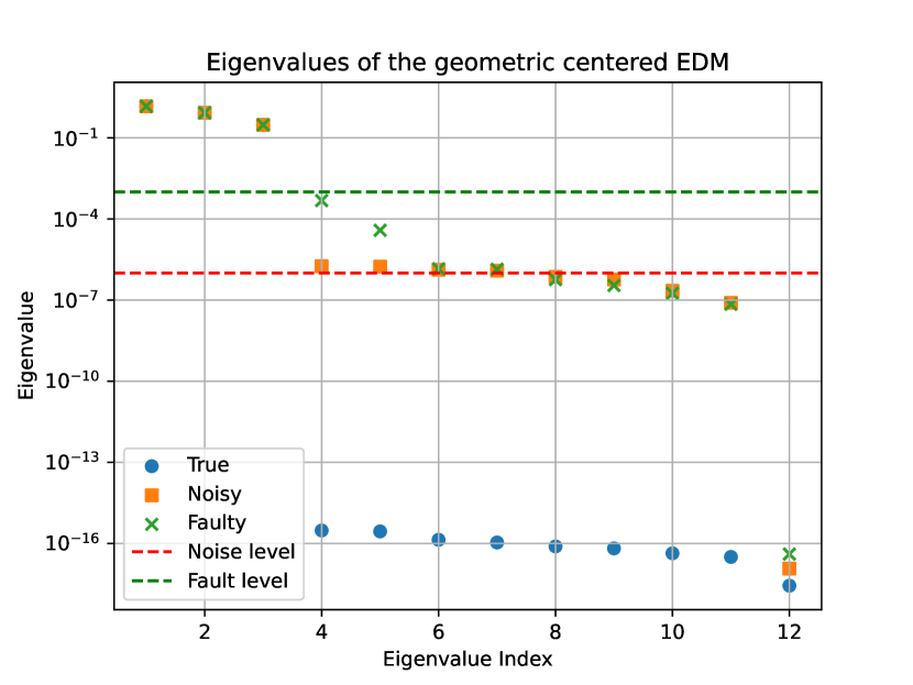
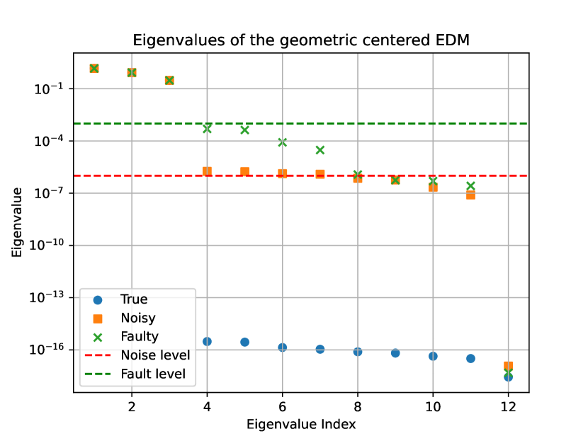
In (Knowles and Gao,, 2023), they observed that there are more than three nonzero singular values when the GCEDM is constructed from an EDM with fault satellites. An example is provided in Figure 1. However, mathematical proofs were not provided in their paper. In this section, we provide and prove several properties of the EDM and GCEDM that are corrupted with faults and measurement noises.
Proposition 2.1.
The rank of the EDM satisfies
| (6) |
Proof.
See Appendix A. ∎
Proposition 2.2.
The rank of the GCEDM satisfies
| (7) |
Proof.
See Appendix B. ∎
In practice, we observe that the relation in Proposition 2.2 holds with equality except for degenerate cases, such as those noted in Proposition 2.1. Specifically, the double centering will remove the sparsity pattern observed in Proposition 2.1, but it will not change the rank if . Moreover, although is positive semi-definite (Dokmanić et al.,, 2015), is not guaranteed to be positive semi-definite and we observe both positive and negative eigenvalues in practice.
Corollary 2.2.1.
The GCEDM constructed from an EDM with the edges corrupted by Gaussian noise almost surely has rank
| (8) |
Proof.
See Appendix C. ∎
2.3 Distribution of the singular values of the Geometric Centered EDM
The propositions proved in the previous sections indicate that we can detect fault satellites by observing the increase in the 4th and 5th singular values of the GCEDMs constructed from the ISR measurements. Following the work by (Knowles and Gao,, 2024), we use the following test statistics to monitor if a fault satellite exists in a given graph.
| (9) |
where is the th singular value of the geometric centered EDM. If the ISR measurements are completely noiseless, we can detect if a fault satellite exists within the graph by checking if of the GCEDMs is not 0, since GCEDMs have rank 3 when no fault exists. However, when the ISR measurements are noisy, the 4th and 5th singular values increase regardless of faults, as shown in Figure 1 and Corollary 2.2.1. Therefore, to detect faults under the presence of faults, we need to set a threshold that can separate the noise and fault. This threshold needs to be set based on the singular value distributions of the noisy (but non-fault) GCEDMs.
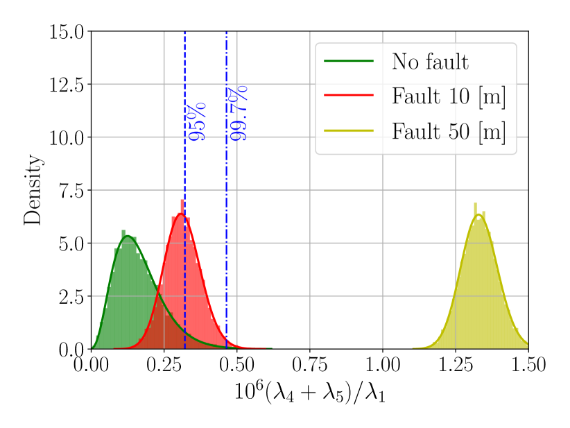
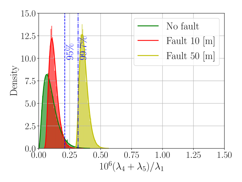
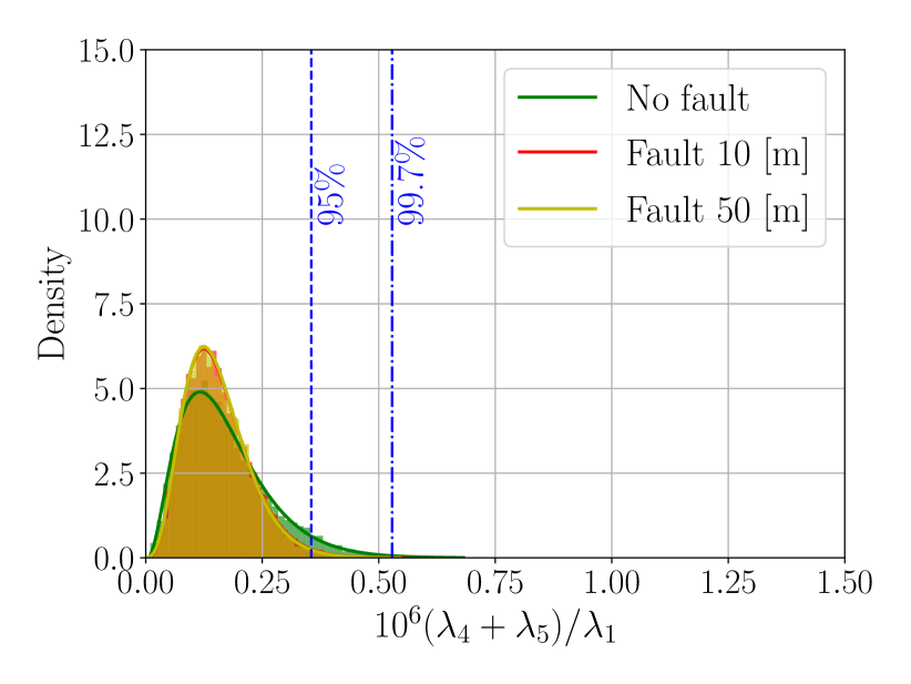
The distribution of the singular values of the three different patterns of noisy GCEDMs is shown in Figure 2. As illustrated in Figure 2, the distribution of is affected by the relative geometry of the satellites. When the satellites are spread in 3D space, the distribution of shifts to the right as the noise magnitude increases, as shown in Figure 2(a) and 2(b). In both non-fault and fault cases, the distribution can be well approximated by a gamma distribution. It is worth mentioning that for some geometries, it is not possible to distinguish fault by looking at the singular values because the distribution does not change in the presence of fault, as shown in Figure 2(c). This corresponds to the case where the non-fault satellites are in the same plane. This observation indicates that it is better to have satellites on diverse orbit planes to effectively detect faults.

3 Redundantly Rigid Graph-Based Fault Detection
3.1 Test Statistic Distribution Prediction Model
As mentioned in Section 2.3, the distribution of the test statistics of the non-fault noisy GCEDM can be approximated as a gamma distribution, where its shape parameters are determined by the relative geometry of the satellites. To detect faults by checking if exceeds a certain threshold, we are particularly interested in the tails of the distribution of the non-fault case. Therefore, our goal is to develop a model that can predict the parameters of tails of the (e.g., 99.7 percentile value ), given the ISR noise magnitude and the relative geometry.
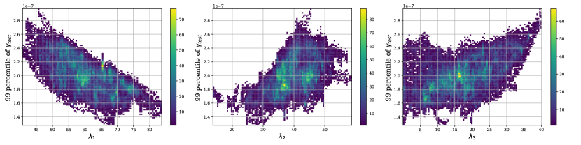
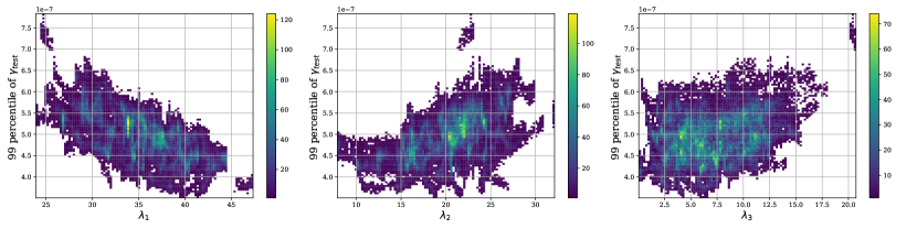
In this paper, we propose to use the first three singular values of the GCEDM and the first three columns of the orthogonal matrix of the singular value decomposition as the input to the model. These parameters remain almost constant under noise, when is sufficiently small compared to the ranges. Compared to using the elements of the GCEDM or EDM as the input, this input is invariant to the permutation of the nodes and is more robust to noise in the ranges. This results in an input dimension of , where is the number of satellites in the EDM. For this paper, we only use EDMs with 6 satellites for fault detection, so the input size is 21. An example of a 2D histogram that shows the mapping between the first three singular values and the 99.7 percentile of the test statistics () is shown in Figure 3. For fault detection, we need a model that can map the input to these percentile values, but from Figure 3, we observe that the map is nonlinear.
In this paper, we trained a neural network with 3 fully connected layers (Table 1) for the predictor
| (10) |
The training dataset is obtained by simulating the distribution of for 50000 noisy GCEDMs generated from 6 satellite subgraphs in the target constellation. Note that the training data can be generated by simulation because we assume we know the noise level and the configuration of the constellation beforehand. The predictor is trained separately for different constellations so that the predictors have good performance for the geometries that appear frequently in each constellation. In future work, we plan to investigate developing a more general predictor, so that it can generate outputs for arbitrary noise magnitudes and percentile values and a wider set of geometries.
| Layer | Input Size | Output Size | Activation |
|---|---|---|---|
| 1 | 21 | 128 | ReLU |
| 2 | 128 | 32 | ReLU |
| 3 | 32 | 1 | - |
3.2 Clique Listing
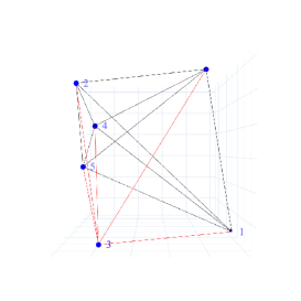
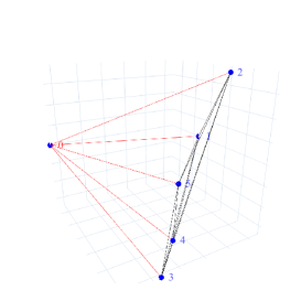
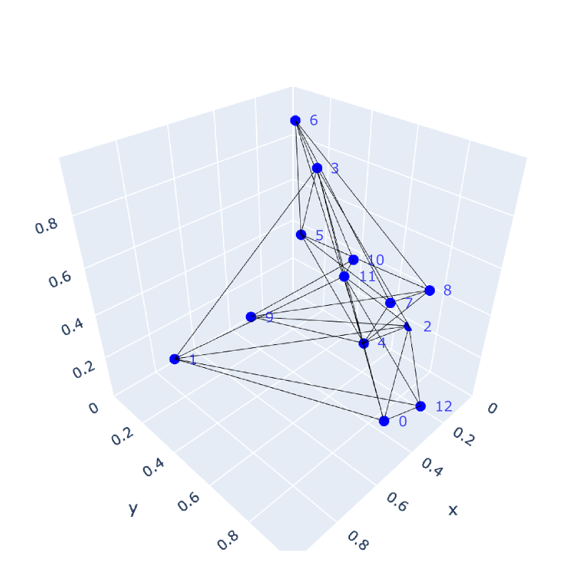
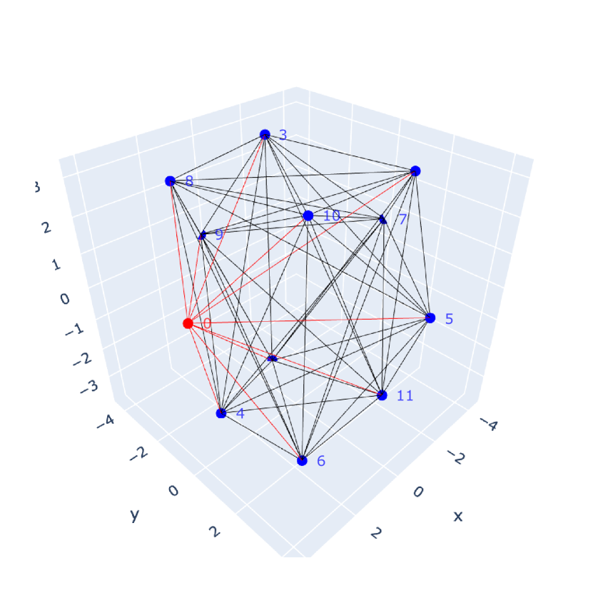
In order to construct an EDM and GCEDM, we need a set of range measurements between all pairs of satellites. However, due to the occultation by the planetary body and attitude constraints, the satellites in the constellation are not fully connected with ISRs in most cases. Therefore, the first step of the fault detection algorithm is to find a set of k-clique subgraphs, which are fully connected subgraphs of satellites. An example of 5-cliques subgraphs is shown in Figure 4.
Various exact algorithms to find all -cliques have been proposed (Li et al.,, 2020). In this paper, we used the Chiba-Nishizeki Algorithm (Albo) due to its simplicity of implementation (Chiba and Nishizeki,, 1985). For each node , Arbo expands the list of -cliques by recursively creating a subgraph induced by ’s neighbors. The readers are referred to (Li et al.,, 2020) for the pseudocode and summary of the -clique listing algorithm. Note that the clique finding algorithm does not have to be executed online. Since the availability of the ISRs can be predicted beforehand using a coarse predicted orbit, we can estimate the topology of the ISRs for future time epochs. We can compute the list of -cliques of the predicted topologies for future time epochs (e.g., one orbit), and uplink them to satellites intermittently. If some of these links were actually not available in orbit, we can remove the -cliques that contain the missing links from the list.

3.3 Online Fault Detection
Let be the list of all -cliques of the satellite network at time step , and the total number of satellites. We propose an online fault detection algorithm, which uses the trained predictor and . The main routine of the fault detection algorithm is shown in Algorithm 1. The overview of the detection algorithm is as follows. First, we judge whether a subgraph (-clique) contains a fault satellite by comparing the predicted and the observed statistics. If the subgraph is identified as a fault, then we look at the elements of (the 4th column of the orthogonal matrix obtained by SVD) to find which satellite within the subgraph is generating the fault. In particular, we look for the row with the largest magnitude. The satellite corresponding to this row is registered as a “fault candidate,” and a counter will be incremented. The satellite that has been registered as a fault candidate for most of the time is considered as a fault satellite and is removed from the entire graph. This procedure is repeated until there are no more faults. The key difference compared to the greedy-detection algorithm proposed by (Knowles and Gao,, 2024) is that we are using multiple subgraphs (EDMs) to detect faults. In addition, our algorithm has a predictor that can predict the test statistics for various graph geometries, compared to using a fixed threshold.
The proposed fault detection algorithm has several hyper-parameters that affect its performance. Below, we provide a guide on how the hyper-parameters should be determined.
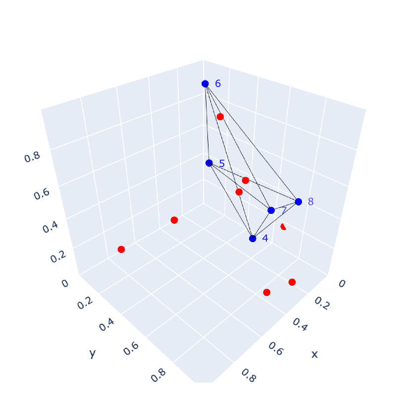
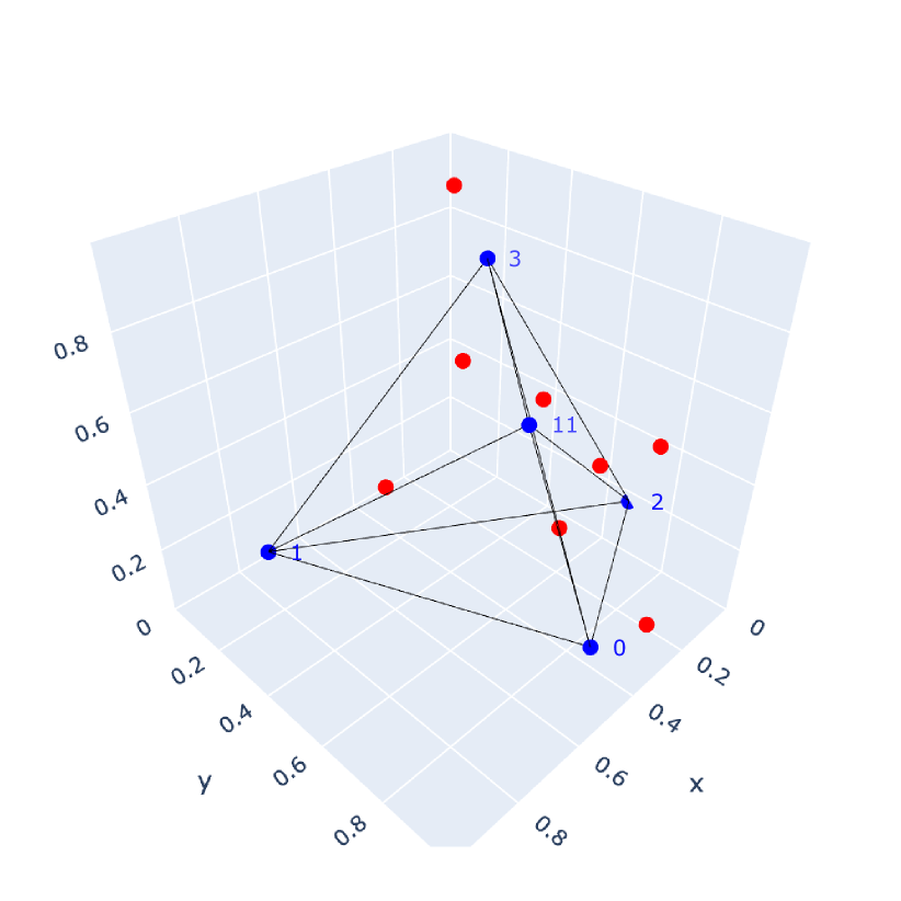
Clique Size : The size of the clique needs to be 5 or larger to compute the test statistics. To maximize the number of cliques that can be used for fault detection, we can use . However, from observation, we found that when we use , it is difficult to determine the fault satellite by looking at the index . Therefore, we propose to use cliques for fault detection. An example is shown in Figure 5.
Detection time interval : This controls the number of timesteps used to identify fault satellites. In general, the true positive rate will increase with larger DI, because the total number of subgraphs increases and the probability that large test statistics will be observed will increase.
Least required number of fault subgraphs : The algorithm will not detect faults if the total number of subgraphs detected as faults does not exceed this threshold. This is to avoid judging faults from a small number of samples and to reduce the false alarm rate.
Mimimum fault detection ratio : The algorithm will not detect any satellite as having a fault if the ratio of the number of times satellite detected as faults with respect to the total number of fault subgraphs does not exceed this threshold. This parameter needs to be set based on the maximum number of fault satellites (). In particular, we require

4 Satellite Fault Detection Simulation
4.1 Simulation Configuration and Evaluation Metrics
We validate our proposed algorithms for two different constellations around Mars and the Moon. The detailed configurations of the constellations are shown later in each section. For both simulation cases, the orbits are propagated in the two-body propagator without perturbations. The visibility of the links is calculated assuming that the links are visible when it is not occulted by the planetary body.
We run 500 Monte-Carlo analyses with randomly sampled initial time (within one orbital period) and a set of fault satellites. We tested 60 combinations of different detection and simulation parameters: 3 different numbers of fault satellites (1, 2, or 3), 5 different fault magnitudes ( = 5, 8, 10, 15, 20 m), and 4 different detection time intervals . The timestep between each detection for is set to 60 seconds. For the other hyper-parameters, we used . Note that the seed of the Monte-Carlo simulation is fixed so that the performance for different parameters is compared among the same conditions except the parameters.
We compute the following metrics to evaluate the performance of the detection algorithm
| (11) | ||||
| (12) | ||||
| (13) | ||||
| (14) |
where is the total number of true positives (fault satellite detected as fault), false negatives (fault satellite detected as non-fault), false positives (non-fault satellite detected as fault), and true negatives (non-fault satellite detected as non-fault).
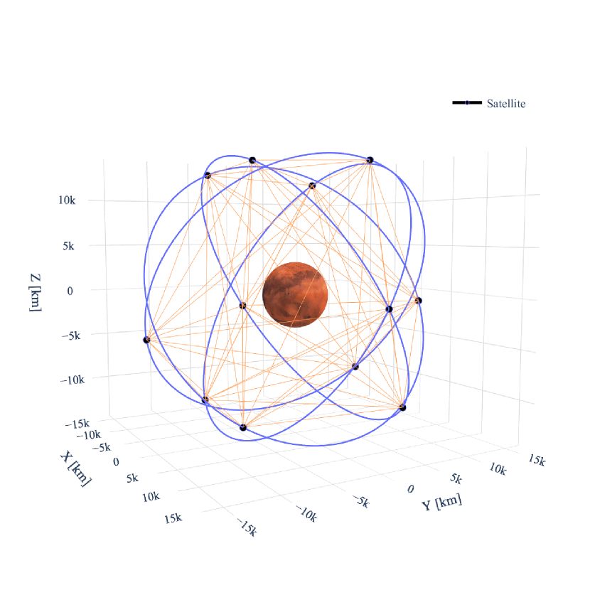
4.2 Case 1: Mars Walker Constellation
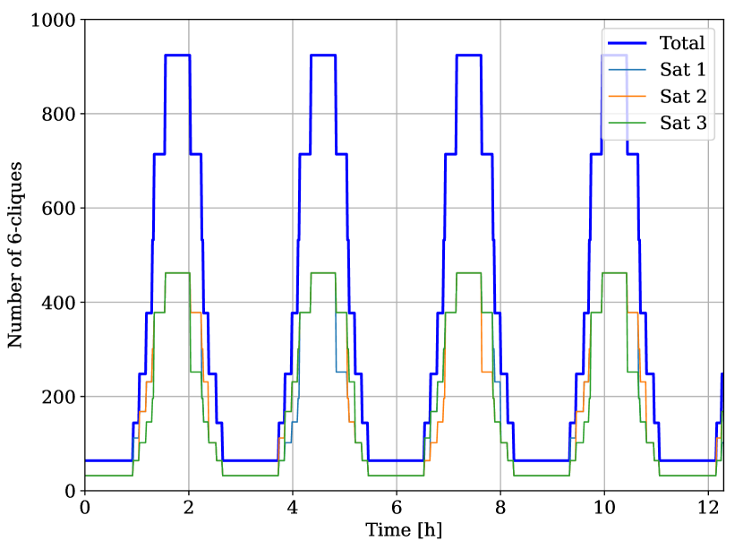
The first example is the Walker Delta constellation around Mars, with a total of 12 satellites equally spread to 4 different orbital planes. The orbital elements of the constellation are shown in Table 2. The constellation and the links at are shown in Figure 6(a). The number of 6-cliques in the constellation with the number of subgraphs containing satellite 1,2,3 (satellites in the first plane) is shown in Figure 6(b). For all timesteps, each satellite has at least 32 participations within a 6-clique that can be used for fault detection.
| Plane | Semi-Major Axis | Eccentricity | Inclination | RAAN | Argument of Periapsis | Mean Anomaly |
|---|---|---|---|---|---|---|
| [km] | [] | [deg] | [deg] | [deg] | [deg] | |
| 1 | 15850.55 | 0.0 | 60 | 0 | 0 | [0, 120, 240 ] |
| 2 | 15850.55 | 0.0 | 60 | 90 | 0 | [114.6, 234.6, 354.6] |
| 3 | 15850.55 | 0.0 | 60 | 180 | 0 | [229.2, 349.2, 109.2] |
| 4 | 15850.55 | 0.0 | 60 | -90 | 0 | [343.8, 103.8, 223.8] |
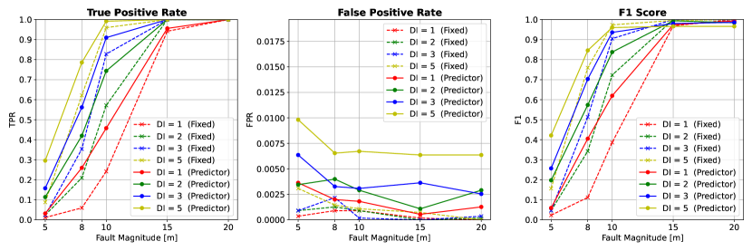
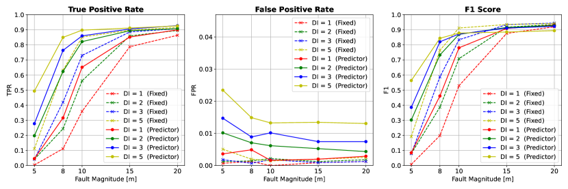
The fault detection results compared to the fixed threshold predictor are shown in Figure 7. For the fixed threshold predictor, was fixed to the 99.7 percentile value of the test statistics, which was computed from 50000 non-fault subgraphs that were randomly sampled from the entire simulation window. We observe that compared to the fixed threshold predictor, the machine learning predictor has a higher TPR, especially at lower fault magnitudes. This is because the predicted is less conservative compared to the fixed threshold, and considers more satellites (subgraphs) as fault candidates. However, the neural network predictor also has a higher FPR than the fixed threshold. This is because since the fixed threshold predictor is conservative, it only considers subgraphs of which the singular values and singular vectors of GCEDMs are largely perturbed, which is likely to be fault satellites. If it desired to make the FPR lower for the neural network predictor, we can do so by increasing the hyperparameter and .
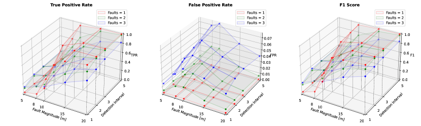
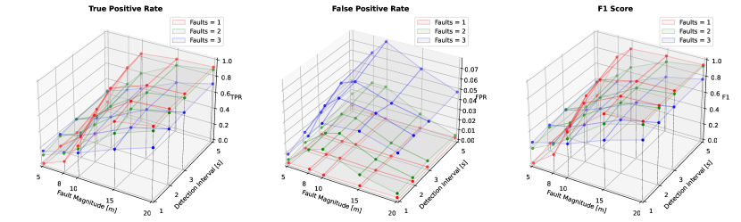
The sensitivity of fault magnitude, detection timesteps, and the number of faults to the detection metrics are shown in Figure 8. In general, the true positive rate is higher and the false positive rate is lower if we have a larger false magnitude and a smaller number of fault satellites, as it would be easier to detect fault subgraphs and distinguish which is the fault satellite. Increasing the detection time interval (DI) increases both the true positive rate and the false positive rate. Therefore, detection length can be used as a hyper-parameter to balance the true positive rate and false positive rate.
4.3 Case 2: Elliptical Lunar Frozen Orbit Constellation
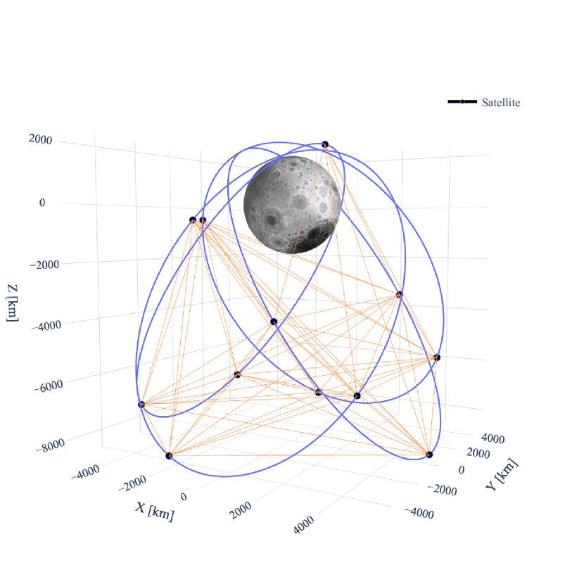
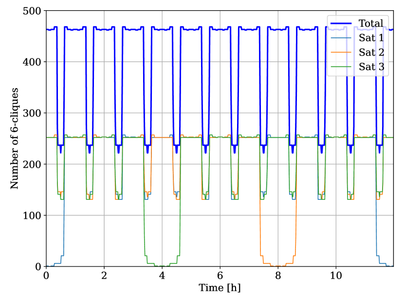
The second simulation scenario is the Elliptical Lunar Frozen Orbit (ELFO) constellation with a total of 12 satellites equally spread to 4 different orbital planes. The orbital elements of the constellation are shown in Table 3. The constellation and the links at are shown in Figure 9(a). The number of 6-cliques in the constellation with the number of subgraphs containing satellite 1,2,3 (satellites in the first plane) is shown in Figure 9(b). In this scenario, each satellite experiences a time window where they have zero or few self-containing subgraphs, where faults cannot be detected.
| Plane | Semi-Major Axis | Eccentricity | Inclination | RAAN | Argument of Periapsis | Mean Anomaly |
|---|---|---|---|---|---|---|
| [km] | [] | [deg] | [deg] | [deg] | [deg] | |
| 1 | 6142.4 | 0.6 | 57.7 | -90 | 90 | [0, 120, 240] |
| 2 | 6142.4 | 0.6 | 57.7 | 0 | 90 | [30, 150, 270] |
| 3 | 6142.4 | 0.6 | 57.7 | 90 | 90 | [60, 180, 300] |
| 4 | 6142.4 | 0.6 | 57.7 | 180 | 90 | [90, 210, 330] |
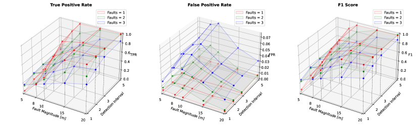
The fault detection results compared to the fixed threshold predictor are shown in Figure 10, and the sensitivity of fault magnitude, detection timesteps, and the number of faults to the detection metrics are shown in Figure 11. In general, the observed relationship between the parameters and the detection metrics is the same as in the Mars case. However, the TPR is capped around 0.92, because at any time there will be 1 satellite (8.3 of 12) located near the perilune, whose fault cannot be detected because of the limited number of self-containing subgraphs.

5 Conclusion
In this paper, we introduced a fault detection framework for autonomous satellite constellations using inter-satellite range (ISR) measurements. Our fault detection approach is based solely on the ISR measurements, and does not require the availability of precise ephemeris information. Compared to traditional fault monitoring methods that require ground station monitoring or precise ephemeris, our proposed method is suited for lunar and Martian environments where dedicated monitoring stations on the planetary surface would not be available.
In the paper, we start by providing mathematical proofs of several properties related to the rank of the EDM and GCEDM. Based on these properties, we demonstrated that satellite fault can be detected by analyzing the singular values and the singular vectors of the geometric centered Euclidean Distance Matrix (GCEDM) derived from ISR measurements. By combining a neural network predictor and the clique finding algorithm, the proposed fault detection framework can adapt the detection threshold to dynamic geometries and topologies, enhancing the robustness and reliability of fault detection. Through simulations of constellations around Mars and the Moon, we demonstrated the effectiveness of our fault detection framework in various configurations and organized the relationship between the environmental parameters and the detection metric.
This research marks a step towards establishing reliable operation of satellite constellations in extraterrestrial environments, which is the key architecture to support future exploration missions on the Moons or Mars. Future work will focus on refining the neural network predictor to accommodate more diverse and complex satellite constellations and combining the proposed algorithms with residual-based fault detection methods to further enhance the robustness and scalability of autonomous satellite fault detection.
acknowledgements
We acknowledge Derek Knowles for reviewing the paper. This material is based upon work supported by the National Science Foundation under Grant No. DGE-1656518 and CNS-2006162.
References
- Alawieh et al., (2016) Alawieh, M., Hadaschik, N., Franke, N., and Mutschler, C. (2016). Inter-satellite ranging in the low earth orbit. 2016 10th International Symposium on Communication Systems, Networks and Digital Signal Processing (CSNDSP), pages 1–6.
- Alireza Motevallian et al., (2015) Alireza Motevallian, S., Yu, C., and Anderson, B. D. (2015). On the robustness to multiple agent losses in 2D and 3D formations: MULTIPLE AGENT LOSSES IN 2D AND 3D FORMATIONS. International Journal of Robust and Nonlinear Control, 25(11):1654–1687.
- Chiba and Nishizeki, (1985) Chiba, N. and Nishizeki, T. (1985). Arboricity and subgraph listing algorithms. SIAM Journal on Computing, 14(1):210–223.
- Dokmanić et al., (2015) Dokmanić, I., Parhizkar, R., Ranieri, J., and Vetterli, M. (2015). Euclidean distance matrices: Essential theory, algorithms and applications. arXiv preprint.
- Israel et al., (2020) Israel, D. J., Mauldin, K. D., Roberts, C. J., Mitchell, J. W., Pulkkinen, A. A., Cooper, L. V. D., Johnson, M. A., Christe, S. D., and Gramling, C. J. (2020). LunaNet: A flexible and extensible lunar exploration communications and navigation infrastructure. In 2020 IEEE Aerospace Conference, pages 1–14.
- Knowles and Gao, (2023) Knowles, D. and Gao, G. (2023). Euclidean distance matrix-based rapid fault detection and exclusion. NAVIGATION: Journal of the Institute of Navigation, 70(1).
- Knowles and Gao, (2024) Knowles, D. and Gao, G. (2024). Greedy detection and exclusion of multiple faults using euclidean distance matrices. arXiv preprint arXiv:2404.12617.
- Li et al., (2020) Li, R., Gao, S., Qin, L., Wang, G., Yang, W., and Yu, J. X. (2020). Ordering heuristics for k-clique listing. Proceedings of the VLDB Endowment, 13:2536 – 2548.
- MISRA et al., (1993) MISRA, P., BAYLISS, E., LAFREY, R., PRATT, M., and MUCHNIK, R. (1993). Receiver autonomous integrity monitoring (raim) of gps and glonass. NAVIGATION, 40(1):87–104.
- National Aeronautics and Space Administration, (2022) National Aeronautics and Space Administration (2022). Lunar communications relay and navigation systems (lcrns) preliminary lunar relay services requirements document (srd).
- National Aeronautics and Space Administration, (2023) National Aeronautics and Space Administration (2023). Exploration systems development mission directorate moon-to-mars architecture definition document (esdmd-001).
- Rathje and Landsiedel, (2024) Rathje, P. and Landsiedel, O. (2024). Time difference of arrival extraction from two-way ranging.
- Rodríguez-Pérez et al., (2011) Rodríguez-Pérez, I., García-Serrano, C., Catalán Catalán, C., García, A. M., Tavella, P., Galleani, L., and Amarillo, F. (2011). Inter-satellite links for satellite autonomous integrity monitoring. Advances in Space Research, 47(2):197–212.
- Van Diggelen, (2009) Van Diggelen, F. S. T. (2009). A-gps: Assisted gps, gnss, and sbas. Artech house.
- Weiss et al., (2010) Weiss, M., Shome, P., and Beard, R. (2010). On-board gps clock monitoring for signal integrity. Proceedings of the 42nd Annual Precise Time and Time Interval Systems and Applications Meeting, pages 465–480.
- Wolf, (2000) Wolf, R. (2000). Onboard Autonomous Integrity Monitoring using Intersatellite Links. Proceedings of the 13th International Technical Meeting of the Satellite Division of The Institute of Navigation (ION GPS 2000).
- Working Group C, ARAIM Technical Subgroup, (2012) Working Group C, ARAIM Technical Subgroup (2012). Interim report. 1.
Appendix A Proof of Proposition 2.1
Proof.
As discussed in Dokmanić et al., (2015), the noiseless- and faultess-EDM, , based on a collection of points can be constructed with Equation (15).
| (15) |
where is the vector formed from the diagonal entries of . The first and last matrices of Equation (15) are rank 1 matrices by construction. These rank 1 matrix each contribute to the matrix rank except for degenerate cases where the points are equally spread apart (). The middle term includes the Gram matrix , which is rank except for degenerate cases where the points lie on a lower dimensional hyperplane (i.e., if the points lie on a plane). So, in line with Dokmanić et al., (2015), , where the condition holds with equality outside of the aforementioned degenerate cases.
During a fault, we encounter cross terms with the bias following Equation 16.
| (16) | ||||
Where is two times the elementwise square root of the corresponding entry in the EDM. As a matrix, we can write . We can write the bias term as a matrix as well. Both and are real, symmetric matrices. Then, we arrive at Equation (17).
| (17) |
where is the element-wise or Hadamard product. For the sake of illustration, consider the case with three faults realized at satellites for , without loss of generality.
| (18) |
In the rank-decomposition of , the column matrix has the first column has a one in each fault entry and a zero otherwise. This column spans all the fault-free columns. The remaining columns correspond to the columns in with faults and have a zero at the fault entry. achieves full rank when the number of faults reaches . In general, if and . By similar argument, since we will have one column indicating the fault entries and columns associated with the columns of with faults, which are the same columns as . This overall rank relationship often holds even if the faults are of different non-zero magnitudes. However, if the faults cancel out, the rank will drop. For example, in the case above, if and , then . Therefore, for arbitrary fault sizes. Nevertheless, the term can still be rank even if since the squaring can remove the linear cancellation.
However, the span of the columns of will generally span the columns . Again, for the sake of illustration, we extend the example above with faults at satellites for , without loss of generality.
| (19) | ||||
where are leftover terms from the row-reduction. In the rank-decomposition of , columns correspond to the columns in with faults and have a zero at the fault entry, just as before. However, now, one column is generally not enough to span the fault-free columns since the entries in are not linearly related. For example, is generally not a linear scaling of . These fault-free columns constitute an dimensional subspace, from which will need columns to fully span. achieves full rank when the number of faults reaches , where is the ceiling function. At that point, the subspace of fault-free columns is large enough that the fault columns will contribute to the span. Therefore, where we do not have equality when is degenerate (i.e., if the fault satellites are above or below a plane of fault-free satellites).
The columns needed to span are the same as those needed for , with the same sparsity pattern. Therefore, we will have
| (20) |
Lastly, the subspace spanned with the fault contributions is distinct from the subspace spanned by the EDM. Therefore,
| (21) |
where the equality holds in non-degenerate cases.
∎
Appendix B Proof of Proposition 2.2
Proof.
First, by rank inequality for arbitrary matrices and . The rank of the geometric centring matrix is . So, . However, this bound is too loose when there are few faults. Expanding the expression for geometric centering yields Equation (22).
| (22) | ||||
First, geometric centering removes the two rank 1 matrices, as shown in Equations (23) and (24) (Dokmanić et al.,, 2015).
| (23) | ||||
| (24) |
For the term, notice that the mean of the points is . Using this property yields Equation (25), which is a Gram matrix of the form for the point matrix centered about the origin (Dokmanić et al.,, 2015). This shift will not change the rank, meaning .
| (25) |
The remaining term is . By rank inequality,
| (26) |
So, we are left with
| (27) |
∎
Appendix C Proof of Proposition 2.2.1
Proof.
In terms of rank, the noise acts as many small faults on each satellite, with the same sparsity structure as in Proposition 2.1, almost surely with since there is zero probability mass that the randomly sampled noise is exactly zero or exactly cancel out. Using Proposition 2.2,
| (28) |
Therefore, succinctly, , almost surely. ∎