Stability of the TODA EQUATIONS RELATED TO A PERTURBED $R_{I}$ TYPE RECURRENCE RELATION

Abstract.

In this manuscript, a modified $R_{I}$ type recurrence relation is considered whose recurrence coefficients are perturbed by addition or multiplication of a constant. The perturbed system of recurrence coefficients is represented by Toda lattice equations, which are derived. These equations are then represented in a matrix form. With the help of this matrix representation, a known Lax pair is recovered. Inferences about the stability of resulting perturbed system of Toda equations are drawn based on numerical experiments.

1. Introduction

Orthogonal polynomials on the real line (OPRL) satisfy the following three term recurrence relation (TTRR)

$$\mathcal{R}_{n+1}(x)=(x-\beta_{n+1})\mathcal{R}_{n}(x)-\gamma_{n+1}\mathcal{R}_{n-1}(x),\quad\mathcal{R}_{-1}(x)=0,\quad\mathcal{R}_{0}(x)=1,\quad n\geq 0.$$ (1.1)

The two parameters $\beta_{n}$ and $\gamma_{n}$, involved in (1.1), can be modified by two fundamental mathematical operations, i.e., either by addition or by multiplication of a real number. The process is called co-recursion when the first term of the sequence $\{{\beta}_{n}\}_{n\geq 1}$ is perturbed by adding a constant, and co-dilation refers to the modification of the first term of the sequence $\{{\gamma}_{n}\}_{n\geq 1}$ by multiplying it with a constant [5, 12]. The perturbation in $\{{\beta}_{n}\}_{n\geq 1}$ at $n=k$ is termed generalized co-recursion, while the perturbation in $\{{\gamma}_{n}\}_{n\geq 1}$ at $n=k$ is termed generalized co-dilation. When both $\{{\beta}_{n}\}_{n\geq 1}$ and $\{{\gamma}_{n}\}_{n\geq 1}$ are perturbed at $n=k$, this condition is referred to as generalized co-modification [17]. In this context, co-modified OPRL or co-polynomials on the real line (COPRL), are introduced and studied in [4].

With regard to the measure $\psi(t)$ (a positive measure on the real line), let $\mathcal{P}_{n}(x;t)$ represent the monic orthogonal polynomials, where $t$ is the time variable that satisfies the following classical TTRR

$$\mathcal{R}_{n+1}(x;t)=(x-\beta_{n+1}(t))\mathcal{R}_{n}(x;t)-\gamma_{n+1}(t)\mathcal{R}_{n-1}(x;t),\quad n\geq 0,$$

$$\mathcal{R}_{-1}(x;t)=0,\qquad\mathcal{R}_{0}(x;t)=1,$$

and $d\psi(t)=e^{-tx}d\psi$. It is known [14] that the recurrence coefficients $\gamma_{n}(t)$ and $b_{n+1}(t)$ satisfy the semi-infinite Toda lattice equations of motion

$$\dot{\gamma}_{n}(t) =\gamma_{n}(t)[\beta_{n-1}(t)-\beta_{n}(t)],$$

$$\dot{\beta}_{n}(t) =\gamma_{n}(t)-\gamma_{n+1}(t),\quad n\geq 1,$$ (1.2)

with initial conditions $\beta_{0}(t)=1$, $\gamma_{1}(t)=0$, $\gamma_{n}(0)=\gamma_{n}$ and $\beta_{n}(0)=\beta_{n}$, where $\dot{f}$ represents the differentiation of $f$ with respect to $t$ in this case.

Consider the recurrence

$$\mathcal{P}_{n+1}(z)=(z-c_{n+1})\mathcal{P}_{n}(z)-\lambda_{n+1}(z-a_{n+1})\mathcal{P}_{n-1}(z),\quad n\geq 0,$$ (1.3)

$$\mathcal{P}_{-1}(z)=0,\qquad\mathcal{P}_{0}(z)=1,$$

where $\{{\lambda}_{n}\}_{n\geq 1}$ and $\{c_{n}\}_{n\geq 1}$ are real sequences. A rational function $\psi_{n}(z)=\frac{\mathcal{P}_{n}(z)}{\prod_{j=1}^{n}(z-a_{j})}$ exists if $\lambda_{n}\neq 0$ and $\mathcal{P}_{n}(a_{n})\neq 0$ for $n\geq 1$, as was proven in [15, Theorem 2.1]. Further, we have a linear moment functional $\mathcal{L}$ such that the orthogonality relations

$$\mathcal{L}[a_{0}]\neq 0,\quad\mathcal{L}\left[z^{k}\psi_{n}(z)\right]\neq 0,\quad 0\leq k<n,$$

hold. According to [15], (1.3) is called the recurrence relation of $R_{I}$ type, and $\mathcal{P}_{n}(z),n\geq 1$, generated by it are called $R_{I}$ polynomials. Furthermore, (1.3) is associated with a non-trivial positive measure of orthogonality defined either on the unit circle or on a subset of the real line whenever $a_{n}=0$, $n\geq 1$ [21]. Fixing $a_{n}=0$ and $z\in\mathbb{R}$, we arrive at a special form of $R_{I}$ type recurrence relation

$$\mathcal{P}_{n+1}(x)=(x-c_{n+1})\mathcal{P}_{n}(x)-\lambda_{n+1}x\mathcal{P}_{n-1}(x),\quad n\geq 1,$$ (1.4)

$$\mathcal{P}_{-1}(x)=0,\qquad\mathcal{P}_{0}(x)=1$$

satisfied by orthogonal Laurent polynomials, where $\{c_{n}\}_{n\geq 1}$ is a real sequence and $\{{\lambda}_{n}\}_{n\geq 1}$ are positive real numbers. We refer to [3, 7, 16] for some recent progress related to $R_{I}$ type recurrence relations and $R_{I}$ polynomials. The modification of recurrence coefficients in (1.3) and (1.4) at $n=k$, defined as

$$c_{k+1} \rightarrow c_{k+1}+\mu_{k+1},\qquad\rm(generalized~{}co-recursion)$$ (1.5)

$$\lambda_{k+1} \rightarrow\nu_{k+1}\lambda_{k+1},\hskip 14.22636pt\qquad\rm(generalized~{}co-dilation),$$ (1.6)

where $k$ is a fixed non-negative integer, has been studied in [20] and resultant polynomials are termed as co-polynomials of $R_{I}$ type.

Let $\mathfrak{N}$ denote the moment functional such that the moments given by $\mathfrak{N}[x^{k}e^{-t(px+\frac{q}{x})}]$ exists where $p,q\in\mathbb{C}$ and $k\in\mathbb{Z}$ and . The parametrized moment functional $\mathfrak{N}^{(t)}$ for $t\geq 0$ is such that

$$\mathfrak{N}^{(t)}[x^{k}]=\mathfrak{N}[x^{k}e^{-t(px+\frac{q}{x})}].$$ (1.7)

Following [23], if $\mathcal{P}_{n}(x;t)$ satisfy

$$\mathcal{P}_{n+1}(x;t)=(x-c_{n+1}(t))\mathcal{P}_{n}(x;t)-\lambda_{n+1}(t)x\mathcal{P}_{n-1}(x;t),\quad n\geq 1,$$ (1.8)

with $\mathcal{P}_{0}(x;t)=1$ and $\mathcal{P}_{1}(x;t)=x-c_{1}(t)$. Then, the recurrence coefficients $\lambda_{n}(t)$ and $c_{n}(t)$ satisfy relativistic Toda equations

$$\dot{\lambda}_{n}=\lambda_{n}\left(\dfrac{1}{c_{n-1}}-\dfrac{1}{c_{n}}\right),\quad\dot{c}_{n}=c_{n}\left(\dfrac{\lambda_{n+1}}{c_{n+1}c_{n}}-\dfrac{\lambda_{n}}{c_{n}c_{n-1}}\right),\quad n\geq 1,$$ (1.9)

when $q=1$ and $p=0$, and

$$\dot{\lambda}_{n}=\lambda_{n}(\lambda_{n-1}+c_{n-1}-\lambda_{n+1}-c_{n}),\quad\dot{c}_{n}=c_{n}(\lambda_{n}-\lambda_{n+1}),\quad n\geq 1,$$ (1.10)

when $q=0$ and $p=1$. Moreover, using a more general form of (1.8) given as

$$\mathcal{P}_{n+1}(x;t)=(x-c_{n+1}(t))\mathcal{P}_{n}(x;t)-\lambda_{n+1}(t)(x-a_{n}(t))\mathcal{P}_{n-1}(x;t),\quad n\geq 1,$$

with $\mathcal{P}_{0}(x;t)=1$ and $\mathcal{P}_{1}(x;t)=x-c_{1}(t)$, the relativistic Toda equations (1.9) and (1.10) have been further extended to generalized relativistic Toda equations (see [23]) that are expressed as

$$\dot{c}_{n}=a_{n}\lambda_{n}-a_{n+1}\lambda_{n+1}+c_{n}(\lambda_{n+1}-\lambda_{n}),$$

$$\dot{\lambda}_{n}=\lambda_{n}(\lambda_{n+1}-\lambda_{n-1}+c_{n}-c_{n-1}),\quad n\geq 1.$$

In a recent work [2], extended relativistic Toda equations have been derived corresponding to the L-orthogonal polynomials (1.8) via duo-directional modification $px+q/x$ in (1.7). We refer to [11, 9] and references therein for some recent advancements in the theory of Toda equations. This manuscript aims to investigate the consequences of perturbing the recurrence coefficients in (1.8) on the Toda equations of motion. Perturbed extended relativistic Toda equations are the name given to the equations so derived. The Toda lattice equation for $n=k$ is found by considering a single perturbation of the recurrence coefficient; this is the focus of Section 2. A Lax pair for extended relativistic Toda equations, discussed in [2], is also recovered. A natural question arises regarding the stability of such a perturbed system. This aspect has been addressed in this work, with Section 3 dedicated to investigating how the system’s dynamics are influenced and whether the perturbed system demonstrates stable behavior. To the author’s knowledge, such a study has not been conducted in the existing literature for Toda equations.

2. Toda lattice equations

2.1. Perturbed extended relativistic Toda equations

The monic polynomials $\mathcal{\hat{P}}_{n}(x;t)$ of degree $n$ satisfy

$$\mathcal{\hat{P}}_{n+1}(x;t)=(x-\hat{c}_{n+1}(t))\mathcal{\hat{P}}_{n}(x;t)-\hat{\lambda}_{n+1}(t)x\mathcal{\hat{P}}_{n-1}(x;t),\quad n\geq 1,$$ (2.1)

where $\hat{c}_{n+1}(t)$ and $\hat{\lambda}_{n+1}(t)$ denote the modification of recurrence coefficients as described in (1.5) and (1.6), e.g.,

$$\hat{c}_{k+1}(t)={c}_{k+1}(t)-\mu_{k+1}(t),\quad\hat{\lambda}_{k+1}(t)=\nu_{k+1}(t){\lambda}_{k+1}(t),\quad{\rm for}~{}~{}n=k,$$

$$\hat{c}_{n+1}(t)={c}_{n+1}(t),\hskip 62.59596pt\hat{\lambda}_{n+1}(t)={\lambda}_{n+1}(t),\hskip 45.52458pt{\rm for}~{}~{}n\neq k.$$

Lemma 1.

If $\hat{\rho}_{n}=\mathfrak{\hat{N}}^{(t)}[x\mathcal{\hat{P}}_{n}(x;t)]$ for $n\geq 0$, then

$$\hat{\rho}_{n}=\hat{\sigma}_{n,n}(t)\sum_{i=1}^{n+1}[\hat{c}_{i}(t)+\hat{\lambda}_{i+1}(t)],\quad n\geq 0.$$

The proof of the above lemma is similar to the one given in [2] and hence omitted. The next result provides a perturbed analogue of Theorem $1$ given in [2].

Theorem 2.1.

Let $\mathcal{P}_{n}(x;t)$ be the L-orthogonal polynomials generated by (1.8) and $\mathcal{\hat{P}}_{n}(x;t)$ be its perturbed version defined by (2.1). The recurrence coefficients ${\lambda}_{n}(t)$ and $c_{n}(t)$ satisfy the following perturbed extended relativistic Toda equations:

$$\dfrac{\dot{c}_{k}}{c_{k}}=p({\lambda}_{k}-\nu_{k+1}{\lambda}_{k+1})+q\left(\dfrac{\nu_{k+1}{\lambda}_{k+1}}{(c_{k+1}-\mu_{k+1})c_{k}}-\dfrac{{\lambda}_{k}}{c_{k}c_{k-1}}\right),\quad n=k,$$

$$\dot{c}_{k+1}=\dot{\mu}_{k+1}+p(c_{k+1}-\mu_{k+1})(\nu_{k+1}{\lambda}_{k+1}-{\lambda}_{k+2})+q\left(\dfrac{{\lambda}_{k+2}}{c_{k+2}}-\dfrac{\nu_{k+1}{\lambda}_{k+1}}{c_{k}}\right),\quad n=k+1,$$

$$\dfrac{\dot{c}_{k+2}}{c_{k+2}}=p({\lambda}_{k+2}-{\lambda}_{k+3})+q\left(\dfrac{{\lambda}_{k+3}}{c_{k+2}c_{k+3}}-\dfrac{{\lambda}_{k+2}}{(c_{k+1}-\mu_{k+1})c_{k+2}}\right),\quad n=k+2,$$

$$\dfrac{\dot{c}_{n}}{c_{n}}=p({\lambda}_{n}-{\lambda}_{n+1})+q\left(\dfrac{{\lambda}_{n+1}}{c_{n+1}c_{n}}-\dfrac{{\lambda}_{n}}{c_{n}c_{n-1}}\right),\quad otherwise,$$ (2.2)

and for $n=k$,

$$\dfrac{\dot{\lambda}_{k+1}}{{\lambda}_{k+1}}=-\dfrac{\dot{\nu}_{k+1}}{{\nu}_{k+1}}-p({\lambda}_{k+2}+c_{k+1}-\mu_{k+1}+(\nu_{k+1}-1)\lambda_{k+1}-c_{k}-\lambda_{k})-q\left(\dfrac{1}{c_{k+1}-\mu_{k+1}}-\dfrac{1}{c_{k}}\right),$$

$$\dfrac{\dot{\lambda}_{k+2}}{{\lambda}_{k+2}}=-p[\lambda_{k+3}+c_{k+2}-(c_{k+1}-\mu_{k+1})-\nu_{k+1}\lambda_{k+1}]-q\left(\dfrac{1}{c_{k+2}}-\dfrac{1}{c_{k+1}-\mu_{k+1}}\right),\quad n=k+1,$$

$$\dfrac{\dot{\lambda}_{n}}{{\lambda}_{n}}=p(\lambda_{n-1}+c_{n-1}-\lambda_{n+1}-c_{n})+q\left(\dfrac{1}{c_{n-1}}-\dfrac{1}{c_{n}}\right),\quad otherwise,$$ (2.3)

with initial conditions $c_{0}(t)=1$, $\lambda_{0}(t)=-1$ and $\lambda_{1}(t)=0$. Here, variable $t$ has been omitted for simplicity.

Proof.

The sequences $\mathcal{P}_{n}(x;t)$ and $\mathcal{\hat{P}}_{n}(x;t)$ satisfy the following L-orthogonality conditions

$$\mathfrak{\hat{N}}^{(t)}[x^{-n+j}\mathcal{\hat{P}}_{n}(x;t)]=0,\quad j=0,1,\ldots n-1,$$ (2.4)

$$\mathfrak{N}^{(t)}[x^{-n+r}\mathcal{P}_{n}(x;t)]=0,\quad r=0,1,\ldots n-1.$$

Let $\mathcal{P}_{n}(x;t)=\sum_{j=0}^{n}a_{n,j}x^{j}$ and $\mathcal{\hat{P}}_{n}(x;t)=\sum_{j=0}^{n}\hat{a}_{n,j}x^{j}$ where $a_{n,n}=1$ and $\hat{a}_{n,n}=1$. Then $\sigma_{n,-1}(t)=\mathfrak{N}^{(t)}[x^{-n-1}\mathcal{P}_{n}(x;t)]$, $\hat{\sigma}_{n,n}(t)=\mathfrak{N}^{(t)}[\mathcal{P}_{n}(x;t)]$, $\hat{\sigma}_{n,-1}(t)=\mathfrak{\hat{N}}^{(t)}[x^{-n-1}\mathcal{\hat{P}}_{n}(x;t)]$ and $\hat{\sigma}_{n,n}(t)=\mathfrak{\hat{N}}^{(t)}[\mathcal{\hat{P}}_{n}(x;t)]$. Clearly, for $n<k$, $\hat{\sigma}_{n,n}(t)=\sigma_{n,n}(t)$ and $\hat{\sigma}_{n,-1}(t)=\sigma_{n,-1}(t)$. From this, we have

$$\begin{split}&\hat{\sigma}_{k,-1}(t)=-\dfrac{\nu_{k+1}(t)\lambda_{k+1}(t)}{{c}_{k+1}(t)-\mu_{k+1}(t)}\sigma_{k-1,-1}(t),\\ &\hat{\sigma}_{n,-1}(t)=-\dfrac{\lambda_{n+1}(t)}{{c}_{n+1}(t)}\hat{\sigma}_{n-1,-1}(t),\quad n>k,\end{split}$$ (2.5)

and

$$\begin{split}&\hat{\sigma}_{k,k}(t)=\nu_{k+1}(t)\lambda_{k+1}(t)\sigma_{k-1,k-1}(t),\\ &\hat{\sigma}_{n,n}(t)=\lambda_{n+1}(t)\hat{\sigma}_{n-1,n-1}(t),\quad n>k.\end{split}$$ (2.6)

From (1.8) and (2.1), we have

$$a_{n,0}(t)=(-1)^{n}c_{n}(t)c_{n-1}(t)\ldots c_{2}(t)c_{1}(t),\quad n\geq 1,$$

$$\hat{a}_{n,0}(t)=(-1)^{n}\hat{c}_{n}(t)\hat{c}_{n-1}(t)\ldots\hat{c}_{2}(t)\hat{c}_{1}(t),\quad n\geq 1,$$

which implies

$$\begin{split}&\hat{a}_{n,0}(t)=a_{n,0}(t),\quad n\leq k,\quad\hat{a}_{k+1,0}(t)=-({c}_{k+1}(t)-\mu_{k+1}(t))a_{k,0}(t),\\ \text{and}\quad&\hat{a}_{n,0}(t)=-c_{n}(t)\hat{a}_{n-1,0}(t),\quad n>k+1.\end{split}$$ (2.7)

Again, using (2.1), we obtain

$$\hat{c}_{n+1}(t)+\hat{\lambda}_{n+1}(t)=\hat{a}_{n,n-1}(t)-\hat{a}_{n+1,n}(t),\quad n\geq 1,$$

which implies

$$\begin{split}&c_{n+1}(t)+\lambda_{n+1}(t)={a}_{n,n-1}(t)-{a}_{n+1,n}(t),\quad n<k,\\ &c_{k+1}(t)+\lambda_{k+1}(t)-\mu_{k+1}(t)+(\nu_{k+1}(t)-1)\lambda_{k+1}(t)={a}_{k,k-1}(t)-\hat{a}_{k+1,k}(t),\\ &c_{n+1}(t)+\lambda_{n+1}(t)=\hat{a}_{n,n-1}(t)-\hat{a}_{n+1,n}(t),\quad n>k.\end{split}$$ (2.8)

From (2.4), we get

$$\mathfrak{\hat{N}}^{(t)}[x^{-n}\mathcal{\hat{P}}_{n-1}(x;t)\mathcal{\hat{P}}_{n}(x;t)]=0,\quad n\geq 1.$$

Differentiating this with respect to (w.r.t.) $t$, we have

$$\mathfrak{\hat{N}}^{(t)} [x^{-n}\mathcal{\dot{\hat{P}}}_{n-1}(x;t)\mathcal{\hat{P}}_{n}(x;t)]+\mathfrak{\hat{N}}^{(t)}[x^{-n}\mathcal{\hat{P}}_{n-1}(x;t)\mathcal{\dot{\hat{P}}}_{n}(x;t)]$$

$$-\mathfrak{\hat{N}}^{(t)}[x^{-n}\left(px+\frac{q}{x}\right)\mathcal{\hat{P}}_{n-1}(x;t)\mathcal{\hat{P}}_{n}(x;t)]=0,\quad n\geq 1.$$ (2.9)

where $\mathcal{\dot{\hat{P}}}_{n}(x;t)=\dfrac{\partial}{\partial t}\mathcal{\hat{P}}_{n}(x;t)$. Again from (2.4), we get $\mathfrak{\hat{N}}^{(t)}[x^{-n}\mathcal{\dot{\hat{P}}}_{n-1}(x;t)\mathcal{\hat{P}}_{n}(x;t)]=0$. Further, since $\mathcal{\dot{\hat{P}}}_{n}(x;t)=\sum_{j=0}^{n-1}\dot{\hat{a}}_{n,j}x^{j}$ , we obtain

$$\mathfrak{\hat{N}}^{(t)}[x^{-n}\mathcal{\hat{P}}_{n-1}(x;t)\mathcal{\dot{\hat{P}}}_{n}(x;t)]=\dot{\hat{a}}_{n,0}(t)\hat{\sigma}_{n-1,-1}(t),$$

$$\mathfrak{\hat{N}}^{(t)}[x^{-n+1}\mathcal{\hat{P}}_{n-1}(x;t)\mathcal{\hat{P}}_{n}(x;t)]=\hat{\sigma}_{n,n}(t),$$

$$\mathfrak{\hat{N}}^{(t)}[x^{-n-1}\mathcal{\hat{P}}_{n-1}(x;t)\mathcal{\hat{P}}_{n}(x;t)]=\hat{\sigma}_{n,n}(t)=\hat{a}_{n-1,0}(t)\hat{\sigma}_{n,-1}(t),\quad n\geq 1.$$

Putting these values in (2.1), we have

$$\dot{\hat{a}}_{n,0}(t)\hat{\sigma}_{n-1,-1}(t)=p\hat{\sigma}_{n,n}(t)+q\hat{a}_{n-1,0}(t)\hat{\sigma}_{n,-1}(t),\quad n\geq 1.$$

Substituting (2.5), (2.6) and (2.7) in the above expression, we conclude

$$\sum_{i=1}^{n}\dfrac{\dot{c}_{i}(t)}{c_{i}(t)} =-p\lambda_{n+1}(t)+q\dfrac{\lambda_{n+1}(t)}{c_{n+1}(t)c_{n}(t)},\quad n<k,$$ (2.10)

$$\sum_{i=1}^{k}\dfrac{\dot{c}_{i}(t)}{c_{i}(t)} =-p\nu_{k+1}(t)\lambda_{k+1}(t)+q\dfrac{\nu_{k+1}(t)\lambda_{k+1}(t)}{(c_{k+1}(t)-\mu_{k+1}(t))c_{k}(t)},\quad n=k,$$ (2.11)

$$\sum_{i=1}^{k+1}\dfrac{\dot{\hat{c}}_{i}(t)}{\hat{c}_{i}(t)} =\sum_{i=1}^{k}\dfrac{\dot{c}_{i}(t)}{c_{i}(t)}+\dfrac{\dot{c}_{k+1}(t)-\dot{\mu}_{k+1}(t)}{c_{k+1}(t)-\mu_{k+1}(t)}=-p\lambda_{k+2}(t)$$

$$+q\dfrac{\lambda_{k+2}(t)}{{(c_{k+1}(t)-\mu_{k+1}(t))c_{k+2}(t)}},\quad n=k+1,$$ (2.12)

$$\sum_{i=1}^{n}\dfrac{\dot{\hat{c}}_{i}(t)}{\hat{c}_{i}(t)} =-p\lambda_{n+1}(t)+q\dfrac{\lambda_{n+1}(t)}{c_{n+1}(t)c_{n}(t)},\quad n>k+1.$$ (2.13)

Substraction of (2.12) from (2.13) for $n=k+2$, (2.11) from (2.12), and (2.10) from (2.11) for $n=k-1$ yields the first four relations given in the hypothesis of the Theorem 2.1.

Note that (2.4) implies $\mathfrak{\hat{N}}^{(t)}[x^{-n}\mathcal{\hat{P}}^{2}_{n}(x;t)]=\hat{\sigma}_{n,n}(t)$. Differentiating this w.r.t. $t$ and substituting $\mathfrak{\hat{N}}^{(t)}[x^{-n}\mathcal{\dot{\hat{P}}}_{n}(x;t)\mathcal{\hat{P}}_{n}(x;t)]=0$, we obtain

$$-\mathfrak{\hat{N}}^{(t)}[x^{-n}\left(px+\frac{q}{x}\right)\mathcal{\hat{P}}^{2}_{n}(x;t)]=\dot{\hat{\sigma}}_{n,n}(t),\quad n\geq 1.$$ (2.14)

Now, from (2.4), we observe that

$$\mathfrak{\hat{N}}^{(}t)[x^{-n-1}\mathcal{\hat{P}}^{2}_{n}(x;t)]=\hat{a}_{n,0}(t)\hat{\sigma}_{n,-1}(t),\quad n\geq 0,$$ (2.15)

and using Lemma 1, we get

$$\mathfrak{\hat{N}}^{(}t)[x^{-n+1}\mathcal{\hat{P}}^{2}_{n}(x;t)]=\hat{a}_{n,n-1}(t)\hat{\sigma}_{n,n}(t)+\hat{\sigma}_{n,n}(t)\sum_{i=1}^{n+1}[\hat{c}_{i}(t)+\hat{\lambda}_{i+1}(t)],\quad n\geq 0.$$ (2.16)

Using (2.8), we obtain

$$\begin{split}&{a}_{n,n-1}(t)+\sum_{i=1}^{n+1}[{c}_{i}(t)+{\lambda}_{i+1}(t)]={\lambda}_{n+2}(t)+{\lambda}_{n+1}(t)+{c}_{n+1}(t),\quad n<k,\\ &{a}_{k,k-1}(t)+\sum_{i=1}^{n+1}[\hat{c}_{i}(t)+\hat{\lambda}_{i+1}(t)]={\lambda}_{k+2}(t)+\nu_{k+1}(t){\lambda}_{k+1}(t)+{c}_{k+1}(t)-\mu_{k+1}(t),\quad n=k,\\ &\hat{a}_{n,n-1}(t)+\sum_{i=1}^{n+1}[\hat{c}_{i}(t)+\hat{\lambda}_{i+1}(t)]={\lambda}_{n+2}(t)+{\lambda}_{n+1}(t)+{c}_{n+1}(t),\quad n>k.\end{split}$$ (2.17)

Substituting (2.15), (2.16) and (2.17) in (2.14) and dividing by $\hat{\sigma}_{n,n}(t)$, we conclude that

$$-p[\lambda_{n+2}(t) +\lambda_{n+1}(t)+c_{n+1}(t)]-\dfrac{q}{c_{n+1}(t)}=\dfrac{\dot{\sigma}_{0,0}(t)}{\sigma_{0,0}(t)}+\sum_{i=2}^{n+1}\dfrac{\dot{\lambda}_{i}(t)}{\lambda_{i}(t)},\quad n<k,$$ (2.18)

$$-p[\lambda_{k+2}(t) +\nu_{k+1}\lambda_{k+1}(t)+c_{k+1}(t)-\mu_{k+1}(t)]-\dfrac{q}{c_{k+1}(t)-\mu_{k+1}(t)}$$

$$=\dfrac{\dot{\sigma}_{0,0}(t)}{\sigma_{0,0}(t)}+\sum_{i=2}^{n+1}\dfrac{\dot{\lambda}_{i}(t)}{\lambda_{i}(t)}+\dfrac{\dot{\nu}_{k+1}(t)}{\nu_{k+1}(t)}=\dfrac{\dot{\sigma}_{0,0}(t)}{\sigma_{0,0}(t)}+\sum_{i=2}^{n+1}\dfrac{\dot{\hat{\lambda}}_{i}(t)}{\hat{\lambda}_{i}(t)},\quad n=k,$$ (2.19)

$$-p[\lambda_{n+2}(t) +\lambda_{n+1}(t)+c_{n+1}(t)]-\dfrac{q}{c_{n+1}(t)}=\dfrac{\dot{\sigma}_{0,0}(t)}{\sigma_{0,0}(t)}+\sum_{i=2}^{n+1}\dfrac{\dot{\hat{\lambda}}_{i}(t)}{\hat{\lambda}_{i}(t)},\quad n>k.$$ (2.20)

Substraction of (2.20) from (2.19) for $n=k+1$ and (2.18) for $n=k-1$ from (2.19) yields the last three relations given in the hypothesis of the Theorem 2.1. This completes the proof. ∎

Corollary 2.1.

With the help of Theorem 2.1, the perturbed version of (1.9) and (1.10), the relativistic Toda equations, can be obtained by substituting either $p=0$, $q=1$ or $p=1$, $q=0$.

Remark 2.1.

Clearly, we get [2, Theorem 1] by substituting $\mu_{k+1}=0$ and $\nu_{k+1}=1$ in Theorem 2.1.

Remark 2.2.

It is noteworthy that a single modification in the recurrence coefficients for $n=k$ affects three Toda equation of motion for $c_{n}$, i.e., for $n=k$, $n=k+1$ and $n=k+2$, and two Toda equation of motion for $\lambda_{n}$ i.e., for $n=k$ and $n=k+1$, with the remaining levels unchanged.

2.2. Recovering a Lax pair from a matrix differential representation

A matrix differential equation corresponding to perturbed extended relativistic Toda equations given in Theorem 2.1 is derived in this subsection, which is further used to recover a Lax pair presented in [2]. A matrix differential equation of the form

$$\mathcal{\dot{S}}=[\mathcal{S},\mathcal{T}]=\mathcal{S}\mathcal{T}-\mathcal{T}\mathcal{S},$$

is called a Lax representation for Toda lattice equations (1) and the pair $\{\mathcal{S},\mathcal{T}\}$ is called a Lax pair [10] where $\mathcal{S}$ and $\mathcal{T}$ are semi-infinite tri-diagonal and strictly lower Hessenberg matrices in case of (1) [18], lower and upper bi-diagonal matrices in case of relativistic Toda equations (1.9) and (1.10) [8], and upper Hessenberg and tri-diagonal matrices in case of extended relativistic Toda equations [2].

Theorem 2.2.

Let $\gamma_{n}(t)=\lambda_{n+1}(t)+c_{n}(t)$, $c_{0}(t)=1$, $\lambda_{0}=-1$ and $\lambda_{1}=0$, with further restriction $\lambda_{N+1}=0$. Then, for $1<k<N$, the perturbed extended relativistic Toda equations satisfies matrix differential equation

$$\mathcal{\dot{E}}_{n}=\mathcal{E}_{n}\mathcal{X}_{n}-\mathcal{Y}_{n}\mathcal{E}_{n},$$ (2.21)

where

$$\mathcal{X}_{n}=p\mathcal{L}^{\prime}_{n}\mathcal{F}_{n}+q\mathcal{L}^{\prime}_{n}\mathcal{G}_{n}+\dfrac{\mathcal{E}^{-1}_{n}}{2}[p\mathcal{H}_{n}+q\mathcal{J}_{n}],\quad\mathcal{Y}_{n}=p\mathcal{F}_{n}\mathcal{L}^{\prime\prime}_{n}+q\mathcal{G}_{n}\mathcal{L}^{\prime\prime}_{n}-[p\mathcal{H}_{n}+q\mathcal{J}_{n}]\dfrac{\mathcal{E}^{-1}_{n}}{2},$$

and $\mathcal{E}_{n}$, $\mathcal{X}_{n}$, $\mathcal{Y}_{n}$, $\mathcal{F}_{n}$, $\mathcal{G}_{n}$, $\mathcal{H}_{n}$, $\mathcal{J}_{n}$ and $\mathcal{K}_{n}$ are the square matrices of order $N$ given by

$$\mathcal{E}_{n}=\begin{pmatrix}\gamma_{1}&\gamma_{2}&\ldots&\gamma_{k-1}&\gamma_{k}&\gamma_{k+1}&\gamma_{k+2}&\ldots&\gamma_{N}\\ \lambda_{2}&\gamma_{2}&\ldots&\gamma_{k-1}&\gamma_{k}&\gamma_{k+1}&\gamma_{k+2}&\ldots&\gamma_{N}\\ 0&\lambda_{3}&\ldots&\gamma_{k-1}&\gamma_{k}&\gamma_{k+1}&\gamma_{k+2}&\ldots&\gamma_{N}\\ \vdots&\vdots&\ddots&\vdots&\vdots&\vdots&\vdots&&\vdots\\ 0&0&\ldots&\lambda_{k}&\gamma_{k}&\gamma_{k+1}&\gamma_{k+2}&\ldots&\gamma_{N}\\ 0&0&\ldots&0&\lambda_{k+1}&\gamma_{k+1}&\gamma_{k+2}&\ldots&\gamma_{N}\\ 0&0&\ldots&0&0&\lambda_{k+2}&\gamma_{k+2}&\ldots&\gamma_{N}\\ \vdots&\vdots&\ddots&\vdots&\vdots&\ddots&\ddots&&\vdots\\ 0&0&\ldots&0&0&0&0&\lambda_{N}&\gamma_{N}\end{pmatrix},$$

$$\mathcal{L}_{n}=\begin{pmatrix}\gamma_{1}&\gamma_{2}&\ldots&\gamma_{k-1}&\gamma_{k}&\gamma_{k+1}&\gamma_{k+2}&\ldots&\gamma_{N}\\ \lambda_{2}&\gamma_{2}&\ldots&\gamma_{k-1}&\gamma_{k}&\gamma_{k+1}&\gamma_{k+2}&\ldots&\gamma_{N}\\ 0&\lambda_{3}&\ldots&\gamma_{k-1}&\gamma_{k}&\gamma_{k+1}&\gamma_{k+2}&\ldots&\gamma_{N}\\ \vdots&\vdots&\ddots&\vdots&\vdots&\vdots&\vdots&&\vdots\\ 0&0&\ldots&\lambda_{k}&\gamma_{k}&\gamma_{k+1}&\gamma_{k+2}&\ldots&\gamma_{N}\\ 0&0&\ldots&0&\nu_{k+1}\lambda_{k+1}&\gamma_{k+1}-\mu_{k+1}&\gamma_{k+2}&\ldots&\gamma_{N}\\ 0&0&\ldots&0&0&\lambda_{k+2}&\gamma_{k+2}&\ldots&\gamma_{N}\\ \vdots&\vdots&\ddots&\vdots&\vdots&\ddots&\ddots&&\vdots\\ 0&0&\ldots&0&0&0&0&\lambda_{N}&\gamma_{N}\end{pmatrix},$$

$$\mathcal{F}_{n}=\begin{pmatrix}\lambda_{1}&0&0&\ldots&0&0&\ldots&0\\ -\lambda_{2}&\lambda_{2}&0&\ldots&0&0&\ldots&0\\ 0&-\lambda_{3}&\lambda_{3}&\ldots&0&0&\ldots&0\\ \vdots&\vdots&\ddots&\ddots&\vdots&\vdots&&\vdots\\ 0&\ldots&0&\ldots&\lambda_{k}&0&\ldots&0\\ 0&\ldots&0&\ldots&-\lambda_{k+1}&\lambda_{k+1}&\ldots&0\\ \vdots&\ddots&\vdots&\ddots&\ddots&\ddots&\ddots&\vdots\\ 0&\ldots&0&\ldots&0&0&-\lambda_{N}&\lambda_{N}\end{pmatrix},$$

$$\mathcal{G}_{n}=\begin{pmatrix}\frac{1}{\gamma_{1}-\lambda_{2}}&-\frac{1}{\gamma_{1}-\lambda_{2}}&0&\ldots&0&0&\ldots&0\\ 0&\frac{1}{\gamma_{2}-\lambda_{3}}&-\frac{1}{\gamma_{2}-\lambda_{3}}&\ldots&0&0&\ldots&0\\ 0&0&\frac{1}{\gamma_{3}-\lambda_{4}}&\ldots&0&0&\ldots&0\\ \vdots&\vdots&\ddots&\ddots&\ddots&\vdots&&\vdots\\ 0&\ldots&0&\ldots&-\frac{1}{\gamma_{k}-\lambda_{k+1}}&0&\ldots&0\\ 0&\ldots&0&\ldots&\frac{1}{\gamma_{k+1}-\lambda_{k+2}-\mu_{k+1}}&-\frac{1}{\gamma_{k+1}-\lambda_{k+2}-\mu_{k+1}}&\ldots&0\\ \vdots&\ddots&\vdots&\ddots&\ddots&\ddots&&\vdots\\ 0&\ldots&0&\ldots&0&0&0&\frac{1}{\gamma_{N}-\lambda_{N+1}}\end{pmatrix},$$

and

$$\mathcal{H}_{n}=\begin{pmatrix}0&0&\ldots&0&h_{1}&h_{2}&0&\ldots&0\\ 0&0&\ldots&0&h_{1}&h_{2}&0&\ldots&0\\ 0&0&\ldots&0&h_{1}&h_{2}&0&\ldots&0\\ \vdots&\vdots&\ddots&\vdots&\vdots&\vdots&\vdots&&\vdots\\ 0&0&\ldots&0&h_{1}&h_{2}&0&\ldots&0\\ 0&0&\ldots&h_{4}&h_{3}&h_{2}&0&\ldots&0\\ 0&0&\ldots&0&h_{5}&h_{5}&0&\ldots&0\\ \vdots&\vdots&\ddots&\vdots&\vdots&\vdots&\vdots&&\vdots\\ 0&0&\ldots&0&0&0&0&\ldots&0\end{pmatrix},$$

where $h_{1}=[-\frac{\dot{\nu}_{k+1}}{p\nu_{k+1}}+(1-\nu_{k+1})\gamma_{k}+\mu_{k+1}]\lambda_{k+1}$, $h_{2}=\lambda_{k+1}[\nu_{k+1}(\gamma_{k+1}-\mu_{k+1})-\gamma_{k+1}]+p^{-1}\dot{\mu}_{k+1}$, $h_{3}=-\frac{\dot{\nu}_{k+1}\lambda_{k+1}}{p\nu_{k+1}}+(1-\nu_{k+1})\lambda_{k}\lambda_{k+1}$, $h_{4}=-(1-\nu_{k+1})\lambda_{k}\lambda_{k+1}$ and $h_{5}=-(1-\nu_{k+1})\lambda_{k+1}\lambda_{k+2}$.

$$\mathcal{J}_{n}=\begin{pmatrix}0&0&\ldots&0&j_{1}&j_{2}&j_{3}&0&\ldots&0\\ 0&0&\ldots&0&j_{1}&j_{2}&j_{3}&0&\ldots&0\\ 0&0&\ldots&0&j_{1}&j_{2}&j_{3}&0&\ldots&0\\ \vdots&\vdots&\ddots&\vdots&\vdots&\vdots&\vdots&\vdots&&\vdots\\ 0&0&\ldots&0&j_{4}&j_{5}&j_{3}&0&\ldots&0\\ 0&0&\ldots&0&j_{4}&0&0&0&\ldots&0\\ 0&0&\ldots&0&0&0&0&0&\ldots&0\\ \vdots&\vdots&\ddots&\vdots&\vdots&\vdots&\vdots&\vdots&&\vdots\\ 0&0&\ldots&0&0&0&0&0&\ldots&0\end{pmatrix},$$

where $j_{1}=\frac{(\nu_{k+1}-1)\lambda_{k+1}}{\gamma_{k+1}-\lambda_{k+2}-\mu_{k+1}}$, $j_{2}=1+\frac{(1-\nu_{k+1})\lambda_{k+1}}{\gamma_{k}-\lambda_{k+1}}+\frac{\lambda_{k+2}-\gamma_{k+1}}{\gamma_{k+1}-\lambda_{k+2}-\mu_{k+1}}$, $j_{3}=-1+\frac{\lambda_{k+2}-\gamma_{k+1}}{\gamma_{k+1}-\lambda_{k+2}-\mu_{k+1}}$, $j_{4}=(1-\nu_{k+1})(\frac{\lambda_{k+1}}{\gamma_{k}-\lambda_{k+1}}-\frac{\lambda_{k+1}}{\gamma_{k+1}-\lambda_{k+2}-\mu_{k+1}})$, $j_{5}=\frac{(\gamma_{k}-\mu_{k+1}-\nu_{k+1})\lambda_{k+1}}{\gamma_{k}-\lambda_{k+1}}+\frac{\lambda_{k+2}-\gamma_{k+1}}{\gamma_{k+1}-\lambda_{k+2}-\mu_{k+1}}$.

Proof.

Note that, in the hypothesis, $\mathcal{L}_{n}=\mathcal{E}_{n}\mathcal{L}^{\prime}_{n}=\mathcal{L}^{\prime\prime}_{n}\mathcal{E}_{n}$, where the matrices $\mathcal{L}^{\prime}_{n}$ and $\mathcal{L}^{\prime\prime}_{n}$ can be computed by pre and post-multiplying $\mathcal{E}^{-1}_{n}$ in $\mathcal{L}_{n}$. At first, we compute $\dot{\gamma}_{k}(t)=\dot{\lambda}_{k+1}(t)+\dot{c}_{k}(t)$, $\dot{\gamma}_{k+1}(t)=\dot{\lambda}_{k+2}(t)+\dot{c}_{k+1}(t)$ and $\dot{\gamma}_{k+2}(t)=\dot{\lambda}_{k+3}(t)+\dot{c}_{k+2}(t)$ using (2.1) and (2.1). Now, $\mathcal{\dot{E}}_{n}$ is obtained as

$$\mathcal{\dot{E}}_{n} =p(\mathcal{L}_{n}\mathcal{F}_{n}-\mathcal{F}_{n}\mathcal{L}_{n})+q(\mathcal{L}_{n}\mathcal{G}_{n}-\mathcal{G}_{n}\mathcal{L}_{n})+p\mathcal{H}_{n}+q\mathcal{J}_{n}$$

$$=p(\mathcal{E}_{n}\mathcal{L}^{\prime}_{n}\mathcal{F}_{n}-\mathcal{F}_{n}\mathcal{L}^{\prime\prime}_{n}\mathcal{E}_{n})+q(\mathcal{E}_{n}\mathcal{L}^{\prime}_{n}\mathcal{G}_{n}-\mathcal{G}_{n}\mathcal{L}^{\prime\prime}_{n}\mathcal{E}_{n})+p\mathcal{H}_{n}+q\mathcal{J}_{n}$$

$$=\mathcal{E}_{n}(p\mathcal{L}^{\prime}_{n}\mathcal{F}_{n}+q\mathcal{L}^{\prime}_{n}\mathcal{G}_{n})-(p\mathcal{F}_{n}\mathcal{L}^{\prime\prime}_{n}+q\mathcal{G}_{n}\mathcal{L}^{\prime\prime}_{n})\mathcal{E}_{n}+p\mathcal{H}_{n}+q\mathcal{J}_{n}$$

which gives (2.21) and the proof is complete. ∎

The study of matrix differential equations of the form (2.21) is available in [8]. With $\mu_{k+1}=0$ and $\nu_{k+1}=1$, we get $\mathcal{L}_{n}=\mathcal{E}_{n}$, $\mathcal{J}_{n}=\mathcal{H}_{n}=\mathcal{O}_{n}$, $\mathcal{L}^{\prime}_{n}=\mathcal{L}^{\prime\prime}_{n}=\mathcal{I}_{n}$, where $\mathcal{O}_{n}$ and $\mathcal{I}_{n}$ are the Zero matrix and Identity matrices, respectively. Then, (2.21) becomes

$$\mathcal{\dot{E}}_{n}=\mathcal{E}_{n}\mathcal{X}_{n}-\mathcal{X}_{n}\mathcal{E}_{n},$$

where $\mathcal{X}_{n}=p\mathcal{F}^{\prime}_{n}+q\mathcal{G}^{\prime}_{n}$, where $\mathcal{F}^{\prime}_{n}$ and $\mathcal{G}^{\prime}_{n}$ are the matrices $\mathcal{F}_{n}$ and $\mathcal{G}_{n}$ when $\mu_{k+1}=0$ and $\nu_{k+1}=1$. Thus, we have recovered the pair $[\mathcal{E}_{n},\mathcal{X}_{n}]$ which is the Lax pair for extended relativistic Toda equations of finite order derived in [2, Theorem 3].

3. Stability of pertrbed system via numerical experiments

A system is said to be stable if perturbations to the system’s initial state do not cause the system to diverge or become unpredictable over time. In other words, a stable system will return to its equilibrium state after being perturbed. The exploration of stability analysis holds significant research interest across various domains, including difference equations [1], differential equations [6], fluid mechanics [22], etc. In this section, we make an attempt to establish connections between the methodologies developed in these fields and the framework of orthogonal polynomials.

Let

$$c_{n}(t)=\sqrt{q}\quad{\rm and}\quad\lambda_{n}(t)=\dfrac{n-1}{2(t+d)},\quad n\geq 2,$$

be the recurrence coefficients of three term recurrence relation (1.8) satisfied by $L$-orthogonal polynomials orthogonal with respect to measure $d\psi(x)=x^{-1/2}e^{-(t+d)(x+\frac{q}{x})}$, so that the Toda equations are found to be [2]

$$\dot{c}_{n}(t)=0,\qquad\dot{\lambda}_{n}(t)=-\dfrac{n-1}{2(t+d)^{2}},\quad d>0,\quad n\geq 2.$$ (3.1)

These equations gets transformed according to the procedure outlined in Theorem 2.1 upon the recurrence coefficients’ perturbation being introduced in the corresponding three-term recurrence relation (2.1). In this section, we delve into the analysis of the stability of the resulting system through graphical illustrations and numerical simulations, considering various choices of perturbations $\mu_{k}(t)$ and $\nu_{k}(t)$. These perturbations, being a function of $t$ where $t\geq 0$, can be either monotonically increasing (M.I.) or monotonically decreasing (M.D.) or oscillating (Osc.). As elucidated in Remark 2.2, the modification induced by perturbation occurs solely in $\dot{c}_{k}(t)$, $\dot{c}_{k+1}(t)$, $\dot{c}_{k+2}(t)$, $\dot{\lambda}_{k+1}(t)$ and $\dot{\lambda}_{k+2}(t)$ for $n=k$. For numerical experimentation, the perturbation is introduced at initial level $k=2$ and by virtue of Theorem 2.1, we get

$$\dot{c}_{2}(t)=\left(\dfrac{\sqrt{q}}{2(t+d)}-\dfrac{\nu_{3}(t)}{t+d}\right)+q\left(\dfrac{\nu_{3}(t)}{(\sqrt{q}-\mu_{3}(t))(t+d)}-\dfrac{1}{2\sqrt{q}(t+d)}\right),$$

$$\dot{c}_{3}(t)=\dot{\mu}_{3}(t)+(\sqrt{q}-\mu_{3}(t))\left(\dfrac{\nu_{3}(t)}{t+d}-\dfrac{3}{2(t+d)}\right)+\sqrt{q}\left(\dfrac{3}{2(t+d)}-\dfrac{\nu_{3}(t)}{(t+d)}\right),$$

$$\dot{c}_{4}(t)=-\dfrac{\sqrt{q}}{2(t+d)}+q\left(\dfrac{2}{\sqrt{q}(t+d)}-\dfrac{3}{(\sqrt{q}-\mu_{3}(t))(t+d)}\right),$$

$$\dfrac{\dot{\lambda}_{3}(t)}{{\lambda}_{3}(t)}=-\dfrac{\dot{\nu}_{3}(t)}{{\nu}_{3}(t)}-\left(\dfrac{1}{t+d}+\sqrt{q}-\mu_{3}(t)+\dfrac{\nu_{3}(t)-1}{t+d}-\sqrt{q}\right)-q\left(\dfrac{1}{\sqrt{q}-\mu_{3}(t)}-\dfrac{1}{\sqrt{q}}\right),$$

$$\dfrac{\dot{\lambda}_{4}(t)}{{\lambda}_{4}(t)}=-\left(\dfrac{2}{t+d}+\mu_{3}(t)-\dfrac{\nu_{3}(t)}{t+d}\right)-q\left(\dfrac{1}{\sqrt{q}}-\dfrac{1}{\sqrt{q}-\mu_{3}(t)}\right).$$

For enhanced visual comprehension, the graphs exclusively depicting these equations are generated. Functions such as $e^{t}$, $e^{-t}$, $\sin t$, degree-one, and quadratic polynomials are employed as choices for $\mu_{k}(t)$ and $\nu_{k}(t)$. In the ensuing figures, ”D$f(t)$” signifies $\dot{f}(t)$.

The unperturbed system corresponding to $\dot{c}_{n}(t)$ is represented by $x$-axis, while that corresponding to $\dot{\lambda}_{n}(t)$ is depicted in Figure 6(a), as obtained from (3.1). All computations and graph plotting are executed using MATLAB${}^{{\mbox{\tiny Ⓡ}}}$, utilizing an Intel Core i3-6006U CPU @ 2.00 GHz and 8 GB of RAM.

3.1. Numerical Illustrations

1. When $\mu_{k}(t)$ is monotonically decreasing and $\nu_{k}(t)$ be either monotonically increasing or decreasing or oscillating, the system for perturbed $\dot{c}_{n}(t)$ initially shows diversion from the original state but becomes stable as $t$ increases (see Figure 1(a), Figure 1(b), and Figure 2(a)). In other words, for any choice of $\nu_{k}(t)$, if $\mu_{k}(t)$ is monotonically decreasing, then the system attains a stable state eventually.

   

   

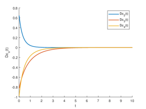
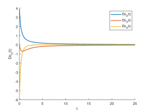
   Figure 1. (a) $\dot{c}_{n}(t)$ for $n=2,3,4$ when both $\mu_{k}(t)$ and $\nu_{k}(t)$ are M.D. (b) $\dot{c}_{n}(t)$ for $n=2,3,4$ when $\mu_{k}(t)$ is M.D. and $\nu_{k}(t)$ is M.I.

   

   

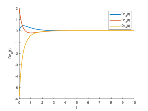
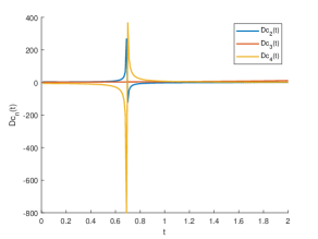
   Figure 2. (a) $\dot{c}_{n}(t)$ for $n=2,3,4$ when $\mu_{k}(t)$ is M.D. and $\nu_{k}(t)$ is Osc. (b) $\dot{c}_{n}(t)$ for $n=2,3,4$ when $\mu_{k}(t)$ is M.I. and $\nu_{k}(t)$ is M.D.

   

   

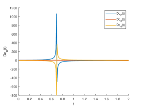
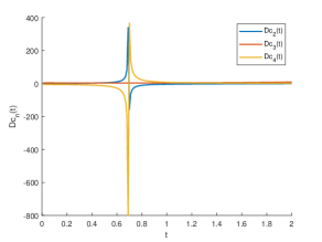
   Figure 3. (a) $\dot{c}_{n}(t)$ for $n=2,3,4$ when both $\mu_{k}(t)$ and $\nu_{k}(t)$ are M.I.  (b) $\dot{c}_{n}(t)$ for $n=2,3,4$ when $\mu_{k}(t)$ is M.I. and $\nu_{k}(t)$ is Osc.

2. When $\mu_{k}(t)$ is monotonically increasing, then for any choice of $\nu_{k}(t)$, the system for perturbed $\dot{c}_{n}(t)$ initially appears to be stable, but then experiences a sudden disturbance or perturbation that causes it to become temporarily unstable. However, the system eventually recovers from this disturbance and returns to a stable state (see Figure 2(b), Figure 3(a), and Figure 3(b)). The phenomenon is commonly known as transient instability or transient instability followed by recovery to stability [13, 19].

3. When $\mu_{k}(t)$ is oscillating and $\nu_{k}(t)$ is either monotonically decreasing or oscillating, the system for perturbed $\dot{c}_{n}(t)$ experiences instability that leads to sustained oscillations without converging to a stable state whatsoever choice of $d$ and $t$ one makes. The oscillations persist indefinitely, and the system does not return to a stable condition (see Figure 4(a) and Figure 4(b)). The phenomenon is often referred to as persistent oscillation or sustained oscillation [13, 19].

   

   

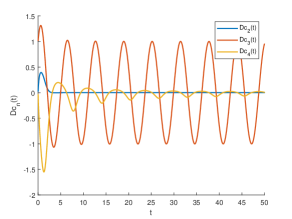
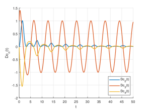
   Figure 4. (a) $\dot{c}_{n}(t)$ for $n=2,3,4$ when $\mu_{k}(t)$ is Osc. and $\nu_{k}(t)$ is M.D.  (b) $\dot{c}_{n}(t)$ for $n=2,3,4$ when both $\mu_{k}(t)$ and $\nu_{k}(t)$ are Osc.

4. For $\mu_{k}(t)$ oscillating and $\nu_{k}(t)$ monotonically increasing, the system for perturbed $\dot{c}_{n}(t)$ initially exhibits stability, but as $t$ increases, it becomes increasingly unstable, and the amplitude of oscillations grows continuously, eventually tending to infinity (see Figure 5). The phenomenon you’re describing is commonly referred to as instability with growing amplitude or exponential instability [13, 19]. This is one of the case in which the stability can be controlled by varying the parameter $d$ (upto certain $t$).

   

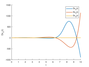
   Figure 5. $\dot{c}_{n}(t)$ for $n=2,3,4$ when $\mu_{k}(t)$ is Osc. and $\nu_{k}(t)$ is M.I.

5. When both $\mu_{k}(t)$ and $\nu_{k}(t)$ are monotonically decreasing, the system for perturbed $\dot{\lambda}_{n}(t)$ exhibits transient response where the system initially deviates from its original state but eventually stabilizes as $t$ increases (see Figure 6(b)).

   

   

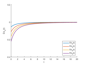
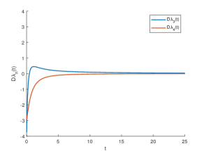
   Figure 6. (a) $\dot{\lambda}_{n}(t)$ for $n=2,3,4,5$ without any perturbation  (b) $\dot{\lambda}_{n}(t)$ for $n=3,4$ when both $\mu_{k}(t)$ and $\nu_{k}(t)$ are M.D.

   

   

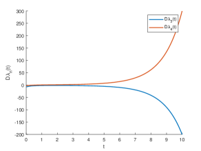
   Figure 7. (a) $\dot{\lambda}_{n}(t)$ for $n=3,4$ when $\mu_{k}(t)$ is M.D. and $\nu_{k}(t)$ is M.I.  (b) $\dot{\lambda}_{n}(t)$ for $n=3,4$ when $\mu_{k}(t)$ is M.D. and $\nu_{k}(t)$ is Osc.

   

   

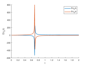
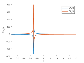
   Figure 8. (a) $\dot{\lambda}_{n}(t)$ for $n=3,4$ when $\mu_{k}(t)$ is M.I. and $\nu_{k}(t)$ is M.D.  (b) $\dot{\lambda}_{n}(t)$ for $n=3,4$ when both $\mu_{k}(t)$ and $\nu_{k}(t)$ are M.I.

   

   

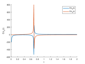
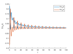
   Figure 9. (a) $\dot{\lambda}_{n}(t)$ for $n=3,4$ when $\mu_{k}(t)$ is M.I. and $\nu_{k}(t)$ is Osc.  (b) $\dot{\lambda}_{n}(t)$ for $n=3,4$ when $\mu_{k}(t)$ is Osc. and $\nu_{k}(t)$ is M.D.

   

   

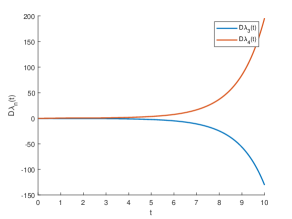
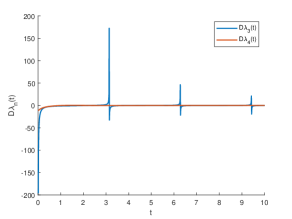
   Figure 10. (a) $\dot{\lambda}_{n}(t)$ for $n=3,4$ when $\mu_{k}(t)$ is Osc. and $\nu_{k}(t)$ is M.I.  (b) $\dot{\lambda}_{n}(t)$ for $n=3,4$ when both $\mu_{k}(t)$ and $\nu_{k}(t)$ are Osc.

6. When $\mu_{k}(t)$ is either monotonically decreasing or oscillaing but $\nu_{k}(t)$ monotonically increasing, the system for perturbed $\dot{\lambda}_{n}(t)$ remains stable for some time but then becomes unstable, but in this case, no oscillations are present (see Figure 7(a) and see Figure 10(a)), contrary to Figure 5. These are also the cases in which the stability upto certain $t$ can be controlled by varying the parameter $d$.

7. When $\mu_{k}(t)$ is either monotonically decreasing or oscillaing and $\nu_{k}(t)$ is also oscillating, the system’s (perturbed $\dot{\lambda}_{n}(t)$) behavior alternates between stable periods and episodes of instability characterized by sharp spikes or disturbances (see Figure 7(b) and see Figure 10(b)). The intermittent nature of the instability suggests that there may be periodic factors or conditions influencing the system’s dynamics, leading to the observed pattern of behavior. The phenomenon is often referred to as intermittent instability or periodic instability [13, 19].

8. When $\mu_{k}(t)$ is monotonically increasing, then for any choice of $\nu_{k}(t)$, the system for perturbed $\dot{\lambda}_{n}(t)$ exhibits transient instability [13, 19] discussed in Note 2 (see Figure 8(a), Figure 8(b), and Figure 9(a)).

9. When $\mu_{k}(t)$ is oscillaing and $\nu_{k}(t)$ is monotonically decreasing, the (perturbed $\dot{\lambda}_{n}(t)$) system’s response initially exhibits oscillatory behavior due to the disturbances, but over time, the amplitude of the oscillations decreases until the system settles into a stable state (see Figure 9(b)). The damping effect gradually reduces the magnitude of the disturbances until they no longer significantly affect the system’s behavior, allowing it to achieve stability. The phenomenon is called damped instability [13, 19].

These numerical illustrations provide the advantage of understanding the type of stability (instability) that may occur at specific values, which in turn will be useful in handling the corresponding physical system effectively. On the other hand, a strong theoretical approach needs to be developed in obtaining the range of parameters involved in the stability behaviour of the physical system given by Theorem 2.1.

References

- [1] M. J. Atia, A. Martínez-Finkelshtein, P. Martínez-González and F. Thabet, Quadratic differentials and asymptotics of Laguerre polynomials with varying complex parameters, J. Math. Anal. Appl. 416 (2014), no. 1, 52–80.
- [2] C. F. Bracciali, J. S. Silva and A. Sri Ranga, Extended relativistic Toda lattice, L-orthogonal polynomials and associated Lax pair, Acta Appl. Math. 164 (2019), 137–154.
- [3] K. Castillo, M.S. Costa, A. Sri Ranga and D.O. Veronese, A Favard type theorem for orthogonal polynomials on the unit circle from a three term recurrence formula, J. Approx. Theory 184 (2014), 146–162.
- [4] K. Castillo, F. Marcellán and J. Rivero, On co-polynomials on the real line, J. Math. Anal. Appl. 427 (2015), no. 1, 469–483.
- [5] T. S. Chihara, On co-recursive orthogonal polynomials, Proc. Amer. Math. Soc. 8 (1957), 899–905.
- [6] M. Chen and H. M. Srivastava, Existence and stability of bifurcating solution of a chemotaxis model, Proc. Amer. Math. Soc. 151 (2023), no. 11, 4735–4749.
- [7] M. S. Costa, H. M. Felix and A. Sri Ranga, Orthogonal polynomials on the unit circle and chain sequences, J. Approx. Theory 173 (2013), 14–32.
- [8] J. Coussement, A. B. J. Kuijlaars and W. Van Assche, Direct and inverse spectral transform for the relativistic Toda lattice and the connection with Laurent orthogonal polynomials, Inverse Problems 18 (2002), no. 3, 923–942.
- [9] A. Deaño, L. Morey and P. Román, Non-Abelian Toda-type equations and matrix valued orthogonal polynomials, Proc. Amer. Math. Soc. 152 (2024), no. 4, 1613–1632.
- [10] P. A. Deift, Orthogonal polynomials and random matrices: a Riemann-Hilbert approach, Courant Lecture Notes in Mathematics, 3, New York University, Courant Institute of Mathematical Sciences, New York, 1999.
- [11] I. Fernández-Irisarri and M. Mañas, Toda and Laguerre-Freud equations and tau functions for hypergeometric discrete multiple orthogonal polynomials, Anal. Math. Phys. 14 (2024), no. 2, Paper No. 30, 43 pp.
- [12] J. Dini, Sur les formes linéaires et les polynomes orthogonaux de Laguerre-Hahn, Thése de Doctorat, Université Pierre et Marie Curie, Paris, 1988.
- [13] G. F. Franklin, J. D. Powell, A. Emami-Naeini and J. D. Powell, Feedback control of dynamic systems, 4, Upper Saddle River: Prentice hall, 2002.
- [14] M. E. H. Ismail, Classical and Quantum Orthogonal Polynomials in One Variable, Encyclopedia of Mathematics and its Applications, 98, Cambridge University Press, Cambridge, 2005.
- [15] M. E. H. Ismail and D. R. Masson, Generalized orthogonality and continued fractions, J. Approx. Theory 83 (1995), no. 1, 1–40.
- [16] J.S. Kim and D. Stanton, Combinatorics of orthogonal polynomials of type , Ramanujan J., (2021)
- [17] F. Marcellán, J. S. Dehesa and A. Ronveaux, On orthogonal polynomials with perturbed recurrence relations, J. Comput. Appl. Math. 30 (1990), no. 2, 203–212.
- [18] Y. Nakamura, A new approach to numerical algorithms in terms of integrable systems, Proceedings of the International Conference on Informatics Research for Development of Knowledge Society Infrastructure (2004), pp. 194–205.
- [19] N. S. Nise, Control systems engineering, John Wiley & Sons, 2020.
- [20] V. Shukla and A. Swaminathan, Spectral transformation associated with a perturbed type recurrence relation, Bull. Malays. Math. Sci. Soc. 46 (2023), no. 5, Paper No. 169, 29 pp.
- [21] B. Simon, Orthogonal Polynomials on the Unit Circle. Part 1: Classical Theory, American Mathematical Society Colloquium Publications, 54, Part 1, American Mathematical Society, Providence, RI, 2005.
- [22] S. Malik, O. M. Lavrenteva, M. Idan and A. Nir, Controlled stabilization of rotating toroidal drops in viscous linear flow, J. Fluid Mech. 952 (2022), Paper No. A38, 22 pp.
- [23] L. Vinet and A. Zhedanov, An integrable chain and bi-orthogonal polynomials, Lett. Math. Phys. 46 (1998), no. 3, 233–245.