\begin{overpic}[width=433.62pt]{resources/teaser/teaser_v2_arxiv.png} \end{overpic}

Figure 1. Our Gaussian primitives are capable of representing complex scenes with global illumination support. This Dressing Table scene is modeled entirely by our primitives ($\sim$5.5 million primitives). It features a variety of geometric structures, ranging from hard surfaces to dense, unstructured aggregates, as well as different types of materials, such as near-specular, glossy, diffuse, and emissive. We show renders with two drastically different lighting configurations and highlight accurate effects including glossy reflections and color bleeding.

Unified Gaussian Primitives for Scene Representation and Rendering

Abstract.

Searching for a unified scene representation remains a research challenge in computer graphics. Traditional mesh-based representations are unsuitable for dense, fuzzy elements, and introduce additional complexity for filtering and differentiable rendering. Conversely, voxel-based representations struggle to model hard surfaces and suffer from intensive memory requirement. We propose a general-purpose rendering primitive based on 3D Gaussian distribution for unified scene representation, featuring versatile appearance ranging from glossy surfaces to fuzzy elements, as well as physically based scattering to enable accurate global illumination. We formulate the rendering theory for the primitive based on non-exponential transport and derive efficient rendering operations to be compatible with Monte Carlo path tracing. The new representation can be converted from different sources, including meshes and 3D Gaussian splatting, and further refined via transmittance optimization thanks to its differentiability. We demonstrate the versatility of our representation in various rendering applications such as global illumination and appearance editing, while supporting arbitrary lighting conditions by nature. Additionally, we compare our representation to existing volumetric representations, highlighting its efficiency to reproduce details.

1. Introduction

Scene representation is a fundamental building block of computer graphics. It determines the types of content that can be expressed, the compatible rendering algorithms, and ultimately influences the quality of the rendering. Throughout the development of computer graphics, numerous scene representations have been proposed, yet achieving a unified representation that reconciles both surfaces and volumes remains a challenging problem. Polygon meshes with textures are the most common representation, supported by mature hardware rendering acceleration for both rasterization and ray tracing. Meshes are well-suited for modeling connected hard surfaces but struggle to represent dense, fine elements existed in nature, such as hair, fur, grains, and foliage. Additionally, the discrete characteristic of meshes poses challenges for essential graphics applications such as level-of-detail (Vicini et al., 2021; Bako et al., 2023; Weier et al., 2023) and differentiable rendering (Zhao et al., 2020). Conversely, volumes model 3D objects as fields of microscopic scatterers, excelling at representing aggregated content but are less effective for hard surfaces. Traditionally, Volumes are discretized as (and interpolated between) voxels, which are not scalable due to high memory requirement. This often limits resolution and leads to the loss of high-frequency details. The recent success of 3D Gaussian splatting (3DGS) (Kerbl et al., 2023) suggests using anisotropic 3D Gaussian mixtures for fitting, achieving superior reconstruction quality. However, 3DGS remains an incomplete scene representation as it only records radiance fields.

The adaptability of Gaussians to complex geometry, as demonstrated by 3DGS, inspires us to develop a Gaussian-based rendering primitive not just for radiance fields, but for general-purpose light transport and appearance modeling. Crucially, we design each Gaussian to be an atomic primitive, meaning that we do not explicitly simulate volumetric random walks within it. This concept is analogous to a triangle, the primitive for mesh-based representations. This approach contrasts with defining the spatially varying extinction coefficient as a sum of Gaussians, where sub-Gaussian scattering still requires explicit tracking. To achieve this, we combine the Gaussians with a non-exponential, linear transmittance model (Vicini et al., 2021), such that the free-flight distributions of Gaussians can be disentangled. The linear transmittance model allows our primitive to adapt to both hard surfaces and aggregated elements that exhibit semi-transparency. Each Gaussian primitive can thus be assigned with its own phase function, enabling meaningful appearance modeling and authoring. Using our primitives, a scene becomes a novel kind of heterogeneous, non-exponential volume. We derive efficient Monte Carlo operations, such as free-flight distribution sampling, for the volume to be rendered by Monte Carlo path tracing with full global illumination.

Our primary goal in this work is to propose a novel unified scene representation capable of expressing rich appearance and compatible with Monte Carlo path tracing. We demonstrate the advantages of our representation via several rendering applications, including global illumination and appearance editing. Recognizing that a new representation inherently lacks data or content compared to more mature counterparts, we provide methods to convert other popular representations into our representation. Additionally, we showcase gradient-based transmittance optimization as a proof-of-concept differentiable rendering application. While our framework can potentially support an end-to-end image-based inverse rendering pipeline, this is not the focus of this work.

To summarize, our contributions include:

• A novel 3D Gaussian-based volumetric rendering primitive that can handle both hard surfaces and aggregated elements.

• Efficient Monte Carlo operations for our non-exponential heterogeneous scene representation that enables full path tracing.

• A flexible phase function that incorporates both aggregated geometric configurations and reflectance properties of each surface element.

• Various rendering applications based on our representation, including gradient-based transmittance optimization.

2. Related Work

Scene representation is a fundamental and long-standing problem in computer graphics. Our work draws inspiration from volumetric rendering, point-based graphics, and the recent advancements in 3D Gaussian-based representations. In the following, we survey key related works in these fields.

Volumetric Light Transport

Light transport simulation in participating media is based on the theory of radiative transfer (Chandrasekhar, 1960) and involves solving the radiative transfer equation (RTE). Due to its recursive nature, Monte Carlo integration is required to solve the RTE unbiasedly. Extensive studies have been conducted in compute graphics for efficient Monte Carlo techniques, and we refer readers to Novák et al. (2018) for a comprehensive review. The original RTE only models participating media consisting of isotropic, independently distributed microscopic scatterers. It is extended by the microflake theory (Jakob et al., 2010) to handle anisotropic scatterers, and by non-exponential transport (Bitterli et al., 2018; Jarabo et al., 2018) to model the spatial correlation between the scatterers. These extensions to the original RTE greatly broaden the capability of volumes to represent diverse objects, resulting in more versatile scene representations.

Volumetric Scene Representations

Using volumes to represent complex geometry has been explored extensively since first introduced by Kajiya and Kay (1989). Volumes are traditionally used to approximate the rendering of dense, unstructured geometries such as fur, hair, and foliage (Neyret, 1998; Decaudin and Neyret, 2009; Koniaris et al., 2014; Moon et al., 2008). The microflake theory has extended volumetric representations to model fabric and cloth (Zhao et al., 2011, 2012; Khungurn et al., 2015). Given that high-resolution volumes can be very memory-intensive, several works address the challenge of downsampling microflake volumes while preserving the self-shadowing effect (Zhao et al., 2016; Loubet and Neyret, 2018). In granular material rendering, explicit grain instances are switched to volumes to achieve acceleration (Moon et al., 2007; Meng et al., 2015; Müller et al., 2016; Zhang and Zhao, 2020). Non-exponential transport has inspired studies on unified representations that support both opaque surfaces and volumes (Vicini et al., 2021; Bako et al., 2023; Weier et al., 2023).

Neural Implicit Representations

The seminal work of neural radiance field (NeRF) (Mildenhall et al., 2020) has popularized implicit neural field as an effective tool for capturing 3D objects (Martel et al., 2021; Barron et al., 2022; Müller et al., 2022). Compared to traditional voxel discretization, neural fields can better reconstruct fine details, albeit with the added cost of training and extra inference. However, radiance fields only record the outgoing radiance under fixed illumination at capture time, limiting their interaction with different lighting conditions at render time. Various extensions have been proposed to predict simple material parameters and reflectance (Bi et al., 2020; Srinivasan et al., 2021; Jin et al., 2023; Boss et al., 2021a, b; Zhang et al., 2021a; Zheng et al., 2021; Lyu et al., 2022; Zhang et al., 2023; Zeng et al., 2023), but most are significantly constrained in simulating light transport and global illumination effects. Our work does not aim to solve the end-to-end inverse rendering problem. Instead, we propose a general-purpose primitive for scene representation and forward rendering. We also demonstrate its differentiability to open up possibilities for future inverse rendering applications.

Point-based Graphics

A classical family of modeling and rendering techniques use point primitives (Alexa et al., 2004; Kobbelt and Botsch, 2004). A scene is modeled by small, unstructured point-like primitives such as disks (Pfister et al., 2000) or Gaussians (Zwicker et al., 2001b, a). Rendering of point primitives involves projecting them screen space and perform proper reconstruction filtering (“splatting”) to avoid holes and aliases. More recent work explores the differentiability of point primitives for inverse rendering tasks (Yifan et al., 2019; Lassner and Zollhofer, 2021). Additionally, point primitives are used as proxy geometry or irradiance cache for real-time global illumination (Ritschel et al., 2008, 2009; Wright et al., 2022; Andreas et al., 2021).

3D Gaussian-based Representations

Recently, Kerbl et al. (2023) develop 3D Gaussian splatting (3DGS) that extends the EWA volume splatting framework (Zwicker et al., 2001a) to be differentiable and uses 3D Gaussians to optimize and render radiance fields. 3DGS achieves state-of-the-art reconstruction quality and offers significantly faster rendering speed compared to previous NeRF approaches. Since its debut, 3DGS has inspired a number of Gaussian-based representations with different focuses, such as for mesh reconstruction (Huang et al., 2024; Guédon and Lepetit, 2023), avatar rendering (Saito et al., 2023), and inverse rendering (Gao et al., 2023). While not modeling the full light transport, 3DGS demonstrates the effectiveness of anisotropic Gaussians in adapting to complex geometries, especially thin structures.

3. Preliminaries

3.1. 3D Gaussian-based Representations

A scaled 3D Gaussian distribution is defined as

(1) $$G(x;c,\mu,\Sigma)=\frac{c}{(2\pi)^{\frac{3}{2}}|\Sigma|^{\frac{1}{2}}}\exp\Big{(}-\frac{1}{2}(x-\mu)^{\mkern-1.5mu\mathsf{T}}\Sigma^{-1}(x-\mu)\Big{)},$$

where $\mu$ is the mean, $\Sigma$ is the covariance matrix, and $c$ is the magnitude. The covariance matrix can be decomposed into a rotation matrix $R$ and a scale matrix $S$:

(2) $$\Sigma=(RS)(RS)^{\mkern-1.5mu\mathsf{T}}.$$

Intuitively, $\mu$, $R$, and $S$ form an affine transform that transforms an isotropic Gaussian distribution centered at the origin to an anisotropic one centered at $\mu$.

3.2. Volumetric Light Transport

In its integral form, the radiative transfer equation (RTE) (Chandrasekhar, 1960) defines the outgoing radiance as a recursive integral over the distance a ray traveled within the volume

$$L(x,\omega)\, = \,\,\int_{0}^{b}\mathcal{P}(x,x_{t})L_{s}(x_{t},\omega)\,\mathrm{d}t+\mathcal{T}(x,x_{b})L_{b}(x_{b},\omega),$$

(3) $$L_{s}(x,\omega)\, = \,\,L_{e}(x,\omega)+\int_{\mathbb{S}^{2}}f_{p}(\omega_{i},\omega;x)L(x,\omega_{i})\mathrm{d}\omega_{i},$$

where $x_{t}=x+t\omega$, $b$ is the distance to the closest external boundary surface or infinity if none, $\mathcal{P}$ is the free-flight distribution, $\mathcal{T}$ is the transmittance function, $L_{b}$ is the external emission from either the boundary surface or free space, and $L_{s}$ is the source term. $\mathcal{P}$ and $\mathcal{T}$ are interdependent as the former is a probability distribution function (PDF), and the latter is one minus the corresponding cumulative distribution function (CDF):

$$\mathcal{T}(x,x_{t})=1-\int_{0}^{t}\mathcal{P}(x_{t^{\prime}})\mathrm{d}{t^{\prime}}\Leftrightarrow\mathcal{P}(x,x_{t})=-\frac{\partial}{\partial t}\mathcal{T}(x,x_{t}).$$

The source term $L_{s}$ consists of self-emission $L_{e}$ and the in-scattering term, which is the inner product of the phase function $f_{p}$ and the (recursive) incident radiance. Note that we have factored absorption into the phase function, similar to the formulation by Zhao et al. (2016).

Traditional volumetric representations are modeled as microscopic scatterers that are independently distributed in 3D space, leading to an exponential free-flight distribution and transmittance function:

(4) $$\mathcal{T}(x,x_{t}) =\exp\Big{(}-\int_{0}^{t}\sigma_{\mathrm{t}}(x_{t^{\prime}})\mathrm{d}{t^{\prime}}\Big{)},$$

(5) $$\mathcal{P}(x,x_{t}) =-\frac{\partial}{\partial t}\mathcal{T}(x,x_{t})=\sigma_{\mathrm{t}}(x_{t})\exp\Big{(}-\int_{0}^{t}\sigma_{\mathrm{t}}(x_{t^{\prime}})\mathrm{d}{t^{\prime}}\Big{)},$$

where $\sigma_{\mathrm{t}}$ is the spatially varying extinction coefficient, which intuitively controls the density of the volume. Note that $\mathcal{T}$ and $\mathcal{P}$ only differ by $\sigma_{\mathrm{t}}$. This is coincidentally due to the unique property of the exponential function being invariant under differentiation. Because $\mathcal{P}$ includes the nonlinear exponential function, the exponential free-flight PDF is not additive. This introduces a theoretical challenge if one attempts to define a volume as the sum of “exponential Gaussian primitives”. To see this, suppose we define the extinction coefficient of an exponential volume as $\sigma_{\mathrm{t}}(x)=\sum_{k}G_{k}(x)$. The total free-flight PDF is then different from the sum of free-flight PDFs of individual Gaussians:

(6) $$\begin{split}&\Big{(}\sum_{k}G_{k}(x_{t})\Big{)}\exp\Big{(}-\int_{0}^{t}\Big{(}\sum_{k}G_{k}(x_{t^{\prime}})\Big{)}\mathrm{d}{t^{\prime}}\Big{)}\neq\\ &\sum_{k}G_{k}(x_{t})\exp\Big{(}-\int_{0}^{t}G_{k}(x_{t^{\prime}})\mathrm{d}{t^{\prime}}\Big{)}.\end{split}$$

This implies that it is impossible to define the property of each Gaussian in isolation and “assemble” them together to form the final volume. Instead, the entire continuous volume must be treated in its entirety. Therefore, it is not suitable to define a Gaussian as a rendering primitive within the exponential formulation.

3.3. Non-exponential Transport

Non-exponential transport has been introduced to model the spatial correlation in participating media and thus enhance the expressiveness of volumetric representations (Jarabo et al., 2018; Bitterli et al., 2018; Vicini et al., 2021). In non-exponential transport, $\mathcal{T}$ and $\mathcal{P}$ are no longer required to be exponential, and thus do not share a similar form. In particular, Vicini et al. (2021) propose a transmittance function that interpolates between exponential and linear transmittance

(7) $$\mathcal{T}(x,x_{t}) =\gamma\exp(-\tau)+(1-\gamma)\max(0,1-\frac{1}{2}\tau),$$

(8) $$\tau =\int_{0}^{t}\sigma_{\mathrm{t}}(x_{t}^{\prime})\mathrm{d}{t^{\prime}},$$

where $\gamma$ is the interpolation weight. The $1/2$ factor is applied to ensure that two modes have the same mean free path. Vicini et al. (2021) have performed extensive experiments to demonstrate that the linear component reflects the negative correlation exhibited by hard surfaces. This, in turns, helps a volumetric representation to better model surface-like objects and reduce artifacts such as leaking.

4. Linear Transmittance Gaussian Primitives

Our goal is to define a general-purpose volumetric rendering primitive based on 3D Gaussian distribution. We begin by analyzing the feasibility and requirements for defining such a primitive. 3DGS has convincingly demonstrated the advantages of anisotropic 3D Gaussians for adapting to complex shapes. However, to be truly usable in light transport, we need to define how these Gaussians interact with light. This includes the attenuation of light, controlled by the free-flight distribution or transmittance, and the scattering (or absorption) of light, controlled by the appearance or phase function. For the primitives to be practically valuable in modeling and rendering applications, the following properties are desirable:

It should support hard surfaces. Just like radiance fields, this capability allows the primitive to model a much wider range of objects, instead of being limited to traditional “volume-like” objects such as clouds and smoke. Unlike radiance fields, however, exponential volumes with full light transport simulation are prone to artifacts such as leaking. To address this issue, we draw inspiration from the hybrid transmittance function by Vicini et al. (2021), as its linear component models negative correlation for hard surfaces.

Appearance should be defined on a per-primitive level. We treat primitives as the atomic elements of the scene, using appearance to abstracts away all sub-primitive scattering interactions. This decision benefits efficiency by avoiding explicit simulation of random walks inside each primitive. Additionally, since fitting any non-trivial geometry often results in many overlapping Gaussians, the appearance of overlapped regions should be well-defined for meaningful authoring and editing. As previously discussed, this is not achievable with exponential transport (Eq. 6).

To meet these properties, we propose a novel kind of heterogeneous, non-exponential volume by combining the merits of Gaussians and the linear transmittance function from Vicini et al. (2021). The transmittance and the corresponding free-flight distribution are defined as follows:

(9) $$\mathcal{T}(x,x_{t}) =\max\Big{(}0,1-\frac{1}{2}\int_{0}^{t}\Big{(}\sum_{k}G_{k}(x_{t^{\prime}})\Big{)}\mathrm{d}{t^{\prime}}\Big{)},$$

(10) $$\mathcal{P}(x,x_{t}) =-\frac{\partial}{\partial t}\mathcal{T}(x,x_{t})=\begin{cases}\frac{1}{2}\sum_{k}G_{k}(x_{t}),&\text{if }t\leq t_{\mathrm{sat}},\\ 0,&\text{otherwise},\end{cases}$$

where the saturating distance $t_{\mathrm{sat}}$ is the ray travel distance such that $\mathcal{T}(x,x_{t_{\mathrm{sat}}})=0$. Fig. 2 illustrates the above definitions in 2D flatland. It is clear from Eq. 10 that the total free-flight PDF is simply the sum of the PDFs of individual primitives. This implies that when integrating § 3.2, we can sample an individual primitive and compute its contribution separately from other primitives. In other words, the appearance of a primitive is decoupled from other overlapping primitives. The linear transmittance improves the ability to model negatively correlated hard surfaces. On the other hand, it does not compromise the ability to model objects with more stochastic characteristics such as foliage. Indeed, as we will demonstrate in § 7.2, with suitable optimization, the final heterogeneous transmittance can approach an arbitrary target.

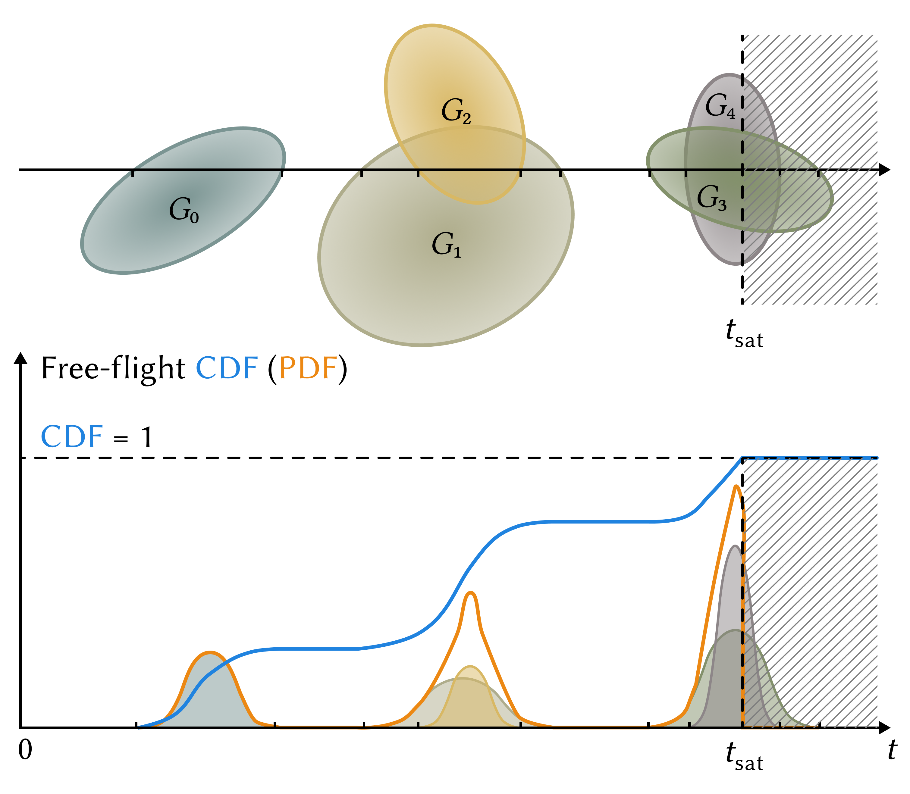
Figure 2. 2D flatland illustration of a ray traveling through a heterogeneous volume consisting of 5 Gaussian primitives (top) and the corresponding free-flight CDF and PDF (bottom). The CDF is accumulated from $0$ to $1$, where it reaches the saturating distance $t_{\mathrm{sat}}$. The ray is effectively “blocked” at this point, and the PDF is 0 afterwards.

4.1. Primitive Operations

3D Gaussians support several key operations for volumetric rendering that are either in closed forms or can be computed efficiently. These operations serve as the building blocks of our scene rendering algorithms, introduced in § 5. We further define the corresponding appearance for a Gaussian primitive in § 6. Notably, our Gaussian primitive exhibits close resemblance to how a triangle serves as the primitives in mesh-based representations.

Ray Integral

Given a ray $x_{t}=x+t\omega,t\in[t_{0},t_{1}]$ and a Gaussian primitive $G(x)$, we aim to compute the probability of the ray being scattered by the primitive. With the linear transmittance model, this is essentially the integral of $G(x)$ along $r$ from $t_{0}$ to $t_{1}$:

(11) $$I(t_{0},t_{1})=\frac{c}{(2\pi)^{\frac{3}{2}}|\Sigma|^{\frac{1}{2}}}\int_{t_{0}}^{t_{1}}\exp\Big{(}-\frac{1}{2}(x_{t}-\mu)^{\mkern-1.5mu\mathsf{T}}\Sigma^{-1}(x_{t}-\mu)\Big{)}\,\mathrm{d}{t}.$$

This integral can be solved in closed form (utilizing the error function $\mathtt{erf}$). Detailed derivation and the final expression are provided in Appendix A.

Ray Sampling

To sample along a ray that intersects a single Gaussian primitive, we can simply invert Eq. 11. The inverse error function $\mathtt{erfinv}$ is standard in mainstream numerical libraries. We then consider the case when a ray intersects multiple overlapping primitives and solve it again by CDF inversion. Given a random number $u\in[0,1)$ and a ray, we seek to find a root $t\in[t_{0},t_{1}]$ for

(12) $$u=F(t;t_{0})=\frac{1}{2}\sum_{k}I_{k}(t_{0},t).$$

Although $F(t)$ cannot be analytically inverted, we observe that $F(t)$ is non-decreasing, making the Newton-Raphson method suitable for solving Eq. 12. The derivative $\mathrm{d}F/\mathrm{d}t$ is simply the sum of the evaluations of all primitives. As will be discussed in § 5, our full algorithm can prune away most cases, making such explicit inversion rarely needed. When it is indeed required, we can always guarantee the existence of a unique solution, and provide a fairly tight initial bracket $[t_{0},t_{1}]$, such that usually only a few iterations are required for convergence. Alternatively, one could explore other analytic sampling techniques even when the CDF cannot be analytically inverted (Heitz, 2020).

Bounding Shapes

A Gaussian distribution has an infinite support in 3D space. In practice, we would like to truncate its contribution at a certain extent to give it a finite size, thereby accelerating intersection tests. We first determine the ellipsoidal isosurface where the distribution evaluates to less than a threshold of the peak:

(13) $$\frac{G(x;c,\mu,\Sigma)}{G(\mu;c,\mu,\Sigma)}=\epsilon\Leftrightarrow\Big{\lVert}\sqrt{\frac{-1}{2\ln\epsilon}}(RS)^{-1}(x-\mu)\Big{\rVert}=1,$$

where we utilize Eq. 2. Here, $\epsilon$ is usually set to $0.01$, and any contribution outside the ellipsoid is discarded. We can further calculate the bounding box of the ellipsoid to be used by intersection acceleration structures.

5. Scene Traversal and Rendering Operations

Similar to Monte Carlo rendering of exponential volumes, to efficiently solve § 3.2 in a heterogeneous scene composed of our Gaussian primitives, a Monte Carlo renderer needs to support two core operations: sampling the free-flight distribution and evaluating the transmittance. As both operations involve traversing the scene along a ray, we utilize the bounding shapes of primitives to build a kd-tree acceleration structure. In the following, we describe efficient techniques for both operations using the kd-tree. Specifically, our sampling technique relies on the non-overlapping spatial subdivision by the kd-tree, which is why we do not use a bounding volume hierarchy that can produce overlapping nodes.

5.1. Free-flight Distribution Sampling

Given a ray $x_{t}=x+t\omega,t\in[t_{0},t_{1}]$, and a random number $u\in[0,1)$, traditional Monte Carlo volumetric rendering usually performs free-flight distance sampling, where the goal is to generate random samples of ray travel distances $t$ such that $t\nolinebreak\sim\nolinebreak\mathcal{P}(x,x_{t})$. Distinctively, we aim at sampling discrete primitives $k$ such that $k\nolinebreak\sim\nolinebreak I_{k}(t_{0},t_{1})$. We do not need to determine the exact scattering locations inside the primitives.

We achieve this by inverting the heterogeneous CDF of Eq. 10, as illustrated in Fig. 3a. Thanks to the linear transmittance model, this is straightforward for the most part because $\mathcal{P}$ is “almost” a linear sum of all involved primitives. We traverse the scene along the ray, accumulate the CDF contributed by each visited primitive, and check if the sum reaches $u$. If so, we return the last visited primitive as the sample. If the CDF never reaches $u$, the ray reaches free space, and thus we sample the background. In fact, Eq. 10 implies that it is not necessary to traverse the primitives in any specific order as long as the traversal does not exceed the saturating distance. This is in contrast with exponential volumes where the free-flight PDF is order-dependent.

However, there is a catch that lies in the nonlinearity of $\mathcal{P}$ caused by the clamping at the saturating distance $t_{\mathrm{sat}}$. If multiple primitives touch the saturating boundary $t=t_{\mathrm{sat}}$, we call them ambiguous. This situation is illustrated in Fig. 3b. In this case, inverting the free-flight CDF by accumulating those primitives one by one results in bias. To understand this situation, let $M\coloneq\{m_{1},...,m_{q}\}$ be the set of ambiguous primitives in the order of traversal. Let $C_{\mathrm{prev}}$ be the accumulated CDF prior to visiting $M$, and $t_{\mathrm{prev}}$ be the travel distance so far. There exists a particular primitive $m_{i}$ such that

$$C_{\mathrm{prev}}+\frac{1}{2}\sum_{j=1}^{i-1}I_{m_{j}}(t_{\mathrm{prev}},t_{\mathrm{sat}})<1\leq C_{\mathrm{prev}}+\frac{1}{2}\sum_{j=1}^{i}I_{m_{j}}(t_{\mathrm{prev}},t_{\mathrm{sat}}).$$

It is clear that CDF inversion by sequential accumulation will only consider $\{m_{1},...,m_{i}\}$ and discard $\{m_{i+1},...,m_{q}\}$, thus incorrectly skewing the free-flight distribution. The correct way to disambiguate them, illustrated in Fig. 3c, is to first perform ray sampling by Eq. 12 to find the exact distance $t_{u}$ such that

(14) $$C_{\mathrm{prev}}+\int_{t_{\mathrm{prev}}}^{t_{u}}\mathcal{P}(x,x_{t})\mathrm{d}{t}=u.$$

Then, we sample the $j$-th primitive in $M$ proportional to $I_{j}(t_{\mathrm{prev}},t_{u})$. The disambiguation step is not always required for every sampling operation, as it may have already finished before visiting any ambiguous primitive. In fact, it is required at most once for each sampling operation.

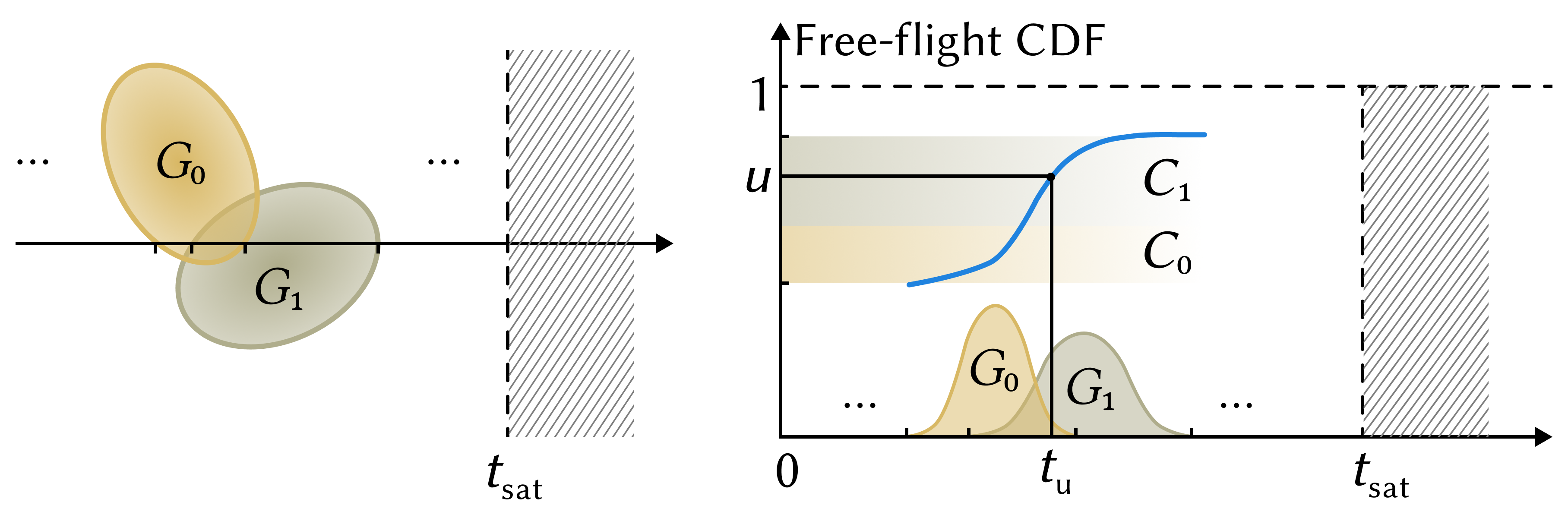
(a)

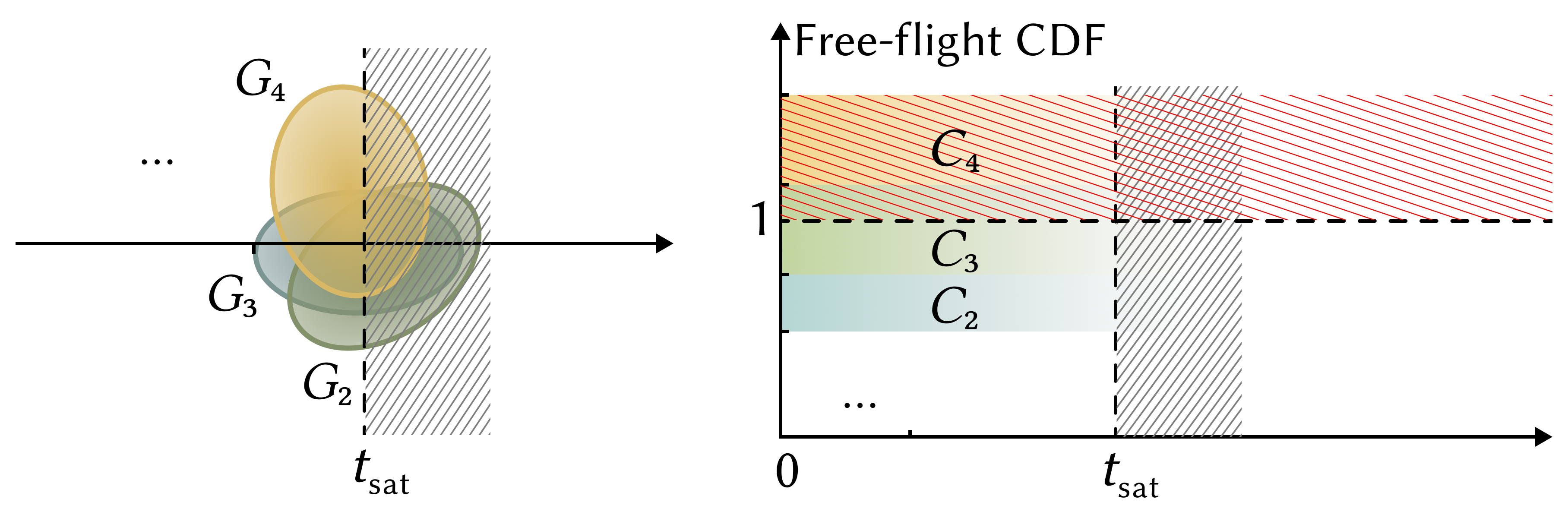
(b)

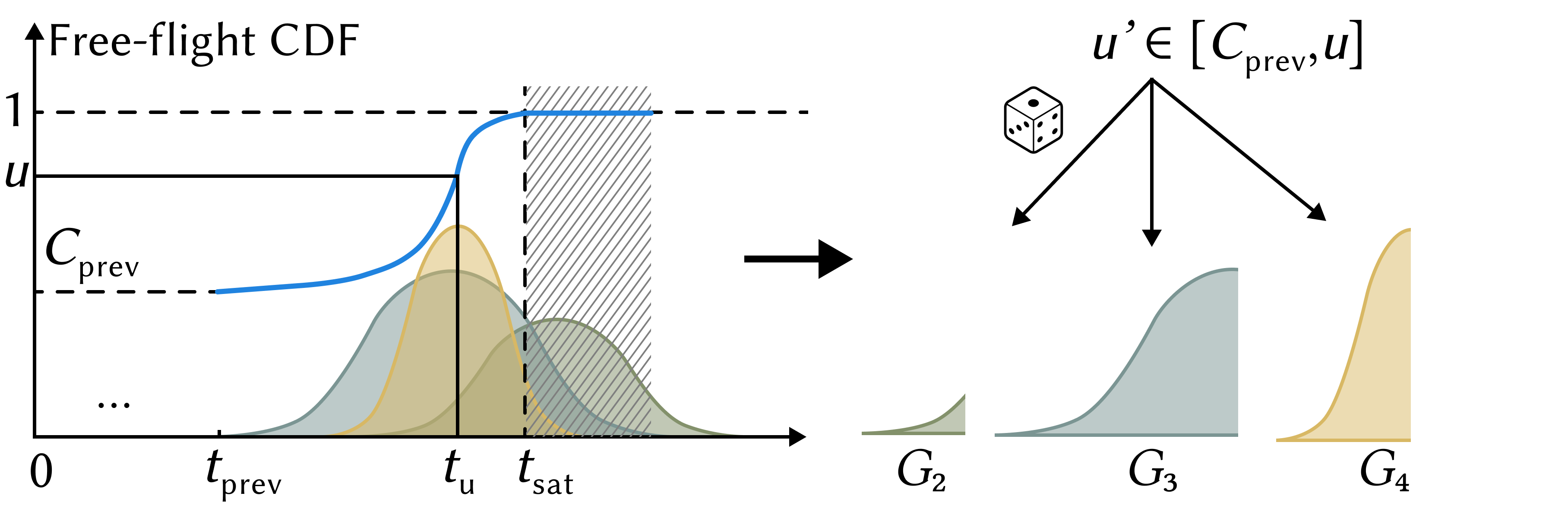
(c)

Figure 3. Illustration for free-flight distribution sampling. (a) If the primitives do not touch $t=t_{\mathrm{sat}}$, it is safe to invert the free-flight CDF by accumulating the per-primitive contributions and check the interval $u$ falls within. Overlapped primitives are automatically handled. (b) However, when primitives are ambiguous, doing so will skew the free-flight distribution. Here, $G_{4}$ will never be sampled. (c) Instead, we need to perform a disambiguation step by first solving for $t_{u}$ and then re-sample the primitives based on the clamped distributions.

In the full sampling algorithm, a ray traverses the scene using the kd-tree to prune non-intersecting primitives while keeping track of the accumulated CDF. At each interior node, we recursively visit its front and back children. This establishes an implicit front-to-back order without explicit sorting, which is necessary even if our free-flight PDF is order-independent because we need to avoid tracing behind $t_{\mathrm{sat}}$. At each leaf node, there are several possible cases:

1. There is only one primitive. In this case, it does not matter whether it is ambiguous or not, and we simply perform per-primitive CDF accumulation.

2. There are multiple non-ambiguous primitives. We perform per-primitive CDF accumulation for each primitive.

3. There are multiple ambiguous primitives. We need to perform a disambiguation step.

Case (3) can be further optimized by partitioning the leaf node into sub-node segments that consist of different subsets of the primitives in the node, as illustrated in Fig. 4. We can then repeat the above classification on a per-segment level and only an ambiguous segment requires a disambiguation step. This further simplifies the convergence of ray sampling. The partition uses the Bentley-Ottmann line sweeping algorithm (O’Rourke, 1998). We provide pseudocode for our free-flight distribution sampling in § 5.1. The algorithm only requires 2 random numbers and is thus friendly to stratification. Fig. 5 validates the convergence of rendering using the algorithm.

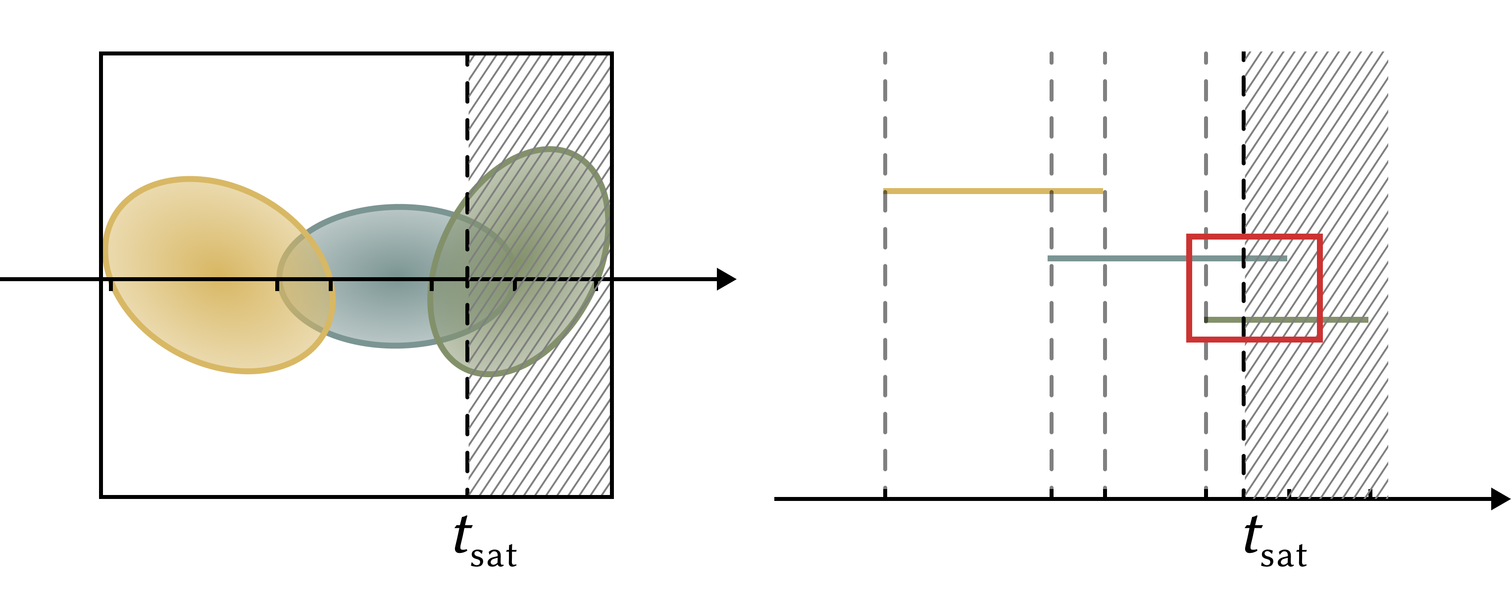
Figure 4. Even when there are multiple primitives in a leaf node, it is possible that not all of them are ambiguous. We use line sweeping to find the exact ambiguous segment (highlighted by the red box).

1 spp	16 spp	256 spp	Reference

Figure 5. Rendering 1K random Gaussians assigned with random colors using our free-flight sampling algorithm with different samples per pixel (spp). Difference images against the reference are provided.

5.2. Transmittance Evaluation

The transmittance evaluation is much more straightforward compared to free-flight distribution sampling. We simply traverse the scene and decrease the transmittance by each visited primitive until it either reaches 0 or we exit the traversal. We also employ Russian roulette for efficiency trade-off. The pseudocode for transmittance evaluation is in § 5.2.

6. Appearance

The linear transmittance model ensures that the probability of a ray scattered by each Gaussian primitive is simply additive. It allows us to conveniently define the appearance of each primitive individually. In this work, we define appearance models at the primitive level, conceptually abstracting away all sub-primitive scattering interactions. This design decision eliminates the need to explicit simulate random walks inside each primitive, thereby making rendering more efficient.

A Gaussian primitive can simply be a part of a flat surface, or represents a collection of small surface elements with different orientations. Therefore, a useful appearance model for the primitive should incorporate this aggregated effect while still being compatible with simple flat scenarios. Inspired by the microflake theory (Jakob et al., 2010; Heitz et al., 2015), we describe the orientations by a normal distribution function (NDF) $D(n)$ and its visible normal distribution function (VNDF) $D_{\omega_{o}}(n)$ when conditioned by a viewing direction $\omega_{o}$:

(15) $$\begin{split}D_{\omega_{o}}(n)&=\frac{1}{\sigma(\omega_{o})}D(n)\langle n\cdot\omega_{o}\rangle,\\ \sigma(\omega_{o})&=\int_{\mathbb{S}^{2}}D(n)\langle n\cdot\omega_{o}\rangle\,\mathrm{d}{n},\end{split}$$

where $\sigma(\omega)$ is the projected area that serves as the normalization term for $D_{\omega_{o}}(n)$, and $\langle\cdot\rangle$ is the clamped dot product. The appearance of a Gaussian primitive is affected by both the VNDF and the (cosine-weighted) base surface BSDF $f(\omega_{i},\omega_{o};n)$ that describes each oriented surface element. Formally, it is defined as a phase function which is an inner product of the VNDF and the base surface BSDF:

(16) $$f_{p}(\omega_{i},\omega_{o})=\int_{\mathbb{S}^{2}}D_{\omega_{o}}(n)f(\omega_{i},\omega_{o};n)\,\mathrm{d}{n}.$$

In the case when the primitive only models a single flat surface, $D(n)$ becomes a delta distribution, and $f_{p}$ falls back to the usual surface BSDF multiplied by the foreshortening term. Even if the base BSDF is strictly defined for a surface, the overall phase function could represent flexible geometric configurations from being surface-like to fiber-like, as illustrated in Fig. 6. We use the SGGX distribution for the (V)NDF due to its expressiveness and simplicity to evaluate, importance sample, and fit (Heitz et al., 2015).

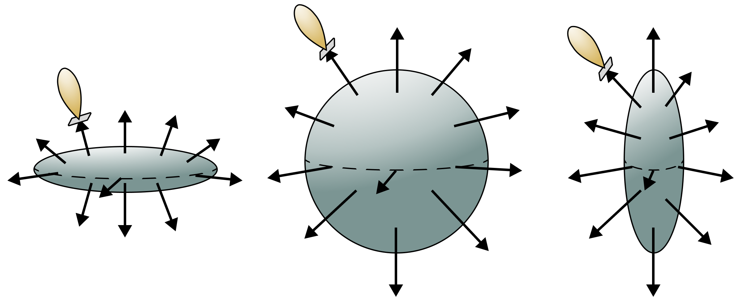
Figure 6. The phase function incorporates the underlying geometric configuration by modulating the base BSDF (yellow) with the (V)NDF (green). It can thus represent a collection of oriented surface elements that overall behaves like a surface (left), isotropic scatterer (middle), or fiber (right).

The base surface BSDF can be arbitrary valid BSDF with standard evaluation and importance sampling procedures. In this work, we primarily work with the Disney principled BSDF (Burley, 2015) due to its capability to model a wide range of materials. The Disney principled BSDF mainly consists of a microfacet specular component and a diffuse component with empirical retroflection. We refer readers to Burley (2015) for the full definition.

For our phase function to be compatible with a Monte Carlo renderer, it must support several operations, namely evaluation (evaluate Eq. 16 given $\omega_{i}$ and $\omega_{o}$), importance sampling (sample a suitable $\omega_{i}$ given $\omega_{o}$), and preferably PDF evaluation (of the importance sampling procedure) for multiple importance sampling (MIS). In the following, we describe those operations in details.

Evaluation

The integral in Eq. 16 cannot be evaluated in closed form for most non-trivial base BSDFs (one exception is perfect specular reflection). For Lambertian base BSDF, Heitz et al. (2015) suggest a simple Monte Carlo estimator by sampling the VNDF. We propose an improvement by utilizing the existing sampling routine for the base BSDF and applying an internal multiple importance sampling (MIS) between VNDF sampling and base BSDF sampling. Specifically for the Disney BSDF which is a linear combination of multiple components, we estimate each component by MIS to achieve even greater variance reduction. For its specular component, we reverse the input and output of the microfacet distribution sampling (Walter et al., 2007), generating normal $n$ given half vector $\omega_{h}$. For its diffuse component, we again similarly use cosine-weighted hemisphere sampling to generating normal $n$ given $\omega_{i}$. The pseudocode for our improved stochastic evaluation is in § 6.

Importance Sampling

We follow the original importance sampling strategy by (Heitz et al., 2015). Given a view direction $\omega_{o}$, we first sample the VNDF to generate a sample $n$. We then sample an incident direction $\omega_{i}$ using the existing strategy of the base BSDF. Since the VNDF sampling for SGGX is perfect, the sample weight is simply that of the base BSDF sampling.

Multiple Importance Sampling

It is desirable to be able to compute the PDF from the importance sampling so that the renderer can apply useful variance reduction techniques, such as MIS between light sampling and phase function sampling for next-event estimation (not to be confused with the internal MIS for the stochastic evaluation). However, the PDF follows a similar form to Eq. 16 and also cannot be computed in closed form:

(17) $$\mathrm{pdf}_{f_{p}}(\omega_{i}|\omega_{o})=\int_{\mathbb{S}^{2}}D_{\omega_{o}}(n)\mathrm{pdf}_{f}(\omega_{i}|\omega_{o};n)\,\mathrm{d}{n},$$

where $\mathrm{pdf}_{f}$ is the PDF from the base BSDF sampling technique. Moreover, a stochastic estimator for the PDF is not useful because the MIS weight requires the reciprocal of the PDF, and expectation does not commute with division (Heitz et al., 2016; Zeltner et al., 2020; Qin et al., 2015). Fortunately, MIS does not require an exact PDF to work correctly, thus we provide a simple approximation to Eq. 17 for this purpose. The approximate PDF uses a roughened SGGX for the specular component and a cosine-weighted hemisphere for the diffuse component, both parameterized by half vector. Please refer to Appendix B for details.

		Smooth Gold			Rough Copper			Plastic
Delta Surface
Surface-like
Isotropic
Fiber-like
	Naïve	Improved	Improved + MIS	Naïve	Improved	Improved + MIS	Naïve	Improved	Improved + MIS

Figure 7. Equal-sample rendering comparison of different phase function configurations with varying NDFs (rows) and base BSDFs (columns). Our improved stochastic evaluation (“Improved”) is much more efficient than the simple stochastic evaluation based on SGGX VNDF sampling only (“Naïve”). Combining it with MIS (“Improved + MIS”) provides further variance reduction. All images are rendered using 64 samples per pixel.

7. Data Acquisition

In this section, we describe methods to acquire data from other synthetic source data for our representations. As previously mentioned, our work focuses on defining a unified scene representation with our Gaussian primitive and does not attempt to solve the image-based inverse rendering problem. Therefore, in order to acquire full scene data for rendering, we propose conversion processes from meshes and 3DGS data, two widely adopted existing representations.

7.1. Conversion from Existing Representations

Conversion from Meshes

We provide a heuristic method to convert a mesh to a set of Gaussian primitives. This method generates flat, opaque ellipse-like primitives to cover the original surface. We uniformly sample points on the mesh to initialize flat Gaussians aligned to the mesh surface. Let $A$ be the surface area of the mesh, $N$ be the number of Gaussians, and $(s_{x},s_{y},s_{z})$ be the diagonal elements of the rotation matrix $S$ Eq. 2. We set $s_{x}$ and $s_{y}$ to $\epsilon kA/n$, where $\epsilon$ is the cutoff threshold Eq. 13, and $k$ is an adjustable parameter set to $16$ for our experiments. $s_{z}$ is then set to $0.1s_{x}$.

After initializing the shape parameters, we determine the appearance counterpart for each Gaussian by assigning those parameters from the source mesh. We consider the spatial neighborhood of each Gaussian while heuristically reject outliers to better maintain the original silhouette and texture details (if textured). We generate $2048$ samples $\{p_{i}\}$ according to the Gaussian distribution and project them to the plane defined by the center $\mu$ and normal. For each $p_{i}$, we query the nearest point on the mesh and gather its BSDF parameter vector $\phi_{i}$, normal $n_{i}$, and the distance $d_{i}$ between $p_{i}$ and the returned query. We examine the similarity between a sample and the center point $\mu$ based on those attributes, following the heuristic formula

(18) $$o_{i}=\left(\bigvee\limits_{k}\|\phi_{i,k}-\phi_{\mu,k}\|>\epsilon_{k}\right)\lor\left(n_{i}\cdot n_{\mu}<1-\epsilon_{n}\right)\lor\left(d_{i}>\epsilon_{d}\right),$$

where $\phi_{*,k}$ is each BSDF parameter and $\epsilon_{*}$ are the thresholds for different attributes. If $o_{i}$ is true, the sample is rejected as an outlier. We use the distance between the closest outlier $p^{\prime}$ and $\mu$ to be $s_{x}$, and set the corresponding eigenvector $R_{x}$ as the direction from $\mu$ to $p^{\prime}$. The last eigenvector follows as $R_{y}=n_{\mu}\times\ R_{x}$. $s_{y}$ is clamped to the maximum distance such that the bounding ellipsoid of the Gaussian does not contain any outlier sample points. Finally, we average $\phi_{i}$ across the accepted samples to obtain the BSDF parameters for the primitive. The Gaussian primitives produced from this method are different from those by the concurrent work by Huang et al. (2024), which are pure 2D surfel-like surface-only representations. Their method focuses on reconstruction and does not support full appearance (weakly direction-dependent SH colors only) or further light transport. Our representation is not limited to flat Gaussians, as can be seen in the following.

(a) Mesh wireframe	(b) Point samples
(c) Render	(d) Shrunken Gaussians

Figure 8. Our heuristic method sample points from the original mesh and generates flat, opaque Gaussians to cover the mesh surface. We visualize the generated Gaussians by shrinking them (d).

Conversion from 3DGS

3DGS can optimize radiance fields using anisotropic Gaussians that adapt to complex shapes. While radiance fields cannot be directly used as input for our framework, we find 3DGS a viable tool for the initial conversion of synthetic models that include dense and thin elements, where the previous heuristic conversion method is not suitable. We generate a synthetic dataset for the model by rendering it from multiple views, which is used as the input for 3DGS. We then extract the shape parameters $\mu,R$, and $S$ for our primitives. Interestingly, there exists a mapping between the opacity $\alpha$ in 3DGS and our magnitude $c$, which we detail in Appendix C. We use this remapping to initialize our magnitudes, and further optimize transmittance as detailed in § 7.2. For each primitive, we then perform similar sampling according to the Gaussian distribution. Each sample is projected to the closest point on the original model to query normal and BSDF parameters. We obtain the phase function by averaging the BSDF parameters and fitting the SGGX NDF according to the procedure by Heitz et al. (2015). While a full image-based inverse rendering pipeline is out of scope in this work, we demonstrate the differentiation capability of our representation in § 7.2. Additionally, developing digital content creation tools for our representation, similar to those for mesh modeling and signed distance field sculpting (Adobe, 2024), would be a desirable future direction.

7.2. Transmittance Optimization

For differentiable rendering, our Gaussian primitive benefits from not requiring dedicated techniques to handle the discontinuities in the rendering integral (Zhao et al., 2020), as it maintains continuity similar to other volumetric representations. To demonstrate the usefulness of our primitive’s differentiability, we develop a proof-of-concept system that optimizes the transmittance of our models. Thanks to its simple formulation, differentiating our linear transmittance model is considerably simpler than the traditional exponential model or the hybrid model by Vicini et al. (2021). Given a ray, the accumulated free-flight CDF (one minus transmittance) is a simple sum of the free-flight probabilities from each primitive:

(19) $$C=\sum_{k=1}^{n}I_{k}(t^{-}_{k},t^{+}_{k}),$$

where each primitive intersects the ray from $t^{-}_{k}$ to $t^{+}_{k}$. Let $\phi_{k}$ be a parameter of the $k$-th primitive, partial derivatives of $C$ w.r.t. $\phi_{k}$ is trivially

(20) $$\frac{\partial C}{\partial\phi_{k}}=\frac{\partial I_{k}(t^{-}_{k},t^{+}_{k})}{\partial\phi_{k}}.$$

The right term can be effectively computed by applying automatic differentiation (AD) to Eq. 11. Strictly speaking, $C$ should be less or equal to 1, but we relax its definition during the optimization. The case when $C>1$ is analogous to a ray penetrating multiple layers of surfaces. We currently do not apply any special handling to this case, but it could be interesting to consider improvements to better handle objects with complex interior structure.

A model is initially converted by either method discussed above, and its transmittance is then refined to better match that of the source asset. We render transmittance images and compute the L2 loss across multiple views. We trace one ray for each pixel with jittered sub-pixel offsets to compute and differentiate transmittance according to Eq. 19 and Eq. 20. We use forward AD to compute the analytic parameter gradients of each primitive, and backward AD to propagate the loss to each primitive. Doing so reduces the overhead caused by a pure backward AD implementation (Kerbl et al., 2023). We optimize this loss over all parameters of all Gaussian primitives using the Adam optimizer (Kingma and Ba, 2014) with a learning rate of $210-5$ for rotation and $110-4$ for all other parameters. After each iteration, scales and magnitudes are clamped to be positive, and rotations are re-normalized.

In Fig. 9, we apply the transmittance optimization to two models initialized by 3DGS. The Plant model has 220K primitives, while the Tall Vase model has 799K primitives. Both models are optimized for 50 iterations using 8 views at 512$\times$512 resolution. Both models consist of long, thin branches that are not captured by 3DGS faithfully, but can be recovered quickly by our post optimization. In addition, our optimization also improves the silhouette of the spokes of the Tall Vase. Overall improvement in transmittance can be verified by the loss curves. The process take 16 and 26 minutes, respectively (see § 8 for machine specifications).

		Plant			Tall Vase
Render
Transmittance
Tr. Loss
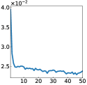
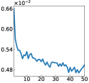
	Original / loss curve	Initial	Iter. 50	Original / loss curve	Initial	Iter. 50

Figure 9. Applying transmittance optimization to Gaussian models initialized from 3DGS. We visualize the transmittance (from a selected view) of each model before and after the optimization, and compare it to that of the original model. Transmittance losses and loss curves are provided. We encourage readers to zoom in to better identify the differences.

8. Applications and Results

In this section, we present rendering results and various applications using our Gaussian primitives. We also provide a supplemental video that includes rendering sequences with camera and light animations. We implement our framework in a custom CPU renderer. All results are generated on a desktop computer with an Intel® Core™ i9-13900K CPU, as well as a workstation with an AMD Ryzen™ Threadripper™ PRO 3995WX CPU. Timings of all renders are provided in Table 1. Typically, the majority ($\sim$85%) of rendering time is spent on kd-tree traversal, bounding ellipsoid intersection test, and ray integral evaluation. The disambiguation step in § 5.1 takes less than 5% of time. Note that we choose to implement our method in an offline fashion path tracer to demonstrate the full capability of our representation. We refrain from practical techniques such as path reuse, temporal accumulation, or denoising to avoid artifacts such as correlated patterns, ghosting, bias, and overblurring. As listed in Table 1, our performance falls into a typical range from minutes to hours for scenes containing 100K-5.8M, using up to 4K samples per pixel (spp). primitives.

Table 1. Rendering specifications and timings. Orange timings are measured on the AMD CPU, and blue timings are measured on the Intel CPU.

Figure	#Prim.	Res.	Spp	Bounce	Time
Fig. 1	5.5M	2000$\times$1200	4096	8	2h 22m
Fig. 10, Dragon	500K	1280$\times$720	2048	2	2m 10s
Fig. 10, Blanket	131K	1280$\times$720	2048	2	10m 56s
Fig. 12, Garden	5.8M	1920$\times$1080	2048	2	4h 20m
Fig. 12, Stump	4.9M	1920$\times$1080	2048	2	4h 50m
Fig. 11, Color Tree	750K	1024$\times$1024	256	1	5m 16s
Fig. 11, Plant	220K	1024$\times$1024	256	1	2m 16s

Complex Scene Rendering with Global Illumination

In Fig. 1, we demonstrate the versatility of our Gaussian primitive to represent objects with a wide range of geometric and material characteristics. The Dressing Table scene is modeled entirely by our primitives and contains parts that are acquired in different ways. The room, table, dragon, and logo are converted from meshes, while the plants, candle set, and blanket are converted from 3DGS reconstruction. Additionally, several objects, such as the mirror and neon light bars, are modeled analytically. Our Gaussian primitives can adapt to different shapes, including flat surfaces and thin fibers, thanks to their anisotropic definition. The volumetric formulation naturally handles semi-transparency for dense, stochastic details.

The scene also features a variety of materials that include near-specular, glossy, and diffuse, demonstrating the expressiveness of our appearance definition. The phase function of our primitive incorporates the effect of base BSDF and NDF, thus allowing it to aggregate the appearance caused by many differently oriented small elements, such as the plants. Meanwhile, for flat surfaces like the floor and table, it naturally reverts to the familiar surface BSDF formulation. Thanks to our improved stochastic evaluation scheme and the approximated PDF for MIS (Fig. 7), the variance contributed by phase functions is low and diminishes quickly as more samples are used by the path tracing integrator.

Crucially, our framework supports full unbiased global illumination with Monte Carlo (volumetric) path tracing. This is in contrast to rasterization approaches including 3DGS, and volumetric ray marching approaches such as NeRF. Both families of approaches are fundamentally limited to the first few dimensions of the path space, and are simply incapable of solving the infinite dimensional light transport integral. Fig. 1 includes two renders with drastically different lighting setups. In the “daylight” setup, the scene is lit by an area light and an environment light; in the “night” setup, the scene is lit by a logo, neon light bars, and candles, all modeled as emissive Gaussian primitives. The number of emissive primitives exceeds 10K combined. Both renders showcase various global illumination effects including soft shadows, color bleeding, and inter-reflection. Additional sequences with zoomed-in camera animations are provided in the supplemental video.

Appearance Editing

One of the goals of this work is to make the Gaussian primitive useful for general 3D content authoring. Our representation is volumetric and thus does not require UV parameterization, which is naturally supported by meshes. Instead, we seek a more general method for texturing 3D objects without the need for UV mapping. To this end, we extend UV-less texturing techniques for our representation. Fig. 10 demonstrates two example techniques on different models. The first technique, which we term extended triplanar mapping, generalizes the well-known triplanar mapping for surfaces. The traditional triplanar mapping projects a shading point to three axis-aligned planes, performs texture sampling on the planes, and blend the three samples based on the surface normal. We can naturally generalize this for our representation by instead blending based on the projected area of the SGGX NDF $\sigma(\omega)=\sqrt{\omega^{\mkern-1.5mu\mathsf{T}}S\omega}$, where $S$ is the SGGX matrix (Heitz et al., 2015). Moreover, we can edit the NDF itself by applying the extended triplanar mapping with a normal map. This is achieved by defining the blended normal in the coordinate space formed by the SGGX eigenvectors, and rotating the dominant SGGX eigenvector to it. The second row of Fig. 10 shows the texturing results using the extended triplanar mapping, including both base BSDF and NDF editing to produce the bumpy effect.

Alternatively, we may apply 3D procedural noises to our representation just like other volumetric representations. In the third row of Fig. 10, we use procedural phasor noise (Tricard et al., 2019) to modulate the base color, roughness, and metallic parameters of our models to create patterns.

	Dragon		Blanket
Unmodified
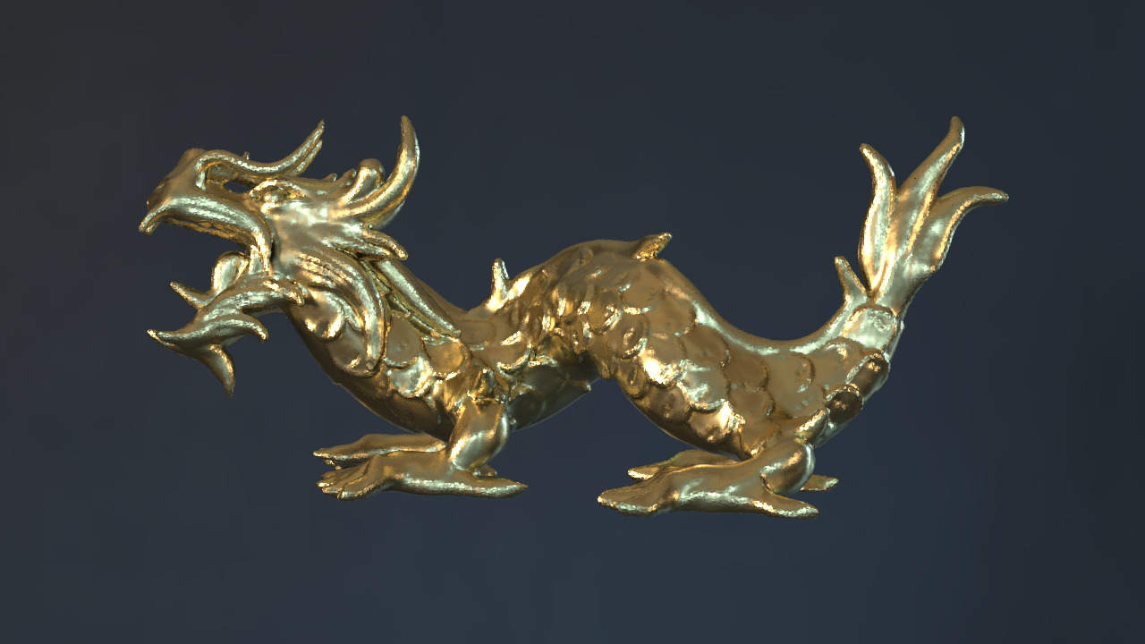
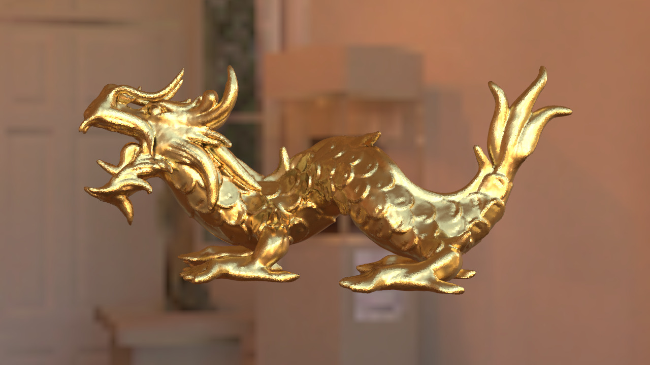
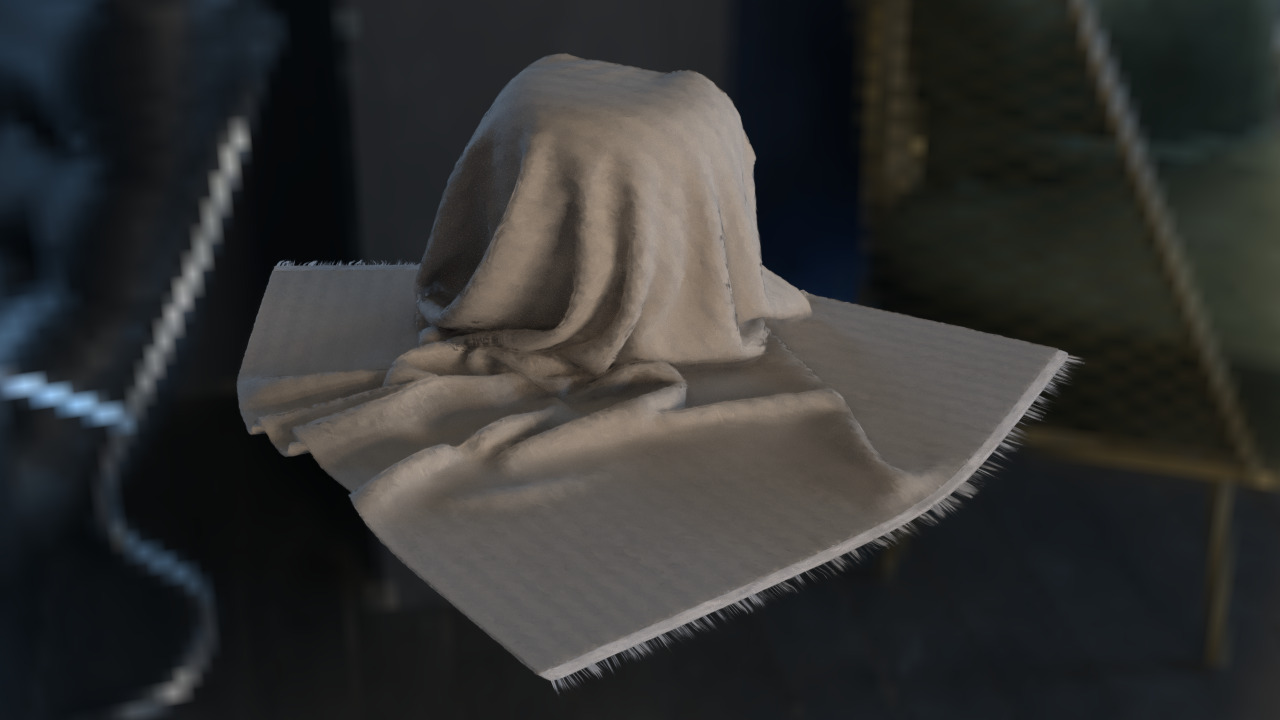
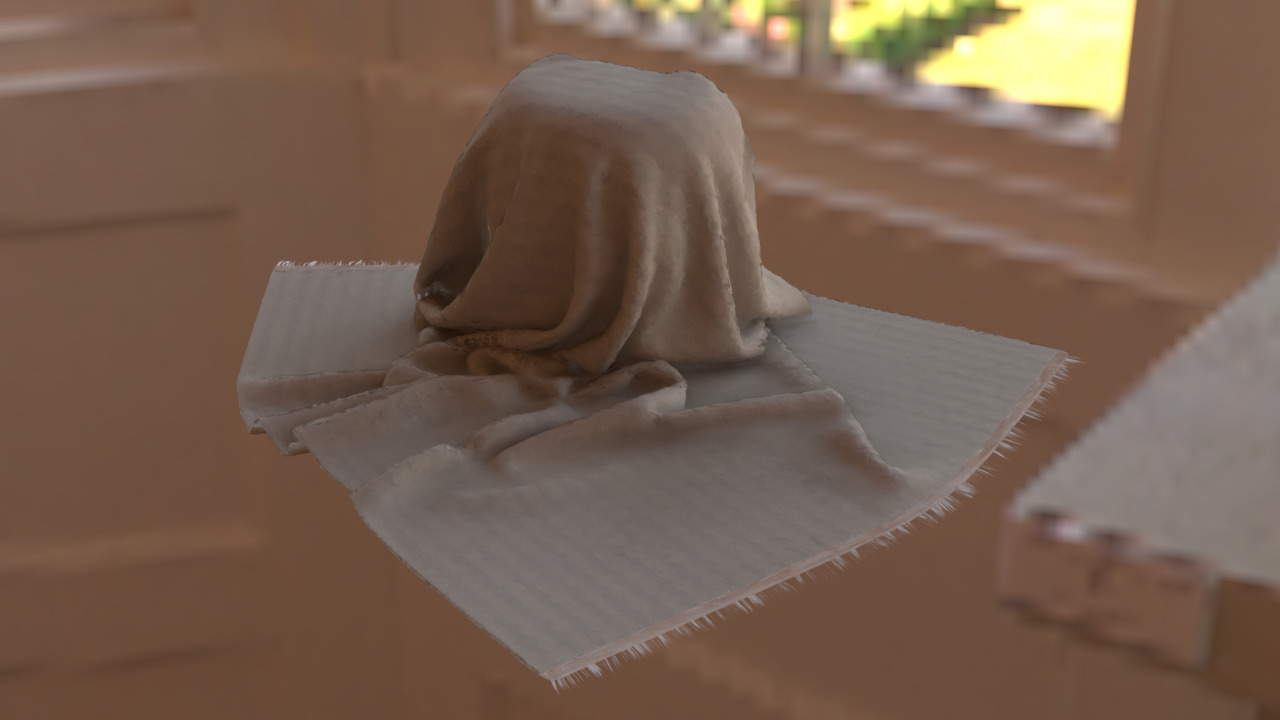
Ext. triplanar
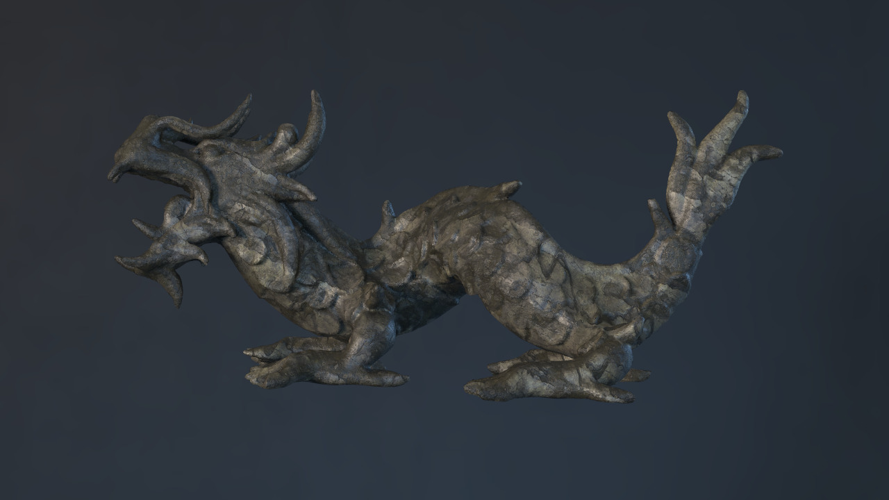
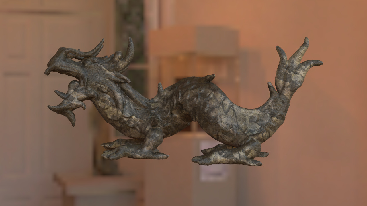
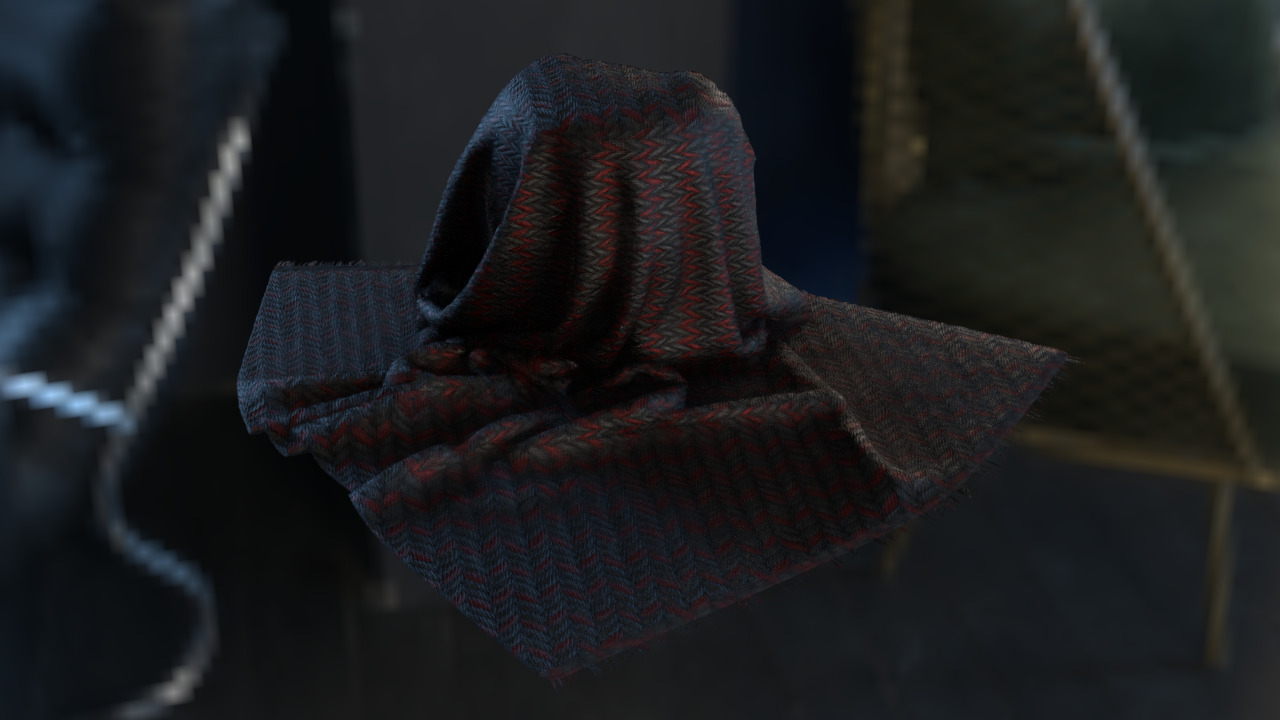
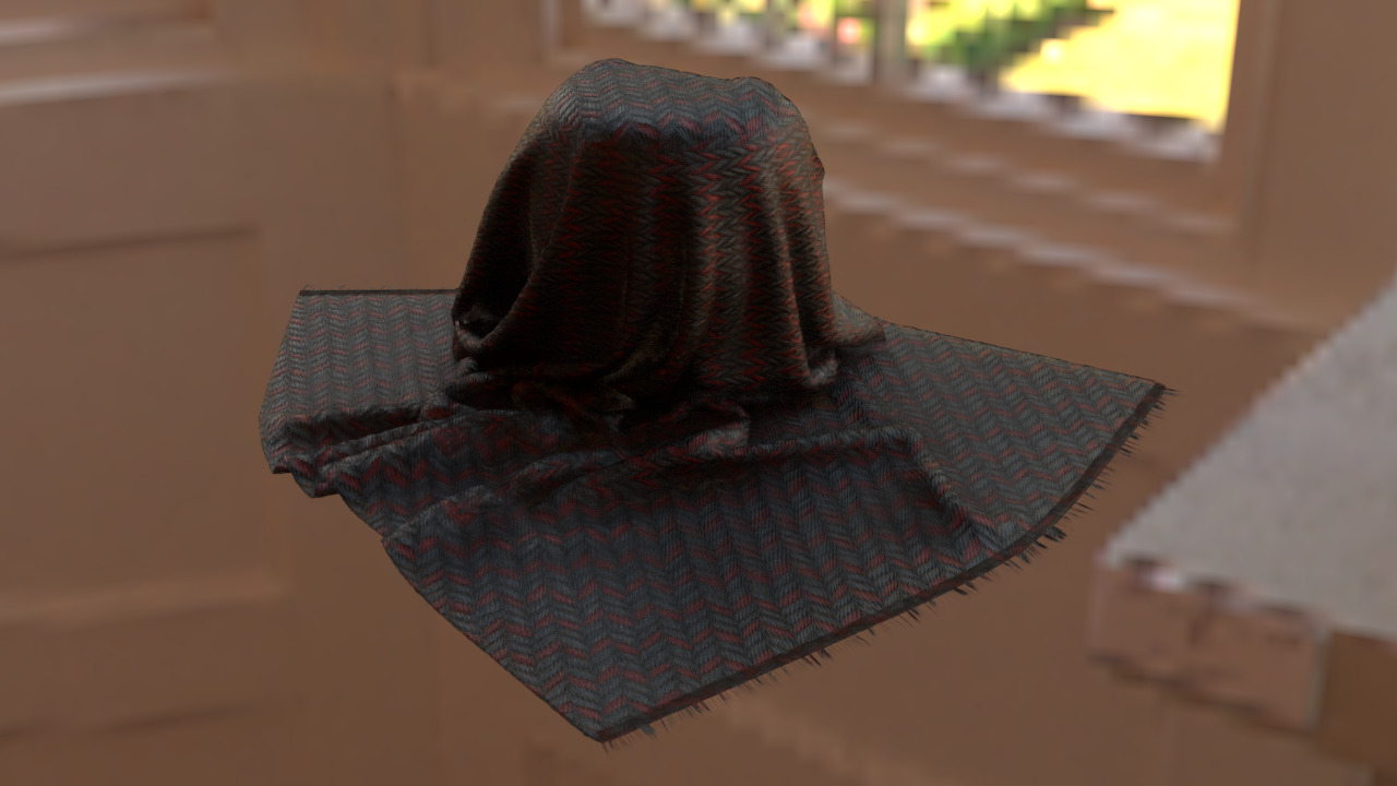
Procedural
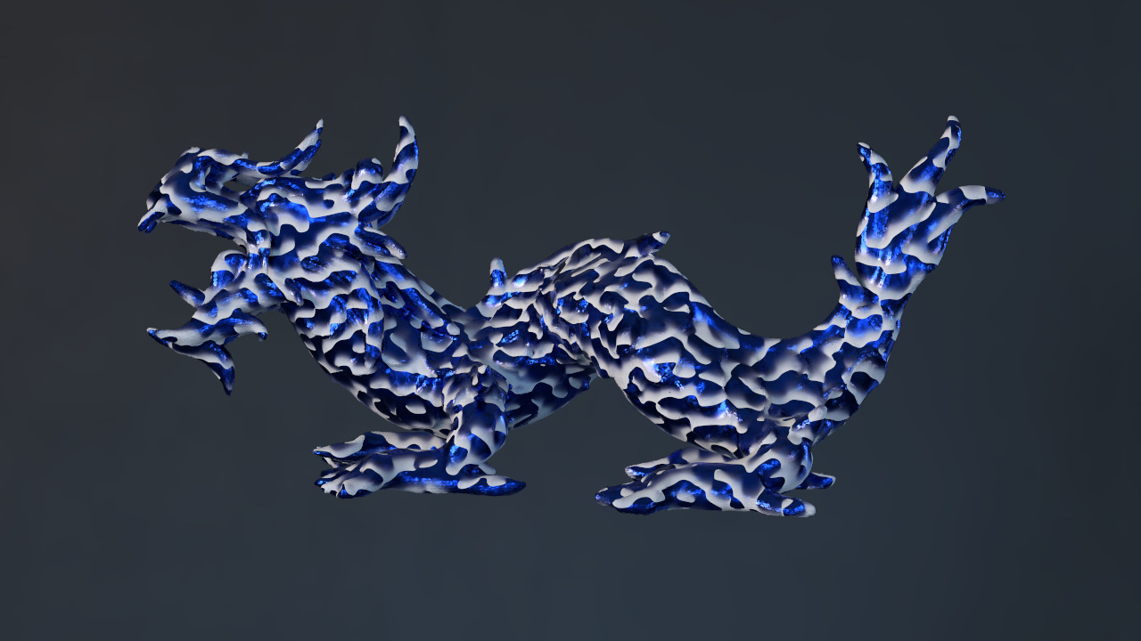
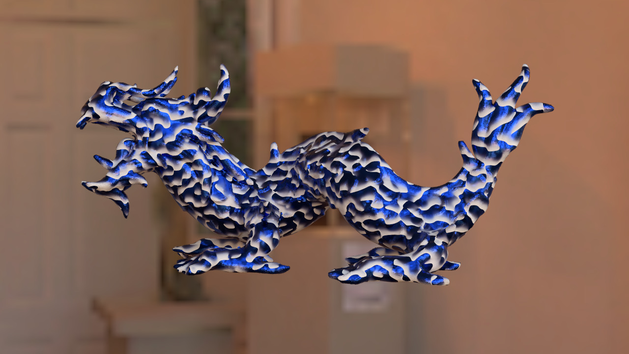
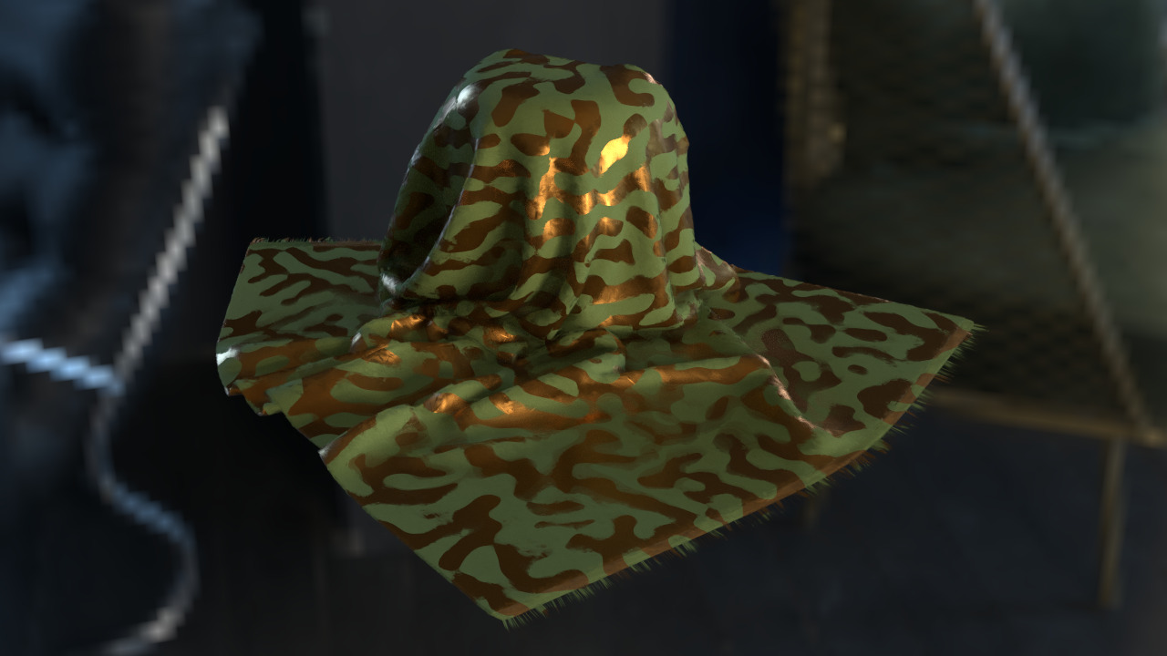
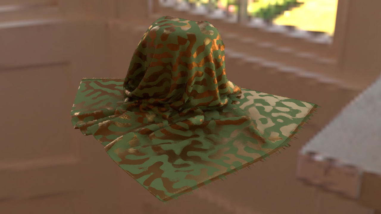
	Lighting 1	Lighting 2	Lighting 1	Lighting 2

Figure 10. Editing the appearance of our models by different techniques. Both the base BSDF and the NDF (second row) can be altered to produce visually interesting effects.

Comparison to Voxel-based Representation

In Fig. 11, we compare our representation to the traditional volume representation consisting of regular voxels. We perform a simple voxelization of our models by resampling the free-flight PDF. For each voxel, we evaluate all overlapping Gaussians at the voxel center. The phase function parameters are similarly resampled. The voxel grid is then linearly interpolated and rendered by ray marching. We evaluate the reconstruction quality using different voxel resolutions. Even using 8$\times$ more voxels than the number of Gaussians, the reconstruction quality is still significantly more inferior. This is expected because unlike Gaussian mixtures that can approximate signals at arbitrary frequency, regular grid sampling is limited by the Nyquist-Shannon sampling theorem and the resolution must be at least twice the signal bandwidth to avoid aliasing. It would require an impractical amount of storage to properly represent the thin structures common in vegetation. Conversely, Gaussian primitives are much more effective at capturing fine geometry details.

	Color Tree			Plant
Eq. num voxels	8$\times$ num voxels	Gaussians ($\sim$750K)	Eq. num voxels	8$\times$ num voxels	Gaussians ($\sim$220K)

Figure 11. Comparison between Gaussian models and voxelized models in different resolutions. Gaussian primitives are much more effective at representing sharp, detailed structure than voxels. Note that our current simple voxelization causes self-shadowing that leads to slight darkening. Direct illumination only.

Re-rendering the Original 3DGS Scenes

The original 3DGS scenes are radiance fields and therefore cannot simulate light transport. Nonetheless, we demonstrate compatibility by performing an empirical conversion as described in § 7. The converted scenes can then be rendered under arbitrary lighting conditions, as demonstrated in Fig. 12. Both the Garden and the Stump scenes are rendered with new area lights and environment lights, producing plausible lighting and soft shadows. Additional rendering sequences are provided in the supplemental video.

Garden	Stump
\begin{overpic}[width=216.81pt]{resources/gs_lit/garden_original.jpg} \end{overpic}	\begin{overpic}[width=216.81pt]{resources/gs_lit/stump_original.jpg} \end{overpic}
(a) Original
\begin{overpic}[width=216.81pt]{resources/gs_lit/garden_1.jpg} \end{overpic}	\begin{overpic}[width=216.81pt]{resources/gs_lit/stump_1.jpg} \end{overpic}
(b) Lighting 1
\begin{overpic}[width=216.81pt]{resources/gs_lit/garden_2.jpg} \end{overpic}	\begin{overpic}[width=216.81pt]{resources/gs_lit/stump_2.jpg} \end{overpic}
(c) Lighting 2

Figure 12. 3DGS scenes ((a)) empirically converted into our representation and rendered with different lighting conditions ((b) and (c)). Note the soft shadows introduced by the new light sources that are not present in the original radiance fields.

9. Conclusion

In this work, we have presented a novel volumetric rendering primitive for unified scene representation. By combining anisotropic 3D Gaussian distribution and a non-exponential, linear transmittance model, our primitives can adapt to hard surfaces, thin structures, and aggregated elements. The primitive appearance is defined by a flexible phase function that incorporates both the NDF of an aggregation and the base BSDF of each aggregated element. Our representation provides efficient Monte Carlo operations to enable Monte Carlo path tracing for global illumination. We have demonstrated the generality and quality of our representation with various rendering applications and provided methods to acquire data from other existing representation. Furthermore, we have implemented gradient-based transmittance optimization to showcase the simplicity of differentiating our representations, exhibiting potential for further differentiable rendering tasks.

Our method has several limitations that could serve as fruitful topics for future research. Our transmittance model shares the common limitation with the model by Vicini et al. (2021) that it does not conform to certain physical constraints, such as the weak reciprocity proposed by d’Eon (2018). Developing a reciprocal formulation for general heterogeneous non-exponential transport remains an open problem. Additionally, our phase function currently does not support refraction. Rendering refraction requires tracking the change of index of refraction when a ray enters or exits a medium boundary. When a scene is entirely modeled by our volumetric Gaussian primitives, there is no clear definition of medium boundaries and mechanism to separate interior and exterior parts. It would also be desirable to further extend our phase function to support advanced effects such as subsurface scattering. While out of scope in this work, a full path-space differentiable rendering formulation for our representation, similar to that for exponential volumes (Zhang et al., 2021b), will enable more powerful inverse rendering applications. Finally, a GPU implementation of our method will likely achieve significant performance improvement over our current CPU implementation.

Overall, we believe our work provides novel contributions toward a practical unified scene representation that encompasses both surfaces and volumes. Such unification could offer benefits to both forward and inverse rendering techniques, as well as numerous downstream graphics applications.

Appendix A Ray Integral Derivation

Without loss of generality, assume $\mu=0$. Expanding the integral term in Eq. 11 gives us

$$\int_{t_{0}}^{t_{1}}G(x_{t})\,\mathrm{d}{t} =\int_{t_{0}}^{t_{1}}\exp(-\frac{1}{2}\,x_{t}^{\mkern-1.5mu\mathsf{T}}\Sigma^{-1}x_{t})\,\mathrm{d}{t}$$

$$=\int_{t_{0}}^{t_{1}}\exp(-\frac{1}{2}\,(x+t\omega)^{\mkern-1.5mu\mathsf{T}}\Sigma^{-1}(x+t\omega))\,\mathrm{d}{t}$$

$$=\int_{t_{0}}^{t_{1}}\exp(-\frac{1}{2}\,(At^{2}+Bt+C))\,\mathrm{d}{t}$$

$$=\int_{t_{0}}^{t_{1}}\exp\Big{(}-\frac{1}{2}((A(t+\frac{B}{2A}))^{2}+(C-\frac{B^{2}}{4A}))\Big{)}\,\mathrm{d}{t}$$

$$=\exp(\frac{B^{2}}{8A}-\frac{C}{2})\int_{t_{0}}^{t_{1}}\exp(-(\sqrt{\frac{A}{2}}t+\frac{B}{2\sqrt{2A}})^{2})\,\mathrm{d}{t},$$

$$A =\omega^{\mkern-1.5mu\mathsf{T}}\Sigma^{-1}\omega,$$

$$B =\omega^{\mkern-1.5mu\mathsf{T}}\Sigma^{-1}x+x^{\mkern-1.5mu\mathsf{T}}\Sigma^{-1}\omega,$$

(21) $$C =x^{\mkern-1.5mu\mathsf{T}}\Sigma^{-1}x.$$

To continue, Let $\tau=\sqrt{A/2}\,t+B/(2\sqrt{2A})$ and perform a change of variable:

$$\int_{t_{0}}^{t_{1}}\exp(-(\sqrt{\frac{A}{2}}t+\frac{B}{2\sqrt{2A}})^{2})\,\mathrm{d}{t}=\sqrt{\frac{2}{A}}\int_{\tau_{0}}^{\tau_{1}}\exp(-\tau^{2})\,\mathrm{d}{\tau}$$

(22) $$=\sqrt{\frac{\pi}{2A}}\Big{(}\operatorname{erf}(\sqrt{\frac{A}{2}}t_{1}+\frac{B}{2\sqrt{2A}})-\operatorname{erf}(\sqrt{\frac{A}{2}}t_{0}+\frac{B}{2\sqrt{2A}})\Big{)}.$$

The final expression can then be obtained by substituting Appendix A and Appendix A into Eq. 11. If the ray is infinite ($t_{0}=-\infty$ and $t_{1}=\infty$), then Appendix A simply evaluates to $\sqrt{2\pi/A}$.

Appendix B MIS PDF Approximation

For the specular component of the Disney BSDF, the standard sampling procedure is to sample a half vector is from the VNDF of the microfacet distribution (Heitz, 2018). We approximate the overall PDF by a roughened SGGX VNDF:

$$\int_{\mathbb{S}^{2}}D_{\omega_{o}}(n)\mathrm{pdf}_{\mathrm{spec}}(\omega_{i}|\omega_{o};n)\,\mathrm{d}{n}$$

$$= \int_{\mathbb{S}^{2}}D_{\omega_{o}}(n)\frac{D_{m}(n\cdot\omega_{h})G_{1}(n\cdot\omega_{o})\langle\omega_{h}\cdot\omega_{o}\rangle}{|n\cdot\omega_{o}|}\,\mathrm{d}{n}$$

$$\approx \int_{\mathbb{S}^{2}}D_{\omega_{o}}(n)D_{m}(n\cdot\omega_{h})\,\mathrm{d}{n}$$

(23) $$\approx \;\tilde{D}_{\omega_{o}}(\omega_{h}),$$

where we first drop the low-frequency components ($G_{1}(n\cdot\omega_{o})$, $\langle\omega_{h}\cdot\omega_{o}\rangle$, and $|n\cdot\omega_{o}|$). We then utilize the fact that a SGGX distribution is equivalent to a double-sided GGX (Heitz et al., 2015). Therefore, the remaining integral becomes similar to a convolution between two SGGXs, which we further approximate by a roughened SGGX VNDF. Let $(\sigma_{1}^{2},\sigma_{2}^{2},\sigma_{3}^{2})$ be the eigenvalues of original SGGX sorted in ascending order, and $\alpha$ be the isotropic roughness of the microfacet GGX distribution. The roughened SGGX has the adjusted eigenvalues $(\sigma_{1}^{2}+\alpha^{2}\sigma_{3}^{2},\sigma_{2}^{2}+\alpha^{2}\sigma_{3}^{2},\sigma_{3}^{2})$ and the same eigenvectors as the original one.

For the diffuse component of the Disney BSDF, the standard sampling procedure is usually just cosine-weighted hemisphere sampling. We simply approximate the overall PDF as a cosine-weighted hemisphere of the half vector:

(24) $$\int_{\mathbb{S}^{2}}D_{\omega_{o}}(n)\mathrm{pdf}_{\mathrm{diff}}(\omega_{i}|\omega_{o};n)\,\mathrm{d}{n}\approx\frac{1}{\pi}\langle\omega_{h}\cdot\omega_{o}\rangle.$$

We then combine both components (with optional weighting by metallic and base color luminance) to get the overall approximation to Eq. 17. The approximate PDF admittedly lowers the effectiveness of MIS compared to the exact PDF, but overall still provides great variance reduction compared to not having MIS at all.

Appendix C Magnitude Remapping from 3DGS

3DGS renders a Gaussian by projecting it to the 2D screen space and evaluating the PDF of the projected 2D Gaussian. This is in fact similar to our ray integral for an infinite ray. To see it, consider an infinite ray with origin $x$ and direction $\omega$. Let $(u,v,\omega)$ be an orthonormal basis. The local-to-world transform is

$$M=\begin{pmatrix}R&x\\ \bm{0}&\bm{1}\end{pmatrix},\quad R=(u,v,\omega).$$

Following Zwicker et al. (2001a), the parameters of the projected 2D Gaussian are

$$\hat{\mu} =(M^{-1}\mu)_{2\times 2},$$

$$\hat{\Sigma} =(R^{-1}\Sigma R)_{2\times 2},$$

where $(\cdot)_{2\times 2}$ denotes taking the $2\times 2$ submatrix by deleting the third row and the third column. The projected 2D Gaussian is then evaluated without normalization, and multiplied by the opacity $\alpha$ as the weight in the blending process:

$$I_{\mathrm{3DGS}}=\alpha\exp\Big{(}-\frac{1}{2}\hat{\mu}^{\mkern-1.5mu\mathsf{T}}\hat{\Sigma}^{-1}\hat{\mu}\Big{)}.$$

Mathematically, evaluating the PDF of the normalized projected 2D Gaussian equals to integrating the original 3D Gaussian over an infinite ray defined by $x$ and $\omega$:

$$\frac{1}{2\pi|\hat{\Sigma}|^{\frac{1}{2}}}\exp\Big{(}-\frac{1}{2}\hat{\mu}^{\mkern-1.5mu\mathsf{T}}\hat{\Sigma}^{-1}\hat{\mu}\Big{)}=$$

$$\frac{1}{(2\pi)^{\frac{3}{2}}|\Sigma|^{\frac{1}{2}}}\int_{t_{0}}^{t_{1}}\exp\Big{(}-\frac{1}{2}(x_{t}-\mu)^{\mkern-1.5mu\mathsf{T}}\Sigma^{-1}(x_{t}-\mu)\Big{)}\,\mathrm{d}{t}.$$

Therefore, it is easy to see that by letting

(25) $$c=2\pi|\hat{\Sigma}|^{\frac{1}{2}}\alpha,$$

our infinite ray integral (Eq. 11) equals to the above blending weight used by 3DGS

$$I(-\infty,\infty)=I_{\mathrm{3DGS}}.$$

References

- (1)
- Adobe (2024) Adobe. 2024. Substance 3D Modeler. https://www.adobe.com/products/substance3d/apps/modeler.html
- Alexa et al. (2004) Marc Alexa, Markus Gross, Mark Pauly, Hanspeter Pfister, Marc Stamminger, and Matthias Zwicker. 2004. Point-based computer graphics. In ACM SIGGRAPH 2004 Course Notes. 7–es.
- Andreas et al. (2021) Brinck Andreas, Bei Xiangshun, Halén Henrik, and Hayward Kyle. 2021. Global illumination based on surfels. Advances in Real-Time Rendering in Games, SIGGRAPH Courses 1, 10.1145 (2021).
- Bako et al. (2023) Steve Bako, Pradeep Sen, and Anton Kaplanyan. 2023. Deep Appearance Prefiltering. ACM Trans. Graph. 42, 2 (2023), 23:1–23:23. https://doi.org/10.1145/3570327
- Barron et al. (2022) Jonathan T Barron, Ben Mildenhall, Dor Verbin, Pratul P Srinivasan, and Peter Hedman. 2022. Mip-nerf 360: Unbounded anti-aliased neural radiance fields. In Proceedings of the IEEE/CVF Conference on Computer Vision and Pattern Recognition. 5470–5479.
- Bi et al. (2020) Sai Bi, Zexiang Xu, Pratul Srinivasan, Ben Mildenhall, Kalyan Sunkavalli, Miloš Hašan, Yannick Hold-Geoffroy, David Kriegman, and Ravi Ramamoorthi. 2020. Neural reflectance fields for appearance acquisition. arXiv preprint arXiv:2008.03824 (2020).
- Bitterli et al. (2018) Benedikt Bitterli, Srinath Ravichandran, Thomas Müller, Magnus Wrenninge, Jan Novák, Steve Marschner, and Wojciech Jarosz. 2018. A radiative transfer framework for non-exponential media. (2018).
- Boss et al. (2021a) Mark Boss, Raphael Braun, Varun Jampani, Jonathan T Barron, Ce Liu, and Hendrik Lensch. 2021a. Nerd: Neural reflectance decomposition from image collections. In Proceedings of the IEEE/CVF International Conference on Computer Vision. 12684–12694.
- Boss et al. (2021b) Mark Boss, Varun Jampani, Raphael Braun, Ce Liu, Jonathan Barron, and Hendrik Lensch. 2021b. Neural-pil: Neural pre-integrated lighting for reflectance decomposition. Advances in Neural Information Processing Systems 34 (2021), 10691–10704.
- Burley (2015) Brent Burley. 2015. Extending the Disney BRDF to a BSDF with integrated subsurface scattering. SIGGRAPH Course: Physically Based Shading in Theory and Practice. ACM, New York, NY 19, 7 (2015), 9.
- Chandrasekhar (1960) Subrahmanyan Chandrasekhar. 1960. Radiative transfer. New York: Dover (1960).
- Decaudin and Neyret (2009) Philippe Decaudin and Fabrice Neyret. 2009. Volumetric billboards. In Computer Graphics Forum, Vol. 28. Wiley Online Library, 2079–2089.
- d’Eon (2018) Eugene d’Eon. 2018. A reciprocal formulation of nonexponential radiative transfer. 1: Sketch and motivation. Journal of Computational and Theoretical Transport 47, 1-3 (2018), 84–115.
- Gao et al. (2023) Jian Gao, Chun Gu, Youtian Lin, Hao Zhu, Xun Cao, Li Zhang, and Yao Yao. 2023. Relightable 3d gaussian: Real-time point cloud relighting with brdf decomposition and ray tracing. arXiv preprint arXiv:2311.16043 (2023).
- Guédon and Lepetit (2023) Antoine Guédon and Vincent Lepetit. 2023. Sugar: Surface-aligned gaussian splatting for efficient 3d mesh reconstruction and high-quality mesh rendering. arXiv preprint arXiv:2311.12775 (2023).
- Heitz (2018) Eric Heitz. 2018. Sampling the ggx distribution of visible normals. Journal of Computer Graphics Techniques (JCGT) 7, 4 (2018), 1–13.
- Heitz (2020) Eric Heitz. 2020. Can’t Invert the CDF? The Triangle-Cut Parameterization of the Region under the Curve. In Computer Graphics Forum, Vol. 39. Wiley Online Library, 121–132.
- Heitz et al. (2015) Eric Heitz, Jonathan Dupuy, Cyril Crassin, and Carsten Dachsbacher. 2015. The SGGX microflake distribution. ACM Transactions on Graphics (TOG) 34, 4 (2015), 1–11.
- Heitz et al. (2016) Eric Heitz, Johannes Hanika, Eugene d’Eon, and Carsten Dachsbacher. 2016. Multiple-scattering microfacet BSDFs with the Smith model. ACM Transactions on Graphics (TOG) 35, 4 (2016), 1–14.
- Huang et al. (2024) Binbin Huang, Zehao Yu, Anpei Chen, Andreas Geiger, and Shenghua Gao. 2024. 2D Gaussian Splatting for Geometrically Accurate Radiance Fields. SIGGRAPH (2024).
- Jakob et al. (2010) Wenzel Jakob, Adam Arbree, Jonathan T Moon, Kavita Bala, and Steve Marschner. 2010. A radiative transfer framework for rendering materials with anisotropic structure. In ACM SIGGRAPH 2010 papers. 1–13.
- Jarabo et al. (2018) Adrian Jarabo, Carlos Aliaga, and Diego Gutierrez. 2018. A radiative transfer framework for spatially-correlated materials. ACM Transactions on Graphics (TOG) 37, 4 (2018), 1–13.
- Jin et al. (2023) Haian Jin, Isabella Liu, Peijia Xu, Xiaoshuai Zhang, Songfang Han, Sai Bi, Xiaowei Zhou, Zexiang Xu, and Hao Su. 2023. TensoIR: Tensorial Inverse Rendering. In Proceedings of the IEEE/CVF Conference on Computer Vision and Pattern Recognition. 165–174.
- Kajiya and Kay (1989) James T. Kajiya and Timothy L. Kay. 1989. Rendering fur with three dimensional textures. ACM Trans. Graph. (1989), 271–280. https://doi.org/10.1145/74333.74361
- Kerbl et al. (2023) Bernhard Kerbl, Georgios Kopanas, Thomas Leimkühler, and George Drettakis. 2023. 3D Gaussian Splatting for Real-Time Radiance Field Rendering. ACM Transactions on Graphics 42, 4 (2023).
- Khungurn et al. (2015) Pramook Khungurn, Daniel Schroeder, Shuang Zhao, Kavita Bala, and Steve Marschner. 2015. Matching Real Fabrics with Micro-Appearance Models. ACM Trans. Graph. 35, 1 (2015), 1–1.
- Kingma and Ba (2014) Diederik P Kingma and Jimmy Ba. 2014. Adam: A method for stochastic optimization. arXiv preprint arXiv:1412.6980 (2014).
- Kobbelt and Botsch (2004) Leif Kobbelt and Mario Botsch. 2004. A survey of point-based techniques in computer graphics. Computers & Graphics 28, 6 (2004), 801–814.
- Koniaris et al. (2014) Charalampos Koniaris, Darren Cosker, Xiaosong Yang, and Kenny Mitchell. 2014. Survey of texture mapping techniques for representing and rendering volumetric mesostructure. Journal of Computer Graphics Techniques (2014).
- Lassner and Zollhofer (2021) Christoph Lassner and Michael Zollhofer. 2021. Pulsar: Efficient sphere-based neural rendering. In Proceedings of the IEEE/CVF Conference on Computer Vision and Pattern Recognition. 1440–1449.
- Loubet and Neyret (2018) Guillaume Loubet and Fabrice Neyret. 2018. A new microflake model with microscopic self-shadowing for accurate volume downsampling. Comput. Graph. Forum 37, 2, 111–121. https://doi.org/10.1111/cgf.13346
- Lyu et al. (2022) Linjie Lyu, Ayush Tewari, Thomas Leimkühler, Marc Habermann, and Christian Theobalt. 2022. Neural radiance transfer fields for relightable novel-view synthesis with global illumination. In European Conference on Computer Vision. Springer, 153–169.
- Martel et al. (2021) Julien NP Martel, David B Lindell, Connor Z Lin, Eric R Chan, Marco Monteiro, and Gordon Wetzstein. 2021. Acorn: Adaptive coordinate networks for neural scene representation. arXiv preprint arXiv:2105.02788 (2021).
- Meng et al. (2015) Johannes Meng, Marios Papas, Ralf Habel, Carsten Dachsbacher, Steve Marschner, Markus H. Gross, and Wojciech Jarosz. 2015. Multi-scale modeling and rendering of granular materials. ACM Trans. Graph. 34, 4 (2015), 49:1–49:13. https://doi.org/10.1145/2766949
- Mildenhall et al. (2020) Ben Mildenhall, Pratul P. Srinivasan, Matthew Tancik, Jonathan T. Barron, Ravi Ramamoorthi, and Ren Ng. 2020. NeRF: Representing Scenes as Neural Radiance Fields for View Synthesis. In ECCV.
- Moon et al. (2008) Jonathan T. Moon, Bruce Walter, and Steve Marschner. 2008. Efficient multiple scattering in hair using spherical harmonics. Vol. 27. 31. https://doi.org/10.1145/1360612.1360630
- Moon et al. (2007) Jonathan T Moon, Bruce Walter, and Stephen R Marschner. 2007. Rendering discrete random media using precomputed scattering solutions. In Proceedings of the 18th Eurographics conference on Rendering Techniques. 231–242.
- Müller et al. (2022) Thomas Müller, Alex Evans, Christoph Schied, and Alexander Keller. 2022. Instant neural graphics primitives with a multiresolution hash encoding. ACM Transactions on Graphics (ToG) 41, 4 (2022), 1–15.
- Müller et al. (2016) Thomas Müller, Marios Papas, Markus H. Gross, Wojciech Jarosz, and Jan Novák. 2016. Efficient rendering of heterogeneous polydisperse granular media. ACM Trans. Graph. 35, 6 (2016), 168:1–168:14. https://doi.org/10.1145/2980179.2982429
- Neyret (1998) Fabrice Neyret. 1998. Modeling, Animating, and Rendering Complex Scenes Using Volumetric Textures. IEEE Trans. Vis. Comput. Graph. 4, 1 (1998), 55–70. https://doi.org/10.1109/2945.675652
- Novák et al. (2018) Jan Novák, Iliyan Georgiev, Johannes Hanika, and Wojciech Jarosz. 2018. Monte Carlo methods for volumetric light transport simulation. In Computer graphics forum, Vol. 37. Wiley Online Library, 551–576.
- O’Rourke (1998) Joseph O’Rourke. 1998. Computational geometry in C. Cambridge university press.
- Pfister et al. (2000) Hanspeter Pfister, Matthias Zwicker, Jeroen Van Baar, and Markus Gross. 2000. Surfels: Surface elements as rendering primitives. In Proceedings of the 27th annual conference on Computer graphics and interactive techniques. 335–342.
- Qin et al. (2015) Hao Qin, Xin Sun, Qiming Hou, Baining Guo, and Kun Zhou. 2015. Unbiased photon gathering for light transport simulation. ACM Transactions on Graphics (TOG) 34, 6 (2015), 1–14.
- Ritschel et al. (2009) Tobias Ritschel, Thomas Engelhardt, Thorsten Grosch, H-P Seidel, Jan Kautz, and Carsten Dachsbacher. 2009. Micro-rendering for scalable, parallel final gathering. ACM Transactions on Graphics (TOG) 28, 5 (2009), 1–8.
- Ritschel et al. (2008) Tobias Ritschel, Thorsten Grosch, Min H Kim, H-P Seidel, Carsten Dachsbacher, and Jan Kautz. 2008. Imperfect shadow maps for efficient computation of indirect illumination. ACM transactions on graphics (tog) 27, 5 (2008), 1–8.
- Saito et al. (2023) Shunsuke Saito, Gabriel Schwartz, Tomas Simon, Junxuan Li, and Giljoo Nam. 2023. Relightable Gaussian Codec Avatars. (2023). arXiv:2312.03704 [cs.GR]
- Srinivasan et al. (2021) Pratul P Srinivasan, Boyang Deng, Xiuming Zhang, Matthew Tancik, Ben Mildenhall, and Jonathan T Barron. 2021. Nerv: Neural reflectance and visibility fields for relighting and view synthesis. In Proceedings of the IEEE/CVF Conference on Computer Vision and Pattern Recognition. 7495–7504.
- Tricard et al. (2019) Thibault Tricard, Semyon Efremov, Cédric Zanni, Fabrice Neyret, Jonàs Martínez, and Sylvain Lefebvre. 2019. Procedural phasor noise. ACM Transactions on Graphics (TOG) 38, 4 (2019), 1–13.
- Vicini et al. (2021) Delio Vicini, Wenzel Jakob, and Anton Kaplanyan. 2021. A non-exponential transmittance model for volumetric scene representations. ACM Transactions on Graphics (TOG) 40, 4 (2021), 1–16.
- Walter et al. (2007) Bruce Walter, Stephen R Marschner, Hongsong Li, and Kenneth E Torrance. 2007. Microfacet models for refraction through rough surfaces. In Proceedings of the 18th Eurographics conference on Rendering Techniques. 195–206.
- Weier et al. (2023) Philippe Weier, Tobias Zirr, Anton Kaplanyan, Ling-Qi Yan, and Philipp Slusallek. 2023. Neural Prefiltering for Correlation-Aware Levels of Detail. ACM Transactions on Graphics (TOG) 42, 4 (2023), 1–16.
- Wright et al. (2022) Daniel Wright, Krzysztof Narkowicz, and Patrick Kelly. 2022. Lumen: Real-time global illumination in unreal engine 5. In ACM SIGGRAPH.
- Yifan et al. (2019) Wang Yifan, Felice Serena, Shihao Wu, Cengiz Öztireli, and Olga Sorkine-Hornung. 2019. Differentiable surface splatting for point-based geometry processing. ACM Transactions on Graphics (TOG) 38, 6 (2019), 1–14.
- Zeltner et al. (2020) Tizian Zeltner, Iliyan Georgiev, and Wenzel Jakob. 2020. Specular manifold sampling for rendering high-frequency caustics and glints. ACM Transactions on Graphics (TOG) 39, 4 (2020), 149–1.
- Zeng et al. (2023) Chong Zeng, Guojun Chen, Yue Dong, Pieter Peers, Hongzhi Wu, and Xin Tong. 2023. Relighting Neural Radiance Fields with Shadow and Highlight Hints. In ACM SIGGRAPH 2023 Conference Proceedings. 1–11.
- Zhang et al. (2021b) Cheng Zhang, Zihan Yu, and Shuang Zhao. 2021b. Path-space differentiable rendering of participating media. ACM Transactions on Graphics (TOG) 40, 4 (2021), 1–15.
- Zhang and Zhao (2020) Cheng Zhang and Shuang Zhao. 2020. Multi-Scale Appearance Modeling of Granular Materials with Continuously Varying Grain Properties. In 31st Eurographics Symposium on Rendering, EGSR 2020 - Digital Library Only Track, London, UK, June 29 - July 3, 2020, Carsten Dachsbacher and Matt Pharr (Eds.). Eurographics Association, 25–37. https://doi.org/10.2312/sr.20201134
- Zhang et al. (2021a) Xiuming Zhang, Pratul P Srinivasan, Boyang Deng, Paul Debevec, William T Freeman, and Jonathan T Barron. 2021a. Nerfactor: Neural factorization of shape and reflectance under an unknown illumination. ACM Transactions on Graphics (ToG) 40, 6 (2021), 1–18.
- Zhang et al. (2023) Youjia Zhang, Teng Xu, Junqing Yu, Yuteng Ye, Yanqing Jing, Junle Wang, Jingyi Yu, and Wei Yang. 2023. Nemf: Inverse volume rendering with neural microflake field. In Proceedings of the IEEE/CVF International Conference on Computer Vision. 22919–22929.
- Zhao et al. (2016) Shuang Zhao, Frédo Durand, and Ravi Ramamoorthi. 2016. Downsampling scattering parameters for rendering anisotropic media. ACM Trans. Graph. 35, 6 (2016), 166:1–166:11. https://doi.org/10.1145/2980179.2980228
- Zhao et al. (2020) Shuang Zhao, Wenzel Jakob, and Tzu-Mao Li. 2020. Physics-based differentiable rendering: from theory to implementation. In ACM SIGGRAPH 2020 courses. 1–30.
- Zhao et al. (2011) Shuang Zhao, Wenzel Jakob, Steve Marschner, and Kavita Bala. 2011. Building volumetric appearance models of fabric using micro CT imaging. ACM Trans. Graph. 30, 4 (2011), 44. https://doi.org/10.1145/2010324.1964939
- Zhao et al. (2012) Shuang Zhao, Wenzel Jakob, Steve Marschner, and Kavita Bala. 2012. Structure-aware synthesis for predictive woven fabric appearance. ACM Trans. Graph. 31, 4 (2012), 75:1–75:10. https://doi.org/10.1145/2185520.2185571
- Zheng et al. (2021) Quan Zheng, Gurprit Singh, and Hans-Peter Seidel. 2021. Neural relightable participating media rendering. Advances in Neural Information Processing Systems 34 (2021), 15203–15215.
- Zwicker et al. (2001a) Matthias Zwicker, Hanspeter Pfister, Jeroen Van Baar, and Markus Gross. 2001a. EWA volume splatting. In Proceedings Visualization, 2001. VIS’01. IEEE, 29–538.
- Zwicker et al. (2001b) Matthias Zwicker, Hanspeter Pfister, Jeroen Van Baar, and Markus Gross. 2001b. Surface splatting. In Proceedings of the 28th annual conference on Computer graphics and interactive techniques. 371–378.