Machine learning-based Near-field Emitter Localization via Grouped Hybrid Analog and Digital Massive MIMO Receive Array

Abstract

A fully-digital massive MIMO receive array is promising to meet the high-resolution requirement of near-field (NF) emitter localization, but it also results in the significantly increasing of hardware costs and algorithm complexity. In order to meet the future demand for green communication while maintaining high performance, the grouped hybrid analog and digital (HAD) structure is proposed for NF DOA estimation, which divides the large-scale receive array into small-scale groups and each group contains several subarrays. Thus the NF direction-of-arrival (DOA) estimation problem is viewed as far-field (FF) within each group, and some existing methods such as MUSIC, Root-MUSIC, ESPRIT, etc., can be adopted. Then by angle calibration, a candidate position set is generated. To eliminate the phase ambiguity arising from the HAD structure and obtain the emitter position, two low-complexity clustering-based methods, minimum sample distance clustering (MSDC) and range scatter diagram (RSD) - angle scatter diagram (ASD)-based DBSCAN (RSD-ASD-DBSCAN), are proposed based on the distribution features of samples in the candidate position set. Then to further improve the localization accuracy, a model-driven regression network (RegNet) is designed, which consists of a multi-layer neural network (MLNN) for false solution elimination and a perceptron for angle fusion. Finally, the Cramer-Rao lower bound (CRLB) of NF emitter localization for the proposed grouped HAD structure is also derived. The simulation results show that the proposed methods can achieve CRLB at different SNR regions, the RegNet has great performance advantages at low SNR regions and the clustering-based methods have much lower complexity.

I Introduction

With the development of sixth generation (6G) mobile communications, the requirements of larger array apertures and higher frequency bands drive the application of technologies such as massive multiple-input multiple-output (MIMO), millimeter wave (mmWave), reconfigurable intelligent surface (RIS), etc. [1]. However, the larger array aperture and shorter wavelength also induce some changes in the modeling of propagation patterns. Different from the conventional MIMO, when the number of antennas in a massive MIMO system increases to hundreds, the emitters or mobile stations are more likely located inside the near-field (NF) region rather than far-field (FF) [2], and the spherical wave propagation is applicable [3]. Therefore, this leads us to focus on the research of NF problems in massive MIMO systems.

NF localization is a fundamental technology in NF communication, and plays an important role in applications like channel estimation[4, 5], integrated sensing and communication (ISAC) [6, 7], physical layer security [8], etc.. The existing NF localization methods can be divided into two categories, the first is based on the conventional estimation methods. In [9], the conventional multiple signal classification (MUSIC) and maximum likelihood estimator (MLE) were first applied for the NF passive localization. [10] proposed a two-stage MUSIC algorithm for localization of mixed NF and FF sources. A modified MUSIC algorithm for NF localization was proposed in [11], which has a reduced dimension compared to 2D-MUSIC algorithm and achieves much lower complexity without losing performance. The second category of algorithms are on the basis of high-order statistics, [12] firstly proposed fourth-order cumulant based TLS-ESPRIT algorithm for passive localization of NF sources, then a weighted linear prediction algorithm by using second-order statistics was proposed in [13].

Recently, machine learning or deep learning - based methods have become popular in DOA estimation and localization because they can provide high estimation accuracy in both scenarios. A deep neural network with a regression layer was adopted in [14] to address the problem of NF source localization. In [15], a complex ResNet was designed for NF DOA estimation. [16] introduced a neural network for joint optimization of beamformer and localization function to achieve NF channel estimation. For the mixed NF and FF scenarios, [17] developed convolution neural networks (CNN) for sources classification and localization by using the geometry of symmetric nested array, then [18] proposed a deep learning scheme for mixed-field sources separation and DOA estimation.

Conventional massive MIMO receive array with fully-digital structure can provide pretty high resolution gain for the localization of NF emitter, but as the increasing of antennas, the circuit cost and energy consumption of corresponding radio-frequency (RF) chains and analog to digital conversion will also significantly increase. Therefore, in consideration of green and environmental protection, hybrid analog and digital (HAD) structure is a better choice for achieving a balance between cost and performance [19]. HAD structures are mainly divided into three categories: fully-connected, sub-connected and switches-based [20, 21, 22]. They are also widely adopted in the schemes of DOA estimation. [23] studied the DOA estimation performance of hybrid structure with uniform linear array (ULA) and uniform planar array (UPA). [24] proposed three low-complexity and high-resolution DOA estimation methods for the sub-connected structure, and derived the closed-form expression of corresponding Cramer-Rao lower bound (CRLB). In [25], all three categories of HAD structures were considered and the DOA estimation performance of them also compared in this work.

To the best of our knowledge, the localization of an NF emitter in a HAD massive MIMO system is an important problem. Therefore, we will consider a problem of single-emitter localization via sub-connected HAD massive MIMO receive array under NF model and design some efficiency methods to solve it. Then the main contributions of this work are summarized as follows:

1. To solve the NF DOA estimation problem via sub-connected HAD receive array, a grouped HAD structure is proposed. By dividing the large-scale receive array into multiple small-scale or medium-scale groups and each group consisting of several subarrays, the NF problem of estimating DOA within each group is viewed as a FF one. This design can free the DOA estimation from the impact of emitter range, and Root-MUSIC algorithm is adopted to make this estimation. After completing DOA estimation, an angle calibration method is proposed based on the NF positional relationships between different groups. This method calibrates the DOA estimation results of all groups to a unified reference point, thereby obtaining a candidate position solution set. Additionally, the Cramer-Rao lower bound (CRLB) is also derived for the proposed grouped HAD structure to evaluate its NF localization performance.

2. To deal with the problem of phase ambiguity produced by HAD structure and obtain the NF emitter position, two data-driven low-complexity clustering-based methods are proposed. Dividing the candidate position set into subsets based on ambiguity coefficients, the samples corresponding to the true ambiguity coefficient gather together and the distribution of samples in the false subsets are more scattered. So the minimum sample distance clustering (MSDC) method is proposed based on this feature, simulation results show it has extremely low computation complexity and can achieve CRLB for DOA estimation at high SNR region. Then based on the different distribution features in angle and range dimensions, the angle scatter diagram (ASD) and range scatter diagram (RSD) can be constructed respectively. RSD-ASD-DBSCAN is proposed by combining ASD and RSD and introducing density-based spatial clustering of applications with noise (DBSCAN) algorithm to perform clustering. Simulation results demonstrate the proposed RSD-ASD-DBSCAN has great advantages over MSDC under medium-to-low SNR and number of snapshots.

3. To further improve the localization accuracy of NF emitter, a model-driven regression network (RegNet) by combining a multi-layer neural network (MLNN) and a single-layer peceptron is proposed. The MLNN is used to simulate the nonlinear mapping process of phase ambiguity elimination in DOA estimation, the output true DOAs are sent to the perceptron for fusion and the final DOA estimation result is generated. Then combining the outputs of MLNN and perceptron, the range can also be estimated based on the principle of angle calibration. As shown in the simulation results, the proposed RegNet can achieve the CRLB for both DOA estimation and range estimation, and it also has significantly improvement in localization accuracy especially under low SNR and number of snapshots compared to the clustering-based methods.

The remainder of this paper is organized as follows. Section $\rm{\@slowromancap ii@}$ introduces the system model. Section $\rm{\@slowromancap iii@}$ describes the grouped HAD structure. In Section $\rm{\@slowromancap iv@}$, two low-complexity clustering-based methods are proposed. The high-resolution RegNet is proposed in Section $\rm{\@slowromancap v@}$. Section $\rm{\@slowromancap vi@}$ analyzes the computation complexity of the proposed methods and derives the CRLB for the proposed grouped HAD structure. Finally, simulation results and conclusions are given in Sections $\rm{\@slowromancap vii@}$ and $\rm{\@slowromancap viii@}$ respectively.

Notations: Matrices, vectors and scalars are represented by letters of bold upper case, bold lower case, and lower case, respectively. Signs $(\cdot)^{T}$, $(\cdot)^{*}$ and $(\cdot)^{H}$ denote transpose, conjugate and conjugate transpose. ${\rm{E}}[\cdot]$ denotes statistical expectation. ${\rm{tr}\{\cdot\}}$ is the trace of a matrix and ${\rm{diag}}\{\cdot\}$ represents a diagonal matrix. $\lVert\cdot\rVert$ is the Euclidean norm. $\Re\{\cdot\}$ and $\Im\{\cdot\}$ stand for the real part and imaginary part of a complex number.

Figure 1: NF emitter localization model via HAD receive array.

II System Model

Consider a NF narrowband signals impinge on a $M$-elements ULA. The received signal model at $m$th sensor is given by

$$x_{m}(t)=s(t)e^{j\varphi_{m}}+v_{m}(t),$$ (1)

where $s(t)$ denotes the signal waveform, $v_{m}(t)\sim\mathcal{CN}(0,\sigma_{v}^{2})$ is the additive white Gaussian noise (AWGN), and $\varphi_{m}$ represents the phase difference caused by the signal propagation delay between the $m$-th antenna and the reference point. Based on the uniform spherical model, $\varphi_{m}$ is given by

$$\varphi_{m}=\frac{2\pi}{\lambda}\left(\sqrt{r^{2}+(m-1)^{2}d^{2}-2(m-1)dr\sin\theta}-r\right)$$ (2)

where $m=1,2,\cdots,M$, $\theta\in[-\pi/2,\pi/2]$ and $r\in[0.62(D^{3}/\lambda)^{1/2},2D^{2}/\lambda]$ are angle and range parameters to be estimated, $\lambda$ denotes signal wavelength, $d=\lambda/2$ is the interval between two adjacent antennas and $D$ denotes the array aperture. The range of $r$ is the so-called Fresnel region of the receive array.

As the receive array is with hybrid architecture, it is partitioned into $K$ subarrays and each subarray is connected to an RF chain. So the output signal of the $k$th RF chain is given as

$$y_{k}(t) =\mathbf{w}_{k}^{H}\mathbf{x}_{k}(t)$$ (3)

$$=\frac{1}{\sqrt{M_{s}}}\sum_{l=1}^{M_{s}}s(t)e^{j(\varphi_{k,l}+\alpha_{k,l})}+v_{k,l}(t)e^{j\alpha_{k,l}}$$

where $M_{s}$ denotes the number of sensors contained in each subarray and $M=KM_{s}$. $\mathbf{w}_{k}=\frac{1}{\sqrt{M_{s}}}[e^{j\alpha_{k,1}},e^{j\alpha_{k,2}},\cdots,e^{j\alpha_{k,M_{s}}}]^{T}$ is the analog beamforming vector and $\alpha_{k,l}$ represents the phase of the $l$th phase shifter in the $k$th subarray. Then by combining the output signals of all the $K$ RF chains, (3) is transformed to the vector form

$$\mathbf{y}(t) =\left[y_{1}(t),y_{2}(t),\cdots,y_{K}(t)\right]^{T}$$ (4)

$$=\mathbf{W}^{H}\mathbf{a}(\theta,r)s(t)+\mathbf{W}^{H}\mathbf{v}(t)$$

where $\mathbf{W}$ is a block diagonal matrix and defined as

$$\mathbf{W}=\begin{bmatrix}\mathbf{w}_{1}&\bm{0}&\cdots&\bm{0}\\ \bm{0}&\mathbf{w}_{2}&\cdots&\bm{0}\\ \vdots&\vdots&\ddots&\vdots\\ \bm{0}&\bm{0}&\cdots&\mathbf{w}_{K}\end{bmatrix}\in\mathbb{C}^{M\times K}.$$ (5)

$\mathbf{v}(t)=[v_{0}(t),v_{1}(t),\cdots,v_{M-1}(t)]^{T}$ represents the noise vector of the receive array and

$$\mathbf{a}(\theta,r)=\left[1,e^{j\varphi_{2}},\cdots,e^{j\varphi_{M}}\right]^{T}\in\mathbb{C}^{M\times 1}$$ (6)

is the NF array steering vector. Thus it can be seen, different from the FF cases, the localization of NF emitters involves not only angle estimation but also range estimation, so the FF DOA estimation algorithms can’t be directly used here.

III Proposed Grouped HAD structure for DOA Estimation of NF Emitter

In this section, to solve the problem of NF DOA estimation via HAD receive array, the grouped hybrid structure and corresponding DOA estimator are proposed.

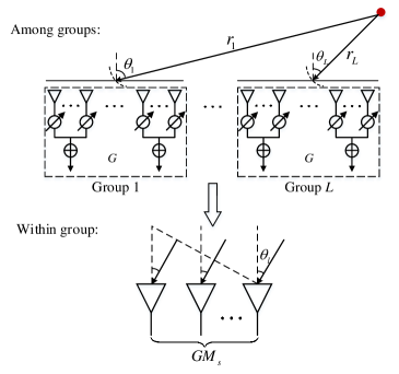
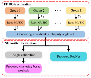
Figure 2: The proposed grouped HAD structure. (a) The different signal propagation models under the scenarios of inter groups and within each group. (b) The localization via grouped HAD structure has two steps, FF DOA estimation and NF localization.

III-A Model Transformation

An emitter can be viewed as NF if it falls in the Fresnel region of the receive array, which is defined as $r\in[0.62(D^{3}/\lambda)^{1/2},2D^{2}/\lambda]$. The range of Fresnel region depends both on $\lambda$ and $D$. By maintaining a constant distance between emitter and receive array, increasing the signal wavelength or reducing the array aperture can effectively decrease the extent of the Fresnel region, and leading to the conversion of signal model into planar wave-based FF model. Nevertheless, in practical scenarios, the signal wavelength and array aperture are typically predetermined, so making this conversion unattainable. In this paper, we partition the hybrid array into $L$ even groups, each group contains $G$ subarrays, i.e., $K=LG$, and thus each group also has $M_{g}=GM_{s}$ antennas. By treating each group as an independent array, the array aperture will be much smaller than the original receive array. Under the assumption that the following condition

$$r>\frac{2D_{g}^{2}}{\lambda}\Rightarrow D_{g}<\sqrt{\frac{r\lambda}{2}},$$ (7)

is met, where $D_{g}$ denotes the aperture of each group, it is feasible to regard the signal received within each group is planar wave and without changing the signal wavelength.

As depicted in Fig.2, for a comprehensive receive array, NF signal arrives in the form of spherical wave, so the signal directions detected at reference points of distinct groups are different. However, within each group, NF signal is converted into FF, resulting in all antennas within the same group detecting signals from the same direction. Consequently, a NF signal can be simplified as $L$ distinct FF signals received by $L$ respective arrays, and the signal model in (3) is transformed to

$$\mathbf{y}(t)=[\mathbf{y}_{1}^{T}(t)~{}\mathbf{y}_{2}^{T}(t)\cdots\mathbf{y}_{L}^{T}(t)]^{T},$$ (8)

where

$$\mathbf{y}_{l}(t)=\mathbf{W}_{l}^{H}\tilde{\mathbf{x}}_{l}=\mathbf{W}_{l}^{H}\left(\mathbf{a}(\theta_{l})s(t)+\mathbf{v}_{l}(t)\right)$$ (9)

is the received signal model of group $l$. $\mathbf{W}_{l}$ is a $M_{g}\times G$ block diagonal matrix as defined in (5), and

$$\mathbf{a}(\theta_{l}) =[1,e^{j\frac{2\pi}{\lambda}d\sin\theta_{l}},\cdots,e^{j\frac{2\pi}{\lambda}(GM_{s}-1)d\sin\theta_{l}}]^{T}$$ (10)

$$=\mathbf{a}_{g}(\theta_{l})\otimes\mathbf{a}_{s}(\theta_{l})\in\mathbb{C}^{GM_{s}\times 1}$$

is the array steering vector of group $l$, where $\theta_{l}$ is the DOA that detected by group $l$. $\mathbf{a}_{s}(\theta_{l})=[1,e^{j\frac{2\pi}{\lambda}d\sin\theta_{l}},\cdots,e^{j\frac{2\pi}{\lambda}(M_{s}-1)d\sin\theta_{l}}]^{T}\in\mathbb{C}^{M_{s}\times 1}$, and $\mathbf{a}_{g}(\theta_{l})=[1,e^{j\frac{2\pi}{\lambda}M_{s}d\sin\theta_{l}},\cdots,e^{j\frac{2\pi}{\lambda}(G-1)M_{s}d\sin\theta_{l}}]^{T}\in\mathbb{C}^{G\times 1}$ is generated by treating each subarray as an antenna and so group $l$ can be regarded as a $G$-elements array with inter-element spacing $M_{s}d$.

III-B Root-MUSIC for DOA Estimation via Grouped HAD Array

The covariance matrix of $\mathbf{y}_{l}(t)$ is given as

$$\mathbf{R}_{l}={\rm{E}}[\mathbf{y}_{l}(t)\mathbf{y}_{l}^{H}(t)]=\sigma_{s}^{2}\mathbf{a}_{W}(\theta_{l})\mathbf{a}_{W}^{H}(\theta_{l})+\sigma_{v}^{2}\mathbf{I}_{G}$$ (11)

where

$$\mathbf{a}_{W}(\theta_{l})=\mathbf{W}_{l}^{H}\mathbf{a}(\theta_{l})=\mathbf{W}_{l}^{H}\left(\mathbf{a}_{g}(\theta_{l})\otimes\mathbf{a}_{s}(\theta_{l})\right)\in\mathbb{C}^{G\times 1}.$$ (12)

Then the MUSIC spectrum can be obtained as

$$P(\theta_{l})=\frac{1}{\mathbf{a}^{H}_{W}(\theta_{l})\mathbf{U}_{N,l}\mathbf{U}_{N,l}^{H}\mathbf{a}_{W}(\theta_{l})},$$ (13)

where $\mathbf{U}_{N,l}\in\mathbb{C}^{G\times(G-1)}$ is corresponding to the noise subspace. By searching the peak of the pseudo-spectrum we can obtain the DOA estimation result of each group. The essence of MUSIC algorithm is based on grid search, which requires increasing the grid density to improve accuracy, but this will also lead to a rise in algorithm complexity. Therefore, Root-MUSIC algorithm is considered as a substitution, which has the characteristics of search-free and low-complexity [26].

Referring to the method in [24], we set the phases of phase shifters in the group $l$ to be identical, i.e., $\mathbf{w}_{1}=\cdots=\mathbf{w}_{G}=\frac{e^{j\alpha_{l}}}{\sqrt{M_{s}}}\bm{1}_{M_{s}}$, where $\bm{1}_{M_{s}}$ denotes an $M_{s}\times 1$ vector filled with element 1. Then we can get

$$\mathbf{W}_{l}=\mathbf{I}_{G}\otimes\mathbf{w}_{g},$$ (14)

and $\mathbf{a}_{W}(\theta_{l})$ can be further given as

$$\mathbf{a}_{W}(\theta_{l}) =(\mathbf{I}_{G}\otimes\mathbf{w}_{g}^{H})\left(\mathbf{a}_{g}(\theta_{l})\otimes\mathbf{a}_{s}(\theta_{l})\right)$$ (15)

$$=\mathbf{w}_{g}^{H}\mathbf{a}_{s}(\theta_{l})\mathbf{a}_{g}(\theta_{l}),$$

where

$$\mathbf{w}_{g}^{H}\mathbf{a}_{s}(\theta_{l}) =\frac{e^{j\alpha_{l}}}{\sqrt{M_{s}}}\sum_{m_{s}=1}^{M_{s}}e^{j\frac{2\pi}{\lambda}(m_{s}-1)d\sin\theta_{l}}$$ (16)

$$=\frac{e^{j\alpha_{l}}}{\sqrt{M_{s}}}\cdot\frac{1-e^{j\frac{2\pi}{\lambda}M_{s}d\sin\theta_{l}}}{1-e^{j\frac{2\pi}{\lambda}d\sin\theta_{l}}}.$$

So it makes sense that the new expression of $P(\theta_{l})$ is

$$P(\theta_{l})=\frac{1}{\lVert\mathbf{w}_{g}^{H}\mathbf{a}_{s}(\theta_{l})\rVert^{2}\mathbf{a}^{H}_{g}(\theta_{l})\mathbf{U}_{N}\mathbf{U}_{N}^{H}\mathbf{a}_{g}(\theta_{l})},$$ (17)

and let $\mathbf{C}=\mathbf{U}_{N}\mathbf{U}_{N}^{H}$, we can obtain

$$P^{-1}(\theta_{l})=\frac{2-e^{j\frac{2\pi}{\lambda}M_{s}d\sin\theta_{l}}-e^{-j\frac{2\pi}{\lambda}M_{s}d\sin\theta_{l}}}{2-e^{j\frac{2\pi}{\lambda}d\sin\theta_{l}}-e^{-j\frac{2\pi}{\lambda}d\sin\theta_{l}}}\cdot$$ (18)

$$\sum_{g_{1}=1}^{G}\sum_{g_{2}=1}^{G}e^{-j\frac{2\pi}{\lambda}(g_{1}-1)M_{s}d\sin\theta_{l}}\mathbf{C}_{g_{1},g_{2}}e^{j\frac{2\pi}{\lambda}(g_{2}-1)M_{s}d\sin\theta_{l}},$$

where $\mathbf{C}_{g_{1},g_{2}}$ denotes the element at the $g_{2}$th column of the $g_{1}$th row of $\mathbf{C}$. Then following the procedure of Root-MUSIC algorithm, we define $z_{l}=e^{j\frac{2\pi}{\lambda}M_{s}d\sin\theta_{l}}$ and the equivalent polynomial is

$$f(z_{l})=\frac{2-z_{l}-z_{l}^{-1}}{2-z_{l}^{\frac{1}{M_{s}}}-z_{l}^{-\frac{1}{M_{s}}}}\sum_{g_{1}=1}^{G}\sum_{g_{2}=1}^{G}z_{l}^{-(g_{1}-1)}\mathbf{C}_{g_{1},g_{2}}z_{l}^{g_{2}-1}.$$ (19)

Therefore, searching the peak of (13) is equivalent to evaluating the root of polynomial $f(z_{l})$ that be closest to the unit circle, which is denoted by $\hat{z}_{l}$, then the signal direction $\theta_{l}$ can be estimated as

$$\hat{\theta}_{l}=\arcsin\left(\frac{\lambda\arg\hat{z}_{l}}{2\pi M_{s}d}\right),$$ (20)

where $\arg$ is a function used to return the phase angle of a complex number. However, as each group is viewed as a $G$-elements ULA and its inter-elements spacing $M_{s}d=M_{s}\lambda/2$, this will cause an ambiguity with $M_{s}$ possible results in phase extraction. So in order to solve this ambiguity, we first rewritten (20) as

$$\hat{\theta}_{l}=\arcsin\left(\frac{\lambda(\arg\hat{z}_{l}+2\pi i)}{2\pi M_{s}d}\right),$$ (21)

where $i\in\{0,1,\cdots,M_{s}-1\}$ is the ambiguity coefficient. Then a solution set contained $M_{s}$ elements can be constructed for group $l$:

$$\hat{\Theta}_{l}=\left\{\hat{\theta}_{l,0},\hat{\theta}_{l,1},\cdots,\hat{\theta}_{l,M_{s}-1}\right\}\in\mathbb{R}^{M_{s}},$$ (22)

where $\hat{\Theta}_{l}$ is called initial set in this work, and $\hat{\theta}_{l,i}$ stands for the initial solution of group $l$ with ambiguity coefficient $i$. It is obviously that there is only one true solution in $\hat{\Theta}_{l}$, which is denoted by $\hat{\theta}_{l,true}=\theta_{l}$, and the rest solutions are false solutions. So the problem here is how to eliminate the false solutions, and thus obtaining the true position of NF emitter.

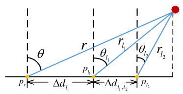
Figure 3: The geometric relationship between the reference points of various groups and the entire array in the NF model.

III-C Angle Calibration

Since the DOAs measured by $L$ groups are different from each other for the NF emitter, it is necessary to calibrate them to a common point to obtain the final DOA estimation result. As shown in Fig.3, $p_{r}$ is a reference point of the whole receive array, $p_{l_{1}}$ and $p_{l_{2}}$ denote the reference points of group $l_{1}$ and $l_{2}$, where $1\leq l_{1}<l_{2}\leq L$. Then the position of the emitter relative to these three reference points can be respectively represented as $(\theta,r)$, $(\theta_{l_{1}},r_{l_{1}})$ and $(\theta_{l_{2}},r_{l_{2}})$, where $\theta_{l_{1}}$ and $\theta_{l_{2}}$ are the initial solutions of group $l_{1}$ and $l_{2}$ that can be obtained by (21). From the Fig.3, we can see $(\theta,r)$ can be expressed by $(\theta_{l_{1}},r_{l_{1}})$ and $(\theta_{l_{2}},r_{l_{2}})$ based on their geometrical relationship, and because there are four unknown parameters: $\theta$, $r$, $r_{l_{1}}$ and $r_{l_{2}}$, at least four independent equations are needed to solve this problem. So the following equations are established:

$$r_{l_{1}}\cos\theta_{l_{1}}=r_{l_{2}}\cos\theta_{l_{2}}$$ (23a)

$$r_{l_{1}}\sin\theta_{l_{1}}=r_{l_{2}}\sin\theta_{l_{2}}+\Delta d_{l_{1},l_{2}}$$ (23b)

$$r\cos\theta=r_{l_{2}}\cos\theta_{l_{2}}$$ (23c)

$$r\sin\theta=r_{l_{2}}\sin\theta_{l_{2}}+\Delta d_{l_{2}}$$ (23d)

where $\Delta d_{l_{1},l_{2}}=(l_{2}-l_{1})GM_{s}d$ denotes the distance between $p_{l_{1}}$ and $p_{l_{2}}$, $\Delta d_{l_{2}}=\Delta d_{l_{1}}+\Delta d_{l_{1},l_{2}}$ is the distance between $p_{r}$ and $p_{l_{2}}$. Firstly, substituting (23a) into (23b), we can get the expression of $r_{l_{2}}$

$$r_{l_{2}}=\frac{\Delta d_{l_{1},l_{2}}\cos\theta_{l_{1}}}{\sin\theta_{l_{1}}\cos\theta_{l_{2}}-\cos\theta_{l_{1}}\sin\theta_{l_{2}}},$$ (24)

then from (23c) we can know $r=r_{l_{2}}\cos\theta_{l_{2}}/\cos\theta$, and substituting (24) into (23d), the following equation is generated

$$\tan\theta=\frac{\Delta d_{l_{2}}\tan\theta_{l_{1}}-\Delta d_{l_{1}}\tan\theta_{l_{2}}}{\Delta d_{l_{1},l_{2}}}.$$ (25)

By substituting the DOAs estimated by any two groups, the calibrated $\theta$ can also be obtained as

$$\hat{\theta}_{l_{1},l_{2}}=\arctan\left(\frac{\Delta d_{l_{2}}\tan\hat{\theta}_{l_{1}}-\Delta d_{l_{1}}\tan\hat{\theta}_{l_{2}}}{\Delta d_{l_{1},l_{2}}}\right),$$ (26)

where $\hat{\theta}_{l_{1},l_{2}}$ represents the calibrated angle solution obtained by combining group ${l_{1}}$ and group ${l_{2}}$. As the reference point of a receive array is usually located at the first antenna, then $p_{r}$ and $p_{l_{1}}$ are overlapped when $l_{1}=1$, and from Fig.3 we know $\Delta d_{1}=0$ and $\Delta d_{1,l_{2}}=\Delta d_{l_{2}}$ in this case. Therefore, based on (26) we can get

$$\hat{\theta}_{1,l_{2}}=\arctan(\hat{\theta}_{1})=\begin{cases}\hat{\theta}_{1},&-\frac{\pi}{2}\leq\hat{\theta}_{1}\leq\frac{\pi}{2}\\ \hat{\theta}_{1}-\pi,&\hat{\theta}_{1}>\frac{\pi}{2}\\ \hat{\theta}_{1}+\pi,&\hat{\theta}_{1}<-\frac{\pi}{2}\end{cases},$$ (27)

where $2\leq l_{2}\leq L$. Because the range of $\theta$ is restricted in $[-\pi/2,\pi/2]$, if $\hat{\theta}_{1,l_{2}}\neq\hat{\theta}_{1}$, the corresponding $\hat{\theta}_{1}$ is a definite false solution.

Since the ambiguity coefficient has not been determined, the calibrated set also contains one true solution and $M_{s}-1$ false solutions, just like (22):

$$\hat{\Theta}_{l_{1},l_{2}}=\left\{\hat{\theta}_{l_{1},l_{2},0},\hat{\theta}_{l_{1},l_{2},1},\cdots,\hat{\theta}_{l_{1},l_{2},M_{s}-1}\right\}\in\mathbb{R}^{M_{s}},$$ (28)

and the true solution of this set is denoted by $\hat{\theta}_{l_{1},l_{2},i_{t}}$. Theoretically, the true solutions of different sets are identical, i.e.,

$$\hat{\theta}_{1,2,i_{t}}=\cdots=\hat{\theta}_{L-1,L,i_{t}}=\theta,$$ (29)

where $i_{t}$ denotes the true ambiguity coefficient. And the false solutions are usually different from each other. Then combining all $L$ groups, we can get a calibrated angle set

$$\hat{\Theta}=\hat{\Theta}_{1,2}\cup\hat{\Theta}_{1,3}\cup\cdots\cup\hat{\Theta}_{L-1,L}\in\mathbb{R}^{NM_{s}},$$ (30)

where $N={L\choose 2}$.

As the range parameter $r$ can be obtained by (23c), then the calibrated range set is also given as

$$\hat{\mathcal{R}}=\hat{\mathcal{R}}_{1,2}\cup\hat{\mathcal{R}}_{1,3}\cup\cdots\cup\hat{\mathcal{R}}_{L-1,L}\in\mathbb{R}^{NM_{s}},$$ (31)

where $\hat{\mathcal{R}}_{l_{1},l_{2}}=\left\{\hat{r}_{l_{1},l_{2},0},\hat{r}_{l_{1},l_{2},1},\cdots,\hat{r}_{l_{1},l_{2},M_{s}-1}\right\}$ and

$$\hat{r}_{l_{1},l_{2},i}=\frac{\hat{r}_{l_{2},i}\cos\hat{\theta}_{l_{2},i}}{\cos\hat{\theta}_{l_{1},l_{2},i}}.$$ (32)

The true solutions of subsets that compose $\hat{\mathcal{R}}$ also satisfy

$$\hat{r}_{1,2,i_{t}}=\cdots=\hat{r}_{L-1,L,i_{t}}=r.$$ (33)

By matching the elements in $\hat{\Theta}$ and $\hat{\mathcal{R}}$ one by one, we can get a calibrated position set for the NF emitter

$$\Omega=\left\{\bm{\omega}_{l_{1},l_{2},i}\big{|}1\leq l_{1}<l_{2}\leq L,~{}0\leq i\leq M_{s}-1\right\},$$ (34)

where $\omega_{l_{1},l_{2},i}=(\hat{\theta}_{l_{1},l_{2},i},\hat{r}_{l_{1},l_{2},i})$ and $|\Omega|=NM_{s}$. In the next section, we will discuss how to eliminate the false solutions of $\Omega$ and obtain the true position of the NF emitter.

IV Proposed Low-Complexity Clustering-based Methods for NF Localization

In this section, to infer the true angles and achieve the localization of NF emitter, two clustering-methods are designed based on the data distribution features of the candidate position set.

IV-A Minimum sample distance clustering

As the position of NF emitter can not be calculated before the ambiguity coefficient is determined, we have to find out the special characters of the true solutions to discriminate them from the false solutions in $\Omega$. Based on different ambiguity coefficients, $\Omega$ can be naturally divided into $M_{s}$ subsets:

$$\Omega=\Omega_{0}\cup\Omega_{1}\cup\cdots\cup\Omega_{M_{s}-1},$$ (35)

where

$$\Omega_{i}=\left\{\bm{\omega}_{l_{1},l_{2},i}\big{|}1\leq l_{1}<l_{2}\leq L\right\},$$ (36)

and $|\Omega_{i}|=N$. Among theses $M_{s}$ subsets, there are one true set and $M_{s}-1$ false sets. The true set is given as

$$\Omega_{true}=\left\{\bm{\omega}_{l_{1},l_{2},i_{t}}\big{|}1\leq l_{1}<l_{2}\leq L\right\},$$ (37)

where $\bm{\omega}_{l_{1},l_{2},i_{t}}=(\hat{\theta}_{l_{1},l_{2},i_{t}},\hat{r}_{l_{1},l_{2},i_{t}})$. Based on (29) and (33), we have $\bm{\omega}_{1,2,i_{t}}=\cdots=\bm{\omega}_{L-1,L,i_{t}}$.

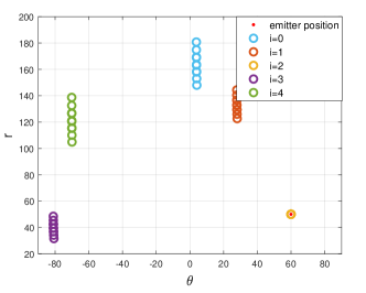
Figure 4: The calibrated candidate emitter positions discriminated by ambiguity coefficient in the $(\theta,r)$-plane.

In Fig.4, we plot the points of (34) in a coordinate with angle as $x$-axis and distance as $y$-axis in the noise-free situation, the actual position of the emitter relative to the receive array is $(60^{\circ},50m)$. A cluster in this diagram is corresponding to an $\Omega_{i}$, the true ambiguity coefficient is $i_{true}=2$ in this case, and thus the samples of cluster 2 are gathered together, while the samples of other clusters are scattered especially in the distance dimension.

Based on the distribution characters of the calibrated points in the $(\theta,r)$-diagram, the true solution set $\Omega_{true}$ can be distinguished via finding the most concentration one among all the $M_{s}$ clusters. Here the scatter degree of a cluster is defined by the summation of the distance between any two samples in this cluster, and the squared Euclidean distance (SED) is employed as distance measure. Then we can get the distance between two samples as

$$d_{n_{1},n_{2}}^{i}=\lVert\bm{\omega}_{n_{1},i}-\bm{\omega}_{n_{2},i}\rVert^{2}$$ (38)

where $1\leq n_{1}<n_{2}\leq N$. Here $\bm{\omega}_{l_{1},l_{2},i}$ is simplified to $\bm{\omega}_{n,i}$ for convenient expression. And the scatter degree of cluster $i$ is defined as

$$\bar{d}_{i}=\sum_{n_{1}=1}^{N-1}\sum_{n_{2}=n_{1}+1}^{N}d_{n_{1},n_{2}}^{i}.$$ (39)

It’s obviously that the smaller value of $\bar{d}_{i}$ represents the corresponding cluster has high concentration, so the optimization problem is given as

$$\hat{i}=\arg\min_{i}\bar{d}_{i},$$ (40)

Then the final estimation results of $\theta$ and $r$ can also be given as

$$\hat{\theta}=\frac{1}{N}\sum_{n=1}^{N}\hat{\theta}_{n,\hat{i}},\quad\hat{r}=\frac{1}{N}\sum_{n=1}^{N}\hat{r}_{n,\hat{i}},$$ (41)

and the estimated NF emitter position is $(\hat{\theta},\hat{r})$.

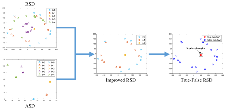
Figure 5: The proposed clustering method for NF emitter localization by combining RSD and ASD.

IV-B RSD-ASD-based Density clustering

In Fig.4, the candidate emitter positions are plotted in the $(\theta,r)$ diagram, and the distribution characteristics of the calibrated points are extracted by combining the angle and range dimensions. But we can also find that these points have different distributions in angle and range dimensions. Therefore, in order to further explore the distribution characteristics of different dimensions and improve the emitter localization accuracy, we decide to construct the angle scatter diagram (ASD) and range scatter diagram (RSD) respectively as shown in Fig.5. As the elements of $\hat{\Theta}$ and $\hat{\mathcal{R}}$ just have one dimension, so we need to make a transformation that allow them to be scattered in a 2D plane. Then we first get the polarization forms of $\theta$ and $r$:

$$\tilde{\theta}=\theta e^{j\theta},~{}~{}\tilde{r}=re^{jr},$$ (42)

and by extracting their real and image parts respectively, the real numbers are transformed to two-dimensional vectors, i.e., $(\Re(\tilde{\theta}),\Im(\tilde{\theta}))$ and $(\Re(\tilde{r}),\Im(\tilde{r}))$. In the following content, we will introduce how to construct RSD and ASD based on this transformation, and thus achieving high-accuracy localization of NF emitter.

Firstly, we perform the transformation on the calibrated range set $\hat{\mathcal{R}}$ and get

$$\tilde{\mathcal{R}}=\left\{\tilde{\bm{\omega}}^{r}_{l_{1},l_{2},i}\big{|}1\leq l_{1}<l_{2}\leq L,0\leq i\leq M_{s}-1\right\},$$ (43)

where $|\tilde{\mathcal{R}}|=NM_{s}$, $\tilde{\bm{\omega}}^{r}_{l_{1},l_{2},i}=(\Re(\tilde{r}_{l_{1},l_{2},i}),\Im(\tilde{r}_{l_{1},l_{2},i}))$ and $\tilde{r}_{l_{1},l_{2},i}=\hat{r}_{l_{1},l_{2},i}e^{j\hat{r}_{l_{1},l_{2},i}}$. $\tilde{\mathcal{R}}$ can also be divided into $M_{s}$ subsets based on different ambiguity coefficients as $\tilde{\mathcal{R}}=\tilde{\mathcal{R}}_{0}\cup\tilde{\mathcal{R}}_{1}\cup\cdots\cup\tilde{\mathcal{R}}_{M_{s}-1}$, and the true solution set therein is given as

$$\tilde{\mathcal{R}}_{true}=\left\{\tilde{\bm{\omega}}^{r}_{l_{1},l_{2},i_{t}}\big{|}1\leq l_{1}<l_{2}\leq L\right\},$$ (44)

where $\tilde{\bm{\omega}}^{r}_{1,2,i_{t}}=\cdots=\tilde{\bm{\omega}}^{r}_{L-1,L,i_{t}}$. Compared to Fig.4, the false solutions in the proposed RSD are more scattered, and the true solutions are still inseparable, so RSD is more suitable for the application of high-performance clustering methods.

In order to weaken the impact of false solutions on the final localization result, based on (27) and the related conclusions, we construct a new candidate angle set as

$$\mathcal{A}=\hat{\Theta}_{1}\cup\hat{\Theta}_{1,2}\cup\hat{\Theta}_{1,3}\cup\cdots\cup\hat{\Theta}_{1,L}\in\mathbb{R}^{LM_{s}},$$ (45)

where $\hat{\Theta}_{1}$ is defined in (22), and $\hat{\Theta}_{1,2}$ to $\hat{\Theta}_{1,L}$ are defined in (28). Then the polarization forms of the elements in $\mathcal{A}$ can be obtained and the set is transformed to

$$\tilde{\mathcal{A}}= \left\{\tilde{\bm{\omega}}^{\theta}_{1,i}\big{|}0\leq i\leq M_{s}-1\right\}\cup$$ (46)

$$\left\{\tilde{\bm{\omega}}^{\theta}_{1,l,i}\big{|}2\leq l\leq L,0\leq i\leq M_{s}-1\right\},$$

where $|\tilde{\mathcal{A}}|=LM_{s}$, $\tilde{\bm{\omega}}^{\theta}_{1,i}=(\Re(\tilde{\theta}_{1,i}),\Im(\tilde{\theta}_{1,i}))$ and $\tilde{\theta}_{1,i}=\hat{\theta}_{1,i}e^{j\hat{\theta}_{1,i}}$, $\tilde{\omega}^{\theta}_{1,l,i}=(\Re(\tilde{\theta}_{1,l,i}),\Im(\tilde{\theta}_{1,l,i}))$ and $\tilde{\theta}_{1,l,i}=\hat{\theta}_{1,l,i}e^{j\hat{\theta}_{1,l,i}}$. So the ASD in Fig.5 is constructed by the points of $\tilde{\mathcal{A}}$, and to be distinguished easily, $\tilde{\bm{\omega}}^{\theta}_{1,i}$ is plotted by triangular symbol. From (27), we can know if $i$ is the true ambiguity coefficient, then $\tilde{\bm{\omega}}^{\theta}_{1,i}=\tilde{\bm{\omega}}^{\theta}_{1,2,i}=\cdots=\tilde{\bm{\omega}}^{\theta}_{1,L,i}$ is the necessary and insufficient condition. But it’s obviously that the clusters of $i=3$ and $i=4$ in the ASD can’t satisfy this condition, so they can be labeled as false ambiguity coefficients directly and the corresponding angles are false solutions.

By combining RSD and ASD, we can eliminate a part of false solutions of $\tilde{\mathcal{R}}$ corresponding to $i$ which have been labeled as false ambiguity coefficients by ASD, then the improved range solution set is obtained as

$$\tilde{\mathcal{R}}_{imp}=\tilde{\mathcal{R}}_{imp,1}\cup\cdots\cup\tilde{\mathcal{R}}_{imp,M_{imp}},$$ (47)

where $M_{imp}\leq M_{s}$ denotes the number of remaining subsets after the false solution sets elimination and $|\tilde{\mathcal{R}}_{imp}|=NM_{imp}$, thereby generating the improved RSD. The step 3 of algorithm 1 describes how to eliminate the false solutions based on $\tilde{\mathcal{A}}$ in the actual operations, where $\varepsilon$ is a threshold which decreases with the increasing of $\rm{SNR}$ and $\varepsilon=0$ under the noise-free condition. Compared to the initial RSD, the improved RSD has less false solutions, and thus the true solutions are easier to be identified. Then since the true solutions gather together, density-based clustering methods can be considered for inferring the true solutions.

As the most representative algorithm for density-based clustering, the core idea of DBSCAN [27] is to measure the space density of a sample point by the number of points within its neighborhood. Therefore, there are two parameters requiring to be given before clustering: $\epsilon$, the radius of neighborhood, and $MinPts$ denotes the minimum number of sample points that contained in the $\epsilon$-neighborhood. Next we will introduce how to determine the neighborhood parameter based on our problem. Since the true solution set $\tilde{\mathcal{R}}_{true}$ has $N$ points, we can get $MinPts=N$. Then in order to obtain the neighborhood range $\epsilon$, first we calculate the distances between all sample points within each subset of $\tilde{\mathcal{R}}_{imp}$, and then find the maximum value among them

$$d_{m,max}=\max\left\{\lVert\bm{\omega}_{m,n_{1}}^{r}-\bm{\omega}_{m,n_{2}}^{r}\rVert^{2}|1\leq n_{1}<n_{2}\leq N\right\},$$ (48)

where $\bm{\omega}_{m,n}^{r}$ denotes the $n$-th elements of $\tilde{\mathcal{R}}_{imp,m}$ and $1\leq m\leq M_{imp}$. Due to the elements of true solution set have the tightest connections, so the value of $\epsilon$ is set as the minimum $d_{m,max}$, i.e.,

$$\epsilon=\min\left\{d_{m,max}|1\leq m\leq M_{imp}\right\}.$$ (49)

Since the required parameters are determined, we can perform clustering on sample set $\tilde{\mathcal{R}}_{imp}$ via DBSCAN, and the clustering procedure can be summarized as: (1) find out the samples that have at least $N$ points in their $\epsilon$-neighborhoods and label their as core objects, (2) all the core objects that are density-connected and the points in their neighborhoods are divided into the same clusters. Then the clustering result can be expressed by

$$\left\{\mathcal{C}_{n_{c}}|1\leq n_{c}\leq N_{c}\right\}={\rm{DBSCAN}}\left(\tilde{\mathcal{R}}_{imp},(\epsilon,N)\right)$$ (50)

where $N_{c}$ denotes the number of clusters. Next, we seek out the cluster $\mathcal{C}_{n_{c}}=\mathcal{C}_{max}$ that has the most points, i.e., $|\mathcal{C}_{max}|=\max\{|\mathcal{C}_{1}|,|\mathcal{C}_{2}|,\cdots,|\mathcal{C}_{N_{c}}|\}$. Since the task is to find the $N$ true solutions, if $|\mathcal{C}_{max}|=N$ we can get $\tilde{\mathcal{R}}_{true}=\mathcal{C}_{max}$, but if $|\mathcal{C}_{max}|>N$, it needs to be further divided until $|\mathcal{C}_{max}|=N$ is achieved. In this process, the neighborhood radius $\epsilon$ should be reduced in each iteration, and the renewed $\epsilon$ is given as

$$\epsilon_{j}=\eta_{j}\epsilon_{j-1},$$ (51)

where $j$ denotes the iteration number and $\eta_{j}<1$ is an adjustable coefficient.

Algorithm 1 RSD-ASD-DBSCAN

$\hat{\Theta}_{1}$, $\hat{\Theta}$, $\hat{\mathcal{R}}$;

1: transform $\hat{\mathcal{R}}$ to point set $\tilde{\mathcal{R}}$, where $|\tilde{\mathcal{R}}|=NM_{s}$, and generate RSD;

2: obtain $\tilde{\mathcal{A}}$ by combining $\hat{\Theta}_{1}$ and $\hat{\Theta}$, where $|\tilde{\mathcal{A}}|=LM_{s}$, and generate ASD;

3: given $\tilde{\mathcal{R}}_{imp}=\tilde{\mathcal{R}}$, eliminate some false solutions by performing the following steps:

  3.1: for $i=0,1,\cdots,M_{s}-1$ do

  3.2:    if $\sum_{l=2}^{L}\lVert\tilde{\omega}^{\theta}_{1,l,i}-\tilde{\omega}^{\theta}_{1,i}\rVert^{2}>\varepsilon$

  3.3:     $\tilde{\mathcal{R}}_{imp}=\tilde{\mathcal{R}}_{imp}/\tilde{\mathcal{R}}_{i}$;

  3.4:    else

  3.5:     $\tilde{\mathcal{R}}_{imp}=\tilde{\mathcal{R}}_{imp}$;

  3.6:    end if

  3.7: end for

4: given the initial neighborhood parameters $(\epsilon_{0},N)$ and implement DBSCAN on $\tilde{\mathcal{R}}_{imp}$, find out the cluster $\mathcal{C}_{max,0}$ that has the highest density, then obtain the true distance solution set by following judgment:

  4.1: while $|\mathcal{C}_{max,j-1}|>N$ do

  4.2:  $\epsilon_{j}=\eta_{j}\epsilon_{j-1}$;

  4.3:  implement (50) and find out $\mathcal{C}_{max,j}$;

  4.4:  $\tilde{\mathcal{R}}_{imp}=\mathcal{C}_{max,j}$;

  4.5:  $j=j+1$;

  4.6: end while

5: obtain the true angle solution set from (34);

6: calculate the range and angle estimation results based on (52) and (53);

$\hat{r}$, $\hat{\theta}$.

With the obtained true point set $\tilde{\mathcal{R}}_{true}=\{\tilde{\omega}_{true,1},\tilde{\omega}_{true,2}\cdots\tilde{\omega}_{true,N}\}$, where $\tilde{\omega}_{true,n}=(\Re(\tilde{r}_{true,n}),\Im(\tilde{r}_{true,n}))$, we can get the true range solution set $\hat{\mathcal{R}}_{true}=\{\hat{r}_{true,1},\hat{r}_{true,2},\cdots,\hat{r}_{true,N}\}$ recovered from $\tilde{\mathcal{R}}_{true}$ based on (42), where $\hat{r}_{true,n}=|\tilde{\omega}_{true,n}|$. Then the range estimation result is given as

$$\hat{r}=\frac{1}{N}\sum_{n=1}^{N}\hat{r}_{true,n}.$$ (52)

Since the initial sample set $\tilde{\mathcal{R}}_{imp}$ comes from the calibrated distance set (31) and $\tilde{\mathcal{R}}_{true}\subseteq\tilde{\mathcal{R}}_{imp}$, then we can get $\hat{\mathcal{R}}_{true}\subset\hat{\mathcal{R}}$. So we can always find a corresponding angle $\hat{\theta}_{true,n}$ for $\hat{r}_{true,n}$ from $\Omega$, and the angle estimation result can also be given as

$$\hat{\theta}=\frac{1}{N}\sum_{n=1}^{N}\hat{\theta}_{true,n}.$$ (53)

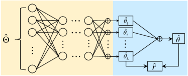
Figure 6: The proposed RegNet for NF localization, where the yellow part is a MLNN that performs false solutions elimination and the blue part is a perceptron for angle fusion.

V Proposed Regression Network for High-resolution NF Localization

In this section, a regression network is proposed for achieving higher localization accuracy by combining the functions of false solution elimination and true solution fusion.

V-A Network Construction

By combining the solution sets of all the groups, we can get

$$\hat{\Theta}=\hat{\Theta}_{1}\cup\hat{\Theta}_{2}\cup\cdots\cup\hat{\Theta}_{L}\in\mathbb{R}^{LM_{s}},$$ (54)

from the generation mechanism of the phase ambiguity we can know there are $L(M_{s}-1)$ false solutions in $\hat{\Theta}$, so the task of phase ambiguity elimination is to find out the $L$ true solution from all $LM_{s}$ solutions. As this process is nonlinear, then it can be simply expressed as

$$\hat{\Theta}_{true}=f_{nl}(\hat{\Theta}),$$ (55)

where $\hat{\Theta}_{true}=\{\hat{\theta}_{1,true},\cdots,\hat{\theta}_{L,true}\}$ and $f_{nl}(\cdot)$ denotes an $LM_{s}$-dimension to $L$-dimension nonlinear mapping. By observing (55) we can find, since we only know the input and output, and don’t know the concrete mapping relationship, thus this problem can’t be transformed and solved by linear optimization algorithms. Then machine learning-based methods are usually adopted to solve problems like this. Depending on the specific situations and goals to be achieved, common methods include kernel methods [28], neural networks [29][30], non-parametric methods [31], etc. Among them, neural networks have the best performance for they can learn complex nonlinear mapping relationships through multiple layers of nonlinear transformations. Therefore, we will design a multi-layer neural network (MLNN) for solving the problem (55).

As shown in the yellow part of Fig.6, the input data is $\hat{\Theta}$, so the input layer of this MLNN contains $LM_{s}$ neurons, and the output layer has $L$ neurons for the output is $\hat{\Theta}_{true}$. Supposing the MLNN has $H$ hidden layers, then (55) is transformed to

$$\hat{\bm{\Theta}}_{true}=f^{(\rm{out})}(f^{(H)}(\cdots f^{(1)}(\mathbf{W}^{(\rm{in})}\hat{\bm{\Theta}}+\mathbf{b}^{(\rm{in})}))),$$ (56)

where $\hat{\bm{\Theta}}_{true}=[\hat{\theta}_{1,true},\cdots,\hat{\theta}_{L,true}]^{T}\in\mathbb{R}^{L\times 1}$ and $\hat{\bm{\Theta}}=[\hat{\theta}_{1,0},\cdots,\hat{\theta}_{1,M_{s}-1},\cdots,\hat{\theta}_{L,0},\cdots,\hat{\theta}_{L,M_{s}-1}]^{T}\in\mathbb{R}^{LM_{s}\times 1}$ are vectors that including the elements of sets $\hat{\Theta}_{true}$ and $\hat{{\Theta}}$, $\mathbf{W}^{(\rm{in})}$ and $\mathbf{b}^{(\rm{in})}$ are weight and bias vectors of input layer, $f^{(h)}(\cdot)$ represents the nonlinear transformation of the $h$th hidden layer. As the nonlinear modeling ability of neural networks comes from the activation functions, so here rectification linear unit (ReLU) is adopted as activation functions for the hidden layers. Finally, the expected output vector $\hat{\bm{\Theta}}_{true}$ contains $L$ specific angles, so this MLNN is designed for achieving a regression task, then the output layer can adopt linear activation function.

Since the emitter is an NF emitter, the true solutions of $L$ groups are different from each other, i.e., $\hat{\theta}_{1,true}\neq\hat{\theta}_{2,true}\neq\cdots\neq\hat{\theta}_{L,true}$. Therefore, $\hat{\bm{\Theta}}_{true}$ isn’t the final DOA estimation result, we have to design another method to fuse these true solutions. As there must be a linear transformation between two numbers, the fusion function can be given as the linear combination of the $L$ angles:

$$\hat{\theta}_{true}=\sum_{l=1}^{L}\beta_{l}f_{l}(\hat{\theta}_{l,true}),$$ (57)

where $\beta_{l}$ is the combination coefficient and $f_{l}(\cdot)$ denotes a linear transformation. Due to the optimal $\beta_{l}$ and transformation relationship are unknown, we can design a perceptron like the blue part of Fig.6 to solve this problem, and thus (57) is transformed to

$$\hat{\theta}_{true} =f^{(p)}(\hat{\bm{\Theta}}_{true})$$ (58)

$$=\mathbf{W}^{(p)}\hat{\bm{\Theta}}_{true}+\mathbf{b}^{(p)},$$

where $\mathbf{W}^{(p)}$ and $\mathbf{b}^{(p)}$ are weight and bias vectors of this peceptron. So the proposed RegNet is the combination of the MLNN and perceptron, and the whole DOA estimation process can be expressed by

$$\hat{\theta}=\mathbf{W}^{(p)}f^{(\rm{out})}(f^{(H)}(\cdots f^{(1)}(\mathbf{W}^{(\rm{in})}\hat{\bm{\Theta}}+\mathbf{b}^{(\rm{in})})))+\mathbf{b}^{(p)}.$$ (59)

As the angle has been estimated, the next step is to estimate the range between emitter and receive array. Based on equations (23c) and (24), with the angle estimation result and the true angle solutions of all the groups, the range parameter can be obtained by

$$\hat{r}_{l_{1},l_{2}}=\frac{\Delta d_{l_{1},l_{2}}\cos\hat{\theta}_{l_{1}}\cos\hat{\theta}_{l_{2}}}{\cos\hat{\theta}(\sin\hat{\theta}_{l_{1}}\cos\hat{\theta}_{l_{2}}-\cos\hat{\theta}_{l_{1}}\sin\hat{\theta}_{l_{2}})}.$$ (60)

Since $L$ groups can conduct $N={L\choose 2}$ combinations, then the final result is the average of these $N$ estimations

$$\hat{r}=\frac{1}{N}\sum_{l_{1}=1}^{L-1}\sum_{l_{2}=l_{1}+1}^{L}\hat{r}_{l_{1},l_{2}}.$$ (61)

V-B Training Strategy

The input of the MLNN is $\hat{\bm{\Theta}}$, and the expected output is $\hat{\bm{\Theta}}_{true}$, so the training data and label pair is given as $(\hat{\bm{\Theta}},\hat{\bm{\Theta}}_{true})$. And as the range of DOA is $[-\pi/2,\pi/2]$, different angles can generate different training data and label pairs, then the complete training set can be expressed by $\{(\hat{\bm{\Theta}}^{\theta},\hat{\bm{\Theta}}^{\theta}_{true})|\theta\in[-\pi/2,\pi/2]\}$. In the training stage, we choose mean square error (MSE) as the loss function, which is defined as

$${\rm{MSE}}=\frac{1}{LN_{d}}\sum_{t=1}^{N_{d}}\sum_{l=1}^{L}\left(\hat{\theta}_{t,l,true}-\theta_{l,true}\right)^{2},$$ (62)

where $N_{d}$ denotes the number of training data and the $\theta_{l,true}$ is the ideal output of the $l$th output neuron. Then by minimizing (63) the optimal parameters of the proposed MLNN can be obtained. Similarly, the training set of the perceptron is $\{(\hat{\bm{\Theta}}^{\theta}_{true},\theta)|\theta\in[-\pi/2,\pi/2]\}$, and the loss function is also MSE:

$${\rm{MSE}}_{p}=\frac{1}{N_{d}}\sum_{t=1}^{N_{d}}\left(\hat{\theta}_{t,true}-\theta\right)^{2}.$$ (63)

Obviously, if we only want to obtain the angle information, theses two parts can be combined as an ensemble for reducing training complexity.

VI Performance Analysis

VI-A Complexity Analysis

From Fig.2 we can know the proposed methods share the common computation complexity from the Root-MUSIC algorithm in the FF DOA estimation stage, and have different computation complexities for the NF emitter localization. The computation complexity of Root-MUSIC comes from covariance matrix computation, SVD and signal subspace extraction, it can be approximately given as $\mathcal{O}(L(TG^{2}+G^{3}))$, where $G=M/(LM_{s})$. As a key step of clustering-based methods, the complexity of angle calibration is $\mathcal{O}(2NMs)$. Then the computation complexity of the proposed MSDC in the NF emitter localization stage only comes from computing the sample distance, so it is $\mathcal{O}(M_{s}N(N-1)/2)$. For the proposed RSD-ASD-DBSCAN, its complexity depends on the number of samples and how many iterations are required to find the only cluster that has $N$ samples, so it is given as $\mathcal{O}(\sum_{j=1}^{J}N_{s,j}^{2})$, where $N_{s,j}>N$ denotes the number of samples to be divided at $j$th iteration. Finally, the complexity of the proposed RegNet is related to the size of the MLNN, i.e., the depth and the number of neurons contained in each hidden layer. Then it is approximately given as $\mathcal{O}(N_{e}L^{2}M_{s}\prod_{h=1}^{H}N_{h})$, where $N_{e}$ denotes the number of epochs and $N_{h}$ is the neuron number of hidden layers.

TABLE I: Computation Complexity of Proposed Methods

Methods	Complexity
Proposed MSDC	$\mathcal{O}(TM^{2}/(LM_{s}^{2})+M^{3}/(LM_{s}^{3})+2NMs+M_{s}N(N-1)/2)$
Proposed RSD-ASD-DBSCAN	$\mathcal{O}(TM^{2}/(LM_{s}^{2})+M^{3}/(LM_{s}^{3})+\sum_{j=1}^{J}N_{s,j}^{2})$
Proposed RegNet	$\mathcal{O}(TM^{2}/(LM_{s}^{2})+M^{3}/(LM_{s}^{3})+N_{e}L^{2}M_{s}\prod_{h=1}^{H}N_{h})$

VI-B CRLB Analysis

The CRLB provides a lower bound on the variance of any unbiased estimator. So the CRLB of the grouped hybrid architecture is derived in this section as a benchmark to evaluate the NF localization performance of the proposed methods. Since the signal model (8) is only related to angle parameter, we have to first transform it to NF model. Based on the geometric relationship depicted in Fig.3 we get

$$\begin{cases}r_{l}\cos\theta_{l}=r\cos\theta_{l}\\ r_{l}\sin\theta_{l}=r\sin\theta-\Delta d_{l}\end{cases},$$ (64)

where $l=1,2,\cdots,L$ and $\Delta d_{l}=(l-1)GM_{s}d$. So we can express $\sin\theta_{l}$ by

$$\varphi_{l}=\sin\theta_{l}=\frac{r\sin\theta-\Delta d_{l}}{\sqrt{r^{2}-2\Delta d_{l}r\sin\theta+\Delta d_{l}^{2}}},$$ (65)

and the steering vector (10) also becomes

$$\mathbf{a}(\varphi_{l}) =\mathbf{a}_{g}(\varphi_{l})\otimes\mathbf{a}_{s}(\varphi_{l})$$ (66)

$$=[1,e^{j\frac{2\pi d}{\lambda}\varphi_{l}},\cdots,e^{j\frac{2\pi d}{\lambda}(GM_{s}-1)\varphi_{l}}]^{T},$$

where $\mathbf{a}_{s}(\varphi_{l})=[1,e^{j\frac{2\pi d}{\lambda}\varphi_{l}},\cdots,e^{j\frac{2\pi d}{\lambda}(M_{s}-1)\varphi_{l}}]^{T}$, and $\mathbf{a}_{g}(\theta_{l})=[1,e^{j\frac{2\pi d}{\lambda}M_{s}\varphi_{l}},\cdots,e^{j\frac{2\pi d}{\lambda}(G-1)M_{s}\varphi_{l}}]^{T}$. So the covariance matrix of group $l$ is given as

$$\mathbf{R}_{l}=\sigma_{s}^{2}\mathbf{a}_{W}(\varphi_{l})\mathbf{a}_{W}^{H}(\varphi_{l})+\sigma_{v}^{2}\mathbf{I}_{G},$$ (67)

where $\mathbf{a}_{W}(\varphi_{l})=\mathbf{W}_{l}^{H}\mathbf{a}(\varphi_{l})$. Then by combining all the groups we can get

$$\mathbf{R}={\rm{diag}}\{\mathbf{R}_{1},\mathbf{R}_{2},\cdots,\mathbf{R}_{L}\},$$ (68)

and the CRLB can be derived based on it.

Lemma 1: The CRLBs for the DOA and range estimations of grouped hybrid architecture can be expressed by

$${\rm{CRLB}}_{\theta}=\frac{\sum_{l=1}^{L}F_{rr}^{(l)}}{T\left[\sum_{l=1}^{L}F_{\theta\theta}^{(l)}\sum_{l=1}^{L}F_{rr}^{(l)}-(\sum_{l=1}^{L}F_{\theta r}^{(l)})^{2}\right]}$$ (69a)

$${\rm{CRLB}}_{r}=\frac{\sum_{l=1}^{L}F_{\theta\theta}^{(l)}}{T\left[\sum_{l=1}^{L}F_{\theta\theta}^{(l)}\sum_{l=1}^{L}F_{rr}^{(l)}-(\sum_{l=1}^{L}F_{\theta r}^{(l)})^{2}\right]}$$ (69b)

Proof: See Appendix. $\hfill\blacksquare$

VII Simulation Results

In this section, we present some simulation results to evaluate the performances of the three proposed localization methods: MSDC, RSD-ASD-DBSCAN and RegNet. The CRLB of the proposed grouped hybrid structure is also considered as benchmark. Then the hybrid massive MIMO receive array employed in simulations is a ULA with $M=120$, $M_{s}=3$ and $L=5$, the emitter position is set as $(\theta,r)=(60^{\circ},50m)$. Under this condition, the MLNN part of the proposed RegNet is a fully-connected network has $LM_{s}=15$ input neurons, two hidden layers with 12 and 8 neurons respectively, and also has $L=5$ output neurons. The RegNet is trained for 100 epochs and optimized by Adam. The localization accuracy of the proposed methods are evaluated by the root mean-squared error (RMSE) of DOA and range estimations, and all results are averaged over 10000 Monte-Carlo simulations, which are given as

$${\rm{RMSE}}_{\theta}=\sqrt{\frac{\sum_{i=1}^{10000}(\hat{\theta}_{i}-\theta)^{2}}{10000}}$$ (70)

$${\rm{RMSE}}_{r}=\sqrt{\frac{\sum_{i=1}^{10000}\left(\hat{r}_{i}-r\right)^{2}}{10000}},$$

where $\hat{\theta}_{i}$ and $\hat{r}_{i}$ represent the $i$th simulation result.

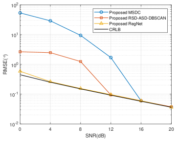
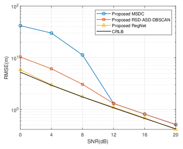
Figure 7: RMSE versus SNR, (a) DOA estimation, (b) range estimation.

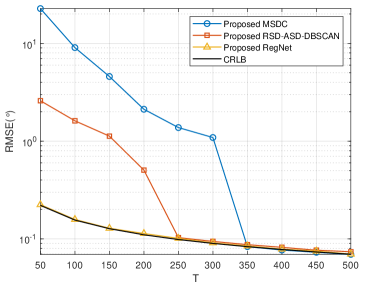
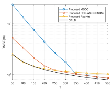
Figure 8: RMSE versus the number of snapshots $T$, (a) DOA estimation, (b) range estimation.

Fig.7 plots the RMSE of DOA and range estimations versus SNR for the proposed three methods and CRLB with $T=50$. By combining (a) and (b), it is clear that the proposed RegNet outperforms other methods, its DOA and range estimation accuracy can both achieve the CRLB at $\rm{SNR}=4dB$. Then based on the performance of DOA estimation and distance estimation respectively, compared to the two clustering-based methods, the proposed RegNet has a significant DOA estimation performance advantage in the medium-to-low SNR region, while the distance estimation accuracy shows improvement across all SNR regions. RSD-ASD-DBSCAN is a method with performance second only to the RegNet, its DOA estimation accuracy can achieve CRLB at $\rm{SNR}=12dB$, and its localization performance evidently outperforms MSDC especially in the medium-to-low SNR region. Finally, MSDC has a good localization performance with high SNR, it can achieve CRLB at $\rm{SNR}=16dB$ for DOA estimation, and its range estimation accuracy can keep pace with RSD-ASD-DBSCAN at $\rm{SNR}=12dB$.

Fig.8 illustrates the localization accuracy of the proposed methods versus the number of snapshots $T$ with $\rm{SNR}=5dB$. Similar to the trend of RMSE versus SNR, the proposed RegNet still has great advantages over other methods achieves CRLB in the low number of snapshots region. RSD-ASD-DBSCAN also performs significantly better than MSDC as $T<350$ and attains the CRLB of DOA estimation at $T=250$. But the different situation is when $T>250$, the range estimation accuracy of RSD-ASD-DBSCAN and MSDC can exceed that of RegNet and the difference will be larger with the increasing of $T$. Therefore, by combining Fig.7 and Fig.8, we can find the proposed RegNet has robust localization performance in the medium-to-low SNR and number of snapshots situations, while the proposed RSD-ASD-DBSCAN is more reliable with high SNR and $T$.

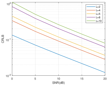
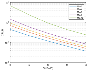
Figure 9: CRLB versus SNR, (a) grouped hybrid arrays with different $L$ and common $M_{s}=3$, (b) grouped hybrid arrays with different $M_{s}$ and common $L=5$.

As with the fixed array size $M$, the structure of grouped hybrid array depends on the number of groups $L$ and the number of antennas $M_{s}$ contained in each subarray. So in order to explore the impact of array structures on the localization performance, we plot the CRLB versus SNR for grouped hybrid arrays with different structures, and since the CRLB of DOA estimation and range estimation have similar trends, only the DOA estimation case is shown here. Firstly, in figure (a), the comparison is made between the grouped hybrid arrays with different $L$ and common $M_{s}$, we can see the grouped arrays with less number of groups have lower CRLB which mean they have potential to achieve more accurate localization results, and the CRLB for the arrays with $L=10$ and $L=2$ differ by almost an order of magnitude. Fig.9 (b) compares the CRLB of arrays with common $L$ and different $M_{s}$, it is clear that the increasing of $M_{s}$ will also cause the rising of CRLB. Therefore, when designing an grouped hybrid array, within the range of meeting the condition (7), we should minimize $L$ and $M_{s}$ as much as possible to achieve higher localization accuracy.

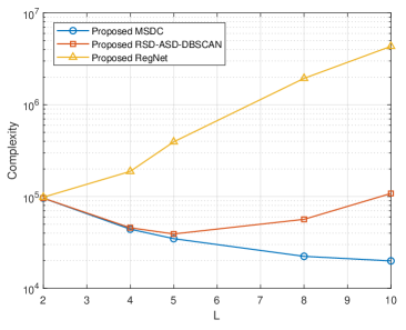
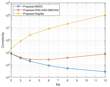
Figure 10: Computation complexity of the proposed methods, (a) complexity versus $L$ with $M_{s}=3$, (b) complexity versus $M_{s}$ with $L=5$.

Fig.10 depicts the computation complexity of the proposed methods versus $L$ and $M_{s}$. The specific complexity expressions are given in the Table I. Since the input size of the proposed RegNet is $LM_{s}$, and network size including depth and hidden layer size is strongly associated with the input size, the increasing of $L$ or $M_{s}$ will lead to the enlargement of RegNet size. So the complexity of RegNet increases apparently with the growth of $L$ and $M_{s}$, and is much higher than RSD-ASD-DBSCAN and MSDC for the unsupervised methods can save the computation spending of training stage. The sample number of the proposed RSD-ASD-DBSCAN also raises with the increasing of $L$ and $M_{s}$, its complexity exceeds that of MSDC at $L=4$ and $M_{s}=3$, and the difference becomes larger with the growth of $L$ and $M_{s}$.

VIII Conclusion

In this paper, we first proposed a grouped HAD structure for NF DOA estimation. By dividing the large-scale receive into several small-scale groups, the NF problem of estimating DOA within each group is viewed as a FF one. Then a candidate position set was generated by calibrating the estimation results of all the groups to a common reference point. Based on the distribution characters of the samples in the candidate position set, two low-complexity clustering-based methods, MSDC and RSD-ASD-DBSCAN, were proposed to solve phase ambiguity problem and locate the NF emitter. In order to further improve the localization accuracy, we proposed a high-resolution RegNet as well, which contains an MLNN for false solution elimination and a perceptron for angle fusion. Eventually, the CRLB of NF emitter localization for proposed grouped hybrid structure was derived as a performance benchmark for the proposed methods. The simulation results showed that the clustering-based methods can achieve the CRLB at high SNR region with extremely low complexity, while the proposed RegNet attains CRLB at much lower SNR level and has significantly performance improvement in the medium-to-low SNR regions.

Derivation of CRLB for NF Emitter localization via Proposed Grouped HAD Structure

Based on (68) we can get the Fisher information matrix (FIM) of the proposed grouped hybrid architecture as

$$\mathbf{F}=\begin{bmatrix}F_{\theta\theta}&F_{\theta r}\\ F_{r\theta}&F_{rr}\end{bmatrix},$$ (71)

where

$$F_{\beta_{i}\beta_{j}} ={\rm{tr}}\left\{\mathbf{R}^{-1}\frac{\partial\mathbf{R}}{\partial\beta_{i}}\mathbf{R}^{-1}\frac{\partial\mathbf{R}}{\partial\beta_{j}}\right\}$$ (72)

$$={\rm{tr}}\left\{\begin{bmatrix}\mathbf{R}_{1}^{-1}\frac{\partial\mathbf{R}_{1}}{\partial\beta_{i}}\mathbf{R}_{1}^{-1}\frac{\partial\mathbf{R}_{1}}{\partial\beta_{j}}&&\\ &\ddots&\\ &&\mathbf{R}_{L}^{-1}\frac{\partial\mathbf{R}_{L}}{\partial\beta_{i}}\mathbf{R}_{L}^{-1}\frac{\partial\mathbf{R}_{L}}{\partial\beta_{j}}\end{bmatrix}\right\}$$

$$=\sum_{l=1}^{L}{\rm{tr}}\left\{\mathbf{R}_{l}^{-1}\frac{\partial\mathbf{R}_{l}}{\partial\beta_{i}}\mathbf{R}_{l}^{-1}\frac{\partial\mathbf{R}_{l}}{\partial\beta_{j}}\right\}$$

$$=\sum_{l=1}^{L}F_{\beta_{i}\beta_{j}}^{(l)}$$

where $\bm{\beta}=[\theta,r]^{T}$, $1\leq i,j\leq 2$ and

$$F_{\beta_{i}\beta_{j}}^{(l)}={\rm{tr}}\left\{\mathbf{R}_{l}^{-1}\frac{\partial\mathbf{R}_{l}}{\partial\beta_{i}}\mathbf{R}_{l}^{-1}\frac{\partial\mathbf{R}_{l}}{\partial\beta_{j}}\right\}.$$ (73)

Then referring to (67), we can first attain two basic terms of $F_{\beta_{i}\beta_{j}}^{(l)}$

$$\frac{\partial\mathbf{R}_{l}}{\partial\theta}=\mathbf{W}_{l}^{H}\left(\dot{\mathbf{a}}_{l,\theta}\mathbf{a}_{l}^{H}+\mathbf{a}_{l}\dot{\mathbf{a}}^{H}_{l,\theta}\right)\mathbf{W}_{l},$$ (74)

$$\frac{\partial\mathbf{R}_{l}}{\partial r}=\mathbf{W}_{l}^{H}\left(\dot{\mathbf{a}}_{l,r}\mathbf{a}_{l}^{H}+\mathbf{a}_{l}\dot{\mathbf{a}}^{H}_{l,r}\right)\mathbf{W}_{l},$$

where $\mathbf{a}_{l}=\mathbf{a}(\varphi_{l})$ and

$$\dot{\mathbf{a}}_{l,\theta}=\frac{\partial\mathbf{a}_{l}}{\partial\theta}=j\frac{2\pi d}{\lambda}\dot{\varphi}_{l,\theta}\mathbf{D}\mathbf{a}_{l},$$ (75)

$$\dot{\mathbf{a}}_{l,r}=\frac{\partial\mathbf{a}_{l}}{\partial r}=j\frac{2\pi d}{\lambda}\dot{\varphi}_{l,r}\mathbf{D}\mathbf{a}_{l},$$

where $\mathbf{D}={\rm{diag}}\{0,1,\cdots,GM_{s}-1\}$, and

$$\dot{\varphi}_{l,\theta}=\frac{\partial\varphi_{l}}{\partial\theta}=\frac{r^{3}\cos\theta-\Delta d_{l}r^{2}\sin\theta\cos\theta}{(\sqrt{r^{2}-2\Delta d_{l}r\sin\theta+\Delta d_{l}^{2}})^{3}},$$ (76)

$$\dot{\varphi}_{l,r}=\frac{\partial\varphi_{l}}{\partial r}=\frac{\Delta d_{l}r\cos^{2}\theta}{(\sqrt{r^{2}-2\Delta d_{l}r\sin\theta+\Delta d_{l}^{2}})^{3}}.$$

So (74) can be further expressed by

$$\frac{\partial\mathbf{R}_{l}}{\partial\theta}=j\frac{2\pi d}{\lambda}\dot{\varphi}_{l,\theta}\mathbf{W}_{l}^{H}\left(\mathbf{D}\mathbf{a}_{l}\mathbf{a}_{l}^{H}-\mathbf{a}_{l}\mathbf{a}_{l}^{H}\mathbf{D}\right)\mathbf{W}_{l},$$ (77)

$$\frac{\partial\mathbf{R}_{l}}{\partial r}=j\frac{2\pi d}{\lambda}\dot{\varphi}_{l,r}\mathbf{W}_{l}^{H}\left(\mathbf{D}\mathbf{a}_{l}\mathbf{a}_{l}^{H}-\mathbf{a}_{l}\mathbf{a}_{l}^{H}\mathbf{D}\right)\mathbf{W}_{l},$$

and by substituting it into (73) we can get

$$F_{\theta\theta}^{(l)}=\dot{\varphi}_{l,\theta}^{2}\mu^{2}{\rm{tr}}\left\{\left[\mathbf{R}_{l}^{-1}\mathbf{W}_{l}^{H}\left(\mathbf{D}\mathbf{a}_{l}\mathbf{a}_{l}^{H}-\mathbf{a}_{l}\mathbf{a}_{l}^{H}\mathbf{D}\right)\mathbf{W}_{l}\right]^{2}\right\}$$ (78a)

$$F_{rr}^{(l)}=\dot{\varphi}_{l,r}^{2}\mu^{2}{\rm{tr}}\left\{\left[\mathbf{R}_{l}^{-1}\mathbf{W}_{l}^{H}\left(\mathbf{D}\mathbf{a}_{l}\mathbf{a}_{l}^{H}-\mathbf{a}_{l}\mathbf{a}_{l}^{H}\mathbf{D}\right)\mathbf{W}_{l}\right]^{2}\right\}$$ (78b)

$$F_{\theta r}^{(l)}=\dot{\varphi}_{l,\theta}\dot{\varphi}_{l,r}\mu^{2}{\rm{tr}}\left\{\left[\mathbf{R}_{l}^{-1}\mathbf{W}_{l}^{H}\left(\mathbf{D}\mathbf{a}_{l}\mathbf{a}_{l}^{H}-\mathbf{a}_{l}\mathbf{a}_{l}^{H}\mathbf{D}\right)\mathbf{W}_{l}\right]^{2}\right\}$$ (78c)

$$F_{r\theta}^{(l)}=\dot{\varphi}_{l,r}\dot{\varphi}_{l,\theta}\mu^{2}{\rm{tr}}\left\{\left[\mathbf{R}_{l}^{-1}\mathbf{W}_{l}^{H}\left(\mathbf{D}\mathbf{a}_{l}\mathbf{a}_{l}^{H}-\mathbf{a}_{l}\mathbf{a}_{l}^{H}\mathbf{D}\right)\mathbf{W}_{l}\right]^{2}\right\}$$ (78d)

where $\mu=j\frac{2\pi d}{\lambda}$. Then referring to the CRLB of the sub-connected hybrid structure derived in [24], and substituting (76) into the above equation, the expressions of $F_{\beta_{i}\beta_{j}}^{(l)}$ are further expressed by

$$F_{\theta\theta}^{(l)}=\frac{\mu^{2}r^{4}\cos^{2}\theta(r-\Delta d_{l}\sin\theta)^{2}\Xi_{l}}{(r^{2}-2\Delta d_{l}r\sin\theta+\Delta d_{l}^{2})^{3}},$$ (79a)

$$F_{rr}^{(l)}=\frac{\mu^{2}\Delta d_{l}^{2}r^{2}\cos^{4}\theta\Xi_{l}}{(r^{2}-2\Delta d_{l}r\sin\theta+\Delta d_{l}^{2})^{3}},$$ (79b)

$$F_{\theta r}^{(l)}=F_{r\theta}^{(l)}=\frac{\mu^{2}\Delta d_{l}r^{3}\cos^{3}\theta(r-\Delta d_{l}\sin\theta)\Xi_{l}}{(r^{2}-2\Delta d_{l}r\sin\theta+\Delta d_{l}^{2})^{3}},$$ (79c)

where $\Xi_{l}$ is given by (80), $\gamma=\sigma_{s}^{2}/\sigma_{v}^{2}$, and

$$\Xi_{l}=-\frac{2\gamma^{2}}{d^{2}M_{s}(M_{s}+\gamma G\lVert\Gamma_{l}\rVert^{2})^{2}}\left[\frac{\lVert\Gamma_{l}\rVert^{4}M_{s}^{2}G^{2}(G^{2}-1)(M_{s}+\gamma G\lVert\Gamma_{l}\rVert^{2})}{12}+M_{s}G\lVert\Gamma_{l}\rVert^{2}\lVert\eta_{l}\rVert^{2}+M_{s}G^{2}\Re(\Gamma_{l}^{2}\eta_{l})\right]$$ (80)

$$\Gamma_{l}=\sum_{m_{s}=1}^{M_{s}}e^{j\frac{2\pi d}{\lambda}(m_{s}-1)\varphi_{l}}=\frac{1-e^{j\frac{2\pi d}{\lambda}M_{s}\varphi_{l}}}{1-e^{j\frac{2\pi d}{\lambda}\varphi_{l}}},$$ (81a)

$$\eta_{l}=\sum_{m_{s}=1}^{M_{s}}(m_{s}-1)e^{-j\frac{2\pi d}{\lambda}(m_{s}-1)\varphi_{l}}.$$ (81b)

As CRLB is the inversion of FIM, given the number of snapshots $T$, then the CRLB of the proposed grouped hybrid architecture is given by

$${\rm{CRLB}}=\frac{1}{T}\mathbf{F}^{-1}=\begin{bmatrix}{\rm{CRLB}}_{\theta}&\\ &{\rm{CRLB}}_{r}\end{bmatrix},$$ (82)

from (71) and (72) we can get

$${\rm{CRLB}}_{\theta} =\frac{F_{rr}}{T(F_{\theta\theta}F_{rr}-F_{\theta r}F_{r\theta})}$$ (83)

$$=\frac{\sum_{l=1}^{L}F_{rr}^{(l)}}{T\left[\sum_{l=1}^{L}F_{\theta\theta}^{(l)}\sum_{l=1}^{L}F_{rr}^{(l)}-(\sum_{l=1}^{L}F_{\theta r}^{(l)})^{2}\right]},$$

and

$${\rm{CRLB}}_{r} =\frac{F_{\theta\theta}}{T(F_{\theta\theta}F_{rr}-F_{\theta r}F_{r\theta})}$$ (84)

$$=\frac{\sum_{l=1}^{L}F_{\theta\theta}^{(l)}}{T\left[\sum_{l=1}^{L}F_{\theta\theta}^{(l)}\sum_{l=1}^{L}F_{rr}^{(l)}-(\sum_{l=1}^{L}F_{\theta r}^{(l)})^{2}\right]}.$$

References

- [1] Y. Zhao, L. Dai, J. Zhang, C. Huang, Y. Liu, Y. Yuan, A. A. Hammadi, A. Elzanaty, A. Chen, B. Zheng et al., “6G near-field technologies white paper.” FuTURE Forum, 2024.
- [2] Z. Zhou, X. Gao, J. Fang, and Z. Chen, “Spherical wave channel and analysis for large linear array in LoS conditions,” in 2015 IEEE Globecom Workshops (GC Wkshps). IEEE, 2015, pp. 1–6.
- [3] X. Yin, S. Wang, N. Zhang, and B. Ai, “Scatterer localization using large-scale antenna arrays based on a spherical wave-front parametric model,” IEEE Trans. Wireless Commun., vol. 16, no. 10, pp. 6543–6556, 2017.
- [4] M. Cui and L. Dai, “Channel estimation for extremely large-scale MIMO: Far-field or near-field?” IEEE Trans. Commun., vol. 70, no. 4, pp. 2663–2677, 2022.
- [5] X. Zhang, H. Zhang, and Y. C. Eldar, “Near-field sparse channel representation and estimation in 6G wireless communications,” IEEE Trans. Commun., 2023.
- [6] T. Mao, J. Chen, Q. Wang, C. Han, Z. Wang, and G. K. Karagiannidis, “Waveform design for joint sensing and communications in millimeter-wave and low terahertz bands,” IEEE Trans. Commun., vol. 70, no. 10, pp. 7023–7039, 2022.
- [7] R. Liu, M. Jian, D. Chen, X. Lin, Y. Cheng, W. Cheng, and S. Chen, “Integrated sensing and communication based outdoor multi-target detection, tracking, and localization in practical 5G networks,” Intelligent and Converged Networks, vol. 4, no. 3, pp. 261–272, 2023.
- [8] Z. Zhang, Y. Liu, Z. Wang, X. Mu, and J. Chen, “Physical layer security in near-field communications,” IEEE Trans. Veh. Technol., 2024.
- [9] Y.-D. Huang and M. Barkat, “Near-field multiple source localization by passive sensor array,” IEEE Trans. Antennas Propag., vol. 39, no. 7, pp. 968–975, 1991.
- [10] J. Liang and D. Liu, “Passive localization of mixed near-field and far-field sources using two-stage MUSIC algorithm,” IEEE Trans. Signal Process., vol. 58, no. 1, pp. 108–120, 2009.
- [11] X. Zhang, W. Chen, W. Zheng, Z. Xia, and Y. Wang, “Localization of near-field sources: A reduced-dimension MUSIC algorithm,” IEEE Commun. Lett., vol. 22, no. 7, pp. 1422–1425, 2018.
- [12] R. N. Challa and S. Shamsunder, “High-order subspace-based algorithms for passive localization of near-field sources,” in Conference record of the twenty-ninth asilomar conference on signals, systems and computers, vol. 2. IEEE, 1995, pp. 777–781.
- [13] E. Grosicki, K. Abed-Meraim, and Y. Hua, “A weighted linear prediction method for near-field source localization,” IEEE Trans. Signal Process., vol. 53, no. 10, pp. 3651–3660, 2005.
- [14] W. Liu, J. Xin, W. Zuo, J. Li, N. Zheng, and A. Sano, “Deep learning based localization of near-field sources with exact spherical wavefront model,” in 2019 27th European Signal Processing Conference (EUSIPCO). IEEE, 2019, pp. 1–5.
- [15] Y. Cao, T. Lv, Z. Lin, P. Huang, and F. Lin, “Complex resnet aided doa estimation for near-field MIMO systems,” IEEE Trans. Veh. Technol., vol. 69, no. 10, pp. 11 139–11 151, 2020.
- [16] S. Jang and C. Lee, “Neural network-aided near-field channel estimation for hybrid beamforming systems,” IEEE Trans. Commun., 2024.
- [17] X. Su, P. Hu, Z. Liu, T. Liu, B. Peng, and X. Li, “Mixed near-field and far-field source localization based on convolution neural networks via symmetric nested array,” IEEE Trans. Veh. Technol., vol. 70, no. 8, pp. 7908–7920, 2021.
- [18] M. Qi, W. Ren, and H. Xiang, “Separation of mixed near-field and far-field sources and doa estimation based on deep learning,” in 2023 IEEE 15th International Conference on Advanced Infocomm Technology (ICAIT). IEEE, 2023, pp. 226–233.
- [19] X. Zhang, A. F. Molisch, and S.-Y. Kung, “Variable-phase-shift-based rf-baseband codesign for mimo antenna selection,” IEEE Trans. Signal Process., vol. 53, no. 11, pp. 4091–4103, 2005.
- [20] S. S. Ioushua and Y. C. Eldar, “A family of hybrid analog–digital beamforming methods for massive mimo systems,” IEEE Trans. Signal Process., vol. 67, no. 12, pp. 3243–3257, 2019.
- [21] V. V. Ratnam, A. F. Molisch, O. Y. Bursalioglu, and H. C. Papadopoulos, “Hybrid beamforming with selection for multiuser massive mimo systems,” IEEE Trans. Signal Process., vol. 66, no. 15, pp. 4105–4120, 2018.
- [22] F. Sohrabi and W. Yu, “Hybrid digital and analog beamforming design for large-scale antenna arrays,” IEEE J. Sel. Topics Signal Process., vol. 10, no. 3, pp. 501–513, 2016.
- [23] S.-F. Chuang, W.-R. Wu, and Y.-T. Liu, “High-resolution aoa estimation for hybrid antenna arrays,” IEEE Trans. Antennas Propag., vol. 63, no. 7, pp. 2955–2968, 2015.
- [24] F. Shu, Y. Qin, T. Liu, L. Gui, Y. Zhang, J. Li, and Z. Han, “Low-complexity and high-resolution DOA estimation for hybrid analog and digital massive MIMO receive array,” IEEE Trans. Commun., vol. 66, no. 6, pp. 2487–2501, 2018.
- [25] R. Zhang, B. Shim, and W. Wu, “Direction-of-arrival estimation for large antenna arrays with hybrid analog and digital architectures,” IEEE Trans. Signal Process., vol. 70, pp. 72–88, 2021.
- [26] A. Barabell, “Improving the resolution performance of eigenstructure-based direction-finding algorithms,” in ICASSP’83. IEEE International Conference on Acoustics, Speech, and Signal Processing, vol. 8. IEEE, 1983, pp. 336–339.
- [27] M. Ester, H.-P. Kriegel, J. Sander, X. Xu et al., “A density-based algorithm for discovering clusters in large spatial databases with noise,” in kdd, vol. 96, no. 34, 1996, pp. 226–231.
- [28] C. Cortes and V. Vapnik, “Support-vector networks,” Machine learning, vol. 20, pp. 273–297, 1995.
- [29] C. M. Bishop, Neural networks for pattern recognition. Oxford university press, 1995.
- [30] D. E. Rumelhart, G. E. Hinton, and R. J. Williams, “Learning representations by back-propagating errors,” nature, vol. 323, no. 6088, pp. 533–536, 1986.
- [31] B. W. Silverman, Density estimation for statistics and data analysis. Routledge, 2018.