Physical networks become what they learn

Abstract

Physical networks can develop diverse responses, or functions, by design, evolution or learning. We focus on electrical networks of nodes connected by resistive edges. Such networks can learn by adapting edge conductances to lower a cost function that penalizes deviations from a desired response. The network must also satisfy Kirchhoff’s law, balancing currents at nodes, or, equivalently, minimizing total power dissipation by adjusting node voltages. The adaptation is thus a double optimization process, in which a cost function is minimized with respect to conductances, while dissipated power is minimized with respect to node voltages. Here we study how this physical adaptation couples the cost landscape, the landscape of the cost function in the high-dimensional space of edge conductances, to the physical landscape, the dissipated power in the high-dimensional space of node voltages. We show how adaptation links the physical and cost Hessian matrices, suggesting that the physical response of networks to perturbations holds significant information about the functions to which they are adapted.

Electrical resistor networks must satisfy Kirchhoff’s laws when boundary conditions such as current or voltage inputs are imposed. Equivalently they must minimize dissipated power [1]. This minimization produces specific voltages at network nodes, and can be understood as a form of physical computation [2, 3, 4]. Electrical networks that use local rules to adapt computations they perform [5, 6, 7, 8, 9, 10, 11, 12] can be made in the laboratory using, e.g., contrastive learning procedures [13, 14, 15, 16, 17], and are arguably the simplest systems where learning emerges from local dynamical processes. In these systems, learning and adaptation leave physical imprints: soft modes aligned with learned tasks [18, 19, 20] appear in the dynamics. This behavior suggests an emergent connection between the physical behavior of a network and the computations it performs, or functions to which it is adapted.

Here we show that in electrical networks that adapt to satisfy constraints, the Hessian in the physical landscape, characterizing curvatures around the minimized power in the space of node voltages, is directly related to the Hessian in the cost landscape, characterizing curvatures around the minimized cost function in the space of adaptive edge conductances. As in deep neural networks [21, 22, 23, 24], the cost Hessian has high eigenmodes (directions of high curvature in the cost landscape) corresponding to learned tasks. We show that, after transformation by an adjacency matrix encoding the physical structure of the network, these modes lie largely in the space spanned by the low eigenmodes of the physical network. We give an example where the lowest eigenmode of the physical Hessian is related directly to the highest eigenmode of the cost Hessian.

Calculating the cost Hessian requires knowing the task. In contrast, the physical Hessian is a network property. Thus, the physical Hessian can give insight into an adaptive network’s function without applying inputs, defining input and output nodes, or knowing the task. The connection between the cost and physical Hessians is therefore valuable for understanding learning.

Physical and cost Hessians – Consider a linear electrical resistor network, with $N$ nodes indexed by $\mathbf{a}$, carrying voltages $\mathbf{V_{a}}$ collected into a voltage vector $\mathbf{V}$. Nodes are connected by $N_{e}$ edges indexed by $i$, of conductance $\kappa_{i}$. We use bold fonts for dynamical physical degrees of freedom (physical DOF; node voltages), and Greek/calligraphic font for adaptive degrees of freedom (adaptive DOF; edge conductances). Electrical resistor networks minimize total power dissipation. Because our networks are linear, the dissipated power is

$$\begin{aligned} \mathbf{P}=\frac{1}{2}\mathbf{V}^{T}\mathbf{H}\mathbf{V}\end{aligned},$$ (1)

with a symmetric physical $N\times N$ Hessian matrix,

$$\mathbf{H_{ab}}=\frac{\partial^{2}\mathbf{P}}{\partial\mathbf{V_{a}}\partial\mathbf{V_{b}}}\equiv 2\left[\mathbf{\Delta}^{T}\kappa\mathbf{\Delta}\right]_{\mathbf{ab}},$$ (2)

where $\mathbf{a,b}$ index the $N$ nodes; $i$, $j$ index the $N_{e}$ edges; $\kappa$ is a diagonal matrix of edge conductances with $\kappa_{ij}=\kappa_{i}\,\delta_{ij}$; and the notation $[\cdots]_{\mathbf{ab}}$ indicates a component of the matrix contained within the parentheses. $\mathbf{\Delta}$ is an adjacency matrix specifying the network geometry, with $\mathbf{\Delta}_{j\mathbf{a}}=1,0,-1$ depending on whether edge $j$ is incoming, disconnected, or outgoing to node $\mathbf{a}$, with arbitrarily assigned edge directions. For the sake of clarity, we discuss this form of the physical Hessian without ground nodes. For more information, specifically about the ground nodes, see SI Note 1. Thus the physical Hessian $\mathbf{H}$ depends on the adaptive conductances $\kappa_{i}$.

When external currents $\mathbf{I_{a}}$, collected into a vector $\mathbf{I}$, are applied to network nodes, the network minimizes the free state power dissipation, i.e., total power subject to the inputs: $\mathbf{P}^{F}=\mathbf{V}^{T}(\frac{1}{2}\mathbf{H}\mathbf{V}-\mathbf{I})$. The minimum of the free state power is achieved by the free state voltage values:

$$\mathbf{V}^{F}(\kappa;\mathbf{I})=\mathbf{H}^{-1}(\kappa)\,\mathbf{I}.$$ (3)

In this context, learning a target output response amounts to adapting conductances to satisfy an output constraint on the free state response $c(\mathbf{V}^{F})=0$ [25]. We can quantify this objective in terms of a scalar cost function $C$ often taken to be the square of the constraint:

$$C\equiv\frac{1}{2}c^{2}\,.$$ (4)

The process of modifying the adaptive conductances to minimize the cost function $C$ is called supervised learning when training examples with labels are provided. The cost then measures how well the network reproduces labels, or, more generally, the desired response.

Learning terminates when the system reaches a minimum of the cost function, so that both the cost function and its gradient with respect to $\kappa_{i}$ vanish. The cost landscape is then locally described to lowest nonvanishing order by the cost Hessian, an $N_{e}\times N_{e}$ matrix

$$\mathcal{H}_{ij}\equiv\frac{\partial^{2}C}{\partial\kappa_{i}\partial\kappa_{j}}.$$ (5)

Recall that $N_{e}$ is the number of network edges or adaptive parameters. The cost Hessian is studied in machine learning approaches to improve gradient descent [26]. If a model is well-trained for $n_{T}$ tasks, e.g., it has low training error, then the cost Hessian has $n_{T}$ non-vanishing eigenvalues, while the rest of the eigenvalues vanish [21, 22, 23]. The associated eigenmodes characterize the decision boundary in classification tasks [24].

Relation between the physical and cost Hessians– The physical and cost Hessians have different dimensions and different units, but we will see that they are nevertheless related. We can rewrite the cost Hessian as

$$\mathcal{H}_{ij}=\frac{\partial^{2}C}{\partial\kappa_{i}\partial\kappa_{j}}=\frac{\partial c}{\partial\kappa_{i}}\frac{\partial c}{\partial\kappa_{j}}+c\frac{\partial^{2}c}{\partial\kappa_{i}\partial\kappa_{j}}\equiv\mathcal{H}_{ij}^{\mathrm{sat}}+\mathcal{H}_{ij}^{\mathrm{dyn}}\,,$$ (6)

a sum of the satisfied term $\mathcal{H}_{ij}^{\mathrm{sat}}\equiv\frac{\partial c}{\partial\kappa_{i}}\frac{\partial c}{\partial\kappa_{j}}$ and the dynamic term $\mathcal{H}_{ij}^{\mathrm{dyn}}\equiv c\frac{\partial^{2}c}{\partial\kappa_{i}\partial\kappa_{j}}$. $\mathcal{H}_{ij}^{\mathrm{dyn}}$ vanishes identically when the network achieves the desired output ($c=0$). Further, from (6) we see that when there is only one constraint, $\mathcal{H}_{ij}^{\mathrm{sat}}$ is a rank-1 matrix–it is an outer product of a vector $g_{i}\equiv\frac{\partial c}{\partial\kappa_{i}}$ with itself. Clearly, $g_{i}$ is proportional to an eigenmode of $\mathcal{H}_{ij}^{\mathrm{sat}}$. The situation with multiple constraints is explained in SI Note 2.

Assume there is a single constraint and that it is satisfied, so that $\mathcal{H}^{\mathrm{dyn}}$ vanishes. To relate the physical and cost Hessians, recall that the constraint $c(\mathbf{V}^{F})$ is an explicit function of the free state response, so that

$$\begin{aligned} g_{i}=\frac{dc}{d\mathbf{V}^{F}}\cdot\frac{\partial\mathbf{V}^{F}}{\partial\kappa_{i}}=-\frac{dc}{d\mathbf{V}^{F}}\cdot\mathbf{H}^{-1}\frac{\partial\mathbf{H}}{\partial\kappa_{i}}\mathbf{H}^{-1}\mathbf{I}\end{aligned}.$$ (7)

where by $\frac{dc}{d\mathbf{V}^{F}}$ we mean the gradient with respect to $\mathbf{V}^{F}$, and we used (3) along with the standard formula for the derivative of the inverse of a matrix. Finally, applying the $\kappa_{i}$ derivative to the physical Hessian in Eq. 2 we arrive at

$$g_{i}=-2(\frac{dc}{d\mathbf{V}^{F}}\cdot\mathbf{H}^{-1}\mathbf{\Delta}_{i}^{T})(\mathbf{\Delta}_{i}\mathbf{H}^{-1}\mathbf{I})\,,$$ (8)

where by ${\bf\Delta}_{i}$ we mean the the ith row of ${\bf\Delta}$. So ${\bf\Delta}_{i}$ is a vector of length $N$ whose entries are 1 for the node that edge $i$ enters, $-1$ for the node it leaves, and $0$ for the other nodes. So we find schematically that

$$\mathcal{H}_{ij}^{\mathrm{sat}}=g_{i}g_{j}\sim\mathbf{H}^{-4}.$$ (9)

Eq. 9 encodes a remarkable connection between the physical and cost landscapes when the constraint is satisfied so that the cost is minimized: the curvature around the solution in the cost landscape is directly related to the curvature around the minimum of the physical power landscape. This connection arises because the power must be minimized to satisfy Kirchhoff’s law at every node while the cost is decreased; as a result, the two landscapes become entangled in their respective spaces.

Again, note that the satisfied cost Hessian in (9) is an outer product of the vector $g_{i}$ (the gradient of the constraint with respect to $\kappa_{i}$) with itself. Thus, if there is a single constraint the cost Hessian will be rank $1$, with one non-vanishing eigenvalue and corresponding eigenmode $g_{i}$ associated with the learned task. Moreover, from the definition of the cost function Eq. 4,

$$\frac{\partial C}{\partial\kappa_{i}}=cg_{i}$$ (10)

Evidently, as the cost vanishes, the cost gradient is proportional to the nontrivial eigenmode of the cost Hessian. The analysis thus far can be generalized to any physical system that minimizes a Lyapunov function in the linear response limit, including mechanical networks that minimize energy or free energy, or flow and electrical networks that minimize dissipated power or, more generally, their “co-content” [27, 6].

To clarify how physical and cost Hessian eigenmodes relate to each other, we first rotate to the natural coordinates of the physical Hessian:

$$H=\bm{v}^{T}\Lambda\bm{v}$$ (11)

$$\mathbf{i}\equiv\bm{v}\mathbf{I}\quad;\quad\mathbf{o}\equiv\bm{v}\frac{dc}{d\mathbf{V}^{F}}\,.$$

Here $\bm{v}$ is a matrix whose rows are eigenmodes of the physical Hessian, $\Lambda$ is a diagonal matrix of the associated eigenvalues $\mathbf{\lambda}>0$, and $\mathbf{i},\mathbf{o}$ are input current vector and the gradient of the constraint rotated to the physical Hessian frame of reference.

In this coordinate system

$$\begin{aligned} g_{i}=-2\sum_{\mathbf{ab}}\Big{(}\frac{\mathbf{i}}{\lambda}\Big{)}_{\mathbf{a}}\Big{(}\frac{\mathbf{o}}{\lambda}\Big{)}_{\mathbf{b}}(\mathbf{\Delta}_{i}\bm{v}_{\mathbf{a}}^{T})(\mathbf{\Delta}_{i}\bm{v}_{\mathbf{b}}^{T})\end{aligned}.$$ (12)

The vector $(\frac{\mathbf{i}}{\lambda})_{\mathbf{a}}$ is the input current in the direction of eigenmode $\bm{v}_{\mathbf{a}}$, divided by the associated eigenvalue $\lambda_{a}$; similarly for $(\frac{\mathbf{o}}{\lambda})_{\mathbf{a}}$. The quantity $\mathbf{\Delta}_{i}{\bm{v}}^{T}_{\mathbf{a}}$ is the voltage difference across the $i$th edge for the $\mathbf{a}$th eigenvector.

We previously showed that if there is a single satisfied constraint the physical Hessian tends to develop a soft mode with a small eigenvalue $\lambda_{1}$ [20]. If this eigenvalue is much smaller than the rest, we can approximate Eq. 12 by a single term, just as we discussed above for the cost Hessian of a network trained to achieve a single constraint

$$\begin{aligned} g_{i}^{\mathrm{Approx}}=-2\frac{\mathbf{i}_{1}\mathbf{o}_{1}}{\lambda_{1}^{2}}(\mathbf{\Delta}_{i}\bm{v}_{1}^{T})^{2}\end{aligned}.$$ (13)

So, in this case, we find that the stiff mode of the cost Hessian $\mathcal{H}$ has components proportional to the squared differences of the node voltages belonging to the soft mode of the physical Hessian $\bf{H}$. Note that $\bf{H}$ can be estimated from physical responses alone [28], with no knowledge about the constraints the system was required to satisfy. This implies that without knowing $\mathbf{i},\mathbf{o}$ we can obtain a good approximation of the stiff mode of $\mathcal{H}^{\mathrm{sat}}$. In other words, one does not need to specify the task – to know the constraints or cost function–in order to learn which edges most strongly affect the error in a trained network.

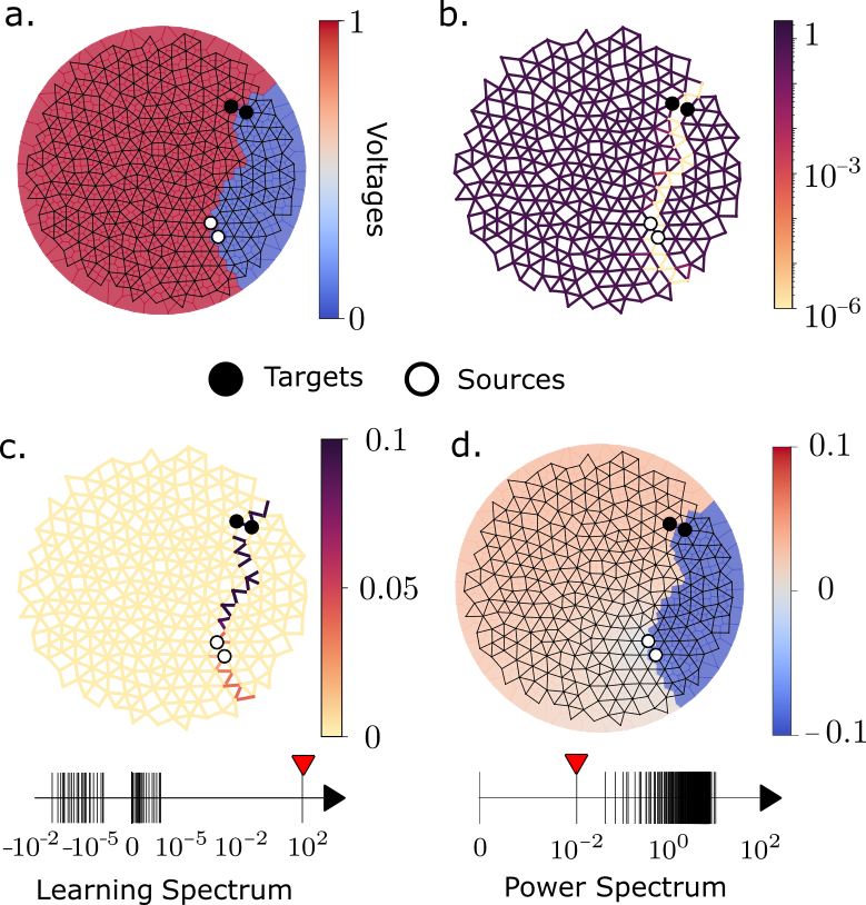
Figure 1: Linear electrical resistor networks have correlated modes in the physical and cost spaces, illustrated for a simple extreme case, in which the voltage drop between two output nodes (black) is constrained to be equal to the voltage drop between two input nodes (white). (a) The voltage response of the network, where the color interpolates between the node voltages. The response is partitioned into two sectors, with high uniform voltage and low uniform voltage, respectively. (b) The edge conductances; the network develops a crack of low conductance. c) The stiff mode of the cost Hessian picks out the edges in the crack. d) The soft mode of the physical Hessian reflects the voltage response and complements the stiff mode of the learning Hessian.

An illustrative example is shown in Fig. 1 for an electrical network trained so that a voltage drop applied between the two white input nodes yields an equal voltage drop between the two black output nodes (for training details task see SI Note 3). We see that the voltage response in the network partitions it into high voltage and low voltage sectors (Fig. 1a), separated by a crack of low conductance (Fig. 1b).Furthermore, the stiff mode of the cost Hessian is spatially localized to the low-conductance crack (Fig. 1c); if these conductances are varied from their low values, the cost increases strongly. Note that the lowest non-trivial eigenmode of the physical Hessian (Fig. 1d), captures the response of the network to the input, even though no information regarding the input or output is required to identify this mode. Moreover, applying the voltage difference operator $\mathbf{\Delta}_{i}$ to this soft mode, it is clear that $(\Delta_{i}v_{1})^{2}$ is also spatially localized to the crack, so this mode reflects the key edges associated with the stiff mode of the cost Hessian. The stiff mode of the cost Hessian corresponds to the boundary between two sectors identified by the physical Hessian; these sectors and the boundary between are consistent with topological data analysis [29, 30], showing a direct connection between our Hessian analysis and persistent homology in this case.

Once the single constraint is satisfied, we can approximate the cost Hessian according to Eq. 9 as:

$$\begin{aligned} \mathcal{H}_{ij}^{\mathrm{Approx}}\approx 4\frac{(\mathbf{i}_{1}\mathbf{o}_{1})^{2}}{\lambda_{1}^{4}}(\mathbf{\Delta}_{i}\bm{v}^{T}_{1})^{2}(\mathbf{\Delta}_{j}\bm{v}^{T}_{1})^{2}\end{aligned}.$$ (14)

This cost Hessian is the outer product of a vector and hence has rank 1. So its trace is equal to its single non-zero eigenvalue: $\lambda^{\mathcal{L}}_{1}={\rm Tr}(\mathcal{H}^{\mathrm{Approx}})$. Performing the trace relates the stiff eigenvalue of the cost Hessian to the soft eigenvalue of the physical Hessian:

$$\begin{aligned} \lambda_{1}^{\mathcal{L}}=4\sum_{i}g_{i}^{2}\approx\frac{(\mathbf{i}_{1}\mathbf{o}_{1})^{2}}{\lambda_{1}^{4}}\sum_{i}(\mathbf{\Delta}_{i}\bm{v}^{T}_{1})^{4}\propto\lambda_{1}^{-4}\end{aligned}.$$ (15)

To test these results numerically, we trained resistor networks for $1000$ examples of tasks similar to that in Fig. 1. The results are summarized in SI Note 4 and Fig. S1.

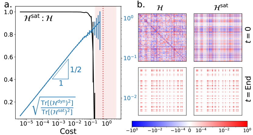
Figure 2: Cost Hessian as cost $C$ decreases during the double optimization process for a task requiring a given voltage drop between two output nodes in response to a current applied between two input nodes. (a) As predicted, the cost Hessian is well captured by $\mathcal{H}^{\mathrm{sat}}$ (black curve), when the cost is lowered compared to the lowest physical eigenvalue $C\lesssim\lambda_{1}^{-2}$. The vertical red line is the median of $\lambda_{1}^{-2}$ and the middle 2 quartiles of the range are shown as the red shaded region. The ratio of dynamic to satisfied cost Hessians (blue curve) scales as $\sqrt{C}$, as predicted. (b) Comparison of the full and satisfied cost Hessians before and after the double optimization process.

Dynamical Hessian relations – We now examine how the two Hessians are related during the double optimization process, not just at the end when the constraints have been satisfied. Returning to Eq. 6, we find that (details in SI Note 5):

$$\mathcal{H}_{ij}= \mathcal{H}_{ij}^{\mathrm{sat}}+\mathcal{H}_{ij}^{\mathrm{dyn}}$$ (16)

$$= g_{i}g_{j}+4cL_{i}M_{ij}R_{j}+4cL_{j}M_{ji}R_{i}$$

$$+4cR_{i}R_{j}\sum_{\mathbf{ab}}({\bf\Delta}_{i}{\bf H}^{-1})_{\mathbf{a}}\frac{\partial^{2}c}{\partial{\bf V}^{F}_{\mathbf{a}}\partial{\bf V}^{F}_{\mathbf{b}}}({\bf H}^{-1}{\bf\Delta}^{T}_{j})_{\mathbf{b}}$$

where we defined $L_{i}\equiv\frac{dc}{d{\bf v}^{F}}\cdot{\bf H}^{-1}{\bf\Delta}_{i}^{T}$, $R_{i}\equiv{\bf\Delta}_{i}{\bf H}^{-1}{\bf I}$, and $M_{ij}\equiv{\bf\Delta}_{i}{\bf H}^{-1}{\bf\Delta}_{j}^{T}$. The last three terms arise from $\mathcal{H}_{ij}^{\mathrm{dyn}}$. Recall that $\mathcal{H}_{ij}^{\mathrm{sat}}\sim\mathbf{H}^{-4}$. The first two terms in $\mathcal{H}_{ij}^{\mathrm{Dyn}}$ scale as $c\mathbf{H}^{-3}\sim\sqrt{C}\mathbf{H}^{-3}$, while the last term scales as $c\mathbf{H}^{-4}\sim\sqrt{C}\mathbf{H}^{-4}$. For systems with a linear constraint, like the electrical networks that we study, the last term vanishes because $\frac{\partial^{2}c}{\partial{\bf V}^{F}_{a}\partial{\bf V}^{F}_{b}}=0$. In that case, $\mathcal{H}^{\mathrm{sat}}$ dominates the cost Hessian, $\mathrm{Tr}[(\mathcal{H}^{\mathrm{sat}})^{2}]\gg\mathrm{Tr}[(\mathcal{H}^{\mathrm{dyn}})^{2}]$, once the error is reduced below a scale set by the lowest eigenvalue of the physical Hessian, $C\ll\lambda_{1}^{-2}$. For systems with a nonlinear constraint, $\mathcal{H}^{\mathrm{sat}}$ still dominates, at least after the error is small enough, i.e., $C\ll 1$. The change of the physical Hessian $\bf{H}$ during learning is proportional to the cost function gradient. Thus, the physical Hessian $\mathbf{H}$ becomes nearly constant at low $C$.

We confirm these results numerically in Fig. 2 for networks with a linear constraint. We trained $300$ networks to produce desired output voltage drops in response to applied input currents, and calculated $\mathcal{H}^{\mathrm{sat}}$ and $\mathcal{H}^{\mathrm{dyn}}$ during the learning process. Fig. 2(a) shows that the cost Hessian $\mathcal{H}$ is well approximated by $\mathcal{H}^{\mathrm{sat}}$, so that the normalized double dot product $\mathcal{H}^{\mathrm{sat}}:\mathcal{H}\equiv\frac{\mathrm{Tr}[\mathcal{H}^{\mathrm{sat}}\mathcal{H}]}{\sqrt{\mathrm{Tr}[(\mathcal{H}^{\mathrm{sat}})^{2}]}\sqrt{\mathrm{Tr}[\mathcal{H}^{2}]}}$ approaches $1$ (black) when the cost drops far enough below a threshold $\lambda_{1}^{-2}$ set by the lowest physical Hessian eigenvalue, $\lambda_{1}$. Additionally, Fig. 2(a) shows that the ratio of the dynamic and satisfied terms, $\sqrt{\mathrm{Tr}[(\mathcal{H}^{\mathrm{dyn}})^{2}]/\mathrm{Tr}[(\mathcal{H}^{\mathrm{sat}})^{2}]}$, scales as the square root of the error $C$ (blue), as predicted. In Fig. 2b, we show the cost Hessian for one specific network before and after the double optimization process. Initially $\mathcal{H}^{\mathrm{sat}}$ approximates the cost Hessian poorly, but afterwards it captures it well, with the same sparse, low-rank features.

Discussion – We derived relations between the physical and cost Hessians for electrical resistor networks as they adapt to perform tasks. Networks that satisfy one constraint have a cost Hessian of rank 1; we generalize in the Supplemental Material to show that networks that satisfy $n_{T}$ constraints have rank $n_{T}$ cost Hessians. We showed in examples that the high eigenmodes of the satisfied cost Hessian include network edges that adapt to satisfy the constraints. We showed further that these high eigenmodes of the satisfied cost Hessian are related to low eigenmodes of the physical Hessian. When the system creates a single low physical eigenmode well-separated by a gap from the higher eigenmodes, we found that the high cost Hessian eigenmode is closely related to the low physical Hessian eigenmode. In this case, many features of the satisfied constraint can be discovered physically without knowing the constraint a priori. Even when the low eigenmodes of the physical Hessian are not separated by a gap from the rest, the connection between the Hessians suggests strategies for learning about stiff cost Hessian eigenmodes from physical information only [31]. We related the physical and cost Hessians for linear electrical resistor networks, but similar relations hold in the linear response regime for any physical network that has adapted or evolved to minimize a scalar Lyapunov function. In other words, we are showing that, in a sense, physical networks become what they learn.

Our approach applies to adaptive mechanical systems [32, 33, 34, 35, 36], including evolved proteins, where correlations between physical structure and function [37, 38, 39, 40, 41, 42] appear in regions highly conserved over evolutionary times, suggesting their functional importance [38, 43]. For example, such conserved regions in proteins have been associated with slow collective dynamical modes–which correspond to low eigenmodes of the physical Hessian [44]. Because our approach links the physical and cost Hessians for each system, it can give insight into individual systems as well as for an ensemble of solutions, as in a protein family, perhaps shedding light on idiosyncratic features that play functional roles [45].

More broadly, circuit networks in the brain display structures that are conserved among individuals and even species [46]. In many cases these conserved structures can be understood as evolved or learned adaptations to the environment or to tasks, for example, in the sensory circuits supporting vision [47, 48, 49], audition [50, 51], and olfaction [52, 53]. However, differences between individuals are also functionally important, e.g., for encoding specific memories [54, 55]. Our findings, by linking structure and function in individual networks, may help to explain how conserved network adaptations can be accompanied by substantial individual variations [56, 57].

We thank Eric Rouviere, Pratik Chaudhari, Benjamin Machta, Pankaj Mehta, and Arvind Murugan for insightful discussions. This work was supported by DOE Basic Energy Sciences through grant DE-SC0020963 (MS,MG,FM,AJL), the UPenn NSF NRT DGE-2152205 (FM) and the Simons Foundation through Investigator grant #327939 to AJL. VB and MS were also supported by NIH CRCNS grant 1R01MH125544-01 and NSF grant CISE 2212519. This work was completed at the Aspen Center for Physics (NSF grant PHY-2210452).

References

- [1] Sri Krishna Vadlamani, Tianyao Patrick Xiao, and Eli Yablonovitch. Physics successfully implements lagrange multiplier optimization. Proceedings of the National Academy of Sciences, 117(43):26639–26650, 2020.
- [2] Rolf Landauer. Computation: A fundamental physical view. Physica Scripta, 35(1):88, 1987.
- [3] Gualtiero Piccinini. Physical computation: A mechanistic account. OUP Oxford, 2015.
- [4] Herbert Jaeger, Beatriz Noheda, and Wilfred G Van Der Wiel. Toward a formal theory for computing machines made out of whatever physics offers. Nature communications, 14(1):4911, 2023.
- [5] Benjamin Scellier and Yoshua Bengio. Equilibrium propagation: Bridging the gap between energy-based models and backpropagation. Frontiers in computational neuroscience, 11:24, 2017.
- [6] Jack Kendall, Ross Pantone, Kalpana Manickavasagam, Yoshua Bengio, and Benjamin Scellier. Training end-to-end analog neural networks with equilibrium propagation. arXiv preprint arXiv:2006.01981, 2020.
- [7] Menachem Stern, Daniel Hexner, Jason W Rocks, and Andrea J Liu. Supervised learning in physical networks: From machine learning to learning machines. Physical Review X, 11(2):021045, 2021.
- [8] Corinna Kaspar, Bart Jan Ravoo, Wilfred G van der Wiel, Seraphine V Wegner, and Wolfram HP Pernice. The rise of intelligent matter. Nature, 594(7863):345–355, 2021.
- [9] Menachem Stern and Arvind Murugan. Learning without neurons in physical systems. Annual Review of Condensed Matter Physics, 14(1):417–441, 2023.
- [10] Victor Lopez-Pastor and Florian Marquardt. Self-learning machines based on hamiltonian echo backpropagation. Physical Review X, 13(3):031020, 2023.
- [11] Vidyesh Rao Anisetti, Benjamin Scellier, and Jennifer M Schwarz. Learning by non-interfering feedback chemical signaling in physical networks. Physical Review Research, 5(2):023024, 2023.
- [12] Vidyesh Rao Anisetti, Ananth Kandala, Benjamin Scellier, and JM Schwarz. Frequency propagation: Multimechanism learning in nonlinear physical networks. Neural Computation, 36(4):596–620, 2024.
- [13] Sam Dillavou, Menachem Stern, Andrea J Liu, and Douglas J Durian. Demonstration of decentralized physics-driven learning. Physical Review Applied, 18(1):014040, 2022.
- [14] Jacob F. Wycoff, Sam Dillavou, Menachem Stern, Andrea J. Liu, and Douglas J. Durian. Desynchronous learning in a physics-driven learning network. The Journal of Chemical Physics, 156(14):144903, 2022.
- [15] Menachem Stern, Sam Dillavou, Marc Z Miskin, Douglas J Durian, and Andrea J Liu. Physical learning beyond the quasistatic limit. Physical Review Research, 4(2):L022037, 2022.
- [16] Sam Dillavou, Benjamin D Beyer, Menachem Stern, Marc Z Miskin, Andrea J Liu, and Douglas J Durian. Machine learning without a processor: Emergent learning in a nonlinear electronic metamaterial. arXiv preprint arXiv:2311.00537, 2023.
- [17] Menachem Stern, Sam Dillavou, Dinesh Jayaraman, Douglas J Durian, and Andrea J Liu. Training self-learning circuits for power-efficient solutions. APL Machine Learning, 2(1), 2024.
- [18] Benjamin B Machta, Ricky Chachra, Mark K Transtrum, and James P Sethna. Parameter space compression underlies emergent theories and predictive models. Science, 342(6158):604–607, 2013.
- [19] Vidyesh Rao Anisetti, Ananth Kandala, and JM Schwarz. Emergent learning in physical systems as feedback-based aging in a glassy landscape. arXiv preprint arXiv:2309.04382, 2023.
- [20] Menachem Stern, Andrea J Liu, and Vijay Balasubramanian. Physical effects of learning. Physical Review E, 109(2):024311, 2024.
- [21] Levent Sagun, Leon Bottou, and Yann LeCun. Eigenvalues of the hessian in deep learning: Singularity and beyond. arXiv preprint arXiv:1611.07476, 2016.
- [22] Levent Sagun, Utku Evci, V Ugur Guney, Yann Dauphin, and Leon Bottou. Empirical analysis of the hessian of over-parametrized neural networks. arXiv preprint arXiv:1706.04454, 2017.
- [23] Mingwei Wei and David J Schwab. How noise affects the hessian spectrum in overparameterized neural networks. arXiv preprint arXiv:1910.00195, 2019.
- [24] Mahalakshmi Sabanayagam, Freya Behrens, Urte Adomaityte, and Anna Dawid. Unveiling the hessian’s connection to the decision boundary. arXiv preprint arXiv:2306.07104, 2023.
- [25] Pankaj Mehta, Marin Bukov, Ching-Hao Wang, Alexandre GR Day, Clint Richardson, Charles K Fisher, and David J Schwab. A high-bias, low-variance introduction to machine learning for physicists. Physics reports, 2019.
- [26] Yann N Dauphin, Razvan Pascanu, Caglar Gulcehre, Kyunghyun Cho, Surya Ganguli, and Yoshua Bengio. Identifying and attacking the saddle point problem in high-dimensional non-convex optimization. In Z. Ghahramani, M. Welling, C. Cortes, N. Lawrence, and K. Q. Weinberger, editors, Advances in Neural Information Processing Systems, volume 27. Curran Associates, Inc., 2014.
- [27] Mauro Parodi and Marco Storace. Linear and nonlinear circuits: Basic & advanced concepts, volume 1. Springer, 2018.
- [28] Ke Chen, Wouter G Ellenbroek, Zexin Zhang, Daniel TN Chen, Peter J Yunker, Silke Henkes, Carolina Brito, Olivier Dauchot, Wim Van Saarloos, Andrea J Liu, et al. Low-frequency vibrations of soft colloidal glasses. Physical review letters, 105(2):025501, 2010.
- [29] Jason W Rocks, Andrea J Liu, and Eleni Katifori. Revealing structure-function relationships in functional flow networks via persistent homology. Physical Review Research, 2(3):033234, 2020.
- [30] Jason W Rocks, Andrea J Liu, and Eleni Katifori. Hidden topological structure of flow network functionality. Physical Review Letters, 126(2):028102, 2021.
- [31] Marcelo Guzman, Felipe Martins, and Andrea J Liu. Imprints of learned solutions in adaptive resistor networks. In prep.
- [32] Nidhi Pashine, Daniel Hexner, Andrea J Liu, and Sidney R Nagel. Directed aging, memory, and nature’s greed. Science Advances, 5(12):eaax4215, 2019.
- [33] Menachem Stern, Chukwunonso Arinze, Leron Perez, Stephanie E. Palmer, and Arvind Murugan. Supervised learning through physical changes in a mechanical system. Proceedings of the National Academy of Sciences, 117(26):14843–14850, 2020.
- [34] Chukwunonso Arinze, Menachem Stern, Sidney R. Nagel, and Arvind Murugan. Learning to self-fold at a bifurcation. Phys. Rev. E, 107:025001, Feb 2023.
- [35] Lauren E Altman, Menachem Stern, Andrea J Liu, and Douglas J Durian. Experimental demonstration of coupled learning in elastic networks. arXiv preprint arXiv:2311.00170, 2023.
- [36] Tie Mei and Chang Qing Chen. In-memory mechanical computing. Nature Communications, 14(1):5204, 2023.
- [37] Najeeb Halabi, Olivier Rivoire, Stanislas Leibler, and Rama Ranganathan. Protein sectors: evolutionary units of three-dimensional structure. Cell, 138(4):774–786, 2009.
- [38] Tiberiu Teşileanu, Lucy J Colwell, and Stanislas Leibler. Protein sectors: statistical coupling analysis versus conservation. PLoS computational biology, 11(2):e1004091, 2015.
- [39] Arjun S Raman, K Ian White, and Rama Ranganathan. Origins of allostery and evolvability in proteins: a case study. Cell, 166(2):468–480, 2016.
- [40] Michael R Mitchell, Tsvi Tlusty, and Stanislas Leibler. Strain analysis of protein structures and low dimensionality of mechanical allosteric couplings. Proceedings of the National Academy of Sciences, 113(40):E5847–E5855, 2016.
- [41] Tsvi Tlusty, Albert Libchaber, and Jean-Pierre Eckmann. Physical model of the genotype-to-phenotype map of proteins. Physical Review X, 7(2):021037, 2017.
- [42] Eric Rouviere, Rama Ranganathan, and Olivier Rivoire. Emergence of single-versus multi-state allostery. PRX Life, 1(2):023004, 2023.
- [43] Victor H Salinas and Rama Ranganathan. Coevolution-based inference of amino acid interactions underlying protein function. elife, 7:e34300, 2018.
- [44] Kabir Husain and Arvind Murugan. Physical constraints on epistasis. Molecular Biology and Evolution, 37(10):2865–2874, 2020.
- [45] Martin J Falk, Jiayi Wu, Ayanna Matthews, Vedant Sachdeva, Nidhi Pashine, Margaret L Gardel, Sidney R Nagel, and Arvind Murugan. Learning to learn by using nonequilibrium training protocols for adaptable materials. Proceedings of the National Academy of Sciences, 120(27):e2219558120, 2023.
- [46] Ricardo Olivares, Juan Montiel, and Francisco Aboitiz. Species differences and similarities in the fine structure of the mammalian corpus callosum. Brain Behavior and Evolution, 57(2):98–105, 2001.
- [47] Charles P Ratliff, Bart G Borghuis, Yen-Hong Kao, Peter Sterling, and Vijay Balasubramanian. Retina is structured to process an excess of darkness in natural scenes. Proceedings of the National Academy of Sciences, 107(40):17368–17373, 2010.
- [48] Patrick Garrigan, Charles P Ratliff, Jennifer M Klein, Peter Sterling, David H Brainard, and Vijay Balasubramanian. Design of a trichromatic cone array. PLoS computational biology, 6(2):e1000677, 2010.
- [49] Ann M Hermundstad, John J Briguglio, Mary M Conte, Jonathan D Victor, Vijay Balasubramanian, and Gašper Tkačik. Variance predicts salience in central sensory processing. Elife, 3:e03722, 2014.
- [50] Michael S Lewicki. Efficient coding of natural sounds. Nature neuroscience, 5(4):356–363, 2002.
- [51] Evan C Smith and Michael S Lewicki. Efficient auditory coding. Nature, 439(7079):978–982, 2006.
- [52] Tiberiu Teşileanu, Simona Cocco, Remi Monasson, and Vijay Balasubramanian. Adaptation of olfactory receptor abundances for efficient coding. Elife, 8:e39279, 2019.
- [53] Kamesh Krishnamurthy, Ann M Hermundstad, Thierry Mora, Aleksandra M Walczak, and Vijay Balasubramanian. Disorder and the neural representation of complex odors. Frontiers in Computational Neuroscience, 16:917786, 2022.
- [54] Edward K Vogel and Maro G Machizawa. Neural activity predicts individual differences in visual working memory capacity. Nature, 428(6984):748–751, 2004.
- [55] Lisa Feldman Barrett, Michele M Tugade, and Randall W Engle. Individual differences in working memory capacity and dual-process theories of the mind. Psychological bulletin, 130(4):553, 2004.
- [56] Romke Rouw and H Steven Scholte. Neural basis of individual differences in synesthetic experiences. Journal of Neuroscience, 30(18):6205–6213, 2010.
- [57] Svetlana V Shinkareva, Vicente L Malave, Marcel Adam Just, and Tom M Mitchell. Exploring commonalities across participants in the neural representation of objects. Human brain mapping, 33(6):1375–1383, 2012.