Benchmarking Spectral Graph Neural Networks:
A Comprehensive Study on Effectiveness and Efficiency
Abstract
With the recent advancements in graph neural networks (GNNs), spectral GNNs have received increasing popularity by virtue of their specialty in capturing graph signals in the frequency domain, demonstrating promising capability in specific tasks. However, few systematic studies have been conducted to assess their spectral characteristics. This emerging family of models also varies in terms of design and settings, leading to difficulties in comparing their performance and deciding on the suitable model for specific scenarios, especially for large-scale tasks. In this work, we extensively benchmark spectral GNNs with a focus on the frequency perspective. We analyze and categorize over 30 GNNs with 27 corresponding filters. Then, we implement these spectral models within a unified framework with dedicated graph computations and efficient training schemes. Thorough experiments are conducted on the spectral models with inclusive metrics on effectiveness and efficiency, offering practical guidelines on evaluating and selecting spectral GNNs with desirable performance. Our implementation enables application on larger graphs with comparable performance and less overhead, which is available at: https://github.com/gdmnl/Spectral-GNN-Benchmark.
1 Introduction
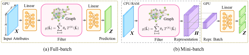
Graph neural networks (GNNs) have emerged as powerful tools in a wide range of graph understanding tasks. Spectral GNNs denote a specialized set of GNN designs that are based on spectral graph theory and apply graph signal filters in the spectral domain [1, 2, 3, 4]. Benefiting from diverse and adaptive spectral expressions, these models have garnered exceptional utility under both homophily and heterophily [5, 6], and in real-world scenarios such as multivariate time-series forecasting [7, 8] and point cloud processing [9, 10]. Particularly, spectral operations are feasible with a denser parameter space and less computational overhead while preserving expressiveness and efficacy, alleviating the conventional bottleneck of GNNs and rendering these models ideal for large-scale tasks. Figure 1 illustrates the basic concept of fitting spectral filters to different GNN training pipelines.
Existing Evaluations of Spectral GNNs.
The spectral domain of graphs has long been incorporated into graph learning tasks [11, 12]. We present a detailed review of related GNN surveys and benchmarks in Appendix C. Although a handful of classic spectral models have been included in previous benchmarks [13, 14], most of them lack specificity in considering and assessing characteristics from a spectral perspective. With the bloom of spectral GNNs in the last few years, we find that existing evaluations are particularly limited compared to recent research progress in various aspects.:
-
•
Advance in Spectral Interpretation: Latest studies have revealed the general relationship between spectral and spatial operations, where many classic and popular GNN designs have been shown to have corresponding spectral formations [15, 16, 17]. This new equivalence calls for interpreting and evaluating these models in the spectral domain.
-
•
Varied Implementations and Evaluations: Existing spectral GNNs vary greatly in non-spectral designs such as data processing, graph computation, and network architecture. These ancillary properties are less relevant to their spectral expressiveness. However, their diverse implementations affect the model performance and complicate the fair comparison of different spectral filters.
-
•
Limited Efficient Computation: As depicted in Figure 1, spectral GNNs are known for achieving favorable expressiveness with efficient and scalable designs. A line of recent works proposes dedicated algorithms for spectral computation [18, 19, 20, 21]. While other spectral filters are conceptually applicable to such enhancements, they are never implemented nor evaluated.
Our Contribution.
In this study, we are hence motivated to benchmark GNNs specifically in the spectral domain, presenting theoretical and empirical view of spectral filters within a unified framework. The scope of our evaluation covers a wide range of GNNs with spectral interpretations. By deriving and classifying proposed filters, we show that the majority of existing spectral models can be divided into three categories, exhibiting distinct capabilities and performance.
We offer dedicated implementation of these filters under the same framework, integrated with advanced data processing, network architecture, and scalable computation techniques. Based on our taxonomy and implementation, we conduct experimental comparison on performance including expressiveness, efficacy, efficiency, and scalability. Compared to previous GNN evaluations, we highlight the following specialties of this work:
-
•
Unified Framework: We offer an open-source, plug-and-play collection for spectral models and filters. The framework realizes unified and efficient implementations covering a variety of spectral GNN designs. Reproducible pipelines are included for training and evaluating the provided models.
-
•
Spectral-oriented Design: Our spectral framework is designed in a spectral-oriented manner independent to spatial operations. Such implementation ensures that most filters are easily adaptable to a wide range of model-level options on transformation, architecture, and learning schemes. In this way, spectral GNNs can be constructed on-demand from various choices of modules and configurations offering different precision, speed, and memory performances.
-
•
Comprehensive and Fair Evaluation: We provide extensive study on the effectiveness and efficiency of spectral filters across various model architectures and learning schemes under our framework. Particularly, most filters are applicable to graphs beyond million-scale, which has never been achieved before. We analyze the spectral properties of the filters and conclude practical guidelines for designing and utilizing spectral models as well as open questions for future research.
The key takeaways of our benchmark study characterizing effectiveness and efficiency of diverse types of spectral GNNs are summarized as follows:
-
•
All three types of filters are able to achieve satisfactory performance on homophilous graphs, while variable filters and filter bank models excel under heterophily. As there is no optimal single solution for all cases, comprehensive consideration of model capability and expense is required when choosing a suitable filter for learning distinct graph signals.
-
•
Filters with fixed parameters are the most efficient design for both full-batch and mini-batch training schemes. Variable feature transformation and additional graph propagation increase memory overhead and model learning time, respectively. The trade-off between efficacy and efficiency is critical for model applications, especially on large graphs.
-
•
Spectral models exhibit dissimilar effectiveness on nodes of high and low degrees under different graph conditions, which extends the presumption in previous studies. The bias also affects overall model prediction and may motivate dedicated filter designs to further enhance accuracy.
2 Formulations for Spectral GNN Paradigms
In this section, we first provide the general notations of spectral GNNs highlighting the polynomial approximation for the consideration of its predominant utility in real-world graph learning. Based on the formulation, we categorize polynomial filters into three types according to their parameterization schemes, which are summarized in Table 1 and introduced in respective subsections. A detailed list of filters and models is presented in Table 5 with analysis in Appendix B.
Graph Notation.
An undirected graph is denoted as with nodes and edges. The adjacency matrix without and with self-loops are and , respectively. The normalized adjacency matrix is , where is the self-looped diagonal degree matrix and is the normalization coefficient [18, 22]. The Laplacian matrix is defined as , while its normalized counterpart is . The attributed graph is associated with a node attribute matrix , carrying an -dimensional attribute vector for each node. Summary of primary symbols and notations used in the paper can be found in Table 4.
Spatial Graph Convolution.
The spatial interpretation understands GNN message-passing procedure as two stages, namely propagation and transformation. Propagation describes the process of applying graph matrix to the node representation as , inside which the aggregation operator characterizes the process of aggregating graph information. The other stage of transformation updates the representation with learnable weights.
From the view of network architecture, iterative GNNs incorporate the two stages in an alternative fashion: and . Applying such spatial convolution of iterations leads to a receptive field of hops on the graph. In contrast, decoupled models possess separated stages and can be formulated by , where are pre- and post-transformations performed by learnable weights, respectively.
Spectral Graph Convolution.
Graph spectral theory looks into the the eigen-decomposition of Laplacian , where graph spectrum is the diagonal matrix of eigenvalues , and is the matrix consisting of eigenvectors. For simplicity, here we present by considering the attribute vector as the input graph signal. GNNs adopting spectral convolution can be generally expressed as:
| (1) |
where is the frequency response, i.e., spectral filter, and denotes the diagonal matrix when applied to the graph spectrum. Eq. 1 can be understood by three consecutive stages: the Fourier transform upon the input signal , the modulation based on graph information , and lastly the inverse Fourier transform to the output .
In practice, directly acquiring eigen-decomposition is prohibitive for graph-scale matrices. Hence, it is common to utilize reduction in the form of -order polynomial approximation with regard to as an approximate filter . Such polynomial estimation is satisfactory for arbitrary smooth signals, while more complicated filters such as rational functions are required under signal discontinuity [23, 24]. Nonetheless, computing graph-scale matrix inverse for rational filters is impractical, which also leads to polynomial reduction in realistic implementations as elaborated in Appendix B.
Relation between spatial and spectral convolutions.
We examine the general case where the -order filter is derived from an arbitrary polynomial basis . Each term is parameterized by , which can either be a scalar or a matrix. Now the spectral convolution Eq. 1 is approximated by the polynomial filter with respect to basis :
| (2) |
A line of studies have revealed the relationship between spatial and spectral convolutions in the context of GNN learning [2, 25, 16, 17]. Without loss of generality, the spectral filter defined in Eq. 2 can be written as a polynomial based on as by expanding and substituting , which corresponds to the spatial convolution . In other words, the polynomial spectral filters can be achieved by a series of recurrent graph propagations. When the spatial and spectral orders align with each other, we have . We further discuss the architectural difference and respective complexity in Appendix A.
| Category | Models |
| Fixed Filter | GCN [2], SGC [26], gfNN [27], GZoom [28], S2GC [29], GLP [30], APPNP [31], GCNII [32], GDC [33], DGC [34], AGP [18], GRAND+ [19] |
| Variable Filter | GIN [35], AKGNN [36], DAGNN [37], GPRGNN [25], ARMAGNN [38], ChebNet [4], ChebNetII [20], HornerGCN/ClenshawGCN [39], BernNet [40], LegendreNet [41], JacobiConv [5], FavardGNN/OptBasisGNN [42] |
| Filter Bank | AdaGNN [43], FBGNN(I/II) [44], ACMGNN(I/II) [45], FAGCN [46], G2CN [47], GNN-LF/HF [48], FiGURe [49] |
2.1 Fixed Filter GNN
For spectral GNNs with polynomial filters in Eq. 2, the basis and the parameter jointly determine the actual response to graph signals, and consequently dominate the model performance [5]. It is pivotal for designing spectral GNNs to choose the basis and parameter that are suitable for the task. We thereby categorize polynomial spectral GNNs based on the acquisition schemes of bases and parameters into three types, as respectively introduced in the following subsections.
For the first type of spectral GNNs, the basis and parameters are both constant during learning, resulting in fixed filters . In practice, these filters are usually predefined simple schemes such as monomial or PPR summation. Below we give an example of the classic APPNP model and its filter:
Personalized PageRank (PPR).
The APPNP [31] model is computed by iteratively applying graph propagation to approximate the PPR calculation: , where denotes the decay coefficient. By selecting the basis , we name the spectral interpretation of APPNP as the PPR filter:
2.2 Variable Filter GNN
The second type of spectral GNN in our taxonomy also features a predetermined basis in Eq. 2. The series of parameters is variable, usually acquired through gradient descent during model training, leading to a variable filter . Compared to spectral GNNs with fixed filters, these models enjoy better capability, especially for fitting high-frequency signals and capturing non-local graph information. The choice of basis is the primary factor of the model performance on practical tasks [5, 42]. Below we present the representative Chebyshev filter.
Chebyshev.
ChebNet [4] utilizes the Chebyshev polynomial as basis. Each term in the polynomial is expressed in the recursive form based on the computation results and of previous hops. The Chebyshev spectral filter can be computed by:
2.3 Filter Bank GNN
Some studies argue that a single filter is limited in leveraging complex graph signals. Hence, spectral GNNs with filter bank arise as an advantageous approach to provide abundant information for learning. These models typically adopt multiple fixed or variable filters , each assigned with a filter weight parameter . When the number of filters is , their combination can be expressed as:
| (3) |
where denotes an arbitrary fusion function such as summation or concatenation. By this means, the filter bank is able to cover different channels, i.e., ranges of frequencies, to generate more comprehensive embeddings of the graph. The filter parameter can be either learned separately or along with GNN training, depending on the specific model implementation.
FiGURe.
3 Benchmark Design
Framework Implementation.
Based on the paradigm of spectral GNNs, we develop a unified framework oriented towards the invariable spectral filters in particular. As specified Section D.1, our implementation embraces the modular design principle, offering plug-and-play filter modules that can be seamlessly integrated into mainstream graph learning toolkits. It is also easily extendable to new filter designs, as only the spectral formulation described in Section 2 needs to be implemented. Then the filter enjoys a wide range of off-the-shelf blocks for building a complete GNN.
Tasks and Metrics.
We focus on the semi-supervised learning for node-classification task on a single graph, as it is the mainstream task for spectral GNNs. In particular, this task features some of the largest datasets available for graph learning, which is ideal for assessing the scalability of spectral models. We follow the dataset settings for using efficacy metrics including accuracy and ROC AUC. Efficiency with respect to both running speed and CPU/GPU memory usage is measured for each learning stage, including training, inference, and precomputation.
Datasets.
We comprehensively involve 22 representative datasets that are widely used in spectral GNN evaluation. We mainly categorize them from two aspects. In efficacy evaluations, we distinguish them into homophilous and heterophilous datasets, since performance under heterophily is the design motivation of many spectral filters. For experiments on efficiency, we separately investigate small-, medium-, and large-scale graphs, and focus on larger ones where the scalability issue of GNN models is more critical. Details of the benchmark datasets can be found in Section D.2.
Learning Schemes.
Figure 1 indicates that the spectral filter is invariable across different training schemes. Full-batch training loads all input data onto the GPU, which is the de facto scheme for most GNN models. In contrast, mini-batch scheme performs graph-related operations in a precomputation stage on CPU. Then, only the intermediate representations are loaded onto the GPU in batches during training, which prevents the memory footprint to be coupled with the graph size and enjoys better scalability. Our novel implementation enables the application of most filters to both schemes for fair and comprehensive comparison.
Model Architectures and Hyperparameters.
We unify the non-spectral aspects of architectures for all models in our evaluation, as an approach to provide comparable performance while enhancing scalability to larger graphs. This includes the same transformation operations, network depth and width, propagation hops, batch size, and training epochs among all models in the main experiment. For other hyperparameters not affecting efficiency, we perform individual hyperparameters tuning for each model and dataset. More elaboration and comparison among different architectural designs can be found in Section A.1, while details of hyperparameter search are elaborated in Section D.3.
4 Experimental Results
In this section, we present primary observations on the performance comparison among a total of 27 filters in three types. We also include our novel observations on the efficacy bias concerning nodes of different degrees. Complete experimental results are supplemented in Appendix E, while Appendix F and Appendix G present additional explorations on the spectral and degree-specific properties.
Type Filter cora citeseer pubmed flickr squirrel chameleon actor roman Fixed Identity 75.60±1.08 72.92±1.34 87.31±0.48 35.95±1.27 32.08±3.86 24.37±5.59 35.95±1.27 66.23±0.74 Linear 86.62±1.69 76.00±1.23 84.52±0.49 26.22±1.09 33.93±3.30 36.62±2.64 25.08±0.46 30.92±0.82 Impulse 86.21±1.53 74.79±1.03 83.02±0.74 26.48±0.83 34.21±3.71 35.23±2.20 27.00±1.30 27.90±0.59 Monomial 80.91±3.37 76.26±1.67 89.22±0.93 32.36±2.81 37.64±3.56 33.91±1.31 35.53±1.40 60.71±1.37 PPR 88.61±0.95 77.25±1.29 89.01±0.38 35.55±1.04 32.81±3.57 33.58±1.59 35.17±1.01 62.26±2.34 HK 88.06±0.99 77.10±0.89 89.11±0.63 37.33±1.48 32.64±4.06 34.28±1.50 37.53±1.25 65.60±0.92 Gaussian 86.37±2.12 76.92±1.16 89.06±0.76 35.62±0.87 33.54±4.02 37.18±1.82 36.44±1.25 66.47±0.94 Variable Linear 87.08±1.46 76.00±1.14 85.04±0.75 27.49±1.12 36.39±4.25 37.32±1.85 25.56±1.22 40.05±6.02 Monomial 87.56±1.00 76.72±1.25 88.18±0.76 35.42±1.89 39.33±2.90 40.65±1.67 32.13±3.47 64.76±0.66 Horner 86.14±1.82 76.72±1.61 89.59±0.45 36.74±0.88 37.92±3.41 34.57±1.35 37.65±1.10 61.52±0.88 Chebyshev 86.67±1.09 76.37±1.62 89.68±0.49 36.09±1.30 29.83±4.04 38.86±3.36 32.68±1.29 62.64±1.79 Clenshaw 80.33±3.72 74.14±1.48 86.35±2.12 31.16±2.42 31.40±3.08 34.26±1.41 27.03±5.10 68.03±1.51 ChebInterp 86.57±1.14 72.52±6.76 89.28±0.45 34.67±1.64 30.62±5.36 34.30±1.72 32.27±2.89 70.54±1.64 Bernstein 69.76±2.10 61.97±1.20 84.61±0.61 33.47±1.01 36.18±3.06 36.01±2.29 33.07±1.30 57.24±1.97 Legendre 86.56±1.12 77.15±0.86 89.83±0.40 35.70±1.40 35.51±6.95 35.52±1.50 35.63±1.01 57.04±5.64 Jacobi 81.40±3.05 74.67±1.15 89.56±0.38 35.30±1.51 31.69±3.93 36.87±1.60 36.10±1.47 63.25±1.66 Favard 82.74±4.59 74.16±2.94 89.44±0.43 30.89±2.58 30.56±4.02 37.05±2.49 36.37±1.13 62.19±1.41 OptBasis 82.20±2.22 73.59±2.04 88.16±1.92 33.76±2.12 33.76±3.81 33.76±1.91 34.26±1.09 64.46±1.60 Bank AdaGNN 85.91±0.81 74.96±0.98 89.97±0.50 36.28±1.44 35.00±4.35 35.32±1.57 36.49±1.21 66.13±1.35 FBGNNI 86.84±0.95 75.02±1.03 88.98±0.38 33.54±0.93 35.96±2.21 37.88±2.77 33.88±0.42 67.26±1.78 FBGNNII 87.91±1.56 72.21±1.92 88.87±0.53 34.21±0.67 37.53±5.29 33.87±1.47 35.30±0.75 72.61±1.68 ACMGNNI 87.25±1.27 76.00±1.20 88.84±0.66 33.38±1.27 33.37±3.50 30.68±3.18 33.59±1.20 64.19±1.65 ACMGNNII 81.89±3.59 74.60±0.60 89.07±0.38 34.14±0.60 34.05±3.70 27.43±3.33 33.49±1.31 73.40±1.30 FAGNN 86.60±1.43 75.95±1.52 85.06±0.42 24.89±1.38 31.29±5.22 35.61±2.35 27.82±1.21 28.20±1.39 G2CN 87.99±1.25 76.64±1.18 88.33±0.48 33.21±1.35 38.03±2.97 35.72±2.28 33.72±0.99 58.08±1.49 GNN-LF/HF 85.93±1.40 76.98±0.89 88.53±1.82 37.22±1.27 35.84±2.91 34.12±1.63 36.49±1.55 64.02±1.23 FiGURe 87.45±1.98 76.32±1.37 87.75±0.34 31.71±3.06 40.34±3.19 36.94±2.36 31.76±4.50 60.13±0.96
4.1 Overall Effectiveness and Efficiency Performance
Both effectiveness and efficiency are important for GNN applications in practice. Our benchmark study aims to offer a comprehensive view considering both factors. Tables 2 and 3, along with Tables 8, 9, 10 and 11, include the results with regard to model efficacy and efficiency for full- and mini-batch training. Observations are based on the complete evaluation on all datasets.
Obs.#1: Filter effectiveness varies under conditions of heterophily and is relevant to different types of spectral designs. Graph heterophily affects the prediction performance of different filter types in distinctive manners, and no filter achieves dominant efficacy across all scenarios. On homophilous graphs, the accuracy gap among the three types is relatively marginal and mostly within the error interval. With proper settings, even conventional fixed filters can achieve superior performance, such as PPR and HK on cora and citeseer. However, fixed filters typically fail under heterophily, while more variable and complex designs retain higher performance, confirming their utility in addressing the heterophily issue of canonical GNNs. In most cases, full-batch and mini-batch training schemes do not diversify the model efficacy.
We associate the difference in performance with the design of filter parameterization. Models with fixed parameters are constrained to exploit low-frequency graph signals, which is shown to be beneficial only under homophily. In contrast, variable parameters offer a more flexible approach in approximating a wider range of the graph spectrum. This allows for dynamically learning filter weights based on the graph pattern, which is preferable for capturing and leveraging useful information in the frequency domain to produce a more comprehensive understanding of the graph.
Type Filter pokec products snap wiki Pre. Train Infer RAM GPU Pre. Train Infer RAM GPU Pre. Train Infer RAM GPU Pre. Train Infer RAM GPU Fixed Linear 8.45 6.52 6.23 6.61 0.48 19.5 1.56 10.3 21.6 1.75 27.3 10.5 8.30 20.8 0.63 206.5 11.4 6.80 57.5 0.94 Impulse 5.36 7.30 6.37 6.58 0.48 15.0 1.57 10.3 21.6 1.74 21.0 10.7 8.37 18.1 0.63 164.1 10.9 7.40 57.5 0.94 Monomial 5.22 7.24 6.53 6.59 0.48 15.5 1.55 10.4 21.6 1.76 21.9 11.1 8.70 18.0 0.61 172.6 11.5 6.40 57.4 0.93 PPR 5.68 6.86 6.33 6.60 0.45 15.8 1.55 10.6 21.6 1.35 20.3 10.4 8.43 18.1 0.61 166.6 11.1 5.97 57.4 0.94 HK 5.21 7.08 6.30 6.62 0.48 14.8 1.54 11.1 21.6 1.49 18.8 11.1 8.37 18.1 0.63 165.6 10.4 5.80 57.4 0.94 Gaussian 5.24 6.78 7.67 6.61 0.48 14.7 1.51 9.77 21.6 1.63 19.7 11.3 9.97 18.1 0.63 156.1 10.2 6.10 57.5 0.94 Variable Linear 5.66 12.5 15.6 11.8 1.19 16.6 2.31 16.2 25.9 2.06 26.5 17.0 22.4 70.3 4.87 175.4 15.8 17.1 109.0 10.8 Monomial 6.04 15.3 14.6 11.8 1.19 15.3 2.63 15.4 25.9 1.92 25.0 18.1 17.0 70.3 4.87 166.9 16.6 11.8 109.1 10.8 Horner 6.21 13.4 17.8 11.8 1.19 20.9 3.40 25.5 25.9 2.18 23.5 17.7 24.7 70.3 4.87 203.7 18.3 23.8 109.1 10.8 Chebyshev 7.12 13.6 12.0 12.3 1.19 24.1 3.21 17.6 27.3 2.19 26.3 16.1 15.4 70.5 4.87 198.6 16.9 16.2 114.5 10.8 Clenshaw 7.74 14.2 19.1 11.8 1.19 28.4 3.14 23.9 25.9 2.33 35.1 21.9 31.6 70.3 4.87 234.1 18.8 23.8 109.1 10.8 ChebInterp 7.34 125.6 77.0 12.3 1.19 23.5 35.2 102.1 27.3 2.26 35.2 461.2 108.6 70.5 4.87 239.9 628.5 78.2 114.5 10.8 Bernstein 26.4 15.5 15.2 13.4 1.59 99.7 3.27 20.6 30.7 2.42 100.0 22.4 44.3 71.0 5.25 1268.6 18.2 14.5 125.5 11.7 Legendre 7.50 15.6 12.9 11.8 1.19 22.5 2.97 15.0 25.9 2.04 32.1 19.1 15.9 70.3 4.87 205.8 16.7 11.0 109.1 10.8 Jacobi 8.99 15.3 14.4 11.8 1.19 23.3 3.03 15.7 25.9 2.15 42.8 18.7 19.8 70.3 4.87 203.6 16.5 12.8 109.1 10.8 OptBasis 35.1 14.1 13.9 11.9 1.19 87.2 3.15 17.9 25.9 2.41 269.1 21.3 18.7 70.5 4.87 477.9 16.1 11.3 109.1 10.8 Bank FAGNN 15.3 9.08 7.73 6.56 0.57 46.9 2.11 11.8 21.6 1.14 68.9 16.0 13.8 23.6 1.03 438.8 13.2 7.17 57.2 1.96 G2CN 28.2 8.63 6.57 6.57 0.57 81.9 2.08 11.0 21.5 0.92 91.0 14.0 10.1 23.6 1.03 827.7 14.6 8.00 57.2 1.96 GNN-LF/HF 12.5 8.33 6.83 7.36 0.57 38.0 2.02 11.3 23.8 1.36 52.7 14.8 11.0 21.8 1.03 385.5 13.2 7.33 59.7 1.96 FiGURe 46.6 26.4 26.6 37.1 3.52 145.2 5.69 35.6 84.6 5.71 175.1 39.7 40.4 230.8 14.5 1458.7 55.3 47.0 358.4 20.1
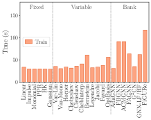
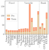
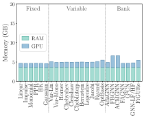
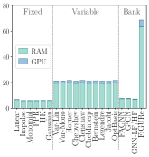
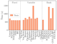
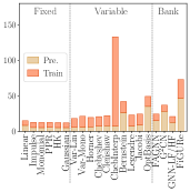
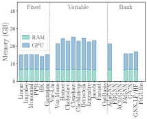
Obs.#2: Fixed filters achieve top-tier efficiency and scalability. For both full- and mini-batch training schemes, fixed-filter GNNs share similar and the best runtime and memory efficiency. Filter bank models consisting of fixed filters also exhibit comparable performance when the graph scale is small. Figure 2 illustrates a more in-depth breakdown of the time and memory footprints. We mainly observe two design factors that increase the model overhead. Firstly, variable transformations and subsequent operations come at the price of more computational resources. In the full-batch scheme, this leads to lower speed and higher GPU memory demand. Specifically, those with complex representation computations, including Favard, OptBasis, FBGNN, and ACMGNN, are among the models with prolonged training time and the worst memory scalability, incurring out-of-memory errors on large graphs. For mini-batch training, the cost is indicated by the increased RAM usage, since the model needs to store precomputation results compared to for fixed filters. Similarly, a filter bank design with filters demands up to times larger memory.
On the other hand, the second factor of additional propagations slows down learning but barely affects memory scalability. This can be inferred from ChebINterp and Bernstein filters, which possess more graph propagations than others. The design demonstrates significantly longer runtime, especially on larger graphs, where the graph-scale propagation becomes the speed bottleneck. However, their memory footprint is on par with fellow variable filters.
Obs.#3: An ideal spectral GNN necessitates comprehensive consideration of the efficacy-efficiency trade-off. Combining Sections 4.1 and 4.1, there is an evident trade-off between efficacy and efficiency among spectral models, where more challenging scenarios call for sophisticated designs but come with longer running times and higher memory requirements. We suggest the following practice as an effort to balance effectiveness and efficiency: when learning on simple and homophilous graphs, one can stick to fixed filters such as PPR for the best efficiency and comparable superb precision; for tasks under heterophily, it is recommended to carefully choose the suitable model for fitting the graph data and producing satisfying performance, while ensuring the time and memory overhead remain feasible in the given environment.
In terms of learning schemes, mini-batch training showcases preferable time and memory scalability compared to the full-batch scheme. As displayed in Figure 2, on medium-sized graphs, both schemes present the same level of overall running speed for most filters. However, on large datasets such as pokec, mini-batch learning is faster, as it saves the expensive graph propagation operation from iterative training. Moreover, it transfers the majority of memory load from GPU to RAM, which enables the employment of filters exceeding the GPU memory limit in the full-batch scheme. The GPU memory complexity independent from the graph scale is favorable for deploying spectral GNNs in a wider range of environments.
margin=2em,0em,skip=3pt
\subcaptionsetupmargin=1.5em,-2em,skip=-1pt
\subcaptionsetupmargin=2em,0em,skip=3pt
\subcaptionsetupmargin=1.5em,-2em,skip=-1pt
4.2 Degree-specific Effectiveness
Recent works reveal the node-wise performance difference of vanilla GNNs with respect to nodes of varying degree levels [50, 51, 52, 53, 54]. In this benchmark, we are motivated to offer preliminary investigation regarding the degree-specific performance of spectral GNNs, including the causing factors and impacts of the phenomenon. Corresponding evaluations are in Figure 3 and Appendix G.
Obs.#4: Degree-wise effectiveness varies under conditions of homophily and heterophily. Unlike previous investigations assuming homophily, Figure 3 displays the difference between prediction accuracy on high- and low-degree nodes extending to heterophilous datasets. It can be observed that most filters behave distinctively under these two conditions. On homophilous graphs, performance of high-degree nodes is generally on par with or higher than low-degree ones, which echoes earlier studies. From the spectral domain view, high-degree nodes are commonly located in clusters, which is more related to low frequency in graph spectrum and is favorable for homophilous GNNs.
Contrarily, the accuracy of high-degree nodes is usually significantly lower under heterophily. In this case, the hypothesis that higher degrees are naturally favored by GNNs no longer holds true. Although these nodes aggregate more information from the neighborhood, it is not essentially beneficial, and heterophilous connections may carry destructive bias and hinder the prediction. As a more precise amendment for the conclusion in prior works, we state that the degree-wise bias is more sensitive, but not necessarily beneficial, to high-degree nodes with regard to varying graph conditions.
margin=1em,0em,skip=2pt \subcaptionsetupmargin=2em,-2em

Obs.#5: Degree-wise bias is relevant to the overall effectiveness of filters. It is also notable in Figure 3 that the degree-specific difference is correlated with the test accuracy of models within each dataset. Filters adhering to Section 4.2 with greater bias achieve relatively better performance on roman. In comparison, filters such as Linear and Impulse fail to distinguish high- and low-degree nodes, and the test accuracy is lower. The observation suggests that GNNs tend to recognize and adapt to the majority of low-degree nodes in order to achieve higher performance on heterophilous graphs, although such a strategy sacrifices the performance of high-degree nodes.
5 Discussion and Open Question
In this study, we conduct extensive evaluations for spectral GNNs regarding both effectiveness and efficiency. We first provide thorough analysis of the spectral kernels in existing GNNs and categorize them by spectral designs. These filters are then implemented under a unified framework with plug-and-play modules and highly-efficient schemes. Comprehensive experiments are conducted to assess the model performance, with discussions covering heterophily, graph scales, spectral properties, and degree-wise bias. We highlight the large-scale experiments thanks to our scalable implementation. Our benchmark observations also identify several open questions worth further discussion and study towards better spectral GNNs:
-
•
How to improve spectral filters by balancing efficacy and efficiency? As demonstrated in Sections 4.1, 4.1 and 4.1, the most efficient fixed-filter models are only effective in a limited range of graphs, while more powerful variable and composed filters are far from optimized efficiency. As the scalability issue is notorious for GNNs in realistic applications, it is of practical interest to pursue designs enjoying both efficacy and efficiency. Our study is helpful in uncovering impact factors and bottlenecks of large-scale deployment, and underscores the potential of spectral GNNs for more scalable schemes.
-
•
How to address the degree-specific bias and enhance overall effectiveness? In Sections 4.2 and 4.2, we discover that the degree-wise difference is related with graph heterophily and affects model precision. As current endeavors mitigating the GNN bias largely assume homophily, it is promising to search for specialized schemes with accuracy improvement of both low- and high-degree nodes considering various graph conditions, which also benefits overall model performance.
References
- [1] Bruna, J., W. Zaremba, A. Szlam, et al. Spectral networks and locally connected networks on graphs. In 2nd International Conference on Learning Representations. 2014.
- [2] Kipf, T. N., M. Welling. Semi-supervised classification with graph convolutional networks. In International Conference on Learning Representations. 2017.
- [3] Atwood, J., D. Towsley. Diffusion-convolutional neural networks. In 29th Advances in Neural Information Processing Systems, pages 2001–2009. 2016.
- [4] Defferrard, M., X. Bresson, P. Vandergheynst. Convolutional neural networks on graphs with fast localized spectral filtering. Advances in neural information processing systems, 29, 2016.
- [5] Wang, X., M. Zhang. How powerful are spectral graph neural networks. In Proceedings of the 39th International Conference on Machine Learning, vol. 162, pages 23341–23362. PMLR, 2022.
- [6] Gong, C., Y. Cheng, X. Li, et al. Towards learning from graphs with heterophily: Progress and future. arXiv:2401.09769, 2024.
- [7] Cao, D., Y. Wang, J. Duan, et al. Spectral temporal graph neural network for multivariate time-series forecasting. In Advances in neural information processing systems, vol. 33, pages 17766–17778. 2020.
- [8] Liu, Y., Q. Liu, J.-W. Zhang, et al. Multivariate time-series forecasting with temporal polynomial graph neural networks. In Advances in neural information processing systems, vol. 35, pages 19414–19426. 2022.
- [9] Li, Y., H. Chen, Z. Cui, et al. Towards efficient graph convolutional networks for point cloud handling. In Proceedings of the IEEE/CVF International Conference on Computer Vision, pages 3752–3762. 2021.
- [10] Hu, W., J. Pang, X. Liu, et al. Graph signal processing for geometric data and beyond: Theory and applications. IEEE Transactions on Multimedia, 24:3961–3977, 2021.
- [11] Ortega, A., P. Frossard, J. Kovačević, et al. Graph signal processing: Overview, challenges, and applications. Proceedings of the IEEE, 106(5):808–828, 2018.
- [12] Dong, X., D. Thanou, L. Toni, et al. Graph signal processing for machine learning: A review and new perspectives. IEEE Signal processing magazine, 37(6):117–127, 2020.
- [13] Maekawa, S., K. Noda, Y. Sasaki, et al. Beyond real-world benchmark datasets: An empirical study of node classification with gnns. Advances in Neural Information Processing Systems, 35:5562–5574, 2022.
- [14] Duan, K., Z. Liu, P. Wang, et al. A comprehensive study on large-scale graph training: Benchmarking and rethinking. Advances in Neural Information Processing Systems, 35:5376–5389, 2022.
- [15] Balcilar, M., R. Guillaume, P. Héroux, et al. Analyzing the expressive power of graph neural networks in a spectral perspective. In 9th International Conference on Learning Representations. 2021.
- [16] Chen, Z., F. Chen, L. Zhang, et al. Bridging the gap between spatial and spectral domains: A unified framework for graph neural networks. ACM Computing Surveys, page 3627816, 2023.
- [17] Bo, D., X. Wang, Y. Liu, et al. A survey on spectral graph neural networks. arXiv:2302.05631, 2023.
- [18] Wang, H., M. He, Z. Wei, et al. Approximate graph propagation. In Proceedings of the 27th ACM SIGKDD Conference on Knowledge Discovery & Data Mining, pages 1686–1696. ACM, 2021.
- [19] Feng, W., Y. Dong, T. Huang, et al. GRAND+: Scalable graph random neural networks. In Proceedings of the ACM Web Conference 2022, pages 3248–3258. ACM, Virtual Event, Lyon France, 2022.
- [20] He, M., Z. Wei, J.-R. Wen. Convolutional neural networks on graphs with chebyshev approximation, revisited. In 35th Advances in Neural Information Processing Systems. 2022.
- [21] Liao, N., S. Luo, X. Li, et al. LD2: Scalable heterophilous graph neural network with decoupled embeddings. In Advances in neural information processing systems,, vol. 36, pages 10197–10209. 2023.
- [22] Yang, M., Y. Shen, R. Li, et al. A new perspective on the effects of spectrum in graph neural networks. In Proceedings of the 39th International Conference on Machine Learning, pages 25261–25279. PMLR, 2022.
- [23] Shuman, D. I., S. K. Narang, P. Frossard, et al. The emerging field of signal processing on graphs: Extending high-dimensional data analysis to networks and other irregular domains. IEEE signal processing magazine, 30(3):83–98, 2013.
- [24] Chen, Z., F. Chen, R. Lai, et al. Rational neural networks for approximating graph convolution operator on jump discontinuities. In 2018 IEEE International Conference on Data Mining (ICDM), pages 59–68. 2018.
- [25] Chien, E., J. Peng, P. Li, et al. Adaptive universal generalized pagerank graph neural network. In 9th International Conference on Learning Representations. 2021.
- [26] Wu, F., A. Souza, T. Zhang, et al. Simplifying graph convolutional networks. In K. Chaudhuri, R. Salakhutdinov, eds., Proceedings of the 36th International Conference on Machine Learning, vol. 97, pages 6861–6871. 2019.
- [27] Nt, H., T. Maehara. Revisiting graph neural networks: All we have is low-pass filters. arXiv:1905.09550, 2019.
- [28] Deng, C., Z. Zhao, Y. Wang, et al. Graphzoom: A multi-level spectral approach for accurate and scalable graph embedding. In 8th International Conference on Learning Representations. 2020.
- [29] Zhu, H., P. Koniusz. Simple spectral graph convolution. In 9th International Conference on Learning Representations. 2021.
- [30] Li, Q., X.-M. Wu, H. Liu, et al. Label efficient semi-supervised learning via graph filtering. In Proceedings of the IEEE/CVF Conference on Computer Vision and Pattern Recognition (CVPR), pages 9574–9583. IEEE, Long Beach, CA, USA, 2019.
- [31] Klicpera, J., A. Bojchevski, S. Günnemann. Predict then propagate: Graph neural networks meet personalized pagerank. 7th International Conference on Learning Representations, pages 1–15, 2019.
- [32] Ming, C., Z. Wei, Z. Huang, et al. Simple and deep graph convolutional networks. In 37th International Conference on Machine Learning, vol. 119, pages 1703–1713. PMLR, 2020.
- [33] Gasteiger, J., S. Weißenberger, S. Günnemann. Diffusion improves graph learning. In 32nd Advances in Neural Information Processing Systems. 2019.
- [34] Wang, Y., Y. Wang, J. Yang, et al. Dissecting the diffusion process in linear graph convolutional networks. In Advances in Neural Information Processing Systems, vol. 34, pages 5758–5769. 2021.
- [35] Xu, K., S. Jegelka, W. Hu, et al. How powerful are graph neural networks? In 7th International Conference on Learning Representations, pages 1–17. 2019.
- [36] Ju, M., S. Hou, Y. Fan, et al. Adaptive kernel graph neural network. In Proceedings of the AAAI Conference on Artificial Intelligence, vol. 36, pages 7051–7058. 2022.
- [37] Liu, M., H. Gao, S. Ji. Towards deeper graph neural networks. In Proceedings of the 26th ACM SIGKDD International Conference on Knowledge Discovery & Data Mining, pages 338–348. ACM, Virtual Event CA USA, 2020.
- [38] Bianchi, F. M., D. Grattarola, L. Livi, et al. Graph neural networks with convolutional arma filters. IEEE transactions on pattern analysis and machine intelligence, 44(7):3496–3507, 2021.
- [39] Guo, Y., Z. Wei. Clenshaw graph neural networks. In Proceedings of the 29th ACM SIGKDD Conference on Knowledge Discovery and Data Mining, KDD ’23, pages 614–625. Association for Computing Machinery, New York, NY, USA, 2023.
- [40] He, M., Z. Wei, Z. Huang, et al. Bernnet: Learning arbitrary graph spectral filters via bernstein approximation. In 34th Advances in Neural Information Processing Systems. 2021.
- [41] Chen, J., L. Xu. Improved modeling and generalization capabilities of graph neural networks with legendre polynomials. IEEE Access, 11:63442–63450, 2023.
- [42] Guo, Y., Z. Wei. Graph neural networks with learnable and optimal polynomial bases. In 40th International Conference on Machine Learning, vol. 202. PMLR, Honolulu, Hawaii, USA, 2023.
- [43] Dong, Y., K. Ding, B. Jalaian, et al. Adagnn: Graph neural networks with adaptive frequency response filter. In Proceedings of the 30th ACM International Conference on Information & Knowledge Management, pages 392–401. ACM, Virtual Event Queensland Australia, 2021.
- [44] Luan, S., M. Zhao, C. Hua, et al. Complete the missing half: Augmenting aggregation filtering with diversification for graph convolutional networks. In NeurIPS 2022 Workshop: New Frontiers in Graph Learning. 2022.
- [45] Luan, S., C. Hua, Q. Lu, et al. Revisiting heterophily for graph neural networks. In 36th Advances in Neural Information Processing Systems. 2022.
- [46] Bo, D., X. Wang, C. Shi, et al. Beyond low-frequency information in graph convolutional networks. Proceedings of the AAAI Conference on Artificial Intelligence, 35(5):3950–3957, 2021.
- [47] Li, M., X. Guo, Y. Wang, et al. G2CN: Graph Gaussian convolution networks with concentrated graph filters. In K. Chaudhuri, S. Jegelka, L. Song, C. Szepesvari, G. Niu, S. Sabato, eds., 39th International Conference on Machine Learning, vol. 162 of Proceedings of Machine Learning Research, pages 12782–12796. PMLR, 2022.
- [48] Zhu, M., X. Wang, C. Shi, et al. Interpreting and unifying graph neural networks with an optimization framework. In Proceedings of the Web Conference 2021, pages 1215–1226. ACM, 2021.
- [49] Ekbote, C., A. P. Deshpande, A. Iyer, et al. FiGURe: Simple and efficient unsupervised node representations with filter augmentations. In 36th Advances in Neural Information Processing Systems. 2023.
- [50] Tang, X., H. Yao, Y. Sun, et al. Investigating and mitigating degree-related biases in graph convoltuional networks. In Proceedings of the 29th ACM International Conference on Information & Knowledge Management, page 1435–1444. 2020.
- [51] Yan, Y., M. Hashemi, K. Swersky, et al. Two sides of the same coin: Heterophily and oversmoothing in graph convolutional neural networks. In 22nd IEEE International Conference on Data Mining. 2022.
- [52] Chen, Z., T. Xiao, K. Kuang. Ba-gnn: On learning bias-aware graph neural network. In 2022 IEEE 38th International Conference on Data Engineering (ICDE), pages 3012–3024. 2022.
- [53] Liao, J., J. Li, L. Chen, et al. Sailor: Structural augmentation based tail node representation learning. In Proceedings of the 32nd ACM International Conference on Information and Knowledge Management, page 1389–1399. 2023.
- [54] Li, X., J. Ma, Z. Wu, et al. Rethinking node-wise propagation for large-scale graph learning. In Proceedings of the ACM Web Conference 2024. 2024.
- [55] Xu, K., C. Li, Y. Tian, et al. Representation learning on graphs with jumping knowledge networks. In 35th International Conference on Machine Learning, vol. 80. PMLR, 2018.
- [56] Maurya, S. K., X. Liu, T. Murata. Simplifying approach to node classification in graph neural networks. Journal of Computational Science, 62:101695, 2022.
- [57] Chanpuriya, S., C. Musco. Simplified graph convolution with heterophily. In 35th Advances in Neural Information Processing Systems, pages 27184–27197. Curran Associates, Inc., 2022.
- [58] Bojchevski, A., J. Klicpera, B. Perozzi, et al. Scaling graph neural networks with approximate pagerank. In Proceedings of the 26th ACM SIGKDD International Conference on Knowledge Discovery & Data Mining, pages 2464–2473. ACM, 2020.
- [59] Chen, M., Z. Wei, B. Ding, et al. Scalable graph neural networks via bidirectional propagation. 33rd Advances in Neural Information Processing Systems, 2020.
- [60] Liao, N., D. Mo, S. Luo, et al. Scalable decoupling graph neural networks with feature-oriented optimization. The VLDB Journal, 33, 2024.
- [61] Feng, J., Y. Chen, F. Li, et al. How powerful are k-hop message passing graph neural networks. In 36th Advances in Neural Information Processing Systems. 2022.
- [62] Tremblay, N., P. Gonçalves, P. Borgnat. Design of graph filters and filterbanks. In Cooperative and Graph Signal Processing, pages 299–324. Elsevier, 2018.
- [63] Page, L., S. Brin, R. Motwani, et al. The pagerank citation ranking: Bringing order to the web. Tech. rep., 1999.
- [64] Chung, F. The heat kernel as the pagerank of a graph. Proceedings of the National Academy of Sciences, 104(50):19735–19740, 2007.
- [65] Calcaterra, C., A. Boldt. Approximating with gaussians. arXiv e-prints, (arXiv:0805.3795), 2008.
- [66] Li, P., I. Chien, O. Milenkovic. Optimizing generalized pagerank methods for seed-expansion community detection. In Advances in Neural Information Processing Systems, vol. 32. Curran Associates, Inc., 2019.
- [67] Shuman, D. I., P. Vandergheynst, P. Frossard. Chebyshev polynomial approximation for distributed signal processing. In 2011 International Conference on Distributed Computing in Sensor Systems and Workshops (DCOSS), pages 1–8. IEEE, 2011.
- [68] Hammond, D. K., P. Vandergheynst, R. Gribonval. Wavelets on graphs via spectral graph theory. Applied and Computational Harmonic Analysis, 30(2):129–150, 2011.
- [69] Gil, A., J. Segura, N. M. Temme. Numerical methods for special functions. SIAM, 2007.
- [70] Farouki, R. T. The bernstein polynomial basis: A centennial retrospective. Computer Aided Geometric Design, 29(6):379–419, 2012.
- [71] —. Legendre–bernstein basis transformations. Journal of Computational and Applied Mathematics, 119(1):145–160, 2000.
- [72] Gautschi, W. Orthogonal polynomials: computation and approximation. OUP Oxford, 2004.
- [73] Liao, N., D. Mo, S. Luo, et al. SCARA: Scalable graph neural networks with feature-oriented optimization. Proceedings of the VLDB Endowment, 15(11):3240–3248, 2022.
- [74] Liao, R., Z. Zhao, R. Urtasun, et al. Lanczosnet: Multi-scale deep graph convolutional networks. In International Conference on Learning Representations. 2019.
- [75] Levie, R., F. Monti, X. Bresson, et al. Cayleynets: Graph convolutional neural networks with complex rational spectral filters. IEEE Transactions on Signal Processing, 67(1):97–109, 2018.
- [76] Lim, D., J. D. Robinson, L. Zhao, et al. Sign and basis invariant networks for spectral graph representation learning. In International Conference on Learning Representations. 2023.
- [77] Bo, D., C. Shi, L. Wang, et al. Specformer: Spectral graph neural networks meet transformers. In 11th International Conference on Learning Representations. 2023.
- [78] Xu, B., H. Shen, Q. Cao, et al. Graph wavelet neural network. In 7th International Conference on Learning Representations. 2019.
- [79] Zheng, X., B. Zhou, J. Gao, et al. How framelets enhance graph neural networks. In 38th International Conference on Machine Learning, vol. 139. PMLR, 2021.
- [80] Geng, H., C. Chen, Y. He, et al. Pyramid graph neural network: A graph sampling and filtering approach for multi-scale disentangled representations. In Proceedings of the 29th ACM SIGKDD Conference on Knowledge Discovery and Data Mining, KDD ’23, page 518–530. Association for Computing Machinery, New York, NY, USA, 2023.
- [81] Gao, Y., X. Wang, X. He, et al. Addressing heterophily in graph anomaly detection: A perspective of graph spectrum. In Proceedings of the ACM Web Conference 2023, pages 1528–1538. ACM, Austin TX USA, 2023.
- [82] Verma, S., Z.-L. Zhang. Stability and generalization of graph convolutional neural networks. In Proceedings of the 25th ACM SIGKDD International Conference on Knowledge Discovery & Data Mining, pages 1539–1548. 2019.
- [83] Yang, M., Y. Shen, R. Li, et al. A new perspective on the effects of spectrum in graph neural networks. In International Conference on Machine Learning, pages 25261–25279. PMLR, 2022.
- [84] Li, Q., X. Zhang, H. Liu, et al. Dimensionwise separable 2-d graph convolution for unsupervised and semi-supervised learning on graphs. In Proceedings of the 27th ACM SIGKDD Conference on Knowledge Discovery & Data Mining, pages 953–963. 2021.
- [85] Zhang, Z., P. Cui, W. Zhu. Deep learning on graphs: A survey. IEEE Transactions on Knowledge and Data Engineering, 14(8), 2020.
- [86] Zhou, J., G. Cui, S. Hu, et al. Graph neural networks: A review of methods and applications. AI Open, 1:57–81, 2020.
- [87] Wu, Z., S. Pan, F. Chen, et al. A comprehensive survey on graph neural networks. IEEE Transactions on Neural Networks and Learning Systems, 32(1), 2021.
- [88] Abadal, S., A. Jain, R. Guirado, et al. Computing graph neural networks: A survey from algorithms to accelerators. ACM Computing Surveys, 54(9):1–38, 2022.
- [89] Liu, X., M. Yan, L. Deng, et al. Survey on graph neural network acceleration: An algorithmic perspective. In Proceedings of the 31st International Joint Conference on Artificial Intelligence. 2022.
- [90] Zhang, S., A. Sohrabizadeh, C. Wan, et al. A survey on graph neural network acceleration: Algorithms, systems, and customized hardware. (arXiv:2306.14052), 2023.
- [91] Ma, L., Z. Sheng, X. Li, et al. Acceleration algorithms in gnns: A survey. (arXiv:2405.04114), 2024.
- [92] Zheng, X., Y. Liu, S. Pan, et al. Graph neural networks for graphs with heterophily: A survey. arXiv:2202.07082, 2022.
- [93] Dwivedi, V. P., C. K. Joshi, A. T. Luu, et al. Benchmarking graph neural networks. Journal of Machine Learning Research, 23:1–48, 2022.
- [94] Li, J., H. Shomer, H. Mao, et al. Evaluating graph neural networks for link prediction: Current pitfalls and new benchmarking. In 36th Advances in Neural Information Processing Systems. 2023.
- [95] Fey, M., J. E. Lenssen. Fast graph representation learning with PyTorch Geometric. In ICLR Workshop on Representation Learning on Graphs and Manifolds. 2019.
- [96] Sen, P., G. Namata, M. Bilgic, et al. Collective classification in network data. AI Magazine, 29(3):93, 2008.
- [97] Zeng, H., H. Zhou, A. Srivastava, et al. Graphsaint: Graph sampling based learning method. In International Conference on Learning Representations. 2019.
- [98] Pei, H., B. Wei, K. C.-C. Chang, et al. Geom-gcn: Geometric graph convolutional networks. International Conference on Learning Representations, 2020.
- [99] Oleg Platonov, Denis Kuznedelev, Michael Diskin, et al. A critical look at evaluation of gnns under heterophily: Are we really making progress? In 11th International Conference on Learning Representations. 2023.
- [100] Hu, W., M. Fey, M. Zitnik, et al. Open Graph Benchmark: Datasets for Machine Learning on Graphs. 33rd Advances in Neural Information Processing Systems, 2020.
- [101] Lim, D., F. Hohne, X. Li, et al. Large scale learning on non-homophilous graphs: New benchmarks and strong simple methods. In 34th Advances in Neural Information Processing Systems. 2021.
- [102] Zhang, W., M. Yang, Z. Sheng, et al. Node dependent local smoothing for scalable graph learning. In 34th Advances in Neural Information Processing Systems, pages 20321–20332. 2021.
- [103] Qin, Y., Z. Zhang, X. Wang, et al. Nas-bench-graph: Benchmarking graph neural architecture search. Advances in Neural Information Processing Systems, 35:54–69, 2022.
- [104] Park, N., R. Rossi, X. Wang, et al. Glemos: Benchmark for instantaneous graph learning model selection. In 36th Advances in Neural Information Processing Systems. 2023.
Appendix A Preliminary
A.1 Iterative and Decoupled GNN Architecture
Model architecture is a critical perspective that affects model accuracy and efficiency, even if the models share the same spectral expressiveness. We distinguish iterative and decoupled architectures based on their approach of integrating the propagation and transformation stages, i.e., how the graph-scale propagation is integrated into the forward passing.
Iterative architecture implies that each hop of propagation is associated with an explicit transformation computation , usually implemented by multiplying a learnable weight matrix and applying non-linear activation. For simplicity, here we assume the dimension of input and output features to be constant across all layers. In the common case, the layer representation is dependent on its predecessor . When the -th propagation is , the model is computed in the recursive or iterative form: . More complex schemes such as jumping knowledge [55] and concatenation [56, 57, 21] have also been proposed, which are orthogonal to this study since these spatial transformations do not affect the spectral expressiveness.
Decoupled designs perform all hops of graph-related propagation together without invoking weight tensors, which implies that the parameters in Eq. 2 are all scalars. Note that this does not change the spectral expressiveness of the filtering process. The separated propagation stage enjoys the benefit of isolated computation, which can be accelerated with dedicated algorithms [58, 59, 34, 18, 19, 21, 60]. The transformation stage is also more scalable for adopting minibatch training and saving GPU memory. A general spatial formulation for the network pipeline is , where contains all -hop propagations, and are pre- and post-transformations, usually implemented as MLPs. Its spectral function is explicitly written as of order .
| Notation | Description |
| Graph, node set, and edge set | |
| Neighboring node set of node | |
| Spatial propagation and transformation | |
| Full and truncated spectral convolution | |
| Node number, edge number, and feature number | |
| Spatial propagation hops, spectral filter order, number of filters | |
| General graph normalization coefficient | |
| Spatial propagation parameter of hop with regard to | |
| Spectral filter parameter of order with regard to polynomial | |
| Weight parameter of filter | |
| Raw, self-looped, and normalized adjacency matrix of graph | |
| Raw and normalized Laplacian matrix of graph | |
| Raw and self-looped diagonal degree matrix | |
| Network representation, weight matrix | |
| Node attribute matrix and feature-wise vector | |
| Diagonal eigenvalue matrix, -th eigenvalue of graph Laplacian |
When deriving corresponding spectral filters, the transformation operation is usually ignored, i.e., assuming and utilizing identity mapping as linear activation [26, 16]. Without loss of generality, if for the -th layer, the single-layer filter in spectral domain is , then the overall spectral filter is as expressive as [61, 5]. Conversely, if the explicit polynomial is known, the model can be calculated in the iterative form by recursively multiply the diffusion matrix (or matrices) to acquire the -order basis, and adding to the result with respective weight parameter. Consequently, we use iterative or explicit formulas interchangeably in our filter analysis, depending on the specific formulation. For iterative forms with complicated or non-intuitive explicit formulas, we consider spectral filters representing a single layer.
Type Filter Name Filter Function Model Identity MLP Linear : GCN Impulse : SGC, gfNN, GZoom, GRAND+ Monomial : S2GC, AGP, GRAND+ PPR : GLP, GCNII; : APPNP, GDC, AGP, GRAND+ HK : GDC, AGP, DGC Fixed Filter Gaussian : G2CN Linear : GIN, AKGNN Monomial : DAGNN, GPRGNN Horner : ARMAGNN, HornerGCN Chebyshev : ChebNet; : ChebBase ChebInterp : ChebNetII Clenshaw : ClenshawGCN Bernstein : BernNet Legendre : LegendreNet Jacobi : JacobiConv Favard : FavardGNN Variable Filter OptBasis : OptBasisGNN Linear : AdaGNN Linear (LP, HP) : FBGCN Linear (LP, HP, ID) : ACMGNN Linear (LP, HP) : FAGNN Gaussian (LP, HP) : G2CN PPR (LP, HP) : GNN-LF/HF Filter Bank Mono, Cheb, Bern, ID : FiGURe
A.2 Time and Memory Complexity
Here we separately examine the theoretical computational complexity of graph propagation and feature transformation. With regard to the relative order between propagation and transformation, both iterative and decoupled architectures usually conduct propagation first by multiplying the sparse graph matrix with the dense representation, then perform corresponding feature transformation afterwards. This implementation allows for maintaining a constant diffusion matrix and preventing frequent modification of the graph data.
For each propagation hop multiplying a graph matrix , or similarly, a matrix derived from , upon representation , the time complexity is . Performing -hop propagation leads to a time complexity of . Under the above propagation-first scheme, the memory space for maintaining one graph matrix throughout propagation hops is . Models such as BernNet utilize more than one diffusion matrices, demanding more space for storing graph matrices.
The time complexity of transformation by applying to is . Stacking layers increases it by times. For the simplest case, employing a representation matrix to be iteratively updated for all nodes throughout learning consumes memory space, while performing the computation in minibatches reduces it to be linear with batch size instead of . Specifically, architectures beyond the vanilla recursive formation such as residual connection, jumping knowledge, and concatenation also cause time and memory expense to rise in accordance.
Appendix B Details on Spectral GNN Paradigms
B.1 Fixed Filter
Linear.
A layer of GCN [2] propagation is equivalent to a single-hop of spectral convolution. Recall that , the filter can be expressed as:
Impulse.
SGC [26] and gfNN [27] adopt a pre-propagation decoupled architecture, while GZoom [28] applies post-propagation to achieve expansion of the closed-form filter . All these models result in a -hop spatial diffusion operation as . By respectively examining bases and , we have two equivalent formulations of the filter:
where is the binomial coefficient.
Monomial.
S2GC [29] summarizes -hop propagation results with uniform weights in decouple precomputation, which is classifies as the monomial propagation , where . Similarly, there are two commonly used spectral interpretations based on two bases:
Personalized PageRank (PPR).
GLP [30] derives a closed-form from the auto regressive (AR) filter [62], while PPNP [31] solves PPR [63] as . These two graph processing techniques are equivalent in essence. is the coefficient for balancing the strength of neighbor propagation, that a larger results in stronger node identity and weaker neighboring impact, and vice versa. In both works, the filter is approximated by a recursive calculation , which is widely accepted in later studies such as GCNII [32]. The explicit spatial and spectral interpretations of the polynomial approximation are respectively:
Heat Kernel (HK).
Gaussian.
B.2 Variable Filter
Linear.
GIN [35] alters the iterative ridged adjacency propagation with a learnable scaling parameter controlling the strength of self loops, i.e., skip connections. It proves that its propagation is more expressive with regard to the Weisfeiler-Lehman (WL) test. AKGNN [36] elaborates the expression in spectral domain, that the scaling parameter adaptively balances the threshold between high and low frequency. We thereby obtain the linear spectral function for each layer as:
Monomial.
DAGNN [37] studies the scheme of assigning learnable parameters to each hop of the propagation, but implements a costly concatenation-based scheme. GPRGNN [25] considers the iterative generalized PageRank computation [66] under heterophily, which also produces the same variable monomial spectral filter formulated as . We present two bases and corresponding relationship between spatial and spectral parameters when :
[25] also inspects the effect of initialization of the parameters on fitting heterophilous graph signals.
Horner.
Horner’s method is a recursive algorithm to compute the summation of monomial bases with residual connections. Consider adding a residual term in the layer-wise propagation corresponding to the monomial filter . When the balancing parameter is fixed , it is equivalent to the PPR computation in Section B.1. When is variable, the model is regarded as HornerGCN which is introduced by [39]. Alternatively, ARMAGNN [38] utilizes the Auto Regressive Moving Average (ARMA) filter [62] as an approach to describe the residual connection learned by respective weights in iterative architecture. Their spectral filter is:
Although it shares an identical spectral interpretation with the monomial filter, the explicit residual connection proves beneficial in guiding the learnable parameters to recognize node identity and alleviate over-smoothing throughout propagation.
Chebyshev.
The Chebyshev basis is widely accepted for graph signal processing, which is powerful in producing a minimax polynomial approximation for the analytic functions [67, 68]. ChebNet [4] utilizes it to replace the adjacency propagation in iterative network architecture so that . To adapt the basis to decoupled propagation with explicit variable parameters, [20] proposes ChebBase. The spectral expressiveness of these two models are the same, and the filter is:
The Chebyshev polynomial is expressed in the three-term recurrence relation, which is favorable for the GNN iterative propagation. One can also write the Chebyshev basis of the first kind as the closed-form expression .
Chebyshev Interpolation (ChebInterp).
Clenshaw.
Similar to Horner’s method, ClenshawGCN [39] applies Clenshaw algorithm on top of Chebyshev polynomials to incorporate explicit residual connections. Its spatial convolution is obtained as . The form of spectral filter is related with Chebyshev polynomials of the second kind:
Alternatively, the closed-form definition of the Chebyshev basis of the second kind is . The relation to spatial parameters is .
Bernstein.
BernNet [40] pursues more interpretable spectral filters by by Bernstein polynomial approximation [70] and invokes constraints form prior knowledge to avoid ill-posed variable parameters. The spatial propagation is special as it applies two graph matrices instead of one. The filter with regard to Bernstein basis is:
where learnable parameters are initialized as .
Legendre.
Jacobi.
JacobiConv [5] utilizes the more general Jacobi basis, whereas Chebyshev and Legendre polynomials can be regarded as special cases. Intuitively, it provides more flexible weight functions with two hyperparameters to adapt to different signals of the spectral graphs. Each polynomial term of JacobiConv can be formulated by the three-term recurrence as following:
where
Favard.
OptBasis.
OptBasisGNN [42] considers a basis to be optimal with regard to convergence rate in the graph signal denoising problem. By replacing the learnable parameters in FavardGNN with parameters derived from the current input signal , it can approach the optimal basis without occurring additional overhead.
B.3 Filter Bank
AdaGNN.
AdaGNN [43] designs adaptive filters by assigning feature-specific parameters to the linear basis . The representation update is performed in an iterative manner as , where containing the learnable feature-wise parameter for the -th layer. Hence, considering a single layer, the corresponding aggregated filter in spectral domain is:
where each filter is only applied to the -th feature, and is the concatenation operator that combines filtering result tensors among all features.
FBGNN.
FBGNN [44] introduces the concept of filter bank for combining multiple filters in spectral GNN under the context of graph heterophily. It designs a two-channel scheme using graph adjacency as linear low-pass filter (LP) and Laplacian for linear high-pass filter (HP) to learn the smooth and non-smooth components together. FBGNN adopts an iterative form with scalar parameters for weighted sum. By omitting components including transformation weights and non-linear activation functions, we give the equivalent spectral function for each layer as:
ACMGNN.
ACMGNN [45] extends FBGNN to three filters with the additional identity (ID) diffusion matrix , which corresponds to an all-pass filter maintaining node identity throughout propagation. It has two variants of applying different relative order between transformation and propagation, which are denoted as ACMGNN-I and ACMGNN-II. Both of their single-layer spectral expressions can be simplified as:
FAGCN.
FAGCN [46] combines two linear filters with bias for capturing low- and high-frequency signals as and , where is the scaling coefficient. Since both filters are linear to , the fused representation of each layer can be computed using only one propagation by employing attention mechanism. We generally write the channel-wise parameters as and . Then the spectral expression for one layer is:
G2CN.
G2CN [47] derives the Gaussian filters for high- and low-frequency concentration centers. Specifically, it adopts 2-hop propagation in each layer. Utilizing the decay coefficient and the scaling coefficient , we rewrite the layer-wise propagation as . The model integrates the channels after the decoupled propagation, hence:
|
|
|||
GNN-LF/HF.
[48] proposes a pair of generalized GNN propagations based on low- and high-passing filtering (LF/HF) on top of its unified optimization framework depicting a range of GNN designs. Intuitively, its filter formulation is similar to the PPR scheme, except a factor applying to the input signal for distinguishing low- and high-frequency components. We transform the original dual filters into one model with channels by learning the balancing coefficients which adjust the relative strength between node identity and low/high frequency features. Consequently, the channels can be implemented in a shared adjacency-based propagation. We formulate the filter bank version of GNN-LF/HF as:
|
|
|||
where there are according to the optimization objective.
FiGURe.
FiGURe [49] suggests using filter bank to adapt the unsupervised settings where the graph information can assist filter formation. It considers up to filters, i.e., identity , monomial , Chebyshev, and Bernstein bases for the filter bank. In the first unsupervised stage, an embedding function is learned for each filter by maximizing the mutual information across all channels. The second stage of supervised graph representation learning fine-tunes another scalar weight to tailor for the downstream task, along with other trainable model parameters. Formulation of the eventual FiGURe filter can be written as:
B.4 Other Relevant GNN Models
Efficient Computation.
There is a line of studies focusing on the efficient and scalable computation of spectral filters, particularly fixed ones, rather than proposing novel filters, including: PPRGo [58] (PPR), GBP [59] (PPR), SCARA [73, 60] (PPR), DGC [34] (HK), AGP [18] (PPR, HK, monomial), GRAND+ [19] (impulse, PPR, monomial). We omit them in above analysis for clearer representation, while it is noteworthy that some efficient computation and data augmentation techniques from them have been incorporated into our implementation and evaluation of spectral GNNs.
Spectral Decomposition.
Unlike polynomial filters, conventional spectral GNNs perform explicit eigen-decomposition to acquire graph spectrum and apply graph convolution accordingly. Representative works include SpectralCNN [1], LanczosNet [74], CayleyNet [75], and SIGN [76], which all leverage spectral operations depending on the full spectrum. Alternatively, Specformer [77] exploits a transformer model to establish expressive spectral filtering.
Alternative Spectral Transforms.
Beside graph Fourier transform, recent research introduce other techniques from signal processing. GWNN [78] utilizes graph wavelet transforms for better locality, which is extended by UFG [79] to framelets. PyGNN [80] employs pyramid transforms with a down-sampling, filtering, and up-sampling pipeline. These models are excluded in our evaluation as they also rely on complex spectral operations involving matrix decomposition, and no implementation to large datasets is available. We refer interested readers to [62] for graph transformation and filter computation beyond polynomial approximation.
Task-Specific Models.
These methods set the stage for adapting the spectral properties or filtering pipelines to particular tasks, instead of focusing on novel filter designs. GHRN [81] explores the heterophily in the spatial domain and the frequency in the spectral domain, which efficiently addresses the heterophily issue for graph anomaly detection. StableGCNN [82] provides a theoretical spectral perspective of existing GNN models which aims to analyze their stability and establish their generalization guarantees. SpecGN [83] applies a smoothing function on the graph spectrum to alleviate correlation among signals. DSGC [84] explores the utility of the spectrum of both node and attribute affinity graphs.
Appendix C Related GNN Surveys and Benchmarks
A line of surveys develop the fundamental taxonomy of GNN models based on architectural selections, categorizing convolutional and sequential designs [85, 86, 87]. Although some classic spectral models such as ChebNet are included in these surveys, they are not distinguished from other spatial models. [88, 89, 90, 91] focus on the efficient computational designs of GNNs and cover techniques such as sampling, sparsification, and quantization. However, most of these algorithms only have spatial interpretations, which are orthogonal to the spectral perspective in our work. [92, 6] are surveys with heterophily-oriented reviews and analysis.
Two recent surveys specifically target spectral GNNs: [16] derives the general connection between common spatial and spectral operators, rendering three levels of operators, i.e., linear, polynomial, and rational ones. Our spectral analysis of models is primarily based on the theory in this work. As elaborated in respective filter analysis before, we mainly highlight the polynomial formulation since rational filters are usually reduced to it in practice, and the linear filter is simply a special case. [17] reviews over 10 spectral models theoretically and empirically. However, their framework relies on the eigen-decomposition of the full spectrum, which is constrained to small graphs. In Appendix E, we ensure that our efficacy evaluation result is on par with theirs, while we extend to large-scale datasets with efficiency comparison.
On the practical side, [93] is a preliminary work for benchmarking about 10 GNN models in different tasks, while [13] and [94] respectively address pitfalls of GNN evaluation in synthetic data and link prediction tasks. [14, 91] both offer large-scale GNN learning frameworks with collections of spatial acceleration techniques. Overall, we note that there is a lack of reviews comprehensively covering the up-to-date spectral models, especially those featuring spectral-oriented evaluation and scalable implementation, which highlight the contribution of this benchmark study.
Appendix D Experiment Settings
D.1 Implementation Design
Our framework design is based on the popular graph learning library PyTorch Geometric (PyG) [95] with the same arrangement of components. We list the following highlights of our framework compared to PyTorch Geometric and similar works [14, 91]:
-
•
Plug-and-play modules: The model and layer implementation in our framework follows the same design as PyTorch Geometric, implying that they can be seamlessly integrated into PyG-based programs. Our rich collection of spectral models and filters greatly extends the PyG model zoo.
-
•
Separated spectral kernels: We decouple non-spectral designs and feature the pivotal spectral filters being consistent throughout different settings. Most of the filters are thence applicable to be combined with various network architectures, learning schemes, and other toolkits, including those provided by PyG and PyG-based frameworks.
-
•
High scalability: As spectral GNNs are inherently suitable for large-scale learning, our framework is feasible to common scalable learning schemes and acceleration techniques. Several spectral-oriented approximation algorithms are also supported.
We further elaborate on our code structure in Figure 4 by comparing corresponding components in PyG:
-
•
We implement the spectral filters as nn.conv modules, which are pivotal and basic blocks for building spectral GNNs. This is similar to the implementation of spatial layers in PyG.
-
•
On the model level, common architectures formulated in Appendix A are included in nn.models. Since these models are built in PyG style, they can seamlessly access other utility interfaces offered by PyG and PyG-based toolkits.
-
•
Regarding the underlying backend for sparse matrix multiplication in graph propagation, we support PyTorch-based computations inherited from PyG, as well as extendable interfaces for scalable C++-based algorithms specialized for spectral filtering.
-
•
Additionally, we include our reproducible benchmark pipeline for training and evaluating the models, with a particular focus on spectral analysis as well as scalable mini-batch training.
Evaluation are conducted on a single machine with 32 Intel Xeon CPUs (2.4GHz), an Nvidia A30 (24GB memory) GPU, and 512GB RAM.
Scale Hetero. Dataset Nodes Edges Metric Small Homo. cora [96] 2,708 10,556 3.898 1,433 7 0.825 Accuracy citeseer [96] 3,327 9,104 2.736 3,703 6 0.717 Accuracy pubmed [96] 19,717 88,648 4.496 500 3 0.792 Accuracy flickr [97] 7,600 30,019 3.950 932 5 0.221 Accuracy Hetero. actor [98] 7,600 30,019 3.950 932 5 0.221 Accuracy chameleon [98] 890 17,708 19.897 2,325 5 0.244 Accuracy squirrel [98] 2,223 93,996 42.283 2,089 5 0.190 Accuracy roman-empire [99] 22,662 65,854 2.906 300 18 0.046 Accuracy minesweeper [99] 10,000 78,804 7.880 7 2 0.683 ROC AUC amazon-ratings [99] 24,492 186,100 7.598 300 5 0.376 Accuracy questions [99] 48,921 307,080 6.277 301 2 0.898 ROC AUC tolokers [99] 11,758 1,038,000 88.280 10 2 0.634 ROC AUC Medium Homo. ogbn-arxiv [100] 169,343 1,166,243 6.887 128 40 0.632 Accuracy ogbn-mag [100] 736,389 5,416,271 7.355 128 349 0.315 Accuracy Hetero. arxiv-year [101] 169,343 1,166,243 6.887 128 5 0.310 Accuracy penn94 [101] 41,554 2,724,458 65.564 4,814 2 0.483 Accuracy genius [101] 421,961 984,979 2.334 12 2 0.830 ROC AUC twitch-gamer [101] 168,114 6,797,557 40.434 7 2 0.973 ROC AUC Large Homo. ogbn-products [100] 2,449,029 123,718,280 50.517 100 47 0.833 Accuracy Hetero. pokec [101] 1,632,803 30,622,564 18.755 65 2 0.448 Accuracy snap-patents [101] 2,923,922 13,972,555 4.779 269 5 0.266 Accuracy wiki [101] 1,925,342 303,434,860 157.600 600 5 0.283 Accuracy
D.2 Datasets Statistics
Data Processing.
Our benchmark experiment include 22 node classification datasets in total. Details of the datasets are listed in Table 6. In the table, we incorporate self-loop edges and count undirected edges twice to better reflect the propagation overhead. Specifically, chameleon and squirrel are processed based on the new protocol [99], and ogbn-mag is tailored to its homogeneous portion. Directed edges are only considered in arxiv-year and snap-patents as per [101], while all other graphs are transformed to undirected ones.
Heterophily Evaluation.
Note that although we divide the datasets into homophilous and heterophilous ones, graph heterophily should be considered as a continuous property measured by metrics such as heterophily score. Hence, we utilize the node homophily score [98] to further measure graph homophily/heterophily as a reference. A homophily score closer to indicates higher heterophily, and vice versa.
Graph Scales.
We consider three levels of dataset scales for clearer presentation in experiments. The criteria is mainly as follows:
-
•
Small-scale datasets: This set of datasets are mainly utilized for efficacy evaluation of all models and schemes. Since the graph sizes are relatively small, results regarding efficiency are omitted in this study, while they can be similarly produced using the published codebase.
-
•
Medium-scale datasets: Experiments on these datasets share the same settings with small-scale ones. However, we include the efficiency study to provide comparable results across different models and training schemes.
-
•
Large-scale datasets: This category of graphs is mainly only applicable to the mini-batch scheme, as most full-batch models occur out-of-memory error. Some hyperparameters are also separated to ensure efficient learning performance.
Data Splits.
The train/validation/test sets are randomly generated with 60%/20%/20% split for each run by default, following the majority settings in spectral GNN research. OGBN and LINKX graphs maintain their original splits. We conduct 10, 10, and 5 runs with different random seeds for small-, medium-, and large-scale evaluations in the main experiment, respectively, and report the average metrics on test split with standard deviation.
D.3 Model Setup
Model Architecture.
We utilize a unified architecture for all models in our evaluation, which is scalable to larger graphs while maintaining efficacy. This mainly incorporates the decoupled design, i.e., having fixed or learnable scalars as parameters. In the spatial interpretation, the decoupled architecture implies performing all graph propagations successively, and transformations conducted by learnable weight matrices are only performed before or after all propagation operations.
Hyperparameter Search.
In order to ensure a fair comparison of both effectiveness and efficiency, we employ a two-step hyperparameter tuning scheme:
-
•
First, we search for hyperparameters possessing significant impacts on the model efficiency, including the number of hops and hidden dimension . To ensure comparable total running times, the epoch number is kept constant at 500.
-
•
Then, we utilize a fixed choice of these critical hyperparameters for experiments across all models and datasets, and perform specific search on other hyperparameters for each respective experiment.
The hyperparameters in each stage, search ranges, and used values are listed in Table 7. Configuration files are also available in our online repository.
| Stage 1 | Full-batch | Mini-batch | Mini-batch |
| Small/medium-scale | Small/medium-scale | Large-scale | |
| Propagation hop | 2, 4, , 10, , 30 | 2, 4, , 10, , 30 | 2, 4, , 10, , 30 |
| Hidden width | 16, 32, 64, 128, 256 | 16, 32, 64, 128, 256 | 16, 32, 64, 128, 256 |
| Linear layer of | 1, 2, 3 | 0 | 0 |
| Linear layer of | 1, 2, 3 | 1, 2, 3 | 1, 2, 3 |
| Batch size | – | 4,096 | 200,000 |
| Stage 2 | |||
| Graph normalization | |||
| Learning rate of | |||
| Learning rate of | |||
| Weight decay of | |||
| Weight decay of |
Appendix E Full Experiment Results
E.1 Full-batch Learning
The efficacy results for full-batch filters with their respective metrics on datasets other than Table 2 are presented in Table 8. “OOM” in the table means the out-of-memory error on a single GPU. For datasets larger than pokec, most models incur the OOM issue with full-batch training, hence results are not included. Results in Tables 2 and 8 are aligned with previous evaluations containing spectral filters such as [101, 99, 17] and are mostly comparable with their original papers.
Efficiency evaluation of all full-batch models is shown in Table 9. Note that obgn-arxiv and arxiv-year share the same underlying graph structure, so we only present the efficiency performance on obgn-arxiv. Specifically, it can be observed that simple variable filters (Mono, Cheb) and filter banks composing fixed filters (G2CN, GNN-LF/HF) sometimes achieve comparable efficiency with fixed filters. The RAM overhead is mostly constant since the training is mainly performed on the GPU.
Filter arxiv mag ratings mine. tolokers questions penn94 year genius twitch pokec Identity 54.63±0.36 25.79±0.32 37.87±1.16 50.98±2.14 73.48±0.60 71.05±1.44 75.28±0.47 35.32±0.46 86.07±0.22 99.90±0.03 62.19±0.14 Linear 52.32±5.86 30.21±0.89 40.12±1.27 68.55±1.68 76.11±1.74 56.81±4.45 65.10±4.36 43.59±0.57 76.06±0.87 82.37±3.98 52.13±0.93 Impulse 58.31±5.01 29.66±1.17 42.45±0.72 64.15±1.92 69.03±4.93 73.91±1.46 55.03±3.90 37.51±1.27 73.01±0.62 78.30±1.66 53.06±0.91 Monomial 57.94±0.75 30.01±0.65 44.10±1.74 69.43±1.51 79.02±0.97 74.31±6.21 73.91±2.48 46.81±0.36 88.35±0.17 99.65±0.06 60.31±0.58 PPR 61.63±0.85 29.65±0.50 42.32±2.08 69.28±1.77 77.55±0.82 58.61±4.98 74.63±0.89 44.89±0.92 87.63±0.33 99.74±0.08 61.03±0.69 HK 61.62±1.04 26.26±0.59 41.69±1.11 73.44±2.36 78.33±0.90 62.17±5.89 74.60±0.46 45.88±2.03 87.60±0.63 97.84±2.39 58.99±2.43 Gaussian 61.69±0.94 26.80±0.78 43.92±1.76 73.26±2.20 78.43±0.86 72.01±3.83 75.36±0.35 43.87±0.93 86.72±0.54 99.97±0.01 60.83±0.75 Linear 63.10±1.82 33.13±0.42 44.40±1.55 72.43±1.64 73.44±3.54 65.85±4.95 67.26±5.46 35.92±4.09 86.11±0.55 70.63±9.64 (OOM) Monomial 68.18±0.61 32.62±0.70 40.76±2.12 89.29±0.48 78.77±0.74 64.63±4.18 84.08±1.47 35.66±5.66 87.28±1.31 97.59±2.38 59.67±0.96 Horner 61.19±1.41 31.71±0.55 39.60±1.05 89.27±0.53 77.81±0.79 62.10±6.48 84.94±0.33 40.21±1.39 87.46±0.51 97.89±3.06 77.14±1.20 Chebyshev 60.33±2.74 28.17±1.71 41.66±1.14 89.95±0.48 78.35±1.80 67.09±5.56 82.62±0.60 37.34±1.87 86.53±2.07 99.72±0.12 77.55±0.16 Clenshaw 52.84±4.84 30.24±1.31 42.33±1.19 89.79±0.50 78.59±1.28 64.51±2.04 69.72±14.91 42.14±2.36 87.60±0.66 90.64±1.45 74.69±2.18 ChebInterp 50.89±6.19 26.07±0.85 39.18±3.04 89.47±0.53 77.63±1.92 60.19±7.43 81.96±0.90 36.44±1.81 87.20±1.84 92.26±7.25 77.45±0.74 Bernstein 49.71±1.01 16.89±0.46 35.86±1.34 82.21±1.49 78.12±1.21 54.36±3.61 76.26±3.29 38.96±1.46 77.96±1.40 98.28±1.23 73.07±0.07 Legendre 63.01±2.55 30.82±0.60 39.42±1.08 89.73±0.69 79.68±0.81 64.74±1.60 82.49±1.60 41.79±4.87 85.22±0.27 90.83±6.24 56.34±4.18 Jacobi 61.14±2.66 29.33±0.79 42.70±0.90 89.76±0.44 79.13±0.90 65.56±4.80 82.59±1.40 42.44±5.39 88.07±1.29 97.97±3.12 51.09±0.64 Favard 68.05±1.03 34.07±0.25 39.80±0.97 89.96±0.47 79.68±2.04 55.19±4.53 84.15±0.51 41.16±6.56 85.30±0.23 99.66±0.17 (OOM) OptBasis 44.63±7.28 (OOM) 36.66±0.90 89.58±0.69 61.65±4.78 64.17±5.71 82.41±2.98 42.40±1.85 73.85±7.55 82.74±2.45 (OOM) AdaGNN 52.44±0.23 29.26±0.76 38.88±1.03 85.89±2.06 72.14±3.13 68.85±4.07 75.12±0.62 48.30±0.40 77.25±3.21 98.08±4.54 73.76±0.08 FBGNNI 69.11±0.70 (OOM) 43.53±1.26 89.05±0.94 79.21±1.21 52.16±2.20 74.04±1.35 45.66±4.18 85.36±0.42 97.96±0.64 (OOM) FBGNNII 71.29±0.42 (OOM) 39.78±1.22 84.33±4.05 76.12±0.91 67.22±5.24 74.14±0.84 48.91±0.41 87.54±0.86 99.65±0.21 (OOM) ACMGNNI 69.64±0.41 (OOM) 43.79±1.77 88.13±1.29 77.55±0.64 63.86±3.70 73.91±1.25 48.91±0.63 86.14±3.94 98.88±0.27 (OOM) ACMGNNII 69.87±0.49 (OOM) 43.87±1.46 87.30±3.18 83.79±0.89 66.05±1.59 75.04±0.72 47.20±1.06 87.73±0.32 98.71±0.52 (OOM) FAGNN 62.21±5.17 31.73±0.87 41.54±1.43 68.91±1.61 73.26±2.90 68.28±2.31 56.36±3.60 43.31±0.37 75.28±0.93 82.96±2.13 51.15±0.78 G2CN 56.63±1.83 32.79±0.29 40.22±1.26 68.85±1.42 77.95±0.71 63.90±4.08 77.35±6.21 44.93±0.50 86.62±1.08 99.87±0.03 67.62±0.35 GNN-LF/HF 63.47±2.00 31.58±1.28 37.13±1.47 77.66±1.43 77.95±1.15 66.33±7.36 75.62±0.91 46.05±0.43 88.45±0.48 97.13±1.47 60.38±0.99 FiGURe 61.93±1.50 31.49±0.56 40.08±0.98 89.38±0.72 77.96±0.84 62.38±4.43 81.13±0.84 35.94±5.27 88.00±1.13 90.67±2.84 (OOM)
Filter arxiv mag penn94 Train Infer RAM GPU Train Infer RAM GPU Train Infer RAM GPU Linear 96.2±0.6 7.2±0.1 1.7±0.2 0.9±0.0 509.6±0.6 10.8±0.7 3.0±0.2 7.3±0.0 67.0±0.5 4.9±0.1 3.6±0.3 1.1±0.0 Impulse 79.1±0.6 7.0±0.5 1.7±0.2 0.8±0.0 435.2±0.7 10.5±0.3 3.0±0.2 7.3±0.0 59.3±0.5 5.0±0.0 3.6±0.2 1.1±0.0 Monomial 79.7±0.7 7.7±2.5 1.7±0.2 0.9±0.0 436.0±0.8 10.8±1.1 3.0±0.2 7.3±0.0 59.3±0.5 5.0±0.1 3.6±0.2 1.1±0.0 PPR 79.9±0.5 7.2±0.6 1.7±0.2 0.9±0.0 435.5±0.6 11.0±1.2 3.0±0.2 7.3±0.0 59.4±0.5 5.1±0.1 3.6±0.3 1.1±0.0 HK 79.4±0.7 6.9±0.5 1.7±0.2 0.8±0.0 435.6±1.5 10.8±0.7 3.0±0.2 7.2±0.0 58.8±0.7 5.2±0.1 3.6±0.2 1.1±0.0 Gaussian 79.2±0.6 7.0±0.3 1.7±0.2 0.8±0.0 437.0±1.1 13.9±7.5 3.0±0.2 7.3±0.0 58.7±0.6 5.1±0.0 3.6±0.2 1.1±0.0 Var-Lin 106.8±0.7 7.7±1.9 1.7±0.2 2.4±0.0 552.9±1.5 11.0±1.0 3.0±0.2 15.0±0.0 70.5±1.0 8.2±0.8 3.6±0.2 1.5±0.0 Var-Mono 85.2±0.7 6.9±0.2 1.8±0.2 1.5±0.0 453.5±0.8 10.4±0.3 3.0±0.2 11.2±0.0 60.8±0.3 7.4±0.5 3.7±0.2 1.3±0.0 Horner 109.9±0.8 10.0±1.9 1.7±0.2 1.9±0.0 560.6±1.0 13.2±0.8 3.0±0.2 11.5±0.0 67.9±1.0 11.5±6.5 3.7±0.2 1.3±0.0 Chebyshev 92.5±0.7 8.7±1.6 1.7±0.2 1.6±0.0 477.3±1.0 11.9±0.7 3.0±0.2 10.0±0.0 63.3±1.2 8.9±0.5 3.7±0.2 1.3±0.0 Clenshaw 123.4±0.6 10.9±0.5 1.7±0.2 1.8±0.0 623.0±0.7 14.3±1.5 3.0±0.2 11.5±0.0 71.7±1.4 10.8±0.6 3.6±0.2 1.3±0.0 ChebInterp 115.2±0.8 14.6±2.0 1.7±0.2 1.6±0.0 515.5±0.8 17.2±1.2 3.0±0.2 11.3±0.0 81.9±1.0 11.4±1.1 3.7±0.2 1.3±0.0 Bernstein 178.8±0.7 9.5±0.8 1.7±0.2 1.8±0.0 973.1±1.1 14.7±2.5 3.0±0.2 11.4±0.0 121.9±0.6 10.6±1.1 3.7±0.2 1.3±0.0 Legendre 100.4±0.8 9.2±0.2 1.7±0.2 1.6±0.0 514.1±1.3 12.9±0.3 3.0±0.2 9.9±0.0 64.8±0.9 10.0±0.3 3.7±0.2 1.3±0.0 Jacobi 110.5±0.6 9.2±0.3 1.7±0.2 1.7±0.0 568.3±2.5 12.8±0.6 3.0±0.2 11.2±0.0 67.8±0.7 9.8±1.2 3.7±0.2 1.3±0.0 Favard 135.8±1.0 10.2±0.5 1.7±0.2 2.6±0.0 664.7±1.3 14.8±3.6 3.0±0.2 14.1±0.0 74.8±1.3 11.6±2.2 3.6±0.2 1.5±0.0 OptBasis 348.5±0.8 13.8±0.8 1.8±0.2 4.2±0.0 (OOM) 112.1±0.8 13.4±1.6 3.6±0.2 1.9±0.0 AdaGNN 87.8±0.8 5.8±0.2 1.7±0.2 1.6±0.0 453.0±0.8 9.4±0.3 3.0±0.2 9.7±0.0 61.6±0.5 6.7±0.3 3.6±0.2 1.3±0.0 FBGNNI 372.4±2.6 14.9±3.1 1.7±0.2 7.1±0.0 (OOM) 186.6±5.1 16.5±2.7 3.6±0.3 2.6±0.0 FBGNNII 363.8±2.8 13.5±0.4 1.7±0.2 8.8±0.0 (OOM) 182.4±0.9 14.4±2.2 3.6±0.3 3.1±0.0 ACMGNNI 365.3±0.8 18.7±4.8 1.7±0.2 7.1±0.0 (OOM) 183.0±1.5 14.5±2.1 3.6±0.3 2.6±0.0 ACMGNNII 370.1±1.2 16.2±7.3 1.7±0.2 8.8±0.0 (OOM) 182.3±1.4 15.3±2.2 3.6±0.3 3.1±0.0 FAGNN 186.1±0.8 9.6±0.2 1.7±0.2 0.9±0.0 936.2±1.3 13.7±1.8 3.0±0.2 7.7±0.0 127.4±0.9 5.2±0.1 3.6±0.2 1.1±0.0 G2CN 94.5±1.4 7.6±0.1 1.7±0.2 1.0±0.0 503.3±1.5 10.9±0.5 3.0±0.2 7.7±0.0 69.9±0.9 4.9±0.1 3.6±0.2 1.1±0.0 GNN-LF/HF 171.9±1.8 9.1±2.0 1.7±0.2 0.9±0.0 864.5±2.3 11.9±0.6 3.1±0.2 7.9±0.0 124.0±0.6 6.2±0.2 3.6±0.2 1.1±0.0 FiGURe 352.7±8.9 13.2±1.7 1.7±0.2 3.6±0.0 1768.7±1.3 136.3±9.9 3.0±0.2 19.7±0.0 234.3±1.0 13.1±1.2 3.6±0.2 1.8±0.0 Filter genius twitch pokec Linear 134.2±0.5 7.0±0.4 1.6±0.1 1.7±0.0 310.8±1.0 7.3±0.2 2.5±0.2 1.4±0.0 1402.2±0.7 8.5±0.4 6.8±0.2 8.4±0.0 Impulse 103.2±0.5 6.9±0.3 1.6±0.1 2.0±0.0 273.2±0.6 6.8±0.5 2.5±0.2 1.4±0.0 1195.7±1.0 9.9±4.2 6.8±0.2 8.4±0.0 Monomial 103.0±0.4 6.9±0.1 1.6±0.1 2.0±0.0 272.4±0.9 6.9±0.4 2.5±0.2 1.4±0.0 1196.1±1.0 8.7±0.2 6.8±0.2 8.4±0.0 PPR 102.3±0.5 8.0±3.1 1.6±0.1 1.7±0.0 272.5±1.1 7.8±3.0 2.5±0.2 1.4±0.0 1187.1±1.0 8.5±0.3 6.8±0.2 8.4±0.0 HK 120.7±5.3 9.1±2.9 1.6±0.1 2.0±0.0 272.9±0.7 6.8±0.3 2.5±0.2 1.4±0.0 1189.8±1.0 10.1±5.8 6.8±0.2 7.4±0.0 Gaussian 107.2±6.6 7.9±1.5 1.6±0.1 1.5±0.0 272.7±1.2 7.6±1.9 2.5±0.2 1.4±0.0 1193.1±0.4 8.7±0.3 6.8±0.2 8.4±0.0 Var-Lin 159.0±0.7 7.3±0.7 1.6±0.1 5.8±0.0 320.4±1.2 7.9±1.8 2.5±0.2 3.0±0.0 (OOM) Var-Mono 114.3±1.0 6.9±0.4 1.6±0.1 3.6±0.0 277.7±1.3 7.6±1.8 2.5±0.2 2.2±0.0 1233.6±1.2 8.9±0.5 6.5±0.4 14.9±0.0 Horner 174.6±0.8 9.6±0.6 1.6±0.1 4.4±0.0 302.9±0.6 10.8±2.5 2.5±0.2 2.2±0.0 1474.1±1.0 30.8±7.4 6.6±0.4 17.7±0.0 Chebyshev 135.2±4.1 9.1±1.3 1.6±0.1 3.7±0.0 285.6±0.8 8.2±0.5 2.5±0.2 2.4±0.0 1313.7±1.6 9.6±0.5 6.6±0.4 16.2±0.0 Clenshaw 207.9±0.9 10.9±0.7 1.6±0.1 4.6±0.0 321.6±1.1 11.3±0.5 2.5±0.2 2.3±0.0 1619.5±1.0 88.4±4.4 6.6±0.4 18.5±0.0 ChebInterp 155.1±1.9 17.4±6.9 1.6±0.1 3.7±0.0 321.1±1.2 15.8±2.1 2.5±0.2 2.4±0.0 1410.6±0.6 16.6±1.4 6.6±0.4 16.2±0.0 Bernstein 242.5±1.2 10.4±1.8 1.6±0.1 4.3±0.0 627.5±1.8 10.1±1.2 2.5±0.2 2.5±0.0 2963.6±2.6 42.3±2.0 6.7±0.4 18.0±0.0 Legendre 153.0±1.6 10.1±1.0 1.6±0.1 3.8±0.0 294.0±1.3 10.3±2.2 2.5±0.2 2.2±0.0 1389.2±3.9 26.2±26.5 6.6±0.4 15.8±0.0 Jacobi 180.4±1.9 10.2±0.5 1.6±0.1 3.8±0.0 302.5±0.8 9.3±0.4 2.5±0.2 2.3±0.0 1488.2±1.9 39.7±19.3 6.6±0.4 16.6±0.0 Favard 239.8±1.2 11.6±3.0 1.6±0.1 6.2±0.0 332.1±2.0 11.0±3.2 2.5±0.2 3.2±0.0 (OOM) OptBasis 957.3±0.7 13.2±0.4 1.6±0.1 10.0±0.0 546.3±1.4 13.1±0.6 2.6±0.2 4.6±0.0 (OOM) AdaGNN 119.1±0.7 6.6±2.7 1.6±0.1 3.6±0.0 280.9±1.3 6.8±2.1 2.5±0.2 2.2±0.0 1249.7±2.0 7.3±0.5 6.7±0.3 14.6±0.0 FBGNNI 694.3±1.0 17.6±1.3 1.6±0.2 17.3±0.0 826.7±5.5 43.8±20.0 2.5±0.3 7.7±0.0 (OOM) FBGNNII 693.5±3.4 14.7±2.5 1.6±0.2 21.7±0.0 822.2±6.7 23.5±15.4 2.5±0.3 9.5±0.0 (OOM) ACMGNNI 692.7±1.7 13.6±0.2 1.6±0.2 17.3±0.0 824.2±14.1 19.5±7.5 2.5±0.3 7.7±0.0 (OOM) ACMGNNII 694.6±2.1 18.0±8.9 1.6±0.2 21.7±0.0 822.5±3.2 16.4±5.3 2.5±0.3 9.5±0.0 (OOM) FAGNN 263.2±1.1 10.4±3.9 1.6±0.1 2.2±0.0 631.1±2.7 9.3±0.6 2.5±0.2 1.5±0.0 2840.0±0.7 11.3±0.2 6.6±0.4 9.1±0.0 G2CN 120.7±1.0 7.9±0.6 1.6±0.1 1.9±0.0 325.8±1.4 7.7±0.4 2.5±0.2 1.4±0.0 1431.4±0.5 22.1±12.9 6.6±0.4 9.1±0.0 GNN-LF/HF 222.2±1.6 9.1±2.0 1.6±0.1 2.2±0.0 616.4±1.0 8.4±0.9 2.5±0.2 1.8±0.0 2685.1±1.3 10.1±1.2 6.6±0.4 10.2±0.0 FiGURe 481.5±1.4 12.4±0.3 1.7±0.1 8.7±0.0 1216.3±3.6 14.7±5.2 2.5±0.2 4.5±0.0 (OOM)
E.2 Mini-batch Learning
Table 10 displays the efficacy results of applicable spectral filters under mini-batch training across all datasets. Compared to Tables 2 and 8, most filters achieve similar performance. In particular, the highest accuracy on each dataset is on par with the one under full-batch learning. The differences in certain models may be caused by the difficulty in convergence, given that the simple transformation model is relatively sensitive to the extreme values in inputs.
Mini-batch training efficiency is shown in Table 11 with the separated precomputation process. In terms of memory, the precomputation and training stages share a similar RAM overhead mainly for maintaining intermediate representations. Hence, we only show the maximum memory in the table.
Filter cora citeseer pubmed flickr products chameleon squirrel actor roman snap wiki Identity 66.54±2.35 67.10±1.79 87.48±0.56 35.37±1.21 26.62±0.04 29.10±5.13 24.98±2.41 34.86±1.46 66.21±0.54 30.39±0.03 35.21±0.13 Linear 85.29±1.27 74.66±1.11 84.96±0.50 25.04±1.10 26.59±0.01 38.09±3.13 38.33±2.46 25.99±1.07 38.26±0.43 45.33±0.19 37.69±0.42 Impulse 86.04±1.76 74.14±1.04 84.03±0.51 24.45±0.95 26.16±0.75 39.83±2.21 38.94±1.78 24.32±1.60 31.52±0.45 53.56±0.18 32.88±1.47 Monomial 86.30±1.54 74.66±1.88 89.46±0.47 32.60±1.54 26.59±0.00 37.70±2.16 34.91±0.89 32.64±1.41 71.64±0.67 42.83±1.12 23.07±2.46 PPR 87.19±1.72 75.53±1.50 88.73±0.46 32.18±0.90 26.91±0.44 40.73±2.78 34.89±1.29 32.49±1.22 73.21±0.66 47.83±3.67 22.40±2.00 HK 86.60±1.39 74.76±0.96 89.39±0.41 32.82±1.51 26.61±0.76 41.63±3.14 36.37±1.94 32.88±1.39 72.43±0.79 50.99±0.16 43.06±0.30 Gaussian 67.86±1.81 74.44±1.23 88.70±0.55 32.89±0.88 26.59±0.00 39.08±2.93 35.32±1.60 32.84±1.28 70.91±0.71 52.58±0.04 42.81±0.45 Var-Linear 76.36±0.79 71.79±1.40 87.60±0.47 35.29±1.31 26.49±0.23 37.36±3.17 34.93±1.94 35.72±0.88 65.42±0.61 30.47±0.34 38.98±0.51 Var-Monomial 87.41±1.24 76.26±1.35 89.83±0.53 34.11±1.46 26.82±0.42 33.99±3.79 35.07±2.04 34.81±1.34 65.55±2.65 50.35±0.07 31.34±0.48 Horner 86.64±1.63 75.33±0.80 84.17±0.46 23.78±2.09 26.59±0.00 36.40±2.74 36.62±1.69 25.49±1.47 22.08±1.44 38.73±1.71 31.42±0.37 Chebyshev 87.89±0.87 75.71±1.63 90.06±0.33 30.92±1.47 26.58±0.01 34.27±3.39 34.23±1.21 29.89±1.82 71.09±2.54 42.83±0.96 24.26±2.39 Clenshaw 80.83±2.22 72.60±0.96 75.75±1.07 24.82±1.62 26.59±0.00 35.06±2.57 35.18±0.97 23.93±0.55 22.37±0.56 47.18±0.20 31.25±0.10 ChebInterp 84.70±3.59 74.73±1.89 89.28±0.43 30.27±1.08 28.11±1.17 28.37±3.09 34.62±1.98 30.36±1.22 50.69±7.82 45.77±0.56 23.85±1.84 Bernstein 82.05±1.46 69.18±1.83 85.46±0.45 33.55±1.11 26.59±0.17 39.61±3.21 35.68±2.35 30.68±1.05 63.54±2.98 48.67±0.28 24.54±1.95 Legendre 87.43±1.00 76.17±1.02 89.84±0.29 33.95±1.37 27.10±0.36 38.70±2.49 36.15±2.02 33.05±1.45 69.74±0.72 42.94±0.54 31.16±0.40 Jacobi 87.17±1.50 75.34±1.26 89.75±0.33 34.20±1.27 24.37±3.14 38.54±3.73 35.86±1.80 33.32±2.14 71.99±0.83 53.37±2.23 33.25±3.10 OptBasis 82.20±2.46 73.11±1.23 88.23±1.10 30.97±1.54 26.56±0.06 38.09±2.54 35.00±1.62 29.34±1.61 72.93±1.11 57.49±2.42 30.87±3.11 FAGNN 86.95±1.13 75.07±1.05 85.25±0.28 25.16±1.95 25.34±1.44 39.66±2.47 37.91±2.05 28.23±1.78 26.61±0.84 39.29±0.66 31.23±0.55 G2CN 86.51±1.79 75.05±1.11 84.42±0.51 25.14±1.46 26.59±0.00 40.79±3.47 39.08±2.93 21.47±0.88 24.54±1.19 26.85±0.02 38.66±0.10 GNN-LF/HF 87.36±1.02 75.95±1.35 89.76±0.39 33.57±1.36 25.80±0.91 40.66±2.14 34.75±1.98 33.91±1.61 69.97±1.09 44.82±1.81 35.97±1.65 FiGURe 87.21±1.13 76.67±1.33 89.73±0.49 31.82±1.65 26.24±1.03 39.33±4.26 38.21±2.33 33.45±2.07 61.19±3.92 41.76±0.66 38.57±0.76 Filter arxiv mag ratings mine. tolokers questions penn94 year genius twitch pokec Identity 55.03±0.29 8.20±1.97 44.49±1.27 50.45±1.78 73.17±1.09 69.52±1.39 72.27±0.49 36.90±0.24 86.25±0.12 99.98±0.01 61.71±0.08 Linear 70.43±0.27 13.06±0.92 34.69±2.49 53.61±9.53 72.82±3.38 63.31±3.08 72.38±0.34 47.23±0.40 79.23±0.57 72.77±2.62 54.98±0.38 Impulse 68.27±0.24 22.42±1.69 35.81±2.37 62.88±2.16 65.15±4.34 71.23±1.49 60.52±0.49 44.93±0.27 72.90±1.06 77.50±0.67 57.84±0.11 Monomial 67.24±0.40 32.79±0.84 43.83±0.89 72.75±1.56 77.05±0.80 62.85±3.11 75.03±0.32 46.00±0.54 88.87±0.17 94.36±6.64 63.82±0.10 PPR 64.93±0.43 17.02±3.99 39.72±1.00 76.48±1.40 77.15±1.14 69.60±1.47 75.03±0.36 48.38±0.22 86.53±0.13 97.34±0.32 62.18±0.04 HK 68.87±0.54 25.72±0.67 36.66±1.16 54.39±5.38 79.02±1.03 65.76±2.21 72.77±0.76 48.70±0.25 89.96±0.16 97.79±1.10 62.04±0.08 Gaussian 70.42±0.23 25.70±0.70 34.76±2.36 54.39±5.38 59.81±4.86 61.36±2.69 73.93±0.45 49.60±0.27 87.98±0.35 99.32±0.10 62.20±0.05 Var-Linear 55.22±0.20 26.44±0.84 36.27±0.83 50.79±1.42 67.51±5.05 55.93±5.08 74.63±0.67 36.78±0.47 85.95±0.24 89.90±5.42 62.21±0.16 Var-Monomial 65.18±1.97 33.11±0.37 30.84±4.82 57.90±9.72 68.98±4.45 63.57±2.48 82.63±0.54 48.19±0.43 82.52±7.95 81.87±6.42 78.11±0.70 Horner 68.59±1.10 30.04±0.47 30.91±4.71 63.17±2.01 70.07±1.88 59.84±2.80 47.09±0.65 46.31±0.38 70.17±0.83 77.82±0.67 62.87±0.25 Chebyshev 60.55±1.74 19.54±5.50 37.15±2.22 53.86±3.20 80.79±0.72 61.03±1.77 83.40±0.40 45.66±0.10 89.53±0.71 99.92±0.05 78.95±0.13 Clenshaw 34.57±3.20 29.74±0.94 45.63±1.05 50.88±1.90 70.51±1.40 65.42±1.83 48.39±2.59 46.09±0.20 73.34±3.00 74.34±4.28 52.79±2.66 ChebInterp 69.61±0.09 28.26±0.84 35.58±2.22 55.43±3.27 70.63±2.87 61.32±1.41 63.59±0.70 45.67±0.84 86.87±2.00 99.71±0.45 78.60±0.68 Bernstein 47.18±0.80 16.07±0.32 31.24±2.14 74.51±2.61 67.44±3.20 58.06±4.64 79.72±0.34 35.78±0.86 83.06±4.56 97.43±0.55 73.61±0.02 Legendre 65.26±0.32 34.74±0.45 39.94±1.27 66.63±10.82 78.29±0.99 58.18±1.14 76.88±0.41 49.99±0.46 87.91±1.87 97.32±4.52 72.60±1.49 Jacobi 71.59±0.37 32.96±0.23 37.06±1.47 87.30±3.36 78.51±0.86 60.51±3.34 84.06±0.43 45.31±0.13 89.11±0.34 98.61±2.03 73.05±2.02 OptBasis 47.12±2.71 31.29±1.68 42.15±1.08 54.96±1.39 80.01±1.23 69.30±2.53 81.81±0.99 49.25±1.75 88.47±0.82 86.13±0.50 78.67±0.11 FAGNN 68.71±0.35 35.55±0.37 41.44±0.75 74.53±0.89 77.47±0.91 64.40±2.33 68.49±0.88 46.97±1.61 77.96±2.07 79.92±1.70 62.60±0.12 G2CN 59.27±1.02 29.68±0.27 33.84±1.18 61.71±1.69 71.82±1.58 64.32±2.09 80.55±0.45 44.81±1.91 71.76±0.11 78.72±1.21 50.69±0.05 GNN-LF/HF 68.22±0.56 29.41±0.22 38.04±1.84 85.12±0.84 79.75±1.27 60.90±6.86 75.72±0.44 50.15±0.21 89.03±0.21 99.91±0.07 62.95±0.65 FiGURe 70.06±0.29 34.43±1.13 39.09±1.17 90.13±0.50 82.02±0.61 64.63±2.14 83.70±0.38 48.09±0.49 87.33±1.33 71.26±3.64 73.58±2.53
Filter arxiv mag penn94 Pre. Train Infer RAM GPU Pre. Train Infer RAM GPU Pre. Train Infer RAM GPU Linear 1.38±0.30 48.7±1.0 15.8±3.0 2.04±0.22 0.10±0.02 4.69±0.63 11.5±1.1 5.47±0.99 3.83±0.41 3.99±1.68 16.0±0.7 17.1±0.9 5.34±0.68 6.60±0.21 0.18±0.00 Impulse 0.85±0.19 46.9±1.5 16.2±2.3 1.88±0.20 0.10±0.02 3.86±0.24 11.4±0.5 5.27±0.50 3.38±0.31 3.96±1.66 12.0±0.4 16.0±0.5 4.95±0.87 5.86±0.21 0.18±0.00 Monomial 0.68±0.17 44.4±1.1 13.9±1.6 2.03±0.25 0.10±0.02 4.05±0.04 12.1±0.2 4.70±0.35 3.38±0.32 4.03±1.72 12.9±0.5 16.5±0.9 5.29±0.52 5.87±0.22 0.18±0.00 PPR 0.67±0.15 45.1±1.1 14.2±3.6 1.94±0.22 0.10±0.02 4.01±0.11 11.4±0.6 5.40±1.05 3.37±0.31 3.89±1.98 12.4±0.4 16.6±0.8 4.72±0.85 5.82±0.19 0.18±0.00 HK 0.63±0.14 46.6±1.1 14.5±3.2 1.98±0.24 0.10±0.02 3.92±0.19 12.1±1.1 4.80±0.10 3.38±0.31 4.04±1.72 12.3±0.6 16.3±1.1 5.33±0.39 5.89±0.22 0.18±0.00 Gaussian 1.06±0.39 53.4±2.9 19.0±1.3 1.99±0.25 0.10±0.02 3.89±0.30 12.1±1.4 5.73±1.79 3.42±0.35 4.04±1.72 12.3±0.6 16.5±0.5 5.41±0.84 5.93±0.23 0.18±0.00 Var-Lin 1.03±0.20 96.7±1.5 59.5±2.6 3.33±0.40 0.09±0.02 3.99±0.17 20.4±2.6 9.35±0.41 10.1±0.3 4.54±0.84 13.2±1.1 26.1±2.3 15.0±8.1 19.4±0.2 1.79±0.00 Var-Mono 0.96±0.35 105.1±2.0 53.0±5.5 3.28±0.41 0.09±0.02 3.78±0.44 22.8±1.2 7.58±0.72 10.1±0.3 4.66±0.98 12.4±1.3 32.5±0.6 11.0±1.3 19.4±0.2 1.79±0.00 Horner 0.95±0.24 109.9±4.0 91.8±1.3 3.35±0.44 0.09±0.02 3.91±0.22 20.8±0.8 12.4±3.0 10.1±0.3 4.67±0.92 13.7±0.7 31.6±0.8 18.2±3.7 19.8±0.3 1.79±0.00 Chebyshev 1.09±0.03 107.2±1.3 49.8±1.8 3.29±0.36 0.09±0.02 5.73±1.14 27.0±1.5 9.50±2.66 10.2±0.2 4.63±0.96 15.1±0.8 32.4±0.6 11.5±0.5 19.3±0.4 1.79±0.00 Clenshaw 1.23±0.16 109.7±6.7 81.6±1.6 3.35±0.45 0.09±0.02 6.02±1.93 20.1±2.7 13.2±5.0 10.1±0.2 4.64±0.90 15.5±0.6 29.0±1.0 16.1±2.9 19.8±0.4 1.79±0.00 ChebInterp 0.79±0.25 972.1±105.0 336.9±6.8 3.31±0.41 0.09±0.02 5.70±1.29 319.8±2.6 47.0±5.4 10.2±0.3 3.19±0.00 13.9±0.8 296.5±1.6 67.0±0.1 19.3±0.3 1.79±0.00 Bernstein 2.59±0.31 98.9±7.2 46.2±2.5 3.33±0.38 0.10±0.02 23.0±2.2 31.1±5.1 9.90±1.27 10.4±0.4 4.57±0.45 67.7±1.2 39.5±1.8 17.5±1.9 19.3±0.4 1.95±0.00 Legendre 0.95±0.05 93.0±16.3 52.0±23.2 3.37±0.44 0.09±0.02 5.98±0.53 23.0±0.7 10.8±4.0 9.93±0.35 4.15±1.35 18.6±2.3 36.5±3.4 13.1±4.9 19.3±0.4 1.79±0.00 Jacobi 1.87±0.02 99.5±4.0 49.8±1.1 3.39±0.54 0.09±0.02 7.06±0.14 21.2±1.2 6.95±1.06 9.94±0.37 4.15±1.35 20.8±2.8 33.3±1.6 15.1±4.9 19.3±0.4 1.79±0.00 OptBasis 14.9±9.4 115.6±15.5 53.1±9.7 3.38±0.51 0.09±0.02 30.4±0.9 24.4±3.6 10.8±6.9 9.99±0.37 3.19±0.00 108.2±6.1 30.8±0.7 10.1±1.0 19.8±0.3 1.79±0.00 FAGNN 1.82±0.08 48.1±2.5 16.7±3.0 2.12±0.24 0.10±0.02 10.1±1.2 17.3±1.0 6.07±1.4 4.42±0.39 4.13±2.01 29.5±2.6 19.7±1.2 5.49±0.58 7.34±0.21 0.33±0.00 G2CN 2.56±0.23 52.0±5.7 17.2±4.9 2.12±0.22 0.09±0.02 17.7±0.6 15.1±0.6 5.50±0.30 4.26±0.46 2.24±0.00 49.6±1.7 18.0±1.3 5.40±0.68 7.38±0.20 0.33±0.00 GNN-LF/HF 1.35±0.51 48.6±2.9 16.6±3.8 2.34±0.32 0.10±0.02 9.04±0.25 15.3±0.7 5.90±0.46 4.40±0.48 3.95±1.48 24.7±1.3 16.8±0.4 4.83±0.05 6.85±0.29 0.33±0.00 FiGURe 4.44±0.20 176.3±16.2 80.8±11.0 8.27±0.26 0.18±0.01 26.5±3.0 61.0±5.9 21.0±2.3 31.5±0.4 4.63±1.42 85.4±1.9 61.8±1.5 20.4±1.0 63.3±0.2 5.32±0.00 Filter genius twitch pokec Linear 0.42±0.55 94.5±5.8 29.7±2.3 1.67±0.14 0.03±0.00 0.35±0.40 41.7±5.3 13.0±2.2 2.51±0.18 0.03±0.00 8.45±0.76 13.0±0.9 6.23±0.85 6.61±0.35 0.48±0.00 Impulse 0.14±0.27 85.4±3.5 29.6±4.7 1.58±0.12 0.03±0.00 0.38±0.36 37.4±2.1 12.5±1.9 2.48±0.17 0.03±0.00 5.36±0.24 14.6±0.3 6.37±0.25 6.58±0.32 0.48±0.00 Monomial 0.14±0.27 93.4±5.4 28.5±1.8 1.61±0.12 0.03±0.00 0.29±0.34 35.3±0.5 12.1±0.8 2.51±0.18 0.02±0.00 5.22±0.03 14.5±0.6 6.53±0.60 6.59±0.32 0.48±0.00 PPR 0.08±0.05 91.4±3.3 31.0±7.5 1.60±0.13 0.03±0.00 0.16±0.04 51.9±6.8 16.9±4.4 2.49±0.17 0.03±0.00 5.68±0.31 13.7±0.6 6.33±0.68 6.60±0.34 0.45±0.00 HK 0.09±0.12 90.5±3.1 28.7±2.0 1.65±0.13 0.03±0.00 0.35±0.33 35.0±2.0 12.0±1.2 2.49±0.18 0.02±0.00 5.21±0.14 14.2±1.2 6.30±0.26 6.62±0.35 0.48±0.00 Gaussian 0.18±0.29 102.5±12.3 31.0±5.4 1.60±0.13 0.03±0.00 0.19±0.15 42.8±6.5 12.7±2.3 2.49±0.18 0.03±0.00 5.24±0.23 13.6±1.4 7.67±0.60 6.61±0.34 0.48±0.00 Var-Lin 0.11±0.02 190.0±24.3 97.5±7.1 1.80±0.27 0.03±0.01 1.38±0.04 152.7±29.8 67.4±8.7 2.36±0.31 0.03±0.00 5.66±0.22 25.0±1.2 15.6±0.8 11.8±0.4 1.19±0.01 Var-Mono 0.12±0.00 201.3±7.8 80.6±0.1 1.86±0.29 0.03±0.01 1.16±0.26 143.6±3.5 47.7±4.4 2.37±0.33 0.03±0.00 6.04±0.50 30.6±5.1 14.6±0.9 11.8±0.4 1.19±0.01 Horner 0.17±0.05 187.1±5.1 133.0±9.3 1.93±0.35 0.03±0.01 1.90±0.19 164.6±18.2 84.0±23.7 2.38±0.33 0.03±0.00 6.21±0.77 26.8±1.9 17.8±0.6 11.8±0.4 1.19±0.00 Chebyshev 0.15±0.01 191.2±3.6 71.1±5.3 1.86±0.26 0.03±0.01 1.64±0.11 139.9±9.8 52.2±13.2 2.38±0.32 0.03±0.00 7.12±0.07 27.3±0.9 12.0±0.1 12.3±0.4 1.19±0.01 Clenshaw 0.25±0.16 225.1±34.7 168.4±24.5 1.91±0.34 0.03±0.01 1.86±0.20 155.4±10.4 71.1±1.9 2.40±0.35 0.03±0.00 7.74±0.31 28.5±3.0 19.1±1.5 11.8±0.4 1.19±0.01 ChebInterp 0.50±0.12 1975.8±79.7 876.5±29.2 1.81±0.27 0.03±0.01 1.62±0.12 758.9±4.8 393.8±15.9 2.39±0.34 0.03±0.00 7.34±0.52 251.2±1.0 77.0±3.0 12.3±0.4 1.19±0.00 Bernstein 6.53±0.14 448.0±39.7 155.8±9.0 1.86±0.28 0.03±0.00 7.23±0.67 171.6±26.1 79.8±40.6 2.49±0.43 0.03±0.00 26.4±0.8 30.9±0.4 15.2±1.2 13.4±0.6 1.59±0.00 Legendre 1.92±0.18 360.0±16.3 126.1±4.2 1.91±0.36 0.03±0.01 2.61±0.61 170.0±33.3 47.4±3.2 2.40±0.34 0.03±0.00 7.50±0.47 31.2±3.5 12.9±1.1 11.8±0.4 1.19±0.01 Jacobi 2.08±0.11 361.4±25.5 106.0±3.0 2.01±0.39 0.03±0.01 1.85±0.99 136.9±8.0 52.4±2.5 2.39±0.34 0.03±0.00 8.99±0.04 30.7±3.7 14.4±0.4 11.8±0.4 1.19±0.01 OptBasis 19.1±1.0 333.1±4.8 108.6±3.2 1.92±0.32 0.04±0.01 10.5±8.5 164.4±23.0 45.4±8.1 2.41±0.36 0.03±0.00 35.1±1.7 28.2±0.7 13.9±1.5 11.9±0.4 1.19±0.01 FAGNN 0.13±0.02 104.5±16.2 31.3±3.6 1.64±0.16 0.03±0.00 0.26±0.02 42.7±3.2 13.0±1.0 2.51±0.18 0.03±0.00 15.3±0.8 18.2±1.8 7.73±0.96 6.56±0.39 0.57±0.00 G2CN 0.30±0.20 100.7±7.8 31.0±3.7 1.64±0.16 0.03±0.00 0.48±0.03 41.2±1.8 13.1±2.1 2.51±0.18 0.03±0.00 28.2±3.4 17.3±2.0 6.57±0.06 6.57±0.39 0.57±0.00 GNN-LF/HF 0.09±0.01 96.7±3.4 29.8±1.7 1.82±0.20 0.03±0.00 0.27±0.02 43.9±2.6 13.7±1.2 3.43±0.74 0.03±0.00 12.5±0.4 16.7±0.5 6.83±0.12 7.36±1.06 0.57±0.00 FiGURe 0.56±0.05 379.6±37.5 190.5±25.6 3.20±0.26 0.04±0.00 1.24±0.30 173.4±25.1 91.5±12.4 2.91±0.52 0.03±0.00 46.6±8.5 52.7±0.7 26.6±1.5 37.1±0.7 3.52±0.01 Filter products snap wiki Linear 19.5±1.2 3.12±0.78 10.3±0.4 21.6±0.4 1.75±0.98 27.3±1.0 21.0±0.6 8.30±0.36 20.8±0.3 0.63±0.00 206.5±11.4 22.8±2.6 6.80±0.89 57.5±0.4 0.94±0.02 Impulse 15.0±0.5 3.14±0.62 10.3±1.2 21.6±0.4 1.74±0.98 21.0±1.4 21.5±1.0 8.37±0.21 18.1±0.4 0.63±0.00 164.1±23.0 21.8±0.6 7.40±1.14 57.5±0.4 0.94±0.02 Monomial 15.5±1.2 3.10±0.49 10.4±0.3 21.6±0.4 1.76±0.99 21.9±4.7 22.2±0.6 8.70±0.62 18.0±0.4 0.61±0.00 172.6±18.0 23.0±1.6 6.40±0.85 57.4±0.3 0.93±0.01 PPR 15.8±1.5 3.11±0.79 10.6±0.3 21.6±0.4 1.35±0.64 20.3±0.9 20.8±0.6 8.43±0.46 18.1±0.4 0.61±0.00 166.6±16.9 22.2±0.5 5.97±0.50 57.4±0.4 0.94±0.02 HK 14.8±0.4 3.07±0.59 11.1±0.6 21.6±0.4 1.49±0.76 18.8±0.7 22.2±0.6 8.37±0.32 18.1±0.4 0.63±0.00 165.6±9.6 20.9±0.6 5.80±0.20 57.4±0.3 0.94±0.02 Gaussian 14.7±0.3 3.01±0.69 9.77±0.81 21.6±0.4 1.63±0.88 19.7±0.1 22.6±0.1 9.97±0.74 18.1±0.4 0.63±0.00 156.1±25.3 20.4±0.7 6.10±0.26 57.5±0.4 0.94±0.02 Var-Lin 16.6±0.7 4.61±0.64 16.2±0.4 25.9±0.3 2.06±0.46 26.5±3.4 33.9±0.7 22.4±2.6 70.3±0.3 4.87±0.02 175.4±16.3 31.5±2.2 17.1±0.2 109.0±0.3 10.8±0.0 Var-Mono 15.3±0.9 5.27±0.67 15.4±1.4 25.9±0.3 1.92±0.37 25.0±2.0 36.3±0.7 17.0±1.8 70.3±0.3 4.87±0.02 166.9±10.3 33.2±2.0 11.8±0.5 109.1±0.4 10.8±0.0 Horner 20.9±6.2 6.80±1.17 25.5±2.6 25.9±0.3 2.18±0.53 23.5±2.7 35.5±2.5 24.7±2.9 70.3±0.3 4.87±0.02 203.7±25.4 36.7±4.5 23.8±5.7 109.1±0.4 10.8±0.0 Chebyshev 24.1±3.9 6.41±0.86 17.6±3.3 27.3±0.3 2.19±0.61 26.3±1.6 32.2±0.8 15.4±2.4 70.5±0.3 4.87±0.02 198.6±0.2 33.9±1.4 16.2±3.3 114.5±0.4 10.8±0.0 Clenshaw 28.4±3.9 6.29±0.84 23.9±0.5 25.9±0.3 2.33±0.66 35.1±3.1 43.8±3.3 31.6±7.3 70.3±0.3 4.87±0.02 234.1±16.7 37.6±2.3 23.8±2.4 109.1±0.4 10.8±0.0 ChebInterp 23.5±5.1 70.4±1.6 102.1±8.4 27.3±0.3 2.26±0.66 35.2±1.9 922.4±86.8 108.6±7.3 70.5±0.3 4.87±0.02 239.9±50.9 1257.0±0.1 78.2±13.2 114.5±0.4 10.8±0.0 Bernstein 99.7±1.0 6.53±0.56 20.6±1.1 30.7±1.2 2.42±0.11 100.0±5.5 44.7±1.6 44.3±37.5 71.0±0.4 5.25±0.00 1268.6±22.1 36.5±3.8 14.5±1.6 125.5±3.0 11.7±0.0 Legendre 22.5±2.8 5.94±0.66 15.0±0.6 25.9±0.3 2.04±0.47 32.1±2.4 38.2±1.2 15.9±2.0 70.3±0.3 4.87±0.02 205.8±11.7 33.3±4.8 11.0±0.7 109.1±0.4 10.8±0.0 Jacobi 23.3±0.5 6.06±0.70 15.7±0.3 25.9±0.3 2.15±0.57 42.8±2.8 37.4±0.4 19.8±6.1 70.3±0.4 4.87±0.02 203.6±17.4 33.1±5.8 12.8±0.6 109.1±0.4 10.8±0.0 OptBasis 87.2±8.7 6.29±0.43 17.9±4.7 25.9±0.3 2.41±0.80 269.1±74.1 42.6±2.7 18.7±2.9 70.5±0.3 4.87±0.02 477.9±68.1 32.1±2.6 11.3±1.8 109.1±0.4 10.8±0.0 FAGNN 46.9±1.2 4.22±0.85 11.8±2.1 21.6±0.3 1.14±0.36 68.9±3.8 32.0±1.8 13.8±4.7 23.6±0.3 1.03±0.00 438.8±66.9 26.4±4.1 7.17±0.32 57.2±0.3 1.96±0.00 G2CN 81.9±3.8 4.17±1.28 11.0±2.0 21.5±0.3 0.92±0.13 91.0±6.0 28.1±1.9 10.1±0.9 23.6±0.3 1.03±0.00 827.7±141.0 29.2±1.4 8.00±1.21 57.2±0.3 1.96±0.00 GNN-LF/HF 38.0±2.9 4.04±0.85 11.3±1.8 23.8±2.1 1.36±0.42 52.7±2.8 29.5±1.3 11.0±0.5 21.8±0.5 1.03±0.00 385.5±46.7 26.5±0.7 7.33±0.47 59.7±4.5 1.96±0.00 FiGURe 145.2±9.1 11.4±0.9 35.6±1.7 84.6±0.7 5.71±0.00 175.1±7.0 79.4±7.6 40.4±4.7 230.8±0.5 14.5±0.0 1458.7±300.0 110.7±11.0 47.0±9.1 358.4±0.0 20.1±1.1
Appendix F Evaluation on Spectral Properties
F.1 Frequency Response for Simple Signals
In this section, we delve into the approximation capabilities of various filters for learning specific synthetic graph signals. We define the frequency response of spectral filters following according to Eq. 1, that given a graph signal and a predefined filter function , the learning goal for GNN is to learn a spectral filter on to approximate .
Following [40], we employ five complex filter functions as to construct the signal pairs : Low-pass (low): , High-pass (high): , Band-pass (band): , Band-rejection (rejection): , and Combination (comb): . Subsequent experiments are conducted on 5 real images, each with a resolution of 100×100, sourced from the Image Processing Toolbox in Matlab. These images are treated as 2D regular 4-neighborhood grid graphs, translating the graph structure into a 10000 × 10000 adjacency matrix and the pixel intensity into a 10000-dimensional signal vector. The vector is then randomly partitioned into training, validation, and test sets with ratios of , respectively. We utilize the average -square () score for each model evaluation. Upon observing results in Table 12, we can draw the following observations:
-
•
Most fixed spectral filters are primarily suitable for low-frequency settings. Filters like Gaussian, HK, and Linear receive lower scores in band, comb, and high filter functions, indicating their limited capability in approximating high-frequency information. Notably, the Mono filter stands out slightly better in these settings due to its design of monomial weights across all hops, which tends to sacrifice low-frequency performance to enhance high-frequency effectiveness.
-
•
Variable filters demonstrate greater adaptability and potential in achieving optimal performance across different spectral characteristics. For instance, the Bern filter shows strong performance in high-frequency signals (band, comb, and high) while also maintaining competitive results in low-frequency settings. The Horner filter displays good performance across all signal types. Remarkably, the OptBasis filter, which lacks hyper-parameters, exhibits the best overall approximation capability.
Filter band comb high low rejection PPR 21.4 32.13 35.42 77.58 91.24 Gaussian 7.62 11.96 10.26 96.92 86.93 HK 7.57 11.77 10.23 96.93 86.94 Impulse 6.73 9.99 8.79 93.27 82.25 Mono 21.4 32.13 35.42 77.58 91.24 Linear 6.74 10.12 8.87 94.9 83.22 Mono 6.87 10.21 8.87 94.8 79.75 Bern 13.03 17.79 22.1 97.56 86.08 Cheb 6.74 8.4 6.87 91.15 81.12 ChebInterp 6.72 9.58 8.88 90.42 80.95 Clenshaw 6.77 8.06 8.14 76.68 81.49 Favard 5.23 8.89 7.46 67.57 67.68 Horner 48.98 69.1 78.87 89.14 78.96 Jacobi 6.69 9.73 8.62 93.99 82.14 Legendre 6.68 9.82 8.59 94.0 72.86 OptBasis 82.88 79.73 93.69 99.19 99.06
F.2 Clustering Visualization
The t-SNE visualizations of the cora and chameleon datasets, as depicted in Figure 6 and Figure 6, showcase how different filters impact data clustering. Filters like Gaussian and Mono consistently generate dense, well-defined clusters across both datasets, exemplifying their ability to capture substantial within-group similarities. In contrast, filters such as Impulse and Jacobi produce more dispersed clusters with notable outliers, pointing to their utility in exploratory data analysis and anomaly detection. Filters like PPR and HK, on the other hand, demonstrate superior inter-cluster separation, which is crucial for distinguishing distinct groups essential for accurate classification tasks. The consistent performance of certain filters across varied datasets indicates their generalizability, enhancing their suitability for broad application in machine learning models. This thorough analysis not only highlights the diverse sensitivity and specificity of the filters but also stresses their practical benefits in improving model performance across different data contexts, thus informing optimal filter selection for targeted analytical challenges in graph neural networks and other data-intensive applications.
Interestingly, some filters produce uniquely shaped clusters that are particularly significant. The Impulse filter, for example, creates distinctively scattered cluster formations with apparent outliers in both datasets, suggesting its adeptness at identifying unique or anomalous data features. This capability makes it valuable for tasks such as fraud detection in financial transactions or the identification of rare events in data streams. The ChebInterp filter, displaying a circular or ring-like clustering pattern—particularly visible in the chameleon dataset—suggests its efficacy in capturing cyclic or periodic relationships within the data, which could be beneficial in areas like signal processing or social network analysis where such patterns are indicative of underlying structural relationships. The Legendre filter produces tightly packed, clearly differentiated clusters, making it ideal for tasks requiring precise category demarcation, such as image recognition or text classification. Lastly, the Bern filter, which tends to draw clusters towards a central core with some dispersion at the edges, highlights its ability to emphasize dominant central features while also recognizing peripheral variations. This characteristic can be particularly advantageous in cluster analysis for sectors like marketing or health informatics, where it is essential to distinguish between mainstream and niche behaviors or typical and atypical symptoms, providing dual insights that are critical for effective decision-making.
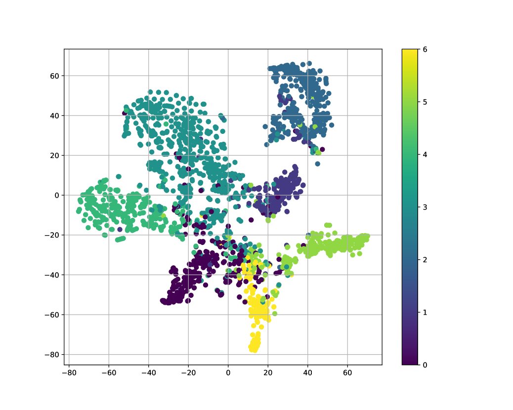
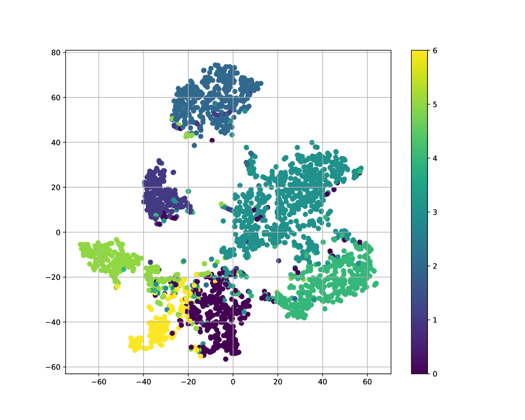
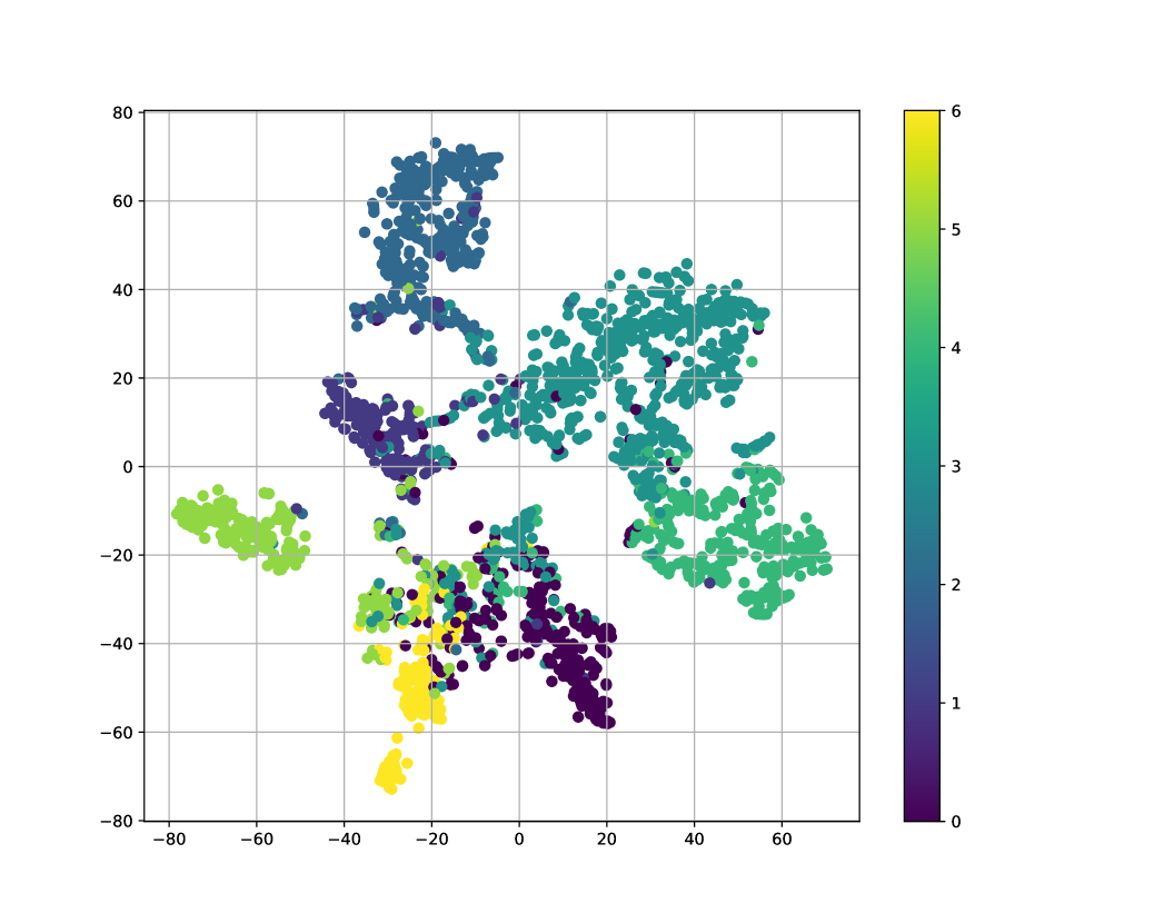
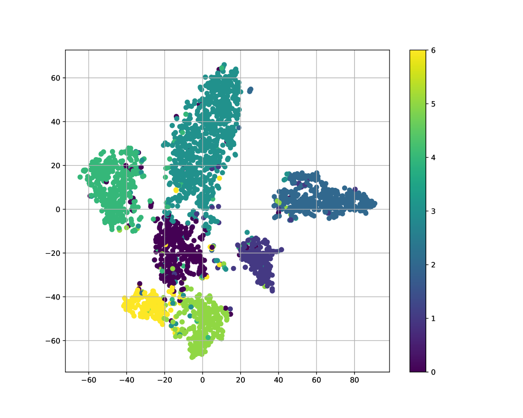
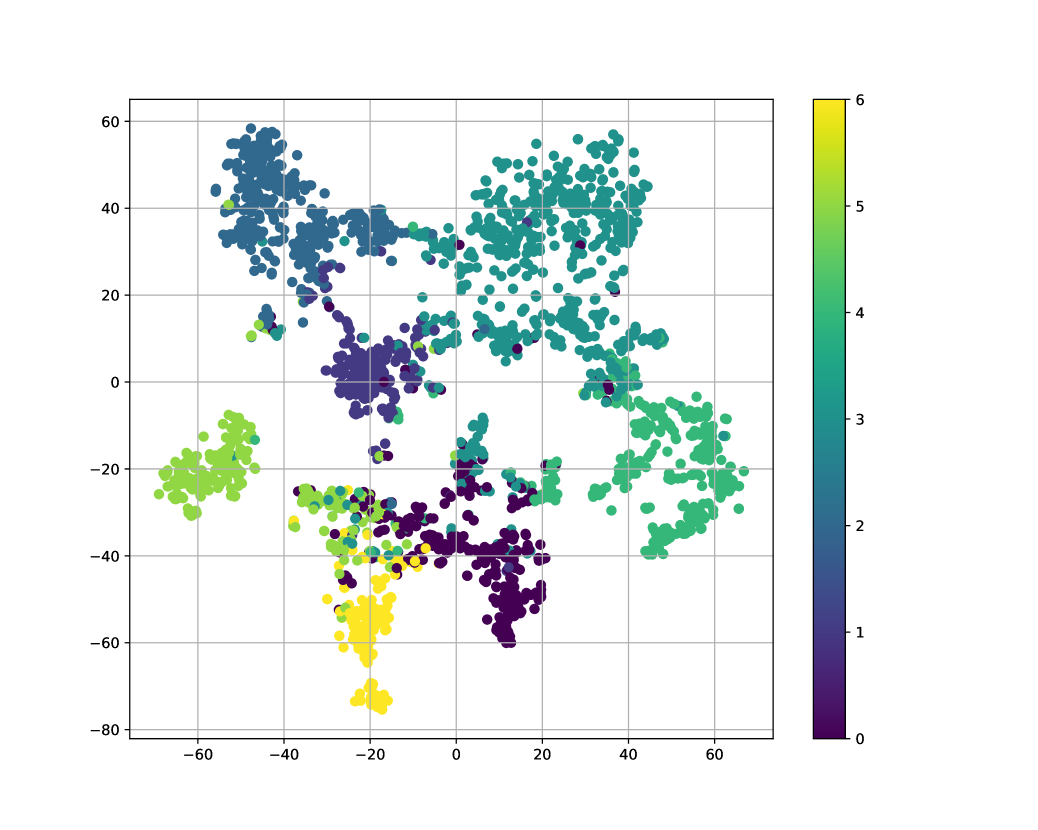
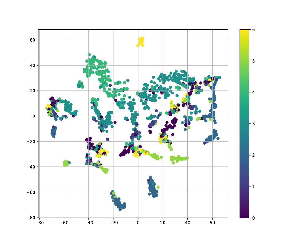
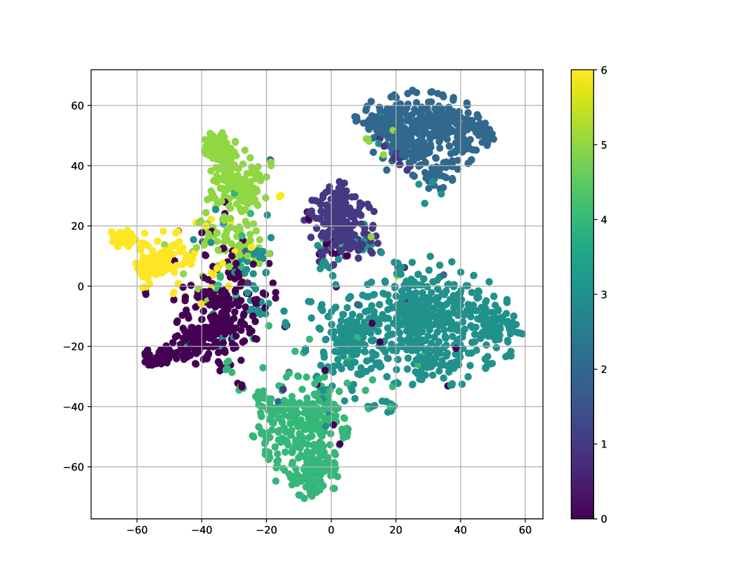
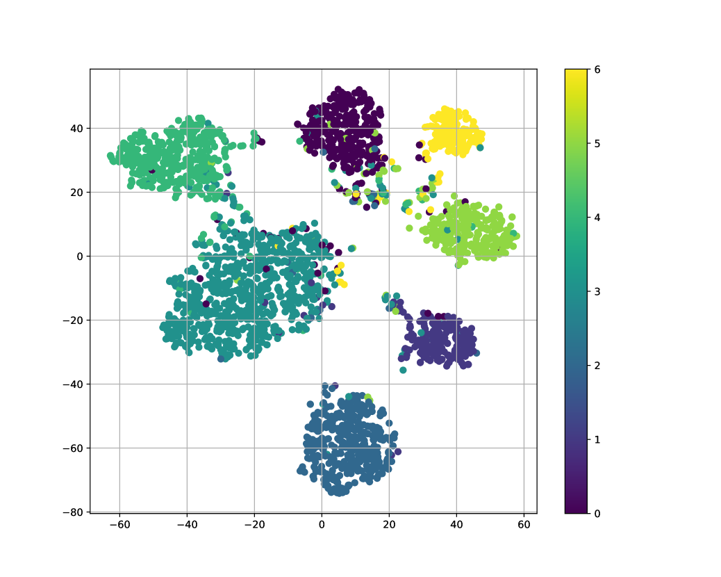
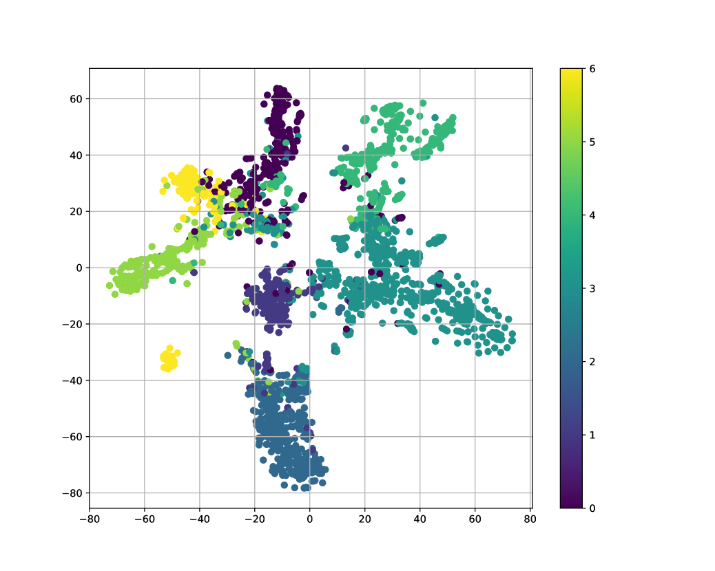
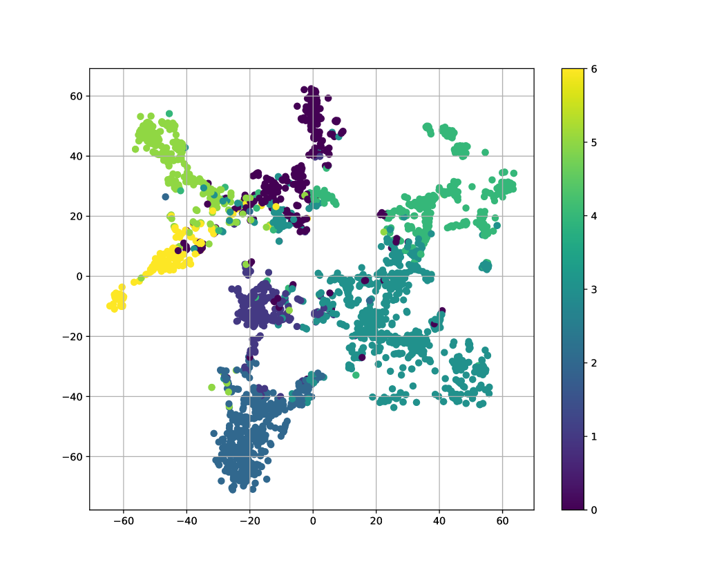
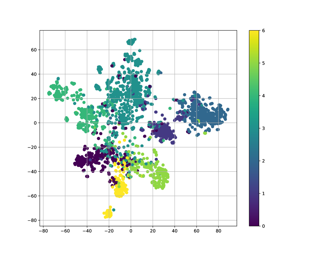
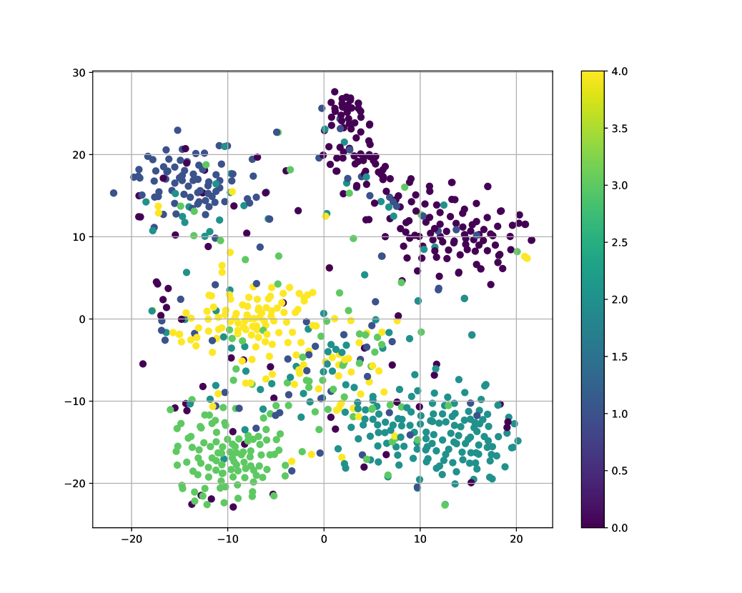
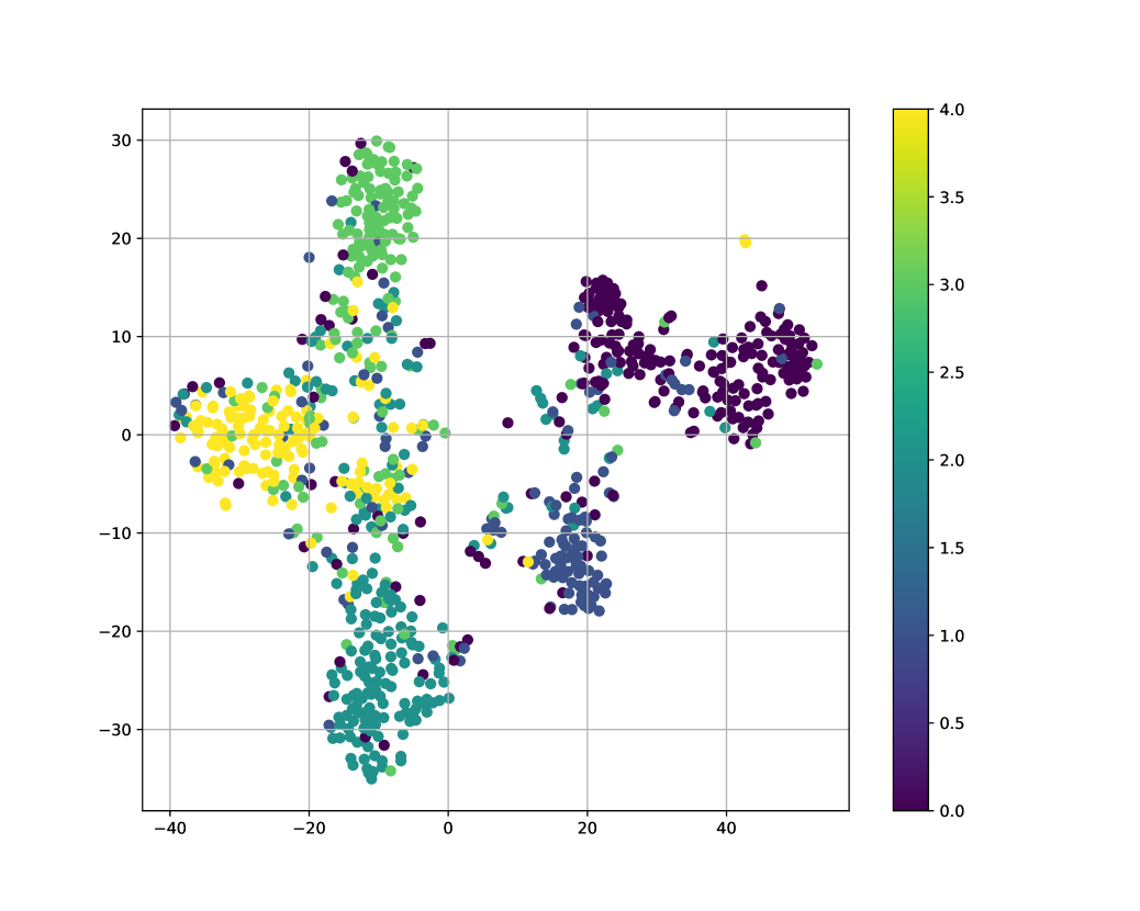
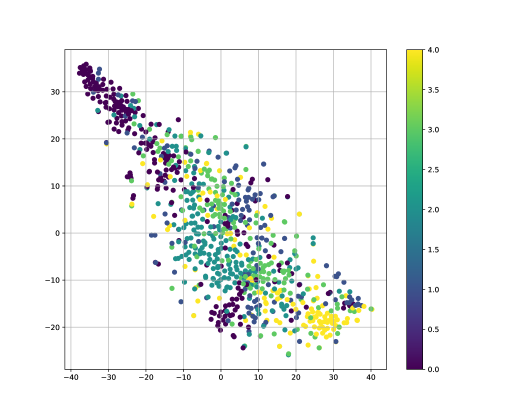
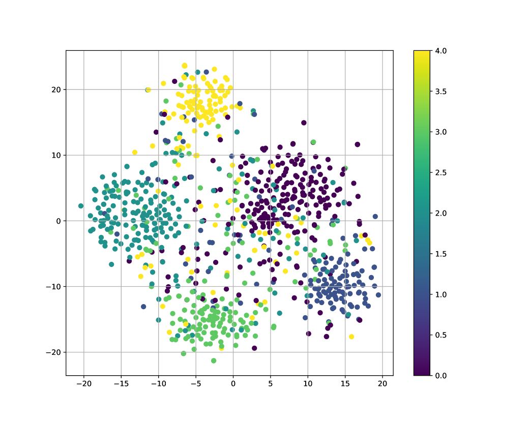
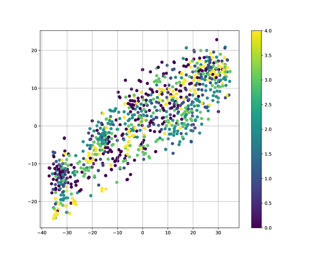
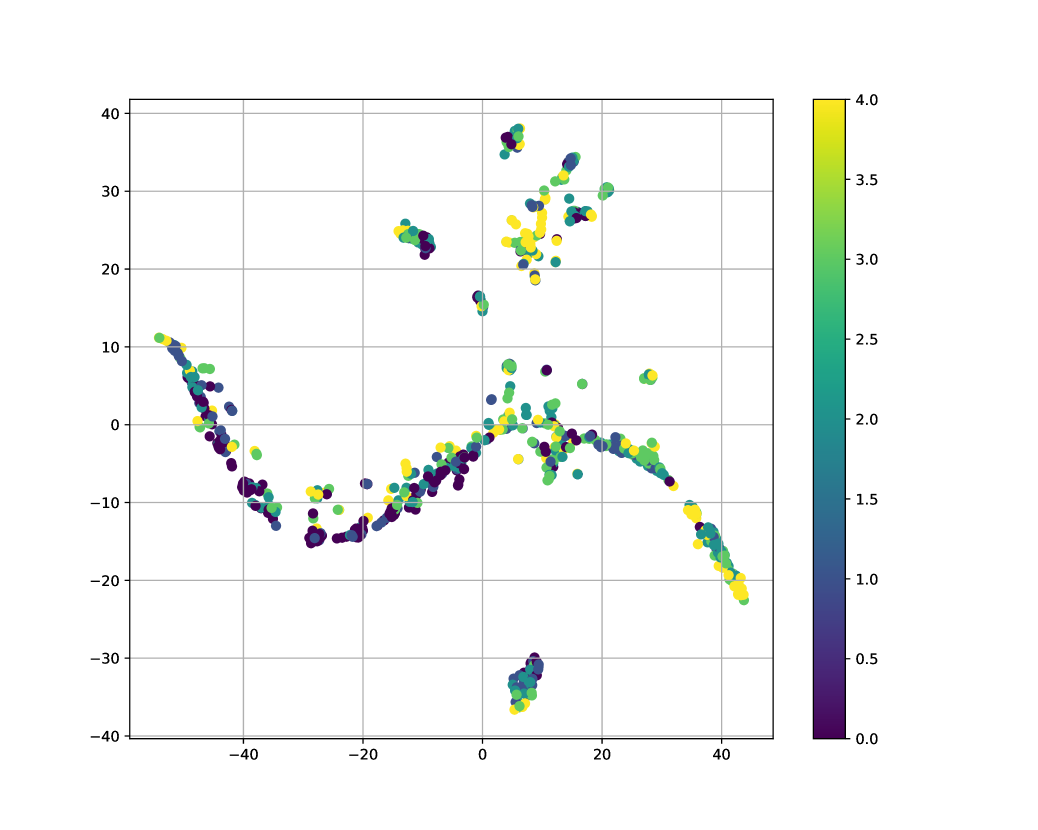
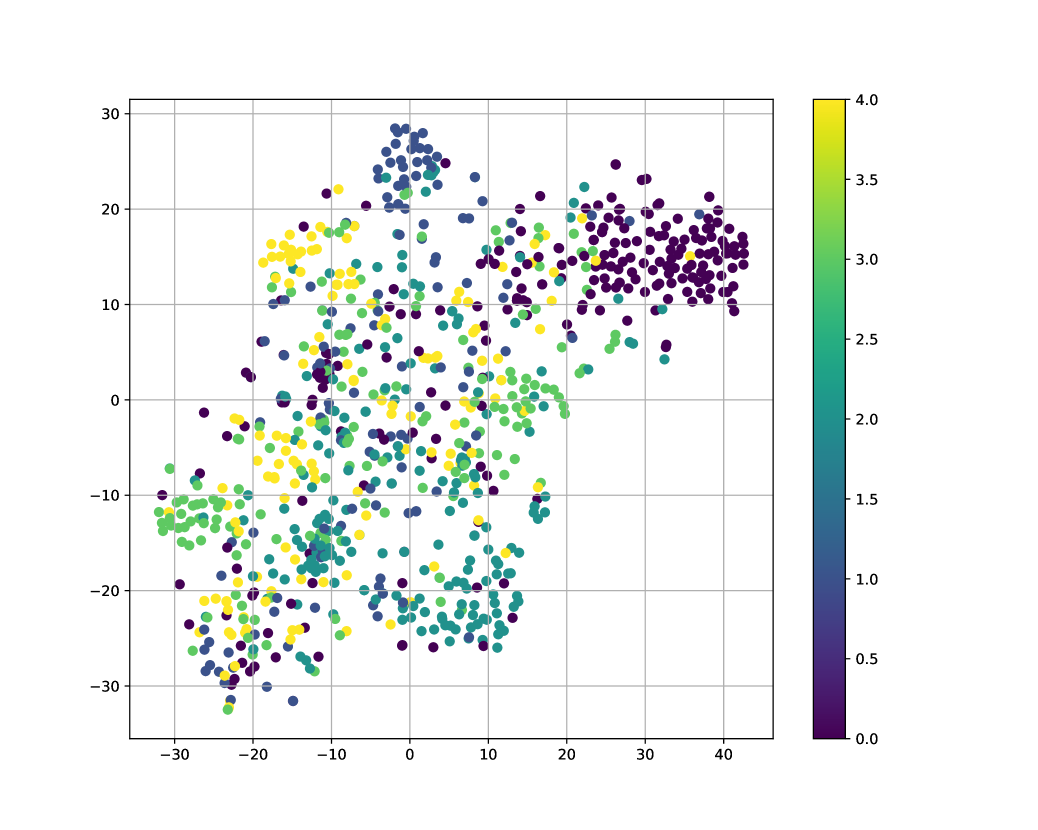
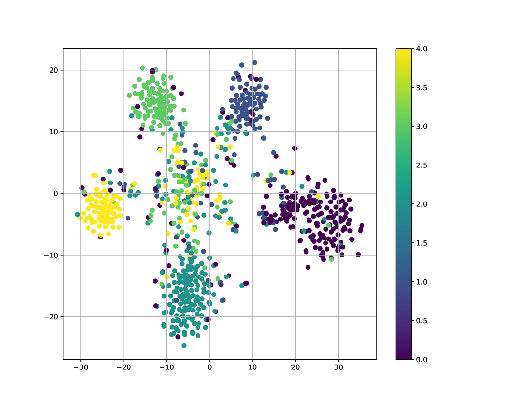
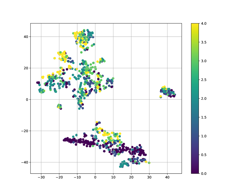
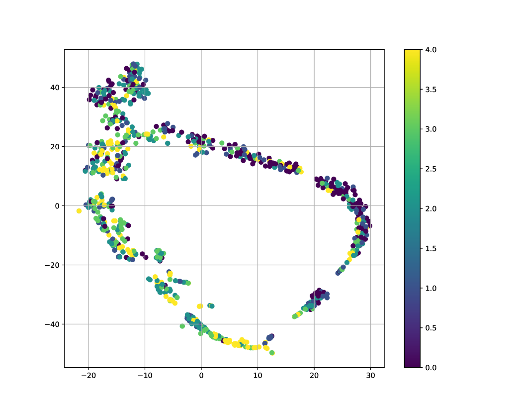
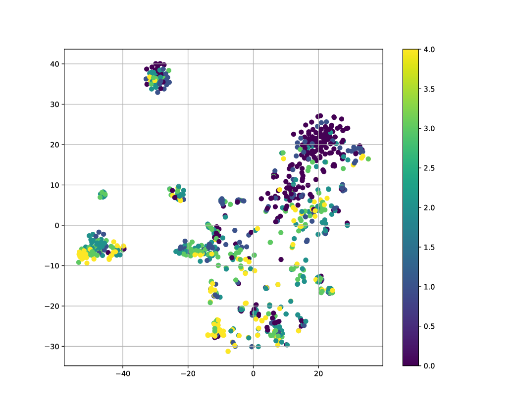
F.3 Effect of Propagation Hop
The number of propagation hops is an important hyperparameter affecting both spectral expressiveness and empirical efficiency. Hence, here we investigate the effect of the value of hops on model effectiveness. For analysis simplicity, filter bank models are omitted.
Figure 7 presents the pattern of model accuracy when changing the value of by discriminating fixed and variable filters on 4 classic homophilous graphs, while results for heterophilous graphs are in Figure 8. Overall, we showcase that our selection of in main experiments in reasonable for maintaining the performance of most models across various datasets. Below we respectively provide empirical analysis for each filter types.
For simple fixed filters, the efficacy gradually decreases when the hop number increases for both homophilous and heterophilous graphs, which corresponds to the over-smoothing issue. From the spectral perspective, this implies that the filtered signal overfits to the graph structure, and loses identity information embedded in the input signal. In contrast, fixed filters such as PPR and Gaussian can largely alleviate this issue by tuning the decaying factor.
The discussion on variable filters requires more detailed classification. Based on Appendix B, we learn that some variable filters are also homophily-centered, i.e., built on low-pass or band-reject bases in the frequency domain, such as Mono, Horner, and Bernstein, and Legendre. These filters exhibit a similar decreasing performance affected by . Other variable filters, especially those with orthogonal basis, are more stable when the propagation depth increases, demonstrating the flexibility of variable spectral filter design.
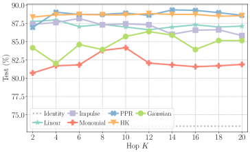

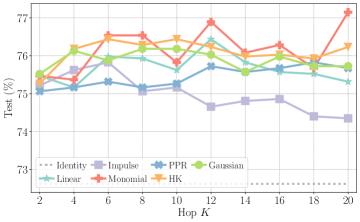
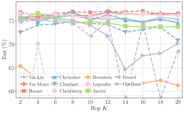
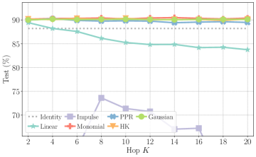
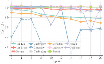
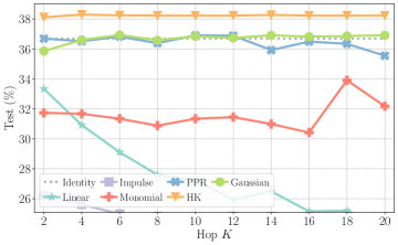
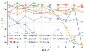

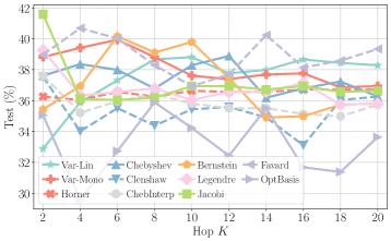
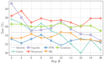
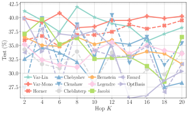
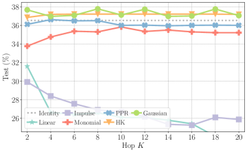
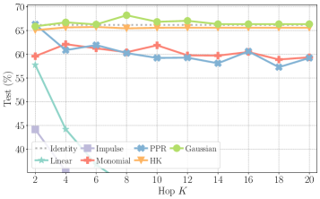
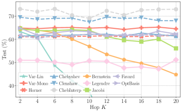
Appendix G Evaluation on Degree-wise Properties
Section 4.2 presents a preliminary study regarding the degree-specific performance of spectral models, including the high-level analysis across different models and datasets. In this section, we conduct more explorations on the impact factors of the phenomenon. It is revealed in previous studies that the existence of graph normalization affects the node-wise performance. For spectral GNNs, the normalization is often generalized to with tunable hyperparameter . Its value can be interpreted as the influence of in- and out-edge during graph signal processing. Specially, is the symmetric normalization with equal contributions from both directions.
We present experimental result of the accuracy gap between high- and low-degree nodes when varying in Figure 9. Only representative filters are shown for display clarity.
It can be observed from Figure 9 that, larger increases the difference value, i.e., improves the relative accuracy of high-degree nodes for both fixed and variable filters. Intuitively, it indicates that the in-bound information is useful for model inference on high-degree nodes. On graphs such as chameleon and actor where the utility of connection is hindered by heterophily, such a pattern is weaker and the performance gap becomes more unstable due to the complexity of graph conditions.
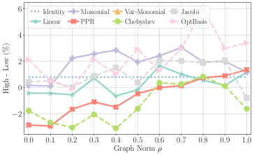
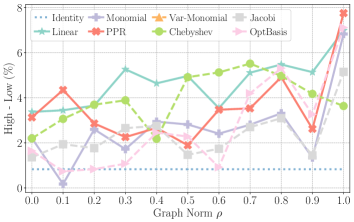
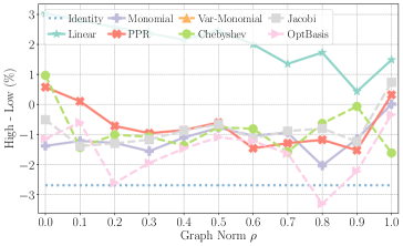
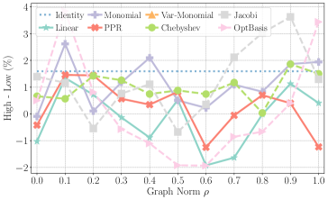
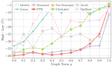
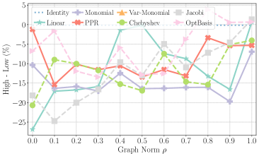
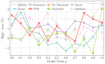
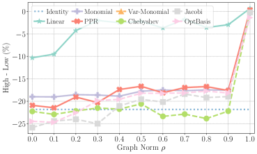
Appendix H Limitations and Future Plans
Our implementation framework is open-source and welcomes contributions. We also continuously maintain and upgrade the framework with more filters and relevant algorithms. A development roadmap with completion progress is available on the code repository for upcoming functionalities and features in the future.
Limitations.
We note the following limitations as for the current version of our framework. Firstly, more filters and algorithms can be analyzed and implemented. These include models in Section B.4 under a more general concept of spectral GNNs. Although they are limited in scalability, some designs in our framework are applicable to improve their efficiency. Secondly, the current implementation, especially the PyTorch-based propagation computation, can be further optimized for empirical scalability and efficiency. As algorithms introduced in Section B.4 are specialized for spectral models, they can be included for better runtime performance.
For our benchmark evaluation, we recognize that some operations proved effective in GNN tasks but without explicit spectral interpretations are not included, such as jumping knowledge [55], adjacency embedding [101, 21], and label smoothing [102]. Nonetheless, we note that these spatial designs are largely orthogonal to the spectral kernels, and can be integrated in parallel in practice to enhance performance.
Future Plans.
Despite the open questions raised in Section 5, we also append some future research directions towards better evaluation of GNN models. Our study underscores the importance of considering the efficacy-efficiency trade-off when evaluating spectral GNNs. It is possible to utilize synthetic graphs [13] to provide fine-grained controls on the factors affecting model performance for more dedicated assessment.
In addition, as our analysis illustrates the constancy of spectral kernels under different schemes, designing spectral GNNs can be regarded as combining different modules of filters, transformation, and parameterization schemes. Such process can be automated by Neural Architecture Search [103, 104] for a broader range of composition and more specific designs for different scenarios.
Broader Impact.
As our work primarily focuses on evaluating graph neural networks, we do not foresee it having a direct negative social impact.