ScaLES: Scalable Latent Exploration Score for Pre-Trained Generative Networks

Abstract

We develop Scalable Latent Exploration Score (ScaLES) to mitigate over-exploration in Latent Space Optimization (LSO), a popular method for solving black-box discrete optimization problems. LSO utilizes continuous optimization within the latent space of a Variational Autoencoder (VAE) and is known to be susceptible to over-exploration, which manifests in unrealistic solutions that reduce its practicality. ScaLES is an exact and theoretically motivated method leveraging the trained decoder’s approximation of the data distribution. ScaLES can be calculated with any existing decoder, e.g. from a VAE, without additional training, architectural changes, or access to the training data. Our evaluation across five LSO benchmark tasks and three VAE architectures demonstrates that ScaLES enhances the quality of the solutions while maintaining high objective values, leading to improvements over existing solutions. We believe that new avenues to LSO will be opened by ScaLES’ ability to identify out of distribution areas, differentiability, and computational tractability. Open source code for ScaLES is available at https://github.com/OmerRonen/scales.

1 Introduction

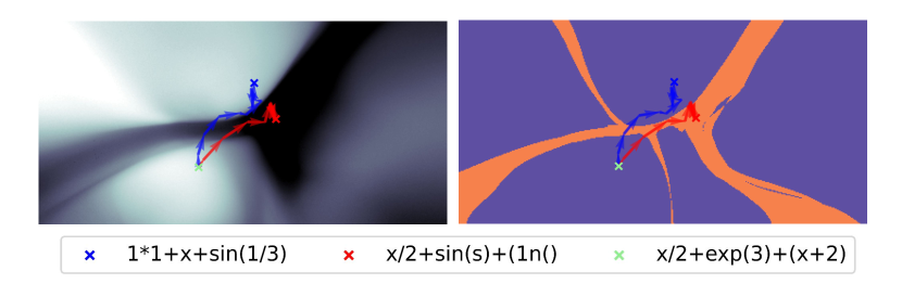
Figure 1: Incorporating ScaLES promotes valid solutions. We consider the task of approximating the expression 1/3 + x + sin(x * x), using LSO. Optimization trajectories with (blue) and without (red) ScaLES constraint in the latent space of a VAE are projected onto a two-dimensional subspace that contains the starting point and the end-points obtained after 10 gradient ascent steps. In the left panel, we show the ScaLES score for latent vectors on the two-dimensional subspace, with darker shades corresponding to lower ScaLES. In the right panel, we show the validity of the decoder outputs for each latent vector, with orange denoting invalid generations. High ScaLES values correlate with valid areas and incorporating ScaLES in LSO produce an expression that adheres to the grammatical rules of Example 1.1.

Optimization over discrete structured spaces is an important task with applications in scientific problems such as small molecule design and protein engineering. To improve the sample efficiency of discrete optimization algorithms, such as genetic algorithms, Latent Space Optimization (LSO) was recently developed (Gómez-Bombarelli et al., 2018). LSO transfers the optimization problem to the domain of the latent space of a VAE, which can be efficiently explored using continuous optimization techniques. However, ensuring that LSO solutions respect the structure of the original space remains a challenge. To illustrate this issue, we first provide some examples of such structures.

Example 1.1 (Arithmetic expressions).

An expression built up using numbers, arithmetic operators and parentheses is called an arithmetic expression. However, not every sequence of the above elements correspond to a valid expression. For instance the expression "sin(x) + x" is a valid expression while "sin(xxx" is not.

Example 1.2 (Simplified molecular-input line-entry system (SMILES)).

SMILES provides a syntax to describe molecules using short ASCII strings. Atoms are represented by letters (e.g. water:"O", methane:"C", …), bonds are represented by symbols (e.g. triple: "#", double: "=", … ), branches are represented in parentheses and cyclic structures are represented by inserting numbers at the beginning and the end. Like the arithmetic expressions case, not every combination of the elements described above corresponds to a valid molecule. For example while "C1CCCCC1" is valid, both "C1CCCCC2" and "C1CCCCC)" are not.

Example 1.3 (Quality filters for molecules).

Chemists often seek molecules that not only optimize desired chemical properties but are also stable and easy to synthesize. This has led to the development of rules such as Lipinski’s Rule of Five (RO5, Lipinski et al. (1997)), which helps determine if the bioavailability (i.e., the proportion of a drug or other substance that enters the circulation when introduced into the body) of a given compound meets a certain threshold. For example, RO5 suggests that poor absorption is more likely when the octanol-water partition coefficient (logP) exceeds 5. Similarly, the Pan Assay Interference Compounds (PAINS, Baell and Holloway (2010)) filter helps in identifying false positives in assay screenings. Recently, the rd_filters (Walters, 2019) package has curated many such rules and is considered a "high precision, low recall surrogate measure" (Brown et al., 2019). Following Notin et al. (2021) we consider a sample valid if it passes the rd_filters quality filters

Numerous directions have been explored to overcome the challenge of providing valid solutions including specialized VAE architectures (Kusner et al., 2017; Jin et al., 2018) or training procedures (Tripp et al., 2020) and robust representations for discrete data (Krenn et al., 2020). Additionally, constrained objectives can be formulated under the assumption that one has access to a function which quantifies the validity of any point in the latent space (Griffiths and Hernández-Lobato, 2020). However, in many realistic scenarios, such as Example 1.3, these solutions may not be directly applicable, as the structure of the sequence space may not be sufficiently well understood. To address this, Notin et al. (2021) proposed using an uncertainty estimator for the variational approximation to a posterior distribution over the VAE parameters, encouraging LSO to respect the sequence space structure. Although this approach proved effective, the non-differentiable nature of the uncertainty score required its integration into LSO through heuristic approaches. Additionally, the computation of the uncertainty score is not exact (i.e., it relies on variational approximation and monte carlo sampling) and requires significant amount of time to compute. Therefore, there is a need for robust, general-purpose methods that work across different VAEs and sequence space structures, and can be easily integrated into existing LSO pipelines.

Motivated by this goal, we develop ScaLES, a score that can be used as a constraint in LSO optimization to increase the number of solutions that respect a given structure. The distinctive characteristics of ScaLES are differentiability and scalability that allow its easy integration into existing LSO pipelines. Specifically our contributions include:

• We derive ScaLES, a score with higher values in areas closer to the training data. We show that ScaLES can efficiently identify areas in the latent space that respect the sequence space structure.

• We develop a numerically stable optimization procedure to incorporate ScaLES as a constraint in LSO.

• We evaluate ScaLES-constrained LSO across three VAEs and five benchmark tasks, demonstrating its robustness in promoting valid solutions as well as its benefits in achieving high objective values.

Open source code for ScaLES is available at https://github.com/OmerRonen/scales.

2 Background: Latent Space Optimization

LSO is a method for solving black box optimization problems in discrete and structured spaces, such as the space of valid arithmetic expressions. Formally, let $\mathcal{V}\subset\mathbb{R}^{\textup{L}\times\textup{D}}$ be a discrete and structured space, represented as a sequence of L one-hot vectors of dimension D. We represent sequences of length L of categorical variables with D categories. L is set as the maximum sequence length that we are optimizing for, and one of the D categories is used as an "empty" category. For instance, in the case of valid arithmetic expressions, $\mathcal{V}$ would be the set of all sequences that define such expressions. Let $\mathcal{M}:\mathcal{V}\rightarrow\mathbb{R}$ be the objective function. LSO aims to solve,

$$\arg\max_{x\in\mathcal{V}}\mathcal{M}(x).$$ (1)

In this setting, we assume that evaluations of the objective function ($\mathcal{M}$) are expensive to conduct. For example, the objective may be the binding affinity for a given protein, measured through a wet lab experiment. A popular approach to solve Equation 1 is Bayesian Optimization (BO), which utilizes first order optimization of a surrogate model for $\mathcal{M}$. However, since the space is discrete, first order optimization cannot be directly applied.

In an attempt to make BO applicable for solving Equation 1, Gómez-Bombarelli et al. (2018) proposed to transfer the optimization problem into that over a domain of the latent space of a deep generative model and subsequently perform BO in this space. The main idea is to (1) learn a continuous representation of the discrete objects (e.g., using a VAE) and (2) perform BO in the latent space while decoding the solution at each step. Formally, given a pre-trained encoder ($\mathbf{E}_{\theta}$) and decoder ($\mathbf{G}_{\theta}$) the initial labelled dataset $\mathcal{D}=\{\bm{x}_{i},y_{i}\}_{i=1}^{n}$ is first encoded into the latent space $\mathcal{D}^{\bm{z}}=\{\bm{z}_{i}=\mathbf{E}_{\theta}(\bm{x}_{i}),y_{i}\}_{i=1}^{n}$. Using the encoded dataset, an iterative BO procedure is conducted, which we describe in Algorithm 1. Most commonly, a Gaussian process is used as the surrogate model for $\mathcal{M}$ , and the acquisition function is the expected improvement, defined as (Frazier, 2018)

$$\mathbb{E}\max(\hat{f}(x)-f^{\star},0),$$ (2)

where $f^{\star}$ is the best observed objective value and the expectation is with respect to the posterior of $\hat{f}$.

Algorithm 1 Latent Space Optimization

for $t=1$ to $T$ do

1. Fit a surrogate model $\hat{f}$ to the encoded dataset, $\mathcal{D}^{\bm{z}}$

2. Generate a new batch of query point by optimizing a chosen acquisition function ($\mathcal{A}$)

   $$\bm{z}^{(\text{new})}=\arg\max_{\bm{z}}\mathcal{A}(\hat{f}(\bm{z}))$$ (3)

3. Decode $\bm{x}^{(\text{new})}=\mathbf{G}_{\theta}(\bm{z}^{(\text{new})})$, evaluate the corresponding true objective values ($y^{\text{new}}=\mathcal{M}(\bm{x}^{(\text{new})})$) and update $\mathcal{D}^{\bm{z}}$ with ($\bm{z}^{(\text{new})},y^{\text{new}}$).

Over-exploration in LSO

Multiple studies (Notin et al., 2021; Kusner et al., 2017) have found that unconstrained LSO often produces solutions that ignore the above mentioned structures. For example, in searching arithmetic expressions, invalid equations like "$ssin(xxx$" are common. Similarly, many solutions in molecule searches fail the rd_filters filters, making them of limited practical use.

To mitigate over-exploration, we propose adding a penalty to Equation 3. The penalty uses a new score, giving higher values over the latent space valid set, defined as:

Definition 2.1 (Latent space valid set).

Let $\mathbf{G}_{\theta}:\mathcal{Z}\rightarrow\mathbb{R}^{\textup{L}\times\textup{D}}$ be a decoder network, and let $\mathcal{V}\subset\mathbb{R}^{\textup{L}\times\textup{D}}$ be the set of valid sequences, the latent space valid set is defined as

$$\{\bm{z};\mathbf{G}_{\theta}(\bm{z})\in\mathcal{V}\}.$$ (4)

The derivation of our score leverages the Continuous Piecewise Affine (CPA) representation of neural networks, which we briefly review below.

Deep generative networks as CPA

Following Humayun et al. (2022, 2021); Balestriero and Baraniuk (2018), we consider the representation of Deep Generative Networks (DGNs) as Continues Piecewise Affine (CPA) Splines operators. Let $f_{\theta}$ be any neural network with affine layers and piecewise affine activations then it holds that

$$f_{\theta}(\bm{z})=\sum_{\omega\in\Omega}\left(\bm{A}_{\omega}\bm{z}+\bm{b}_{\omega}\right)1_{\{\bm{z}\in\omega\}},$$ (5)

where $\Omega$ is the input space partition induced by $f_{\theta}$, $\omega$ is a particular region and the parameters $\bm{A}_{\omega}$ and $\bm{b}_{\omega}$ defines the affine transformation depending on $\omega$.

In the cases where $f_{\theta}$ is not comprised of only piecewise affine layers and activations, we leverage the result from Daubechies et al. (2022) to assert that Equation 5 is either an exact representation of $f_{\theta}$ or is a sufficiently accurate approximation of $f_{\theta}$ for our practical purposes Humayun et al. (2022).

3 A Scalable Latent Exploration Score to Reduce Over-Exploration in LSO

In this section, we introduce Scalable Latent Exploration Score (ScaLES), our new score to reduce over-exploration in LSO. First, we motivate our score in Section 3.1. Next, we formally derive ScaLES in Section 3.2. In Section 3.3, we provide evidence that ScaLES gives higher values in the latent space valid set. The use of ScaLES to regularize or contrain LSO is left for Section 4.

3.1 Motivation

Our goal is to develop a meaningful constraint for optimizing the acquisition function. We seek a constraint that is a continuous function of $\bm{z}$, achieving higher values in valid regions of the latent space (Definition 2.1). Assuming most of VAE training data is valid, the score should be higher in regions near training data points. To achieve this, we treat the latent space of the VAE as a probability space, i.e. $\bm{z}\sim p_{\bm{z}}$, for some prior distribution $p$ (most commonly standard Gaussian). The prior should reflect our best guess for the distribution of the observed data in the latent space. Solutions are mapped back to the sequences by the decoder through a deterministic transformation of the latent solution vectors. Therefore, any distribution on the latent space defines a distribution over the space of sequences. Our score uses the density function of the push-forward measure of $\bm{x}=\mathbf{G}_{\theta}(\bm{z})$, which we call the sequence density. Our score considers only the decoder network, not the encoder, and can potentially be applied to other generative models like GANs or diffusion models.

Why use the sequence density function?

We argue that, for a well-trained decoder network, the density should be higher in areas of the sequence space close to the training data. To see why, consider a decoding model $\mathbf{G}_{\theta}$ trained on a dataset $\{(\bm{z}_{i},\bm{x}_{i})\}_{i=1}^{n}$. The average loss at $\bm{z}$ is

$$\ell(\mathbf{G}_{\theta}(\bm{z}))=\mathbb{E}_{\bm{x}|\mathbf{E}_{\theta}(\bm{x})=\bm{z}}L(\mathbf{G}_{\theta}(\bm{z}),\bm{x}).$$ (6)

As the training process is designed to minimize the population loss: $\mathbb{E}\ell(\mathbf{G}_{\theta}(\bm{z}))$, if successful, we hypothesize that the distribution of $\mathbf{G}_{\theta}(\bm{z})$ puts higher weight in the areas where $\ell(\mathbf{G}_{\theta}(\bm{z}))$ is low. Since we expect most of the training data to be valid and to achieve low expected loss, the sequence density should put higher weight on the latent space valid set. Section 3.3 provides an empirical validation for this hypothesis, for Examples 1.1, 1.2 and 1.3. We highlight that this relationship between the valid set and the sequence density depends on how well the decoder fits the data.

3.2 Derivation of ScaLES

Analytical formula for ScaLES

DGNs for discrete sequences typically output a matrix of logits, transformed into normalized scores by the softmax function:

$$\mathbf{G}_{\theta}(\bm{z})=\text{Softmax}(\mathbf{L}_{\theta}(\bm{z})).$$ (7)

$\mathbf{L}_{\theta}(\bm{z})$ is a $\textup{D}\times\textup{L}$ logits matrix and Softmax is the softmax operation applied to every column of $\mathbf{L}_{\theta}(\bm{z})$. Our derivation requires $\mathbf{G}_{\theta}$ to be bijective, and we therefore extend the output of the function to include the normalizing constant for each column. With this form, we can now derive the sequence density function.

Theorem 3.1 (DGN sequence density).

Let

$$\mathbf{G}_{\theta}(\bm{z}) =\left(\bm{p}^{(1)}_{\bm{z}},c^{(1)}_{\bm{z}},\dots,\bm{p}^{(L)}_{\bm{z}},c^{(L)}_{\bm{z}}\right)$$ (8)

$$=\bm{x}_{\bm{z}}$$ (9)

where $\bm{p}^{(i)}_{\bm{z}}=\text{Softmax}(\mathbf{L}_{\theta}(\bm{z}))_{.i}$ and $c^{(i)}_{\bm{z}}=\sum_{j=1}^{D}e^{\mathbf{L}_{\theta}(\bm{z})_{ji}}$. Assume that $\mathbf{L}_{\theta}$ is bijective and can be expressed as a CPA (Equation 5), and that $\bm{z}\sim p_{\bm{z}}$, then the density function of $\mathbf{G}_{\theta}(\bm{z})$ is given by:

$$f_{\bm{z}}(\bm{z})\sqrt{\det\left(\sum_{i=1}^{\textup{L}}(\bm{A}^{\dagger}_{i})^{T}(\bm{B}_{i})^{T}\bm{B}_{i}\bm{A}^{\dagger}_{i}\right)}$$ (10)

for

$$\bm{B}_{i} =\left(\text{diag}\left(\frac{1}{(\bm{p}^{(i)}_{\bm{z}})_{1}},\dots,\frac{1}{(\bm{p}^{(i)}_{\bm{z}})_{\textup{D}}}\right),\bm{1}\frac{1}{c^{(i)}_{\bm{z}}}\right)^{T}$$ (11)

$$\bm{A}^{\dagger}_{i} =\left(\bm{A}^{(1)}_{\omega},\dots,\bm{A}^{(L)}_{\omega}\right)^{\dagger}_{(i\cdot\textup{D}):(i+1\cdot\textup{D}).},$$ (12)

where $\left(\bm{A}^{(1)}_{\omega},\dots,\bm{A}^{(L)}_{\omega}\right)^{\dagger}$ is the Moore–Penrose inverse of $\left(\bm{A}^{(1)}_{\omega},\dots,\bm{A}^{(L)}_{\omega}\right)$.

We provide the proof in Appendix A. In practice, we define ScaLES to be the log sequence density with an additional weight parameter $\rho$,

$$\mathcal{S}_{\rho}(\bm{z}) =\log(f_{\bm{z}}(\bm{z}))+\rho\log\left(\sqrt{\det\left(\sum_{i=1}^{\textup{L}}(\bm{A}^{\dagger}_{i})^{T}(\bm{B}_{i})^{T}\bm{B}_{i}\bm{A}^{\dagger}_{i}\right)}\right).$$ (13)

The parameter $\rho$ should be lower in the cases where the prior we put on the latent space is accurate, and can be calibrated using a small labelled dataset.

Remark 3.2.

In our experiments we do not verify that the conditions of Theorem 3.1 hold, rather we naively calculate $\mathcal{S}$ as defined in Equation 13.

3.3 Validating the relationship between ScaLES and valid generation

To assess ScaLES’s ability to identify validity as defined in Examples 1.1, 1.2 and 1.3, we sample data points in the latent space for each dataset using the VAEs studied in Section 4. Specifically, we sample 500 data points, from four distributions: train, test, prior ($\mathcal{N}(\bm{0},\bm{I})$), and out-of-distribution ($\mathcal{N}(\bm{0},\bm{I}\cdot 20)$). We decode each data point and determine if the decoded sequence is valid.

We treat identifying if a point in the latent space decodes into a valid sequence as a classification problem. We measure performance using the AUROC metric. For ScaLES, we tune $\rho$ to achieve high AUROC. Besides ScaLES and the Bayesian uncertainty score, we add two baseline scores for comparison. The first is the density of a standard Gaussian (Prior), a naive OOD score not based on the decoder network. This helps us understand the log determinant term of ScaLES. The second is the polarity score (Humayun et al., 2022), showing the gains due to accounting for the softmax non-linearity Theorem 3.1. The results are shown in Table 1. ScaLES improves on the polarity and prior scores in all cases. While the uncertainty score does better on the SMILES and expressions datasets, ScaLES is much better in the SELFIES dataset, showing its robustness. Unlike the expressions and SMILES datasets, many points in the SELFIES training set fail to pass quality filters. However, an analysis using the first 20k training points from Maus et al. (2022) shows lower ELBO and reconstruction losses for molecules that pass the filters (ELBO: 0.2 vs. 0.3, reconstruction: 0.163 vs. 0.26). This supports our belief that ScaLES values are higher where the decoder fits the data well.

Table 1: AUROC for identifying valid data points. ScaLES outperforms both the polarity score and Prior across all three datasets and significantly improves upon UC for the SELFIES dataset.

	ScaLES ($\rho$)	UC	Prior	Polarity
Expressions	0.94 (1)	0.96	0.64	0.92
SMILES	0.88 (.01)	0.96	0.52	0.85
SELFIES	0.78 (.003)	0.39	0.76	0.76

4 ScaLES-constrained LSO

Our investigation in Section 3.3 shows that ScaLES is a robust score that obtains higher values in the latent space valid set (Definition 2.1). Furthermore, ScaLES is differentiable which means it can easily be used to constrain any optimization problem.

Specifically, we propose adding an explicit constraint to Equation 3, encouraging the solution to achieve a high ScaLES value. We modify Algorithm 1 by penalizing step (2) as follows:

$$\bm{z}^{\text{new}}=\arg\max_{\bm{z}}\mathcal{A}(\hat{f}(\bm{z}))+{\color[rgb]{0,0,1}\lambda\mathcal{S}(\bm{z})}.$$ (14)

Computing ScaLES

$\mathcal{S}(\bm{z})$ is a function of the prior of $\bm{z}$ and the matrices $\bm{B}_{i}$ and $\bm{A}_{i}^{\dagger}$.
The prior of $\bm{z}$ is typically a Gaussian distribution and can be easily computed. The matrices $\bm{B}_{i}$ are function of the logits and can be calculated using a single forward run of $\mathbf{G}_{\theta}$. The matrices $\bm{A}^{\dagger}_{i}$ are a function of $\bm{A}_{\omega}$, which is equal to the derivative of $\mathbf{L}_{\theta}$ at $\bm{z}$. Therefore $\bm{A}_{\omega}$ can be obtained using automatic differentiation, which can be efficiently done using PyTorch (Paszke et al., 2017).
$\mathcal{S}(\bm{z})$ is computed by performing all of the above calculations in parallel using a single forward call to the $\mathbf{G}_{\theta}$ network. In addition, we need to compute the pseudo-inverse of $\bm{A}_{\omega}$, which has a computational complexity of $\mathcal{O}(\textup{L}^{2}\textup{D}+\textup{D}^{3})$. To accelerate ScaLES computation, we approximate $\bm{A}_{\omega}$ using discrete derivatives with $\epsilon=1\times 10^{-4}$. In addition, for the SMILES and SELFIES datasets, we limit the output sequence to the first 30 and 60 elements, respectively. Appendix C provides a detailed description of the wall clock times.

4.1 Experimental setup

LSO setup

Throughout our experiments, following Notin et al. (2021), we consider the batched BO setting in which we generate a batch of 5 query points at each iteration of Algorithm 1. A Gaussian process is used as our surrogate model for the true objective $\mathcal{M}$, where in the case of SELFIES-VAE (Maus et al., 2022), we deploy a deep-kernel since the latent space is high-dimensional (256), with the same specification as in Maus et al. (2022). We use the log expected improvement (Ament et al., 2024) as our acquisition function, to avoid vanishing gradients, which we sequentially maximize.

LSO benchmarks

We study the LSO tasks previously studied in Notin et al. (2021); Maus et al. (2022). Section B.1 provides the specifications of the LSO problems studied in this section.

Acquisition function optimization

For ease of implementation, we focus on a simple optimization procedure in which the acquisition function (Equation 3) is optimized with 10 steps of normalized gradient ascent, to ensure numeric stability. To make sure this procedure is not overly simplistic, we also compare with the default optimization method implemented in the BoTorch (Balandat et al., 2020) package (optimize_acqf function, which implements the L-BFGS quasi-newton algorithm Liu and Nocedal (1989)).

Numeric stability

In our experiments we find that the norm of the derivative of the constraint (i.e., $\mathcal{S}(\bm{z})$) if typically much larger than the norm of the derivative of the acquisition function. As a result, using the gradient ascent update rule $\bm{z}^{(i+1)}=\partial\mathcal{A}(\hat{f}(\bm{z}^{(i)}))+\lambda\partial\mathcal{S}(\bm{z}^{(i)})$ results in a numerically unstable optimization procedure. To overcome this challenge, we propose the update rule:

$$\bm{z}^{(i+1)}=\frac{\partial\mathcal{A}(\hat{f}(\bm{z}^{(i)}))}{\|\partial\mathcal{A}(\hat{f}(\bm{z}^{(i)}))\|_{2}}+\lambda\frac{\partial\mathcal{S}_{\rho}(\bm{z}^{(i)})}{\|\partial\mathcal{S}_{\rho}(\bm{z}^{(i)})\|_{2}}.$$ (15)

We find that selecting $\lambda=0.5$ improves over vanilla methods and is recommended as a default value, and we leave data-driven, adaptive selection of $\lambda$ for future work.

Methods

We consider the following optimization methods, all use the optimization technique above except L-BFGS:

• ScaLES - ScaLES-constrained LSO, we use $\lambda=0.2,0.5,0.8$ to ensure the constraint does not dominate the objective.

• LSO (GA) - gradient ascent with no regularization.

• Prior - the prior distribution over the latent space is a standard Gaussian. We use the prior density as a constraint similar to Equation 14. We consider $\lambda=0.2,0.5,0.8$.

• UC - the Uncertainty Constrained gradient ascent method by Notin et al. (2021). The Bayesian uncertainty score serves as an early stopping criterion: if the updated point’s score exceeds a set threshold, we reject the update. The threshold is based on the 75th, 95th, and 100th percentiles of the training data, as in Notin et al. (2021). To avoid long run times, we sample 10 times from the model parameters and the importance distribution. Indeed, with this choice our results are qualitatively similar to Notin et al. (2021).

• LSO (L-BFGS) - L-BFGS in a hyper-cubic search region, the L-BFGS algorithm returns solutions within a hypercube centered at zero. We normalize latent space vectors to between zero and one, considering facet lengths of 1, 5, and 10. The first explores within the data manifold, while the last two also explore outside it.

Hyperparameters

We calibrate the step size such that our gradient ascent procedure successfully and consistently improve the values of the acquisition function, across different initializations. Indeed, our final optimization results match those of earlier studies (Kusner et al., 2017; Notin et al., 2021). We adopt the values of $\rho$ used in Section 3.

4.2 Results

4.2.1 Expressions and logP

We start by evaluating ScaLES on two of the most extensively studied LSO tasks: approximating arithmetic expressions and optimizing the penalized water-octanol partition coefficient (logP) over the SMILES representation of molecules.

Arithmetic expression approximation

The arithmetic expressions we consider are functions of a single variable (e.g., $\sin(x)$, $1+x*x$). Our goal is to find an expression approximating 1/3 + x + sin(x * x) Kusner et al. (2017). We train a Character VAE (CVAE) using the same procedure as Notin et al. (2021). We start BO with 500 randomly selected data points from the training set, encoded into the latent space with their objective values. We perform 100 BO steps with a learning rate of 0.5, using the validity notion from Example 1.1.

logP over molecules

The Octanol-water partition coefficient is a measure of how hydrophilic or hydrophobic a chemical substance is. It is calculated using the prediction model developed by Wildman and Crippen (1999). We train a Character VAE (CVAE) following the same training procedure as Notin et al. (2021). We initialize the BO with 500 data points from the training set, selected at random and encoded into the latent space, along with their objective values. We perform 100 steps of BO and use a learning rate of 0.01. Adopting the notion of validity of Example 1.2.

Optimization results

Figure 2 shows the cumulative best solution (i.e., highest $\mathcal{M}$ value) and the average of the top 10 solutions across BO steps for expressions and molecules. Table 2 displays the relationship between regularization strength and the percentage of valid solutions generated during BO, the value $\lambda=2$ is added as it increases the percentage of valid solutions. Increasing regularization strength leads to more valid solutions for both tasks. While UC produces the most valid solutions, compared to ScaLES, using ScaLES as an early stopping method (ScaLES (ES)) shows that this difference is mainly due to the optimization process. For the expressions task, the best-performing ScaLES method has an average top 10 value of -0.49 (0.02) compared to -0.53 (0.01) for UC. For the logP task, ScaLES achieves an average top 10 value of 2.6 (0.09) compared to 2.53 (0.05) for UC. We provide the full optimization results in Sections B.4 and B.3.

Table 2: Percentage of valid solutions generated through the BO procedure for logP and expressions tasks. Throughout the entire optimization, 500 solutions are produced for each task. Regularizing using ScaLES significantly increases the proportion of valid solutions. Although UC yields a higher number of valid solutions than ScaLES, employing ScaLES as an early stopping (ES) method indicates that most of the improvement arises from the ES algorithm itself, rather than the quality of the score.

Method	Reg.	Expressions	logP
LSO (GA)		70% (1)	18% (0.5)
ScaLES	$\lambda$ = 0.2	87% (1)	23% (1)
	$\lambda$ = 0.5	92% (0.5)	28% (1)
	$\lambda$ = 0.8	93% (0.5)	35% (1)
	$\lambda$ = 2	95% (0.2)	47% (1)
UC	75th quantile	99.5% (0.1)	70% (1)
	95th quantile	98% (0.2)	70% (1)
	100th quantile	76% (0.1)	70% (1)
ScaLES (ES)	25th quantile	92% (0.3)	37% (1)
	50th quantile	94% (0.2)	53% (1)
	75th quantile	95% (0.2)	62% (1)

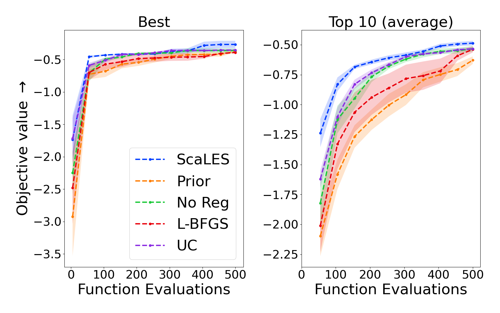
(a) Arithmetic expression approximation.

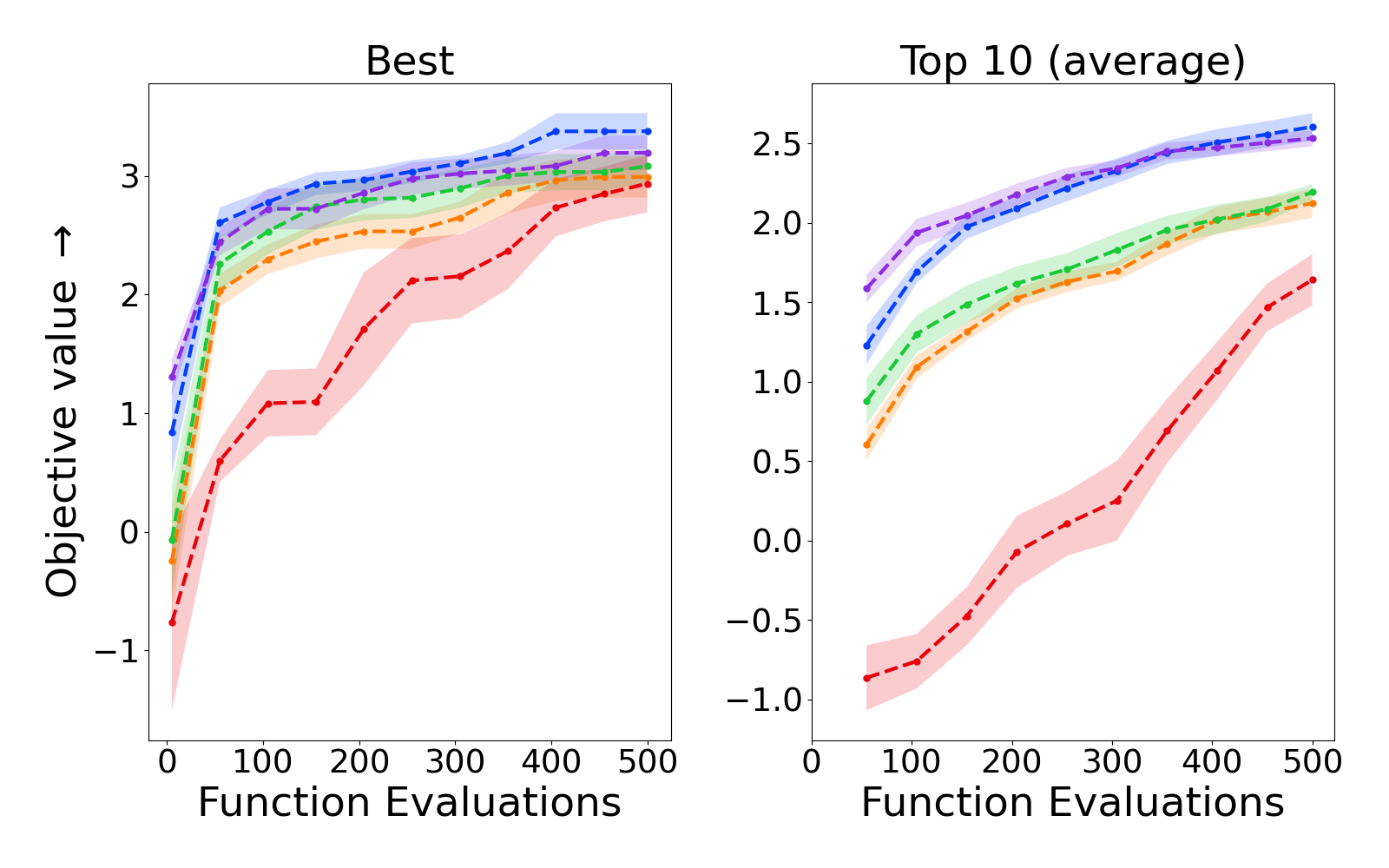
(b) logP optimization over molecules.

Figure 2: BO performance on the expressions and logP tasks. For each method, the best performing parameter on the top 10 average task is displayed. Shaded regions correspond to one standard deviation calculated over 10 independent runs. ScaLES achieves strong performance in both tasks.

4.2.2 Guacamol benchmarks with SELFIES VAE

The Guacamol benchmark suite (Brown et al., 2019) provides a set of de-novo molecular design tasks. For each task an oracle function is provided with scores that are normalized to be between 0 and 1.

Optimization tasks

Following Maus et al. (2022), we consider the objectives: Perindopril MPO, Ranolazine MPO, and Zaleplon MPO. These relate to drugs for high blood pressure, chest pain, and insomnia. We use the pre-trained SELFIES VAE Maus et al. (2022). For each task, we initialize the BO with 1,000 randomly selected training set data points, encoded into the latent space with their objective values. We perform 250 steps of BO with a learning rate of 1, adopting the validity notion of Example 1.3.

Optimization results

Figure 3 shows the cumulative best solution and the average of the top 10, among solutions passing quality filters, across BO steps for the three Guacamol benchmarks. Table 3 displays the relationship between the regularization strength and the percentage of valid solutions generated during BO. Increasing the regularization strength results in significantly more valid solutions generated for all three tasks.

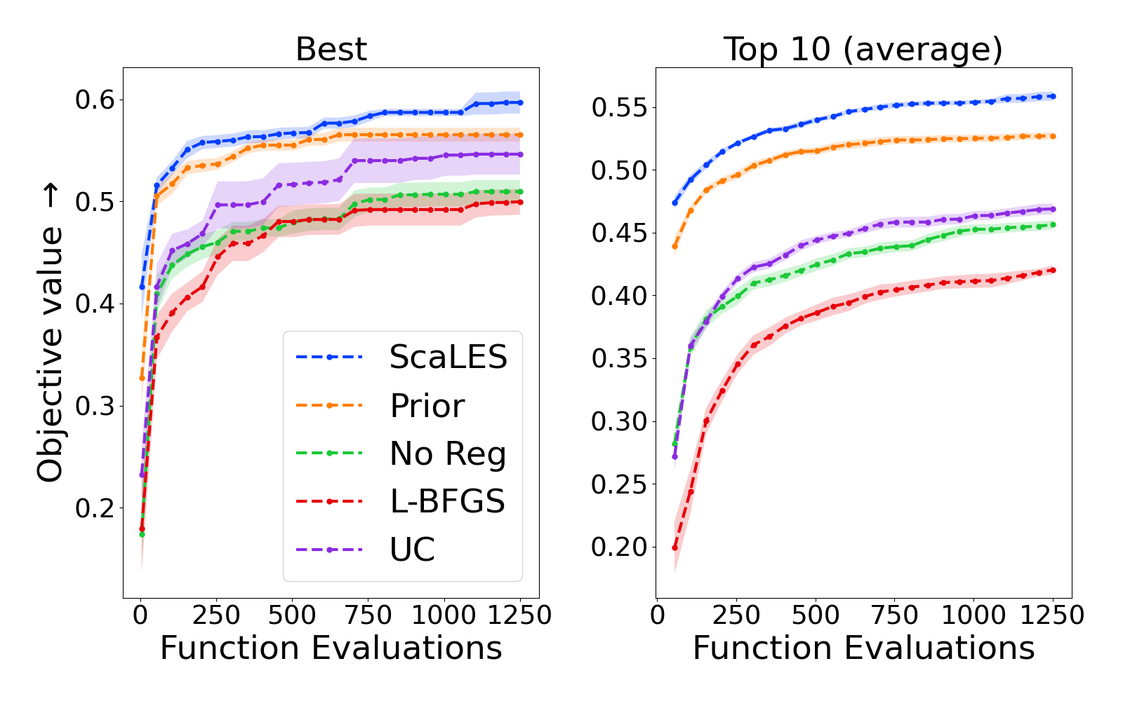
(a) Perindopril MPO

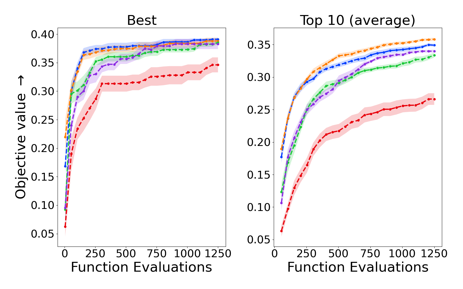
(b) Ranolazine MPO

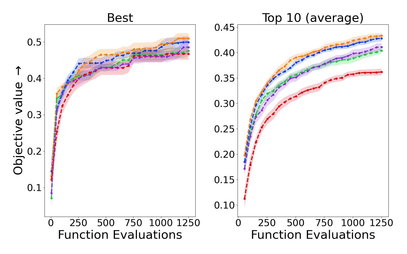
(c) Zaleplon MPO

Figure 3: BO optimization results for the Guacamol benchmark tasks. We visualize the best and the average of top 10 solutions found among those passing the rd_filters quality filters. For each method, the best performing parameter on the top 10 average task is displayed. Shaded regions correspond to one standard deviations calculated over 10 independent runs.

Table 3: The percentage of valid solutions generated through the BO procedure for Guacamol tasks, as studied in 18, is reported. For all tasks, 1,250 solutions are generated during the entire optimization process. Regularization using ScaLES significantly increases the validity of the generated solutions.

Method	Regularization	Ranolazine MPO	Perindopril MPO	Zaleplon MPO
LSO (GA)		26% (1.1)	47% (1)	54% (0.7)
ScaLES	0.2	28% (1.3)	56% (0.5)	62% (0.7)
	0.5	46% (0.7)	70% (0.3)	70% (1)
	0.8	58% (0.7)	78% (0.6)	77% (0.8)
UC	75th quantile	28% (1.1)	46% (1)	54% (0.5)
	95th quantile	26% (1)	46% (1)	55% (0.8)
	100th quantile	28% (1)	47% (2)	54% (0.8)

5 Discussion

We proposed ScaLES, an exact and theoretically motivated method to mitigate over-exploration in LSO. ScaLES is differentiable, fully parallelizable, and scales to large VAEs. Our extensive evaluation shows that penalizing with ScaLES in LSO consistently improves solution quality and objective values. Additionally, ScaLES compares favorably to alternative regularization methods, proving to be the most robust across datasets and various validity notions.

Derived from the density function of a random variable under the decoder transformation, ScaLES serves as a natural out-of-distribution score. A promising future direction is to leverage ScaLES for identifying out-of-distribution data points in deep generative models.

While ScaLES is fully parallelizable, it requires calculating the pseudo-inverse of the Jacobian matrix. This step can become a computational bottleneck when generating long sequences with a large vocabulary. It is left for future work to develop a fast approximation for this operation in order to enable the use of ScaLES in applications involving large language models.

Appendix A Proofs

Lemma A.1.

Let $f_{\theta}$ be a DGN as defined in Equation 8 and assume that $f_{\theta}$ can be expressed as a CPA (Equation 5) and is inevitable, then

$$J{f^{-1}_{\theta}}(\bm{x}) =\left(\begin{bmatrix}\bm{B}_{1}&\cdots&\bm{0}\\ \vdots&\ddots&\vdots\\ \bm{0}&\cdots&\bm{B}_{\textup{L}}\end{bmatrix}\bm{A}_{\omega}^{\dagger}\right)^{T},$$ (16)

where $\bm{A}_{\omega}^{\dagger}$ is the Moore–Penrose inverse of the slope matrix, at the knot whose image constrains $\bm{x}$, and

$$\bm{B}_{i} =\left(\text{diag}\left(\frac{1}{(\bm{p}^{(i)}_{\bm{z}})_{1}},\dots,\frac{1}{(\bm{p}^{(i)}_{\bm{z}})_{\textup{D}}}\right),\bm{1}\frac{1}{c^{(i)}_{\bm{z}}}\right)^{T}.$$ (17)

Proof.

First we write

$$f_{\theta}(\bm{z}) =\text{Softmax}_{+}(\ell_{\theta}(\bm{z})),$$ (18)

Where $\text{Softmax}_{+}$ is the extension of the column wise Softmax function to include the normalizing constants. Specifically, for L by D $\ell_{\theta}(\bm{z})$ matrix, we have

$$\text{Softmax}_{+}(\ell_{\theta}(\bm{z})) =\left(\bm{p}^{(1)}_{\bm{z}},c^{(1)}_{\bm{z}},\dots,\bm{p}^{(L)}_{\bm{z}},c^{(L)}_{\bm{z}}\right)=\bm{x},$$ (19)

with $\bm{p}^{(i)}_{\bm{z}}=(\frac{e^{\ell_{\theta}(\bm{z})_{1i}}}{c^{(i)}_{\bm{z}}})$, and $c^{(i)}_{\bm{z}}=\sum_{j=1}^{\textup{D}}e^{\ell_{\theta}(\bm{z})_{ji}}$.
Next,

$$f_{\theta}^{(-1)}(\bm{x}) =\ell^{-1}_{\theta}(\text{Softmax}_{+}^{-1}(\bm{x}))$$ (20)

A direct calculation yields,

$$\text{Softmax}_{+}^{-1}(\bm{x}) =\left(\log(\bm{p}^{(1)}_{\bm{z}})+\log(c^{(1)}_{\bm{z}}),\dots,\log(\bm{p}^{(L)}_{\bm{z}})+\log(c^{(L)}_{\bm{z}})\right).$$ (21)

As we assume $\ell_{\theta}$ is bijective and can be written as

$$\ell_{\theta}(\bm{z}) =\sum_{\omega\in\Omega}\left(\bm{A}_{\omega}\bm{z}+\bm{b}_{\omega}\right)1_{\bm{z}\in\omega},$$ (22)

we have that

$$\ell^{-1}_{\theta}(\text{Softmax}_{+}^{-1}(\bm{x})) =(\text{Softmax}_{+}^{-1}(\bm{x})-\bm{b}_{\omega})\bm{A}_{\omega}^{\dagger}.$$ (23)

Lastly, as

$$\frac{\partial\text{Softmax}_{+}^{-1}(\bm{x})}{\partial\bm{x}} =\begin{bmatrix}\bm{B}_{1}&\cdots&\bm{0}\\ \vdots&\ddots&\vdots\\ \bm{0}&\cdots&\bm{B}_{\textup{L}}\end{bmatrix},$$ (24)

for

$$\bm{B}_{i} =\left(\text{diag}\left(\frac{1}{(\bm{p}^{(i)}_{\bm{z}})_{1}},\dots,\frac{1}{(\bm{p}^{(i)}_{\bm{z}})_{\textup{D}}}\right),\bm{1}\frac{1}{c^{(i)}_{\bm{z}}}\right)^{T}.$$ (25)

we obtain the final result. ∎

Proof of Theorem 3.1.

First, we note that by our invertability assumption we have that $\mathbb{P}(\bm{x}\in W)=\mathbb{P}(\bm{z}\in f_{\theta}^{(-1)}(W))$. We then proceed with a direct calculation

$$\mathbb{P}(\bm{x}\in W) =\mathbb{P}(\bm{z}\in f_{\theta}^{(-1)}(W))$$ (26)

$$=\sum_{\omega\in\Omega}\mathbb{P}(\bm{z}\in(f_{\theta}^{(-1)}(W)\cap\omega))$$ (27)

$$=\sum_{\omega\in\Omega}\intop_{f_{\theta}^{(-1)}(W)\cap\omega}f_{\bm{z}}(\bm{z})d\bm{z}$$ (28)

$$=\sum_{\omega\in\Omega}\intop_{W\cap f_{\theta}(\omega)}f_{\bm{z}}(f_{\theta}^{(-1)}(\bm{x}))\sqrt{\det{\left(Jf_{\theta}^{(-1)}(\bm{x})Jf_{\theta}^{(-1)}(\bm{x})^{T}\right)}}d\bm{x}$$ (29)

$$=\intop_{W}\sum_{\omega\in\Omega}f_{\bm{z}}(f_{\theta}^{(-1)}(\bm{x}))\sqrt{\det{\left(Jf_{\theta}^{(-1)}(\bm{x})Jf_{\theta}^{(-1)}(\bm{x})^{T}\right)}}1_{\{\bm{x}\in f_{\theta}(\omega)\}}d\bm{x}.$$ (30)

Using Lemma A.1, we get that the volume element is

$$Jf_{\theta}^{(-1)}(\bm{x})Jf_{\theta}^{(-1)}(\bm{x})^{T} =\left(\begin{bmatrix}\bm{B}_{1}&\cdots&\bm{0}\\ \vdots&\ddots&\vdots\\ \bm{0}&\cdots&\bm{B}_{\textup{L}}\end{bmatrix}\bm{A}_{\omega}^{\dagger}\right)^{T}\left(\begin{bmatrix}\bm{B}_{1}&\cdots&\bm{0}\\ \vdots&\ddots&\vdots\\ \bm{0}&\cdots&\bm{B}_{\textup{L}}\end{bmatrix}\bm{A}_{\omega}^{\dagger}\right)$$ (31)

$$\left((\bm{A}_{\omega}^{\dagger})^{T}\begin{bmatrix}\bm{B}_{1}^{T}&\cdots&\bm{0}\\ \vdots&\ddots&\vdots\\ \bm{0}&\cdots&\bm{B}_{\textup{L}}^{T},\end{bmatrix}\right)\left(\begin{bmatrix}\bm{B}_{1}&\cdots&\bm{0}\\ \vdots&\ddots&\vdots\\ \bm{0}&\cdots&\bm{B}_{\textup{L}}\end{bmatrix}\bm{A}_{\omega}^{\dagger}\right)$$ (32)

$$=\sum_{i=1}^{\textup{L}}(\bm{A}^{\dagger}_{i})^{T}(\bm{B}_{i})^{T}\bm{B}_{i}\bm{A}^{\dagger}_{i},$$ (33)

where $\bm{A}^{\dagger}_{i}=\left(\bm{A}^{(1)}_{\omega},\dots,\bm{A}^{(L)}_{\omega}\right)^{\dagger}_{(i\cdot\textup{D}):(i+1\cdot\textup{D}).}$. ∎

Appendix B Additional experimental details

B.1 Datasets characteristics

Table 4 provides the details of the LSO tasks studies in this paper. For the expression taks we optimize for the negative RMSE for any given expression to 1/3 + x + sin(x * x) measured using 1000 equality spaced points between -10 and 10 Kusner et al. [2017]. The logP values are calculated using the model developed by Wildman and Crippen [1999] and last three tasks use oracle function provided by the GuacaMol Brown et al. [2019] package.

Table 4: Characteristics of the LSO problems provided in this study. We train VAEs following the exact specification in Notin et al. [2021] for the first two tasks. For the remaining tasks, we use the pre-trained VAE provided by Maus et al. [2022]. L and D refer the maximal sequence length and the dimension of the one-hot vectors respectively.

Pre-training Dataset	Black-Box Objective	DGN (latent dimension)	L/ D	Architecture
Expressions 15	1/3 + x + sin(x * x)	CVAE (25) 15	19/15	GRU (RNN)
ZINC 12	penalized logP	CVAE (56) 15	120/35	GRU (RNN)
Guacamol 5	Perindopril MPO	SELFIES-VAE (256) 18	70/97	Transformer
Guacamol 5	Ranolazine MPO	SELFIES-VAE (256) 18	70/97	Transformer
Guacamol 5	Zaleplon MPO	SELFIES-VAE (256) 18	70/97	Transformer

B.2 Full experimental results

We provide the full experimental results for the experiments carried out in Section 4. For each task we report the best and the average of the top 10 solutions found throughout the entire optimization procedure. In addition we report the proportion of valid solutions and the average ScaLES value across the entire optimization procedure.

B.3 Expressions

Reg Method	Reg Param	Validity	ScaLES	Top 1 (Valid)	Top 10 (Valid)
LSO (GA)	N/A	0.70 (0.01)	384.48 (0.74)	-0.36 (0.04)	-0.53 (0.02)
LSO (L-BFGS)	facet length = 1.0	0.88 (0.02)	385.54 (1.32)	-0.38 (0.05)	-0.64 (0.09)
LSO (L-BFGS)	facet length = 5.0	0.86 (0.02)	381.70 (1.54)	-0.32 (0.03)	-0.56 (0.06)
LSO (L-BFGS)	facet length = 25.0	0.90 (0.00)	381.97 (2.01)	-0.39 (0.00)	-0.54 (0.03)
Prior	$\lambda=0.2$	0.66 (0.01)	382.16 (0.97)	-0.38 (0.02)	-0.63 (0.03)
Prior	$\lambda=0.5$	0.56 (0.02)	376.05 (1.18)	-0.45 (0.04)	-0.95 (0.08)
Prior	$\lambda=0.8$	0.47 (0.02)	372.04 (0.64)	-0.67 (0.11)	-1.32 (0.17)
UC	75th quantile	1.00 (0.00)	391.59 (3.89)	-0.34 (0.03)	-0.56 (0.02)
UC	95th quantile	0.98 (0.00)	383.36 (3.89)	-0.36 (0.02)	-0.53 (0.01)
UC	100th quantile	0.76 (0.01)	364.63 (3.95)	-0.36 (0.03)	-0.54 (0.02)
ScaLES	$\lambda=0.2$	0.87 (0.01)	384.11 (4.65)	-0.27 (0.06)	-0.49 (0.02)
ScaLES	$\lambda=0.5$	0.92 (0.01)	401.00 (5.17)	-0.32 (0.05)	-0.52 (0.02)
ScaLES	$\lambda=0.8$	0.93 (0.00)	406.68 (5.33)	-0.32 (0.05)	-0.56 (0.02)
ScaLES	$\lambda=2$	0.95 (0.00)	444.72 (0.27)	-0.44 (0.01)	-0.83 (0.02)
ScaLES (ES)	25th quantile	0.92 (0.00)	409.79 (0.27)	-0.34 (0.02)	-0.51 (0.01)
ScaLES (ES)	50th quantile	0.94 (0.00)	412.93 (0.44)	-0.31 (0.03)	-0.53 (0.01)
ScaLES (ES)	75th quantile	0.95 (0.00)	416.98 (0.32)	-0.38 (0.01)	-0.57 (0.01)

B.4 logP

Reg Method	Reg Param	Validity	ScaLES	Top 1 (Valid)	Top 10 (Valid)
LSO (GA)	N/A	0.19 (0.01)	1.69 (0.003)	3.01 (0.14)	2.15 (0.09)
LSO (L-BFGS)	facet length = 1.0	0.1 (0.01)	0.8 (0.16)	2.63 (0.19)	1.06 (0.19)
LSO (L-BFGS)	facet length = 5.0	0.11 (0.01)	-4.476 (1.717)	2.54 (0.18)	1.26 (0.12)
LSO (L-BFGS)	facet length = 25.0	0.13 (0.007)	-7.583 (2.01)	2.94 (0.24)	1.64 (0.16)
Prior	$\lambda=0.2$	0.19 (0.01)	1.70 (0.003)	2.95 (0.19)	2.09 (0.10)
Prior	$\lambda=0.5$	0.18 (0.01)	1.69 (0.003)	2.82 (0.18)	2.04 (0.11)
Prior	$\lambda=0.8$	0.15 (0.01)	1.69 (0.003)	2.79 (0.11)	1.99 (0.10)
UC	75th quantile	0.70 (0.01)	1.76 (0.004)	3.20 (0.15)	2.53 (0.05)
UC	95th quantile	0.70 (0.01)	1.76 (0.004)	3.20 (0.15)	2.53 (0.05)
UC	100th quantile	0.70 (0.01)	1.76 (0.004)	3.20 (0.15)	2.53 (0.05)
ScaLES	$\lambda=0.2$	0.23 (0.01)	1.72 (0.004)	3.03 (0.23)	2.12 (0.10)
ScaLES	$\lambda=0.5$	0.28 (0.01)	1.76 (0.004)	3.16 (0.13)	2.38 (0.09)
ScaLES	$\lambda=0.8$	0.35 (0.01)	1.79 (0.004)	3.38 (0.15)	2.60 (0.09)
ScaLES	$\lambda=2$	0.47 (0.01)	1.84 (0.004)	3.08 (0.1)	2.53 (0.05)
ScaLES (ES)	25th quantile	0.37 (0.01)	1.71 (0.003)	3.24 (0.11)	2.56 (0.07)
ScaLES (ES)	50th quantile	0.53 (0.01)	1.74 (0.002)	3.17 (0.11)	2.53 (0.04)
ScaLES (ES)	75th quantile	0.62 (0.01)	1.75 (0.002)	3.21 (0.11)	2.62 (0.04)

B.5 Ranolazine MPO

Reg Method	Reg Param	Validity	ScaLES	Top 1 (Valid)	Top 10 (Valid)
LSO (GA)	N/A	0.26 (0.01)	-15.52 (0.36)	0.39 (0.00)	0.36 (0.00)
LSO (L-BFGS)	facet length = 1.0	0.16 (0.01)	-927.47 (25.3)	0.34 (0.01)	0.29 (0.01)
LSO (L-BFGS)	facet length = 5.0	0.26 (0.01)	-11847.16 (940.92)	0.34 (0.01)	0.29 (0.01)
LSO (L-BFGS)	facet length = 10.0	0.31 (0.01)	-27674.82 (2916.84)	0.35 (0.01)	0.30 (0.01)
Prior	$\lambda=0.2$	0.27 (0.01)	0.43 (0.28)	0.39 (0.01)	0.36 (0.00)
Prior	$\lambda=0.5$	0.39 (0.02)	10.38 (2.19)	0.39 (0.01)	0.37 (0.00)
Prior	$\lambda=0.8$	0.55 (0.01)	21.18 (0.21)	0.38 (0.01)	0.37 (0.00)
UC	75th quantile	0.22 (0.01)	-14.51 (1.19)	0.38 (0.01)	0.36 (0.01)
UC	95th quantile	0.22 (0.01)	-14.66 (0.28)	0.38 (0.01)	0.36 (0.00)
UC	100th quantile	0.21 (0.01)	-13.67 (2.27)	0.39 (0.01)	0.35 (0.01)
ScaLES	$\lambda=0.2$	0.28 (0.01)	0.25 (0.68)	0.38 (0.01)	0.34 (0.00)
ScaLES	$\lambda=0.5$	0.47 (0.01)	16.38 (0.25)	0.39 (0.00)	0.37 (0.00)
ScaLES	$\lambda=0.8$	0.58 (0.01)	23.85 (0.08)	0.37 (0.01)	0.35 (0.00)

B.6 Zaleplon MPO

Reg Method	Reg Param	Validity	ScaLES	Top 1 (Valid)	Top 10 (Valid)
LSO (GA)	N/A	0.54 (0.01)	-14.20 (0.58)	0.46 (0.02)	0.38 (0.01)
LSO (L-BFGS)	facet length = 1.0	0.40 (0.01)	-467.28 (25.62)	0.46 (0.02)	0.35 (0.01)
LSO (L-BFGS)	facet length = 5.0	0.40 (0.01)	-5160.41 (962.80)	0.45 (0.02)	0.32 (0.01)
LSO (L-BFGS)	facet length = 10.0	0.40 (0.01)	-9808.73 (1536.68)	0.43 (0.02)	0.32 (0.01)
Prior	$\lambda=0.2$	0.58 (0.01)	1.23 (0.66)	0.48 (0.02)	0.42 (0.01)
Prior	$\lambda=0.5$	0.64 (0.01)	15.67 (0.27)	0.46 (0.01)	0.41 (0.00)
Prior	$\lambda=0.8$	0.73 (0.01)	22.56 (0.11)	0.46 (0.01)	0.40 (0.01)
UC	75th quantile	0.55 (0.01)	-12.85 (0.72)	0.44 (0.01)	0.38 (0.01)
UC	95th quantile	0.56 (0.01)	-11.95 (0.73)	0.48 (0.03)	0.39 (0.02)
UC	100th quantile	0.54 (0.01)	-10.03 (0.56)	0.48 (0.04)	0.39 (0.01)
ScaLES	$\lambda=0.2$	0.62 (0.01)	2.40 (0.62)	0.48 (0.01)	0.41 (0.00)
ScaLES	$\lambda=0.5$	0.69 (0.01)	13.78 (1.66)	0.45 (0.02)	0.40 (0.01)
ScaLES	$\lambda=0.8$	0.76 (0.02)	24.73 (0.16)	0.41 (0.01)	0.35 (0.01)

B.7 Perindopril MPO

Reg Method	Reg Param	Validity	ScaLES	Top 1 (Valid)	Top 10 (Valid)
LSO (GA)	N/A	0.47 (0.01)	-13.6 (0.12)	0.51 (0.01)	0.48 (0.01)
LSO (L-BFGS)	facet length = 1.0	0.23 (0.01)	-1491 (96)	0.48 (0.01)	0.42 (0.01)
LSO (L-BFGS)	facet length = 5.0	0.33 (0.02)	-12304 (1553)	0.51 (0.01)	0.42 (0.00)
LSO (L-BFGS)	facet length = 10.0	0.34 (0.01)	-26359 (3484)	0.50 (0.01)	0.42 (0.00)
Prior	$\lambda=0.2$	0.54 (0.01)	2.1 (0.15)	0.56 (0.02)	0.52 (0.01)
Prior	$\lambda=0.5$	0.67 (0.01)	16.56 (0.13)	0.56 (0.01)	0.54 (0.00)
Prior	$\lambda=0.8$	0.76 (0.01)	22.86 (0.06)	0.57 (0.01)	0.54 (0.00)
UC	75th quantile	0.46 (0.01)	-11.96 (0.26)	0.55 (0.02)	0.49 (0.01)
UC	95th quantile	0.46 (0.01)	-12.01 (0.32)	0.53 (0.02)	0.48 (0.01)
UC	100th quantile	0.47 (0.01)	-11.8 (0.45)	0.52 (0.02)	0.48 (0.01)
ScaLES	$\lambda=0.2$	0.56 (0.01)	1.4 (0.56)	0.59 (0.02)	0.52 (0.01)
ScaLES	$\lambda=0.5$	0.70 (0.00)	16.88 (0.19)	0.59 (0.01)	0.55 (0.00)
ScaLES	$\lambda=0.8$	0.78 (0.01)	24.03 (0.12)	0.60 (0.01)	0.56 (0.01)

Appendix C Computational times and resources

Resources and wall clock times

All the experiments in this works were carried out using a single GPU (NVIDIA A100). Table 5 shows the wall clock running time of calculating ScaLES and its derivative for each one of the datasets studied in this paper.

Table 5: Wall clock times in seconds for different $\bm{z}$ batch sizes and datasets (latent dim in parentheses). The methods evaluated include ScaLES, ScaLES Derivative, and UC. For UC, the number of weights and importance samples are in parentheses.

	Expressions (25)		Smiles (56)		Selfies (256)
	Batch 10	Batch 5	Batch 10	Batch 5	Batch 10	Batch 5
ScaLES	0.133	0.04	0.277	0.219	8.687	4.491
ScaLES Derivative	0.18	0.085	0.417	0.369	8.026	5.4
UC (10, 10)	0.162	0.106	1.041	0.841	13.177	12.649
UC (2, 2)	0.021	0.021	0.169	0.159	2.549	2.469

Software packages used

In this work we used the following software packages:

• https://github.com/pascalnotin/uncertainty_guided_optimization Notin et al. [2021]

• https://github.com/nataliemaus/lolbo Maus et al. [2022]

• BoTorch Balandat et al. [2020]

• PyTorch Paszke et al. [2017]

Appendix D Broader impact

This work seeks to improve the practicality of latent space optimization, a method first used in drug discovery. It brings no new societal implications beyond those already associated with LSO.

References

- Ament et al. (2024) Sebastian Ament, Samuel Daulton, David Eriksson, Maximilian Balandat, and Eytan Bakshy. Unexpected improvements to expected improvement for bayesian optimization. Advances in Neural Information Processing Systems, 36, 2024.
- Baell and Holloway (2010) Jonathan B Baell and Georgina A Holloway. New substructure filters for removal of pan assay interference compounds (pains) from screening libraries and for their exclusion in bioassays. Journal of medicinal chemistry, 53(7):2719–2740, 2010.
- Balandat et al. (2020) Maximilian Balandat, Brian Karrer, Daniel R. Jiang, Samuel Daulton, Benjamin Letham, Andrew Gordon Wilson, and Eytan Bakshy. BoTorch: A Framework for Efficient Monte-Carlo Bayesian Optimization. In Advances in Neural Information Processing Systems 33, 2020. URL http://arxiv.org/abs/1910.06403.
- Balestriero and Baraniuk (2018) Randall Balestriero and Richard Baraniuk. Mad max: Affine spline insights into deep learning. arXiv preprint arXiv:1805.06576, 2018.
- Brown et al. (2019) Nathan Brown, Marco Fiscato, Marwin HS Segler, and Alain C Vaucher. Guacamol: benchmarking models for de novo molecular design. Journal of chemical information and modeling, 59(3):1096–1108, 2019.
- Daubechies et al. (2022) Ingrid Daubechies, Ronald DeVore, Nadav Dym, Shira Faigenbaum-Golovin, Shahar Z Kovalsky, Kung-Chin Lin, Josiah Park, Guergana Petrova, and Barak Sober. Neural network approximation of refinable functions. IEEE Transactions on Information Theory, 69(1):482–495, 2022.
- Frazier (2018) Peter I Frazier. Bayesian optimization. In Recent advances in optimization and modeling of contemporary problems, pages 255–278. Informs, 2018.
- Gómez-Bombarelli et al. (2018) Rafael Gómez-Bombarelli, Jennifer N Wei, David Duvenaud, José Miguel Hernández-Lobato, Benjamín Sánchez-Lengeling, Dennis Sheberla, Jorge Aguilera-Iparraguirre, Timothy D Hirzel, Ryan P Adams, and Alán Aspuru-Guzik. Automatic chemical design using a data-driven continuous representation of molecules. ACS central science, 4(2):268–276, 2018.
- Griffiths and Hernández-Lobato (2020) Ryan-Rhys Griffiths and José Miguel Hernández-Lobato. Constrained bayesian optimization for automatic chemical design using variational autoencoders. Chemical science, 11(2):577–586, 2020.
- Humayun et al. (2021) Ahmed Imtiaz Humayun, Randall Balestriero, and Richard Baraniuk. Magnet: Uniform sampling from deep generative network manifolds without retraining. In International Conference on Learning Representations, 2021.
- Humayun et al. (2022) Ahmed Imtiaz Humayun, Randall Balestriero, and Richard Baraniuk. Polarity sampling: Quality and diversity control of pre-trained generative networks via singular values. In Proceedings of the IEEE/CVF Conference on Computer Vision and Pattern Recognition, pages 10641–10650, 2022.
- Irwin et al. (2012) John J Irwin, Teague Sterling, Michael M Mysinger, Erin S Bolstad, and Ryan G Coleman. Zinc: a free tool to discover chemistry for biology. Journal of chemical information and modeling, 52(7):1757–1768, 2012.
- Jin et al. (2018) Wengong Jin, Regina Barzilay, and Tommi Jaakkola. Junction tree variational autoencoder for molecular graph generation. In International conference on machine learning, pages 2323–2332. PMLR, 2018.
- Krenn et al. (2020) Mario Krenn, Florian Häse, AkshatKumar Nigam, Pascal Friederich, and Alan Aspuru-Guzik. Self-referencing embedded strings (selfies): A 100% robust molecular string representation. Machine Learning: Science and Technology, 1(4):045024, 2020.
- Kusner et al. (2017) Matt J Kusner, Brooks Paige, and José Miguel Hernández-Lobato. Grammar variational autoencoder. In International conference on machine learning, pages 1945–1954. PMLR, 2017.
- Lipinski et al. (1997) Christopher A Lipinski, Franco Lombardo, Beryl W Dominy, and Paul J Feeney. Experimental and computational approaches to estimate solubility and permeability in drug discovery and development settings. Advanced drug delivery reviews, 23(1-3):3–25, 1997.
- Liu and Nocedal (1989) Dong C Liu and Jorge Nocedal. On the limited memory bfgs method for large scale optimization. Mathematical programming, 45(1):503–528, 1989.
- Maus et al. (2022) Natalie Maus, Haydn Jones, Juston Moore, Matt J Kusner, John Bradshaw, and Jacob Gardner. Local latent space bayesian optimization over structured inputs. Advances in neural information processing systems, 35:34505–34518, 2022.
- Notin et al. (2021) Pascal Notin, José Miguel Hernández-Lobato, and Yarin Gal. Improving black-box optimization in vae latent space using decoder uncertainty. In M. Ranzato, A. Beygelzimer, Y. Dauphin, P.S. Liang, and J. Wortman Vaughan, editors, Advances in Neural Information Processing Systems, volume 34, pages 802–814. Curran Associates, Inc., 2021. URL https://proceedings.neurips.cc/paper/2021/file/06fe1c234519f6812fc4c1baae25d6af-Paper.pdf.
- Paszke et al. (2017) Adam Paszke, Sam Gross, Soumith Chintala, Gregory Chanan, Edward Yang, Zachary DeVito, Zeming Lin, Alban Desmaison, Luca Antiga, and Adam Lerer. Automatic differentiation in pytorch. 2017.
- Tripp et al. (2020) Austin Tripp, Erik Daxberger, and José Miguel Hernández-Lobato. Sample-efficient optimization in the latent space of deep generative models via weighted retraining. Advances in Neural Information Processing Systems, 33:11259–11272, 2020.
- Walters (2019) P. Walters. rd filters, 2019. URL https://github.com/PatWalters/rd_filters. Accessed: January 14, 2019.
- Wildman and Crippen (1999) Scott A Wildman and Gordon M Crippen. Prediction of physicochemical parameters by atomic contributions. Journal of chemical information and computer sciences, 39(5):868–873, 1999.