Reinforced Decoder: Towards Training Recurrent Neural Networks for Time Series Forecasting

Abstract

Recurrent neural network-based sequence-to-sequence models have been extensively applied for multi-step-ahead time series forecasting. These models typically involve a decoder trained using either its previous forecasts or the actual observed values as the decoder inputs. However, relying on self-generated predictions can lead to the rapid accumulation of errors over multiple steps, while using the actual observations introduces exposure bias as these values are unavailable during the extrapolation stage. In this regard, this study proposes a novel training approach called reinforced decoder, which introduces auxiliary models to generate alternative decoder inputs that remain accessible when extrapolating. Additionally, a reinforcement learning algorithm is utilized to dynamically select the optimal inputs to improve accuracy. Comprehensive experiments demonstrate that our approach outperforms representative training methods over several datasets. Furthermore, the proposed approach also exhibits promising performance when generalized to self-attention-based sequence-to-sequence forecasting models.

I Introduction

Multi-step-ahead time series prediction, which involves extrapolating a sequence of future values based on historical observations, plays a vital role in various real-world fields, such as economics [1], energy [2, 3], and climate [4, 5]. Over the past few decades, considerable research efforts have been devoted to developing statistical and machine learning techniques for multi-step-ahead time series forecasting [6, 7, 8, 9, 10]. Among these techniques, recurrent neural networks (RNNs) have achieved notable success due to their capacity to characterize temporal patterns in sequential data [10, 11, 12]. Inspired by the remarkable progress in neural machine translation, sequence-to-sequence (S2S) models have been widely applied in various time series forecasting applications [4, 5, 13, 14]. The S2S models typically consist of two independent RNNs, serving as the encoder and decoder, respectively. The encoder transforms the input sequence of historical observations into latent representations. The decoder generates the output sequence auto-regressively, where each prediction at the subsequent step is yielded based on the self-generated output from the previous step.

As for training the S2S models, the most fundamental strategy is free running (FR) [15, 4]. Under the FR strategy (Fig. 1), the training process remains consistent with the extrapolating process, i.e., feeding back the one-step-ahead prediction to the decoder to predict the value at the next step. However, this strategy suffers from error accumulation over time, as the feedback loop magnifies the initial errors. Accordingly, some non-autoregressive architectures were proposed to obviate the error propagation issue [10, 16, 17]. For instance, Hewamalage et al. [10] used a dense layer to directly project the output of the last encoder time step to the desired forecast horizon. Although bypassing error propagation, such non-autoregressive architectures might have limited capacity to characterize the temporal relationships among multiple time steps [15].

In contrast to the FR strategy, an alternative training strategy, namely teacher forcing (TF), is proposed by using the ground truth values as the inputs to the decoder during the training stage. This strategy breaks the feedback loop and forces the output sequence to remain as close as possible to the ground truth sequence [18]. Nevertheless, as the true values are not available when extrapolating, the decoder still has to produce predictions based on feeding back the one-step-ahead prediction. This discrepancy between training and extrapolation stages, which is referred to as exposure bias [19], can lead to poor performance [19, 20, 21].

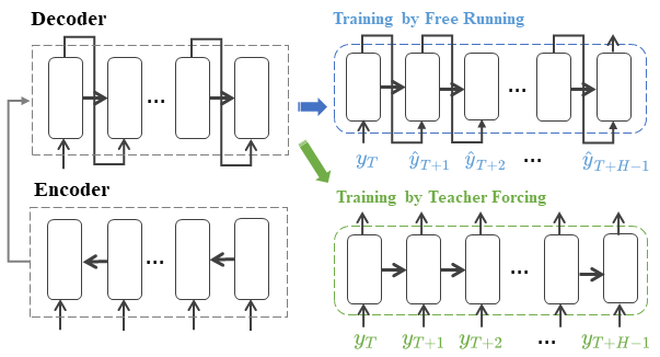
Figure 1: Sequence-to-sequence (S2S) model. $\left\{\hat{y}_{T+1},...,\hat{y}_{T+H}\right\}$ denotes the $H$-step-ahead prediction sequence and $\left\{y_{T},...,y_{T+H}\right\}$ denotes the sequence of the corresponding observations.

In order to alleviate exposure bias, plenty of research has been conducted, which can be broadly categorized into two streams. One stream explores the utilization of generative adversarial networks (GANs) to align the hidden states between the training and extrapolation stages over multiple steps [21, 22, 23]. However, these methods suffer from mode collapse inherent in GANs that hinders effective training [24, 25]. The other stream focuses on adjusting the exposure level of the ground truth values in the TF strategy [19, 26, 27]. For example, Taigman et al. [26] proposed a variant of the TF strategy, in which the average of true values and predictions with added random noise are used as the decoder inputs. Bengio et al. [27] designed the scheduled sampling approach, which gradually replaces true values with self-generated outputs based on probability. Nonetheless, these adjustment schemes either introduce new sources of noise or lack adaptability to the dynamic training process. Moreover, prior works have predominantly focused on other sequence modeling tasks, such as machine translation and vocal synthesis, while little attention has been paid to time series forecasting which is the focus of this study.

To this end, a novel framework called reinforced decoder (RD) is proposed for training sequence-to-sequence models in the forecasting field. By introducing a model pool containing several well-trained auxiliary models, the proposed method adopts external predictions as candidate inputs for the decoder. This facilitates the rectification of self-generated inputs that exhibit substantial errors during the auto-regressive process and, thus, mitigates the error accumulation of the decoder. Meanwhile, the availability of candidate inputs throughout both the training and extrapolation stages ensures consistent decoding and circumvents exposure bias. As the optimal input-providing model from the pool will be different, due to changes in data samples, time steps, and training stages [2, 1, 28], rigidly pre-defining a selection scheme based on manual experience or conventional optimization methods seems inadvisable. In this context, the REINFORCE algorithm [29], an efficient approach originating from the reinforcement learning (RL) community, is leveraged to select an optimal candidate input at each time step, considering its advantages in terms of solving sequential decision problems dynamically and adaptively [30, 31, 32]. During both the training and extrapolation stages, the selected input from the best-performing pool member is fed to the decoder, guiding the decoding process for the next time step. The primary contributions of this work are summarized below.

• A novel framework called RD is proposed to train S2S models for multi-step-ahead time series prediction. Under the RD framework, the inputs of the decoder are generated from the same model pool during both the training and extrapolation stages, which helps to circumvent exposure bias.

• A dynamic selection scheme is developed to yield the optimal inputs from the model pool to the decoder. By leveraging the RL algorithm, the input values of the decoder are adaptively corrected by the auxiliary models as best as possible, which contributes to the alleviation of error propagation.

• Extensive experiments were conducted on well-accepted simulated and real-world time-series datasets with different time granularities. The results show that our approach excels over the state-of-the-art counterparts and has a strong generalization capability on different S2S structures.

The rest of this paper is organized as follows. Section II introduces the basic related concepts. Section III details the proposed approach. Then, the experimental settings for the datasets, accuracy measures, and comparison methods are described in Section IV. The experimental results are discussed in Section V, and the conclusions are drawn in Section VI.

II Background Study

II-A Multi-Step-Ahead Time Series Prediction

In the general multi-step-ahead time series forecasting problem, a dataset $D$ contains input–target pairs $(X,\ Y)$, where $X=(X_{1},\ \dots,\ X_{T})\in\mathbb{R}^{T}$ denotes the historical observations with $T$ time lags, and $Y=(y_{T+1},\ \dots,\ y_{T+H})\in\mathbb{R}^{H}$ denotes the corresponding observations in the future over the horizon $H$. The goal of time series prediction is to learn a target function, $\mathcal{F}(\cdot)$, on the dataset that maps the input $X$ to its corresponding target sequence. That is, $\hat{Y}=\mathcal{F}(X)$. As shown in Fig. 1, the RNN-based S2S model generally formulates this function using an encoder–decoder architecture [33]. The encoder introduces a hidden state, $h_{j}$, at each time step $j$, to capture the temporal relationships within the historical time series:

$$h_{j}=f_{e}(h_{j-1},X_{j}),\quad 1\leq j\leq T,$$ (1)

where $f_{e}(\cdot)$ denotes the non-linear activation function inside the encoder, and $X_{j}$ contains the historical observations of the target variate $y_{j}$ and the corresponding covariates. The last $h_{T}$, which summarizes the whole sequence of historical observations, is usually used as the context vector c that is passed to the decoder [5, 17]. Next, in the decoding stage, a decoder is utilized to generate the predictions auto-regressively. Specifically, $\hat{y}_{T+k}$ can be obtained according to the following:

$$s_{k} =f_{d}\left({s}_{k-1},\ \hat{y}_{T+k-1},\ \textbf{\emph{c}}\right),$$ (2)

$$\hat{y}_{T+k} =g\left(s_{k}\right),$$ (3)

where $1\leq k\leq H$, $f_{d}(\cdot)$ denotes the non-linear activation function inside the recurrent units of the decoder, $g(\cdot)$ is the function inside the output layer, and $\hat{y}_{T+k}$ represents the model’s prediction for its corresponding true observation ${y}_{T+k}$ at time step $T+k$.

Common choices for $f_{e}(\cdot)$ and $f_{d}(\cdot)$ include the Elman RNN (ERNN) [34], long short-term memory (LSTM) [35], and gated recurrent unit (GRU) [36]. In this study, we use LSTM to illustrate the mechanism of the proposed reinforced decoder (Fig. 3) [10, 5]. In addition, a state-of-the-art variant of LSTM with embedded hybrid spiking neurons (i.e., ESLSTM [16]) is also used to test the general ability of our method in relation to different recurrent units.

II-B Training Method for Recurrent Neural Networks

Backpropagation is the fundamental algorithm for training neural networks via gradient descent [37]. In an RNN, calculating gradients requires backpropagation through time (BPTT)  [38], due to the sequential nature of forward propagation, which incurs high memory and computational costs. The teacher forcing (TF) strategy was first proposed to avoid BPTT for simple recurrent networks lacking hidden-to-hidden connections [37, 18]. In the TF strategy, the ground truth values are fed as decoder inputs instead of self-generated predictions, decoupling the time steps to allow for parallelized training. Subsequent work extended the TF strategy to more complex recurrent networks containing both hidden-to-hidden and output-to-hidden recurrence [15, 39, 37], such as the decoder shown in Eq. (2)–(3). In these cases, the TF strategy is often combined with BPTT, where BPTT primarily handles hidden-to-hidden recurrence, and TF is used for output-to-hidden recurrence. This combination enables the model to capture long-term dependencies while reducing the computational costs associated with full BPTT. However, as true values are unavailable when extrapolating, the TF strategy induces exposure bias [19], which can lead to poor performance [15].

In order to mitigate the exposure bias of TF, Lamb et al. [21] proposed the professor forcing (PF) method, which used generative adversarial networks (GANs) to align the hidden states between the training and extrapolation stages over multiple steps. Subsequently, many variants of the PF method have been derived [22, 23]. However, these methods suffer from mode collapse, which is inherent to GANs and hinders effective training [24, 25]. Hence, more general methods adjust the exposure level of the ground truth values in TF [13, 10]. For example, Taigman et al. [26] proposed a variant of the TF technique, which uses the average of true values and predictions with added noise as the decoder input. Bengio et al. [27] designed a scheduled sampling approach, gradually replacing true values with self-generated outputs based on probability. However, existing adjustment schemes either introduce new sources of noise or lack adaptability to the dynamic training process. Furthermore, previous research has mainly focused on machine translation and vocal synthesis, with little attention being paid to time series forecasting. Thus, this study introduces auxiliary models and the reinforcement learning method to enable dynamic and adaptive guidance (i.e., input) control of the decoder in the context of multi-step-ahead time series prediction.

II-C Reinforcement Learning

Inspired by the principles of behaviorist psychology, reinforcement learning (RL) aims to empower computational agents to learn optimal behaviors through trial-and-error interactions with their environment [32]. With the core objective of maximizing cumulative rewards over time, the RL framework has been successfully applied to many sequential decision-making problems, ranging from game playing to resource management [30, 31, 32]. Specifically, RL lies in the concept of the agent–environment interaction, where, the agent represents the action-maker, and the environment encompasses information external to the agent within the context of the considered problem.

To effectively apply RL algorithms, the problem is usually required to be formulated as a Markov decision process (MDP), which comprises a state space $\mathcal{S}$, an action space $\mathcal{A}$, a state transition function $\mathcal{P}\left(\cdot\right)$ satisfying the Markov property, and a reward calculation function $\mathcal{R}\left(\cdot\right)$. At each step $k$ of the sequential decision problem, the agent perceives the current state $s_{k}$ of the environment and selects an action $a^{\star}_{k}$, according to a mapping from states to actions called the policy. The environment then updates its state based on the transition function and provides a feedback reward to the agent.

Within the framework of RL, the goal of sequential decision-making is shifted from finding an optimal set over all possible sequences of actions to focusing only on the optimal actions under the states, i.e., learning the optimal policy. Therefore, it can lead to more efficient and effective decision-making in complex, dynamic problems, where traditional methods may be limited. Among the categories of RL algorithms, variants of policy gradient (PG) algorithms, which model the policy directly with a parameterized machine learning model, have consistently produced state-of-the-art results [40]. In general, the policy $\pi_{\theta}$ (with parameters $\theta$) is a probability distribution over the actions $a^{j}\in\mathcal{A}$, conditioned on the state $s_{k}$ at step $k$. In the case that a stochastic policy is used, where the action space is discrete, such as the input selection problem for the decoder in this study, the policy can be defined as follows:

$$\pi_{\theta}(a^{j}|s_{k})=P[a^{j}|s_{k};\theta].$$ (4)

In this way, the optimal policy is obtained by optimizing the parameters $\theta$ through gradient ascent with a set of training samples. Among the PG algorithms derived from the policy gradient theorem, REINFORCE is one of the most representative algorithms [29, 30, 31, 32]. In this study, we follow REINFORCE to provide the calculation formula for the gradient.

III Methodology

This section first presents the proposed reinforced decoder. Subsequently, the Markov decision process formulation for the input selection of the decoder is described. Then, the training and construction processes of the S2S model with the reinforced decoder are explained.

III-A The Reinforced Decoder based on Recurrent Neural Networks

As shown in Fig. 3, in contrast to the standard RNN-based S2S model containing solely an encoder and a decoder [33], the proposed reinforced decoder additionally incorporates the agent and a model pool. For the sake of simplicity but without loss of generality, the LSTM unit is used here to compose the S2S model to illustrate the mechanism of the proposed reinforced decoder, for which the forward propagation process is detailed as follows.

Encoder. This reads the historical observations $X_{1:T}$ sequentially and builds the hidden state according to Eq. (1). The last state, $h_{T}\in\mathbb{R}^{N_{e}}$, is used as the context vector c and is passed to the decoder [5, 17].

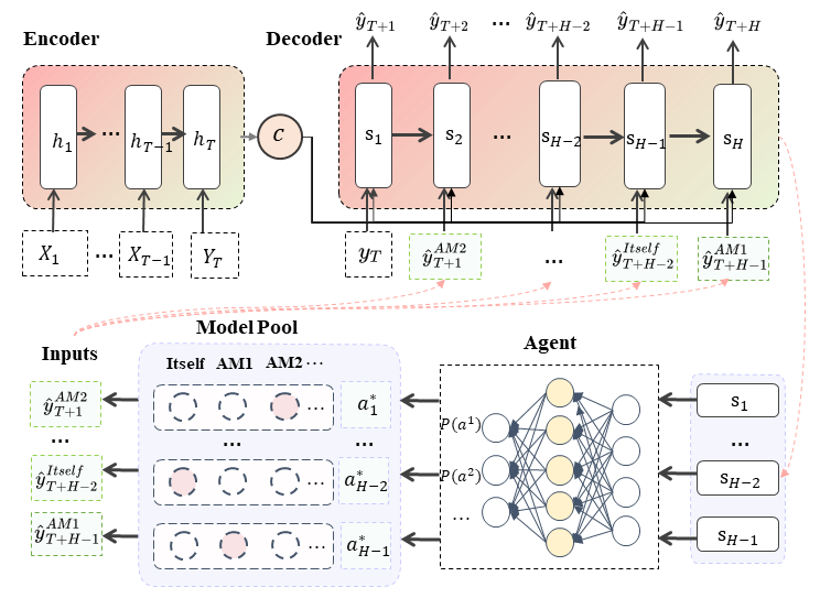
Figure 2: Basic framework of S2S model with reinforced decoder. $\{P(a^{1}),P(a^{2}),...)\}$ is the output of the policy network of the agent, which is the probability value of executing the corresponding action. AM1, AM2 represent the auxiliary models. Itself represents the decoder.

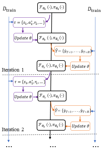
Figure 3: Illustration of asynchronous training.

Reinforced Decoder. This outputs the predictions based on the context vector and the inputs generated by the models in the pool. Specifically, $f_{d}(\cdot)$ and $g(\cdot)$ in Eq. (2)–(3) are summarized as follows:

$$\psi_{k}=\sigma\left(U_{\psi}\left[s_{k-1},\ \varphi_{T+k},\ \textbf{\emph{c}}\right]+b_{\psi}\right),$$ (5)

$$i_{k}=\sigma\left(U_{i}\left[s_{k-1},\ \varphi_{T+k},\ \textbf{\emph{c}}\right]+b_{i}\right),$$ (6)

$$\tilde{c}_{k}=tanh\left(U_{c}\left[s_{k-1},\ \varphi_{T+k},\ \textbf{\emph{c}}\right]+b_{c}\right),$$ (7)

$$c_{k}=i_{k}\odot\tilde{c}_{k}+f_{t}\odot c_{k-1},$$ (8)

$$o_{k}=\sigma\left(U_{o}\left[s_{k-1},\ \varphi_{T+k},\ \textbf{\emph{c}}\right]+b_{o}\right),$$ (9)

$$s_{k}=o_{k}\odot tanh\left(c_{k}\right),$$ (10)

$$\hat{y}_{T+k}=Vs_{k}+b,$$ (11)

where $s_{k},c_{k},\tilde{c}_{k}\in\mathbb{R}^{N_{d}}$ are the hidden state, the cell state, and candidate cell state of the decoder at step $k\in\left\{1,2,...,H\right\}$, respectively; $N$ is the cell dimension; $U_{\psi},U_{i},U_{o},U_{c}\in\mathbb{R}^{N_{d}\times\left(N_{d}+1+N_{e}\right)}$ denote the weight matrices of the forget gate, input gate, output gate, and cell state, respectively, and $b_{\psi},b_{i},b_{o},b_{c}\in\mathbb{R}^{N_{d}}$ denote the corresponding bias vectors; $\psi_{k},i_{k},o_{k}\in\mathbb{R}^{N_{d}}$ are the forget, input, and output gate vectors; $V\in\mathbb{R}^{1\times N_{d}},b\in\mathbb{R}^{1}$ denote the weight matrix and bias vector of the output layer. Note that $\varphi_{T+k}\in\mathbb{R}^{1}$ is the input to the decoder at time step $T+k$, which is denoted as follows:

$${\varphi_{T+k}}=\begin{cases}y_{T},&{k=1},\\ {\hat{y}_{T+k-1}^{a^{\star}_{k-1}},}&{1<k\leq H,}\end{cases}$$ (12)

where $a^{\star}_{k-1}$ denotes the model chosen from the model pool to provide the decoder inputs, and $\hat{y}_{T+k-1}^{a^{\star}_{k-1}}$ represents its forecast of $y_{T+k-1}$. The model pool consists of the decoder itself and auxiliary models.

In this context, the auxiliary models are expected to have the capacity to generate multi-step-ahead predictions without any specific constraints on their internal structure. Consequently, a variety of options is available for auxiliary models, ranging from simple statistical models [6] to more complex machine learning models [7, 8, 9]. In order to strike a balance between computational efficiency and the ability to capture diverse temporal relationships, it is advisable to consider non-autoregressive models with lower computational requirements. The specific auxiliary model chosen can be tailored to the requirements and characteristics of the considered tasks.

Note that we consider two auxiliary models in this study, i.e., well-trained multiple-output support vector regression (MSVR)[8] and multi-layer perception (MLP), in view of their high efficiency and wide application in multi-step time series prediction [41, 2, 1, 42, 3]. In addition, preliminary experimentation revealed that they exhibited superior performance in terms of both computational efficiency and predictive accuracy, compared to other multi-step time series forecasting approaches such as ARIMA [6] and random forest [9].

Given the inherent sequential nature of discerning the optimal model $a^{\star}_{k-1}$, where each selection influences the subsequent predictions of the decoder and choices, the model selection procedure exhibits the characteristics of a sequential decision-making problem [43]. Such sequential decision characteristics, coupled with the inherent uncertainty of an optimal input-providing model, render manual experience or conventional optimization techniques ill-suited for this purpose. Formulating the problem as a framework for sequential decision-making under uncertainty provides a principled approach to address this complexity.

III-B MDP Setting for the Input Selection of the Decoder

Inspired by the remarkable progress of RL in sequential decision-making problems, the REINFORCE algorithm [29] was introduced to solve the decoder input selection problem. As illustrated in Fig. 3, at each step $k\in\left\{1,2,\dots,H-1\right\}$, the agent observes the current decoding situation and selects a model for which the prediction is fed into the decoder. The decoder then transits to the next state and gives a reward to the agent. The specific mathematical model, MDP $\left\langle\mathcal{S},\ \mathcal{A},\ \mathcal{P},\ \mathcal{R}\right\rangle$, is summarized as follows:

State space. Each state is defined as the current hidden state of the decoder (i.e., $s_{k}$), as it stores the decoding status that retains all relevant information for the agent to select actions.

Action space. Each element $a^{j}$ within the action space $\mathcal{A}$ describes the candidate behavioral characteristics of the agent. Here, the action space $\mathcal{A}$ is a set containing the candidate models for generating the predictions (inputs) for the decoder (i.e., the decoder itself and the auxiliary models).

Transition function. As the state is defined as the hidden state of the decoder, its transitions follow Eq. (5)–(12), which can be simplified to $s_{k+1}=\mathcal{F}_{\vartheta}(s_{k},\ a^{\star}_{k})$. $\mathcal{F}_{\vartheta}\left(\cdot\right)$ consists of the encoder LSTM and decoder LSTM, in which $\vartheta$ includes the weight matrices and bias vectors related to the forget gates, input gates, output gates, and the output layer.

Reward function. The reward, $r_{k}$, is a numerical value representing the instant reward to the agent affiliated with executing the action $a^{\star}_{k}$ in state $s_{k}$. As the agent learns through trial and error, the design of the reward function dictates the optimal policy. In this study, it is desired that the decoder generates accurate predictions for the next time step after being fed with the predictions from the model selected by the agent. Therefore, $r_{k}$ is defined as follows [28]:

$$r_{k}=\alpha\cdot\text{\emph{Rank}}_{k}+(1-\alpha)\cdot\text{\emph{Accuracy}}_{k},$$ (13)

where $\alpha$ is a hyperparameter that balances the two types of rewards, $\text{\emph{Rank}}_{k}$ is designed to motivate the agent to select the model with the highest accuracy at step $k$, and $\text{\emph{Accuracy}}_{k}$ evaluates the performance of the decoder at step $k+1$ using the chosen prediction of the model as the input. These terms are defined as follows:

$$\text{\emph{Rank}}_{k}=1-\frac{rank\left(a^{\star}_{k}\right)}{N^{a}},$$ (14)

where $N_{a}$ is the number of actions in the action space $\mathcal{A}$, which is also the number of models in the model pool. The models are rank-ordered from 1 (the best) to $N_{a}$ (the worst),, according to the prediction accuracy. Furthermore, $rank\left(a^{\star}_{k}\right)$ indicates the ordinal number of the model selected by the agent at step $k$.

$$\text{\emph{Accuracy}}_{k}=\frac{\beta}{\beta+\left\lvert y_{T+k+1}-\hat{y}_{T+k+1}\right\rvert},$$ (15)

where $\beta$ is a hyperparameter that converts penalties to reward-based metrics, and $\hat{y}_{T+k+1}$ is the prediction generated by the decoder at step $k+1$ after being fed into the selected input by the agent.

In addition, the policy $\pi_{\theta}(\cdot)$ of the agent in Eq. (4) is modeled using a multi-layer perception (MLP) with a single hidden layer and a softmax activation function [44], as defined below. The parameters $\theta$ encompass the weight matrices and bias vectors in the MLP.

$$\pi_{\theta}(s_{k})\triangleq softmax\left(W_{2}\left(\sigma\left(W_{1}s_{k}+b_{1}\right)\right)+b_{2}\right),$$ (16)

where $W_{1}\in\mathbb{R}^{N_{p}\times N_{d}},\ W_{2}\in\mathbb{R}^{N_{a}\times N_{p}},\ b_{1}\in\mathbb{R}^{N_{p}},b_{2}\in\mathbb{R}^{N_{a}}$ denote the weight matrices and bias vectors of the hidden layer and output layer, respectively, and $N_{p}$ is the number of nodes in the hidden layer. Then, the action (model) taken by the agent at step $k$ is obtained by:

$$a^{\star}_{k}=\underset{a^{j}\in\mathcal{A}}{\arg\max}\,\pi_{\theta}\left(a^{j}\mid s_{k}\right).\\$$ (17)

III-C Training and Prediction

The environment faced by the agent would be time-varying if the encoder and the decoder were updated concurrently with the agent’s learning process. In order to ensure the environment remains stationary that is a crucial condition for convergence guarantees of policy gradient methods [45], we adopt an asynchronous updating strategy for the agent and the encoder–decoder RNNs (Fig. 3). Specifically, the parameters of the policy network ($\pi_{\theta}(\cdot)$) within the agent are held constant when training RNNs ($\mathcal{F}_{\vartheta}(\cdot)$) comprising the encoder and decoder. Conversely, the parameters of the RNNs are fixed during the policy network training. Both $\theta$ and $\vartheta$ are updated in the direction of the performance gradient. Algorithm 1 outlines the training process in detail.

Agent. Let $\tau=\left\{s_{1},\ a^{\star}_{1},\ r_{1},\ \ldots,\ s_{H-1},\ a^{\star}_{H-1},\ r_{H-1}\right\}$ be a trajectory denoting the interactions between the agent and the environment in one complete decoding process. The agent’s goal is to obtain a policy that maximizes the expected total reward along $\tau$, defined as follows:

$$\max J\left(\pi_{\theta}\right) =E_{\tau\sim\pi_{\theta}}\left[R(\tau)\right],$$ (18)

where $R(\tau)=\sum_{k=1}^{H-1}\gamma^{k}r_{k}$ is the cumulative discounted reward from the start state, $\gamma$ is a discount factor so that $0\leq\gamma<1$. $P\left(\tau\right)$ denotes the probability of producing $\tau$ given the policy $\pi_{\theta}$ and encoder-decoder $\mathcal{F}_{\vartheta}$. That is, $P\left(\tau\right)=P_{\mathcal{F}_{\vartheta}}\left(s_{1}\right)\prod_{k=1}^{H-1}\pi_{\theta}\left(a^{\star}_{k}|s_{k}\right)P_{\mathcal{F}_{\vartheta}}\left(s_{k+1}|s_{k},a^{\star}_{k}\right)$. The gradient of the training object for the agent is formulated as follows:

$$\bigtriangledown_{\theta}J\left(\pi_{\theta}\right) =\bigtriangledown_{\theta}\sum_{\tau}P\left(\tau\right)R\left(\tau\right)$$ (19)

$$=\sum_{\tau}P\left(\tau\right)\bigtriangledown_{\theta}\text{log}P\left(\tau\right)R\left(\tau\right).$$

Algorithm 1 Asynchronous Training Algorithm of Encoder–Reinforced Decoder.

1:  Input: the supervision samples $D_{train}=(X^{n},\ Y^{n})_{n=1}^{N}$, well-trained auxiliary models, the hyperparameters of the encoder and decoder RNNs, the policy of agent, and the learning rate $l_{1},l_{2}$.

2:  Initialize the policy network $\pi_{\theta}(\cdot)$ and the RNNs $\mathcal{F}_{\vartheta}(\cdot)$ with random parameters $\theta,\vartheta$.

3:  While not sufficiently good performance or maximum number of iterations do

4:     Fix the parameters $\vartheta$ of the RNNs.

5:     Collect a set of trajectories by executing the current policy $\pi_{\theta}(\cdot)$ with $\epsilon$-greedy strategy.

6:     For each trajectory $\tau_{n}=\left\{s_{1,n},\,a^{\star}_{1,n},\,...,\,r_{H-1,n}\right\}$ do

7:       For $k=1\rightarrow H-1$ do

8:         Calculate $G_{k,n}=\sum_{k^{{}^{\prime}}=k}^{H-1}(\gamma^{k^{{}^{\prime}}-k}r_{k^{{}^{\prime}},n})$.

9:         Calculate $K(\tau_{n})=\gamma^{k}G_{k,n}\bigtriangledown_{\theta}\text{log}\pi_{\theta}(a^{\star}_{k,n}\mid s_{k,n})$.

10:         Update policy: $\theta\leftarrow\theta+\frac{1}{N}l_{1}K(\tau_{n})$.

11:       Endfor

12:     Endfor

13:     Fix parameters $\theta$ of policy.

14:     Calculate a set of prediction sequences by executing the current encoder and decoder $\mathcal{F}_{\vartheta}(\cdot)$ according to Eq. (5)–(11).

15:     For each multi-step-ahead prediction sequence $\hat{Y_{n}}=\hat{y}_{T+1:T+H,\,n}$ do

16:       Calculate $\mathcal{L}(\hat{Y_{n}})=\frac{1}{H}\sum_{k=1}^{H}(y_{T+k,\,n}-\hat{y}_{T+k,\,n})^{2}$.

17:       Update RNNs: $\vartheta\leftarrow\vartheta-\frac{1}{N}l_{2}\bigtriangledown_{\vartheta}\mathcal{L}(\hat{Y_{n}})$.

18:     Endfor

As asynchronous training is used, the RNNs remain unchanged when the policy is updated, which is independent of $\theta$. Both $\bigtriangledown_{\theta}\text{log}P_{\mathcal{F}_{\vartheta}}(s_{1})$ and $\bigtriangledown_{\theta}\text{log}P_{\mathcal{F}_{\vartheta}}\left(s_{k+1}|s_{k},a^{\star}_{k}\right)$ are equal to 0. Then, Eq. (19) can be transformed as follows:

$$\bigtriangledown_{\theta}J\left(\pi_{\theta}\right)=\sum_{\tau}P\left(\tau\right)(\sum_{k=1}^{H-1}\bigtriangledown_{\theta}\text{log}\pi_{\theta}\left(a^{\star}_{k}|s_{k}\right)R\left(\tau\right))$$ (20)

$$=E_{\tau\sim\pi_{\theta}}\bigtriangledown_{\theta}\text{log}\pi_{\theta}\left(a^{\star}_{k}|s_{k}\right)R\left(\tau\right)$$

$$=\frac{1}{N}\sum_{n=1}^{N}\sum_{k=1}^{H-1}(\gamma^{k}\bigtriangledown_{\theta}\text{log}\pi_{\theta}(a^{\star}_{k,n}\mid s_{k,n})\sum_{k^{{}^{\prime}}=k}^{H-1}(\gamma^{k^{{}^{\prime}}-k}r_{k^{{}^{\prime}},n})),$$

where $N$ denotes the number of samples in the training set. $a^{\star}_{k,n}$, $s_{k,n}$, and $\tau_{n}$ represent the corresponding action, state, and trajectory for the sample $n$, respectively. Moreover, we use the $\epsilon$-greedy exploration strategy to execute the actions to jump out of local optimal point during the training process, where the agent executes an action randomly with a certain probability, $\epsilon<1$, instead of the policy-based action. That is,

$${a^{\star}_{k,n}}=\begin{cases}\underset{a^{j}\in A}{\arg\max}\,\pi_{\theta}\left(a^{j}\mid s_{k,n}\right),&1-\epsilon,\\ random~{}a^{j}\in A,&\epsilon.\end{cases}$$ (21)

The agent does not explore but acts exclusively according to the policy as in Eq. (17), when $\epsilon=0$.

RNNs. The parameters of the encoder and the decoder (i.e., RNNs), are trained to minimize any deviations in the ground truth sequence from the prediction sequence; that is,

$$\min J(\mathcal{F}_{\vartheta})=E_{\hat{Y}\sim\mathcal{F}_{\vartheta}}[\mathcal{L}(\hat{Y})],$$ (22)

where $\mathcal{L}(\hat{Y})=\frac{1}{H}\sum_{k=1}^{H}(y_{T+k}-\hat{y}_{T+k})^{2}$ is the Mean Square Error. Then, the gradient of the training object for $\mathcal{F}_{\vartheta}$ is calculated based on the backpropagation-through-time method [38], which is simply formulated as follows:

$$\bigtriangledown_{\vartheta}J\left(\mathcal{F}_{\vartheta}\right) =\frac{1}{N}\sum_{n=1}^{N}\bigtriangledown_{\vartheta}\mathcal{L}(\hat{Y}^{n})$$ (23)

$$=\frac{2}{NH}\sum_{n=1}^{N}\sum_{k=1}^{H}(E_{k,n}\bigtriangledown_{\vartheta}\mathcal{F}_{\vartheta}(X_{1:T,n},\varphi_{T+1:T+k,n}),$$

where $E_{k,n}=\hat{y}_{T+k,n}-y_{T+k,n}$. $X_{1:T,\ n}$ and $\varphi_{T+1:T+k,\ n}$ represent the historical observations and the decoder inputs for the sample $n$, respectively. Similarly, $\hat{y}_{T+k,n}$ and $y_{T+k,n}$ denote the corresponding predicted and true values for the sample $n$, respectively. Due to space limitations, more details on the gradient flow are shown in Appendix I.

IV Experimental Setup

IV-A Descriptions of the Datasets

In this study, we evaluated the performance of the proposed RD approach on five datasets that cover both simulated and real-world time series, which have different time granularities and are either univariate or multivariate. Brief descriptions of each are provided below, with the prediction tasks summarized in Table I.

TABLE I: Information of Datasets and Prediction Tasks

Dataset	Simulated	Real-world
	MG	SML	PM	ILI	ETTh
No. of time series	1	1	1	1	1
Frequency	-	minutely	daily	weekly	hourly
Length of time series	7,000	2,764	2,191	629	4,244
Time lags	200	288	180	26	168
Prediction horizon	17,84	48,96	30,60	4,12	24,48
Characteristics	Univariate	Univariate	Univariate	Univariate	Multivariate

MG. The Mackey-Glass time series has been commonly recognized as the benchmark in a series of studies related to time series forecasting [41]. Each data point is generated by the non-linear delay differential equation as follows:

$$\frac{d\phi_{t}}{dt}=\frac{0.2\phi_{t-17}}{1+\phi^{10}_{t-17}}+0.1\phi_{t},$$ (24)

where $\phi_{t}$ was initialized at 1.2, referring to the settings in [41], and 7000 observations were simulated.

SML. The SML time series  was collected from an indoor temperature monitoring system installed in a domotic house over approximately 40 days. The data were sampled every minute and smoothed with 15-minute means [46].

PM. This daily time series  contains the $\text{PM}_{2.5}$ data from Chengdu from 1 January 2010 to 31 December 2015, obtained by averaging the hourly data in a publicly available dataset.

ILI. This time series of weekly influenza-like illness rates  was collected from the Influenza Weekly Report issued on the website of the Chinese National Influenza Center. It contains 629 values observed in southern China from the first week of 2010 to the third week of 2022.

ETTh. The reliable forecasting of oil temperature in power transformers is an essential issue for ensuring safe and efficient system operation [47]. The ETTh time series at the hourly level contains the operating data of the electricity transformer from 1 January 2018 to 26 June 2018 . Each data point consists of the target variable “oil temperature” and six different types of external power load features.

IV-B Accuracy Measurement

Given the $H$-step-ahead prediction sequence $\left\{\hat{y}_{T+1},\ldots,\ \hat{y}_{T+H}\right\}$ and the corresponding target sequence $\left\{y_{T+1},\ldots,\ y_{T+H}\right\}$, two prediction accuracy measures [48], i.e., the root mean square error (RMSE) and mean absolute percentage error (MAPE), were considered. The definitions are as follows:

RMSE $$=\sqrt{\frac{1}{H}\sum_{k=1}^{H}(y_{T+k}-\hat{y}_{T+k})^{2}}.$$ (25)

MAPE $$=\frac{1}{H}\sum_{k=1}^{H}\left\lvert\frac{y_{T+k}-\hat{y}_{T+k}}{y_{T+k}}\right\rvert.$$ (26)

IV-C Implementation Details

Baselines. Sequence-to-sequence (S2S) models constructed by LSTM unit and ESLSTM unit were selected for experimentation, termed as LSTM and HSN-LSTM [16] respectively. Moreover, the performance of the proposed reinforced decoder (RD) was compared against five decoding and training strategies to validate its effectiveness. The comparison strategies are summarized as follows:

• Free Running (FR) [15, 10]. It is a fundamental training approach, where the predictions generated early are fed back as decoder inputs for the predictions at later steps during the training and extrapolation stages.

• Teacher Forcing (TF) [18, 33]. It is a popular training approach, where the ground truth values are used as the decoder inputs during the training stage.

• Scheduled Sampling (SS) [27]. It is a curriculum learning strategy that gradually converts the training process from a fully guided scheme using ground truth values to a lesser one that mostly uses generated predictions. At every time step, a coin is flipped to decide whether to use the previous ground truth values, according to probability $p$. This probability decays following the linear schedule referring to [27, 49].

• Professor Forcing (PF) [21]. It is a typical improvement on TF that mitigates exposure bias through applying adversarial training techniques. Two shared-weight S2S models serve as generators, with the decoders producing outputs fed by true values and self-generated predictions, respectively. In addition, another distinct RNN is introduced as a discriminator. The discriminator is trained to accurately distinguish the distributions of the hidden states derived from these two generators, and the S2S models are trained to fool the discriminator while minimizing the prediction error.

• Non-autoregressive (NAR) [16, 10, 17]. It is based on the non-autoregressive decoding structure, which generates multiple outputs directly, rather than in a step-by-step manner. For HSN-LSTM, it follows the original structure in [16], where the predictions are generated using two attention modules (variable attention and fusion attention) based on hidden states in the encoder constructed by ESLSTM units. Correspondingly, for LSTM, multiple predictions are projected from the last hidden state of the encoder through a dense layer [10].

Hyperparameter settings. As normalization is a standard requirement for time series modeling and prediction [41], we scaled each series by the min–max method and divided it into training, validation, and testing sets with a ratio of 0.64, 0.16, and 0.20, respectively [48]. To ensure the consistency of the initial untrained S2S network allowing for a fair comparison, the general hyperparameters of the fundamental models (e.g., the dimensions of the ESLSTM units in HSN-LSTM) were determined according to some rules of thumb, and were kept the same across all strategies. The specific hyperparameters for comparative training strategies were tuned using the random search method [50], given that the distribution of data on different datasets is not the same.

For our proposed RD strategy, the coefficient balancing the two types of rewards was chosen from $\{0,0.1,...,1\}$, and the number of nodes in the hidden layer of the policy network was chosen from $\{32,64,96,...,512\}$. All models were trained by the Adam optimizer with the maximum training epoch set to 100, and the early-stopping strategy was used to save the best model for all strategies. The experiments were repeated 10 times and ran on an NVIDIA RTX4060 16GB GPU. A comprehensive overview of the hyperparameter settings and search space is provided in Appendix III. The codes and full details of the experiments are also provided on Github.

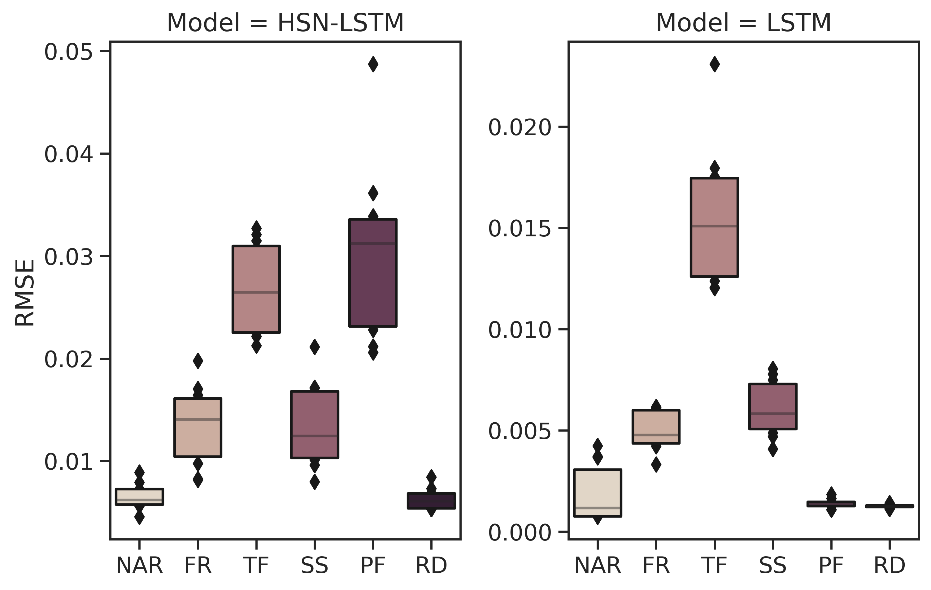
(a) MG. Horizon = 17

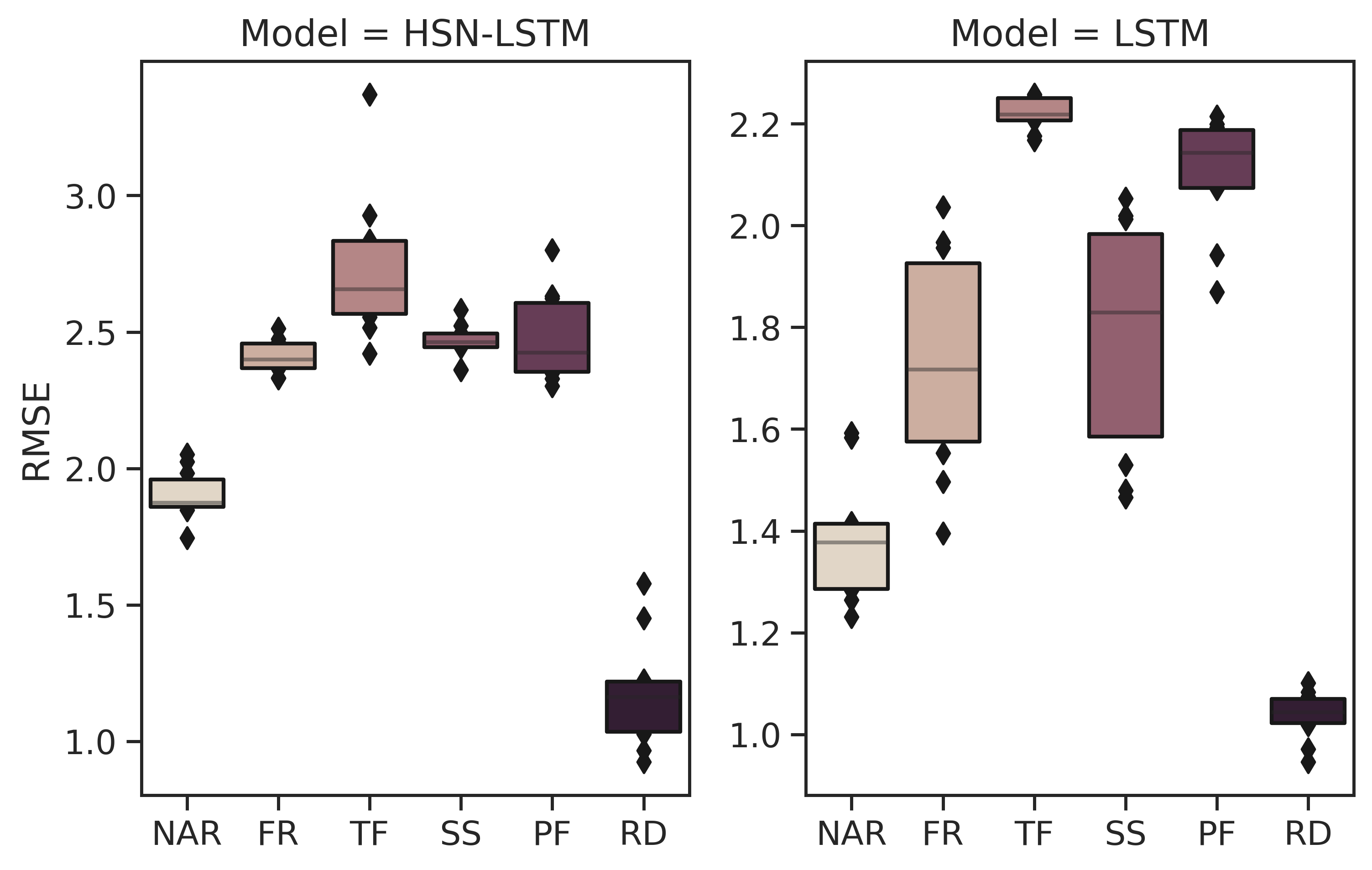
(b) SML. Horizon = 48

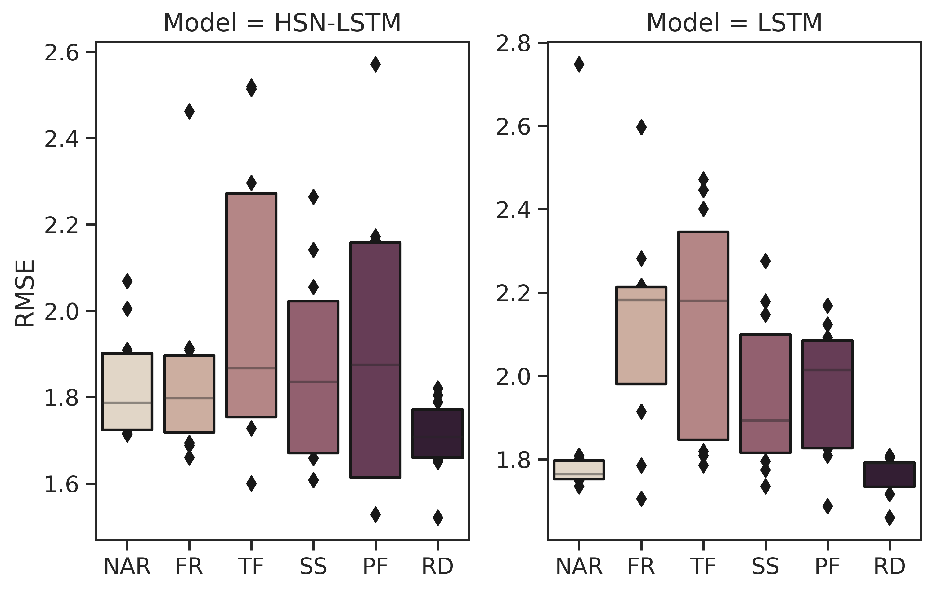
(c) ETTh. Horizon = 48

Figure 4: Boxplots of different training approaches based on the actual RMSE from 10 replicate experiments. The box contains the middle 50% of the data points, which extends from the lower quartile (Q1) to the upper quartile (Q3).

TABLE II: Average RMSE, MAPE of Reinforced Decoder and Counterpart Strategies Based on LSTM over Five Datasets

Strategy

LSTM+NAR

LSTM+FR

LSTM+TF

LSTM+SS

LSTM+PF

LSTM+RD

Metric

RMSE

MAPE

RMSE

MAPE

RMSE

MAPE

RMSE

MAPE

RMSE

MAPE

RMSE

MAPE

MG

17

1.82E-03

1.65E-03

5.00E-03

4.60E-03

1.56E-02

1.41E-02

6.10E-03

5.65E-03

1.38E-03

1.23E-03

1.25E-03

1.15E-03

84

2.13E-03

1.95E-03

8.78E-02

8.75E-02

1.99E-01

1.86E-01

1.05E-01

1.06E-01

1.14E-01

9.79E-02

2.55E-03

2.17E-03

SML

48

1.38E+00

5.01E-02

1.73E+00

6.84E-02

2.22E+00

9.37E-02

1.79E+00

7.03E-02

2.10E+00

8.26E-02

1.04E+00

4.21E-02

96

1.61E+00

6.40E-02

2.26E+00

9.52E-02

2.29E+00

9.89E-02

2.26E+00

9.56E-02

2.67E+00

1.16E-01

1.10E+00

4.26E-02

PM

30

3.75E+01

5.28E-01

3.69E+01

5.07E-01

3.68E+01

4.73E-01

3.72E+01

5.09E-01

3.73E+01

5.18E-01

3.59E+01

5.01E-01

60

3.80E+01

5.53E-01

3.95E+01

5.54E-01

4.00E+01

5.37E-01

3.96E+01

5.62E-01

3.96E+01

5.63E-01

3.61E+01

5.20E-01

ILI

4

6.94E-01

1.20E-01

6.71E-01

1.14E-01

6.73E-01

1.12E-01

6.72E-01

1.14E-01

6.75E-01

1.12E-01

6.68E-01

1.13E-01

12

1.07E+00

2.36E-01

1.02E+00

2.21E-01

1.02E+00

2.17E-01

1.03E+00

2.24E-01

1.03E+00

2.03E-01

9.71E-01

1.78E-01

ETTh

24

1.53E+00

1.35E-01

1.56E+00

1.39E-01

1.63E+00

1.48E-01

1.59E+00

1.43E-01

1.68E+00

1.49E-01

1.49E+00

1.32E-01

48

1.87E+00

1.62E-01

2.13E+00

1.90E-01

2.12E+00

1.88E-01

1.95E+00

1.80E-01

1.96E+00

1.84E-01

1.76E+00

1.55E-01

Count

2

0

1

0

1

17

TABLE III: Average RMSE, MAPE of Reinforced Decoder and Counterpart Strategies Based on HSN-LSTM over Five Datasets

Strategy

HSN-LSTM+NAR

HSN-LSTM+FR

HSN-LSTM+TF

HSN-LSTM+SS

HSN-LSTM+PF

HSN-LSTM+RD

Metric

RMSE

MAPE

RMSE

MAPE

RMSE

MAPE

RMSE

MAPE

RMSE

MAPE

RMSE

MAPE

MG

17

6.55E-03

5.66E-03

1.35E-02

1.18E-02

2.68E-02

2.11E-02

1.35E-02

1.13E-02

3.03E-02

2.28E-02

6.30E-03

5.68E-03

84

6.66E-03

5.92E-03

1.71E-02

1.46E-02

6.08E-02

4.43E-02

1.52E-02

1.33E-02

5.15E-02

3.83E-02

6.45E-03

5.70E-03

SML

48

1.90E+00

7.36E-02

2.32E+00

9.89E-02

2.73E+00

1.12E-01

2.35E+00

1.01E-01

2.48E+00

1.01E-01

1.18E+00

5.05E-02

96

2.07E+00

8.61E-02

2.41E+00

1.01E-01

2.74E+00

1.17E-01

2.46E+00

1.02E-01

2.85E+00

1.20E-01

1.57E+00

6.99E-02

PM

30

3.69E+01

5.66E-01

3.88E+01

6.03E-01

3.93E+01

5.45E-01

3.91E+01

5.94E-01

3.88E+01

5.55E-01

3.64E+01

5.63E-01

60

3.94E+01

6.13E-01

4.09E+01

6.61E-01

4.37E+01

6.80E-01

4.08E+01

6.66E-01

4.44E+01

6.49E-01

3.72E+01

5.93E-01

ILI

4

8.31E-01

1.35E-01

8.92E-01

1.57E-01

8.44E-01

1.41E-01

8.66E-01

1.46E-01

8.40E-01

1.42E-01

8.20E-01

1.35E-01

12

9.57E-01

1.68E-01

1.06E+00

1.93E-01

9.86E-01

1.74E-01

1.33E+00

2.50E-01

1.16E+00

2.08E-01

9.55E-01

1.66E-01

ETTh

24

1.49E+00

1.30E-01

1.66E+00

1.46E-01

1.63E+00

1.50E-01

1.62E+00

1.42E-01

1.57E+00

1.42E-01

1.57E+00

1.40E-01

48

1.83E+00

1.62E-01

1.86E+00

1.71E-01

2.00E+00

1.92E-01

1.86E+00

1.69E-01

1.91E+00

1.81E-01

1.70E+00

1.61E-01

Count

4

0

1

0

0

16

V Results and Discussion

V-A Comparison of Prediction performance

The prediction performance of all benchmark models was examined on the five datasets regarding two accuracy measures, i.e., RMSE and MAPE. The averaged results of the S2S models (LSTM and HSN-LSTM) under different strategies are summarized in Table II and Table III, respectively, with the best results highlighted in bold. The results lead to the following conclusions:

• The proposed reinforced decoder outperforms competing training strategies (the win counts are in the last column) for both univariate and multivariate tasks across different prediction horizons. This demonstrates the effectiveness of the proposed strategy in enhancing the prediction capacity of S2S models applied to time series forecasting.

• The non-autoregressive strategy, NAR, exhibits superior performance compared to FR, illustrating the negative impact of error accumulation. It is conceivable that one reason for the superiority of the RD is its ability to rectify inputs with more accurate ones. Additionally, the better performance of RD compared to NAR substantiates the effectiveness of exploiting valuable information from auxiliary models while preserving temporal dependencies in the decoding process [51, 52].

• Despite the popularity of TF in the multi-step-ahead prediction literature [18, 3, 39], its performance does not consistently surpass that of FR due to exposure bias, e.g., on the MG series, SML series, and ETTh series, which is in agreement with [15]. This is another conceivable reason for the superiority of the proposed approach, which mitigates exposure bias through feeding decoder inputs generated from the same mechanism during both the training and extrapolation stages.

• At least one of the SS and PF strategies has better predictive performance than the TF method in most prediction tasks. These two approaches are improvements over TF and aim to alleviate exposure bias [27, 21, 39], demonstrating the negative effect of exposure bias on predictive performance from another perspective.

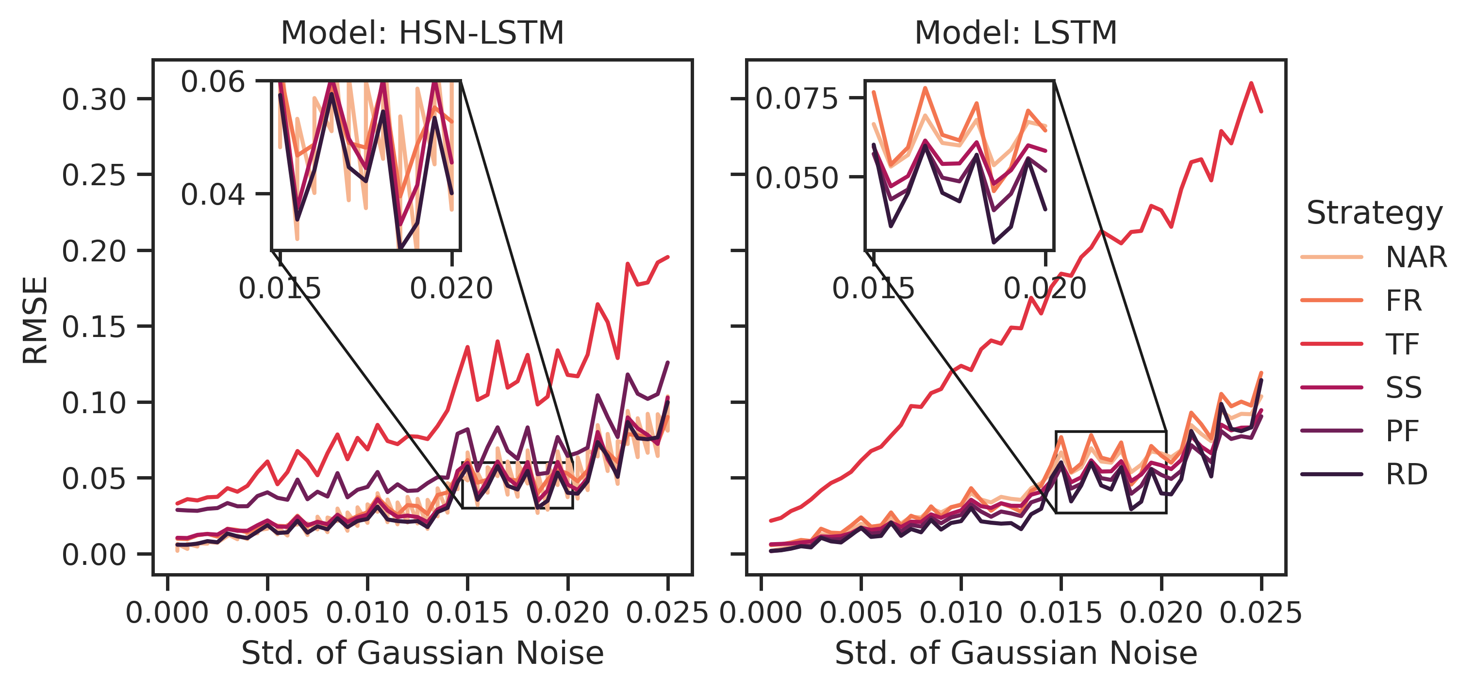
Figure 5: Sensitivity test with different input noise generated by Gaussian function.

In addition, to examine the predictive reliability, the results of 10 repeated experiments are shown as box plots (Fig. 4). Compared with other strategies, the proposed RD strategy not only achieves lower RMSE levels but also has higher prediction stability over repeated trials.

Furthermore, we also conducted input noise experiments on the MG dataset to demonstrate the robustness of the RD strategy [53]. After being trained on noise-free data, the models underwent evaluation using the samples from the test dataset with added noise. The noise was sampled from a Gaussian distribution with the mean equal to 0 and the standard deviation ranging from 1e-4 to 2.5e-3. As shown in Fig. 5, the degradation in model accuracy differs noticeably across training strategies when exposed to noise. Regardless of the underlying S2S model (LSTM or HSN-LSTM), TF exhibits the most pronounced degradation with increasing noise levels, as it uses noise-free true values as input during the training process. The prediction performance of RD remains better than that of the other strategies as the noise level increases. This is due to the mechanism of selecting inputs from a member in the model pool, which implicitly ensembles multiple models. As previous research has demonstrated, ensemble learning can improve the robustness of predictions and enhance generalization ability [2, 28]. Our findings suggest that RD confers advantages in noisy real-world settings due to the introduction of the model pool and adaptive decoder input selection.

V-B Analysis of the Effectiveness of Reinforcement Learning

To further assess the effectiveness of reinforcement learning, the ablation studies of the LSTM-based S2S models were conducted on five datasets. Table IV reports comparative results on the SML series. More results on other datasets are given in Appendix IV.

• AM. This serves as a reference, representing the well-trained auxiliary models (MLP and MSVR).

• LSTM+FR. This S2S model, constructed by LSTM units, always takes self-generated predictions as the decoder inputs without rectification (i.e., trained by FR).

• LSTM+AM. There is no input selection for the decoder. The decoder always takes the predictions from a fixed candidate model (MLP or MSVR) as inputs during both the training and the extrapolation stages.

• LSTM+RD. This is the reinforced decoder approach, where reinforcement learning is used to dynamically select the input-providing model to rectify the decoder inputs.

Compared with LSTM+FR, which relies solely on self-generated predictions, the two LSTM+AM models have better predictive performance, demonstrating the utility of introducing auxiliary models. Moreover, the smaller the prediction error of the auxiliary model, the better the prediction performance of LSTM+AM with its predictions as decoder inputs. This demonstrates that feeding those inputs that are closer to true values helps the decoder reduce error accumulation and improve prediction performance.

In addition, as the prediction performance of the auxiliary models is much better than the results of the decoder itself, LSTM+RD with only one auxiliary model surpasses LSTM+FR and approximates the corresponding LSTM+AM models. This further confirms that the superiority of RD stems from effectively utilizing predictive information from auxiliary models via the REINFORCE method.

TABLE IV: Ablation Study of Reinforce Decoder Base on LSTM over SML Dataset

Model	MLP	MSVR	H = 48 (RMSE)	H = 96 (RMSE)
AM	✓	✗	1.396 ± 8.90E-03	1.461 ± 1.83E-02
	✗	✓	1.551 ± 0.00E+00	1.586 ± 0.00E+00
LSTM+FR	-	-	1.732 ± 2.18E-01	2.259 ± 1.07E-01
LSTM+AM	✓	✗	1.084 ± 7.65E-02	1.146 ± 7.26E-02
	✗	✓	1.109 ± 7.18E-02	1.202 ± 8.84E-02
LSTM+RD	✓	✗	1.085 ± 1.26E-01	1.169 ± 9.85E-03
	✗	✓	1.126 ± 3.85E-02	1.239 ± 9.82E-03
	✓	✓	1.037 ± 4.84E-02	1.096 ± 2.85E-02

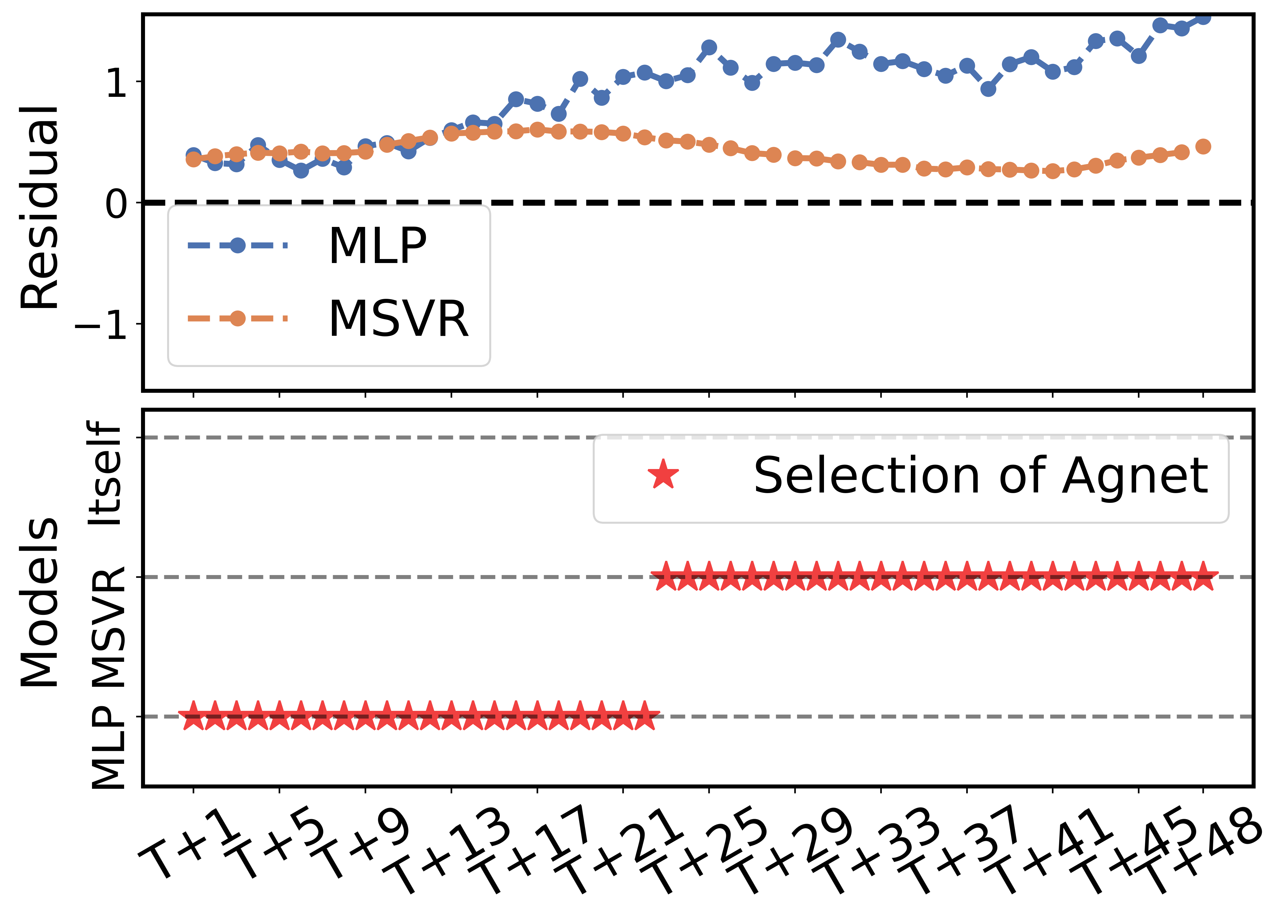
(a) Sample 1

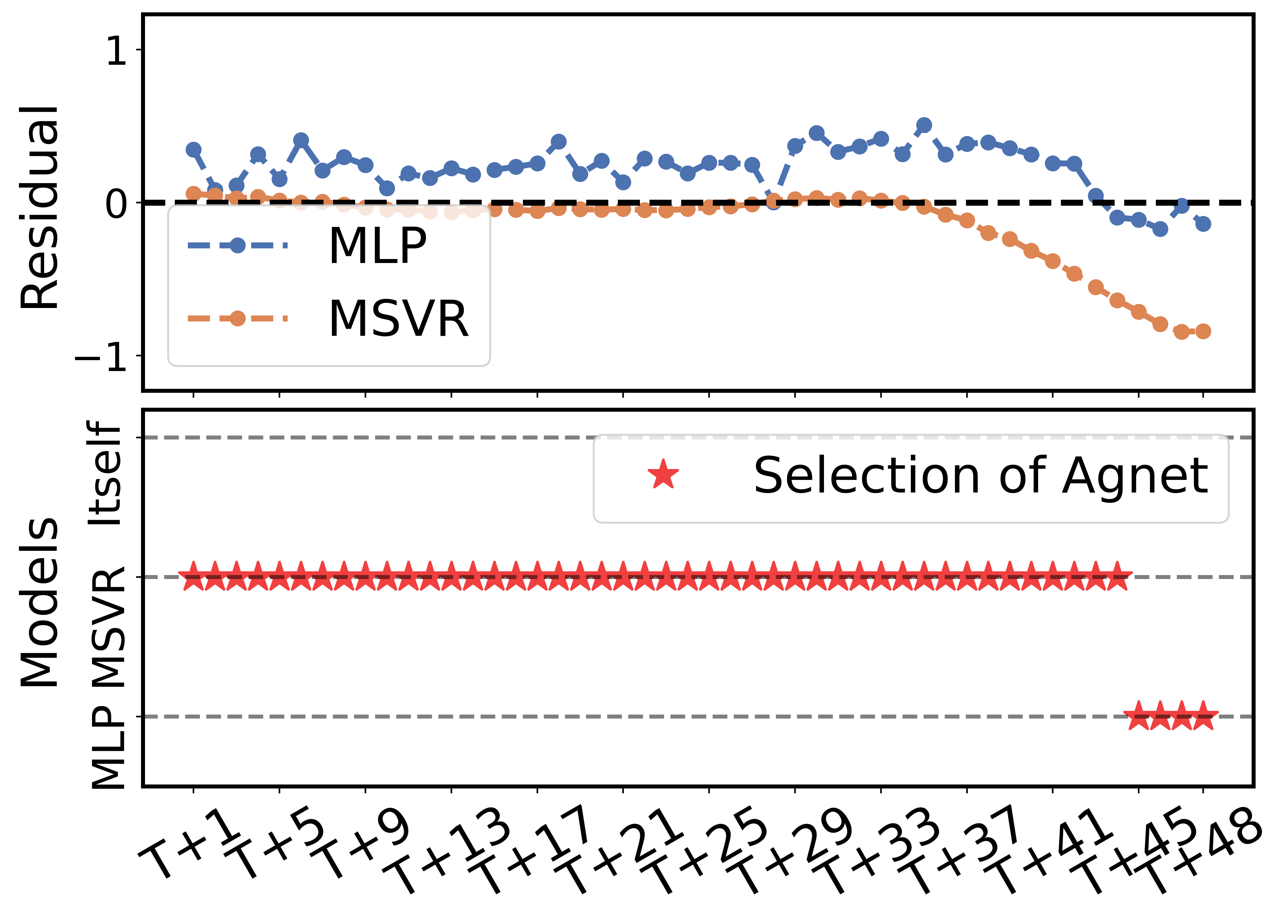
(b) Sample 2

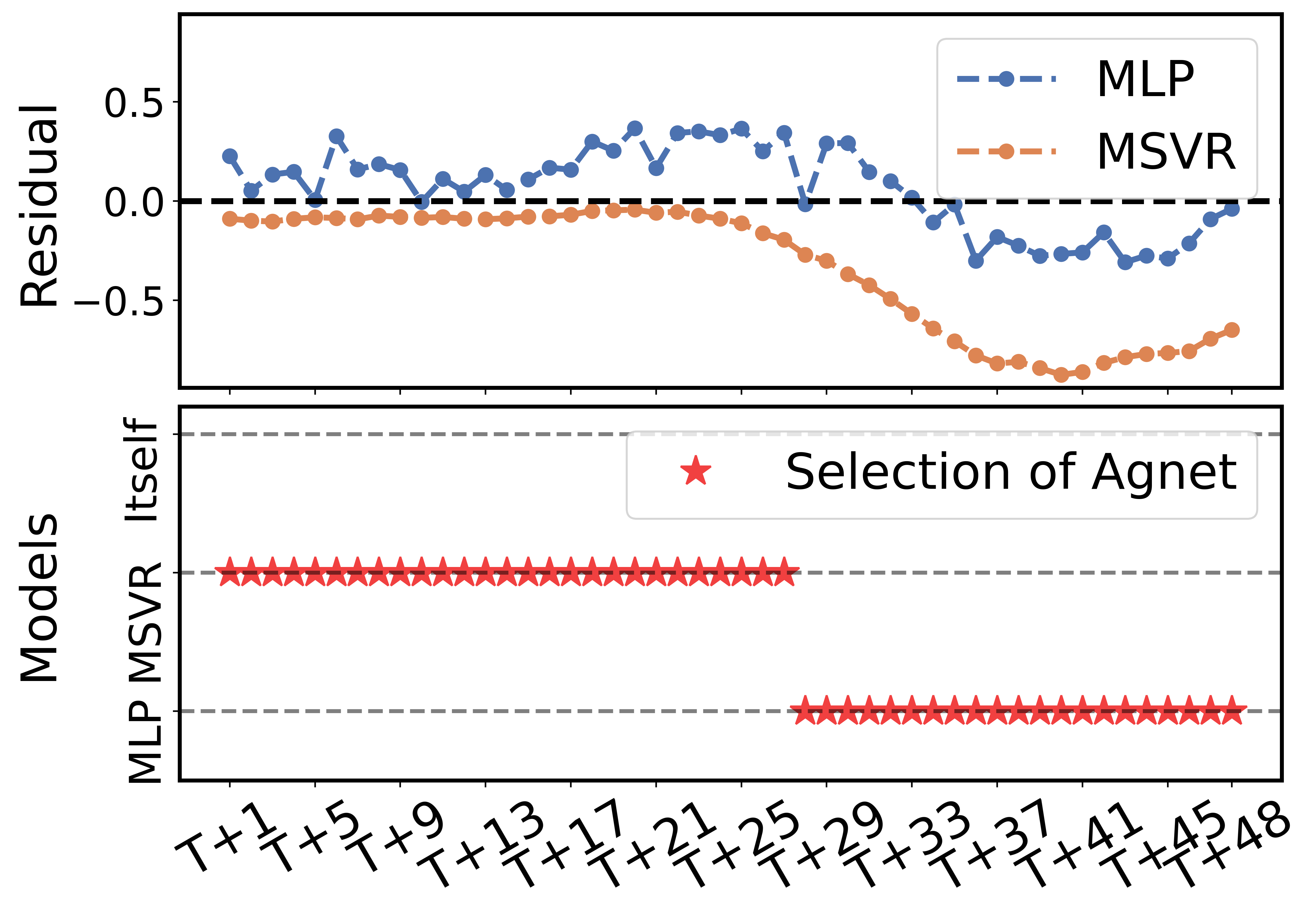
(c) Sample 3

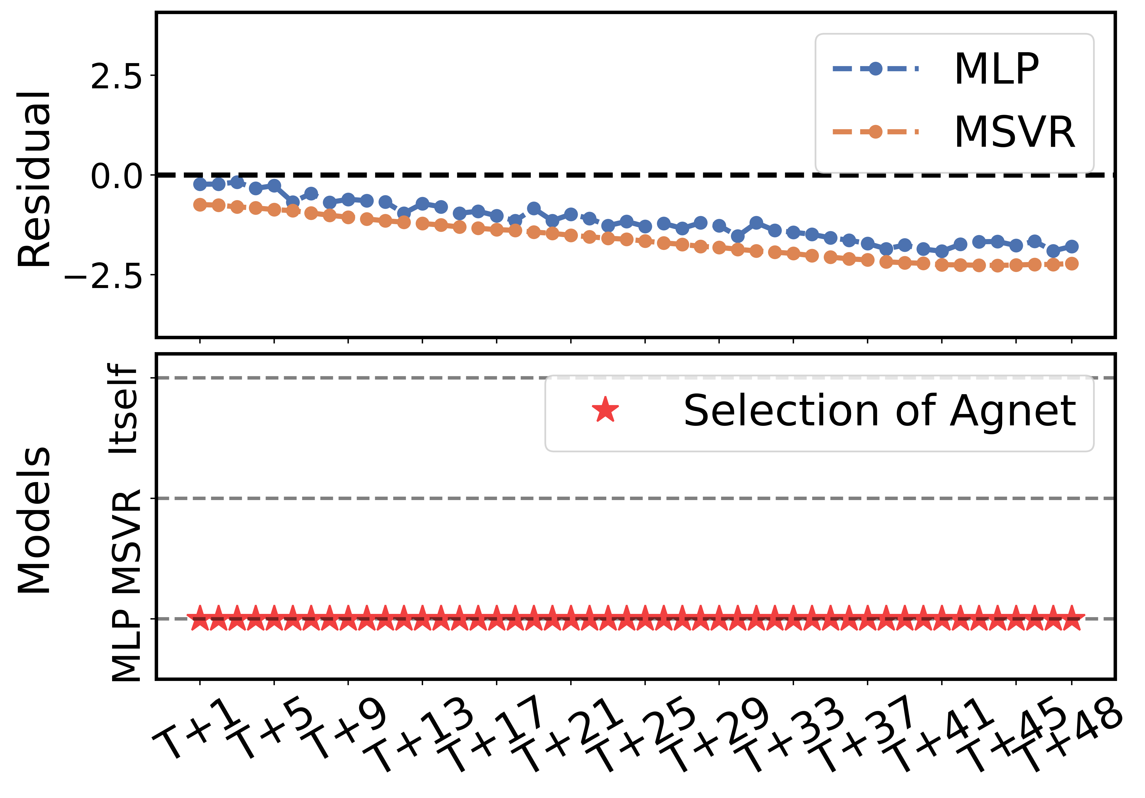
(d) Sample 4

Figure 6: SML-H48: Different samples in testing set. The top half displays the residuals between the true values and the predictions of auxiliary models, while the bottom half shows the actions taken by the agent.

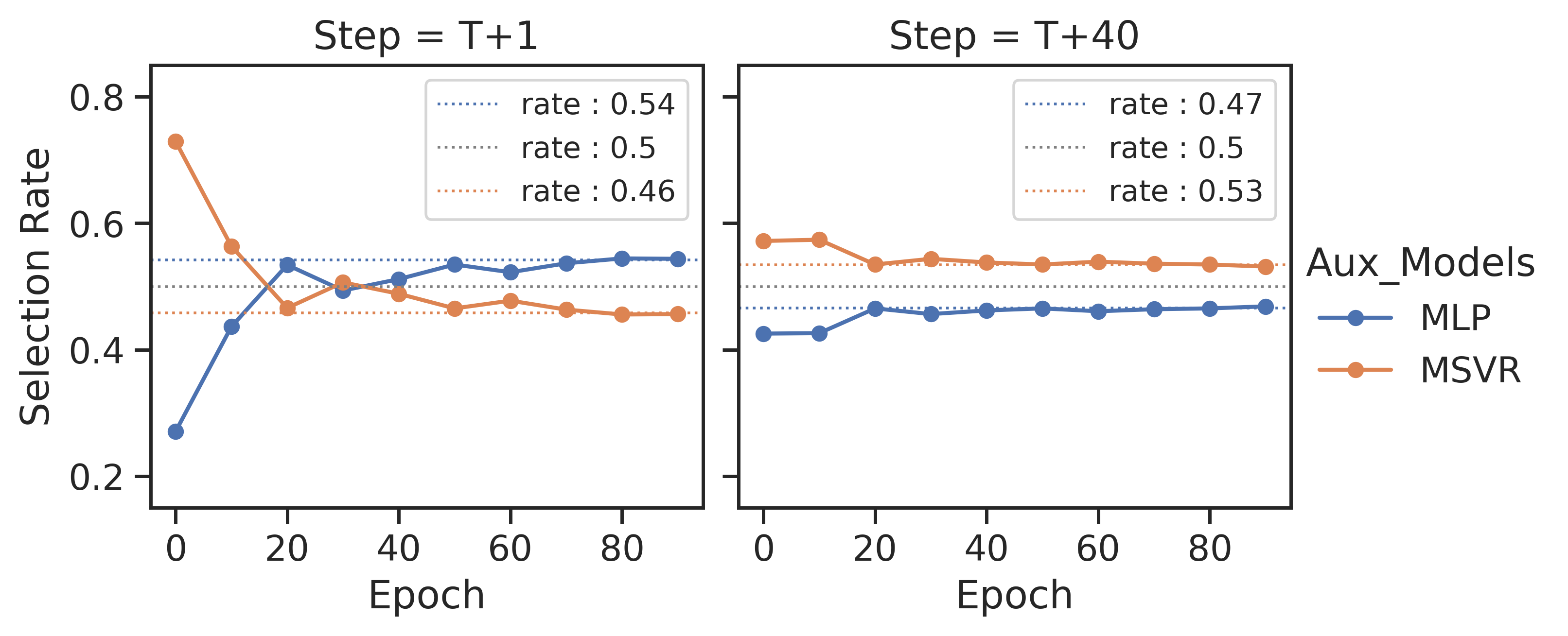
(a) Training set.
At step T + 1, MLP RMSE (0.299) $<$ MSVR RMSE (0.473).
At step T+ 40, MLP RMSE (1.291) $>$ MSVR RMSE (0.723).

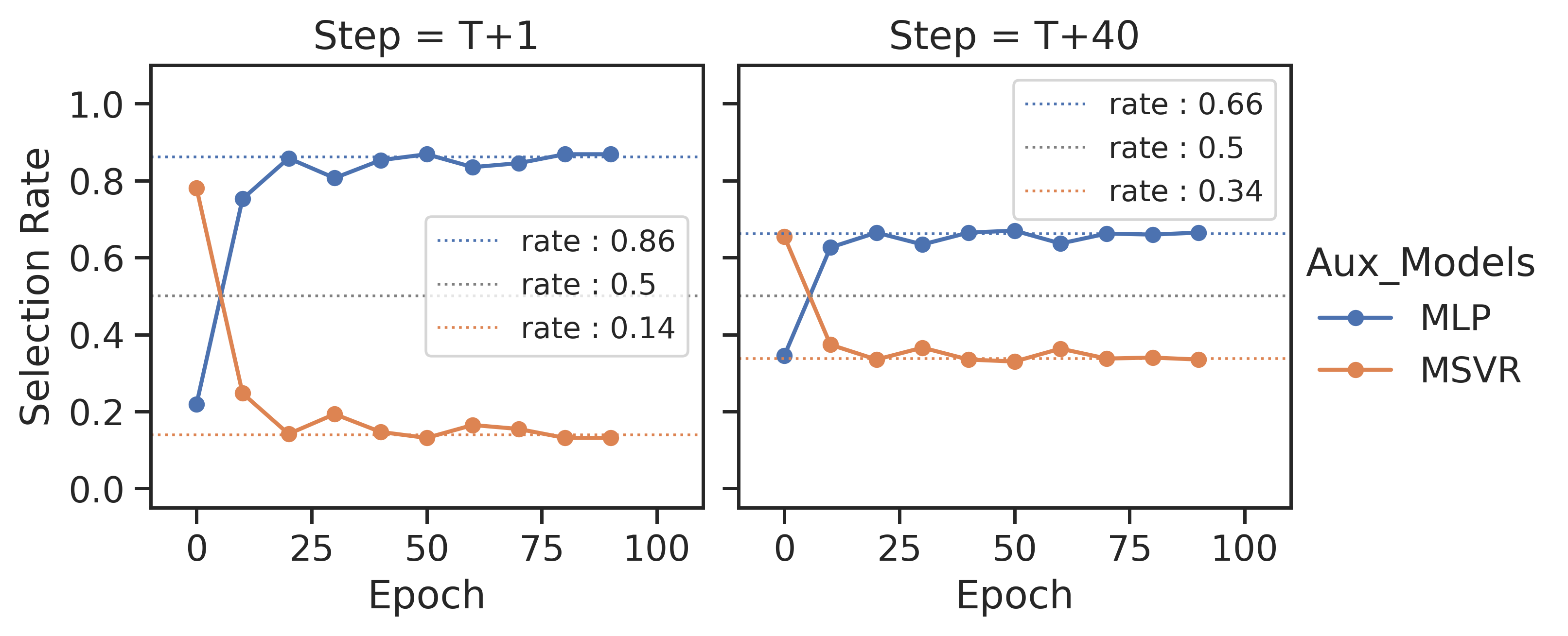
(b) Validation set.
At step T + 1, MLP RMSE (0.392) $<$ MSVR RMSE (0.959).
At step T + 40, MLP RMSE (1.289) $<$ MSVR RMSE (1.406).

Figure 7: SML-H48: The rate of samples in the training and validation sets, where the agent selects the corresponding model.

It is worth noting that although the well-trained MLP outperforms the LSTM+FR and MSVR, LSTM+AM, which directly takes the predictions of the MLP as decoder inputs, fails to achieve the best performance. In contrast, LSTM+RD, which includes the well-trained MLP and MSVR within its model pool, achieves the best results in this task. To gain further insights, we performed slice analysis on the training process of the agent in the LSTM+RD (MSVR, MLP) model when applied to the 48-step-ahead task.

Fig. 7 compares the agent’s actions on the training and validation sets throughout the training process. The samples in the validation set are not involved in updating the agent’s policy. It can be observed that the auxiliary models have differing predictive abilities at different time steps, and the proportion of choices corresponding to the better-performing model significantly increases after training. While MLP has better predictions overall, MSVR excels at certain time steps. This helps to explain why LSTM+RD (MSVR, MLP) outperforms LSTM+AM (MLP). At the same time, it also confirms the need for input selection, as well as the effectiveness of the reinforcement learning method.

In addition, it is noteworthy that, in contrast to its behavior on the training set, the agent chooses the predictions of the well-trained MLP as decoder inputs at time step $T+1$ for 86% of the samples in the validation set. This suggests that the agent is not simply learning to execute a fixed set of actions, but is learning to discern the predictive capabilities of each model for different samples. The insight gleaned from training enables it to select the superior model to provide inputs for the decoder, even in the absence of knowledge regarding actual prediction performances on new samples. This characteristic sets reinforcement learning apart from traditional optimization methods and makes it well-suited with respect to the dynamics inherent in the decoder input selection problem.

Furthermore, we investigated how the dynamic, adaptive features unique to reinforcement learning take effect when rectifying the decoder inputs. Fig. 6 delineates the actions taken by the trained agent at different steps on the test dataset. The results substantiate that, first, different models have varying prediction performances at different time (decoding) steps [28], justifying the necessity of input selection. Second, the input selection scheme developed with reinforcement learning (the trained agent) is not only sample adaptive consistent with the conclusions drawn from Fig. 7, but also adapts to varying decoding steps. This further illustrates the suitability and superiority of reinforcement learning in the context of this problem.

V-C Analysis of the Generalization of Reinforced Decoder on Various S2S Structures

In addition to recurrent neural networks, the S2S models based on the attention mechanism have also recently exhibited promising performance in machine translation and speech recognition [54, 47, 55]. To verify the generality of the RD strategy, we compare it with the above-mentioned strategies (NAR, FR, TF, SS, and PF), based on the well-known self-attention-based model, Informer [47].

TABLE V: Average RMSE, MAPE of Reinforced Decoder and Counterpart Strategies Base on Informer over Five Datasets

Models

Informer+NAR

Informer+FR

Informer+TF

Informer+SS

Informer+PF

Informer+RD

Metric

RMSE

MAPE

RMSE

MAPE

RMSE

MAPE

RMSE

MAPE

RMSE

MAPE

RMSE

MAPE

MG

17

1.44E-02

1.33E-02

2.19E-02

1.88E-02

3.35E-02

3.06E-02

2.19E-02

1.96E-02

1.54E-01

1.51E-01

1.40E-02

1.20E-02

84

2.48E-02

2.23E-02

4.16E-02

3.79E-02

1.74E-01

1.38E-01

4.47E-02

4.10E-02

2.47E-01

2.49E-01

2.65E-02

2.35E-02

SML

48

2.44E+00

1.02E-01

2.51E+00

1.03E-01

2.52E+00

1.08E-01

2.48E+00

1.04E-01

2.82E+00

1.26E-01

2.34E+00

9.49E-02

96

2.46E+00

1.09E-01

2.87E+00

1.27E-01

3.01E+00

1.37E-01

2.51E+00

1.03E-01

3.90E+00

1.78E-01

2.42E+00

1.07E-01

PM

30

3.97E+01

6.15E-01

3.99E+01

6.26E-01

3.96E+01

5.27E-01

3.92E+01

6.51E-01

4.23E+01

5.96E-01

3.92E+01

6.04E-01

60

4.03E+01

6.48E-01

4.11E+01

6.46E-01

4.15E+01

5.70E-01

4.08E+01

6.87E-01

4.50E+01

6.68E-01

4.02E+01

6.49E-01

ILI

4

1.00E+00

1.48E-01

9.52E-01

1.56E-01

9.12E-01

1.49E-01

8.99E-01

1.39E-01

9.42E-01

1.46E-01

8.53E-01

1.28E-01

12

1.02E+00

1.50E-01

1.08E+00

1.49E-01

9.85E-01

1.54E-01

1.05E+00

1.51E-01

1.10E+00

2.04E-01

9.48E-01

1.57E-01

ETTh

24

2.09E+00

1.87E-01

2.01E+00

1.82E-01

1.83E+00

1.67E-01

2.03E+00

1.86E-01

2.40E+00

2.18E-01

1.72E+00

1.58E-01

48

2.27E+00

1.99E-01

2.46E+00

2.17E-01

2.03E+00

1.88E-01

2.04E+00

1.83E-01

3.26E+00

2.86E-01

1.79E+00

1.59E-01

Count

1

1

2

2

1

14

In particular, Informer (+NAR) predicts outputs by one forward procedure, i.e., generative inference, rather than auto-regressive decoding. For the Informer+RD model, the environment states observed by the agent are defined as the outputs generated by the self-attention modules within the decoder. These outputs serve as the contextual information that the agent uses to make decisions regarding input selection during the dynamic decoding process. The hyperparameters of Informer followed [47] to ensure a fair comparison and the details are provided in Appendix III. Table V reports the results, with the smallest value highlighted in bold. The results show that the RD strategy still achieves the best performance among various training strategies, demonstrating its architecture-agnostic utility for optimizing S2S models.

As Informer is well-suited to long-range dependencies, we further examined the NAR, FR, and RD strategies on the ETTh dataset with longer prediction horizons (Fig. 8). Overall, the prediction performance of the FR strategy decreases rapidly as the forecasting horizon increases due to the accumulation of errors. In contrast, RD mitigates this by rectifying decoder inputs through the introduction of multiple auxiliary models and adaptive selection (by the agent), sustaining strong performance even for longer horizons. Furthermore, RD also outperforms the NAR strategy thanks to external valuable information from auxiliary models.

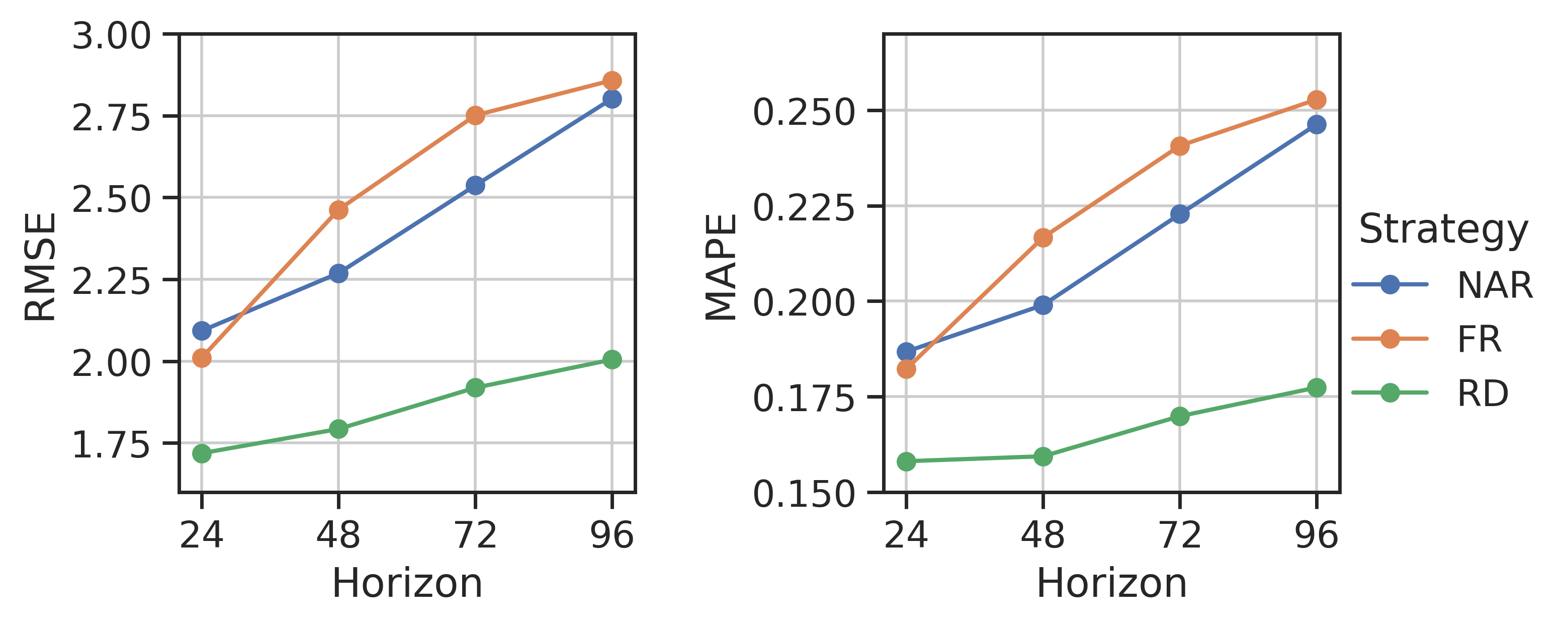
Figure 8: Comparison of evaluation metric curves of Informer+NAR, Informer+FR, and Informer+RD for different horizons on ETTh dataset.

VI Conclusion

The sequence-to-sequence (S2S) models based on recurrent neural networks (RNNs) have been widely applied to multi-step-ahead time series prediction tasks. However, common training approaches, such as free running and teacher forcing, rely exclusively on self-generated predictions or true values, and, thus, suffer from rapid error amplification and exposure bias, respectively. To address these problems, this study proposed a novel training and decoding strategy called reinforced decoder (RD), which introduces a model pool to provide inputs for the decoder and exploits reinforcement learning (RL) to dynamically select the optimal input-providing model.

Through an extensive set of simulated and real-world dataset experiments, we demonstrate the superior performance of RD strategy in enhancing the prediction accuracy of RNN-based S2S models. Our approach achieves improved results compared to conventional training methods, such as free running and teacher forcing, as well as recent successful approaches including professor forcing [21] and schedule sampling [27]. Moreover, the RNN-based S2S models with RD strategy also outperform those with non-autoregressive decoding structures, such as dense layer [10, 17] and attention-based schemes [16]. We find that the performance gains come from the rectification of decoder inputs by introducing auxiliary models, with reinforcement learning enabling an adaptive and efficient mechanism for input selection. Additionally, when applying our method to the self-attention-based S2S model, i.e., Informer [47], the reinforced decoder continues to exhibit promising forecasting ability. As the experimental results and our analysis indicate, the proposed approach provides a general and powerful training and decoding means for constructing S2S models applied in multi-step-ahead time series prediction tasks.

For future works, we will also investigate the possibility of applying the RL module to other multi-step-ahead time series forecasting models based on the auto-regressive mechanism.

References

- [1] K. Zhang, H. Cao, J. Thé, and H. Yu, “A hybrid model for multi-step coal price forecasting using decomposition technique and deep learning algorithms,” Appl. Energy, vol. 306, p. 118011, 2022.
- [2] C. Chen and H. Liu, “Dynamic ensemble wind speed prediction model based on hybrid deep reinforcement learning,” Adv. Eng. Inf., vol. 48, 2021.
- [3] Y. Wang, T. Chen, S. Zhou, F. Zhang, R. Zou, and Q. Hu, “An improved wavenet network for multi-step-ahead wind energy forecasting,” Energ. Convers. Manage., vol. 278, p. 116709, Feb. 2023.
- [4] J. Han, H. Liu, H. Zhu, and H. Xiong, “Kill two birds with one stone: A multi-view multi-adversarial learning approach for joint air quality and weather prediction,” IEEE Trans. Knowl. Data Eng., vol. 35, no. 11, pp. 11 515–11 528, 2023.
- [5] Z. Xiang, J. Yan, and I. Demir, “A rainfall-runoff model with LSTM-based sequence-to-sequence learning,” Water Resour. Res., vol. 56, no. 1, 2020.
- [6] K. Kumar and V. K. Jain, “Autoregressive integrated moving averages (ARIMA) modelling of a traffic noise time series,” Appl. Acoust., vol. 58, no. 3, pp. 283–294, 1999.
- [7] S. V. Dudul, “Prediction of a lorenz chaotic attractor using two-layer perceptron neural network,” Appl. Soft Comput., vol. 5, no. 4, pp. 333–355, 2005.
- [8] Tuia, D., Verrelst, J., Alonso, L., Perez-Cruz, F., Camps-Valls, and G., “Multioutput support vector regression for remote sensing biophysical parameter estimation,” IEEE Geosci. Remote Sens. Lett., 2011.
- [9] L. Breiman, “Random Forests,” Mach. Learn., vol. 45, no. 1, pp. 5–32, Oct. 2001.
- [10] H. Hewamalage, C. Bergmeir, and K. Bandara, “Recurrent neural networks for time series forecasting: Current status and future directions,” Int. J. Forecasting, vol. 37, no. 1, pp. 388–427, 2021.
- [11] Z. Yang, W. Yan, X. Huang, and L. Mei, “Adaptive temporal-frequency network for time-series forecasting,” IEEE Trans. Knowl. Data Eng., vol. 34, no. 4, pp. 1576–1587, 2022.
- [12] F. Ilhan, O. Karaahmetoglu, I. Balaban, and S. S. Kozat, “Markovian RNN: An adaptive time series prediction network with HMM-based switching for nonstationary environments,” IEEE Trans. Neural Netw. Learn. Syst., vol. 34, no. 2, pp. 715–728, Feb. 2023.
- [13] D. Salinas, V. Flunkert, J. Gasthaus, and T. Januschowski, “DeepAR: Probabilistic forecasting with autoregressive recurrent networks,” Int. J. Forecasting, vol. 36, no. 3, pp. 1181–1191, 2020.
- [14] Z. Zheng and Z. Zhang, “A stochastic recurrent encoder decoder network for multistep probabilistic wind power predictions,” IEEE Trans. Neural Netw. Learn. Syst., early access, jan 2023.
- [15] M. Sangiorgio, F. Dercole, and G. Guariso, “Forecasting of noisy chaotic systems with deep neural networks,” Chaos. Soliton. Fract., vol. 153, p. 111570, Dec. 2021.
- [16] W. Zheng, P. Zhao, G. Chen, H. Zhou, and Y. Tian, “A hybrid spiking neurons embedded lstm network for multivariate time series learning under concept-drift environment,” IEEE Trans. Knowl. Data Eng., vol. 35, no. 7, pp. 6561–6574, 2023.
- [17] R. Wen, K. Torkkola, B. M. Narayanaswamy, and D. Madeka, “A multi-horizon quantile recurrent forecaster,” in Proc. Adv. Neural Inf. Process. Syst., 2017.
- [18] R. J. Williams and D. Zipser, “A learning algorithm for continually running fully recurrent neural networks,” Neural Comput., vol. 1, no. 2, pp. 270–280, 1989.
- [19] M. Ranzato, S. Chopra, M. Auli, and W. Zaremba, “Sequence level training with recurrent neural networks,” in Proc. Int. Conf. Learn. Represent., 2016.
- [20] M. Sangiorgio and F. Dercole, “Robustness of lstm neural networks for multi-step forecasting of chaotic time series,” Chaos. Soliton. Fract., vol. 139, p. 110045, Oct. 2020.
- [21] A. Goyal, A. Lamb, Y. Zhang, S. Zhang, A. Courville, and Y. Bengio, “Professor forcing: A new algorithm for training recurrent networks,” in Proc. Adv. Neural Inf. Proces. Syst., 2016.
- [22] J. Li, W. Monroe, T. Shi, S. Jean, A. Ritter, and D. Jurafsky, “Adversarial learning for neural dialogue generation,” in Proc. Adv. Neural Inf. Proces. Syst., Sep. 2017, pp. 2157–2169.
- [23] J. Guo, S. Lu, H. Cai, W. Zhang, Y. Yu, and J. Wang, “Long text generation via adversarial training with leaked information,” in Proc. AAAI Conf. Artif. Intell., Feb. 2018, pp. 5141–5148.
- [24] T. Salimans, I. J. Goodfellow, W. Zaremba, V. Cheung, A. Radford, and X. Chen, “Improved techniques for training gans,” in Proc. Adv. Neural Inf. Process. Syst., 2016, pp. 2226–2234.
- [25] L. Metz, B. Poole, D. Pfau, and J. Sohl-Dickstein, “Unrolled generative adversarial networks,” in Proc. Int. Conf. Mach. Learn., 2017.
- [26] Y. Taigman, L. Wolf, A. Polyak, and E. Nachmani, “Voiceloop: Voice fitting and synthesis via a phonological loop,” in Proc. Int. Conf. Mach. Learn., 2018.
- [27] S. Bengio, O. Vinyals, N. Jaitly, and N. Shazeer, “Scheduled sampling for sequence prediction with recurrent neural networks,” in Proc. Adv. Neural Inf. Proces. Syst., 2015, pp. 1171–1179.
- [28] Y. Fu, D. Wu, and B. Boulet, “Reinforcement learning based dynamic model combination for time series forecasting,” in Proc. AAAI Conf. Artif. Intell., 2022, pp. 6639–6647.
- [29] R. J. Williams, “Simple statistical gradient-following algorithms for connectionist reinforcement learning,” Mach. Learn., vol. 8, no. 3-4, pp. 229–256, 1992.
- [30] T. K. Das, A. Gosavi, S. Mahadevan, and N. Marchalleck, “Solving semi-markov decision problems using average reward reinforcement learning,” Manage. Sci., vol. 45, no. 4, pp. 560–574, 1999.
- [31] G. Manganini, M. Pirotta, M. Restelli, L. Piroddi, and M. Prandini, “Policy search for the optimal control of markov decision processes: A novel particle-based iterative scheme,” IEEE Trans. Cybern., vol. 46, no. 11, pp. 2643–2655, Nov. 2016.
- [32] X. Wang, S. Wang, X. Liang, D. Zhao, J. Huang, X. Xu, B. Dai, and Q. Miao, “Deep reinforcement learning: A survey,” IEEE Trans. Neural Netw. Learn. Syst., pp. 1–15, 2022.
- [33] I. Sutskever, O. Vinyals, and Q. V. Le, “Sequence to sequence learning with neural networks,” in Proc. Adv. Neural Inf. Process. Syst., Dec. 2014.
- [34] J. L. Elman, “Finding structure in time,” Cognit. Sci., vol. 14, no. 2, pp. 179–211, 1990.
- [35] S. Hochreiter and J. Schmidhuber, “Long short-term memory,” Neural Comput., vol. 9, no. 8, pp. 1735–1780, 1997.
- [36] K. Cho, B. Van Merrienboer, C. Gulcehre, D. Bahdanau, F. Bougares, H. Schwenk, and Y. Bengio, “Learning phrase representations using RNN encoder-decoder for statistical machine translation,” in Proc. Conf. Empir. Methods Nat. Lang. Process., 2014, pp. 1724–1734.
- [37] I. Goodfellow, Y. Bengio, and A. Courville, Deep Learning. MIT Press, 2016, http://www.deeplearningbook.org.
- [38] P. Werbos, “Backpropagation through time: What it does and how to do it,” Proc. IEEE, vol. 78, no. 10, pp. 1550–1560, 1990.
- [39] R. Bolboacă and P. Haller, “Performance analysis of long short-term memory predictive neural networks on time series data,” Mathematics, vol. 11, no. 6, p. 1432, 2023.
- [40] J. P. Hanna and P. Stone, “Reducing sampling error in policy gradient learning,” in Proc. Int. Conf. Auton. Agents Multiagent Syst., 2019, pp. 1016–1024.
- [41] Y. Bao, T. Xiong, and Z. Hu, “Multi-step-ahead time series prediction using multiple-output support vector regression,” Neurocomputing, vol. 129, pp. 482–493, 2014.
- [42] S. Yang and Y. Bao, “Comprehensive learning particle swarm optimization enabled modeling framework for multi-step-ahead influenza prediction,” Appl. Soft Comput., vol. 113, 2021.
- [43] F. T. S, Mathematical Statistics: A Decision Theoretic Approach. New York, NY: Academic Press, 1967.
- [44] M. Srouji, J. Zhang, and R. Salakhutdinov, “Structured control nets for deep reinforcement learning,” in Proc. Int. Conf. Mach. Learn., 2018, pp. 4749–4758.
- [45] R. S. Sutton and A. G. Barto, “Reinforcement learning: An introduction,” IEEE Trans. Neural Networks, vol. 9, no. 5, pp. 1054–1054, 1998.
- [46] F. Zamora-Martínez, P. Romeu, P. Botella-Rocamora, and J. Pardo, “On-line learning of indoor temperature forecasting models towards energy efficiency,” Energy Build., vol. 83, pp. 162–172, Nov. 2014.
- [47] H. Zhou, S. Zhang, J. Peng, S. Zhang, J. Li, H. Xiong, and W. Zhang, “Informer: Beyond efficient transformer for long sequence time-series forecasting,” in Proc. AAAI Conf. Artif. Intell., 2021.
- [48] X. Zhang, K. He, and Y. Bao, “Error-feedback stochastic modeling strategy for time series forecasting with convolutional neural networks,” Neurocomputing, vol. 459, pp. 234–248, 2021.
- [49] N. Muralidhar, S. Muthiah, K. Nakayama, R. Sharma, and N. Ramakrishnan, “Multivariate long-term state forecasting in cyber-physical systems: A sequence to sequence approach,” in Proc. IEEE Int. Conf. Big Data, 2019, pp. 543–552.
- [50] J. Bergstra and Y. Bengio, “Random search for hyper-parameter optimization,” J. Mach. Learn. Res., vol. 13, no. 1, pp. 281–305, 2012.
- [51] M. Marcellino, J. H. Stock, and M. W. Watson, “A comparison of direct and iterated multistep AR methods for forecasting macroeconomic time series,” J. Econometrics, vol. 135, no. 1, pp. 499–526, 2006.
- [52] M. G. De Giorgi, M. Malvoni, and P. M. Congedo, “Comparison of strategies for multi-step ahead photovoltaic power forecasting models based on hybrid group method of data handling networks and least square support vector machine,” Energy, vol. 107, pp. 360–373, 2016.
- [53] X. Zhang, C. Zhong, J. Zhang, T. Wang, and W. W. Y. Ng, “Robust recurrent neural networks for time series forecasting,” Neurocomputing, vol. 526, pp. 143–157, Mar. 2023.
- [54] K. Yao, L. Zhang, D. Du, T. Luo, L. Tao, and Y. Wu, “Dual encoding for abstractive text summarization,” IEEE Trans. Cybern., vol. 50, no. 3, pp. 985–996, 2020.
- [55] H. Wu, J. Xu, J. Wang, and M. Long, “Autoformer: Decomposition transformers with auto-correlation for long-term series forecasting,” in Proc. Adv. Neural Inf. Proces. Syst., 2021.