Optimal Convex Cover as Collision-free Space Approximation for Trajectory Generation

Abstract

We propose an online iterative algorithm to find a suitable convex cover to under-approximate the free space for autonomous navigation to delineate Safe Flight Corridors (SFC). The convex cover consists of a set of polytopes such that the union of the polytopes represents obstacle-free space, allowing us to find trajectories for robots that lie within the convex cover. In order to find the SFC that facilitates optimal trajectory generation, we iteratively find overlapping polytopes of maximum volumes that include specified waypoints initialized by a geometric or kinematic planner. Constraints at waypoints appear in two alternating stages of a joint optimization problem, which is solved by a method inspired by the Alternating Direction Method of Multipliers (ADMM) with partially distributed variables. We validate the effectiveness of our proposed algorithm using a range of parameterized environments and show its applications for two-stage motion planning.

1 Introduction

All motion and path planning algorithms require the representation of the environment for collision avoidance and checking. Different algorithms choose different representations. Exact methods map obstacles from the workspace into the configuration space, this gives guarantees of completeness and optimality but may be computationally intractable [1]. Sampling-based methods do not need to represent the environment explicitly but they only offer probabilistic guarantees and may still require an excessively large number of samples in cluttered high-dimensional spaces [2]. A middle ground has become popular over the past few years, including convex approximation of the collision-free space. This is computationally attractive because it allows us to convert motion planning into an efficient optimization problem. This problem is also tractable because collision-free space can be described by a set of linear constraints corresponding to each of the polytopes in the cover.

Figure 1: The influence of convex cover on trajectory generation. (a) Seed points (blue) determine the volume of the largest polytope (red) within a map (obstacles in grey). The largest-volume polytope can be identified by selecting the seed point at the orange star. (b) Polytopes may not always cover a large part of the trajectory, even if they have a large volume. (c, d) Given an initial path (black), the quality of the final trajectory (green) depends strongly upon which convex cover was used to optimize it.

One of the key issues in this approach pertains to computing a good approximation of the environment. One could find a convex cover by a collection of convex sets such that the union of the convex sets can cover a given region or include a given guess for a trajectory. Solving the subproblem of extracting a single convex decomposition from a seed point or convex body is usually involved in generating the convex cover [3, 4, 5, 6, 7]. Considering the example in Fig. 1(a), an ideal single convex decomposition should capture most of the free space. There should also be enough overlaps between different polytopes (ellipsoids are another popular choice) in the convex cover, at least successive polytopes as a “Safe Flight Corridor” (SFC). The properties of the SFC will influence the ultimate geometric feasible region for optimization. Many existing approaches generate an SFC by selecting seed points around the initial path [8, 9, 10]. However, such covers are not ideal in practice because the selection of SFC is greedy and does not account for trajectory planning. It is difficult to determine how the geometric shapes and volumes of the polytopes interplay with the dynamical feasibility and optimality of the trajectories computed by the lower-level optimization procedure. Fig. 1(b)-(d) shows some examples of potential factors like polytope volumes and overlapping areas that potentially change the final cover of a trajectory. As a consequence, existing methods cannot give any guarantees on the quality of the SFC or the trajectory. This suggests that coupled program: front-end path planning, free space approximation using a convex cover, and trajectory generation within this cover, cannot be solved independently.

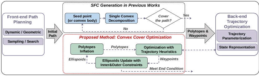
Figure 2: SFC generation pipeline in two-stage planning modules of previous works and our method. In the proposed method, we jointly optimize the path represented by waypoints together with polytopes and ellipsoids that form a convex cover of the path in free space to generate a better back-end trajectory downstream.

To address optimal SFC generation, we introduce a novel algorithm that optimizes the convex cover of the environment to aid in trajectory planning for quadrotors (and other mobile robots with dynamic constraints). It updates the polytopes that form the convex cover and maximizes the volumes of ellipsoids inscribed within these polytopes given the waypoints updated by using heuristic functions to approximate trajectory cost. These include two alternating stages of a joint optimization problem, which is solved by a method inspired by the Alternating Direction Method of Multipliers (ADMM) [11] with partially distributed variables. The pipeline is shown in Fig. 2 in comparison to previous works. This approach is validated using a large variety of synthetic environments to demonstrate its flexibility and robustness.

Contributions: (1) We formulate an SFC generation problem to identify the optimal convex cover in collision-free space for trajectory optimization. (2) We design a novel iterative algorithm based on the distributed ADMM for computational efficiency. (3) We extensively evaluate our method, benchmark it in environments with varying complexities, and present the first thorough analysis of the influence of the front-end plan path and SFC on the trajectory cost.

2 Related works

In real-world representations of geometric environments, obstacles or objects can be decomposed into a series of convex shapes to assist obstacle avoidance strategies. There are traditional methods to solve exact and approximate convex decomposition [12, 13, 14] or neural networks to learn the convex primitives [15]. However, decomposing obstacles would result in a large number of small pieces that can lead to significant computational costs. Instead, extracting the convex representation of nonconvex free space is more efficient for motion planning problem formulation [16, 17, 10, 18, 19, 20, 21]. Collision-free corridors or graphs can be generated using boxes[16, 17], sphere or ellipsoids[19, 18] and polytopes[10, 20] within environments represented by noisy point clouds or obstacle maps. A more detailed reviews of free-space decomposition are listed as follows:

Single Convex Decomposition of Free Space. To extract convex regions from nonconvex environments, [3] proposed an algorithm of Iterative Regional Inflation by Semidefinite Programming (IRIS) to generate maximum volume polytopes around convex obstacles given a seed point. The iterative optimization process involved sequentially quadratic programming to find separating hyperplanes toward obstacles, followed by semidefinite programming to determine the maximum-volume ellipsoid (inner Löwner-John Ellipsoid [22]) within this polytope. However, considering the expensive computation of this approach, more works focused on improving the efficiency of the process, such as generating polytopes on line segments [8], or convex bodies [7]. With given voxel maps as inputs, [21] proposed parallel convex inflation of axis-aligned cubes on axis directions by checking the voxel points incrementally, which can achieve resolution near real-time. Moreover, in [23], the authors introduced a stereographic projection technique to project obstacle points or point clouds and convert them into a convex hull. The generative region is over-conservative for application, which is improved by [6] using sphere flipping to generate star-convex shapes and further refined into convex.

Convex Cover of a Global Map. While previous works exist for inflating a single convex region within naturally nonconvex environments, determining an optimal cover of local or entire free space remains challenging. The performance of IRIS-based decomposition for global convex covers relies heavily on the distribution of seed points, which is manually set in [3, 24]. To improve the sampling efficiency, the work [5] leveraged the topology property of the objects and employed skeleton structures to position convex primitives. Rejection sampling methods are utilized in [18, 10] to refine seed point selection outside existing polytopes or ellipsoids until the desired environment coverage is achieved. Furthermore, [20] iteratively conducted sampling to update clique covers of visibility graphs and inflate polytopes. With the convex free-space maps, the trajectory generation problem can be addressed by decoupled [10] or joint optimization [24, 25].

Convex Cover along a Trajectory. For real-world deployments, computation efficiency is more important and is usually achieved by narrowing the solution space of trajectory optimization. A two-stage planning framework, involving front-end path planning with geometric constraints followed by back-end optimization within the same homotopy class, has been extensively discussed in [26] and applied to various environments decomposed by SFC. The authors in [8] proposed a jump point search (JPS) to find a geometric path composed of line segments and initialize ellipsoids on lines with one iteration polytope inflation. For general polytopes generation using seed points or lines, different paths from front-end pathfinding can be applied by iteratively checking the farthest point along the path within the polytope as the next sample points [9, 10]. However, the above methods either choose line segments or employ a greedy approach to find the next waypoint as seeds, potentially resulting in suboptimal trajectories, particularly in narrow hallways. Our approach lies within this category and focuses on decomposing collision-free space to SFC. This involves factors such as convex approximation accuracy, division of trajectory segments, and ensuring connectivity of convex regions between waypoints.

3 Problem Statement

3.1 Trajectory Optimization Formulation

We consider the problem of finding an optimal trajectory for a $s-$order integrator system, represented by states $x(t)$ and control inputs $u(t)$, with traversal time $T$ that passes through collision-free space $\mathcal{F}_{free}$. Given a start state $x_{0}\in\mathcal{F}_{free}$ and a feasible goal region $\mathcal{F}_{goal}\subseteq\mathcal{F}_{free}$, the trajectory optimization problem is formulated as

$$\min_{x(t),T}\ \int_{0}^{T}\|u(t)\|^{2}dt+w_{t}\gamma(T),$$ (1a)

$${\rm s.t.}\ \ x^{(s)}(t)=u(t),\ \forall t\in[0,T],$$ (1b)

$$\qquad x(0)=x_{0},\ \ x(T)\in\mathcal{F}_{goal},$$ (1c)

$$\qquad x(t)\in\mathcal{F}_{free},\ \forall t\in[0,T].$$ (1d)

The objective function minimizes a positive combination of the control effort and the total traversal time. $\gamma(\cdot)$ is a time regularization function with weight $w_{t}$, that can encode several different requirements such as minimizing the total time, reaching the goal region at a target time, etc. The constraint (1b) represents robot dynamics, and $x^{(s)}$ denotes the $s$-th derivative of $x$. The constraints (1c) refer to start and end conditions. This constrained optimization problem is nontrivial to solve due to the non-convexity of collision-free configuration space.

3.2 Convex Cover Generation

We consider n-dimensional geometric space represented as $\mathcal{X}=\mathcal{X}_{free}\cup\mathcal{X}_{obs}\subseteq\mathbb{R}^{n}$, where $n\in\{2,3\}$. $\mathcal{X}$ is composed of free space $\mathcal{X}_{free}$ and obstacles $\mathcal{X}_{obs}$. $\mathcal{X}_{obs}$ is specified as a union of convex bodies in the set$\{\mathcal{O}_{i},i=1,2,\cdots,S\}$. The map boundary is also considered as an obstacle. Several different representations exist for the convex bodies themselves. Typically they are either convex polytopes (bounded intersections of closed half-spaces) or spheres which are commonly used while manipulating raw point-cloud observations of the environment.

In general, for navigation scenarios where there is enough free space in the environment, a conservative yet efficient strategy for preventing collisions involves uniformly inflating the grid map or obstacles and simplifying the robot to a point mass. Such pre-processing allows for trajectory planning directly within the geometric space to generate a collision-free geometrical path. We consider an initial geometric path represented as a concatenation of straight line segments, whose endpoints form the sequence of waypoints $p=(p_{0},\cdots,p_{M})$,

$$\Gamma(p)=\{x\in\mathbb{R}^{n}|\ x=\theta p_{i-1}+(1-\theta)p_{i},\ \forall\theta\in[0,1],\ \forall i={1,\cdots,M}\}.$$ (2)

With such a collision-free path, for example, output by a path planning algorithm, the convex cover problem can be formulated as finding a sequence of overlapping convex sets in collision-free space that covers the given path.

In order to obtain a parameterized family of convex sets suitable for optimization, we begin by addressing the separation of obstacle space and collision-free space. As discussed in [27], according to the Supporting Hyperplane Theorem, there exists a supporting hyperplane associated with a boundary point $o_{j}$ on an obstacle $\mathcal{O}_{j}$, defined as

$$\mathcal{H}_{j}=\{x\in\mathbb{R}^{n}|\ a_{j}^{T}(x-o_{j})\leq 0\}.$$ (3)

We define a collision-free convex polytope as $\mathcal{P}:=\bigcap_{j=1}^{v}\mathcal{H}_{j}\subseteq\mathcal{X}_{free}$, where a subset of $v$ hyperplanes is used to delimit the polytope. A more convenient way of writing the polytope above is $\mathcal{P}=\{x\in\mathbb{R}^{n}|Ax\leq b\}$, where $A\in\mathbb{R}^{v\times n}$ and $b\in\mathbb{R}^{n}$. With regard to the previous relation, the $j$-th row of $A$ is $a_{j}^{T}$, while the $j$-th entry of $b$ is $a_{j}^{T}o_{j}$. Finding a single polytope to effectively separate obstacles from a geometric path may not always be practical, or even possible. Hence, we employ a sequence of overlapping polytopes as a SFC for covering a (preferably large) subset of the class of paths homotopic to the original path in collision-free space. The convex cover problem is to find an optimal SFC such that

$$\min_{\mathcal{P}} \ \ \sum_{i=1}^{M}f(\mathcal{P}_{i}),\ \qquad\quad$$ (4a)

$${\rm s.t.}\ \ \Gamma\in\bigcup_{i=1}^{M}\mathcal{P}_{i},$$ (4b)

$$\mathcal{P}_{i}\cap\mathcal{P}_{i+1}\neq\varnothing,\ \ \forall 1\leq i\leq M-1\ \$$ (4c)

In the previous relation, we represent the $i$-th polytope as $\mathcal{P}_{i}=\{A_{i},b_{i}\}$, where $A_{i}=[a_{i,1}^{T},\cdots,a_{i,v_{i}}^{T}]^{T},b_{i}=[b_{i,1},\cdots,b_{i,v_{i}}]^{T}$. $f(\cdot)$ defines an objective function to find the best SFC. Examples of possible criteria encoded by $f$ include the volume of polytopes $f(\mathcal{P}_{i})=-vol(\mathcal{P}_{i})$, or the volume of the inner Löwner-John Ellipsoid of each polytope. Nevertheless, while previous classes of criteria are intuitively appealing, it is not obvious how they lead toward synthesizing better trajectories. In the rest of the paper, we will discuss the factors and properties of SFC that are essential for effective trajectory generation.

3.3 Trajectory Optimization with SFC

With different representations of the dynamics and trajectories, we can formulate different optimization problems while minimizing control efforts. We will discuss one type of back-end optimization method that is applied to provide a heuristic cost function in our algorithm and thus can be extended to any back-end planner. If a trajectory is represented in flat-output space [28], we can further characterize it by $2s-1$ degree $n$-dimensional piecewise polynomials

$$\sigma(t)=\{\sigma_{i}(t)\ |\ t\in[\sum_{k=1}^{i-1}\Delta t_{k},\sum_{k=1}^{i}\Delta t_{k}],\ \tau=[\Delta t_{1},\cdots,\Delta t_{M}]^{T}\}.$$ (5)

The $\tau\in\mathbb{R}^{M}_{>0}$ represents a time interval vector with a total traversal time $\mathbf{1}^{T}\tau=T$, where $\mathbf{1}$ is a one-vector of size $M$. The time-optimal minimum control trajectory optimization with approximate convex cover can be formulated as a parametric nonlinear programming problem,

$$\min_{\sigma,\tau A,b} J(\sigma,\tau)=\int_{0}^{\mathbf{1}^{T}\tau}\|\sigma^{(s)}(t)\|_{2}^{2}dt+w_{t}\gamma(\tau),$$ (6a)

$$\ {\rm s.t.}\ \ \ \ \sigma_{1}^{[s-1]}(0)=\bar{p}_{0},\ \sigma_{M}^{[s-1]}(\Delta t_{M})=\bar{p}_{f},$$ (6b)

$$\ \ \sigma_{i}^{[s-1]}(\Delta t_{i})=\bar{p}_{i},\ \forall i\in{1,\cdots,M},$$ (6c)

$$\ \ A_{i}\sigma_{i}(t)\leq b_{i},\ \forall i\in{1,\cdots,M},\ \forall t\in[0,\Delta t_{i}],$$ (6d)

where $\bar{p}_{0},\bar{p}_{i},\bar{p}_{f}\in\mathbb{R}^{n\times s}$ are initial, intermediate and end derivative vectors, $\sigma_{\cdot}^{[s-1]}=(\sigma_{\cdot}(t),\cdots,\sigma_{\cdot}(t)^{(s-1)})$. Trajectory optimization with piece-wise polynomial reduces the complexity of dynamics and scaling issues of discretizations, whereas introducing nonlinearity in objectives, and constraints coupled with coefficients, times, and SFC variables. Previous research in piece-wise trajectory with corridors mainly focuses on time allocation [28, 29, 30], while the optimality and feasibility of convex approximation of environments are rarely discussed.

4 Proposed Algorithms

In a single convex decomposition problem, an ellipsoid is typically coupled with the polytope during optimization [3]. This is partly because the volume of the polytope is highly correlated with the volume of its inscribed ellipsoid, and optimizing the volume of the latter offers computational advantages. To find the trajectory-optimal SFC for covering paths in the same homotopy equivalence class, we introduce a sequence of intersecting ellipsoids to encode a set of valid deformations of the current guess of the optimal path. For computational efficiency, we use the Cholesky representation of the ellipsoid and define it as $\mathcal{E}(L,d)=\{x\in\mathbb{R}^{n}|\ \|L^{-T}(x-d)\|_{2}\leq 1\}$, where $L\in\mathbb{R}^{n\times n}$ is lower triangular with strictly positive diagonal entries, and $d\in\mathbb{R}^{n}$ is the center of the ellipsoid. Our goal is to jointly find a geometric path together with a sequence of covering ellipsoids that simultaneously optimize the trajectory and the volume of the ellipsoids that certify it lies in free space. The problem is therefore formulated as

$$\min_{L_{i},d_{i},p_{i},\forall i} \ w_{v}f(L_{i})+w_{c}\tilde{J}(p),\ \qquad\quad$$ (7a)

$${\rm s.t.}\ \ \|L_{i}^{-T}(p_{i}-d_{i})\|_{2}\leq 1,\ \forall i=1,\cdots,M$$ (7b)

$$\|L_{i}^{-T}(p_{i-1}-d_{i})\|_{2}\leq 1,\ \forall i=1,\cdots,M$$ (7c)

$$h_{1}(p,\mathcal{P})\leq 0,$$ (7d)

$$h_{2}(L,d,\mathcal{P})\leq 0,$$ (7e)

where objectives are decoupled into ellipsoids-related cost $f(L)$ and an approximation of trajectory cost $\tilde{J}(p)$ weighted by $w_{v}$ and $w_{c}$ respectively. The constraints (7b)(7c) encode the requirement that every pair of consecutive waypoints lie in the corresponding ellipsoid. To rewrite the latter pair of constraints in a more streamlined way, we introduce the function $h_{0}(\mathcal{E},p)=||L^{-T}(p-d)||_{2}-1$. The functions $h_{1}(\cdot),h_{2}(\cdot)$ represent independent constraints for ellipsoids and trajectory, with polytopes denoted as $\mathcal{P}=(\mathcal{P}_{1},\cdots,\mathcal{P}_{M})$. We use the notation $\mathcal{E}=(\mathcal{E}_{1},\cdots,\mathcal{E}_{M})$, where $\mathcal{E}_{i}=\{L_{i},d_{i}\}$, and rewrite the problem as

$$\vspace{-0.3cm}\min_{\mathcal{E},p} \ w_{v}\sum_{i=1}^{M}f(\mathcal{E}_{i})+w_{c}\tilde{J}(p),$$ (8a)

$${\rm s.t.}\ \ g(h_{0}(\mathcal{E}_{i},p_{i}))=0,\ \forall i=1,\cdots,M,$$ (8b)

$$g(h_{0}(\mathcal{E}_{i},p_{i-1}))=0,\ \forall i=1,\cdots,M,$$ (8c)

$$h_{1}(p,\mathcal{P})\leq 0,$$ (8d)

$$h_{2}(\mathcal{E}_{i},\mathcal{P})\leq 0,\ \forall i=1,\cdots,M,\$$ (8e)

where $g(\cdot)$ is a relaxed equality function, for example, $g(\cdot)=\max\{0,\cdot\}^{2}$ for coupled conditions of ellipsoid $\mathcal{E}$ and waypoint $p$ variables. The independent constraints (8d) and (8e) are complex and may introduce additional variables such as trajectory time intervals and polytopes. Therefore, we incorporate the coupled constraints and formulate the scaled-form augmented Lagrangian as

$$\mathcal{L}(\mathcal{E},p,y) =w_{v}\sum_{i=1}^{M}f(\mathcal{E}_{i})+w_{c}\tilde{J}(p)$$ (9)

$$+\frac{\rho}{2}\sum_{i=1}^{M}\|[g(h_{0}(\mathcal{E}_{i},p_{i})),g(h_{0}(\mathcal{E}_{i},p_{i-1}))]^{T}+y_{i}\|_{2}^{2}-\frac{\rho}{2}\|y\|_{2}^{2},$$

where $y=(y_{1},\cdots,y_{M})$ are Lagrange multipliers, $\rho>0$ is a parameter.

We propose an iterative algorithm to address the problem, described as Alg. (1). A method based on a scaled-form distributed ADMM approach is applied with the relaxation of the independent constraints. The inputs include an initial geometric path and obstacles, while the output is SFC represented by polytopes. The constraints $h(\cdot)$ would be satisfied during each sub-problem. The ellipsoids’ cost function and constraints are separable and can be updated in parallel.

Input: path $p^{0}$, obstacles $\mathcal{O}$

Output: SFC $\mathcal{P}$

$\mathcal{E}\leftarrow\rm{\textbf{InitEllipsoids}}$$(p^{0})$

repeat

       $k\leftarrow 0$,

       $\mathcal{P}\leftarrow\rm{\textbf{InflatePolytopes}}$($\mathcal{E},\mathcal{O}$)

       repeat

             $p^{k+1}:=\operatorname*{arg\,min}_{p}\{\mathcal{L}(\mathcal{E}^{k},p,y^{k})|\ h_{1}(p,\mathcal{P})\leq 0\}$

             $\mathcal{E}_{i}^{k+1}:=\operatorname*{arg\,min}_{\mathcal{E}_{i}}\{\mathcal{L}(\mathcal{E}_{i},p^{k},y_{i}^{k})|\ h_{2}(\mathcal{E}_{i},\mathcal{P})\leq 0\},\ \forall i=1,\cdots,M,$

             $y_{i}^{k+1}:=y_{i}^{k}+[g(h_{0}(\mathcal{E}_{i}^{k+1},p_{i}^{k+1})),g(h_{0}(\mathcal{E}_{i}^{k+1},p_{i-1}^{k+1}))]^{T},\ \forall i=1,\cdots,M,$

             $k\leftarrow k+1$

      until $k=k_{max}$;

      $\mathcal{E}\leftarrow\mathcal{E}^{k}$

until end condition;

Algorithm 1 Given an initial geometric path and obstacles, find optimal SFC to cover the path while avoiding all the obstacles.

4.1 Initialization and Polytopes Generation

Given an initial path $p^{0}$, we upsample waypoints by adding auxiliary intermediate waypoints between consecutive original waypoints to avoid creating excessively long ellipsoids that exceed a specified distance threshold $\alpha$. We use the procedure InitEllipsoids that takes as input line segments of the initial path and outputs $L_{i}(L_{i})^{T}=R_{i}D_{i}(R_{i})^{T}$, where $D_{i}={\rm diag}\{\|p_{i}^{0}-p_{i-1}^{0}\|_{2}^{2}/4,\epsilon^{2},\epsilon^{2}\},R_{i}\in\mathbb{R}^{n}$ is the rotation from the orientation of line vector. $\epsilon$ is a constant, usually chosen to be smaller than the map resolution. The geometric path is assumed to be collision-free, which guarantees the collision-free of initial ellipsoids.

In InflatePolytopes, to find a maximum volume of polytopes in $\mathcal{X}_{free}$, we reformulate the optimization problem (4) as

$$\min_{\mathcal{P}} \ \ \sum_{i=1}^{M}-vol(\mathcal{P}_{i}),\ \qquad\quad$$ (10a)

$${\rm s.t.}\ \ \mathcal{E}_{i}\subset\mathcal{P}_{i},\mathcal{P}_{i}\cap\mathcal{O}=\varnothing\quad\forall i=1,\cdots,M,\ \$$ (10b)

We use a similar method in [3] to solve this problem by finding tangent separating planes from the ellipsoid. To save computation, we define a local bounding box by adding a margin of $\pm l$ around the ellipsoid for each polytope generation. This margin ensures that all local obstacles within this expanded range are considered. Hence, the overlapping condition $\mathcal{P}_{i}\cap\mathcal{P}_{i+1}\neq\varnothing$ is naturally satisfied by waypoint-constrained ellipsoids. Additionally, we store the obstacle points near each initialized ellipsoid for parallel updating of polytopes during iteration.

4.2 Waypoints Update with Trajectory Heuristics

The SFC serves as the environmental approximation for trajectory optimization, therefore the trajectory cost is the key factor during this phase. For back-end optimization, minimum control effort (energy), distance, and traversal time are three main factors. The optimal control trajectory $\sigma(t)$ is therefore encoded through its waypoints and time intervals $\{p,\tau\}$, which formulates the problem

$$\vspace{-0.3cm}\min_{p,\tau}\ w_{c}\tilde{J}(p,\tau)+\sum_{i=1}^{M}\frac{\rho}{2}\|[g(h_{0}(\mathcal{E}_{i}^{k},p_{i})),g(h_{0}(\mathcal{E}_{i}^{k},p_{i-1}))]^{T}+y_{i}\|_{2}^{2},$$ (11a)

$${\rm s.t.}\ \ h_{1}(p,\tau,\mathcal{P})\leq 0,$$ (11b)

Incorporating the energy cost introduces the dynamic model of the robot, which is complex to accurately derive and expensive to optimize simultaneously during SFC generation. In the rest of the section, we will discuss the approximation of the objective $\tilde{J}$ through minimum path length (denoted as $\tilde{J}_{1}$) and minimum control effort ($\tilde{J}_{2}$) for updating waypoints.

4.2.1 Minimum Path Length.

Without the consideration of dynamic feasibility, distance serves as a common criterion for geometric pathfinding. We employ Euclidean distance between waypoints to find the shortest path inside the corridors and ellipsoids, as

$$\min_{p}\ w_{c}\sum_{i=1}^{M}\|p_{i}-p_{i-1}\|_{2}+\sum_{i=1}^{M}\frac{\rho}{2}\|[g(h_{0}(\mathcal{E}_{i}^{k},p_{i})),g(h_{0}(\mathcal{E}_{i}^{k},p_{i-1}))]^{T}+y_{i}^{k}\|_{2}^{2},$$ (12a)

$${\rm s.t.}\ \ p_{i}\in\mathcal{P}_{i}\cap\mathcal{P}_{i+1},\ \forall i=1,\cdots,M-1,$$ (12b)

where constraint (12b) ensures that waypoints are generated inside the overlapping region of every two consecutive polytopes.

Figure 3: Polynomial trajectories can take on various shapes by changing time allocations.

4.2.2 Minimum Control Effort.

The time allocation significantly influences the control efforts and the shape of the polynomials, shown in Fig. 3. Including time allocation in optimization will also introduce nonlinear constraints. In addition, time allocation is also correlated to dynamic limits like maximum acceleration and velocities, which need to be specified. However, in rest-to-rest trajectory planning, one can always adjust a time factor to re-scale the time allocation to push the trajectory inside corridors. In this case, we assume the rest-to-rest scenarios and solve trajectory optimization with geometric constraints as

$$\min_{p}\ w_{c}\int_{0}^{\mathbf{1}^{T}\tau}\|\sigma(p,\tau)^{(s)}(t)\|_{2}^{2}dt+\sum_{i=1}^{M}\frac{\rho}{2}\|[g(h_{0}(\mathcal{E}_{i}^{k},p_{i})),g(h_{0}(\mathcal{E}_{i}^{k},p_{i-1}))]^{T}+y_{i}^{k}\|_{2}^{2},$$ (13a)

$${\rm s.t.}\ \ M\sigma(p,\tau)=e,$$ (13b)

$$A_{i}\sigma_{i}(p,\tau)\leq b_{i},\ \forall i=1,\cdots,M,$$ (13c)

where $\sigma_{i}$ is the $i$-th trajectory segment mapping from derivative vectors and time intervals, which has been discussed in [31]. The constraints (13b) include boundary and continuity constraints for polynomials, and constraints (13c) enforces trajectory inside corridors. Practically, we can use a fixed time allocation with a time factor to provide sub-optimal heuristics.

4.3 Maximum Volume Ellipsoids with Inner&Outer Constraints

We introduce a cost function related to the volume of the convex region that can inflate to increase the potential solution space for trajectory optimization. To maintain the connected constraints for every convex region, we have to ensure the overlapping conditions of polytopes or ellipsoids. For each sub-problem, the goal is to find the maximal volume inscribed ellipsoid of a convex body (polytope) and the volume circumscribed ellipsoid outside a convex body (a line segment or multiple convex bodies). As illustrated in Fig.4, an ellipsoid is constrained inside the polytope with different outer conditions.

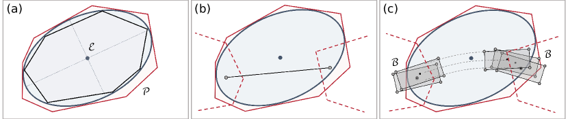
Figure 4: Demonstration of geometric constraints for an ellipsoid (blue). (a) The general formulation of inner and outer Löwner-John ellipsoid. (b) The Inner Löwner-John ellipsoid with outer line segment constraints. (c) The Inner Löwner-John ellipsoid with outer convex bodies constraints. The dash shapes represent neighbored polytopes.

Given current waypoints $p^{k}$, we can formulate the sub-problem of finding the $i$-th ellipsoid by

$$\min_{L_{i},d_{i}}\ -w_{v}\log\det(L_{i})+\frac{\rho}{2}\|[g(h_{0}(\mathcal{E}_{i},p_{i}^{k})),g(h_{0}(\mathcal{E}_{i},p_{i-1}^{k}))]^{T}+y_{i}^{k}\|_{2}^{2},$$ (14a)

$${\rm s.t.}\ \ \|(a_{i,j})^{T}L_{i}\|_{2}+(a_{i,j})^{T}d_{i}\leq b_{i,j},\ \ j=1,\cdots,v_{i}$$ (14b)

$$L_{i}\ {\rm is\ lower\ triangular},\ \ \$$ (14c)

where the first term of objective, $\log\det(L_{i})$, is proportional to the volume of the ellipsoid, and (14b) represents corridor constraints. We employ a distributed style to update $\mathcal{E}^{k+1}$.

5 Results

5.1 Implementation Details

We use the procedure developed in [26] which defines a quantity called the Environmental Complexity Signature (ECS) to generate environments of varying complexities (obstacle structures, densities, etc). All environments are stored as voxel maps. We use the RRT* [2] algorithm from the OMPL library [32] to get the initial geometric path for all methods. We use the L-BFGS algorithm [33] to minimize the augmented Lagrangian for all the constrained optimization problems in our approach. We therefore replace hard constraints with soft ones, but we do not perform a dual update step in our approach. In practice, we run the inner iteration once and update the polytope through several outer iterations. Our approach can be deployed on our custom hardware platform [34] to provide an environmental representation for two-stage motion planning.

5.2 Numerical Analysis

We conduct several tests in a parameterized environment of size 20 $\times$ 20 $\times$ 5 m³ with randomly chosen start and end points, at least 10 m apart. All obstacles are inflated by the radius of the robot. We use total volumes of ellipsoids ($vol(\mathcal{E})$) and polytopes ($vol(\mathcal{P}))$, and overlapping volumes of each neighboring pair of polytopes ($vol(\cap\mathcal{P}))$ to showcase the performance of the proposed algorithm during several iterations. For evaluation among different test cases, the values were normalized by the maximum values observed during the iterations of a trial.

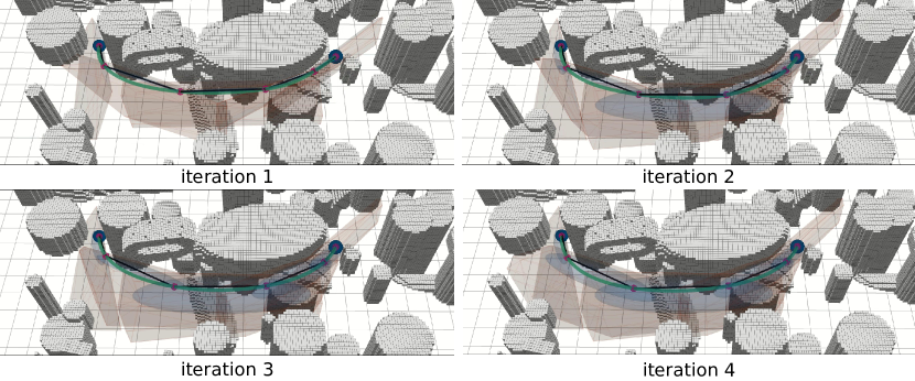
Figure 5: Visualization of ellipsoids (blue) and polytopes (red) during 4 iterations. The black line segments represent the path, with waypoints in magenta. The green curve is the trajectory generated within polytopes.

5.2.1 Ellipsoids and Polytopes over Iterations.

To validate the effectiveness of our proposed method, we show one example using heuristics $\tilde{J}_{1}$ and visualize the ellipsoids and polytopes of four iterations in Fig.5. The center and orientation (or axes) impact the maximum volume an ellipsoid can inflate, and our proposed method is able to adjust it with iterations. Fig.6 illustrates the actual volumes of additional tests.

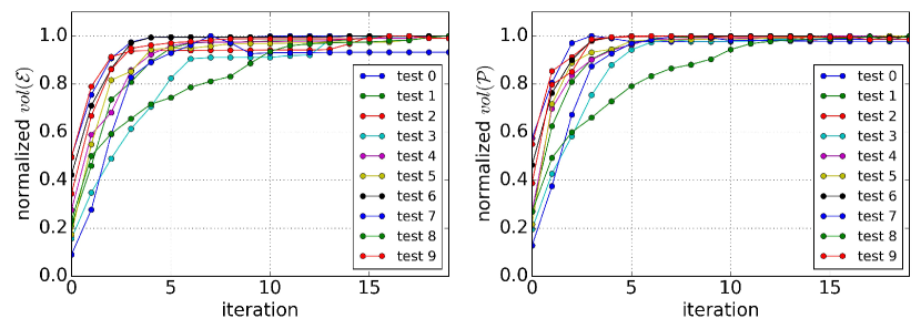
Figure 6: The variance in normalized volumes of ellipsoids and polytopes after 20 iterations of our proposed algorithm (across ten trials).

The normalized volumes of ellipsoids (left) and polytopes (right) consistently grow with each iteration and contain more than 90% of the maximum volumes within 5-10 iterations in most cases. In what follows, we will cap the number of iterations between 5 and 10; we empirically observed that this comes without sacrificing performance.

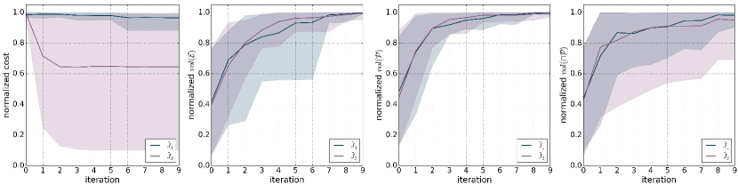
Figure 7: Comparison of performance by trajectory heuristics based on minimum path length ($\tilde{J}_{1}$) and minimum control effort ($\tilde{J}_{2}$) over 100 test cases.

5.2.2 The Effects of Cost Heuristics.

We compare two trajectory heuristics with minimum path length and minimum control effort (using jerk) for waypoint updates and show the dependence of normalized volumes of ellipsoids, polytopes, and overlapping areas of the convex cover with the number of iterations. We use a uniform time allocation proportional to the path length in minimum control effort to ensure that the waypoints are distributed uniformly as they move and that the cost term is updated consistently. The performances using different trajectory heuristics costs are shown in Fig.7. The cost $\tilde{J}_{2}$ performs slightly better than $\tilde{J}_{1}$, regarding the coverage rate of ellipsoids and polytopes volumes. The cost value of distance has less margin to decrease as the initial path from RRT* has already minimized the distance to a large extent.

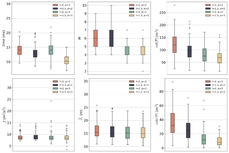
Figure 8: Performance by different distinct settings with $l\in\{1.5,2\}$ and $\alpha\in\{2,3\}$.

5.2.3 Configurable Performance in Different Environments

We leverage parameters such as local range $l$ and upsample threshold $\alpha$ to generate SFC with specified accuracy and efficiency. Our analysis considers the following four setups with a local range of 1.5 m and 2.0 m and an upsample threshold of 2.0 m and 3.0 m. The upsample threshold influences the number of segments, and the local range determines the number of obstacles considered for each polytope generation. These settings are evaluated in terms of computation time, trajectory cost ($J$), number of segments ($M$), path length ($\tilde{J}_{1}$), and volumes of ellipsoids, polytopes, and overlapping areas. Trajectory cost is evaluated by optimizing time intervals and waypoints in [35]. As shown in Fig.8, the computation time can be reduced by decreasing the local range and increasing the upsample threshold. The path length, polytope volumes, overlapping volumes, and trajectory cost also decrease accordingly. We conclude that within the same homotopic class, the optimal trajectory is indeed influenced by the convex cover.

5.3 Comparison of Convex Cover

We compare our proposed algorithm with two state-of-the-art SFC generation methods, IRIS[3] and the method presented in [8], denoted as RILS. IRIS was originally designed for graph cover, and we use its applications for a convex cover of a path with incremental point collision checking. The iteration number of IRIS is set as the major iteration in their paper, the same as our proposed method. To get inner Löwner-John ellipsoids in IRIS, we directly employ the Cholesky representation for optimization in [7]. We evaluate the performance of three methods across various randomized environments with dimensions of $30\times 30\times 5\$m³ characterized by the ECS (density index, cluster index, and structure index). We conduct 10000 tests within these environments, randomly selecting start and end points with a distance threshold of 5 m. The results are filtered to exclude all invalid cases encountered by any of the methods.

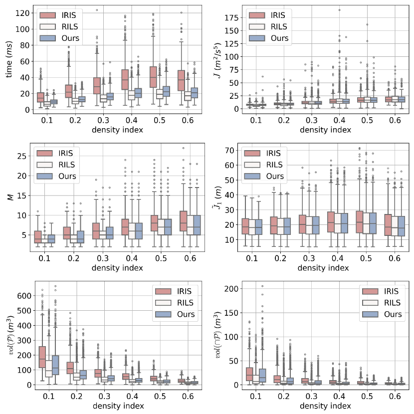
Figure 9: Benchmark comparisons with increasing density index (defined in [26]).

We categorize test cases based on the range of the density index to represent environment complexity and show the results in Fig. 9. As the density index increases, environments become more complex, which leads to reduced polytope volumes and decreased trajectory performance across all three methods. When the density index exceeds 0.5, finding a feasible geometric path over long distances becomes challenging, resulting in shorter paths and fewer segments. Our method updates the path for better trajectory generation, particularly in complex environments such as narrow mazes where RILS show poor performance around corners, illustrated in Fig. 10.

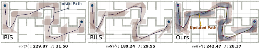
Figure 10: The illustration of SFC generated by three methods.

Benchmark results classified by start-end distance (the Euclidean distance between the start to end point) are demonstrated in Fig. 11. As the start-to-end distance increases, our method demonstrates improved performance in terms of computation time, trajectory cost, and path length. It is clear that the performance of any algorithm depends on the complexity of the environment and start-to-end distance, and it is difficult to draw conclusions based on average performance. However, as shown in Fig. 9 and 11, the worst-case cost for our proposed method is lower than that obtained by RILS and IRIS with similar computational time. More importantly, this is the first systematic analysis of multiple factors that influence the trajectory cost: the waypoint and number of segments in the front-end plan, the volumes of the polytopes in the convex cover, and the volumes of consecutive polytopes.

6 Conclusion and Future Work

This paper introduces a novel algorithm to find an optimal convex cover of collision-free space as SFC for trajectory optimization.

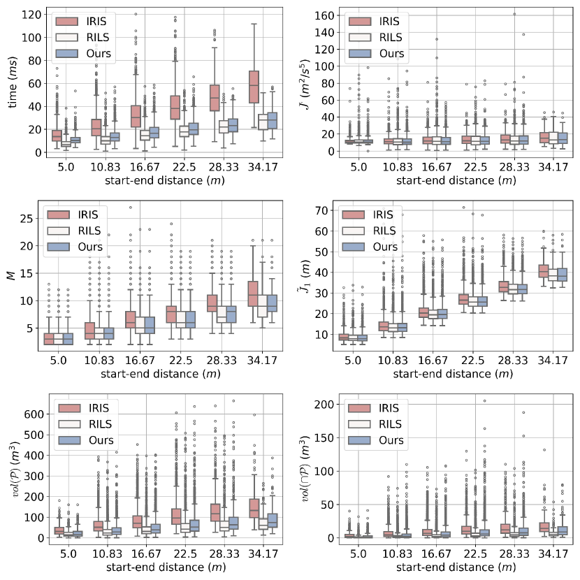
Figure 11: Benchmark comparisons with increasing start-end distance.

The convex cover is formulated as a joint optimization of ellipsoids, polytopes, and intermediate waypoints, which are updated iteratively to find optimal solutions.

The proposed method can be applied to two-stage motion planning as an intermediate process, or optimizing with trajectory generation jointly. Furthermore, we will extend our method to whole-body SE(n) trajectory planning with an initial set of rigid bodies.

References

- [1] S. M. LaValle. Planning Algorithms. Cambridge University Press, Cambridge, U.K., 2006. Available at http://planning.cs.uiuc.edu/.
- [2] Sertac Karaman and Emilio Frazzoli. Sampling-based algorithms for optimal motion planning. The International Journal of Robotics Research, 30:846–894, 2011.
- [3] Robin Deits and Russ Tedrake. Computing large convex regions of obstacle-free space through semi-definite programming. In Algorithmic Foundations of Robotics XI: Selected Contributions of the Eleventh International Workshop on the Algorithmic Foundations of Robotics (WAFR), pages 109–124, 2015.
- [4] Fei Gao and Shaojie Shen. Online quadrotor trajectory generation and autonomous navigation on point clouds. In 2016 IEEE International Symposium on Safety, Security, and Rescue Robotics (SSRR), pages 139–146, 2016.
- [5] Mukulika Ghosh, Shawna Thomas, and Nancy M. Amato. Fast collision detection for motion planning using shape primitive skeletons. In Marco Morales, Lydia Tapia, Gildardo Sánchez-Ante, and Seth Hutchinson, editors, Algorithmic Foundations of Robotics XIII, pages 36–51, Cham, 2020. Springer International Publishing.
- [6] Xingguang Zhong, Yuwei Wu, Dong Wang, Qianhao Wang, Chao Xu, and Fei Gao. Generating large convex polytopes directly on point clouds. arXiv preprint arXiv:2010.08744, 2020.
- [7] Qianhao Wang, Zhepei Wang, Chao Xu, and Fei Gao. Fast iterative region inflation for computing large 2-d/3-d convex regions of obstacle-free space, 2024.
- [8] Sikang Liu, Michael Watterson, Kartik Mohta, Ke Sun, Subhrajit Bhattacharya, Camillo J. Taylor, and Vijay Kumar. Planning dynamically feasible trajectories for quadrotors using safe flight corridors in 3-d complex environments. IEEE Robotics and Automation Letters, 2(3):1688–1695, 2017.
- [9] Yuwei Wu, Ziming Ding, Chao Xu, and Fei Gao. External forces resilient safe motion planning for quadrotor. IEEE Robotics and Automation Letters, 6(4):8506–8513, 2021.
- [10] Zhepei Wang, Chao Xu, and Fei Gao. Robust trajectory planning for spatial-temporal multi-drone coordination in large scenes. In 2022 IEEE/RSJ International Conference on Intelligent Robots and Systems (IROS), pages 12182–12188, 2022.
- [11] Stephen Boyd, Neal Parikh, Eric Chu, Borja Peleato, and Jonathan Eckstein. Distributed optimization and statistical learning via the alternating direction method of multipliers. Foundations and Trends® in Machine Learning, 3(1):1–122, 2011.
- [12] Bernard M. Chazelle. Convex decompositions of polyhedra. In Proceedings of the Thirteenth Annual ACM Symposium on Theory of Computing, STOC ’81, page 70–79, New York, NY, USA, 1981. Association for Computing Machinery.
- [13] Jyh-Ming Lien and Nancy M. Amato. Approximate convex decomposition of polyhedra. In Proceedings of the 2007 ACM Symposium on Solid and Physical Modeling, SPM ’07, page 121–131, New York, NY, USA, 2007. Association for Computing Machinery.
- [14] Xinyue Wei, Minghua Liu, Zhan Ling, and Hao Su. Approximate convex decomposition for 3d meshes with collision-aware concavity and tree search. ACM Transactions on Graphics (TOG), 41(4):1–18, 2022.
- [15] Boyang Deng, Kyle Genova, Soroosh Yazdani, Sofien Bouaziz, Geoffrey Hinton, and Andrea Tagliasacchi. Cvxnet: Learnable convex decomposition. In 2020 IEEE/CVF Conference on Computer Vision and Pattern Recognition (CVPR), pages 31–41, 2020.
- [16] Jing Chen, Tianbo Liu, and Shaojie Shen. Online generation of collision-free trajectories for quadrotor flight in unknown cluttered environments. In 2016 IEEE International Conference on Robotics and Automation (ICRA), pages 1476–1483, 2016.
- [17] Tobia Marcucci, Parth Nobel, Russ Tedrake, and Stephen Boyd. Fast path planning through large collections of safe boxes, 2024.
- [18] Aaron Ray, Alyssa Pierson, and Daniela Rus. Free-space ellipsoid graphs for multi-agent target monitoring. In 2022 International Conference on Robotics and Automation (ICRA), pages 6860–6866, 2022.
- [19] Yunfan Ren, Fangcheng Zhu, Wenyi Liu, Zhepei Wang, Yi Lin, Fei Gao, and Fu Zhang. Bubble planner: Planning high-speed smooth quadrotor trajectories using receding corridors. In 2022 IEEE/RSJ International Conference on Intelligent Robots and Systems (IROS), pages 6332–6339, 2022.
- [20] Peter Werner, Alexandre Amice, Tobia Marcucci, Daniela Rus, and Russ Tedrake. Approximating robot configuration spaces with few convex sets using clique covers of visibility graphs, 2024.
- [21] Fei Gao, Luqi Wang, Boyu Zhou, Xin Zhou, Jie Pan, and Shaojie Shen. Teach-Repeat-Replan: A complete and robust system for aggressive flight in complex environments. IEEE Transactions on Robotics, 36(5):1526 – 1545, 2020.
- [22] Fritz John. Extremum Problems with Inequalities as Subsidiary Conditions, pages 197–215. Springer Basel, Basel, 2014.
- [23] Sergei Savin. An algorithm for generating convex obstacle-free regions based on stereographic projection. In 2017 International Siberian Conference on Control and Communications (SIBCON), pages 1–6, 2017.
- [24] Robin Deits and Russ Tedrake. Efficient mixed-integer planning for uavs in cluttered environments. In 2015 IEEE International Conference on Robotics and Automation (ICRA), pages 42–49, 2015.
- [25] Tobia Marcucci, Jack Umenberger, Pablo Parrilo, and Russ Tedrake. Shortest paths in graphs of convex sets. SIAM Journal on Optimization, 34(1):507–532, 2024.
- [26] Yifei Simon Shao, Yuwei Wu, Laura Jarin-Lipschitz, Pratik Chaudhari, and Vijay Kumar. Design and evaluation of motion planners for quadrotors in environments with varying complexities, 2024.
- [27] Stephen Boyd and Lieven Vandenberghe. Convex optimization. Cambridge university press, 2004.
- [28] Daniel Mellinger and Vijay Kumar. Minimum snap trajectory generation and control for quadrotors. In 2011 IEEE International Conference on Robotics and Automation, pages 2520–2525, 2011.
- [29] Weidong Sun, Gao Tang, and Kris Hauser. Fast uav trajectory optimization using bilevel optimization with analytical gradients. In 2020 American Control Conference (ACC), pages 82–87, 2020.
- [30] Yuwei Wu, Xiatao Sun, Igor Spasojevic, and Vijay Kumar. Deep learning for optimization of trajectories for quadrotors. IEEE Robotics and Automation Letters, 9(3):2479–2486, 2024.
- [31] Charles Richter, Adam Bry, and Nicholas Roy. Polynomial trajectory planning for aggressive quadrotor flight in dense indoor environments. In Robotics Research: The 16th International Symposium ISRR, pages 649–666. Springer, 2016.
- [32] Ioan A. Şucan, Mark Moll, and Lydia E. Kavraki. The Open Motion Planning Library. IEEE Robotics & Automation Magazine, 19(4):72–82, December 2012. https://ompl.kavrakilab.org.
- [33] Dong C Liu and Jorge Nocedal. On the limited memory bfgs method for large scale optimization. Mathematical programming, 45(1-3):503–528, 1989.
- [34] Yuezhan Tao, Yuwei Wu, Beiming Li, Fernando Cladera, Alex Zhou, Dinesh Thakur, and Vijay Kumar. Seer: Safe efficient exploration for aerial robots using learning to predict information gain. In 2023 IEEE International Conference on Robotics and Automation (ICRA), pages 1235–1241, 2023.
- [35] Zhepei Wang, Xin Zhou, Chao Xu, and Fei Gao. Geometrically constrained trajectory optimization for multicopters. IEEE Transactions on Robotics, 38(5):3259–3278, 2022.