Automated Molecular Concept Generation and Labeling with Large Language Models

Abstract

Artificial intelligence (AI) is significantly transforming scientific research. Explainable AI methods, such as concept-based models (CMs), are promising for driving new scientific discoveries because they make predictions based on meaningful concepts and offer insights into the prediction process. In molecular science, however, explainable CMs are not as common compared to black-box models like Graph Neural Networks (GNNs), primarily due to their requirement for predefined concepts and manual label for each instance, which demand domain knowledge and can be labor-intensive. This paper introduces a novel framework for Automated Molecular Concept (AutoMolCo) generation and labeling. AutoMolCo leverages the knowledge in Large Language Models (LLMs) to automatically generate predictive molecular concepts and label them for each molecule. Such procedures are repeated through iterative interactions with LLMs to refine concepts, enabling simple linear models on the refined concepts to outperform GNNs and LLM in-context learning on several benchmarks. The whole AutoMolCo framework is automated without any human knowledge inputs in either concept generation, labeling, or refinement, thereby surpassing the limitations of extant CMs while maintaining their explainability and allowing easy intervention. Through systematic experiments on MoleculeNet and High-Throughput Experimentation (HTE) datasets, we demonstrate that the AutoMolCo-induced explainable CMs are beneficial and promising for molecular science research.

1 Introduction

Artificial intelligence (AI) has been a driving force behind several groundbreaking scientific discoveries, particularly in the domain of molecular science. A prime example is the utilization of deep learning by the MIT Jameel Clinic, leading to the identification of halicin – the first antibiotic discovered in three decades that is effective against a broad spectrum of 35 bacteria [33]. In molecular science, deep learning models like Graph Neural Networks (GNNs) have shown promising capabilities for learning complex atomic structures and making accurate predictions of molecular properties [36]. However, a major challenge with such deep-learning-based models like GNNs is their “black boxes” nature and lack of explainability [42]. Despite their high predictive performance, black-box models fail to provide insights into the underlying reasoning behind their predictions, making it difficult for scientists to interpret and intervene in the model’s decision-making process, which hinders scientific understanding and limits the potential for knowledge discovery.

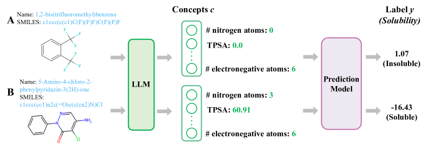
Figure 1: The prediction process of molecule properties is greatly illuminated with AutoMolCo. First, concepts are generated and labeled with an LLM. Afterward, a simple prediction model (e.g., linear regression) can be fitted to achieve explainable predictions. LLM-relevant pieces are highlighted in green, and specifically, green arrows indicate prompting.

In contrast, concept-based models (CMs) [20, 19, 38, 35] have emerged as a promising explainable AI (XAI) solution for scientific problems, whose explainability can provide valuable insights and increase the chance of new scientific discoveries. Unlike other black-box models, CMs first predict labels of human-interpretable concepts from the data and then use these concept labels as features to predict the actual task label. For example, in computer vision, CMs are applied for predicting the species of birds from their images by identifying the relevant concepts like “wing color”, which greatly increases the prediction explainability [19]. In molecular science, CMs can be especially beneficial as they can break down the prediction of complex molecular properties into more interpretable molecular concepts like functional groups and molecular descriptors. For instance, Figure 1 demonstrates the prediction process of a CM for molecules A and B. The CM first elucidates the relevant molecular descriptors as concepts, such as the # of nitrogen atoms and the topological polar surface area (TPSA), which are further employed to predict the molecule’s solubility. This process not only yields a prediction but also provides a rationale that can be scrutinized and built upon. Like molecule B is predicted to be soluble based on its high TPSA, researchers can explore similar molecules with slight variations in these key concepts to hypothesize and test solubility-enhancing modifications. In contrast, black-box models, while potentially accurate, offer no such explanatory power.

Despite being a promising XAI approach, CMs have not been widely applied to molecular science problems, primarily due to their limitations in concept generation and labeling. Extant CM approaches either require predefined concepts and manual labels generated by domain experts [19] or can only utilize simple and qualitative concepts that are insufficient for molecular problems [27]. Collecting such concepts and their labels is feasible and adequate for some computer vision tasks [19, 27]. However, the desired concepts for molecules are sophisticated and nuanced, which require a depth of chemical knowledge and accurate quantitative labels. For example, TPSA in Figure 1 is a molecule descriptor relevant to the solubility prediction. It provides insight into a molecule’s absorption and permeability characteristics, representing a quantitative concept pivotal for understanding the pharmacokinetics of potential drug compounds. Identifying and quantifying such a concept often demands domain knowledge and computational methods that extant CM approaches cannot achieve, thereby highlighting the challenge in effective CMs for molecular sciences.

In response to the effectiveness of CMs and the challenges of applying them to molecular science, we propose Automated Molecular Concept (AutoMolCo) generation and labeling. AutoMolCo leverages Large Language Models (LLMs) to generate molecular concepts that are predictive for the task and label these concepts for each molecule instance. AutoMolCo also repeats these procedures through iterative interactions with LLMs to refine concepts, enabling simple linear models on the refined concepts to outperform GNNs and LLM in-context learning (ICL) on several molecular benchmarks. The whole AutoMolCo framework is automated and does not require human knowledge inputs in either concept generation, labeling, or refinement, thus surpassing the limitations of extant CMs.

The motivation of AutoMolCo is founded on the idea that LLMs can be treated as extensive and integrated knowledge bases [30, 4], and their effectiveness for solving molecular science problems has been benchmarked in [13] through ICL. In our work, we exploit the potential of LLMs for XAI through CMs. For concept generation, we prompt LLMs with the task description and ask LLMs to suggest relevant concepts. For concept labeling, since it is particularly challenging, we explore three different approaches: direct LLM prompting, function code generation, and external tool calling. The concept generation and labeling process form the foundation of our framework. Afterward, we fit simple prediction models on the concepts to achieve an explainable CM. Moreover, we also do an iterative refinement of the concepts by running feature selection algorithms of the prediction model and prompting LLMs again with the feature selection results. This allows LLMs to generate new concepts to replace the less useful ones from the previous iteration, which ensures the CM remains up-to-date with the most relevant concepts thus boosting its performance.

In this work, we first show that AutoMolCo can produce meaningful concepts and accurate labels, which lead to CMs with simple prediction models to achieve surprisingly good performance for molecular science problems. Then we perform a systematic study via experiments on MoleculeNet [36] and High-Throughput Experimentation (HTE) [1, 31] datasets to show the strengths and weaknesses of AutoMolCoand answer five research questions. In summary, our contribution includes:

1. Automated framework: We propose AutoMolCo, which leverages LLMs for automated concept generation and labeling, eliminating the need for human domain knowledge and labor-intensive data collection, thereby streamlining the development of CMs.

2. Accuracy and explainability: AutoMolCo produces meaningful molecular concepts that, when combined with simple prediction models for CMs, can achieve superior or comparable accuracy to powerful black-box models while providing greater explainability.

3. LLM-driven XAI for science: Our work highlights the potential of LLMs in addressing complex problems in molecular science, introduces a novel perspective on CMs with LLMs, and paves the way for future research to further exploit the capabilities of LLMs in molecular science and beyond.

2 Related work

Concept-based Models. A popular example of CMs is the Concept Bottleneck Model (CBM) [19]. CBMs make predictions through an intermediate layer of human-specified concepts, such as “wing color” in specious classification from bird images. While CBMs offer more transparent predictions, they are often constrained by the predefined concepts and label demands. Several follow-up CBMs with predefined concepts targeting different tasks [10, 39, 7, 23, 8]. One particular follow-up that is more relevant to this work, label-free CBM [27], tries to bypass the need for predefined concepts and labels by generation and similarity matching. Unlike the other CBMs, this model identifies concepts using GPT-3 for concept set creation and CLIP-Dissect for matching text concepts with images. However, label-free CBM only focuses on vision tasks, and the generated concepts are often simple and qualitative, e.g., “yellow” is a concept, with similarity as the label, e.g., how similar a “lemon” image is to the text “yellow”. Such concepts and labels are insufficient for molecules, where a depth of chemical knowledge is required for meaningful concepts and accurate qualitative labels.

Concept Learning in Graphs/Molecule. Several lines of research study concept learning from graph data, particularly for molecules. One line identifies graph motifs as concepts through counting or sampling [26, 34] and builds GNNs on top of them [44, 41]. However, motif identification cannot be comprehensive as it is NP-complete. Another line tries to use concept-based explanations for GNNs with human-in-the-loop, e.g., GCExplainer [24]. Subsequent works have refined this idea with k-means clustering and similarity scoring algorithms to neuron-level grouping within activation layers [25, 37]. These methods exemplify the attempt to extract and interpret salient features in graph data, yet they often face challenges in fully capturing the nuanced complexity of molecular structures.

LLMs for Molecular Science. GPT4Graph [12] prompts LLMs to explain the format or to summarize a raw molecule graph input, where the graph is represented by the Graph Modelling Language (GML) [16] or Graph Markup Language (GraphML) [6]. Graph-ToolFormer [43] lets LLMs generate API calls to use external graph reasoning tools, which can be applied to molecule function reasoning problems. [13] studies solving molecular problems with LLMs ICL. We show our AutoMolCo outperforms ICL and enjoys better explainability. Some other survey papers discussing the potential of LLMs for molecular science include: [45] from a scientific research perspective and [18] from an LLM for graph perspective, and [40] for fine-tuning LLMs.

3 AutoMolCo: automated molecular concept generation and labeling

In this section, we describe AutoMolCo for concept generation, labeling, and refinement, where the concepts are used to build an explainable CM. Figure 2 depicts the three major steps of AutoMolCo: 1) concept generation, 2) concept labeling, and 3) CM fitting and concept selection.

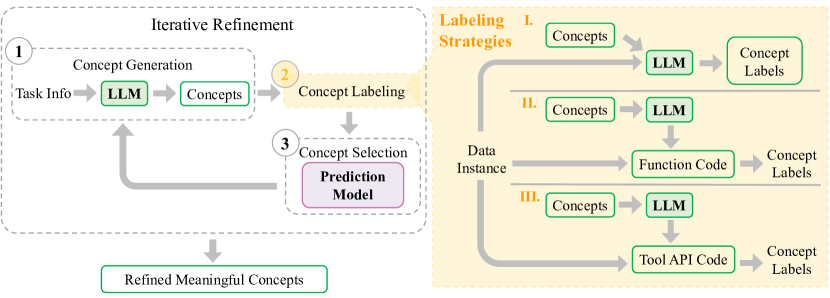
Figure 2: The AutoMolCo framework. Step 1: concept generation. Step 2: concept labeling with three different strategies. Step 3: fitting a prediction model and perform concept selection. These three steps are repeated for multiple iterations to achieve a refined list of meaningful concepts, where the selected concepts in each iteration are feedback to the LLM through prompting. LLM outputs are highlighted as green boxes.

Step 1: Concept Generation Given a particular task on molecules, e.g., predicting the hydration-free energy of small molecules in water, the first step is to prompt LLMs to propose a diverse list of concepts that are potentially relevant to the task. This step is analogous to a brainstorming process. Concepts range from counting-based ones, like # nitrogen atoms, to more complicated ones that require precise calculation, like TPSA. Without LLMs, coming up with meaningful concepts requires domain experts. The underlying intuition for concept generation is founded on the idea that LLMs can be treated as extensive and integrated knowledge bases. Their capacity to comprehend and output meaningful concepts is pivotal in this phase, yielding a wide spectrum of potentially relevant concepts for our analysis. The prompt for this step is shown in Figure 3 Step 1. The LLM-suggested concepts might be less relevant initially, but they will be refined later.

Step 2: Concept Labeling Following the concept generation step, we then label the generated concepts for each data instance. Compared to human labeling, which requires domain knowledge and can be labor-intensive. Labeling with LLMs is streamlined to a process of interaction with a single LLM interface, which can be easily scaled and minimizes human error. This automation with LLMs is crucial for efficiently processing large volumes of data encountered in molecular studies. In this step, we consider three different labeling strategies to enhance labeling quality.

Labeling Strategy 1: Direct LLM prompting We prompt LLMs directly to assign each data instance numerical or categorical labels for the generated concepts from Step 1. Similar to concept generation, this strategy builds up on the idea that LLMs can be treated as integrated knowledge bases for retrieving useful information. For each data instance, we provide LLMs with the molecule names or SMILES strings. The prompt is shown in Figure 3 Step 2.

Labeling Strategy 2: Function code generation with LLMs Since LLMs are particularly skilled in code generation, we explore a second approach for concept labeling: generate functions in Python code for computing the concept labels. The function generation approach has two advantages. Firstly, it greatly reduces the need for repeated LLM API calls. Only a single API call is required for each concept to obtain the function code, as opposed to making a separate call for each data instance in the direct label prompting case. Secondly, the generated functions can utilize preprocessed dataset features as function arguments, such as atom types in terms of node features and molecule structures in terms of adjacency matrix. These features provide more direct information beyond molecule names or SMILES strings. Leveraging these features, the LLM-generated functions can offer more nuanced and accurate concept labels, enhancing the effectiveness of AutoMolCo. The prompt is shown in Figure 7 in Appendix A.

Labeling Strategy 3: External tool calling with LLMs We also utilize LLMs to call external tools like RDKit [21] for labeling, combining the generation ability of LLMs with the reliability of specialized tools. This strategy enjoys the same efficiency advantage as the function generation approach, meaning it requires only a single API call of the LLM per concept to get the API code for calling the tool. Moreover, the use of labeling tools ensures that labels for all the tool-calculable concepts are accurate and reliable. One disadvantage of this strategy is that not all generated concepts are calculable by the external tool, in which case we can only turn to the first two strategies. The prompt is shown in Figure 8 in Appendix A.

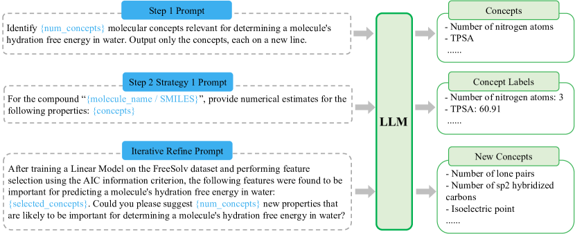
Figure 3: Prompts for concept generation and labeling on the FreeSolv dataset. Hyperparameters, molecule instance information, and re-used LLM responses from a previous step are in blue.

Step 3: CM Fitting and Concept Selection After getting the generated concepts and their labels, we utilize them to fit prediction models for the molecular task. Since the concept labels can be treated as tabular data, any model from the off-the-shelf ones in Scikit-learn [29] to sophisticated deep learning models can be applied. However, we found that explainable models like linear models and decision trees or simple two-layer multi-layer perceptions (MLPs) are often sufficient for achieving competitive performance. We attribute the credit to the high-quality concepts and their labels. We will discuss our model choice and perform a systematic study of different prediction models in Section 4. While fitting the model, we also run feature selection methods like Akaike Information Criterion (AIC) [2, 3] and Recursive Feature Elimination (RFE) [15] to determine the useful concepts. Feature selection not only boosts the model performance but also leads to automated iterative refinement for identifying a list of the most useful concepts.

Iterative Concepts Refinement After all three steps. We do an iterative refinement of the generated concepts by prompting LLMs again with the empirical performance of our prediction model and the concept selection results from Step 3. We include such information in an updated prompt to make LLMs generate new concepts to replace the less useful ones from the previous iteration. Using the empirical results as feedback, we ensure that our CM remains adaptable and up-to-date with the most relevant molecular concepts. Through this iterative refinement process, we guarantee that the model performance improves over iterations and prune the irrelevant concepts generated in previous iterations. The prompt for this step is shown in Figure 3.

4 Experiments

4.1 Experiment settings

Datasets We include four datasets from MoleculeNet [36]. Two regression datasets, e.g., FreeSolv and ESOL, and two classification datasets, e.g., BBBP and BACE. FreeSolv provides hydration-free energy (which induces solubility) for 642 molecules, while ESOL contains water solubility data for 1128 organic small molecules. BBBP contains 2,039 molecules and assesses compounds’ blood-brain barrier penetration. BACE has 1,513 molecules and predicts $\beta$-secretase 1 inhibitors, relevant for Alzheimer’s research. For all datasets, we employed the same scaffold splits as the Open Graph Benchmark (OGB) [17]. We also include two HTE datasets, e.g., Buchwald-Hartwig (BH) [1] and Suzuki-Miyaura (SM) [31] for chemical reaction yield prediction. BH provides the yields of the Buchwald-Hartwig reaction for 3957 molecules, and SM provides the yield of the Suzuki reaction for 5650 molecules. We employed the same data splits as used in [13].

Metrics We follow the standard evaluation metrics for these datasets. For FreeSolv and ESOL, results are measured with Root Mean Square Error (RMSE). For BBBP and BACE, we mainly evaluate these datasets using AUC-ROC and report results in our main Table 1. Since [13] evaluates BBBP and BACE with accuracy, we also report a comparison in accuracy in Table 7 in Appendix F. For BH and SM, we evaluate with accuracy.

Baselines Our baselines include GNNs, LLM ICL, and GNN + CBM. Specifically, we use the GIN and GCN. For LLM ICL, we reference the findings from [13] and use their prompts. For GNN + CBM, we use GIN and use GPT-3.5 Turbo for generating concept labels for CBM. For HTE datasets, we only consider LLM ICL baselines as graphs are not provided for the test set.

Models We employ GPT-3.5 Turbo as our primary LLMs for generating concepts and directly labeling. Additionally, we utilize GPT-4 for labeling strategy 2: function code generation, and strategy 3: external tool calling. For strategy 3, the LLM will create code snippets for invoking RDKit [21]. We don’t use GPT-4 for direct labeling due to the high cost of per-instance labeling. After collecting the concept labels, we explore four types of prediction models to cover a broad spectrum of tasks and performance levels. As a basic setting, we use linear models like linear regression and logistic regression, we also consider more advanced models including decision trees and 2-layer MLPs. We use off-the-shelf prediction models from sklearn [29]. We do ablation on LLMs with Claude-2 in Appendix E. Since we call LLMs through their APIs and the prediction models are light and off-the-shelf, there is no specially requirements, like GPUs, for our framework.

Concept Selection We employ AIC [2, 3] for regression and RFE [14] for classification. These selection methods are specifically applied to linear models. For multi-iteration performance with decision trees and MLPs, we use the selection results from the linear models.

4.2 AutoMolCo-induced CM performance

In Table 1, we compare the performance of the AutoMolCo-induced CM to baselines. Compared to GNNs, our CM achieves better results on MoleculeNet regression tasks and HTE tasks and competitive results on MoleculeNet classification tasks. In comparison to the results presented by ICL, our models have demonstrated a substantial performance advantage on all tasks. Our best-performing model is the culmination of multiple iterations of refinement and a combination of labeling strategies. Specifically, the results presented in Table 1 are achieved using the following approaches: 1. A combination of all three labeling strategies for concept labeling, with further details provided in Appendix E.3 2. The optimal CMs from linear models, decision trees, and MLPs 3. Concepts refinement over three iterations, as discussed in Section 4.6. An in-depth exposition of these techniques is discussed in detail in the RQs below through experiments on MoleculeNet datasets. More details on experiment results for HTE datasets are shown in Appendix H.

Table 1: Performance comparison of the AutoMolCo-induced CM with baselines. MoleculeNet regression tasks (FreeSolv and ESOL) are measured in RMSE ($\downarrow$). MoleculeNet classification tasks (BBBP and BACE) are measured in AUC-ROC ($\uparrow$). HTE datasets (BH and SM) are measured in accuracy ($\uparrow$). Ours achieve better results on MoleculeNet regression and HTE tasks and competitive results on MoleculeNet classification tasks.

	FreeSolv ($\downarrow$)	ESOL ($\downarrow$)	BBBP ($\uparrow$)	BACE ($\uparrow$)	BH ($\uparrow$)	SM ($\uparrow$)
GIN	2.151	0.998	69.710	73.460	-	-
GCN	2.186	1.015	67.800	68.930	-	-
GIN + CBM	2.412	1.373	54.500	68.457	-	-
GPT-3.5 Turbo (zero-shot)	5.450	2.039	49.256	48.765	0.320	0.473
GPT-3.5 Turbo (4-shot)	4.852	1.161	51.580	41.871	0.640	0.630
GPT-3.5 Turbo (8-shot)	4.491	1.128	56.632	47.757	0.706	0.693
AutoMolCo-CM (ours)	2.065	0.843	65.278	70.744	0.810	0.800

4.3 RQ1: Can AutoMolCo generate meaningful molecular concepts?

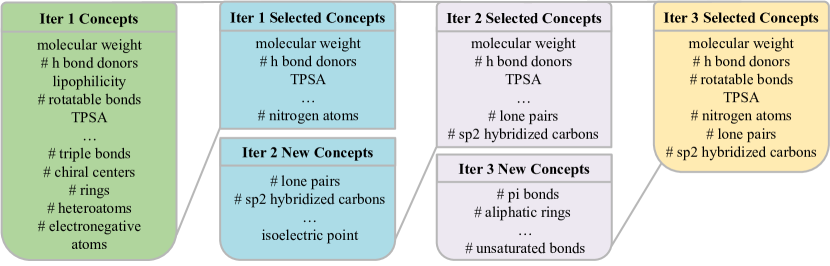
Figure 4: RQ1: Concepts selected by AutoMolCo in three refinement iterations on FreeSolv. A detailed version in Appendix B Figure 9.

The effectiveness of the CM is built on meaningful concepts, which used to rely on domain experts [19]. In this RQ1, we examine the concepts generated by AutoMolCo in each refinement iteration and consult with domain experts for their rationality. Figure 4 shows the concepts selected by a linear regression model for predicting solubility (FreeSolv), evolving from an initial broad set to a more focused and chemically relevant set. According to our consultation with domain experts, the eliminated concepts such as the counts of specific atoms and rotatable bonds, while informative, may not have significantly contributed to the model’s predictive power or may have been correlated with other concepts. The retained concepts, like molecular weight, # hydrogen bond donors, and TPSA, are fundamental properties that influence molecular interaction and behavior in a solvent. For instance, hydrogen bond donors directly relate to a molecule’s ability to engage in hydrogen bonding, a key interaction for solubility. The TPSA measures the molecule’s surface that can engage in polar interactions, which is crucial for solubility in polar solvents [28]. Thus, the final selected concepts are indeed more chemically meaningful for the task and align with domain knowledge.

4.4 RQ2: Can AutoMolCo assign molecules reasonable concept labels using each strategy?

Accurate concept labels are another critical component of CM performance. In this RQ2, we evaluate AutoMolCo labeling results. we collect ground truth labels for concepts where labels are available, either through calculation (e.g., for molecular weights), or manual lookup (e.g., for melting points). We evaluate labels produced by our direct prompting strategy and function generation labeling strategy using the Pearson correlation coefficient ($r$) with the ground truth, due to the scale-invariant nature of the metric. The external tool calling strategy is excluded from this evaluation as tools will always provide correct labels, and the downside of this strategy is that not all the concepts are tool-calculable (e.g., melting points). Results in Table 2 show strong correlations can be achieved on most datasets with AutoMolCo labeling. Nonetheless, variations in correlation underscore the potential for method improvement. In addition to this benchmarking effort, we also discuss several challenges we encountered and overcame in the labeling step, including imputation for missing values, dictionary for unit inconsistency, and Chain-of-Thoughts (CoT) prompts for syntax errors in function code. A more detailed discussion of these studies are in Appendix C.

Table 2: RQ2: Percentage of concepts with a high correlation ($r$ score $\geq$ 0.7) with the ground-truth.

Labeling Strategy	LLM	Molecule Format	FreeSolv	ESOL	BBBP	BACE
Str-1 Direct Prompt	GPT-3.5	Name	0.82	0.63	0.06	-
Str-1 Direct Prompt	GPT-3.5	SMILES	0.82	0.75	0.69	0.22
Str-2 Function	GPT-4	-	1.00	0.79	0.69	0.67

4.5 RQ3: Can AutoMolCo produced concepts and labels be utilized to build an effective CM?

In RQ1, we have verified that the generated concepts are meaningful according to domain experts. In RQ2, we have shown that concept labels are relatively accurately assigned after properly handling potential issues like missing labels and unit inconsistency. In this RQ3, we compare the performance of the AutoMolCo-induced CMs when different predictions models and labeling strategies are adopted. Results in Table 3 show that AutoMolCo can give reasonable performance even with the most basic direct prompting labeling strategy and the simplest linear model. The good performance of different prediction models demonstrates the quality of the concepts and the effectiveness of AutoMolCo.

Table 3: RQ3: Model performance with different labeling strategies and prediction models.

Labeling Strategy	Prediction Model	FreeSolv($\downarrow$)	ESOL ($\downarrow$)	BBBP ($\uparrow$)	BACE ($\uparrow$)
Str-1 Direct Prompt	Linear/Logistic	2.685	1.250	52.836	56.894
Str-1 Direct Prompt	Decision Tree	2.791	1.272	56.887	68.632
Str-1 Direct Prompt	MLP	2.338	1.194	51.794	60.059
Str-2 Function	Linear/Logistic	3.284	1.254	55.671	56.624
Str-2 Function	Decision Tree	2.569	1.238	54.167	55.573
Str-2 Function	MLP	2.805	1.034	58.738	56.894
Str-3 Tool	Linear/Logistic	3.142	1.011	57.350	63.154
Str-3 Tool	Decision Tree	3.750	1.027	55.903	65.658
Str-3 Tool	MLP	1.981	0.911	58.449	60.772

4.6 RQ4: Does iterative refinement boost the performance of AutoMolCo-induced CM?

As one of the most important designs of our AutoMolCo framework, concept refinement helps to identify meaningful important concepts through iterative interactions with LLMs. The concept relevance has been shown to improve in RQ1, but that does not necessarily mean CM performance will also improve. In this RQ4, we run AutoMolCo with three iterative concept refinements on the MoleculeNet datasets with linear prediction models. We show the results in Figure 5, and we observe that the CM prediction performance indeed improved through concept refinement, especially for classification tasks. The improvement for regression tasks is marginal, partially because the performance is already good for regression.

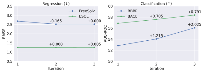
Figure 5: RQ4: Iterative refinement improves CM performance for classification tasks.

4.7 RQ5: Does the AutoMolCo-induced CM facilitates explainable molecular science?

One of the key advantages of CMs over black-box models is their explainability. In this section, we evaluate this aspect of AutoMolCo-induced CMs through three experiments on all three types of the prediction models: coefficient interpretation of linear models, split interpretation of decision trees, and concept label intervention of MLPs.

Coefficient Interpretation of Linear Models Using linears model in the AutoMolCo-induced CM offers excellent explainability through direct interpretation of the model coefficients. We plot the coefficients of the linear model on FreeSolv for predicting hydration free energy in Figure 6 (a), highlighting three significant concepts: # hydrogen bond donors, TPSA, and # rotatable bonds. According to domain experts, the # hydrogen bond donors relates to a molecule’s ability in hydrogen bonding, reflecting its potential to interact with solvents and other molecules. Therefore, an its increment typically leads to a more favorable (more negative) hydration free energy [9]. TPSA quantifies the surface area of a molecule that can engage in polar interactions, providing insights into a molecule’s permeability characteristics. Thus, higher TPSA also leads to more favorable (more negative) hydration free energy [28]. Conversely, the # rotatable bonds positively correlated with hydration free energy. More rotatable bonds increase molecular flexibility, allowing the molecule to adopt conformations that enhance interactions with water molecules. This increased flexibility can lead to less favorable hydration free energy (less negative), as it reduces the stability of the solvation shell around the molecule [11]. Our linear model interpretation aligns with domain knowledge without requiring any human knowledge input into the model. We show results on BBBP in Appendix D.

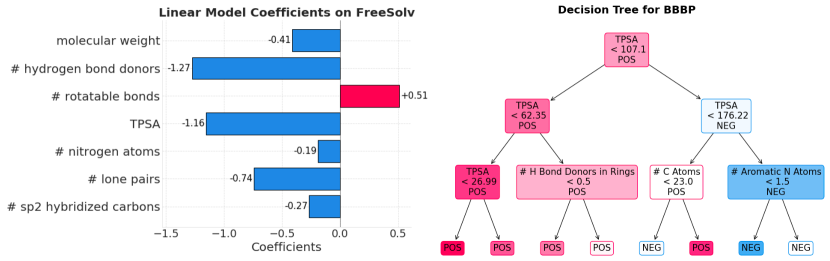
Figure 6: RQ5: Coefficients of the linear regression model and the decision tree on FreeSolv. Both with concepts refined by AutoMolCo after three iterations

Splits Interpretation of Decision Trees Complementing to the coefficients of the linear model, decision tree enhances the understanding of model’s decision process. In Figure 6 (b), we show the 3-layer decision tree for BBBP dataset. In the first two layers, the model uses TPSA to categorize the molecules into four categories, where molecules with TPSA less than 26.99 are likely to penetrate the BBB while molecules with TPSA greater than 176.22 are rarely penetrative. The decision tree further differentiates molecules with TPSA between 26.99 and 107.1 by whether or not it contains a hydrogen bond in its ring structure, where molecules without this property are more likely to penetrate the BBB. On the other hand, the model splits molecules with TPSA between 107.1 and 176.22 using the number of carbon atoms, illustrating that molecules containing more than 23 carbon atoms are very likely to be penetrative. Figure 13 shows the impurity details of the decision tree.

Concept Label Intervention Besides analyzing interpretable prediction models like linear models and decision trees, we also conduct a case study of concept label interventions with MLPs. Our goal is to identify molecules with similar concept labels except for the one we intend to intervene on (e.g., similar molecular weights, # aromatic rings, etc., except logP) but different task labels (e.g., soluble vs. insoluble). Two examples we identify from the ESOL dataset are: Diphenylamine (N(c1ccccc1)c2ccccc2) and RTI 17 (CCN2c1ccccc1N(C)C(=S)c3cccnc23). After three iterations of refinement these two molecules have the same labels for three out of the four remaining concepts, except for their logP labels, which differ by 0.275 (standardized to have mean 0 and standard deviation 1). Diphenylamine is predicted to be insoluble (-3.648), whereas RTI 17 is predicted to be soluble (-4.079), based on a conventional solubility threshold of -4 [32]. These predictions proved to be quite accurate, with the ground truth solubility of these two molecules being -3.857 and -4.227, respectively. By intervening on diphenylamine’s logP value (0.209) to match RTI 17’s logP value (0.484) through interpolation, we observe a linear change in solubility. This study highlights the significant impact of logP on solubility predictions, which is consistent with expert conclusions [22, 5], providing insights beyond traditional black-box models. We show the intervention plot in 11 in Appendix D.

4.8 Ablation studies and limitations

We conduct ablation studies of AutoMolCo. We found that AutoMolCo can perform consistently with different LLMs and is robust to molecule input formats. Also, properly combining the labeling strategies can enhance model performance. These results are in Appendix E.

Our framework also has limitations that can inspire future work. One limitation is that LLMs can sometimes hallucinate, generating inaccurate concepts and labels. This affects the accuracy and reliability of the outputs. Using more powerful LLMs could improve this issue. Another limitation is that the evaluation of the generated concepts and labels often requires validation by human experts, introducing subjectivity and dependency on domain knowledge. Developing automated evaluation methods is another potential direction for improvement.

5 Conclusion

We propose the AutoMolCo framework that automates the generation and labeling of molecular concepts, overcoming challenges of existing CMs and enhancing explainability through iterative refinement of useful concepts. We demonstrate that, for molecular property prediction tasks, simple linear prediction model on our generated concepts can perform competitively or even better than GNNs and LLM ICL. Our work paves the way for future research to further exploit the capabilities of LLMs for XAI in molecular science and beyond.

Appendices

Appendix A Example prompts

We show an example prompt for generating the labeling functions in Python code in Figure 7 and an example prompt for generating code snippet to call external tools in Figure 8.

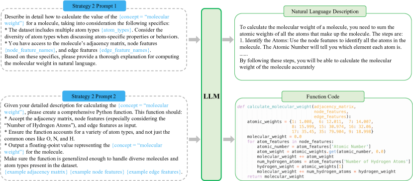
Figure 7: Prompts for generating concept labeling functions in Python code for the FreeSolv dataset.

Figure 8: Prompts for calling the external tool RDKit to label concepts on the FreeSolv dataset.

Appendix B RQ1 supplement: the full version of concept refinement

In Figure 9, we show the full list of concepts selected by AutoMolCoon FreeSolv in three refinement iterations. The result corresponds to the RQ1.

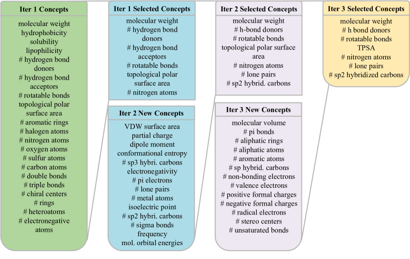
Figure 9: Concepts selected by AutoMolCo in three refinement iterations on FreeSolv. Full version.

Appendix C RQ2 supplement: challenges and solutions for concept labeling

Direct LLM prompting

For labeling with direct LLM prompting, we encountered two key issues: missing labels and unit inconsistency.

Missing labels One issue we found for concept labeling with direct LLM prompting is that it is challenging to have LLMs generate some concept labels for certain molecules. For instance, LLMs identified acid dissociation constant (pKa) as a crucial concept for predicting water solubility. However, pKa is a quantity only apply to acids, and thus the model will output “Unknown” for the label. For the ESOL dataset, this results in a $13.03\%$ missing rate for this concept. The missing-label issue underscores AutoMolCo’s limitation in recognizing concept applicability across molecules. To mitigate this, we apply various imputation methods, including mean value imputation and domain-knowledge-driven imputation. For the latter, we set missing pKa labels to $100$—significantly above water’s pKa of $14$—to denote weak or non-acidity, which enhances the CM’s performance.

Unit inconsistency We observe that for concepts with multiple possible units, labels generated by LLMs for these concepts may exhibit inconsistent units across different molecules. Take our experiments on the ESOL dataset as an example. The LLM suggest melting point as the relevant concept for predicting water solubility. When we call LLM API to generate values for melting point, it randomly chooses from Celsius (${}^{\circ}C$), Fahrenheit (F), or Kelvin (K) as melting point’s unit, which resulted in inconsistent scales for melting point’s labels. Similar issues also show up in other concepts, e.g. molecular Volume and molecular surface area. The inconsistency is due to the randomness in LLM context generation as we plug in different data instances into the prompt template. We first tried to fix the problem by specifying with LLM what unit should be used for each concept in the prompt, it was not every effective. Therefore, we added an intermediate step between Step 1 and Step 2, which lets LLM generate a concept-to-unit dictionary for each concept it proposed in Step 1. Then, we merged the resulting dictionary into Step 2’s prompt, so LLM can generate labels with consistent units based on the unit specified in the dictionary.

Function code generation

When generating labeling functions in Python code, we find it is non-trivial to prompt LLMs for executable functions with no errors. We made two efforts to increase the likelihood of producing executable functions with LLMs. We first perform prompt engineering to clearly specify atom types, adjacency matrices, and node and edge features, which enhances the function quality. Through careful prompt engineering, most generated functions for simpler concepts become executable. However, functions for labeling complex concepts like “number of rings” are still unlikely to be error-free due to their intricate nature. We thus adopt a chain of thought (CoT) approach to generate functions. For the CoT prompt, we first ask the LLM to describe the function in natural language, which can best leverage the LLM’s strength in generating natural language. Then, the CoT prompt asks the LLM to turn the natural language description of the function into Python code, which we found increases the likelihood of generating accurate and executable functions. An example of the CoT function-generation prompt is shown in Figure 7.

External tool calling

Given there are external tools for molecular science with API access, we prompt LLMs to generate code snippets for calling the tool API. We observe that LLMs are adept at obtaining callable APIs for a majority of our generated concepts from step 1, which we successfully employed to calculate the concept labels for each molecule in our dataset. The example prompts and generated API calls can be found in Figure 8. The drawback of this strategy is that the external tool cannot cover all the concepts generated by the LLM, especially for those measured concepts like melting point. For these cases, we turn to the first two strategies for labeling.

Appendix D RQ5 supplement: BBBP linear model coefficients and ESOL intervention visualization

Coefficient Interpretation of Linear Models Additional to the results in Section 4.7, we evaluating the linear model on the BBBP dataset. We focused on the top positive coefficient lipophilicity (logP) and the top negative coefficient hydrogen bond acceptors shown in Figure 10. Notably, logP has a coefficient of 1.97 and hydrogen bond acceptors has a coefficient -4.36. These finding aligns with domain knowledge, as higher logP enhances a molecule’s ability to cross lipid-rich biological membranes. Conversely, a lower number of hydrogen bond acceptors generally enhances a molecule’s permeability through the BBB. These findings validate the CM’s alignment with established biochemical principles, demonstrating its potential utility in predictive modeling for molecular properties.

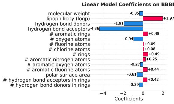
Figure 10: RQ5: Coefficients of the logistic regression model on BBBP with concepts refined by AutoMolCo after three iterations

Concept Label Intervention Complementing to the intervention study in Section 4.7, we plot the results in Figure 11.

Figure 11: Intervention on logP of diphenylamine for predicting solubility with MLP

Appendix E Ablation Studies

E.1 Different LLMs

We study the performance of AutoMolCo with different LLMs. Table 4 compares the performance of GPT-3.5 Turbo and Claude-2 using the direct LLM prompting labeling strategy with linear prediction models. While both GPT-3.5 Turbo and Claude-2 exhibit slightly inferior performance compared to GNNs across four datasets, they maintain competitive results, emphasizing simplicity and interpretability. Specifically, Claude-2 underperforms GPT-3.5 Turbo after first iteration, potentially due to its less consistent and accurate response. This inconsistency, partly attributed to more frequent issues with missing values and unit inconsistencies observed in Claude-2, suggests GPT-3.5 Turbo’s superior ability to generate reliable ground truth knowledge. Additionally, GPT-3.5 Turbo’s better prompt comprehension and domain knowledge in chemistry might contribute to its enhanced performance in predicting target concepts.

Table 4: Ablation on LLMs (GPT vs. Claude-2).

LLM	FreeSolv($\downarrow$)	ESOL ($\downarrow$)	BBBP ($\uparrow$)	BACE ($\uparrow$)
GPT-3.5	2.685	1.250	52.84	56.89
Claude-2	2.804	1.327	52.78	56.11

E.2 Direct LLM prompting with molecule names vs. with SMILES strings

Building on insights from  [13] regarding LLMs’ challenges with long molecular representations, we examined LLM’s capability in labeling concepts using SMILES strings and molecule names across our datasets. Our findings indicate that LLMs perform reasonably well in identifying basic concepts like molecular weight and atom counts using either molecule names or SMILES strings, with a strong correlation to ground truth labels ($r>0.9$). However, LLMs struggle with complex concepts requiring detailed structural knowledge, such as the number of chiral centers. Moreover, our analysis reveals a notable decline in LLM’s performance with molecule names in the larger datasets like BBBP, suggesting LLM’s familiarity with common molecular names improves its performance on smaller datasets, but this advantage diminishes with less familiar names in larger datasets. In contrast, the structural specificity of SMILES strings maintains more consistent performance across dataset sizes, highlighting their utility in representing unique molecular concepts. Furthermore, we compared the performance difference between the two representations over 3 iterations. As demonstrated in Table 5, the model performance using SMILES strings matched the model performance using molecule names on most datasets, but a notable improvement in performance with SMILES strings is observed on the BBBP dataset.

Table 5: Ablation on input formats (SMILES vs. molecule names).

	FreeSolv ($\downarrow$)		ESOL ($\downarrow$)		BBBP ($\uparrow$)		BACE ($\uparrow$)
Input Format	SMILES	Names	SMILES	Names	SMILES	Names	SMILES
GPT-3.5 iter 1	2.854	2.685	1.401	1.250	53.88	52.84	56.89
GPT-3.5 iter 2	2.662	2.520	1.262	1.250	56.08	54.05	57.60
GPT-3.5 iter 3	2.763	2.520	1.262	1.255	60.41	56.08	58.38

We also present a comparative analysis of the quality of concept labels generated using molecular names vs. SMILES strings. The comparison is visualized through a series of heatmaps, as illustrated in Figure 12.

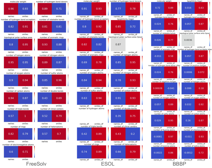
Figure 12: Correlation ($r$) between the ground truth labels and concept labels generated using molecule names or SMILES strings. Red indicates a higher correlation.

E.3 Combine different labeling strategies

The AutoMolCo framework includes three labeling strategies and allows easy extension to new ones. We consider combinations of the labeling strategies and study their impact on model performance, where we adopt a simple priority heuristic where strategy 3 $>$ strategy 2 = strategy 1. Specifically, whenever the external tool is available for a suggested concept, we get the accurate concept labels from calling it. Otherwise, two concept labels are derived from both direct prompting and function code generation, and they are both considered in step 3 for the selection. This combined-strategy labeling turns out to outperform most of the standalone strategies as shown in Table 6. These findings demonstrate that the three labeling strategies have their own strengths and weaknesses for different concepts, and they can be complement to each other to maximize the model performance. We leave exploration of new strategies and more sophisticated strategy combinations as future work.

Table 6: Combine labeling strategies.

Labeling Strategy	Model	FreeSolv($\downarrow$)	ESOL ($\downarrow$)	BBBP ($\uparrow$)	BACE ($\uparrow$)
Direct Prompt	Linear/Logistic	2.685	1.250	52.836	56.894
Direct Prompt	Tree Model	2.791	1.272	56.887	68.632
Direct Prompt	MLP	2.338	1.194	51.794	60.059
Direct Prompt + Function	Linear/Logistic	2.697	1.254	56.134	56.712
Direct Prompt + Function	Tree Model	2.540	1.364	55.150	59.998
Direct Prompt + Function	MLP	2.211	0.971	57.697	65.797
Direct Prompt + Function + Tool	Linear/Logistic	3.002	1.136	55.845	64.032
Direct Prompt + Function + Tool	Tree Model	3.752	1.107	56.250	65.658
Direct Prompt + Function + Tool	MLP	2.122	0.791	58.391	62.624

Appendix F Accuracy comparison with LLM ICL on BBBP and BACE

In our experiments, we follow the standard and widely-used evaluation metrics for all datasets. For classification tasks on BBBP and BACE, we mainly evaluate these datasets using the AUC-ROC metric and report results in our main Table 1. Since [13] provides the ICL prompts but evaluates BBBP and BACE with accuracy, we also report a comparison in accuracy in Table 7 for a fair comparison.

Table 7: Performance comparison of the AutoMolCo-induced CM vs. LLM ICL (results are taken from [13]). Results are evaluated with Accuracy ($\uparrow$).

	BBBP ($\uparrow$)	BACE ($\uparrow$)
GPT-4 (zero-shot)	0.476	0.499
GPT-4 (Scaffold, k= 8)	0.614	0.679
GPT-3.5 (Scaffold, k= 8)	0.463	0.496
Ours	0.657	0.704

Appendix G Decision trees visualization

As discussed in 4.7, we visualize the decision tree which makes the prediction process explainable. Figure 13 shows the impurity details of the decision tree shown in Figure 6 (b) and Figure 14 shows a sample decision tree for the BACE dataset.

Figure 13: The decision trees for classification on BBBP.

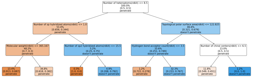
Figure 14: The decision trees for classification on BACE.

Appendix H More results on Buchwald-Hartwig and Suzuki-Miyaura

The GPT ICL performance from [13] are measured on 100 data samples. To compare AutoMolCo’s performance with their numbers, for each dataset we picked the best model performance from the logistic regression models or MLP models trained on either 200 or 500 sampled training data. The performance details are presented in Table 8 with best performance reported in Table 1.

Table 8: Performance comparison of the best AutoMolCo-induced CM vs. LLM ICL in accuracy ($\uparrow$) (GPT results are taken from [13]).

	BH ($\uparrow$)	SM ($\uparrow$)
GPT-4 (random, k = 8)	0.800	0.764
GPT-3.5 + logistic (200 samples)	0.800	0.770
GPT-3.5 + MLP (200 samples)	0.800	0.780
GPT-3.5 + logistic (500 samples)	0.790	0.780
GPT-3.5 + MLP (500 samples)	0.810	0.800

References

- Ahneman et al. [2018] DT Ahneman, JG Estrada, S Lin, SD Dreher, and AG Doyle. Predicting reaction performance in c–n cross-coupling using machine learning. Science, 2018.
- Akaike [1973] Hirotugu Akaike. Information theory and an extension of the maximum likelihood principle. In 2nd International Symposium on Information Theory, pages 267–281. Akademiai Kiado, 1973.
- Akaike [1974] Hirotugu Akaike. A new look at the statistical model identification. IEEE Transactions on Automatic Control, 19(6):716–723, 1974.
- AlKhamissi et al. [2022] Badr AlKhamissi, Millicent Li, Asli Celikyilmaz, Mona Diab, and Marjan Ghazvininejad. A review on language models as knowledge bases. arXiv preprint arXiv:2204.06031, 2022.
- Avdeef [2012] Alex Avdeef. Absorption and drug development: solubility, permeability, and charge state. John Wiley & Sons, 2012.
- Brandes et al. [2013] Ulrik Brandes, Markus Eiglsperger, Jürgen Lerner, and Christian Pich. Graph markup language (graphml), 2013.
- Bucher et al. [2019] Maxime Bucher, Stéphane Herbin, and Frédéric Jurie. Semantic bottleneck for computer vision tasks. In Computer Vision–ACCV 2018: 14th Asian Conference on Computer Vision, Perth, Australia, December 2–6, 2018, Revised Selected Papers, Part II 14, pages 695–712. Springer, 2019.
- Chen et al. [2020] Zhi Chen, Yijie Bei, and Cynthia Rudin. Concept whitening for interpretable image recognition. Nature Machine Intelligence, 2(12):772–782, 2020.
- Chung and Park [2015] Kee-Choo Chung and Hwangseo Park. Accuracy enhancement in the estimation of molecular hydration free energies by implementing the intramolecular hydrogen bond effects. Journal of Cheminformatics, 7:1–12, 2015.
- De Fauw et al. [2018] Jeffrey De Fauw, Joseph R Ledsam, Bernardino Romera-Paredes, Stanislav Nikolov, Nenad Tomasev, Sam Blackwell, Harry Askham, Xavier Glorot, Brendan O’Donoghue, Daniel Visentin, et al. Clinically applicable deep learning for diagnosis and referral in retinal disease. Nature medicine, 24(9):1342–1350, 2018.
- Guimarães and Cardozo [2008] Cristiano RW Guimarães and Mario Cardozo. Mm-gb/sa rescoring of docking poses in structure-based lead optimization. Journal of chemical information and modeling, 48(5):958–970, 2008.
- Guo et al. [2023a] Jiayan Guo, Lun Du, and Hengyu Liu. Gpt4graph: Can large language models understand graph structured data? an empirical evaluation and benchmarking. arXiv preprint arXiv:2305.15066, 2023a.
- Guo et al. [2023b] Taicheng Guo, Kehan Guo, Bozhao Nan, Zhenwen Liang, Zhichun Guo, Nitesh V Chawla, Olaf Wiest, and Xiangliang Zhang. What can large language models do in chemistry? a comprehensive benchmark on eight tasks. arXiv preprint arXiv:2305.18365, 2023b.
- Guyon et al. [2002a] Isabelle Guyon, Jason Weston, Stephen Barnhill, and Vladimir Vapnik. Gene selection for cancer classification using support vector machines. Machine Learning, 46:389–422, 2002a. doi: 10.1023/A:1012487302797.
- Guyon et al. [2002b] Isabelle Guyon, Jason Weston, Stephen Barnhill, and Vladimir Vapnik. Gene selection for cancer classification using support vector machines. Machine learning, 46:389–422, 2002b.
- Himsolt [1997] Michael Himsolt. Gml: Graph modelling language. University of Passau, 1997.
- Hu et al. [2020] Weihua Hu, Matthias Fey, Marinka Zitnik, Yuxiao Dong, Hongyu Ren, Bowen Liu, Michele Catasta, and Jure Leskovec. Open graph benchmark: Datasets for machine learning on graphs. Advances in neural information processing systems, 33:22118–22133, 2020.
- Jin et al. [2023] Bowen Jin, Gang Liu, Chi Han, Meng Jiang, Heng Ji, and Jiawei Han. Large language models on graphs: A comprehensive survey. arXiv preprint arXiv:2312.02783, 2023.
- Koh et al. [2020] Pang Wei Koh, Thao Nguyen, Yew Siang Tang, Stephen Mussmann, Emma Pierson, Been Kim, and Percy Liang. Concept bottleneck models. In International conference on machine learning, pages 5338–5348. PMLR, 2020.
- Lampert et al. [2009] Christoph H Lampert, Hannes Nickisch, and Stefan Harmeling. Learning to detect unseen object classes by between-class attribute transfer. In 2009 IEEE conference on computer vision and pattern recognition, pages 951–958. IEEE, 2009.
- Landrum [2010] Greg Landrum. RDKit: Open-source cheminformatics. https://www.rdkit.org, 2010. Accessed: Nov 22, 2023.
- Lipinski et al. [1997] Christopher A Lipinski, Franco Lombardo, Beryl W Dominy, and Paul J Feeney. Experimental and computational approaches to estimate solubility and permeability in drug discovery and development settings. Advanced drug delivery reviews, 23(1-3):3–25, 1997.
- Losch et al. [2019] Max Losch, Mario Fritz, and Bernt Schiele. Interpretability beyond classification output: Semantic bottleneck networks. arXiv preprint arXiv:1907.10882, 2019.
- Magister et al. [2021] Lucie Charlotte Magister, Dmitry Kazhdan, Vikash Singh, and Pietro Liò. Gcexplainer: Human-in-the-loop concept-based explanations for graph neural networks. arXiv preprint arXiv:2107.11889, 2021.
- Magister et al. [2022] Lucie Charlotte Magister, Pietro Barbiero, Dmitry Kazhdan, Federico Siciliano, Gabriele Ciravegna, Fabrizio Silvestri, Mateja Jamnik, and Pietro Lio. Encoding concepts in graph neural networks. arXiv preprint arXiv:2207.13586, 2022.
- Milo et al. [2002] Ron Milo, Shai Shen-Orr, Shalev Itzkovitz, Nadav Kashtan, Dmitri Chklovskii, and Uri Alon. Network motifs: simple building blocks of complex networks. Science, 298(5594):824–827, 2002.
- Oikarinen et al. [2023] Tuomas Oikarinen, Subhro Das, Lam Nguyen, and Lily Weng. Label-free concept bottleneck models. In International Conference on Learning Representations, 2023.
- Pajouhesh and Lenz [2005] H. Pajouhesh and G.R. Lenz. Medicinal chemical properties of successful central nervous system drugs. NeuroRx, 2(4):541–553, 2005. doi: 10.1602/neurorx.2.4.541. URL https://www.ncbi.nlm.nih.gov/pmc/articles/PMC1201314/.
- Pedregosa et al. [2011] F. Pedregosa, G. Varoquaux, A. Gramfort, V. Michel, B. Thirion, O. Grisel, M. Blondel, P. Prettenhofer, R. Weiss, V. Dubourg, J. Vanderplas, A. Passos, D. Cournapeau, M. Brucher, M. Perrot, and E. Duchesnay. Scikit-learn: Machine learning in Python. Journal of Machine Learning Research, 12:2825–2830, 2011.
- Petroni et al. [2019] Fabio Petroni, Tim Rocktäschel, Patrick Lewis, Anton Bakhtin, Yuxiang Wu, Alexander H Miller, and Sebastian Riedel. Language models as knowledge bases? arXiv preprint arXiv:1909.01066, 2019.
- Reizman et al. [2016] Brandon J. Reizman, Yi-Ming Wang, Stephen L. Buchwald, and Klavs F. Jensen. Suzuki–miyaura cross-coupling optimization enabled by automated feedback. React. Chem. Eng., 1:658–666, 2016. doi: 10.1039/C6RE00153J.
- Sorkun et al. [2019] Murat Cihan Sorkun, Abhishek Khetan, and Süleyman Er. Aqsoldb, a curated reference set of aqueous solubility and 2d descriptors for a diverse set of compounds. Scientific data, 6(1):143, 2019.
- Stokes et al. [2020] Jonathan M Stokes, Kevin Yang, Kyle Swanson, Wengong Jin, Andres Cubillos-Ruiz, Nina M Donghia, Craig R MacNair, Shawn French, Lindsey A Carfrae, Zohar Bloom-Ackermann, et al. A deep learning approach to antibiotic discovery. Cell, 180(4):688–702, 2020.
- Wernicke [2006] Sebastian Wernicke. Efficient detection of network motifs. IEEE/ACM transactions on computational biology and bioinformatics, 3(4):347–359, 2006.
- Wu et al. [2023] Zhengxuan Wu, Karel D’Oosterlinck, Atticus Geiger, Amir Zur, and Christopher Potts. Causal proxy models for concept-based model explanations. In International conference on machine learning, pages 37313–37334. PMLR, 2023.
- Wu et al. [2018] Zhenqin Wu, Bharath Ramsundar, Evan N Feinberg, Joseph Gomes, Caleb Geniesse, Aneesh S Pappu, Karl Leswing, and Vijay Pande. Moleculenet: a benchmark for molecular machine learning. Chemical science, 9(2):513–530, 2018.
- Xuanyuan et al. [2023] Han Xuanyuan, Pietro Barbiero, Dobrik Georgiev, Lucie Charlotte Magister, and Pietro Liò. Global concept-based interpretability for graph neural networks via neuron analysis. In Proceedings of the AAAI Conference on Artificial Intelligence, volume 37, pages 10675–10683, 2023.
- Yeh et al. [2020] Chih-Kuan Yeh, Been Kim, Sercan Arik, Chun-Liang Li, Tomas Pfister, and Pradeep Ravikumar. On completeness-aware concept-based explanations in deep neural networks. Advances in neural information processing systems, 33:20554–20565, 2020.
- Yi et al. [2018] Kexin Yi, Jiajun Wu, Chuang Gan, Antonio Torralba, Pushmeet Kohli, and Josh Tenenbaum. Neural-symbolic vqa: Disentangling reasoning from vision and language understanding. Advances in neural information processing systems, 31, 2018.
- Yu et al. [2024] Botao Yu, Frazier N. Baker, Ziqi Chen, Xia Ning, and Huan Sun. Llasmol: Advancing large language models for chemistry with a large-scale, comprehensive, high-quality instruction tuning dataset, 2024.
- Yu and Gao [2022] Zhaoning Yu and Hongyang Gao. Molecular representation learning via heterogeneous motif graph neural networks. In International Conference on Machine Learning, pages 25581–25594. PMLR, 2022.
- Yuan et al. [2022] Hao Yuan, Haiyang Yu, Shurui Gui, and Shuiwang Ji. Explainability in graph neural networks: A taxonomic survey. IEEE transactions on pattern analysis and machine intelligence, 45(5):5782–5799, 2022.
- Zhang [2023] Jiawei Zhang. Graph-toolformer: To empower llms with graph reasoning ability via prompt augmented by chatgpt. arXiv preprint arXiv:2304.11116, 2023.
- Zhang et al. [2020] Shichang Zhang, Ziniu Hu, Arjun Subramonian, and Yizhou Sun. Motif-driven contrastive learning of graph representations. arXiv preprint arXiv:2012.12533, 2020.
- Zhang et al. [2023] Xuan Zhang, Limei Wang, Jacob Helwig, Youzhi Luo, Cong Fu, Yaochen Xie, Meng Liu, Yuchao Lin, Zhao Xu, Keqiang Yan, et al. Artificial intelligence for science in quantum, atomistic, and continuum systems. arXiv preprint arXiv:2307.08423, 2023.